introductionto r · i set the working directory to the folder "tp0" either using the pane...

Université Paris DauphineDépartement MIDOLicence 3 – Statistical Inference (1): estimation

2017–2018

Introduction to R

Jean-Michel MARIN, Robin RYDER and Julien STOEHR

Contents

1 Introduction 2

2 How to use R? 2

2.1 Using a command-line user interface . . . . . . . . . . . . . . . . . . . . . . . . . . . . . 2

2.2 Using RStudio . . . . . . . . . . . . . . . . . . . . . . . . . . . . . . . . . . . . . . . . . . . 3

2.3 Getting help . . . . . . . . . . . . . . . . . . . . . . . . . . . . . . . . . . . . . . . . . . . . 4

2.4 Working directory . . . . . . . . . . . . . . . . . . . . . . . . . . . . . . . . . . . . . . . . . 5

2.5 Libraries . . . . . . . . . . . . . . . . . . . . . . . . . . . . . . . . . . . . . . . . . . . . . . 5

3 R Objects 6

3.1 Vectors . . . . . . . . . . . . . . . . . . . . . . . . . . . . . . . . . . . . . . . . . . . . . . . 8

3.2 Matrices . . . . . . . . . . . . . . . . . . . . . . . . . . . . . . . . . . . . . . . . . . . . . . 10

3.3 Arrays . . . . . . . . . . . . . . . . . . . . . . . . . . . . . . . . . . . . . . . . . . . . . . . . 11

3.4 Lists . . . . . . . . . . . . . . . . . . . . . . . . . . . . . . . . . . . . . . . . . . . . . . . . . 12

3.5 Data Frames . . . . . . . . . . . . . . . . . . . . . . . . . . . . . . . . . . . . . . . . . . . . 13

4 Usual distributions 14

5 Some useful functions for exploratory statistics 15

6 Plots in R 16

6.1 Histograms . . . . . . . . . . . . . . . . . . . . . . . . . . . . . . . . . . . . . . . . . . . . . 17

6.2 Scatter plots . . . . . . . . . . . . . . . . . . . . . . . . . . . . . . . . . . . . . . . . . . . . 17

6.3 Options common to histograms and scatter plots . . . . . . . . . . . . . . . . . . . . . . 18

6.4 Additions to an existing plot . . . . . . . . . . . . . . . . . . . . . . . . . . . . . . . . . . . 18

6.5 Example . . . . . . . . . . . . . . . . . . . . . . . . . . . . . . . . . . . . . . . . . . . . . . 19

7 Building a new function 20

8 Few notions of programming: conditional constructs and loops 21

9 Handling created objects 23

1

J.-M. Marin, R. Ryder, J. Stoehr Introduction to R

1 Introduction

R is an interpreted programming language, and a free software environment particularly useful for

statistical computing and graphics. Created in the early 1990s by Robert Gentleman and Ross Ihaka,

it is a free clone of S-Plus (software sold by MathSoft based on the S programming language).

R is currently developed by the R Core Development Team. It provides through libraries a wide range

of statistical methods an graphical facilities. All the useful information on R can be found on the

R Core Development Team website https://www.r-project.org. In particular, the latest versions

of R distributions and documentation can be downloaded from the website.

R is also substantially extended by user-created packages, a flexible manner for users to add some

functionnalities. Amongst other options, packages are available on The Comprehensive R archive

network (CRAN, https://cran.r-project.org/).

The present document is solely a short introduction on the tools we will use throughout the course.

For a more comprehensive overview on the use of R , we suggest to read the manual R for be-

ginners by Emmanuel Paradis and available at https://cran.r-project.org/doc/contrib/Paradis-rdebuts_en.pdf.

2 How to use R?

2.1 Using a command-line user interface

On Unix systems, R is accessible from a console user interface and does not require a graphical user

interface. Once the software installed, it can be run by entering the command R in a Terminal.

When R is opened, the Terminal line starts with the character >. This signals that the console is

available for you to type an instruction. When you type an unfinished instruction (for example if

you open a parenthesis and do not close it before pressing Enter), the console line starts with the

character + instead, indicating that R is waiting for the end of the instruction.

Exercice 1. Starting with R and the command line interface

I Open a Terminal.

I Start the software R by typing R and then press Enter. The Software is now waiting for your

command lines.

I Type the simple operation 3 + 5, then press enter.

I To quit the R session, type q(), press enter and answer n.

I Close the Terminal.

The main drawback on using a command-line interface is that commands are executed on the go.

For advanced programming, an alternative is to edit a script, for example script.R , in a text editor

2

https://www.r-project.org

https://cran.r-project.org/

https://cran.r-project.org/doc/contrib/Paradis-rdebuts_en.pdf

https://cran.r-project.org/doc/contrib/Paradis-rdebuts_en.pdf


and then to call it using the command source("script.R"). By default the command sourcesimply reads and executes the R code from a file but does not prompt the command line or the

output. In order to print the command line before its evaluation, the command source has an

option echo taking logical values TRUE or FALSE, and in order to print the result of evaluation,

it has an option print.eval taking logical values TRUE or FALSE. You can read more on the the

command source at https://www.rdocumentation.org/packages/base/versions/3.4.1/topics/source.

2.2 Using RStudio

In what follows, we use the integrated development environment (IDE) RStudio (https://www.rstudio.com) which offers an easy-to-use Graphical User Interface available for all the plateform

(iOS, Linux and Windows). But other IDE could have been used such as RKward, R Commander or

R Tools for Visual Studio (plug-in for Microsoft Visual Studio) to name just a few.

In most IDEs, you will find information stored in several windows which offer a more flexible and

efficient manner to use R rather than the simple command line interface. The most important ones

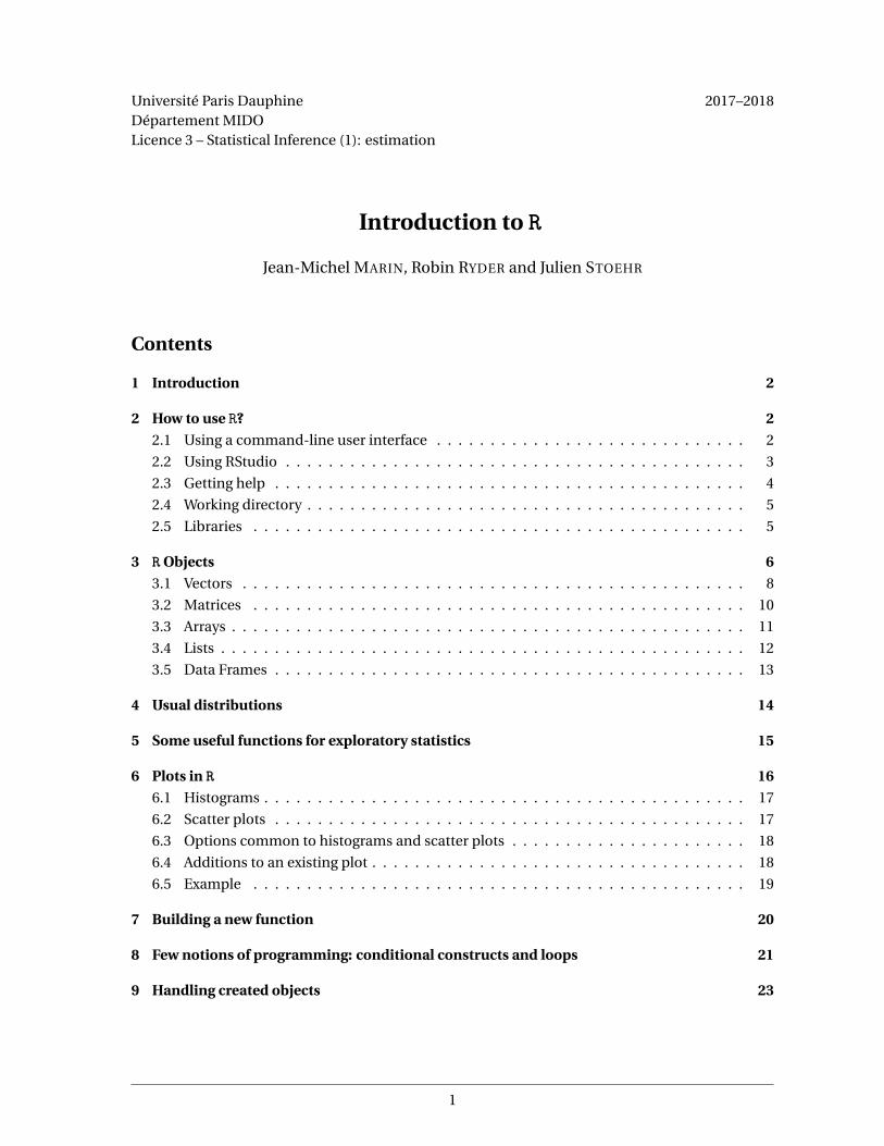
are the Console window and the Script or Editor window. Hereafter is the organisation of RStudio

interface, see Figure 1.

The Console window (1): by default, it is the bottom left window. It allows to enter command lines

after the prompt ">" in the same way as in the Terminal.

(1) Code Editor window:your script will appear here

(2) R console: your com-mand lines are excuted here

(3) Environment and History

(4) File system, Plots,Packages and Help

Figure 1: RStudio. Organisation of the different windows by default.

3

https://www.rdocumentation.org/packages/base/versions/3.4.1/topics/source

https://www.rdocumentation.org/packages/base/versions/3.4.1/topics/source

https://www.rstudio.com

https://www.rstudio.com


The Script or Editor window (2): by default, it is the top left window. Each pane corresponds to a file

with extension .R (called script) made of R command lines (and eventually comments indicated by

a line starting with symbol #). A script is particularly useful because it allows to save the command

lines in a file but also allows to implement more complex codes. To run the code in the Console

window, the user can:

(i) use the button "Run". The current line or the selected lines will be sent to the Console.

(ii) press "ctrl+enter". The current line or the selected lines will be sent to the Console.

(iii) use the button "Source". The whole code is sent to the Console. If you wish to print the

command line and their evaluations, use the button "Source with Echo" instead.

When working on a script, you should very regularly save your file with extension .R.

The Workspace or Environment window (3): by default, the top right window contains 2 or 3 panes.

The first one called "Environment" lists all the data and objects stored in the current R session

memory. The second one called "History" shows the historic of all the command lines you typed or

loaded into the Console. You can save your console history as a file with extension .Rhistory. The

last one called "Viewer" allows to view local web content.

Files, Plots, Packages, Help (4): by default, the bottom right window contains 4 panes. The pane

"Files" corresponds to the file system. The various graphics produced by R are displayed in the pane

"Plots". A list of installed packages (you can pick the one you want to load or not) is available in the

pane "Packages". Finally, the pane "Help" contains the help documentation.

Exercice 2. Starting with RStudio

I Open RStudio

I Type the simple operation 3 + 5 in the Console, then press enter.

I Create a script: from the toolbar go to "File > New File > R Script" (an untitled file appears

in the Editor window).

I Type the operation 3 + 5 in the Editor window and execute it.

I Quit RStudio either using "File > Quit Session" from the toolbar or by typing q() in the Con-

sole.

2.3 Getting help

If internet provides a wide help documentation (the website https://www.rdocumentation.orgis a perfect example), you can get the documentation on any function or object JohnDoe and its

uses from the command line interface by using the command help(JohnDoe) or its highly helpful

shortcut ?JohnDoe. In RStudio, you can also get help from the pane Help (by default in the bottom

right window, see Figure 1). It is also possible to get help in HTML format using the command

help.start().

4

https://www.rdocumentation.org


Exercice 3. Getting help on Source

1. In a Terminal:

I try help(source) and ?source. To quit the documentation press q.

2. In RStudio:

I try help(source) and ?source in the Console and Editor windows.

I search for the documentation in the "Help" pane.

2.4 Working directory

The working directory is the location in the file system where R writes and reads information by

default. The command getwd() provides the current working directory. In order to select another

working directory, three options are available:

(i) the command line setwd("path_to_directory" ) allows to specify the path to the working

directory;

(ii) in the pane "Files" from the bottom right window, navigate in the file system till you are at the

desired location, then click on menu "More" and select "Set As Working Directory";

(iii) in the menu "Session" from the toolbar (for some version of RStudio in the menu "Tools"

from the toolbar), go to "Set Working Directory > Choose Directory..." and select the desired

location.

2.5 Libraries

R provides numerous tools to run statistical analysis. The various functions as well as some datasets

are stored in libraries which should be loaded in order to have access to their contents. A library

can be loaded:

(i) either with the command line library(library_to_load ),

(ii) or by ticking the library in the pane "Packages" from RStudio,

and it can be unloaded:

(i) either with the command line detach(package:library_to_unload ),

(ii) or by unticking the library in the pane "Packages" from RStudio.

A huge range on libraries can be found on internet. Most of them are available on the CRAN and

can be installed using:

(i) either with the command line install.packages(library_to_install ).

5


(ii) or by clicking on the Install button in the pane "Packages" from RStudio and then by selecting

the desired package in the list.

Exercice 4. Working directory and libraries

I Create a new folder "statistics_estimation" and a subfolder "TP0".

I Download in "TP0" the file "script_example.R" from https://sites.google.com/site/statistics1estimation/.

I Fill line 8 in "script_example.R" to add the MASS library and line 32 to unload the Mass

library.

1. In a Terminal:

I start R and find the current working directory.

I Set the working directory to the folder "TP0".

I Type the command source("script_example.R"), then press enter. What is happen-

ing?

I Type the command source("script_example.R", echo = TRUE), then press enter.

What is the option "echo" doing?

I Type the command source("script_example.R", print.eval = TRUE), then press

enter. . What is the option "print.eval" doing?

I Why does the previous command source("script_example.R", echo = TRUE) print

functions evaluation?

2. In RStudio:

I find the current working directory.

I Set the working directory to the folder "TP0" either using the pane "Files" or using "Ses-

sion" from the toolbar.

I Open "script_example.R" using the pane "Files" or "File" from the toolbar and add a

command line at the top of the document to set the working directory to the folder "TP0".

I Execute the script. The histogram appears in the pane "Plots".

I Load and unload the library MASS using the pane "Packages".

3 R Objects

The basic elements of R are organised in a data structure which includes vectors, matrices, arrays,

data frames and lists. But it contains some more complex and extensible objects such as regression

models and time-series to name but a few. Note that there is no structure corresponding to scalar

in R . A scalar is represented by a single-element vector. R is not limited to the those programming

features and also allows to define functions (see Section 7).

6

https://sites.google.com/site/statistics1estimation/

https://sites.google.com/site/statistics1estimation/


A R object is defined by its class which describes data’s structure and by its type which describes the

contents. Whithout being exhaustive, the main types are:

• null (empty object),

• logical,

• integer,

• numeric,

• complex,

• character.

A logical value is encoded using the strings TRUE and False, or altenatively using their abbrevia-

tions T and F. Decimal numbers must be encoded with a decimal point while character strings must

be in between double quotes " ". Finally, missing values are encoded by the character string NA.

The following table shows some possible types for a given class:

Structure Type

VectorHomogeneous: can contain only one type among null, logical, integer, numeric,complex or character

MatrixArrayTime-serieData frame heterogeneous: can contain elements of different types among null, logical,

integer, numeric, complex or characterList

When creating an object in R , it is possible to assign it. For assignement it is possible to use either =

or <-, but we advocate in favor of the back arrow in this course for the sake of clarity and readibility.

Example 1.

> # The following line is interpreted as the sum of two vectors> # of size one and will return a vector of size one.> 3 + 5

[1] 8

> # The following line assigns the value of the sum to the> # variable a> a <- 3 + 5

Given an object x, it is possible to test for its structure/type (variable information) or to convert its

structure/type (variable conversion).

Variable information: R contains methods whose prefix is is., such as:

• is.null(x),

• is.logical(x),

• is.numeric(x),

• is.complex(x),

• is.character(x),

• is.vector(x),

• is.matrix(x),

• is.data.frame(x),

• is.list(x).

Variable conversion: R provides methods whose prefix is as, like:

• as.logical(x),

• as.numeric(x),

• as.complex(x),

• as.character(x),

• as.vector(x),

• as.matrix(x),

• as.data.frame(x),

• as.list(x).

7


3.1 Vectors

Vectors are the most basic object in R . A vector is made of an ordered collection of elements of same

nature which, as already mentionned, can be numerical, logical or alphanumerical. A vector can be

manually built using the command c(item1, item2,. . .).

Exercice 5. Type the following commands in a console.

1. Creating a vector

a <- c(3, 5.6, 1, 4, -7) Assign a numerical vector of length 5 with values 3, 5.6,

1, 4, - 7 to variable aa Display vector abool <- a == 4 Assign boolean vector of the length of a and whose val-

ues are TRUE if the corresponding component of a is

equal to 4 and FALSE otherwise

text <- c("big","small") Assign a character vector of length 2 with values bigand small to variable text

2. Accessing or extracting elements

a[1] Return the first value of vector aa[-2] Return all but the second element of vector aa[1:3] Return first 3 elements of vector aa[-(1:3)] Return elements from 4 to the end of vector aa[2:4] Return elements from 2 to 4 of vector aa[-(2:4)] Return all but elements from 2 to 4 of vector aa[1,4,2] Return an error message

a[c(1,4,2)] Return specific elements 1, 4 and 2 (in that order) of aa[a > 2] Return all elements greater than 2 in vector aa[a > 2 & a < 4] Return all elements between 2 and 4 in vector atext[text %in% c("b","medium", "small")]

Return elements of text that are in the given set {b,medium, small}

3. Useful functions for a vector

is.vector(text) Function is.vector() returns the logical value TRUE if

its argument is a vector and FALSE otherwise.

length(a) Return the number of elements of asum(a) Return the sum of all elements of at(a) Return the transpose vector. The result is a row vector

4. Operations with a scalar

2*a Product by a scalar

8


b <- a-4 Subtraction of a scalar: create a vector with the length

of a and whose values are equal to those of a minus 4,

then assign it to b

5. Operations between vectors

d <- a[c(1,3,5)]e <- 3/d Create a vector e with the same length than d and whose

elements i is equal to 3/d[i]

d+e Summation of vectors d and ed-e Difference of vectors d and ed <- d+e Replace d by the vector resulting from adding d and ed*e Element-wise multiplication of vectors d and ee/d Element-wise division of vector e by vector dt(d)%*%e Scalar product of row vector t(d) and column vector e

6. Generating replicated vectors

x <- 1:5 Create a vector x of integers between 1 and 5

rep(x, 2) Replicate vector x two times

rep(x, each = 2) Replicate each element of x two times

?rep Access the help page of function rep()

7. Generating a sequence

seq(0, 1, length = 11) Return a sequence of 11 equaly spaced elements be-

tween 0 and 1

seq(1.575, 5.125,by=0.05)

Return a sequence between 1.575 and 5.125 with in-

crement 0.05?seq Access the help page of function seq()

8. Generating random samples

sample(c(0,1), 10,replace = T)

Sampling from {0,1} 10 times with replacement

sample(c(1,2,3),3) Random permutation: sampling from {1,2,3} without

replacement

letters[2] Return the second letter (lower case) of the alphabet

LETTERS[2] Return the second letter (capital) of the alphabet

sample(letters[1:9], 5) Sample 5 letters among the first 9 without replacement

?sample Access the help page of function sample()

9. Transforming a vector

sort(a) Sort vector a into ascending (by default) or descending

order

9


order(a) Return the permutation to rearrange elements of a in

ascending (by default) or descending order

?order Access the help page of function order()abs(d) Return the absolute values of elements of dexp(d) Return the exponential values of elements of dlog(abs(d)) Return the log values of elements abs(d)

3.2 Matrices

Like vectors, matrices can be of any type, but cannot contain elements of different types. The syntax

to create a n×p matrix is: matrix(vec, nrow = n, ncol = p) where vec is a vector containing

the elements of the matrix which will be filled by column unless the option byrow = T is included.

The elements of vec are recycled, i.e., reused till the matrix is full. Note:

• if vec is a single-element vector, the matrix generated with the aforementionned command will

be filled with the value of vec;

• if vec is a non single-element vector, it is not mandatory to specify both nrow and ncol. Only

one dimension is required, for example nrow, the second dimension, for example ncol, being

the number of element in vec divided by ncol;

• if both nrow and ncol are specified and the number of elements in vec is not a multiple or a

divider of n ×p a warning message will be printed since some elements will be omitted.


1. Creating a matrix

a <- 1:20b <- sample(1:10, 20, replace = T)M <- matrix(a, nrow = 5) Create a numerical matrix M from a with 5

rows and length(a)/5 = 4 columns by fill-

ing it by columns

N <- matrix(a, nrow = 5, byrow =T)

Create a numerical matrix N from a with 5

rows and length(a)/5 = 4 columns by fill-

ing it by rows

O <- matrix(b, ncol = 10) Create a numerical matrix O from b with 10

columns and length(b)/2= 2 rows by filling

it by columns

P <- matrix(NA, 2, 5) Create a 2×5 matrix P filled with NA

M; N; O; P Display consecutively matrices M, N O and P


M[3,2] Return element on the 3rd row and 2nd column of M

10


M[5,] Return 5th row of MM[,2] Return 2nd column of MM[c(1,3,4),] Return 1st, 3rd and 4th rows of MM[,c(1,4)] Return 1st and 4th columns of MM[-2,] Remove 2nd row of MM[,-3] Remove 3rd column of MM[-c(1,3),] Remove 1st and 3rd rows of MM[,-c(2,4)] Remove 2nd and 4th columns of MO>5 Display a matrix of booleans where element [i,j] is TRUE if

a[i,j]>5O[O<5] <- 0 Set to 0 all elements of a lower than 5

diag(M) Return the diagonal, i.e., all the elements M[i,i], of Mdiag(M) <- 1 Set to 1 the diagonal, i.e., all the elements M[i,i], of M

3. Useful functions for a matrix

dim(M) Return the dimensions of matrix Mnrow(M) Return the number of rows of Mncol(M) Return the number of columns of MQ <- t(N) Transpose matrix Napply(M, 2, sum) Return the sum of M column-wise (deprecated)

colSums(M) Faster version of apply(M,2,sum)apply(M, 1, sum) Return the sum of M row-wise (deprecated)

rowSums(M) Faster version of apply(M,2,sum)

4. Operations with a scalar

3*O Product by a scalar: each component of O is multiplied by 3

Q-4 Subtraction of a scalar: substract 4 to each element of Q

5. Operations between matrices: R controls dimension adequacy!

M*N Element-wise multiplication between M and NM%*%Q Matrix product between M and QM*Q Print an error message due to incompatible dimension for

element-wise product

M%*%N Print an error message due to incompatible dimension for matrix

product

rbind(M, N) Vertical concatenation of matrices M and Ncbind(M, N) Horizontal concatenation of matrices M and N

3.3 Arrays

The object array is aimed for matrices with more than two dimensions. The data creation relies on

the command array(vec, c(n,p,q...)) where vec is a vector giving data used to fill the array

11


by column, and the argument c(n,p,q...) gives the dimensions: n is the number of rows, p the

number of columns, q the number of matrices...


1. Creating an array

x <- array(1:50,c(2,5,5))

Create an array x with 5 matrices of dimension 2× 5

from vector 1:50

x Display x


x[1, 2, 3] Return the element on the 1st row, 2nd column in the 3nd matrix

3. Useful functions for an array

dim(x) Return the dimensions of the array xaperm(x) Generalized transpose of x: x[i,j,k] becomes x[k,j,i]

3.4 Lists

A list is an ordered collection of objects which can be of different types. The elements of a list can

thus be any objects defined in R. This property is used by some functions to return complex results

as a single object.

Creating a list of named or unnamed arguments is done using the command list(name1 = item1,name2 = item2, ...) where the names are optional. Each element of a list can be accessed ei-

ther with its index or name in double square brackets: name_of_list [[index_of_argument ]]or with its name preceded by the symbol $: name_of_list $name_of_argument .


1. Creating a list

L <- list(num = 1:5,letters[1:3], bool = T)

Create a list L with 1st and 3rd arguments

named and 2nd argument unnamed

L


L$num Return the element named num in LL[["num"]] Return the element named num in LL$a Return NULL: no element named a in LL[[1]] Return the 1st element of LL[[2]] Return the 2nd element of L

12


3.5 Data Frames

In R, a data frame is similar to a matrix but the columns can be of various types. Data frames

constitute a special class of lists devoted to storing data for analysis. Each component of the list

is the equivalent of a column or variable, and the elements of these components correspond to

rows or individuals. Specific methods for statistical analysis are associated with this class.

The command data.frame(name1 = var1, name2 = var2, ...) creates a data frame of named

or unnamed variables. If the group of variables did not share the same length, shorter vectors are

recycled to the length of the longest. A data frame can also be created from an external file using

the command read.table(...).

Data frames are a structure where data conversion is quite useful. Indeed, it is possible to transform

a matrix M into a data frame with the command as.data.frame(M). The reverse transformation is

also possible with the command as.matrix but is somewhat more delicate. If the data frame is

homogenous and contains only numerical values, the command will return a numerical matrix.

Althought in the most common case of heterogeneous data, the matrix will be of character type.


1. Creating a data frame

v1 <- sample(1:12, 30, replace = T)v2 <- sample(LETTERS[1:10], 30, replace = T)v3 <- runif(10) 10 independent realisations of the uniform distri-

bution over [0,1] (see Section 4)

v4 <- rnorm(15) 15 independent realisations of the normal distri-

bution with mean 0 and variance 1 (see Section 4)

v1;v2;v3;v4df <- data.frame(v1, v2, v3,v4)

Create a data frame with 30 observations of 4 vari-

ables. Observations of v3 and v4 are replicated to

the length of v1df

2. Accessing or extracting elements: the command to access matrices elements are also avail-

able for data frames.

df$v2 Return the observations of variable named v2df[["v1"]] Return the observations of variable named v1

3. Data conversion

M <- matrix(1:15, nrow = 3)M <- as.data.frame(M) Convert M into a data frame

is.data.frame(M) Test if M is a data frame

13


N <- as.matrix(df) Convert df into a matrix (type character) and as-

sign it to N

4. Dealing with data

data() Open a window listing all data framesavailable in

R

data(women) Load data frame womennames(women) Display variable names of data frame womenheight Return an error message

attach(women) Database women attache to R: objects in the

database can be accessed by simply giving their

names

height Return women$height (because women is now at-

tached to R)

4 Usual distributions

R provides usual probability distributions listed below:

Distribution Name Parameters Default values

Beta beta shape1, shape2Binomial binom size, probCauchy cauchy location, scale location = 0, scale = 1Chi-Squared chisq dfExponential exp rate (= 1/mean) rate = 1Fisher f df1, df2Gamma gamma shape, rate (= 1/scale) rate = 1Geometric geom probHypergeometric hyper m, n, kLog-Normal lnorm mean, sd mean = 0, sd = 1Logistic logis location, scale location = 0, scale = 1Normal norm mean, sd mean = 0, sd = 1Poisson pois lambdaStudent t dfUniform unif min, max min = 0, max = 1Weibull weibull shape

For each distribution available, there are four commands prefixed by letters d, p, q and r, and

followed by the name of the distribution. For instance, dnorm, pnorm, qnorm and rnorm are the

commands corresponding to the normal distribution, and dweibull, pweibull, qweibull and

rweibull the ones corresponding to the Weibull distribution.

14


• dname denotes either the probability density function for a continuous variable or the proba-

bility mass function, i.e., P(X = k), for a discrete variable.

• pname denotes the cumulative distribution function, i.e., P(X ≤ x).

• qname denotes the quantile function, in other words the value at which the cumulative distri-

bution function reaches a certain probability. In the continuous case, if pname(x) =p then qname(p) = x. In the discrete case, it returns the smallest integer u such that

P(X ≤ u) ≥ p.

• rname generates independent random realisations from the distribution.

Exercice 10. Comment the following commands line

qnorm(0.975)pnorm(1.96)rnorm(5)dnorm(0)x <- seq(-1,1,0.25)dnorm(x)rnorm(3, 5, 0.5)dunif(x)runif(3)rt(5,10)

5 Some useful functions for exploratory statistics

The current section is the opportunity to list some of the most useful functions to sumarize data.

Function Brief description

summary Compute summaries of observed data contained in a vector (of type numeric,factor, ...) or in a data frame, column by column

For a vector of observations of a quantitative variablemean Empirical meansd Empirical standard deviationvar Empirical variance: unbiased estimator (the denominator is n −1)median Empirical medianquantile Empirical quantilescor Empirical linear correlation coefficient between two variables

For a vector of observations of a qualitative variabletable(v2) Summary of qualitative variable

15


Exercice 11. Comment the following commands line

data(women); names(women)attach(women)mean(height); var(height); sd(height); median(height); quantile(height)summary(weight)summary(women)

6 Plots in R

Plots are useful to visualize your results and a major tool to check that you have obtained what was

required. It is important to use the correct options when plotting an object as the default values can

sometimes lead to wrong plots! Hereafter are listed some of the major graphical tools you will use.


plot Generic function for plotting an abject (point clouds, curves, barplot, ...)hist Draw histogram in frequencies or probability densitiestruehist Alternative to draw histogram from the library MASSboxplot Draw one or many boxplot in parallelpie Draw a pie chart

plot and hist are described in more detail below and we refer to the R documentation for more

details on the other graphical tools.

The graphical possibilities in R are not limited to the aforementionned. For example, the libraries

ggplot2 has encountered a growing success and offers flexible tools to produce high quality plots.

However its use will not be addressed in this course. Visit the webpage http://ggplot2.org for

more details on ggplot2.

Preliminary remarks

A useful webpage to read concerning graphics is http://www.statmethods.net/graphs/creating.html

Graphical parameters. The command par is useful to set some graphical parameters. For in-

stance par(mfrow = c(nrow, ncol)) allows to display several plots side by side on nrow rows

and ncol columns. It is also possible to modify the margin of the graphical window with the com-

mand par(mai = c(..., ..., ..., ...)). Many other graphical options are available: see

?par. See for example http://www.statmethods.net/advgraphs/parameters.html.

Navigating betwenn plots. When drawing many plots on different windows, it is possible in RStu-

dio to naviagte between plots using the blue arrows from the "Plots" pane. When using a com-

mand line interface, viewing several plots at a time may sometimes be problematic since a new

16

http://ggplot2.org

http://www.statmethods.net/graphs/creating.html


http://www.statmethods.net/advgraphs/parameters.html


plot will overwrite the previous one. But solution exists as shown at http://www.statmethods.net/graphs/creating.html.

Saving a plot. In RStudio, once a plot has been drawn, it can be saved in various format using

the button "Export" from the "Plots" pane. It is also possible to save a plot as .eps or .pdf file

using the command line dev.copy2eps(file = "plotname.eps") or dev.copy2pdf(file ="plotname.pdf"): see for example ?dev.copy2eps and ?dev.copy2pdf. For some alternatives,

see http://www.statmethods.net/graphs/creating.html.

6.1 Histograms

Histograms are mostly used to visualize a distribution. The syntax to draw a histogram is hist(x,list of options), where x is the dataset. The following options are useful:

• breaks = N to specify the number N of classes (of "bars");

• freq = F to display a histogram in probability (total area of one), rather than in counts

(which is the default). Alternatively you can use the option probability = T.

Exercice 12. Observe the difference between the two following histograms

data(women); attach(women)hist(height, breaks = 15)hist(height, breaks = 15, freq = F)

6.2 Scatter plots

Scatter plots are useful to visualize the link between two variables. The syntax to draw such a plot is

plot(x, y, list of options). Note that plot(x, options) puts the variable x on the y-axis

and the indices on the x-axis.

By default, the command plots a point cloud which correspond to the option type = "p". The

properties of the points can be edited using:

• pch = ... change the symbol for points. For example pch = 19 to have solid circle or pch =15 to have filled square;

• cex = ... change the size of points.

It is possible to have lines between points too:

• type = "l" option to have lines between points;

• type = "b" option to have both points and lines.

17





Exercice 13. Draw the following scatter plots

x <- seq(0, 1, 0.1); plot(x, x - x * x + 2)plot(x, x - x * x + 2, type = "l")plot(x, x - x * x + 2, type = "b", pch = 19)

6.3 Options common to histograms and scatter plots

Hereafter some helpful options to customize a plot are listed especiallyto add titles and captions.


col = ... To change the color. For example col = "blue" (quotation marksare important). A useful guide of color is available at http://www.stat.columbia.edu/~tzheng/files/Rcolor.pdf

lty = ... To change the line type. For example lty = 1 for solid line or lty= 2 for dashed line

lwd = ... To change the line widthmain = "myTitle" To add a title displayed above the plotxlim = c(xmin, xmax) To choose the range of the x-axisylim = c(ymin, ymax) Same than xlim but for the y-axisxlab = ("x caption") To change the caption on the x-axisylab = ("y caption") Same than xlab but for the y-axiscex.main = ... To change the size of main titlecex.axis = ... To change the size of axis annotationcex.lab = ... To change the size of axis labels

6.4 Additions to an existing plot

The following functions allow to add graphical element to an existing plot. The various graphical

options are available for those functions as well.


points(x, y) Add a point cloud using the same principle as plot(x, y,type = "p")

lines(x, y) Add lines between the coordinates of x and y using the sameprinciple as plot(x, y, type = "l")

abline(v = a) Add a vertical line of equation x = aabline(h = b) Add a horizontal line of equation y = bcurve(fonction, add = T) Add a curve to an existing plot. Note that without add = T, a

new plot is created

When adding elements to an existing plot, it is recommanded to add a legend for the readibility of

the graph. This can be achieve using the function legend.

18

http://www.stat.columbia.edu/~tzheng/files/Rcolor.pdf

http://www.stat.columbia.edu/~tzheng/files/Rcolor.pdf


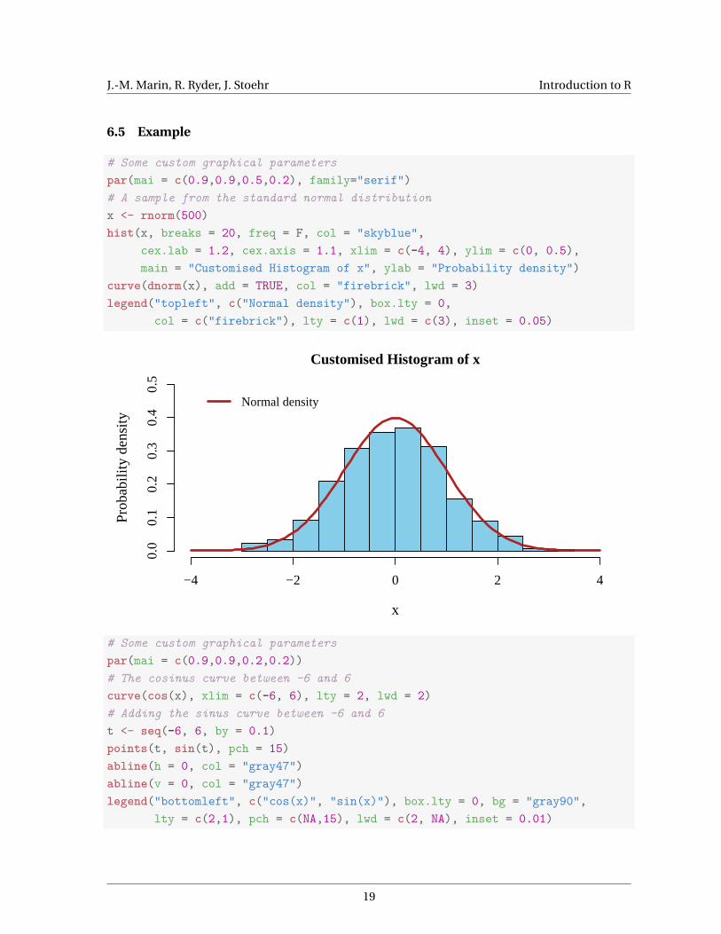
6.5 Example

# Some custom graphical parameterspar(mai = c(0.9,0.9,0.5,0.2), family="serif")# A sample from the standard normal distributionx <- rnorm(500)hist(x, breaks = 20, freq = F, col = "skyblue",

cex.lab = 1.2, cex.axis = 1.1, xlim = c(-4, 4), ylim = c(0, 0.5),main = "Customised Histogram of x", ylab = "Probability density")

curve(dnorm(x), add = TRUE, col = "firebrick", lwd = 3)legend("topleft", c("Normal density"), box.lty = 0,

col = c("firebrick"), lty = c(1), lwd = c(3), inset = 0.05)

Customised Histogram of x

x

Pro

babi

lity

dens

ity

−4 −2 0 2 4

0.0

0.1

0.2

0.3

0.4

0.5

Normal density

# Some custom graphical parameterspar(mai = c(0.9,0.9,0.2,0.2))# The cosinus curve between -6 and 6curve(cos(x), xlim = c(-6, 6), lty = 2, lwd = 2)# Adding the sinus curve between -6 and 6t <- seq(-6, 6, by = 0.1)points(t, sin(t), pch = 15)abline(h = 0, col = "gray47")abline(v = 0, col = "gray47")legend("bottomleft", c("cos(x)", "sin(x)"), box.lty = 0, bg = "gray90",

lty = c(2,1), pch = c(NA,15), lwd = c(2, NA), inset = 0.01)

19


−6 −4 −2 0 2 4 6

−1.

0−

0.5

0.0

0.5

1.0

x

cos(

x)

cos(x)sin(x)

plot(t, sin(t), pch = 15)

−6 −4 −2 0 2 4 6

−1.

0−

0.5

0.0

0.5

1.0

t

sin(

t)

dev.off() # reset par to default values and delete plots

null device1

7 Building a new function

R supports procedural programming and users can define their own functions. To that end it is

better to use the Editor window from RStudio, or a text editor if you use R with a command interface.

20


Generally speaking, a new function is defined using the following expression:

function_name <- function(arg1, arg2, ...) {block of instructionsreturn(...)

}

The function takes a list of arguments as input. Some of the arguments, for example arg2, can take

default values. In that case, the user indicates it in the function definition by adding the default

value in the arguments list, i.e., arg2 = default2.

The function definition (source code) is given between braces: R will excute line by line those in-

structions. It is highly recommended to add comments inside the code of the functions by using

the hash symbol #. Upon execution, R returns the value given in the statement return(). If this

statement was omitted, it returns the output of the last evaluation made in the source code.

All values assigned are local in scope, that is variables created in the core of function definition do

not exist outside of the braces. Upon execution, a copy of the arguments is sent to the function so

that they can be modified but the original values are unchanged.

Example 2.

> y <- 1> square <- function(x) {

y <- x * x # Create a local variable y containing x squaredreturn(y) # Return the value stored in y

}> square(3)

[1] 9

> y # y has not been modified

[1] 1

To conlude, the command fix(square) will open a window to edit the function square. Have a

try.

8 Few notions of programming: conditional constructs and loops

Conditional constructs if-then-else and looping commands while and for are common in

most programming langage. The commands if-then-else and while rely on conditions that

is a boolean expression (logical variable or a binary expression). The relational operators are:

• < (lower),

• > (greater),

• <= (lower or equal),

• >= (greater or equal),

• == (equal),

• != (different),

21


and the main logical operators

• ! (logical negation), • & (and), • | (or).

To test a given boolean expression bool:

• if(bool == T) is equivalent to if(bool),

• if(bool == F) is equivalent to if(!bool),

• while(bool == T) is equivalent to while(bool),

• while(bool == F) is equivalent to while(!bool).

The conditional constructs if-then-else allows to run conditional instructions.

Example 3. Conditional constructs

> i <- sample(1:10, 1)> i

[1] 7

> if (i < 5) { # If i is lower than 5 doi <- 4 * i

} else if (i < 8){ # If i is greater than 5 and lower than 8 doi <- 2 * i - 7

} else { # Otherwise doi <- -3 * i + 5

}> i

[1] 7

Another major aspect of programming language is the use of loops. The command while allows to

repeat instructions till a stopping condition is met. The command for allows to repeat instructions

a fixed number of time according to a sequence of indices.

Example 4. while and for loops

> bool <- T> i <- 0> while (bool) {

# While the value of bool is true, do the following# instructionsi <- i + 1 # Increment iif (i > 10) {

# Stopping conditionbool <- F

}}

22


> i

[1] 11

> s <- 0> x <- rnorm(10000)> for (i in 1:length(x)) {

# For i from 1 to length(x) = 10000 dos <- s + x[i]

}> s

[1] 38.93002

> # We can get the same result using scalar product on vectors> u <- rep(1, length(x))> t(u) %*% x

[,1][1,] 38.93002

R can encounter memory issues if you call a very high number of loop iterations, even if they contain

very simple instructions. Indeed, as shown in Example 5, loops are costly in processing time. As far

as possible, loops should be avoided and replaced by matrix operations which are much faster (the

matrix operators in R use loops written in C).

Example 5. Consumming loops

> s <- 0; x <- rnorm(20000); u <- rep(1, length(x))> # Time elapsed when using a loop> system.time(for (i in 1:length(x)) {s <- s + x[i]})[3]

elapsed0.011

> # Time elapsed when using matrix operation> system.time(t(u) %*% x)[3]

elapsed0.001

9 Handling created objects

A list all objects created during a session is available using the command ls() or in the Environ-

ment window of RStudio. An object can be removed using the command rm(object_to_remove ).

In RStudio, all the objects can be deleted using the brush button from the Environment window.

23


Exercice 14. Listing and deleting objects

rm(list = ls()) Delete all existing variables

ls() Empty workspace

a <- 1:10b <- list(10, "foo", a)f <- function(x){return(x/3)}ls() List of variables created

rm("f") Remove the function fls() The function f does not exist anymore

f(3) Print an error message

Note that upon exit, R offers to save your objects as a .RData file.

24

introductionto r · i set the working directory to the folder "tp0" either using the pane...

Documents