introductiontomathematicaleconomics -...
TRANSCRIPT

Lecture Notes on
Introduction to Mathematical Economics
Walter Bossert
Departement de Sciences EconomiquesUniversite de Montreal
C.P. 6128, succursale Centre-villeMontreal QC H3C 3J7
c© Walter Bossert, December 1993; this version: August 2002

Contents
1 Basic Concepts 11.1 Elementary Logic . . . . . . . . . . . . . . . . . . . . . . . . . . . . . . . . . . . . . . . . . 11.2 Sets . . . . . . . . . . . . . . . . . . . . . . . . . . . . . . . . . . . . . . . . . . . . . . . . 41.3 Sets of Real Numbers . . . . . . . . . . . . . . . . . . . . . . . . . . . . . . . . . . . . . . 111.4 Functions . . . . . . . . . . . . . . . . . . . . . . . . . . . . . . . . . . . . . . . . . . . . . 131.5 Sequences of Real Numbers . . . . . . . . . . . . . . . . . . . . . . . . . . . . . . . . . . . 17
2 Linear Algebra 212.1 Vectors . . . . . . . . . . . . . . . . . . . . . . . . . . . . . . . . . . . . . . . . . . . . . . 212.2 Matrices . . . . . . . . . . . . . . . . . . . . . . . . . . . . . . . . . . . . . . . . . . . . . . 262.3 Systems of Linear Equations . . . . . . . . . . . . . . . . . . . . . . . . . . . . . . . . . . . 312.4 The Inverse of a Matrix . . . . . . . . . . . . . . . . . . . . . . . . . . . . . . . . . . . . . 362.5 Determinants . . . . . . . . . . . . . . . . . . . . . . . . . . . . . . . . . . . . . . . . . . . 372.6 Quadratic Forms . . . . . . . . . . . . . . . . . . . . . . . . . . . . . . . . . . . . . . . . . 42
3 Functions of One Variable 473.1 Continuity . . . . . . . . . . . . . . . . . . . . . . . . . . . . . . . . . . . . . . . . . . . . . 473.2 Differentiation . . . . . . . . . . . . . . . . . . . . . . . . . . . . . . . . . . . . . . . . . . 523.3 Optimization . . . . . . . . . . . . . . . . . . . . . . . . . . . . . . . . . . . . . . . . . . . 623.4 Concave and Convex Functions . . . . . . . . . . . . . . . . . . . . . . . . . . . . . . . . . 76
4 Functions of Several Variables 834.1 Sequences of Vectors . . . . . . . . . . . . . . . . . . . . . . . . . . . . . . . . . . . . . . . 834.2 Continuity . . . . . . . . . . . . . . . . . . . . . . . . . . . . . . . . . . . . . . . . . . . . . 854.3 Differentiation . . . . . . . . . . . . . . . . . . . . . . . . . . . . . . . . . . . . . . . . . . 884.4 Unconstrained Optimization . . . . . . . . . . . . . . . . . . . . . . . . . . . . . . . . . . . 934.5 Optimization with Equality Constraints . . . . . . . . . . . . . . . . . . . . . . . . . . . . 964.6 Optimization with Inequality Constraints . . . . . . . . . . . . . . . . . . . . . . . . . . . 102
5 Difference Equations and Differential Equations 1075.1 Complex Numbers . . . . . . . . . . . . . . . . . . . . . . . . . . . . . . . . . . . . . . . . 1075.2 Difference Equations . . . . . . . . . . . . . . . . . . . . . . . . . . . . . . . . . . . . . . . 1095.3 Integration . . . . . . . . . . . . . . . . . . . . . . . . . . . . . . . . . . . . . . . . . . . . 1205.4 Differential Equations . . . . . . . . . . . . . . . . . . . . . . . . . . . . . . . . . . . . . . 129
6 Exercises 1416.1 Chapter 1 . . . . . . . . . . . . . . . . . . . . . . . . . . . . . . . . . . . . . . . . . . . . . 1416.2 Chapter 2 . . . . . . . . . . . . . . . . . . . . . . . . . . . . . . . . . . . . . . . . . . . . . 1426.3 Chapter 3 . . . . . . . . . . . . . . . . . . . . . . . . . . . . . . . . . . . . . . . . . . . . . 1446.4 Chapter 4 . . . . . . . . . . . . . . . . . . . . . . . . . . . . . . . . . . . . . . . . . . . . . 1456.5 Chapter 5 . . . . . . . . . . . . . . . . . . . . . . . . . . . . . . . . . . . . . . . . . . . . . 1476.6 Answers . . . . . . . . . . . . . . . . . . . . . . . . . . . . . . . . . . . . . . . . . . . . . . 149

Chapter 1
Basic Concepts
1.1 Elementary Logic
In all academic disciplines, systems of logical statements play a central role. To a large extent, scientifictheories attempt to verify or falsify specific statements concerning the objects to be studied in the respec-tive discipline. Statements that are of importance in economic theory include, for example, statementsabout commodity prices, interest rates, gross national product, quantities of goods bought and sold.Statements are not restricted to academic considerations. For example, commonly used propositions
such as
There are 1000 students registered in this course
or
The instructor of this course is less than 70 years old
are examples of statements.A property common to all statements that we will consider here is that they are either true or false.
For example, the first of the above examples can easily be shown to be false (we just have to consult theclass list to see that the number of students registered in this course is not 1000), whereas the secondstatement is a true statement. Therefore, we will use the term “statement” in the following sense.
Definition 1.1.1 A statement is a proposition which is either true or false.
Note that, by using the formulation “either . . . or”, we rule out statements that are neither true nor false,and we exclude statements with the property of being true and false. This restriction is imposed to avoidlogical inconsistencies.To put it simply, elementary logic is concerned with the analysis of statements as defined above, and
with combinations of and relations among such statements. We will now introduce specific methods toderive new statements from given statements.
Definition 1.1.2 Given a statement a, the negation of a is the statement “a is false”. We denote thenegation of a statement a by ¬a (in words: “not a”).
For example, for the statements
a: There are 1000 students registered in this course,b: The instructor of this course is less than 70 years old,c: 2 · 3 = 5,
the corresponding negations can be formulated as
¬a: The number of students registered in this course is not equal to 1000,¬b: The instructor of this course is at least 70 years old,¬c: 2 · 3 �= 5.
Two statements can be combined in different ways to obtain further statements. The most importantways of formulating such compound statements are introduced in the following definitions.
1
2 CHAPTER 1. BASIC CONCEPTS
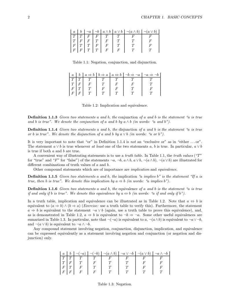
a b ¬a ¬b a ∧ b a ∨ b ¬(a ∧ b) ¬(a ∨ b)T T F F T T F FT F F T F T T FF T T F F T T FF F T T F F T T
Table 1.1: Negation, conjunction, and disjunction.
a b a⇒ b b⇒ a a⇔ b ¬b⇒ ¬a ¬a⇒ ¬bT T T T T T TT F F T F F TF T T F F T FF F T T T T T
Table 1.2: Implication and equivalence.
Definition 1.1.3 Given two statements a and b, the conjunction of a and b is the statement “a is trueand b is true”. We denote the conjunction of a and b by a ∧ b (in words: “a and b”).
Definition 1.1.4 Given two statements a and b, the disjunction of a and b is the statement “a is trueor b is true”. We denote the disjunction of a and b by a ∨ b (in words: “a or b”).
It is very important to note that “or” in Definition 1.1.4 is not an “exclusive or” as in “either . . . or”.The statement a ∨ b is true whenever at least one of the two statements a, b is true. In particular, a ∨ bis true if both a and b are true.A convenient way of illustrating statements is to use a truth table. In Table 1.1, the truth values (“T”
for “true” and “F” for “false”) of the statements ¬a, ¬b, a∧ b, a∨ b, ¬(a∧ b), ¬(a∨ b) are illustrated fordifferent combinations of truth values of a and b.Other compound statements which are of importance are implication and equivalence.
Definition 1.1.5 Given two statements a and b, the implication “a implies b” is the statement “If a istrue, then b is true”. We denote this implication by a⇒ b (in words: “a implies b”).
Definition 1.1.6 Given two statements a and b, the equivalence of a and b is the statement “a is trueif and only if b is true”. We denote this equivalence by a⇔ b (in words: “a if and only if b”).
In a truth table, implication and equivalence can be illustrated as in Table 1.2. Note that a ⇔ b isequivalent to (a⇒ b) ∧ (b⇒ a) (Exercise: use a truth table to verify this). Furthermore, the statementa ⇒ b is equivalent to the statement ¬a ∨ b (again, use a truth table to prove this equivalence), and,as is demonstrated in Table 1.2, a ⇒ b is equivalent to ¬b ⇒ ¬a. Some other useful equivalences aresumarized in Table 1.3. In particular, note that ¬(¬a) is equivalent to a, ¬(a∧b) is equivalent to ¬a∨¬b,and ¬(a ∨ b) is equivalent to ¬a ∧ ¬b.Any compound statement involving negation, conjunction, disjunction, implication, and equivalence
can be expressed equivalently as a statement involving negation and conjunction (or negation and dis-junction) only.
a b ¬(¬a) ¬(¬b) ¬(a ∧ b) ¬a ∨ ¬b ¬(a ∨ b) ¬a ∧ ¬bT T T T F F F FT F T F T T F FF T F T T T F FF F F F T T T T
Table 1.3: Negation.

1.1. ELEMENTARY LOGIC 3
The tools of elementary logic are useful in proving mathematical theorems. To illustrate that, weprovide a discussion of some common proof techniques.One possibility to prove that a statement is true is to use a direct proof. In the case of an implication,
a direct proof of the statement a⇒ b proceeds by assuming that a is true, and then showing that b mustnecessarily be true as well.Below is an example for a direct proof. Recall that a natural number (or positive integer) x is even if
and only if there exists a natural number n such that x = 2n. A natural number x is odd if and only ifthere exists a natural number m such that x = 2m− 1. Consider the following statements.
a: x is an even natural number and y is an even natural number,b: xy is an even natural number.
We now give a direct proof of the implication a⇒ b. Assume a is true. Because x and y are even, thereexist natural numbers n and m such that x = 2n and y = 2m. Therefore, xy = (2n)(2m) = 2(2nm) = 2r,where r := 2nm is a natural number (the notation := stands for “is defined by”). This means xy = 2rfor some natural number r, which proves that xy must be even. ‖(The symbol ‖ is used to denote the end of a proof.)Another possibility to prove that a statement is true is to show that its negation is false (it should
be clear from the equivalence of ¬(¬a) and a—see Table 1.3—that this is indeed equivalent to a directproof of a). This method of proof is called an indirect proof or a proof by contradiction.For example, consider the statements
a: x �= 0,b: There exists exactly one real number y such that xy = 1.
We prove a ⇒ b by contradiction, that is, we show that ¬(a⇒ b) must be false. Note that ¬(a ⇒ b) isequivalent to ¬(¬a ∨ b), which, in turn, is equivalent to a ∧ ¬b. Assume a ∧ ¬b is true (that is, a⇒ b isfalse). We will lead this assumption to a contradiction, which will prove that a⇒ b is true.Because a is true, x �= 0. If b is false, there are two possible cases. The first possible case is that
there exists no real number y such that xy = 1, and the second possibility is that there exist (at least)two different real numbers y and z such that xy = 1 and xz = 1. Consider the first case. Because x �= 0,we can choose y = 1/x. Clearly, xy = x(1/x) = 1, which is a contradiction. In the second case, we havexy = 1 ∧ xz = 1 ∧ y �= z. Because x �= 0, we can divide the two equations by x to obtain y = 1/x andz = 1/x. But this implies y = z, which is a contradiction to y �= z. Hence, in all possible cases, theassumption ¬(a ⇒ b) leads to a contradiction. Therefore, this assumption must be false, which meansthat a⇒ b is true. ‖Because, for any two statements a and b, a ⇔ b is equivalent to (a ⇒ b) ∧ (b ⇒ a), proving the
equivalence a⇔ b can be accomplished by proving the implications a⇒ b and b⇒ a.We conclude this section with another example of a mathematical proof, namely, the proof of the
quadratic formula. Consider the quadratic equation
x2 + px+ q = 0 (1.1)
where p and q are given real numbers. The following theorem provides conditions under which realnumbers x satisfying this equation exist, and shows how to find these solutions to (1.1).
Theorem 1.1.7 (i) The equation (1.1) has a real solution if and only if (p/2)2 ≥ q.(ii) A real number x is a solution to (1.1) if and only if[
x = −p2+
√(p2
)2− q]∨[x = −p
2−√(p2
)2− q]. (1.2)
Proof. (i) Adding (p/2)2 and subtracting q on both sides of (1.1), it follows that (1.1) is equivalent to
x2 + px+(p2
)2=(p2
)2− q
which, in turn, is equivalent to (x+p
2
)2=(p2
)2− q. (1.3)

4 CHAPTER 1. BASIC CONCEPTS
The left side of (1.3) is nonnegative. Therefore, (1.3) has a solution if and only if the right side of (1.3)is nonnegative as well, that is, if and only if (p/2)2 ≥ q.(ii) Because (1.3) is equivalent to (1.1), x is a solution to (1.1) if and only if x solves (1.3). Taking
square roots on both sides, we obtain[x+p
2=
√(p2
)2− q]∨[x+p
2= −√(p2
)2− q].
Subtracting p/2 from both sides, we obtain (1.2). ‖For example, consider the equation
x2 + 6x+ 5 = 0.
We have p = 6 and q = 5. Note that (p/2)2 − q = 4 ≥ 0, and therefore, the equation has a real solution.According to Theorem 1.1.7, a solution x must be such that
x = −3 +√(6
2
)2− 5
∨x = −3−
√(6
2
)2− 5
,
that is, the solutions are x = −1 and x = −5.As another example, consider
x2 + 2x+ 1 = 0.
We obtain (p/2)2 − q = 0, and it follows that we have the unique solution x = −1.Finally, consider
x2 + 2x+ 2 = 0.
We obtain (p/2)2 − q = −1 < 0, and therefore, this equation does not have a real solution.
1.2 Sets
As is the case for logical statements, sets are encountered frequently in everyday life. A set is a collectionof objects such as, for example, the set of all provinces of Canada, the set of all students registered inthis course, or the set of all natural numbers. The precise formal definition of a set that we will be usingis the following.
Definition 1.2.1 A set is a collection of objects such that, for each object under consideration, the objectis either in the set or not in the set, and each object appears at most once in a given set.
Note that, according to Definition 1.2.1, it is ruled out that an object belongs to a set and, at the sametime, does not belong to this set. Analogously to the assumption that a statement must be either trueor false (see Definition 1.1.1), such situations must be excluded in order to avoid logical inconsistencies.For a set A and an object x, we use the notation x ∈ A for “Object x is an element (or a member) of
A” (in the sense that x belongs to A). If x is not an element (a member) of A, we write x �∈ A. Clearly,the statement x �∈ A is equivalent to ¬(x ∈ A).There are different possibilities of describing a set. Some sets can be described by enumerating their
elements. For example, consider the sets
A := {Applied Health Sciences, Arts, Engineering, Environmental Studies,Mathematics, Science},
B := {2, 4, 6, 8, 10},IN := {1, 2, 3, 4, 5, . . .},Z := {0, 1,−1, 2,−2, 3,−3, . . .},∅ := {}.
The set ∅ is called the empty set (the set which contains no elements).There are sets that cannot be described by enumerating their elements, such as the set of real numbers.
Therefore, another method must be used to describe these sets. The second commonly used way ofdescribing a set is to enumerate the properties that are shared by its elements. For example, the sets A,B, IN, Z defined above can be described in terms of the properties of their members as

1.2. SETS 5
A = {x | x is a faculty of this university},B = {x | x is an even natural number between 1 and 10},IN = {x | x is a natural number},Z = {x | x is an integer}.
The symbol IN will be used throughout to denote the set of natural numbers. Z denotes the set ofintegers. Other important sets are
IN0 := {x | x ∈ Z ∧ x ≥ 0},IR := {x | x is a real number},IR+ := {x | x ∈ IR∧ x ≥ 0},IR++ := {x | x ∈ IR ∧ x > 0},Q := {x | x ∈ IR ∧ (∃p ∈ Z, q ∈ IN such that x = p/q)}.
Q is the set of rational numbers. The symbol ∃ stands for “there exists”. An example for a real numberthat is not a rational number is π = 3.141593 . . ..The following definitions describe some important relationships between sets.
Definition 1.2.2 For two sets A and B, A is a subset of B if and only if
x ∈ A⇒ x ∈ B.
We denote this subset relationship by A ⊆ B.
Therefore, A is a subset of B if and only if each element of A is also an element of B.An alternative way of formulating the statement x ∈ A⇒ x ∈ B is
∀x ∈ A, x ∈ B
where the symbol ∀ denotes “for all”. In general, implications such as x ∈ A⇒ b where A is a set and bis a statement can equivalently be formulated as
∀x ∈ A, b.
Sometimes, the notation B ⊇ A is used instead of A ⊆ B, which means “B is a superset of A”. Thestatements A ⊆ B and B ⊇ A are equivalent.Two sets are equal if and only if they contain the same elements. We can define this property of two
sets in terms of the subset relation.
Definition 1.2.3 Two sets A and B are equal if and only if (A ⊆ B) ∧ (B ⊆ A). In this case, we writeA = B.
Examples for subset relationships are
IN ⊆ Z, Z ⊆ Q, Q ⊆ IR, IR+ ⊆ IR, {1, 2, 4} ⊆ {1, 2, 3, 4}.
Intervals are important subsets of IR. We distinguish between non-degenerate and degenerate intervals.Let a, b ∈ IR be such that a < b. Then the following non-degenerate intervals can be defined.
[a, b] := {x | x ∈ IR ∧ (a ≤ x ≤ b)} (closed interval),(a, b) := {x | x ∈ IR∧ (a < x < b)} (open interval),[a, b) := {x | x ∈ IR ∧ (a ≤ x < b)} (half-open interval),(a, b] := {x | x ∈ IR ∧ (a < x ≤ b)} (half-open interval).
Using the symbols ∞ and −∞ for “infinity” and “minus infinity”, and letting a ∈ IR, the following setsare also non-degenerate intervals.
(−∞, a] := {x | x ∈ IR ∧ x ≤ a},(−∞, a) := {x | x ∈ IR∧ x < a},[a,∞) := {x | x ∈ IR∧ x ≥ a},(a,∞) := {x | x ∈ IR ∧ x > a}.

6 CHAPTER 1. BASIC CONCEPTS
�
�
�
�����
B
A
Figure 1.1: A ⊆ B.
In particular, IR+ = [0,∞) and IR++ = (0,∞) are non-degenerate intervals. Furthermore, IR is theinterval (−∞,∞). Degenerate intervals are either empty or contain one element only; that is, ∅ is adegenerate interval, and so are sets of the form {a} with a ∈ IR.If a set A is a subset of a set B and B, in turn, is a subset of a set C, then A must be a subset of C.
(This is the transitivity property of the relation ⊆.) Formally,
Theorem 1.2.4 For any three sets A, B, C,
(A ⊆ B) ∧ (B ⊆ C)⇒ A ⊆ C.
Proof. Suppose (A ⊆ B) ∧ (B ⊆ C). If A = ∅, A clearly is a subset of C (the empty set is a subset ofany set). Now suppose A �= ∅. We have to prove x ∈ A ⇒ x ∈ C. Let x ∈ A. Because A ⊆ B, x ∈ B.Because B ⊆ C, x ∈ C, which completes the proof. ‖The following definitions introduce some important set operations.
Definition 1.2.5 The intersection of two sets A and B is defined by
A ∩B := {x | x ∈ A ∧ x ∈ B}.
Definition 1.2.6 The union of two sets A and B is defined by
A ∪B := {x | x ∈ A ∨ x ∈ B}.
Two sets A and B are disjoint if and only if A ∩B = ∅, that is, two sets are disjoint if and only if theydo not have any common elements.
Definition 1.2.7 The difference between a set A and a set B is defined by
A \B := {x | x ∈ A ∧ x �∈ B}.
The set A \B is called “A without B” or “A minus B”.
Definition 1.2.8 The symmetric difference of two sets A and B is defined by
A�B := (A \B) ∪ (B \A).
Clearly, for any two sets A and B, we have A�B = B�A (prove this as an exercise).Sets can be illustrated diagramatically by using so-called Venn diagrams. For example, the subset
relation A ⊆ B can be illustrated as in Figure 1.1. The intersection A ∩ B and the union A ∪ B areillustrated in Figures 1.2 and 1.3. Finally, the difference A \B and the symmetric difference A�B areshown in Figures 1.4 and 1.5.As an example, consider the sets A = {1, 2, 3, 6} and B = {2, 3, 4, 5}. Then we obtain
A ∩B = {2, 3}, A ∪B = {1, 2, 3, 4, 5, 6}, A \B = {1, 6}, B \A = {4, 5}, A�B = {1, 4, 5, 6}.
For the applications of set theory discussed in this course, universal sets can be defined, where, fora given universal set, all sets under consideration are subsets of this universal set. For example, we willfrequently be concerned with subsets of IR, so that in these situations, IR can be considered the universalset. For obvious reasons, we will always assume that the universal set under consideration is nonempty.Given a universal set X and a set A ⊆ X, the complement of A in X can be defined.

1.2. SETS 7
�
�
�
�B
�
�
�
�A
���
���
���
Figure 1.2: A ∩B.
�
�
�
�B
�
�
�
�A
������
������
������ ��
��
��
��
��
��
��
��
�� �
���
����
���
�������
��
���
��
���
���
Figure 1.3: A ∪B.
�
�
�
�B
�
�
�
�A �
��
���
��
���
���
���
��
�����
Figure 1.4: A \B.
�
�
�
�B
�
�
�
�A �
��
���
��
���
���
���
��
�����
�� ���
��� �
�������
������
����
����
���
Figure 1.5: A�B.
X
����A
��
���
�����
������
��������
���������
����
�����
����
����������
����������
���������
��������
������
�����
���
��
��
��
��
���
��
��
��
Figure 1.6: A.

8 CHAPTER 1. BASIC CONCEPTS
Definition 1.2.9 Let X be a nonempty universal set, and let A ⊆ X. The complement of A in X isdefined by A := X \A.In a Venn diagram, the complement of A ⊆ X can be illustrated as in Figure 1.6.For example, if A = [a, b) ⊆ X = IR, the complement of A in IR is given by A = (−∞, a) ∪ [b,∞).
As another example, let X = IN and A = {x | x ∈ IN ∧ (x is odd)} ⊆ IN. We have A = {x | x ∈IN ∧ (x is even)}.The following theorem provides a few useful results concerning complements.
Theorem 1.2.10 Let X be a nonempty universal set, and let A ⊆ X.
(i) A = A,(ii) X = ∅,(iii) ∅ = X.
Proof. (i) A = X \A = {x | x ∈ X ∧x �∈ A} = {x | x ∈ X∧x �∈ {y | y �∈ A}} = {x | x ∈ X ∧x ∈ A} = A.(ii) We proceed by contradiction. Suppose X �= ∅. Then there exists y ∈ X. By definition, X = {x |
x ∈ X ∧ x �∈ X}. Therefore, y ∈ X ∧ y �∈ X. But this is a contradiction, because no object can be amember of a set and, at the same time, not be a member of this set.(iii) By way of contradiction, suppose ∅ �= X. Then there exists x ∈ X such that x �∈ ∅. But this
implies x ∈ ∅, which is a contradiction, because the empty set has no elements. ‖Part (i) of Theorem 1.2.10 states that, as one would expect, the complement of the complement of a
set A is the set A itself.Some important properties of set operations are summarized in the following theorem.
Theorem 1.2.11 Let A, B, C be sets.
(i.1) A ∩B = B ∩A,(i.2) A ∪B = B ∪A,(ii.1) A ∩ (B ∩ C) = (A ∩B) ∩C,(ii.2) A ∪ (B ∪ C) = (A ∪B) ∪C,(iii.1) A ∩ (B ∪ C) = (A ∩B) ∪ (A ∩ C),(iii.2) A ∪ (B ∩ C) = (A ∪B) ∩ (A ∪ C).
The proof of Theorem 1.2.11 is left as an exercise. Properties (i) are the commutative laws, (ii) are theassociative laws, and (iii) are the distributive laws of the set operations ∪ and ∩.Next, we introduce the Cartesian product of sets.
Definition 1.2.12 For two sets A and B, the Cartesian product of A and B is defined by
A× B := {(x, y) | x ∈ A ∧ y ∈ B}.
A×B is the set of all ordered pairs (x, y), the first component of which is a member of A, and the secondcomponent of which is an element of B. The term “ordered” is very important in the previous sentence.A pair (x, y) ∈ A × B is, in general, different from the pair (y, x). Note that nothing guarantees that(y, x) is even an element of A× B. Some examples for Cartesian products are given below.Let A = {1, 2, 4} and B = {2, 3}. Then
A ×B = {(1, 2), (1, 3), (2, 2), (2, 3), (4, 2), (4, 3)}.
As another example, let A = (1, 2) and B = [0, 1]. The Cartesian product of A and B is given by
A ×B = {(x, y) | (1 < x < 2) ∧ (0 ≤ y ≤ 1)}.
Finally, let A = {1} and B = [1, 2]. Then
A ×B = {(x, y) | x = 1 ∧ (1 ≤ y ≤ 2)}.
If A and B are subsets of IR, the Cartesian product A×B can be illustrated in a diagram. The aboveexamples are depicted in Figures 1.7 to 1.9.We can also form Cartesian products of more than two sets. The following definition introduces the
notion of an n-fold Cartesian product.

1.2. SETS 9
1 2 3 4 5x
1
2
3
4
5
y
uu uu uu
Figure 1.7: A×B, first example.
1 2 3 4 5x
1
2
3
4
5
y
�����
��
Figure 1.8: A ×B, second example.

10 CHAPTER 1. BASIC CONCEPTS
1 2 3 4 5 x
1
2
3
4
5
y
Figure 1.9: A×B, third example.
Definition 1.2.13 Let n ∈ IN. For n sets A1, A2, . . . , An, the Cartesian product of A1, A2, . . . , An isdefined by
A1 × A2 × . . .×An := {(x1, x2, . . . , xn) | xi ∈ Ai ∀i = 1, . . . , n}.
The elements of an n-fold Cartesian product are called ordered n-tuples (again, note that the order of thecomponents of an n-tuple is important).For example, if A1 = {1, 2}, A2 = {0, 1}, A3 = {1}, we obtain
A1 ×A2 × A3 = {(1, 0, 1), (1, 1, 1), (2, 0, 1), (2, 1, 1)}.
Of course, (some of) the sets A1, A2, . . . , An can be equal—Definitions 1.2.12 and 1.2.13 do not requirethe sets which define a Cartesian product to be distinct. For example, if A = {1, 2}, we can, for example,form the Cartesian products
A× A = {(1, 1), (1, 2), (2, 1), (2, 2)}
and
A× A× A = {(1, 1, 1), (1, 1, 2), (1, 2, 1), (1, 2, 2), (2, 1, 1), (2, 1, 2), (2, 2, 1), (2, 2, 2)}.
For simplicity, the n-fold Cartesian product of a set A is denoted by An, that is,
An := A× A× . . .× A︸ ︷︷ ︸n times
.
The most important Cartesian product in this course is the n-fold Cartesian product of IR, definedby
IRn := {(x1, x2, . . . , xn) | xi ∈ IR ∀i = 1, . . . , n}.
IRn is called the n-dimensional Euclidean space. (The term “space” is sometimes used for sets that havecertain structural properties.) The elements of IRn (ordered n-tuples of real numbers) are usually referredto as vectors—details will follow in Chapter 2.We conclude this section with some notation that will be used later on. For x = (x1, x2, . . . , xn) ∈ IRn,
we definen∑i=1
xi := x1 + x2 + . . .+ xn.
Therefore,∑ni=1 xi denotes the sum of the n numbers x1, x2, . . . , xn.

1.3. SETS OF REAL NUMBERS 11
1.3 Sets of Real Numbers
This section discusses some properties of subsets of IR that are of major importance in later chapters.First, we define neighborhoods of points in IR. Intuitively, a neighborhood of a point x0 ∈ IR is a set
of real numbers that are, in some sense, “close” to x0. In order to introduce neighborhoods formally, thedefinition of absolute values of real numbers is needed. For x ∈ IR, the absolute value of x is defined as
|x| :={
x if x ≥ 0−x if x < 0.
The definition of a neighborhood in IR is
Definition 1.3.1 For x0 ∈ IR and ε ∈ IR++, the ε-neighborhood of x0 is defined by
Uε(x0) := {x ∈ IR | |x− x0| < ε}.
Note that, in this definition, we used the formulation
. . . x ∈ IR | . . .
instead of. . . x | x ∈ IR ∧ . . .
in order to simplify notation. This notation will be used at times if one of the properties defining theelements of a set is the membership in some given set.|x−x0| is the distance between the points x and x0 in IR. According Definition 1.3.1, an ε-neighborhood
of x0 ∈ IR is the set of points x ∈ IR such that the distance between x and x0 is less than ε. Anε-neighborhood of x0 is a specific open interval containing x0—clearly, the neighborhood Uε(x0) can bewritten as
Uε(x0) = (x0 − ε, x0 + ε).
Neighborhoods can be used to define interior points of a set A ⊆ IR.
Definition 1.3.2 Let A ⊆ IR. x0 ∈ A is an interior point of A if and only if there exists ε ∈ IR++ suchthat Uε(x0) ⊆ A.
According to this definition, a point x0 ∈ A is an interior point of A if and only if there exists aneighborhood of x0 that is contained in A.For example, consider the set A = [0, 1). We will prove that all points x ∈ (0, 1) are interior points of
A, but the point 0 is not.First, let x0 ∈ [1/2, 1). Let ε := 1− x0. This implies x0− ε = 2x0− 1 ≥ 0 and x0+ ε = 1, and hence,
Uε(x0) = (x0 − ε, x0 + ε) ⊆ [0, 1) = A. Therefore, all points in [1/2, 1) are interior points of A.Now let x0 ∈ (0, 1/2). Define ε := x0. Then we have x0 − ε = 0 and x0 + ε = 2x0 < 1. Again,
Uε(x0) = (x0 − ε, x0 + ε) ⊆ [0, 1) = A. Hence, all points in the interval (0, 1/2) are interior points of A.To show that 0 is not an interior point of A, we proceed by contradiction. Suppose 0 is an interior
point of A = [0, 1). Then there exists ε ∈ IR++ such that Uε(0) = (−ε, ε) ⊆ [0, 1) = A. Let δ := ε/2.Then it follows that −ε < −δ < 0, and hence, −δ ∈ Uε(0). Because Uε(0) ⊆ A, this implies −δ ∈ A.Because −δ is negative, this is a contradiction to the definition of A.If all elements of a set A ⊆ IR are interior points, then A is called an open set in IR. Furthermore, if
the complement of a set A ⊆ IR is open in IR, then A is called closed in IR. Formally,
Definition 1.3.3 A set A ⊆ IR is open in IR if and only if
x ∈ A⇒ x is interior point of A.
Definition 1.3.4 A set A ⊆ IR is closed in IR if and only if A is open in IR.

12 CHAPTER 1. BASIC CONCEPTS
Openness and closedness can be defined in more abstract spaces than IR. However, for the purposes ofthis course, we can restrict attention to subsets of IR (and IRn, which will be discussed later on). Ifthere is no ambiguity concerning the universal set under consideration (in this course, IR or IRn), we willsometimes simply write “open” (respectively “closed”) instead of “open (respectively closed) in IR” (orin IRn).We have already seen that the set A = [0, 1) is not open in IR, because 0 is an element of A which
is not an interior point of A. To find out whether or not A is closed in IR, we have to consider thecomplement of A in IR. This complement is given by A = (−∞, 0) ∪ [1,∞). A is not an open set in IR,because the point 1 is not an interior point of A (prove this as an exercise—the proof is analogous to theproof that 0 is not an interior point of A). Therefore, A is not closed in IR. This example establishesthat there exist subsets of IR which are neither open nor closed in IR.Any open interval is an open set in IR (which justifies the terminology open intervals for these sets),
and all closed intervals are closed in IR. Furthermore, unions of disjoint open intervals are open, andunions of disjoint closed intervals are closed. IR itself is an open set. To show this, let x0 ∈ IR, and chooseany ε ∈ IR++. Clearly, (x0 − ε, x0 + ε) ⊆ IR, and therefore, all elements of IR are interior points of IR.The empty set is another example of an open set in IR. This is the case, because the empty set does
not contain any elements. According to Definition 1.3.3, openness of ∅ requires
x ∈ ∅ ⇒ x is interior point of ∅.
From Section 1.1, we know that the implication a⇒ b is equivalent to ¬a∨ b. Therefore, if a is false, theimplication is true. For any x ∈ IR, the statement x ∈ ∅ is false (because no object can be an element ofthe empty set). Consequently, the above implication is true for all x ∈ IR, which shows that ∅ is open inIR.Note that the openness of IR implies the closedness of ∅, and the openness of ∅ implies the closedness
of IR. Therefore, IR and ∅ are sets which are both open and closed in IR.We now define convex subsets of IR.
Definition 1.3.5 A set A ⊆ IR is convex if and only if
[λx+ (1 − λ)y] ∈ A ∀x, y ∈ A, ∀λ ∈ [0, 1].
Geometrically, a set A ⊆ IR is convex if, for any two points x and y in this set, all points on the linesegment joining x and y belong to A as well. A point λx + (1 − λ)y where λ ∈ [0, 1] is called a convexcombination of x and y. A convex combination of two points is simply a weighted average of these points.For example, if we set λ = 1/2, the corresponding convex combination is
1
2x+1
2y,
and for λ = 1/4, we obtain the convex combination
1
4x+3
4y.
The convex subsets of IR are easy to describe. All intervals (including IR itself) are convex (no matterwhether they are open, closed, or half-open), all sets consisting of a single point are convex, and theempty set is convex.For example, let A = [0, 1). To prove that A is convex, let x, y ∈ A. We have to show that any convex
combination of x and y must be in A. Let λ ∈ [0, 1]. Without loss of generality, suppose x ≤ y. Then itfollows that
λx + (1− λ)y ≥ λx+ (1− λ)x = xand
λx + (1− λ)y ≤ λy + (1− λ)y = y.Therefore, x ≤ λx + (1 − λ)y ≤ y. Because x and y are elements of A, x ≥ 0 and y < 1. Therefore,0 ≤ λx+ (1− λ)y < 1, which implies [λx+ (1− λ)y] ∈ A.An example of a subset of IR which is not convex is A = [0, 1]∪ {2}. Let x = 1, y = 2, and λ = 1/2.
Then x ∈ A and y ∈ A and λ ∈ [0, 1], but λx+ (1− λ)y = 3/2 �∈ A.The following definition introduces upper and lower bounds of subsets of IR.

1.4. FUNCTIONS 13
Definition 1.3.6 Let A ⊆ IR be nonempty, and let u, � ∈ IR.
(i) u is an upper bound of A if and only if x ≤ u for all x ∈ A.(ii) � is a lower bound of A if and only if x ≥ � for all x ∈ A.
A nonempty set A ⊆ IR is bounded from above (resp. bounded from below) if and only if it has an upper(resp. lower) bound. A nonempty set A ⊆ IR is bounded if and only if A has an upper bound and a lowerbound.Not all subsets of IR have upper or lower bounds. For example, the set IR+ = [0,∞) has no upper
bound. To show this, we proceed by contradiction. Suppose u ∈ IR is an upper bound of IR+. But IR+contains elements x such that x > u, which contradicts the assumption that u is an upper bound of IR+.On the other hand, IR+ is bounded from below—any number in the interval (−∞, 0] is a lower bound ofIR+.The above example shows that an upper bound or a lower bound need not be unique, if it exists.
Specific upper and lower bounds are introduced in the next definition.
Definition 1.3.7 Let A ⊆ IR be nonempty, and let u, � ∈ IR.(i) u is the least upper bound (the supremum) of A if and only if u is an upper bound of A and u ≤ u′
for all u′ ∈ IR that are upper bounds of A.(ii) � is the greatest lower bound (the infimum) of A if and only if � is a lower bound of A and � ≥ �′
for all �′ ∈ IR that are lower bounds of A.
Every nonempty subset of IR which has an upper (resp. lower) bound has a supremum (resp. an infimum).This is not necessarily the case if IR is replaced by some other universal set—for example, the set of rationalnumbers Q does not have this property.If a set A ⊆ IR has a supremum (resp. an infimum), the supremum (resp. infimum) is unique. Formally,
Theorem 1.3.8 Let A ⊆ IR be nonempty, and let u, u′, �, �′ ∈ IR.
(i) u is a supremum of A and u′ is a supremum of A ⇒ u = u′.(ii) � is an infimum of A and �′ is an infimum of A ⇒ � = �′.
Proof. (i) Let A ⊆ IR. Suppose u ∈ IR is a supremum of A and u′ ∈ IR is a supremum of A. This impliesthat u and u′ are upper bounds of A. By definition of a supremum, it follows that u ≤ u′ and u′ ≤ u,and therefore, u = u′.The proof of part (ii) is analogous. ‖Note that the above result justifies the terms “the” supremum and “the” infimum used in Definition
1.3.7. We will denote the supremum (resp. infimum) of A ⊆ IR by sup(A) (resp. inf(A)).Note that it is not required that the supremum (resp. infimum) of a set A ⊆ IR is itself an element
of A. For example, let A = [0, 1). As can be shown easily, the supremum and the infimum of A existand are given by sup(A) = 1 and inf(A) = 0. Therefore, inf(A) ∈ A, but sup(A) �∈ A. If the supremum(resp. infimum) of A ⊆ IR is an element of A, it is sometimes called the maximum (resp. minimum) of A,denoted by max(A) (resp. min(A)). Therefore, we can define the maximum and the minimum of a set by
Definition 1.3.9 Let A ⊆ IR be nonempty, and let u, � ∈ IR.
(i) u = max(A) if and only if u = sup(A) ∧ u ∈ A.(ii) � = min(A) if and only if � = inf(A) ∧ � ∈ A.
1.4 Functions
Given two sets A and B, a function that maps A into B assigns one element in B to each element inA. The use of functions is widespread (but not always recognized and explicitly declared as such). Forexample, giving final grades for a course to students is an example of establishing a function from the setof students registered in a course to the set of possible course grades. Each student is assigned exactlyone final grade. The formal definition of a function is
Definition 1.4.1 Let A and B be nonempty sets. If there exists a mechanism f that assigns exactly oneelement in B to each element in A, then f is called a function from A to B.

14 CHAPTER 1. BASIC CONCEPTS
A function from A to B is denoted by
f : A �→ B, x �→ y = f(x)
where y = f(x) ∈ B is the image of x ∈ A. A is the domain of the function f , B is the range of f . Theset
f(A) := {y ∈ B | ∃x ∈ A such that y = f(x)}is the image of A under f (sometimes also called the image of f). More generally, the image of S ⊆ Aunder f is defined as
f(S) := {y ∈ B | ∃x ∈ S such that y = f(x)}.Note that defining a function f involves two steps: First, the domain and the range of the function
have to be specified, and then, for each element x in the domain of the function, it has to be stated whichelement in the range of f is assigned to x according to f .Equality of functions is defined as
Definition 1.4.2 Two functions f1 : A1 �→ B1 and f2 : A2 �→ B2 are equal if and only if
(A1 = A2) ∧ (B1 = B2) ∧ (f1(x) = f2(x) ∀x ∈ A1).
Note that equality of two functions requires that their domains and their ranges are equal.To illustrate possible applications of functions, consider the above mentioned example. Suppose we
have a course in which six students are registered. For simplicity, we number the students from 1 to 6.The possible course grades are {A,B, C,D,F} (script letters are used in this example to avoid confusionwith the domain A and the range B of the function considered). An assignment of grades to studentscan be expressed as a function f : {1, 2, 3, 4, 5, 6} �→ {A,B, C,D,F}. For example, if students 1 and 3 getan A, student 2 gets a B, student 4 fails, and students 5 and 6 get a D, the function f is defined as
f : {1, 2, 3, 4, 5, 6} �→ {A,B, C,D,F}, x �→
A if x ∈ {1, 3}B if x = 2D if x ∈ {5, 6}F if x = 4.
(1.4)
The image of f is f(A) = {A,B,D,F}. As this example demonstrates, f(A) is not necessarily equal tothe range B—there may exist elements y ∈ B such that there exists no x ∈ A with y = f(x) (as is thecase for C ∈ B in the above example). Of course, by definition of f(A), we always have the relationshipf(A) ⊆ B.As another example, consider the function defined by
f : IR �→ IR, x �→ x2. (1.5)
The image of f is
f(IR) = {y ∈ IR | ∃x ∈ IR such that y = x2} = {y ∈ IR | y ≥ 0} = IR+.
Again, B = IR �= IR+ = f(IR) = f(A).Next, the graph of a function is defined.
Definition 1.4.3 The graph G of a function f : A �→ B is a subset of the Cartesian product A × B,defined as
G := {(x, y) | x ∈ A ∧ y = f(x)}.
In other words, the graph of a function f : A �→ B is the set of all pairs (x, f(x)), where x ∈ A. Forfunctions such that A ⊆ IR and B ⊆ IR, the graph is a useful tool to give a diagrammatic illustration ofthe function. For example, the graph of the function f defined in (1.5) is
G = {(x, y) | x ∈ IR ∧ y = x2}
and is illustrated in Figure 1.10.As mentioned before, the range of a function is not necessarily equal to the image of this function. In
the special case where f(A) = B, we say that the function f is surjective (or onto). We define

1.4. FUNCTIONS 15
-2 -1 0 1 2 x
1
2
3
4
5
y = f(x)
Figure 1.10: The graph of a function.
Definition 1.4.4 A function f : A �→ B is surjective (onto) if and only if f(A) = B.
A function f : A �→ B such that, for each y ∈ f(A), there exists exactly one x ∈ A with y = f(x) iscalled injective (or one-to-one). Formally,
Definition 1.4.5 A function f : A �→ B is injective (one-to-one) if and only if
∀x, y ∈ A, x �= y ⇒ f(x) �= f(y).
If a function is onto and one-to-one, the function is called bijective.
Definition 1.4.6 A function f : A �→ B is bijective if and only if f is surjective and injective.
As an example, consider the function f defined in (1.4). This function is not surjective, because thereexists no x ∈ {1, 2, 3, 4, 5, 6} such that f(x) = C. Furthermore, this function is not injective, because1 �= 3, but f(1) = f(3) = A.The function f defined in (1.5) is not surjective, because, for y = −1 ∈ B, there exists no x ∈ IR such
that f(x) = x2 = y. f is not injective, because, for example, f(1) = f(−1) = 1.As another example, define a function f by
f : IR �→ IR+, x �→ x2.
Note that this is not the same function as the one defined in (1.5), because it has a different range. Thatchoosing a different range indeed gives us a different function can be seen by noting that this function issurjective, whereas the one in the previous example is not. The function is not injective, and therefore,not bijective.Here is another example that illustrates the importance of defining the domain and the range properly.
Letf : IR+ �→ IR, x �→ x2.
This function is not surjective (note that its range is IR, but its image is IR+), but it is injective. To provethat, consider any x, y ∈ IR+ = A such that x �= y. Note that the domain of f is IR+, and therefore, xand y are nonnegative. Because x �= y, we can, without loss of generality, assume x > y. Because both xand y are nonnegative, it follows that x2 > y2, and therefore, f(x) = x2 �= y2 = f(y), which proves thatf is injective.As a final example, let
f : IR+ �→ IR+, x �→ x2.Now the domain and the range of f are given by IR+. For each y ∈ IR+ = B, there exists x ∈ IR+ = Asuch that y = f(x) (namely, x =
√y), which proves that f is onto. Furthermore, as in the previous

16 CHAPTER 1. BASIC CONCEPTS
example, f(x) �= f(y) whenever x, y ∈ IR+ = A and x �= y. Therefore, f is one-to-one, and hence,bijective.Bijective functions allow us to find, for each y ∈ B, a unique element x ∈ A such that y = f(x). This
suggests that a bijective function from A to B can be used to define another function with domain Band range A, which assigns each x ∈ A to its image under f . This motivates the following definition ofan inverse function.
Definition 1.4.7 Let f : A �→ B be bijective. The function defined by
f−1 : B �→ A, f(x) �→ x
is called the inverse function of f.
Note that an inverse function is not defined if f is not bijective.For example, consider the function
f : IR �→ IR, x �→ x3.
This function is bijective (Exercise: prove this), and consequently, its inverse function f−1 exists. Bydefinition of the inverse, we have, for all x ∈ IR, y ∈ IR,
f−1(y) = x⇔ y = x3 ⇔ y1/3 = x,
and therefore, the inverse of f is given by
f−1 : IR �→ IR, y �→ y1/3.
Two functions with appropriate domains and ranges can be combined to form a composite function.More precisely, composite functions are defined as
Definition 1.4.8 Suppose two functions f : A �→ B and g : B �→ C are given. The function
g ◦ f : A �→ C, x �→ g(f(x))
is the composite function of f and g.
An important property of the inverse function f−1 of a bijective function f is that its inverse is given byf . Hence, for a bijective function f : A �→ B, we have
f−1(f(x)) = x ∀x ∈ A
andf(f−1(y)) = y ∀y ∈ B.
The following definition introduces some important special cases of bijective functions, namely, per-mutations.
Definition 1.4.9 Let A be a finite subset of IN. A permutation of A is a bijective function π : A �→ A.
For example, a permutation of A = {1, 2, 3} is given by
π : {1, 2, 3} �→ {1, 2, 3}, x �→
1 if x = 12 if x = 33 if x = 2.
Other permutations of A are
π : {1, 2, 3} �→ {1, 2, 3}, x �→
1 if x = 22 if x = 33 if x = 1
(1.6)
and
π : {1, 2, 3} �→ {1, 2, 3}, x �→
1 if x = 32 if x = 23 if x = 1.

1.5. SEQUENCES OF REAL NUMBERS 17
A permutation can be used to change the numbering of objects. For example, if
π : {1, . . . , n} �→ {1, . . . , n}
is a permutation of {1, . . . , n} and x = (x1, . . . , xn) ∈ IRn, a renumbering of the components of x isobtained by applying the permutation π. The resulting vector is
xπ = (xπ(1), . . . , xπ(n)).
More specifically, if π is given by (1.6) and x = (x1, x2, x3) ∈ IR3, we obtain
xπ = (x3, x1, x2).
1.5 Sequences of Real Numbers
In addition to having some economic applications in their own right, sequences of real numbers arevery useful for the formulation of some properties of real-valued functions. This section provides abrief introduction to sequences of real numbers. We restrict attention to considerations that will be ofimportance for this course.A sequence of real numbers is a special case of a function as defined in the previous section, namely,
a function with the domain IN and the range IR.
Definition 1.5.1 A sequence of real numbers is a function a : IN �→ IR, n �→ a(n). To simplify notation,we will write an instead of a(n) for n ∈ IN, and use {an} to denote such a sequence.
More general sequences (not necessarily of real numbers) could be defined by allowing the range to be aset that is not necessarily equal to IR in the above definition. However, all sequences encountered in thischapter will be sequences of real numbers, and we will, for simplicity of presentation, refer to them as“sequences” and omit “of real numbers”. Sequences of elements of IRn will be discussed in Chapter 4.Here is an example of a sequence. Define
a : IN �→ IR, n �→ 1− 1n. (1.7)
The first few points in this sequence are
a1 = 0, a2 = 1/2, a3 = 2/3, a4 = 3/4, . . . .
Sequences also appear in economic problems. For example, suppose a given amount of money x ∈ IR++is deposited to a bank account, and there is a fixed rate of interest r ∈ IR++. After one year, the valueof this investment is x + rx = (1 + r)x. Assuming this amount is reinvested and the rate of interest isunchanged, the value after two years is (1 + r)x + r(1 + r)x = (1 + r)(1 + r)x = x(1 + r)2. In general,after n ∈ IN years, the value of the investment is x(1 + r)n. These values of the investment in differentyears can be expressed as a sequence, namely, the sequence {an}, where
an = x(1 + r)n ∀n ∈ IN.
This is a special case of a geometric sequence.
Definition 1.5.2 A sequence {an} is a geometric sequence if and only if there exists q ∈ IR such that
an+1 = qan ∀n ∈ IN.
A geometric sequence has a quite simple structure in the sense that all elements of the sequence canbe derived from the first element of the sequence, given the number q ∈ IR. This is the case because,according to Definition 1.5.2, a2 = qa1, a3 = qa2 = q
2a1 and, for n ∈ IN with n ≥ 2, an = qn−1a1. Theabove example of interest accumulation is a geometric sequence, where q = 1 + r and a1 = qx.It is often important to analyze the behaviour of a sequence as n becomes, loosely speaking, “large”.
To formalize this notion more precisely, we introduce the following definition.

18 CHAPTER 1. BASIC CONCEPTS
Definition 1.5.3 (i) A sequence {an} converges to α ∈ IR if and only if
∀ε ∈ IR++, ∃n0 ∈ IN such that an ∈ Uε(α) ∀n ≥ n0.
(ii) If {an} converges to α ∈ IR, α is the limit of {an}, and we write
limn→∞
an = α.
Recall that Uε(α) is the ε-neighborhood of α ∈ IR, where ε ∈ IR++. Therefore, the statement “an ∈ Uε(α)”is equivalent to “|an − α| < ε”.In words, {an} converges to α ∈ IR if and only if, for any ε ∈ IR++, at most a finite number of elements
of {an} are outside the ε-neighborhood of α.To illustrate this definition, consider again the sequence defined in (1.7). We prove that this sequence
converges to the limit 1. In order to do so, we show that, for all ε ∈ IR++, there exists n0 ∈ IN such that|an − 1| < ε for all n ≥ n0. For any ε ∈ IR++, choose n0 ∈ IN such that n0 > 1/ε. For n ≥ n0, it followsthat n > 1/ε, and therefore,
ε >1
n= |1− 1
n− 1| = |an − 1|,
which shows that the sequence {an} converges to the limit α = 1.The following terminology will be used.
Definition 1.5.4 A sequence {an} is convergent if and only if there exists α ∈ IR such that
limn→∞
an = α.
A sequence {an} is divergent if and only if {an} is not convergent.
Here is an example of a divergent sequence. Define {an} by
an = n ∀n ∈ N. (1.8)
That this sequence diverges can be shown by contradiction. Suppose {an} is convergent. Then thereexists α ∈ IR such that limn→∞ an = α. Therefore, for any ε ∈ IR++, there exists n0 ∈ IN such that
|n− α| < ε ∀n ≥ n0. (1.9)
Let n1 ∈ IN be such that n1 > α+ ε. Then n1 − α > ε, and therefore,
|n− α| = n− α > ε ∀n ≥ n1. (1.10)
Let n2 ∈ IN be such that n2 ≥ n0 and n2 ≥ n1. Then (1.9) implies |n2 − α| < ε, and (1.10) implies|n2 − α| > ε, which is a contradiction.Two special cases of divergence, defined below, are of particular importance.
Definition 1.5.5 A sequence {an} diverges to ∞ if and only if
∀c ∈ IR, ∃n0 ∈ IN such that an ≥ c ∀n ≥ n0.
Definition 1.5.6 A sequence {an} diverges to −∞ if and only if
∀c ∈ IR, ∃n0 ∈ IN such that an ≤ c ∀n ≥ n0.
For example, the sequence {an} defined in (1.8) diverges to ∞ (Exercise: provide a proof).Note that there are divergent sequences which do not diverge to ∞ or −∞. A divergent sequence
which does not diverge to ∞ or −∞ is said to oscillate. For example, consider the sequence {an} definedby
an =
{0 if n is even1 if n is odd.
(1.11)
As an exercise, prove that this sequence oscillates.

1.5. SEQUENCES OF REAL NUMBERS 19
For a sequence {an} and α ∈ IR ∪ {−∞,∞}, we will sometimes use the notation
an −→ α
if α ∈ IR and {an} converges to α, or if α ∈ {−∞,∞} and {an} diverges to α.In Definition 1.5.3, we referred to α as “the” limit of {an}, if {an} converges to α. This terminology is
justified, because a sequence cannot have more than one limit. That is, the limit of a convergent sequenceis unique, as stated in the following theorem.
Theorem 1.5.7 Let {an} be a sequence, and let α, β ∈ IR. If limn→∞ an = α and limn→∞ an = β, thenα = β.
Proof. By way of contradiction, assume
( limn→∞
an = α) ∧ ( limn→∞
an = β) ∧ α �= β.
Without loss of generality, suppose α < β. Define
ε :=β − α2> 0.
Then it follows that
Uε(α) =(α− β + α+ β
2,α+ β
2
)and
Uε(β) =(α+ β
2,α+ β
2+ β − α
).
Therefore,Uε(α) ∩ Uε(β) = ∅. (1.12)
Because limn→∞ an = α, there exists n0 ∈ IN such that an ∈ Uε(α) for all n ≥ n0. Analogously, becauselimn→∞ an = β, there exists n1 ∈ IN such that an ∈ Uε(β) for all n ≥ n1. Let n2 ∈ IN be such thatn2 ≥ n0 and n2 ≥ n1. Then
an ∈ Uε(α) ∧ an ∈ Uε(β) ∀n ≥ n2,
which is equivalent to an ∈ Uε(α) ∩ Uε(β) for all n ≥ n2, a contradiction to (1.12). ‖The convergence of some sequences can be established by showing that they have certain properties.
We define
Definition 1.5.8
(i) A sequence {an} is monotone nondecreasing ⇔ an+1 ≥ an ∀n ∈ IN,(ii) A sequence {an} is monotone nonincreasing ⇔ an+1 ≤ an ∀n ∈ IN.
Definition 1.5.9
(i) A sequence {an} is bounded from above⇔ ∃c ∈ IR such that an ≤ c ∀n ∈ IN,(ii) A sequence {an} is bounded from below⇔ ∃c ∈ IR such that an ≥ c ∀n ∈ IN,(iii) A sequence {an} is bounded ⇔ {an} is bounded from above and from below.
For example, consider the sequence {an} defined in (1.7). This sequence is monotone nondecreasing,because
an+1 = 1−1
n + 1≥ 1− 1
n= an ∀n ∈ IN.
Furthermore, {an} is bounded, because 0 ≤ an ≤ 1 for all n ∈ IN.There are some important relationships between convergent, monotone, and bounded sequences. First,
we show that a convergent sequence must be bounded.
Theorem 1.5.10 Let {an} be a sequence. If {an} is convergent, then {an} is bounded.

20 CHAPTER 1. BASIC CONCEPTS
Proof. Suppose {an} is convergent with limit α ∈ IR. Let ε = 1. Then there exists n0 ∈ IN such that|an − α| < 1 ∀n ≥ n0.
Define
N1 := {n ∈ IN | n > n0 ∧ an ≥ α},N2 := {n ∈ IN | n > n0 ∧ an < α}.
Then it follows that
an < α+ 1 ∀n ∈ N1, (1.13)
an > α− 1 ∀n ∈ N2. (1.14)
Now define
c1 := max({a1, . . . , an0, α+ 1}),c2 := min({a1, . . . , an0, α− 1}).
(Clearly, c1 and c2 are well-defined, because a finite set of real numbers must have a maximum and aminimum.) This, together with (1.13) and (1.14), implies
c2 ≤ an ≤ c1 ∀n ∈ N,which proves that {an} is bounded. ‖Boundedness of a sequence does not imply the convergence of this sequence. For example, the se-
quence {an} defined in (1.11) is bounded (because 0 ≤ an ≤ 1 for all n ∈ IN), but it is not convergent.However, boundedness from above (resp. below) together with monotone nondecreasingness (resp. nonin-creasingness) together imply that a sequence is convergent. This result provides a criterion that is oftenvery useful when it is to be determined whether a sequence is convergent. The theorem below states thisresult formally.
Theorem 1.5.11 Let {an} be a sequence.(i) {an} is monotone nondecreasing and bounded from above ⇒
{an} is convergent with limit sup({an | n ∈ IN}).(ii) {an} is monotone nonincreasing and bounded from below ⇒
{an} is convergent with limit inf({an | n ∈ IN}).Proof. (i) Suppose {an} is bounded from above and monotone nondecreasing. Boundedness from aboveof {an} is equivalent to the boundedness from above of the set {an | n ∈ IN}. Therefore, sup({an | n ∈ IN})exists. Letting α = sup({an | n ∈ IN}), we have an ≤ α for all n ∈ IN. Next, we show
∀ε ∈ IR++, ∃n0 ∈ IN such that α− an0 < ε. (1.15)
Suppose this is not the case. Then there exists ε ∈ IR++ such that α−an ≥ ε for all n ∈ IN. Equivalently,α − ε ≥ an for all n ∈ IN, which means that α − ε is an upper bound of {an | n ∈ IN}. Becauseα − ε < α, this contradicts the definition of α as the supremum of this set. Therefore, (1.15) is true.This implies α− ε < an0 . Because {an} is monotone nondecreasing, an ≥ an0 for all n ≥ n0. Therefore,α− ε < an0 ≤ an for all n ≥ n0, which implies
α− an < ε ∀n ≥ n0. (1.16)
Because an ≤ α for all n ∈ IN, (1.16) is equivalent to|an − α| < ε ∀n ≥ n0,
which proves that α is the limit of {an}.The proof of part (ii) of the theorem is analogous. ‖The results below show how the limits of sums, products, and ratios of convergent sequences can be
obtained. The proofs of these theorems are left as exercises.
Theorem 1.5.12 Let {an}, {bn} be sequences, and let α, β ∈ IR. If limn→∞ an = α and limn→∞ bn = β,then limn→∞(an + bn) = α+ β and limn→∞(anbn) = αβ.
Theorem 1.5.13 Let {an}, {bn} be sequences, and let α, β ∈ IR. Furthermore, let bn �= 0 for all n ∈ INand β �= 0. If limn→∞ an = α and limn→∞ bn = β, then limn→∞(an/bn) = α/β.

Chapter 2
Linear Algebra
2.1 Vectors
In Chapter 1, we introduced elements of the space IRn as ordered n-tuples (x1, . . . , xn), where xi ∈ IRfor all i = 1, . . . , n. Geometrically, we can think of x ∈ IRn as a point in the n-dimensional space. Forexample, for n = 2, the point x = (1, 2) ∈ IR2 can be represented by a point in the two-dimensionalcoordinate system with the coordinates 1 and 2.Another possibility is to think of x ∈ IRn as a parametrization of a vector in IRn. We can visualize the
vector x ∈ IRn as an “arrow” starting at the origin 0 = (0, . . . , 0) ∈ IRn which “points” at x = (x1, . . . , xn).For example, the vector x = (1, 2) ∈ IR2 can be represented as in Figure 2.1.For some of our applications, it is important whether the components of a vector in IRn are arranged
in a column or in a row. A column vector in IRn is written as
x =
x1...xn
∈ IRn,
and the corresponding row vector (the vector with the same elements as x, but arranged in a row) is
x′ = (x1, . . . , xn) ∈ IRn.
The notation ′ stands for “transpose”. For example, the transpose of
x =
(12
)∈ IR2
is x′ = (1, 2). If x is a column vector, then its transpose is a row vector. The transpose of the transposeof a vector x ∈ IRn is the vector x itself, that is, (x′)′ = x. For simplicity, we will omit the ′ for rowvectors whenever it is of no importance whether x ∈ IRn is to be treated as a column vector or a rowvector. It should be kept in mind, though, that for some applications, this distinction is of importance.The following operations can be applied to vectors.
Definition 2.1.1 Let n ∈ IN, and let x, y ∈ IRn. The sum of x and y is defined by
x+ y :=
x1 + y1...xn + yn
.
Definition 2.1.2 Let n ∈ IN, let α ∈ IR, and let x ∈ IRn. The product of α and x is defined by
αx :=
αx1...αxn
.
21

22 CHAPTER 2. LINEAR ALGEBRA
1 2 3 4 5 x1
1
2
3
4
5
x2
�������
Figure 2.1: The vector x = (1, 2).
1 2 3 4 5x1
1
2
3
4
5
x2
���������
����
����
�������������
x
y
x+ y
Figure 2.2: Vector addition.
The operation described in Definition 2.1.1 is called vector addition, the operation introduced in Definition2.1.2 is called scalar multiplication.Vector addition and scalar multiplication have very intuitive geometric interpretations. Consider, for
example, x = (1, 2) ∈ IR2 and y = (3, 1) ∈ IR2. Then we obtain x+y = (1+3, 2+1) = (4, 3). This vectoraddition is illustrated in Figure 2.2.Now consider x = (1, 2) ∈ IR2 and α = 2. We obtain αx = (2 · 1, 2 · 2) = (2, 4), which is illustrated in
Figure 2.3.Geometrically, the vector 2x points in the same direction as x ∈ IRn, but is twice as long (we will
discuss the notion of the “length” of a vector in more detail below).Using vector addition and scalar multiplication, we can define the operation vector subtraction.
Definition 2.1.3 Let n ∈ IN, and let x, y ∈ IRn. The difference of x and y is defined by
x− y := x+ (−1)y.
The following theorem summarizes some properties of vector addition and scalar multiplication.
Theorem 2.1.4 Let n ∈ IN, let α, β ∈ IR, and let x, y, z ∈ IRn.

2.1. VECTORS 23
1 2 3 4 5 x1
1
2
3
4
5
x2
�������
x
�������������
2x
Figure 2.3: Scalar multiplication.
(i) x+ y = y + x,(ii) (x+ y) + z = x+ (y + z),(iii) α(βx) = (αβ)x,(iv) (α+ β)x = αx+ βx,(v) α(x+ y) = αx+ αy.
The proof of this theorem is left as an exercise.Vector addition and scalar multiplication yield new vectors in IRn. The operation introduced in the
following definition assigns a real number to a pair of vectors.
Definition 2.1.5 Let n ∈ IN, and let x, y ∈ IRn. The inner product of x and y is defined by
xy :=n∑i=1
xiyi.
The inner product of two vectors is used frequently in economic models. For example, if x ∈ IRn+ representsa commodity bundle and p ∈ IRn++ denotes a price vector, the inner product px =
∑ni=1 pixi is the value
of the commodity bundle at these prices.The inner product has the following properties.
Theorem 2.1.6 Let n ∈ IN, let α ∈ IR, and let x, y, z ∈ IRn.
(i) xy = yx,(ii) xx ≥ 0,(iii) xx = 0⇔ x = 0,(iv) (x+ y)z = xz + yz,(v) (αx)y = α(xy).
Again, the proof of this theorem is left as an exercise.Of special importance are the so-called unit vectors in IRn. For i ∈ {1, . . . , n}, the ith unit vector is
defined by
eij :=
{0 if j �= i1 if j = i
∀j = 1, . . . , n.
For example, for n = 2, e1 = (1, 0) and e2 = (0, 1). See Figure 2.4.We now define the Euclidean norm of a vector.

24 CHAPTER 2. LINEAR ALGEBRA
1 2 3 4 5 x1
1
2
3
4
5
x2
�
�e1
e2
Figure 2.4: Unit vectors.
Definition 2.1.7 Let n ∈ IN, and let x ∈ IRn. The Euclidean norm of x is defined by
‖x‖ :=√xx =
√√√√ n∑i=1
x2i .
Because the Euclidean norm is the only norm considered in this chapter, we will refer to ‖x‖ simply asthe norm of x ∈ IRn. Geometrically, the norm of a vector can be interpreted as a measure of its length.For example, let x = (1, 2) ∈ IR2. Then
‖x‖ =√1 · 1 + 2 · 2 =
√5.
Clearly, ‖ei‖ = 1 for the unit vector ei ∈ IRn.Based on the Euclidean norm, we can define the Euclidean distance of two vectors x, y ∈ IRn as the
norm of the difference x− y.Definition 2.1.8 Let n ∈ IN, and let x, y ∈ IRn. The Euclidean distance of x and y is defined by
d(x, y) := ‖x− y‖.
Again, we will omit the term “Euclidean”, because the above defined distance is the only notion of distanceused in this chapter. See Chapter 4 for a more detailed discussion of distance functions for vectors. Forn = 1, we obtain the usual norm and distance used for real numbers. For x ∈ IR, ‖x‖ =
√x2 = |x|, and
for x, y ∈ IR, d(x, y) = ‖x− y‖ = |x− y|.For many applications discussed in this course, the question whether or not some vectors are linearly
independent is of great importance. Before defining the terms “linear (in)dependence” precisely, we haveto introduce linear combinations of vectors.
Definition 2.1.9 Let m, n ∈ IN, and let x1, . . . , xm, y ∈ IRn. y is a linear combination of x1, . . . , xm ifand only if there exist α1, . . . , αm ∈ IR such that
y =m∑j=1
αjxj.
For example, consider the vectors x1 = (1, 2), x2 = (0, 1), x3 = (5,−1), y = (−9/2, 5) in IR2. y is a linearcombination of x1, x2, x3, because, with α1 = 1/2, α2 = 3, α3 = −1, we obtain
y = α1x1 + α2x
2 + α3x3.
Note that any vector x ∈ IRn can be expressed as a linear combination of the unit vectors e1, . . . , en—simply choose αi = xi for all i = 1, . . . , n to verify this.Linear (in)dependence of vectors is defined as

2.1. VECTORS 25
Definition 2.1.10 Let m, n ∈ IN, and let x1, . . .xm ∈ IRn. The vectors x1, . . . , xm are linearly indepen-dent if and only if
m∑j=1
αjxj = 0⇒ αj = 0 ∀j = 1, . . . , m.
The vectors x1, . . . xm are linearly dependent if and only if they are not linearly independent.
Linear independence of x1, . . . , xm requires that the only possibility to choose α1, . . . , αm ∈ IR such that∑mj=1 αjx
j = 0 is to choose α1 = . . . = αm = 0. Clearly, the vectors x1, . . . , xm are linearly dependent if
and only if there exist α1, . . . , αm ∈ IR such thatm∑j=1
αjxj = 0 ∧ (∃k ∈ {1, . . . , m} such that αk �= 0).
As an example, consider the vectors x1 = (2, 1), x2 = (1, 0). To check whether these vectors are linearlyindependent, we have to consider the equation
α1
(21
)+ α2
(10
)=
(00
). (2.1)
(2.1) is equivalent to2α1 + α2 = 0 ∧ α1 = 0. (2.2)
By (2.2), we must have α1 = 0, and therefore, α2 = 0 in order to satisfy (2.1). Hence, the only possibilityto satisfy (2.1) is to choose α1 = α2 = 0, which means that the two vectors are linearly independent.Another example for a set of linearly independent vectors is the set of unit vectors {e1, . . . , en} in IRn.
Clearly, the equationn∑j=1
αjej = 0
is equivalent to
α1
10...0
+ . . .+ αn
0...01
=
0...0
,
which requires αj = 0 for all j = 1, . . . , n. For a single vector x ∈ IRn, it is not very hard to find outwhether the vector is linearly dependent or independent. This is shown in
Theorem 2.1.11 Let n ∈ IN, and let x ∈ IRn. x is linearly independent if and only if x �= 0.
Proof. Let x = 0. Then any α ∈ IR satisfies
αx = 0. (2.3)
Therefore, there exists α �= 0 satisfying (2.3), which shows that 0 is linearly dependent.Now let x �= 0. Then there exists k ∈ {1, . . . , n} such that xk �= 0. To satisfy
α
x1...xn
=
0...0
, (2.4)
we must, in particular, have αxk = 0. Because xk �= 0, the only possibility to satisfy (2.4) is to chooseα = 0. Therefore, x is linearly independent. ‖The following theorem provides an alternative formulation of linear dependence for m ≥ 2 vectors.
Theorem 2.1.12 Let n,m ∈ IN with m ≥ 2, and let x1, . . . , xm ∈ IRn. The vectors x1, . . . , xm arelinearly dependent if and only if (at least) one of these vectors is a linear combination of the remainingvectors.

26 CHAPTER 2. LINEAR ALGEBRA
Proof. “Only if”: Suppose x1, . . . , xm are linearly dependent. Then there exist α1, . . .αm ∈ IR such that
m∑j=1
αjxj = 0 (2.5)
and there exists k ∈ {1, . . . , m} such that αk �= 0. Without loss of generality, suppose k = m. Becauseαm �= 0, we can divide (2.5) by αm to obtain
m∑j=1
αj
αmxj = 0
or, equivalently,
xm =m−1∑j=1
βjxj,
where βj := −αj/αm for all j = 1, . . . , m− 1. But this means that xm is a linear combination of theremaining vectors.
“If”: Suppose one of the vectors x1, . . . , xm is a linear combination of the remaining vectors. Withoutloss of generality, suppose xm is this vector. Then there exist α1, . . . , αm−1 ∈ IR such that
xm =m−1∑j=1
αjxj .
Defining αm := −1, this is equivalent tom∑j=1
αjxj = 0.
Because αm �= 0, this implies that the vectors x1, . . . , xm are linearly dependent. ‖Further results concerning linear (in)dependence will follow later in this chapter, once matrices and
the solution of systems of linear equations have been discussed.
2.2 Matrices
Matrices are arrays of real numbers. The formal definition is
Definition 2.2.1 Let m, n ∈ IN. An m× n matrix is an array
A = (aij) =
a11 a12 . . . a1na21 a22 . . . a2n...
......
am1 am2 . . . amn
where aij ∈ IR for all i = 1, . . . , m, j = 1, . . . , n.
Therefore, an m× n matrix is an array of real numbers with m rows and n columns. An m× n matrixsuch that m = n is called a square matrix, that is, a square matrix has the same number of rows andcolumns.
Equality of two matrices is defined as
Definition 2.2.2 Let m, n, q, r ∈ IN. Furthermore, let A = (aij) be an m× n matrix, and let B = (bij)be a q × r matrix. A and B are equal if and only if
(m = q) ∧ (n = r) ∧ (aij = bij ∀i = 1, . . . , m, ∀j = 1, . . . , n).

2.2. MATRICES 27
Vectors are special cases of matrices. A column vector
x =
x1...xn
∈ IRn
is an n× 1 matrix, and a row vector x′ = (x1, . . . , xn) ∈ IRn is a 1 × n matrix. We can also think of anm× n matrix as an ordered n-tuple of m-dimensional column vectors
a11...am1
. . .
a1n
...amn
or as an ordered m-tuple of n-dimensional row vectors
(a11, . . . , a1n)...
(am1, . . . , amn).
The transpose of a matrix is defined as
Definition 2.2.3 Let m, n ∈ IN, and let A be an m× n matrix. The transpose of A is defined by
A′ :=
a11 a21 . . . am1a12 a22 . . . am2...
......
a1n a2n . . . amn
.
Clearly, if A is an m× n matrix, A′ is an n×m matrix. The transpose of A is obtained by interchangingthe roles of rows and columns. For i = 1, . . . , m and j = 1, . . . , n, the ith row of A is the ith column ofA′, and the jth column of A is the jth row of A′. For example, the transpose of the 2× 3 matrix
A =
(3 −1 02 0 1
)is the 3× 2 matrix
A′ =
3 2−1 00 1
.
The transpose of the transpose of a matrix A is the matrix A itself, that is, for any matrix A, (A′)′ = A.Symmetric square matrices will play an important role in this course. We define
Definition 2.2.4 Let n ∈ IN. An n × n matrix A is symmetric if and only if A′ = A.
Note that symmetry is defined only for square matrices. For example, the 2× 2 matrix
A =
(1 22 0
)is symmetric, because
A′ =
(1 22 0
)= A.
On the other hand, the 2× 2 matrixB =
(1 2−2 0
)is not symmetric, because
B′ =
(1 −22 0
)�= B.
Now we will introduce some important matrix operations. First, we define matrix addition.

28 CHAPTER 2. LINEAR ALGEBRA
Definition 2.2.5 Let m, n ∈ IN, and let A = (aij) and B = (bij) be m× n matrices. The sum of A andB is defined by
A+ B := (aij + bij) =
a11 + b11 a12 + b12 . . . a1n + b1na21 + b21 a22 + b22 . . . a2n + b2n...
......
am1 + bm1 am2 + bm2 . . . amn + bmn
.
Note that the sum A+ B is defined only for matrices of the same type, that is, A and B must have thesame number of rows and the same number of columns. As examples, consider the 2× 3 matrices
A =
(2 1 03 0 −1
), B =
(1 0 00 2 2
).
The sum of theses two matrices is
A +B =
(3 1 03 2 1
).
Next, scalar multiplication is defined.
Definition 2.2.6 Let m, n ∈ IN, and let A = (aij) be an m× n matrix. Furthermore, let α ∈ IR. Theproduct of α and A is defined by
αA := (αaij) =
αa11 αa12 . . . αa1nαa21 αa22 . . . αa2n...
......
αam1 αam2 . . . αamn
.
For example, let α = −2 and
A =
0 −21 25 0
.
Then
αA =
0 4−2 −4−10 0
.
The following theorem summarizes some properties of matrix addition and scalar multiplication (notethe similarity to Theorem 2.1.4).
Theorem 2.2.7 Let m, n ∈ IN, and let A, B, C be m× n matrices. Furthermore, let α, β ∈ IR.
(i) A +B = B +A,(ii) (A +B) +C = A + (B + C),(iii) α(βA) = (αβ)A,(iv) (α+ β)A = αA+ βA,(v) α(A+B) = αA + αB.
As an exercise, prove this theorem.The multiplication of two matrices is only defined if the matrices satisfy a conformability condition
for matrix multiplication. In particular, the matrix product AB is defined only if the number of columnsin A is equal to the number of rows in B.
Definition 2.2.8 Let m, n, r ∈ IN. Furthermore, let A = (aij) be an m× n matrix and let B = (bij) bean n × r matrix. The matrix product AB is defined by
AB :=
(n∑k=1
aikbkj
)=
∑nk=1 a1kbk1
∑nk=1 a1kbk2 . . .
∑nk=1 a1kbkr∑n
k=1 a2kbk1∑nk=1 a2kbk2 . . .
∑nk=1 a2kbkr
......
...∑nk=1 amkbk1
∑nk=1 amkbk2 . . .
∑nk=1 amkbkr
.
2.2. MATRICES 29
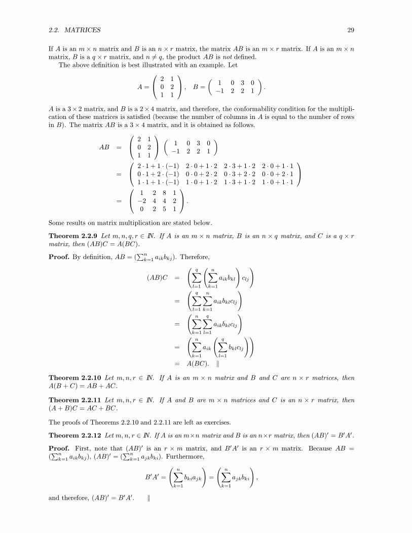
If A is an m× n matrix and B is an n × r matrix, the matrix AB is an m× r matrix. If A is an m× nmatrix, B is a q × r matrix, and n �= q, the product AB is not defined.The above definition is best illustrated with an example. Let
A =
2 10 21 1
, B = ( 1 0 3 0
−1 2 2 1
).
A is a 3× 2 matrix, and B is a 2× 4 matrix, and therefore, the conformability condition for the multipli-cation of these matrices is satisfied (because the number of columns in A is equal to the number of rowsin B). The matrix AB is a 3× 4 matrix, and it is obtained as follows.
AB =
2 10 21 1
( 1 0 3 0
−1 2 2 1
)
=
2 · 1 + 1 · (−1) 2 · 0 + 1 · 2 2 · 3 + 1 · 2 2 · 0 + 1 · 10 · 1 + 2 · (−1) 0 · 0 + 2 · 2 0 · 3 + 2 · 2 0 · 0 + 2 · 11 · 1 + 1 · (−1) 1 · 0 + 1 · 2 1 · 3 + 1 · 2 1 · 0 + 1 · 1
=
1 2 8 1−2 4 4 20 2 5 1
.
Some results on matrix multiplication are stated below.
Theorem 2.2.9 Let m, n, q, r ∈ IN. If A is an m × n matrix, B is an n × q matrix, and C is a q × rmatrix, then (AB)C = A(BC).
Proof. By definition, AB = (∑nk=1 aikbkj). Therefore,
(AB)C =
(q∑l=1
(n∑k=1
aikbkl
)clj
)
=
(q∑l=1
n∑k=1
aikbklclj
)
=
(n∑k=1
q∑l=1
aikbklclj
)
=
(n∑k=1
aik
(q∑l=1
bklclj
))
= A(BC). ‖
Theorem 2.2.10 Let m, n, r ∈ IN. If A is an m × n matrix and B and C are n × r matrices, thenA(B + C) = AB +AC.
Theorem 2.2.11 Let m, n, r ∈ IN. If A and B are m × n matrices and C is an n × r matrix, then(A +B)C = AC +BC.
The proofs of Theorems 2.2.10 and 2.2.11 are left as exercises.
Theorem 2.2.12 Let m, n, r ∈ IN. If A is an m×n matrix and B is an n×r matrix, then (AB)′ = B′A′.
Proof. First, note that (AB)′ is an r × m matrix, and B′A′ is an r × m matrix. Because AB =(∑nk=1 aikbkj), (AB)
′ = (∑nk=1 ajkbki). Furthermore,
B′A′ =
(n∑k=1
bkiajk
)=
(n∑k=1
ajkbki
),
and therefore, (AB)′ = B′A′. ‖

30 CHAPTER 2. LINEAR ALGEBRA
Theorem 2.2.9 describes the associative laws of matrix multiplication, and Theorems 2.2.10 and 2.2.11contain the distributive laws for matrix addition and multiplication. Note that matrix multiplication isnot commutative, that is, in general, AB is not equal to BA. If A is an m × n matrix, B is an n × rmatrix, and m �= r, the product BA is not even defined, even though AB is defined. If A is an m × nmatrix, B is an n ×m matrix, and m �= n, both products AB and BA are defined, but these matricesare not of the same type—AB is an m ×m matrix, whereas BA is an n × n matrix. Clearly, if m �= n,these matrices cannot be equal. If A and B both are n× n matrices, AB and BA are defined and are ofthe same type (both are n × n matrices), but still, AB and BA are not necessarily equal. For example,consider
A =
(1 23 4
), B =
(0 −16 7
).
Then we obtain
AB =
(12 1324 25
), BA =
(−3 −427 40
).
Clearly, AB �= BA.Therefore, the order in which we form a matrix product is important. For a matrix product AB, we
use the terminology “A is postmultiplied by B” or “B is premultiplied by A”.The rank of a matrix will be of importance in solving systems of linear equations later on in this
chapter. First, we define the row rank and the column rank of a matrix.
Definition 2.2.13 Let m, n ∈ IN, and let A be an m× n matrix.
(i) The row rank of A, Rr(A), is the maximal number of linearly independent row vectors inA.(ii) The column rank of A, Rc(A), is the maximal number of linearly independent columnvectors in A.
It can be shown that, for any matrix A, the row rank of A is equal to the column rank of A (see the nextsection for more details). Therefore, we can define the rank of an m× n matrix A as
R(A) := Rr(A) = Rc(A).
For example, consider the matrix
A =
(2 01 1
).
The column vectors of A, (21
),
(01
),
are linearly independent, and so are the row vectors (2, 0) and (1, 1) (show this as an exercise). Therefore,the maximal number of linearly independent row (column) vectors in A is 2, which implies R(A) = 2.Now consider the matrix
B =
(2 −41 −2
).
We have (−4−2
)= −2
(21
),
and therefore, the column vectors of B are linearly dependent. The maximal number of linearly indepen-dent column vectors is one (because we can find a column vector that is not equal to 0), and therefore,R(B) = Rc(B) = 1. (As an exercise, show that the row rank of B is equal to one.)Special matrices that are of importance are null matrices and identity matrices.
Definition 2.2.14 Let m, n ∈ IN. The m× n null matrix is defined by
0 :=
0 0 . . . 00 0 . . . 0......
...0 0 . . . 0
.

2.3. SYSTEMS OF LINEAR EQUATIONS 31
Definition 2.2.15 Let n ∈ IN. The n× n identity matrix E = (eij) is defined by
eij :=
{0 if i �= j1 if i = j
∀i, j = 1, . . . , n.
Hence, all entries of a null matrix are equal to zero, and an identity matrix has ones along the maindiagonal, and all other entries are equal to zero. Note that only square identity matrices are defined.If the m× n null matrix is added to any m× n matrix A, the resulting matrix is the matrix A itself.
Therefore, null matrices play a role analogous to the role played by the number zero for the addition ofreal numbers (the role of the neutral element for addition). Analogously, the n × n identity matrix hasthe property AE = A for all m × n matrices A and EB = B for all n ×m matrices B. Therefore, theidentity matrix is the neutral element for postmultiplication and premultiplication of matrices.
2.3 Systems of Linear Equations
Solving systems of equations is a frequently occuring problem in economic theory. For example, equilib-rium conditions can be formulated as equations, and if we want to look for equilibria in several marketssimultaneously, we obtain a whole set (or system) of equations. In this section, we deal with the specialcase where these equations are linear. For m, n ∈ IN, a system of m linear equations in n variables canbe written as
a11x1 + a12x2 + . . .+ a1nxn = b1a21x1 + a22x2 + . . .+ a2nxn = b2
...am1x1 + am2x2 + . . .+ amnxn = bm
(2.6)
where the aij and the bi, i = 1, . . . , m, j = 1, . . . , n, are given real numbers. Clearly, (2.6) can be writtenin matrix notation as
Ax = b
where A is anm×nmatrix and b ∈ IRm. An alternative way of formulating (2.6) (which will be convenientin employing a specific solution method) is
x1 x2 . . . xna11 a12 . . . a1n b1a21 a22 . . . a2n b2...
......
...am1 am2 . . . amn bm
.
To solve (2.6) means to find a solution vector x∗ ∈ IRn such that all m equations in (2.6) are satisfied.A solution to (2.6) need not exist, and if a solution exists, it need not be unique.Clearly, the solvability of a system of linear equations will depend on the properties of A and b. We
will derive a general method of solving systems of linear equations and provide necessary and sufficientconditions on A and b for the existence of a solution.The basic idea underlying the method of solution described below—theGaussian elimination method—
is that certain transformations of a system of linear equations do not affect the solution of the system (bya solution, we mean the set of solution vectors, which may, of course, be empty), such that the solutionof the transformed system is easy to find.We say that two systems of equations are equivalent if they have the same solution. Because renum-
bering the variables involved does not change the property of a vector solving a system of linear equations,this possibility is included by allowing for permutations of the columns of the system. Formally,
Definition 2.3.1 Let m, n ∈ IN, and let π be a permutation of {1, . . . , n}. Furthermore, let A and C bem× n matrices, and let b, d ∈ IRm. The systems of linear equations Ax = b and Cxπ = d are equivalentif and only if, for all x ∈ IRn,
x solves Ax = b⇔ xπ solves Cxπ = d.
We denote the equivalence of two systems of equations by (Ax = b) ∼ (Cxπ = d).

32 CHAPTER 2. LINEAR ALGEBRA
The following theorem provides a list of transformations that lead to equivalent systems of equations.
Theorem 2.3.2 Let m, n ∈ IN, and let π be a permutation of {1, . . . , n}. Furthermore, let A be an m×nmatrix, and let b ∈ IRm.
(i) If two equations in the system of linear equations Ax = b are interchanged, the resultingsystem is equivalent to Ax = b.(ii) If an equation in the system Ax = b is multiplied by a real number α �= 0, the resultingsystem of equations is equivalent to Ax = b.(iii) If an equation in the system Ax = b is replaced by the sum of this equation and a multipleof another equation in Ax = b, the resulting system is equivalent to Ax = b.(iv) If Aπ is the m×n matrix obtained by applying the permutation π to the n column vectorsof A, the system Aπxπ = b is equivalent to Ax = b.
The proof of Theorem 2.3.2 is left as an exercise (that the transformations defined in this theorem leadto equivalent systems of equations can be verified by simple substitution).To illustrate the use of Theorem 2.3.2, consider the following example. Let
A =
(2 −1−4 0
), b =
(24
).
Then the system of linear equations Ax = b is equivalent to x1 x22 −1 2−4 0 4
∼
x2 x1−1 2 20 −4 4
∼
x2 x11 −2 −20 −4 4
(application of (iv)—exchange columns 1 and 2; application of (ii)—multiply Equation 1 by −1)
∼
x2 x11 −2 −20 1 −1
∼
x2 x11 0 −40 1 −1
(application of (ii)—multiply Equation 2 by −1/4; application of (iii)—add two times Equation 2 toEquation 1). The solution of this system of linear equations (and therefore, the solution of the equivalentsystem Ax = b) can be obtained easily. It is x∗2 = −4 and x∗1 = −1, which means we obtain the uniquesolution vector x∗ = (−1,−4).This procedure can be generalized. The transformations mentioned in Theorem 2.3.2 allow us to find,
for any system of linear equations, an equivalent system with a simple structure. This procedure—theGaussian elimination method—is described below.Let m, n ∈ IN, let A be an m× n matrix, and let b ∈ IRm. By repeated application of Theorem 2.3.2,
we can find a permutation π of {1, . . . , n}, a number k ∈ {1, . . . , n}, an m × n matrix C, and a vectord ∈ IRm such that (Cxπ = d) ∼ (Ax = b) and
xπ(1) xπ(2) . . . xπ(k) xπ(k+1) . . . xπ(n)1 0 . . . 0 c1(k+1) . . . c1n d10 1 . . . 0 c2(k+1) . . . c2n d2...
......
......
0 . . . 1 ck(k+1) . . . ckn dk0 . . . 0 0 . . . 0 dk+1...
......
......
0 . . . 0 0 . . . 0 dm
. (2.7)
The following example illustrates the application of the Gaussian elimination method. Consider thefollowing system of linear equations. Applying the elimination method, we obtain
x1 x2 x3 x4 x51 0 2 0 1 12 −2 1 3 0 20 −1 0 1 0 20 0 −3 1 −2 −4
∼
x1 x2 x3 x4 x51 0 2 0 1 10 −2 −3 3 −2 00 −1 0 1 0 20 0 −3 1 −2 −4

2.3. SYSTEMS OF LINEAR EQUATIONS 33
(add −2 times Equation 1 to Equation 2)
∼
x1 x2 x3 x4 x51 0 2 0 1 10 −1 0 1 0 20 −2 −3 3 −2 00 0 −3 1 −2 −4
∼
x1 x2 x3 x4 x51 0 2 0 1 10 1 0 −1 0 −20 −2 −3 3 −2 00 0 −3 1 −2 −4
(interchange Equations 2 and 3; multiply Equation 2 by −1)
∼
x1 x2 x3 x4 x51 0 2 0 1 10 1 0 −1 0 −20 0 −3 1 −2 −40 0 −3 1 −2 −4
∼
x1 x2 x3 x4 x51 0 2 0 1 10 1 0 −1 0 −20 0 −3 1 −2 −40 0 0 0 0 0
(2.8)
(add 2 times Equation 2 to Equation 3; add −1 times Equation 3 to Equation 4)
∼
x1 x2 x4 x3 x51 0 0 2 1 10 1 −1 0 0 −20 0 1 −3 −2 −40 0 0 0 0 0
∼
x1 x2 x4 x3 x51 0 0 2 1 10 1 0 −3 −2 −60 0 1 −3 −2 −40 0 0 0 0 0
(interchange columns 3 and 4; add Equation 3 to Equation 2). We have now transformed the originalsystem of linear equations into an equivalent system of the form (2.7). It is now easy to see that anyx ∈ IR5 satisfying
x1 = 1− 2x3 − x5x2 = −6 + 3x3 + 2x5x4 = −4 + 3x3 + 2x5
is a solution. Therefore, we can choose α1 := x3 and α2 := x5 arbitrarily, and any solution x∗ can be
written as
x∗ =
x∗1x∗2x∗3x∗4x∗5
=
1−60−40
+ α1
−23130
+ α2
−12021
.
Now let us modify this example by changing b4 from −4 to 0. The resulting system of linear equationsis
x1 x2 x3 x4 x51 0 2 0 1 12 −2 1 3 0 20 −1 0 1 0 20 0 −3 1 −2 0
.
Using the same transformations that led to (2.8) in the previous example, it follows that this system isequivalent to
x1 x2 x3 x4 x51 0 2 0 1 10 1 0 −1 0 −20 0 −3 1 −2 −40 0 −3 1 −2 0
∼
x1 x2 x3 x4 x51 0 2 0 1 10 1 0 −1 0 −20 0 −3 1 −2 −40 0 0 0 0 4
(add −1 times Equation 3 to Equation 4). Clearly, this system of equations cannot have a solution,because the last equation requires 0 = 4, which is, of course, impossible.

34 CHAPTER 2. LINEAR ALGEBRA
In general, whenever any of the numbers dk+1, . . . , dm in (2.7) is different from zero, we see that thecorresponding system of linear equations cannot have a solution.Theorem 2.3.2 and (2.7) can also be used to show that the column rank of a matrix must be equal to
the row rank of a matrix (see Section 2.2). This follows from the observation that the transformationsmentioned in Theorem 2.3.2, if applied to a matrix, leave the column and row rank of this matrixunchanged.Clearly, Ax = b has a solution if and only if dk+1 = . . . = dm = 0 in (2.7). Because the transformations
used in the elimination method do not change the rank of A and of (A, b), where
(A, b) :=
a11 . . . a1n b1
......
...am1 . . . amn bm
,
we obtain
Theorem 2.3.3 Let m, n ∈ IN, let A be an m× n matrix, and let b ∈ IRm. The system Ax = b has atleast one solution if and only if R(A) = R(A, b).
Theorem 2.3.3 gives a precise answer to the question under which conditions solutions to a system oflinear equations exist.The question whether vectors are linearly independent can be formulated in terms of a system of
linear equations. The vectors x1, . . . , xm ∈ IRn, where m, n ∈ IN, are linearly independent if and only ifthe only solution to the system of linear equations
α1x1 + . . .+ αmx
m = 0
is α∗1 = . . . = α∗m = 0. We now show that at most n vectors of dimension n can be linearly independent.
Theorem 2.3.4 Let m, n ∈ IN, and let x1, . . . , xm ∈ IRn. If m > n, then x1, . . .xm are linearly depen-dent.
Proof. Consider the system of linear equationsα1 . . . αmx11 . . . xm1 0...
......
x1n . . . xmn 0
. (2.9)
Using the Gaussian elimination method, we can find an equivalent system of the form
απ(1) απ(2) . . . απ(k) απ(k+1) . . . απ(m)1 0 . . . 0 c1(k+1) . . . c1m 00 1 . . . 0 c2(k+1) . . . c2m 0...
......
......
0 . . . 1 ck(k+1) . . . ckm 00 . . . 0 0 . . . 0 0...
......
......
0 . . . 0 0 . . . 0 0
(note that, because the right sides in (2.9) are equal to zero, the right sides of the transformed systemmust be equal to zero—the transformations that are used to obtain this equivalent system leave thesezeroes unchanged). Because k ≤ n < m, the set {απ(k+1), . . . , απ(m)} is nonempty. Therefore, we canchoose απ(k+1), . . . , απ(m) arbitrarily (in particular, different from zero) and απ(1), . . . , απ(k) so that theequations in the above system are satisfied. But this means there exist α1, . . . , αm ∈ IR satisfying (2.9)such that at least one αj is different from zero. This means that the vectors x
1, . . . xm must be linearlydependent. ‖We conclude this section with a special case of systems of linear equations, where the number of
equations is equal to the number of variables. These systems are important in many applications.

2.3. SYSTEMS OF LINEAR EQUATIONS 35
The following result deals with the existence and uniqueness of a solution to a system of n equations inn variables, where n ∈ IN. In many economic models, not only existence, but also uniqueness of a solutionis of importance, because multiple solutions can pose a serious selection problem and can complicate theanalysis of the behaviour of economic variables considerably. Again, the rank of the matrix of coefficientsis the crucial factor in determining whether or not a unique solution to a system of linear equations exists.
Theorem 2.3.5 Let n ∈ IN, and let A be an n× n matrix. Ax = b has a unique solution for all b ∈ IRnif and only if R(A) = n.
Proof. “Only if”: By way of contradiction, suppose the system Ax = b has a unique solution x∗ ∈ IRnfor all b ∈ IRn, and R(A) < n. Then one of the row vectors in A can be written as a linear combinationof the remaining row vectors. Without loss of generality, suppose
(an1, . . . , ann) = α1(a11, . . . , a1n) + . . .+ αn−1(a(n−1)1, . . . , a(n−1)n) (2.10)
with α1, . . . , αn−1 ∈ IR. Let
b =
0...01
∈ IRn,
and consider the system of equationsAx = b. (2.11)
Now successively add −α1 times the first, −α2 times the second,. . ., −αn−1 times the (n− 1)st equationto the nth equation. By (2.10) and the definition of b, the nth equation becomes
0 = 1,
which means that (2.11) cannot have a solution for b ∈ IRn as chosen above. This is a contradiction.“If”: Suppose R(A) = n. Let b ∈ IRn. We have to prove
(i) the existence,(ii) the uniqueness
of a solution to the system Ax = b.(i) Existence. By Theorem 2.3.4, the vectors
a11...an1
, . . . ,
a1n...ann
, b1...bn
must be linearly dependent (n+ 1 vectors in IRn cannot be linearly independent). Therefore, there existα1, . . . , αn, β ∈ IR such that
α1
a11...an1
+ . . .+ αn
a1n...ann
+ β
b1...bn
=
0...0
,
where at least one of the real numbers α1, . . . , αn, β must be different from zero.If β = 0,
α1
a11...an1
+ . . .+ αn
a1n...ann
=
0...0
,
and there exists k ∈ {1, . . . , n} such that αk �= 0. But this contradicts the assumption R(A) = n.Therefore, β �= 0. This implies
(−α1β
) a11...an1
+ . . .+ (−αn
β
) a1n...ann
=
b1...bn
,

36 CHAPTER 2. LINEAR ALGEBRA
which means that
x∗ =
(−α1β, . . . ,−αn
β
)solves Ax = b. This proves (i).(ii) Uniqueness. Suppose Ax = b and Ay = b, where x, y ∈ IRn. We have to show that x = y.
Subtracting the second of the above systems from the first, we obtain A(x−y) = 0, which can be writtenas
(x1 − y1)
a11...an1
+ . . .+ (xn − yn)
a1n...ann
=
0...0
. (2.12)
Because R(A) = n, the column vectors inA are linearly independent, and therefore, (2.12) can be satisfiedonly if xi = yi for all i = 1, . . . , n, that is, x = y. ‖
2.4 The Inverse of a Matrix
Recall that for any real number x �= 0, there exists a number y ∈ IR such that xy = 1, namely, y = 1/x.Analogously, we could ask ourselves whether, for an n × n matrix A, we can find a matrix B such thatAB = E. As we will see, this is not the case for all n × n matrices—there are square matrices A (andthe null matrix is not the only one) such that there exists no such matrix B.We will use the following terminology.
Definition 2.4.1 Let n ∈ IN, and let A be an n× n matrix.
(i) A is nonsingular if and only if there exists a matrix B such that AB = E.(ii) A is singular if and only if A is not nonsingular.
For example, consider the matrix
A =
(2 01 1
).
For
B =
(1/2 0−1/2 1
),
we obtain AB = E, and therefore, the matrix A is nonsingular.Now let
A =
(2 −41 −2
).
A is nonsingular if and only if we can find a 2× 2 matrix B = (bij) such that(2 −41 −2
)(b11 b12b21 b22
)=
(1 00 1
).
This implies that B must satisfy
(2b12 − 4b22 = 0) ∧ (b12 − 2b22 = 1).
But this is equivalent to(b12 − 2b22 = 0) ∧ (b12 − 2b22 = 1),
and clearly, there exists no such matrix B. Therefore, A is singular.Nonsingularity of a square matrix A is equivalent to A having full rank.
Theorem 2.4.2 Let n ∈ IN, and let A be an n× n matrix. A is nonsingular if and only if R(A) = n.
Proof. “Only if”: Suppose A is nonsingular. Then there exists a matrix B such that AB = E. Letb ∈ IRn. Then
b = Eb = (AB)b = A(Bb).

2.5. DETERMINANTS 37
This means that the system of linear equations Ax = b has a solution x∗ (namely, x∗ = Bb) for allb ∈ IRn. By the argument used in the proof of Theorem 2.3.5, this implies R(A) = n.“If”: Suppose R(A) = n. By Theorem 2.3.5, this implies that Ax = b has a unique solution for
all b ∈ IRn. In particular, for b = ei, where i ∈ {1, . . . , n}, there exists a unique x∗i ∈ IRn such thatAx∗i = ei. Because the matrix composed of the column vectors (e1, . . . , en) is the identity matrix E, itfollows that AB = E, where B := (x∗1, . . . , x∗n). ‖In the second part of the above proof, we constructed a matrix B such that AB = E for a given
square matrix A with full rank. Note that, because of the uniqueness of the solution x∗i, i = 1, . . . , n, theresulting matrix B = (x∗1, . . . , x∗n) is uniquely determined. Therfore, for any nonsingular square matrixA, there exists exactly one matrix B such that AB = E. Therefore, the above proof also has shown
Theorem 2.4.3 Let n ∈ IN, and let A be an n× n matrix. If AB = E and AC = E, then B = C.
For a nonsingular square matrix A, we call the unique matrix B such that AB = E the inverse of A, andwe denote it by A−1.
Definition 2.4.4 Let n ∈ IN, and let A be a nonsingular n × n matrix. The unique matrix A−1 suchthat
AA−1 = E
is called the inverse matrix of A.
Some important properties of inverse matrices are summarized below.
Theorem 2.4.5 Let n ∈ IN. If A is a nonsingular n×n matrix, then A−1 is nonsingular and (A−1)−1 =A.
Proof. Because nonsingularity is equivalent to R(A) = n, and because R(A′) = R(A), it follows thatA′ is nonsingular. Therefore, there exists a unique matrix B such that A′B = E. Clearly, E′ = E, andtherefore,
E = E′ = (A′B)′ = B′A,
and we obtainB′ = B′E = B′(AA−1) = (B′A)A−1 = EA−1 = A−1.
This implies A−1A = B′A = E, and hence, A is the inverse of A−1. ‖
Theorem 2.4.6 Let n ∈ IN. If A is a nonsingular n × n matrix, then A′ is nonsingular and (A′)−1 =(A−1)′.
Proof. That A′ is nonsingular follows from R(A′) = R(A) and the nonsingularity of A. Using Theorem2.4.5, we obtain
E = E′ = (A−1A)′ = A′(A−1)′.
Therefore, (A′)−1 = (A−1)′. ‖
Theorem 2.4.7 Let n ∈ IN. If A and B are nonsingular n × n matrices, then AB is nonsingular and(AB)−1 = B−1A−1.
Proof. By the rules of matrix multiplication,
(AB)(B−1A−1) = A(BB−1)A−1 = AEA−1 = AA−1 = E.
Therefore, (AB)−1 = B−1A−1. ‖
2.5 Determinants
The determinant of a square matrix A is a real number associated with A that is useful for severalpurposes. We first consider a geometric interpretation of the determinant of a 2× 2 matrix.Consider two vectors a1, a2 ∈ IR2. Suppose we want to find the area of the parallelogram spanned by
the two vectors a1 and a2. Figure 2.5 illustrates this area V for the vectors a1 = (3, 1) and a2 = (1, 2).

38 CHAPTER 2. LINEAR ALGEBRA
1 2 3 4 5 x1
1
2
3
4
5
x2
�������
����
������
a2
����
�����
������
a1
��������
��������
����
����V
���
���
Figure 2.5: Geometric interpretation of determinants.
Of course, we would like to be able to assign a real number representing this area to any pair of vectorsa1, a2 ∈ IR2. Letting A2 denote the set of all 2× 2 matrices, this means that we want to find a functionf : A2 �→ IR such that, for any A ∈ A2, f(A) is interpreted as the area of the parallelogram spanned bythe column vectors (or the row vectors) of A.It can be shown that the only function that has certain plausible properties (properties that we would
expect from a function assigning the area of such a parallelogram to each matrix) is the function thatassigns the absolute value of the determinant of A to each matrix A ∈ A2. More generally, the onlyfunction having such properties in any dimension n ∈ IN is the function that assigns the absolute valueof A’s determinant to each square matrix A.In addition to this geometrical interpretation, the determinant of a matrix has several very important
properties, as we will see later. In order to introduce the determinant of a square matrix formally, weneed some further definitions involving permutations.
Definition 2.5.1 Let n ∈ IN, and let π : {1, . . . , n} �→ {1, . . . , n} be a permutation of {1, . . . , n}. Thenumbers π(i) and π(j) form an inversion (in π) if and only if
i < j ∧ π(i) > π(j).
For example, let n = 3, and define the permutation
π : {1, 2, 3} �→ {1, 2, 3}, x �→
1 if x = 22 if x = 33 if x = 1
(2.13)
Then π(1) and π(2) form an inversion, because π(1) > π(2), and π(1) and π(3) form an inversion, becauseπ(1) > π(3). Therefore, there are two inversions in the above permutation. We define
Definition 2.5.2 Let n ∈ IN, and let π : {1, . . . , n} �→ {1, . . . , n} be a permutation of {1, . . . , n}. Thenumber of inversions in π is denoted by N(π).
Definition 2.5.3 Let n ∈ IN, and let π : {1, . . . , n} �→ {1, . . . , n} be a permutation of {1, . . . , n}.
(i) π is an odd permutation of {1, . . . , n} ⇔ N(π) is odd.(ii) π is an even permutation of {1, . . . , n} ⇔ N(π) is even ∨ N(π) = 0.
The number of inversions in the permutation π defined in (2.13) is N(π) = 2, and therefore, π is an evenpermutation.Letting Π denote the set of all permutations of {1, . . . , n}, the determinant of an n × n matrix can
now be defined.

2.5. DETERMINANTS 39
Definition 2.5.4 Let n ∈ IN, and let A be an n× n matrix. The determinant of A is defined by
|A| :=∑π∈Πaπ(1)1aπ(2)2 . . . aπ(n)n(−1)N(π).
To illustrate Definition 2.5.4, consider first the case n = 2. There are two permutations π1 and π2 of{1, 2}, namely,
π1(1) = 1 ∧ π1(2) = 2and
π2(1) = 2 ∧ π2(2) = 1.Clearly, N(π1) = 0 and N(π2) = 1 (that is, π1 is even and π2 is odd). Therefore, the determinant of a2× 2 matrix A is given by
|A| = a11a22(−1)0 + a21a12(−1)1 = a11a22 − a21a12.
For example, the determinant of
A =
(1 2−1 1
)is
|A| = 1 · 1− (−1) · 2 = 1 + 2 = 3.In general, the determinant of a 2× 2 matrix is obtained by subtracting the product of the off-diagonalelements from the product of the elements on the main diagonal.For n = 3, there are six possible permutations, namely,
π1(1) = 1 ∧ π1(2) = 2 ∧ π1(3) = 3,π2(1) = 1 ∧ π2(2) = 3 ∧ π2(3) = 2,π3(1) = 2 ∧ π3(2) = 1 ∧ π3(3) = 3,π4(1) = 2 ∧ π4(2) = 3 ∧ π4(3) = 1,π5(1) = 3 ∧ π5(2) = 1 ∧ π5(3) = 2,π6(1) = 3 ∧ π6(2) = 2 ∧ π6(3) = 1.
We have N(π1) = 0, N(π2) = 1, N(π3) = 1, N(π4) = 2, N(π5) = 2, and N(π6) = 3 (verify this as anexercise). Therefore, the determinant of a 3× 3 matrix A is given by
|A| = a11a22a33(−1)0 + a11a32a23(−1)1 + a21a12a33(−1)1
+ a21a32a13(−1)2 + a31a12a23(−1)2 + a31a22a13(−1)3
= a11a22a33 − a11a32a23 − a21a12a33 + a21a32a13 + a31a12a23 − a31a22a13.
For example, the determinant of
A =
1 0 42 1 −10 1 0
is
|A| = 1 · 1 · 0− 1 · 1 · (−1) − 2 · 0 · 0 + 2 · 1 · 4 + 0 · 0 · (−1)− 0 · 1 · 4= 0 + 1 + 0 + 8 + 0 + 0 = 9.
For large n, the calculation of determinants can become computationally quite involved. In general,there are n! (in words: “n factorial”) permutations of {1, . . . , n}, where, for n ∈ IN,
n! := 1 · 2 · . . . · n.
For example, if A is a 5 × 5 matrix, the calculation of |A| involves the summation of 5! = 120 terms.However, it is possible to simplify the calculation of determinants of matrices of higher dimensions. Weintroduce some more definitions in order to do so.

40 CHAPTER 2. LINEAR ALGEBRA
Definition 2.5.5 Let n ∈ IN, and let A be an n × n matrix. For i, j ∈ {1, . . . , n}, let Aij denote the(n− 1)× (n− 1) matrix that is obtained from A by removing row i and column j. The cofactor of aij isdefined by
|Cij| := (−1)i+j |Aij|.
Definition 2.5.6 Let n ∈ IN, and let A be an n× n matrix. The adjoint of A is defined by
adj(A) :=
|C11| . . . |Cn1|...
...|C1n| . . . |Cnn|
.
Therefore, the adjoint of A is the transpose of the matrix of cofactors of A.The cofactors of a square matrix A can be used to expand the determinant of A along a row or a
column of A. This expansion procedure is described in the following theorem, which is stated without aproof.
Theorem 2.5.7 Let n ∈ IN, and let A be an n× n matrix.
(i) |A| =∑nj=1 aij|Cij| ∀i = 1, . . . , n.
(ii) |A| =∑ni=1 aij|Cij| ∀j = 1, . . . , n.
Expanding the determinant of an n×nmatrix A along a row or column of A is a method that proceeds bycalculating n determinants of (n−1)×(n−1) matrices, which can simplify the calculation of a determinantconsiderably—especially if a matrix has a row or column with many zero entries. For example, consider
A =
1 0 42 1 −10 1 0
.
If we expand |A| along the third row (which is the natural choice, because this row has many zeroes), weobtain
|A| = 0 · (−1)3+1 ·∣∣∣∣ 0 41 −1
∣∣∣∣+1 · (−1)3+2 ·∣∣∣∣ 1 42 −1
∣∣∣∣+0 · (−1)3+3 ·∣∣∣∣ 1 02 1
∣∣∣∣ = 0+(−1) · (−1−8)+0 = 9.Next, some important properties of determinants are summarized (the proof of the following theorem
is omitted).
Theorem 2.5.8 Let n ∈ IN, and let A and B be n× n matrices.
(i) |A′| = |A|.(ii) If B is obtained from A by adding a multiple of one row (column) of A to another row(column) of A, then |B| = |A|.(iii) If B is obtained from A by multiplying one row (column) of A by α ∈ IR, then |B| = α|A|.(iv) If B is obtained from A by interchanging two rows (columns) of A, then |B| = −|A|.(v) |AB| = |A||B|.
Part (v) of the above theorem gives us a convenient way to find the determinant of the inverse ofa nonsingular matrix A. First, note that |E| = 1 (Exercise: show this). For a nonsingular squarematrix A, we have AA−1 = E, and therefore, |AA−1| = |E| = 1. By part (v) of Theorem 2.5.8,|AA−1| = |A||A−1| = 1, and therefore,
|A−1| = 1
|A| .
Note that |A||A−1| = 1 implies that the determinant of a nonsingular matrix (and the determinant of itsinverse) must be different from zero. In fact, a nonzero determinant is equivalent to the nonsingularityof a square matrix. Formally,
Theorem 2.5.9 Let n ∈ IN, and let A be an n× n matrix. A is nonsingular if and only if |A| �= 0.
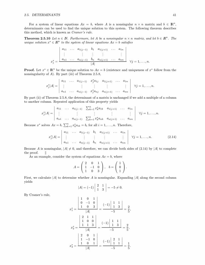
2.5. DETERMINANTS 41
For a system of linear equations Ax = b, where A is a nonsingular n × n matrix and b ∈ IRn,determinants can be used to find the unique solution to this system. The following theorem describesthis method, which is known as Cramer’s rule.
Theorem 2.5.10 Let n ∈ IN. Furthermore, let A be a nonsingular n × n matrix, and let b ∈ IRn. Theunique solution x∗ ∈ IRn to the system of linear equations Ax = b satisfies
x∗j =
∣∣∣∣∣∣∣a11 . . . a1(j−1) b1 a1(j+1) . . . a1n...
......
......
an1 . . . an(j−1) bn an(j+1) . . . ann
∣∣∣∣∣∣∣|A| ∀j = 1, . . . , n.
Proof. Let x∗ ∈ IRn be the unique solution to Ax = b (existence and uniqueness of x∗ follow from thenonsingularity of A). By part (iii) of Theorem 2.5.8,
x∗j |A| =
∣∣∣∣∣∣∣a11 . . . a1(j−1) x
∗ja1j a1(j+1) . . . a1n
......
......
...an1 . . . an(j−1) x
∗janj an(j+1) . . . ann
∣∣∣∣∣∣∣ ∀j = 1, . . . , n.By part (ii) of Theorem 2.5.8, the determinant of a matrix is unchanged if we add a multiple of a columnto another column. Repeated application of this property yields
x∗j |A| =
∣∣∣∣∣∣∣a11 . . . a1(j−1)
∑nk=1 x
∗ka1k a1(j+1) . . . a1n
......
......
...an1 . . . an(j−1)
∑nk=1 x
∗kank an(j+1) . . . ann
∣∣∣∣∣∣∣ ∀j = 1, . . . , n.Because x∗ solves Ax = b,
∑nk=1 x
∗kaik = bi for all i = 1, . . . , n. Therefore,
x∗j |A| =
∣∣∣∣∣∣∣a11 . . . a1(j−1) b1 a1(j+1) . . . a1n...
......
......
an1 . . . an(j−1) bn an(j+1) . . . ann
∣∣∣∣∣∣∣ ∀j = 1, . . . , n. (2.14)
Because A is nonsingular, |A| �= 0, and therefore, we can divide both sides of (2.14) by |A| to completethe proof. ‖As an example, consider the system of equations Ax = b, where
A =
2 0 11 −1 01 0 3
, b =
101
.
First, we calculate |A| to determine whether A is nonsingular. Expanding |A| along the second columnyields
|A| = (−1)∣∣∣∣ 2 11 3
∣∣∣∣ = −5 �= 0.By Cramer’s rule,
x∗1 =
∣∣∣∣∣∣1 0 10 −1 01 0 3
∣∣∣∣∣∣|A| =
(−1)∣∣∣∣ 1 11 3
∣∣∣∣−5 =
2
5,
x∗2 =
∣∣∣∣∣∣2 1 11 0 01 1 3
∣∣∣∣∣∣|A| =
(−1)∣∣∣∣ 1 11 3
∣∣∣∣−5 =
2
5,
x∗3 =
∣∣∣∣∣∣2 0 11 −1 01 0 1
∣∣∣∣∣∣|A| =
(−1)∣∣∣∣ 2 11 1
∣∣∣∣−5 =
1
5.

42 CHAPTER 2. LINEAR ALGEBRA
Determinants can also be used to provide an alternative way of finding the inverse of a nonsingularsquare matrix.
Theorem 2.5.11 Let n ∈ IN. If A is a nonsingular n× n matrix, then
A−1 =1
|A|adj(A).
Proof. By definition, AA−1 = E. Letting a−1ij denote the element in the ith row and jth column of A−1,
we can write this matrix equation as
A
a−11j...a−1nj
= ej ∀j = 1, . . . , n.
By Cramer’s rule,
a−1ij =
∣∣∣∣∣∣∣a11 . . . a1(i−1) e
j1 a1(i+1) . . . a1n
......
......
...an1 . . . an(i−1) e
jn an(i+1) . . . ann
∣∣∣∣∣∣∣|A| ∀i, j = 1, . . . , n.
Expanding along the ith column, we obtain (recall that ejj = 1 and eji = 0 for i �= j)
a−1ij =(−1)i+jAji|A| =
|Cji||A| ∀i, j = 1, . . . , n,
that is,
A−1 =1
|A|adj(A). ‖
2.6 Quadratic Forms
Quadratic forms are expressions in several variables such that each variable appears either as a square orin a product with another variable. Formally, we can write a quadratic form in n variables x1, . . . , xn inthe following way.
Definition 2.6.1 Let n ∈ IN. Furthermore, let αij ∈ IR for all i = 1, . . . , n, j = 1, . . . , i, where αij �= 0for at least one αij. The expression
n∑i=1
i∑j=1
αijxixj
is a quadratic form in the variables x1, . . . , xn.
Every quadratic form in n variables can be expressed as a matrix product
x′Ax
where A is the symmetric n× n matrix given by
A =
α11
12α12 . . . 1
2α1n12α12 α22 . . . 1
2α2n...
......
12α1n
12α2n . . . αnn
. (2.15)
It can be shown that, for given αij, the matrix A defined in (2.15) is the only symmetric n × n matrixsuch that
x′Ax =n∑i=1
i∑j=1
αijxixj.

2.6. QUADRATIC FORMS 43
Therefore, any symmetric square matrix uniquely defines a quadratic form.For example, consider the symmetric matrix
A =
(1 22 −1
).
The quadratic form defined by this matrix is
x′Ax = x21 + 2x1x2 + 2x1x2 − x22 = x21 + 4x1x2 − x22.
The properties of a quadratic form are determined by the properties of the symmetric square ma-trix defining this quadratic form. Of particular importance are the following definiteness properties ofsymmetric square matrices.
Definition 2.6.2 Let n ∈ IN. A symmetric n× n matrix A is
(i) positive definite ⇔ x′Ax > 0 ∀x ∈ IRn \ {0},(ii) negative definite ⇔ x′Ax < 0 ∀x ∈ IRn \ {0},(iii) positive semidefinite ⇔ x′Ax ≥ 0 ∀x ∈ IRn,(iv) negative semidefinite ⇔ x′Ax ≤ 0 ∀x ∈ IRn.
These properties will be of importance later on when we discuss second-order conditions for the opti-mization of functions of several variables.Here are some examples. Let
A =
(2 11 1
), B =
(−2 11 −1
), C =
(1 22 1
).
The quadratic form defined by A is
x′Ax = 2x21 + 2x1x2 + x22 = x
21 + (x1 + x2)
2,
which is positive for all x ∈ IR2 \ {0}. Therefore, A is positive definite. Similarly, we obtain
x′Bx = −2x21 + 2x1x2 − x22 = (−1)(x21 + (x1 − x2)2),
which is negative for all x ∈ IR2 \ {0}, and hence, B is negative definite. Finally, the quadratic formdefined by C is
x′Cx = x21 + 4x1x2 + x22 = 2x1x2 + (x1 + x2)
2.
For x′ = (1, 1), we obtain x′Cx = 6 > 0, and substituting (−1, 1) for x′ yields x′Cx = −2 < 0.Therefore, C is neither positive (semi)definite nor negative (semi)definite. A matrix which is neitherpositive semidefinite nor negative semidefinite is called indefinite.For matrices of higher dimensions, checking definiteness properties can be a quite involved task. There
are some useful criteria for definiteness properties in terms of the determinants of a matrix and some ofits submatrices. Some further definitions are needed in order to introduce these criteria.
Definition 2.6.3 Let n ∈ IN, and let A be an n× n matrix. Furthermore, let k ∈ {1, . . . , n}.
(i) A principal submatrix of order k of A is a k×k matrix that is obtained by removing (n−k)rows and the (n − k) columns with the same numbers from A.(ii) The leading principal submatrix of order k of A is the k × k matrix that is obtained byremoving the last (n−k) rows and columns from A. The leading principal submatrix of orderk of A is denoted by Ak.
For example, the principal submatrices of order 2 of
A =
1 2 00 −1 02 1 −2
are (1 20 −1
),
(1 02 −2
),
(−1 01 −2
).

44 CHAPTER 2. LINEAR ALGEBRA
The leading principal submatrices of orders k = 1, 2, 3 of A are
(1),
(1 20 −1
), A,
respectively. Note that principal submatrices are obtained by removing rows and columns with the samenumbers. For the above matrix A, the submatrix(
1 22 1
)which is obtained by removing row 2 and column 3 from A is not a principal submatrix of A.The determinant of a (leading) principal submatrix is called a (leading) principal minor. Hence, the
leading principal minor of order k of an n× n matrix A is
|Ak| =
∣∣∣∣∣∣∣a11 . . . a1k...
...ak1 . . . akk
∣∣∣∣∣∣∣ .We now can state
Theorem 2.6.4 Let n ∈ IN, and let A be a symmetric n× n matrix. A is(i) positive definite ⇔ |Mk| > 0 for all principal submatrices Mk of order k, for all k =1, . . . , n,(ii) negative definite ⇔ (−1)k|Mk| > 0 for all principal submatrices Mk of order k, for allk = 1, . . . , n,(iii) positive semidefinite ⇔ |Mk| ≥ 0 for all principal submatrices Mk of order k, for allk = 1, . . . , n,(iv) negative semidefinite ⇔ (−1)k|Mk| ≥ 0 for all principal submatrices Mk of order k, forall k = 1, . . . , n.
Proof (for n = 2). Theorem 2.6.4 is true for any n ∈ IN, but we will only prove the case n = 2 here.See more specialized literature for the general proof.(i) “⇒”: By way of contradiction, suppose A is positive definite, but there exists k ∈ {1, 2} and a
principal submatrix Mk of order k such that |Mk| ≤ 0. For n = 2, there are three possible cases.I: a11 ≤ 0;II: a22 ≤ 0;III: |A| ≤ 0.
In case I, let x′ = (1, 0). Then x′Ax = a11 ≤ 0, which contradicts the positive definiteness of A.In case II, let x′ = (0, 1). Then x′Ax = a22 ≤ 0, which again contradicts the positive definiteness of
A.Finally, consider case III. If a22 ≤ 0, we can use the same reasoning as in case II to obtain a contra-
diction. If a22 > 0, let
x1 =√a22, x2 = −
a12√a22.
Then x′Ax = a11a22 − a212 = |A| ≤ 0, contradicting the positive definiteness of A.“⇐”: Suppose a11 > 0, a22 > 0, and |A| = a11a22 − a212 > 0. For any x ∈ IRn \ {0}, we obtain
x′Ax = a11x21 + 2a12x1x2 + a22x
22
= a11x21 + 2a12x1x2 + a22x
22 +a212a11x22 −
a212a11x22
= a11
(x21 + 2
a12
a11x1x2 +
a212a211x22
)+
(a22 −
a212a11
)x22
= a11
(x1 +
a12
a11x2
)2+a11a22 − a212a11
x22
= a11
(x1 +
a12a11x2
)2+|A|a11x22 > 0,

2.6. QUADRATIC FORMS 45
and therefore, A is positive definite.The proof of part (ii) is analogous and left as an exercise.(iii) “⇒”: Suppose A is positive semidefinite, but there exists k ∈ {1, 2} and a principal submatrix
Mk of order k such that |Mk| < 0. Again, there are three possible cases.
I: a11 < 0;II: a22 < 0;III: |A| < 0.
In case I, let x′ = (1, 0). Then x′Ax = a11 < 0, which contradicts the positive semidefiniteness of A.In case II, let x′ = (0, 1). Then x′Ax = a22 < 0, which again contradicts the positive semidefiniteness
of A.Now consider case III. If a22 < 0, we can use the same reasoning as in case II to obtain a contradiction.
If a22 = 0, let x′ = (a12,−(a11 + 1)/2). Then x′Ax = −a212 = |A| < 0, contradicting the positive
semidefiniteness of A. If a22 > 0, let
x1 =√a22, x2 = −
a12√a22.
Again, we obtain x′Ax = a11a22 − a212 = |A| < 0, contradicting the positive semidefiniteness of A.“⇐”: Suppose a11 ≥ 0, a22 ≥ 0, and |A| = a11a22 − a212 ≥ 0. Let x ∈ IRn. If a11 = 0, |A| ≥ 0 implies
a12 = 0, and we obtainx′Ax = a22x
22 ≥ 0.
If a11 > 0, we obtain (analogously to the proof of part (i))
x′Ax = a11
(x1 +
a12
a11x2
)2+|A|a11x22 ≥ 0,
which proves that A is positive semidefinite.The proof of (iv) is analogous and left as an exercise. ‖For positive and negative definiteness, it is sufficient to check the leading principal minors of A.
Theorem 2.6.5 Let n ∈ IN, and let A be a symmetric n× n matrix. A is
(i) positive definite ⇔ |Ak| > 0 ∀k = 1, . . . , n,(ii) negative definite ⇔ (−1)k|Ak| > 0 ∀k = 1, . . . , n.
Proof. Again, we give a proof for n = 2.(i) By Theorem 2.6.4, all that needs to be shown is that the n leading principal minors of A are
positive if and only if all principal minors of order k = 1, . . . , n of A are positive.Clearly, if all principal minors of order k are positive, then, in particular, the leading principal minors
of order k are positive for all k = 1, . . . , n.Conversely, suppose the leading principal minors of A are positive. Therefore, in the case n = 2, we
have a11 > 0 and |A| > 0. Because A is symmetric, |A| > 0 implies a11a22 − a212 > 0. Therefore,
a11a22 > a212. (2.16)
Because a11 > 0, dividing (2.16) by a11 yields a22 > a212/a11 ≥ 0, which completes the proof of (i).
Part (ii) is proven analogously. ‖Therefore, a symmetric n×n matrix A is positive definite if and only if the leading principal minors of
A are positive, and A is negative definite if and only if the signs of the leading principal minors alternate,starting with |A1| = a11 < 0.For positive and negative semidefiniteness, a result analogous to Theorem 2.6.5 can not be obtained.
Checking the leading principal minors is, in general, not sufficient to determine whether a matrix ispositive or negative semidefinite. For example, consider the matrix
A =
(0 00 −1
).

46 CHAPTER 2. LINEAR ALGEBRA
We have |A1| = 0 and |A2| = |A| = 0. Therefore, |Ak| ≥ 0 for all k = 1, 2, but A is not positivesemidefinite, because, for example, choosing x′ = (0, 1) leads to x′Ax = −1 < 0.As an example for the application of Theorems 2.6.4 and 2.6.5, consider again
A =
(2 11 1
), B =
(−2 11 −1
), C =
(1 22 1
).
We obtain |A1| = 2 > 0 and |A2| = |A| = 1 > 0, and therefore, according to Theorem 2.6.5, A is positivedefinite. Furthermore, |B1| = −2 < 0 and |B2| = |B| = 1 > 0, which means that B is negative definite.Finally, |C1| = 1 > 0 and |C2| = |C| = −3 < 0. According to Theorem 2.6.4, C is neither positivesemidefinite nor negative semidefinite, and therefore, C is indefinite.

Chapter 3
Functions of One Variable
3.1 Continuity
In this chapter, we discuss functions the domain and range of which are subsets of IR. Hence, a real-valuedfunction of one variable is a function f : A �→ B where A ⊆ IR and B ⊆ IR. To simplify matters, weassume that A is an interval of the form [a, b] with a, b ∈ IR or (a, b) with a ∈ IR ∪ {−∞}, b ∈ IR ∪ {∞}or [a, b) with a ∈ IR, b ∈ IR ∪ {∞} or (a, b] with a ∈ IR ∪ {−∞}, b ∈ IR, where a < b. It should be notedthat some, but not all, of the results stated in this chapter can be generalized to domains that are notnecessarily intervals. The range of f will, in most cases, simply be the set IR itself.In many economic models (and in other applications), real-valued functions are assumed to be con-
tinuous. Loosely speaking, continuity ensures that “small” changes in the argument of a function do notlead to “large” changes in the value of the function. The formal definition of continuity is
Definition 3.1.1 Let A ⊆ IR, and let f : A �→ IR be a function. Furthermore, let x0 ∈ A.(i) The function f is continuous at x0 if and only if
∀δ ∈ IR++, ∃ε ∈ IR++ such that f(x) ∈ Uδ(f(x0)) ∀x ∈ Uε(x0) ∩A.
(ii) The function f is continuous on A0 ⊆ A if and only if f is continuous at each x0 ∈ A0. If f iscontinuous on A, we will often simply say that f is continuous.
According to this definition, a function f is continuous at a point x0 in its domain if, for each neighborhoodof f(x0), there exists a neighborhood of x0 such that f(x) is in this neighborhood of f(x0) for all x inthe domain of f that are in the neighborhood of x0.Consider the following example. Let
f : IR �→ IR, x �→ 2x,
and let x0 = 1. Then f(x0) = f(1) = 2. To show that the function f is continuous at x0 = 1, we have toshow that, for any δ ∈ IR++, we can find an ε ∈ IR++ such that
f(x) ∈ (2− δ, 2 + δ) ∀x ∈ (1− ε, 1 + ε).
For δ ∈ IR++, let ε := δ/2. Then, for all x ∈ Uε(1) = (1− δ/2, 1 + δ/2),
f(x) > 2(1− ε) = 2(1− δ/2) = 2− δ and f(x) < 2(1 + ε) = 2(1 + δ/2) = 2 + δ.
Therefore, f(x) ∈ Uδ(2) for all x ∈ Uε(1). Similarly, it can be shown that f is continuous at any pointx0 ∈ IR (Exercise: provide a proof), and therefore, f is continuous on its domain IR.As another example, consider the function
f : IR �→ IR, x �→{0 if x ≤ 01 if x > 0.
This function is not continuous at x0 = 0. To show this, let δ = 1/2. Continuity of f at x0 = 0 requiresthat there exists ε ∈ IR++ such that f(x) ∈ (−1/2, 1/2) for all x ∈ Uε(0) = (−ε, ε). For any ε ∈ IR++,
47

48 CHAPTER 3. FUNCTIONS OF ONE VARIABLE
x
f(x)
x0
f(x0)
f(x0)− δ
f(x0) + δ
x0 − ε x0 + ε
Figure 3.1: A continuous function.
x
f(x)
x0
f(x0)
f(x0)− δ
f(x0) + δ u
Figure 3.2: A discontinuous function.
Uε(0) contains points x > 0, and therefore, any neighborhood of x0 = 0 contains points x such thatf(x) = 1 �∈ Uδ(f(x0)) = (−1/2, 1/2). Therefore, f is not continuous at x0 = 0.Using the graph of a function, continuity can be illustrated in a diagram. Figure 3.1 gives an example
of the graph of a function f that is continuous at x0, whereas the function with the graph illustrated inFigure 3.2 is not continuous at the point x0.
An alternative definition of continuity can be given in terms of sequences of real numbers.
Theorem 3.1.2 Let A ⊆ IR be an interval, and let f : A �→ IR be a function. Furthermore, let x0 ∈ A.f is continuous at x0 if and only if, for all sequences {xn} such that xn ∈ A for all n ∈ IN,
limn→∞
xn = x0⇒ limn→∞
f(xn) = f(x0).
Proof. “Only if”: Suppose f is continuous at x0 ∈ A. Then, for any δ ∈ IR++, there exists ε ∈ IR++such that
f(x) ∈ Uδ(f(x0)) ∀x ∈ Uε(x0) ∩A.

3.1. CONTINUITY 49
Let {xn} be a sequence such that xn ∈ A for all n ∈ IN and {xn} converges to x0. Because limn→∞ xn =x0, we can find n0 ∈ IN such that
|xn − x0| < ε ∀n ≥ n0.
Therefore, |f(xn)− f(x0)| < δ for all n ≥ n0, which implies that {f(xn)} converges to f(x0).“If”: Suppose f is not continuous at x0 ∈ A. Then there exists δ ∈ IR++ such that, for all ε ∈ IR++,
there exists x ∈ Uε(x0) ∩A withf(x) �∈ Uδ(f(x0)).
Let εn := 2/n for all n ∈ IN. By assumption, for any n ∈ IN, there exists xn ∈ Uεn(x0) ∩A such that
|f(xn) − f(x0)| ≥ δ. (3.1)
Because xn ∈ Uεn(x0) ∩A for all n ∈ IN, the sequence {xn} converges to x0. By (3.1), {f(xn)} does notconverge to f(x0), which completes the proof. ‖Theorem 3.1.2 is particularly useful in proving that a function is not continuous at a point x0 in its
domain. One only has to find one sequence {xn} that converges to x0 such that the sequence {f(xn)}does not converge to f(x0).We now introduce limits of a function which are closely related to limits of sequences.
Definition 3.1.3 Let A ⊆ IR, and let f : A �→ IR be a function. Furthermore, let α ∈ IR ∪ {−∞,∞}.(i) Let x0 ∈ IR ∪ {−∞}, and suppose (x0, x0 + h) ⊆ A for some h ∈ IR++. The right-side limit of
f at x0 exists and is equal to α if and only if, for all monotone nonincreasing sequences {xn} such thatxn ∈ A for all n ∈ IN,
xn −→ x0 ⇒ f(xn) −→ α.
If the right-side limit of f at x0 exists and is equal to α, we write limx↓x0 f(x) = α.
(ii) Let x0 ∈ IR∪{∞}, and suppose (x0−h, x0) ⊆ A for some h ∈ IR++. The left-side limit of f at x0exists and is equal to α if and only if, for all monotone nondecreasing sequences {xn} such that xn ∈ Afor all n ∈ IN,
xn −→ x0 ⇒ f(xn) −→ α.
If the left-side limit of f at x0 exists and is equal to α, we write limx↑x0 f(x) = α.
(iii) Let x0 ∈ IR, and suppose (x0−h, x0)∪ (x0, x0+ h) ⊆ A for some h ∈ IR++. The limit of f at x0exists and is equal to α if and only if the right-side and left-side limits of f at x0 exist and are equal toα. If the limit of f at x0 exists and is equal to α, we write limx→x0 f(x) = α.
For finite values of x0 and α, an equivalent definition of a limit can be given directly (that is, withoutusing sequences). We obtain
Theorem 3.1.4 Let A ⊆ IR, and let f : A �→ IR be a function. Furthermore, let x0 ∈ IR, α ∈ IR, andsuppose (x0 − h, x0) ∪ (x0, x0 + h) ⊆ A for some h ∈ IR++. The limit of f at x0 exists and is equal to αif and only if
∀δ ∈ IR++, ∃ε ∈ IR++ such that f(x) ∈ Uδ(α) ∀x ∈ Uε(x0).
Analogous results are valid for one-sided limits.For interior points of the domain of a function, continuity at these points can be formulated in terms
of limits. We obtain
Theorem 3.1.5 Let A ⊆ IR be an interval, and let f : A �→ IR be a function. Furthermore, let x0 be aninterior point of A. f is continuous at x0 if and only if limx→x0 f(x) exists and limx→x0 f(x) = f(x0).
Theorem 3.1.5 can be proven by combining Theorem 3.1.2 and Definition 3.1.3.Analogously, for boundary points of A, we obtain
Theorem 3.1.6 Let A = [a, b] with a, b ∈ IR and a < b. Furthermore, let f : A �→ IR be a function.
(i) f is continuous at a if and only if limx↓a f(x) exists and limx↓a f(x) = f(a).(ii) f is continuous at b if and only if limx↑b f(x) exists and limx↑b f(x) = f(b).

50 CHAPTER 3. FUNCTIONS OF ONE VARIABLE
To illustrate the application of Theorem 3.1.5, consider the following examples. Let
f : IR �→ IR, x �→ 2x.
We use Theorem 3.1.5 to prove that f is continuous at x0 = 1. We obtain
limx↑1f(x) = lim
x↑12x = 2
andlimx↓1f(x) = lim
x↓12x = 2,
and therefore, limx→1 f(x) exists and is equal to 2. Furthermore, f(1) = 2, and therefore, according toTheorem 3.1.5, f is continuous at x0 = 1.Now let
f : IR �→ IR, x �→{0 if x ≤ 01 if x > 0.
Let x0 = 0. We havelimx↑0f(x) = lim
x↑00 = 0
andlimx↓0f(x) = lim
x↓01 = 1,
and therefore, limx→0 f(x) does not exist. By Theorem 3.1.5, f is not continuous at x0 = 0.Finally, consider the function given by
f : IR �→ IR, x �→{0 if x = 01 if x �= 0.
For x0 = 0, we obtainlimx↑0f(x) = lim
x↑01 = 1
andlimx↓0f(x) = lim
x↓01 = 1.
Therefore, limx→0 f(x) exists and is equal to 1. But we have f(0) = 0 �= 1, and hence, f is not continuousat x0 = 0.The following definition introduces some notation for functions that can be defined using other func-
tions.
Definition 3.1.7 Let A ⊆ IR be an interval, and let f : A �→ IR and g : A �→ IR be functions. Further-more, let α ∈ IR.(i) The sum of f and g is the function defined by
f + g : A �→ IR, x �→ f(x) + g(x).
(ii) The function αf is defined by
αf : A �→ IR, x �→ αf(x).
(iii) The product of f and g is the function defined by
fg : A �→ IR, x �→ f(x)g(x).
(iv) If g(x) �= 0 for all x ∈ A, the ratio of f and g is the function defined by
f
g: A �→ IR, x �→ f(x)
g(x).
Some useful results concerning the continuity of functions are summarized in

3.1. CONTINUITY 51
Theorem 3.1.8 Let A ⊆ IR be an interval, and let f : A �→ IR and g : A �→ IR be functions. Furthermore,let α ∈ IR. If f and g are continuous at x0 ∈ A, then
(i) f + g is continuous at x0.(ii) αf is continuous at x0.(iii) fg is continuous at x0.(iv) If g(x) �= 0 for all x ∈ A, f/g is continuous at x0.
The proof of this theorem follows from the corresponding properties of sequences and Theorem 3.1.2.Furthermore, if two functions f : A �→ IR and g : f(A) �→ IR are continuous, then the composite
function g ◦ f is continuous. We state this result without a proof.Theorem 3.1.9 Let A ⊆ IR be an interval. Furthermore, let f : A �→ IR and g : f(A) �→ IR be functions,and let x0 ∈ A. If f is continuous at x0 and g is continuous at y0 = f(x0), then g ◦ f is continuous atx0.
If the domain of a continuous function is an interval, the inverse of this function is continuous.
Theorem 3.1.10 Let A ⊆ IR be an interval, let B ⊆ IR, and let f : A �→ B be bijective. If f is continuouson A, then f−1 is continuous on B = f(A).
The assumption that A is an interval is essential in this theorem. For some bijective functions f withmore general domains A ⊆ IR, continuity of f does not imply continuity of f−1. To illustrate that,consider the following example. Let
f : [0, 1] ∪ (2, 3] �→ [0, 2], x �→{
x2 if x ∈ [0, 1]x− 1 if x ∈ (2, 3].
The domain of this function is A = [0, 1] ∪ (2, 3], which is not an interval. The function f is continuouson A and bijective (Exercise: show this). The inverse of f exists and is given by
f−1 : [0, 2] �→ [0, 1]∪ (2, 3], y �→{ √
y if y ∈ [0, 1]y + 1 if y ∈ (1, 2].
Clearly, f−1 is not continuous at y0 = 1.Some important examples for continuous functions are polynomials.
Definition 3.1.11 Let A ⊆ IR be an interval, and let f : A �→ IR be a function. Furthermore, letn ∈ IN ∪ {0}. f is a polynomial of degree n if and only if there exist α0, . . . , αn ∈ IR with αn �= 0 ifn ∈ IN such that
f(x) =n∑i=0
αixi ∀x ∈ A.
For example, the functionf : IR �→ IR, x �→ −2 + x− 2x3
is a polynomial of degree three. Other examples for polynomials are constant functions, defined by
f : IR �→ IR, x �→ α
where α ∈ IR is a constant, affine functions
f : IR �→ IR, x �→ α+ βx
where α, β ∈ IR, β �= 0, and quadratic functions
f : IR �→ IR, x �→ α+ βx + γx2
where α, β, γ ∈ IR, γ �= 0. Constant functions are polynomials of degree zero, affine functions arepolynomials of degree one, and quadratic functions are polynomials of degree two.Because the function
f : IR �→ IR, x �→ xn
is continuous for any n ∈ IN (Exercise: prove this), Theorem 3.1.8 implies that all polynomials arecontinuous.Analogously to monotonic sequences, monotonicity properties of functions can be defined. We con-
clude this section with the definitions of these properties.

52 CHAPTER 3. FUNCTIONS OF ONE VARIABLE
x
f(x)
x0
f(x0)
x0 + h
f(x0 + h)
x0 + h
f(x0 + h)
Figure 3.3: The difference quotient.
Definition 3.1.12 Let A ⊆ IR be an interval, and let B ⊆ A. Furthermore, let f : A �→ IR be a function.(i) f is (monotone) nondecreasing on B if and only if
x > y ⇒ f(x) ≥ f(y) ∀x, y ∈ B.
(ii) f is (monotone) increasing on B if and only if
x > y ⇒ f(x) > f(y) ∀x, y ∈ B.
(iii) f is (monotone) nonincreasing on B if and only if
x > y ⇒ f(x) ≤ f(y) ∀x, y ∈ B.
(iv) f is (monotone) decreasing on B if and only if
x > y ⇒ f(x) < f(y) ∀x, y ∈ B.
If f is nondecreasing (respectively increasing, nonincreasing, decreasing) on its domain A, we will some-times simply say that f is nondecreasing (respectively increasing, nonincreasing, decreasing).
3.2 Differentiation
An important issue concerning real-valued functions of one real variable is the question how the value of afunction changes as a consequence of a change in its argument. We first give a diagrammatic illustration.Consider the graph of a function f : IR �→ IR as illustrated in Figure 3.3.Suppose we want to find the rate of change in the value of f as a consequence of a change in the
variable x from x0 to x0+h. A natural way to do this is to use the slope of the secant through the points(x0, f(x0)) and (x0 + h, f(x0 + h)). Clearly, this slope is given by the ratio
f(x0 + h)− f(x0)h
. (3.2)
The quotient in (3.2) is called the difference quotient of f for x0 and h. This slope depends on thenumber h ∈ IR we add to x0 (h can be positive or negative). Depending on f , the values of the differencequotient for given x0 can differ substantially for different values of h—consider, for example, the differencequotients that are obtained with h and with h in Figure 3.3.

3.2. DIFFERENTIATION 53
In order to obtain some information about the behaviour of f “close” to a point x0, it is desirableto find an indicator that is independent of the number h which represents the deviation from x0. Thenatural way to proceed is to use the limit of the difference quotient as h approaches zero as an indicatorof the change in f at x0. If this limit exists and is finite, we say that the function is differentiable at thepoint x0. Formally,
Definition 3.2.1 Let A ⊆ IR, and let f : A �→ IR be a function. Furthermore, let x0 be an interior pointof A. The function f is differentiable at x0 if and only if
limh→0
f(x0 + h) − f(x0)h
(3.3)
exists and is finite. If f is differentiable at x0, we call the limit in (3.3) the derivative of f at x0 anddenote it by f ′(x0).
Definition 3.2.1 applies to interior points of A only. We can also define “one-sided” derivatives at theendpoints of the interval A, if these points are elements of A.
Definition 3.2.2 Let f : [a, b] �→ IR with a, b ∈ IR and a < b.(i) f is (right-side) differentiable at a if and only if
limh↓0
f(a + h)− f(a)h
(3.4)
exists and is finite. If f is (right-side) differentiable at a, we call the limit in (3.4) the (right-side)derivative of f at a and denote it by f ′(a).
(ii) f is (left-side) differentiable at b if and only if
limh↑0
f(b + h)− f(b)h
(3.5)
exists and is finite. If f is (left-side) differentiable at b, we call the limit in (3.5) the (left-side) derivativeof f at b and denote it by f ′(b).
A function f : A �→ IR is differentiable on an interval B ⊆ A if f ′(x0) exists for all interior points x0 ofB, and the right-side and left-side derivatives of f at the endpoints of B exist whenever these endpointsbelong to B. If f : A �→ IR is differentiable on A, the function
f ′ : A �→ IR, x �→ f ′(x)
is called the derivative of f . If the function f ′ is differentiable at x0 ∈ A, we can find the second derivativeof f at x0, which is just the derivative of f
′ at x0. Formally, if f′ : A �→ IR is differentiable at x0 ∈ A, we
call
f ′′(x0) = limh→0
f ′(x0 + h)− f ′(x0)h
the second derivative of f at x0. Analogously, we can define higher-order derivatives of f , and we writef(n)(x0) for the n
th derivative of f at x0 (where n ∈ IN), if this derivative exists.For a function f which is differentiable at a point x0 in its domain, f
′(x0) is the slope of the tangentto the graph of f at x0. The equation of this tangent for a differentiable function f : A �→ IR at x0 ∈ A is
y = f(x0) + f′(x0)(x− x0) ∀x ∈ A.
As an example, consider the following function
f : IR �→ IR, x �→ 2 + x+ 4x2.
To determine whether or not this function is differentiable at a point x0 in its domain, we have to findout whether the limit of the difference quotient as h approaches zero exists and is finite. For the above

54 CHAPTER 3. FUNCTIONS OF ONE VARIABLE
function f and x0 ∈ IR, we obtain
f(x0 + h)− f(x0)h
=2 + x0 + h+ 4(x0 + h)
2 − 2− x0 − 4(x0)2h
=h+ 4((x0)
2 + 2x0h+ h2)− 4(x0)2
h
=h+ 8x0h+ 4h
2
h= 1 + 8x0 + 4h.
Clearly,limh→0(1 + 8x0 + 4h) = 1 + 8x0,
and therefore, f is differentiable at any point x0 ∈ IR with f ′(x0) = 1 + 8x0.Differentiability is a stronger requirement than continuity. This is shown in the following theorems.
Theorem 3.2.3 Let A ⊆ IR be an interval, and let f : A �→ IR be a function. Furthermore, let x0 be aninterior point of A. If f is differentiable at x0, then f is continuous at x0.
Proof. For h ∈ IR such that (x0 + h) ∈ A and h �= 0, we obtain
f(x0 + h) − f(x0) =(f(x0 + h)− f(x0)
h
)h.
Because f is differentiable at x0,
limh→0(f(x0 + h)− f(x0)) = f ′(x0) lim
h→0h = 0.
This implieslimh→0f(x0 + h) = f(x0).
Defining x := x0 + h, this can be written as
limx→x0
f(x) = f(x0),
which proves that f is continuous at x0. ‖Again, we can extend the result of Theorem 3.2.3 to boundary points of A.
Theorem 3.2.4 Let f : [a, b] �→ IR with a, b ∈ IR and a < b.
(i) If f is right-side differentiable at a, then f is continuous at a.(ii) If f is left-side differentiable at b, then f is continuous at b.
The proof of this theorem is analogous to the proof of Theorem 3.2.3 and is left as an exercise.Continuity does not imply differentiability. Consider, for example, the function
f : IR �→ IR, x �→ |x|.
This function is continuous at x0 = 0, but it is not differentiable at x0 = 0. To show this, note that
limx↓0f(x) = lim
x↓0x = 0, lim
x↑0f(x) = lim
x↑0−x = 0,
and f(0) = 0. Therefore, limx→0 f(x) exists and is equal to f(0) = 0, which shows that f is continuousat x0 = 0.Now note that
limh↓0
f(0 + h)− f(0)h
=h
h= 1
and
limh↑0
f(0 + h) − f(0)h
=−hh= −1.

3.2. DIFFERENTIATION 55
Clearly,
limh↓0
f(0 + h)− f(0)h
�= limh↑0
f(0 + h)− f(0)h
,
and therefore,
limh→0
f(0 + h)− f(0)h
does not exist, which implies that f is not differentiable at x0 = 0.The following theorem introduces some rules of differentiation which simplify the task of finding the
derivatives of certain differentiable functions. It states that sums, multiples, products, and ratios ofdifferentiable functions are differentiable, and shows how these derivatives are obtained.
Theorem 3.2.5 Let A ⊆ IR be an interval, and let f : A �→ IR, g : A �→ IR be functions. Furthermore,let α ∈ IR. Let x0 be an interior point of A, and suppose f and g are differentiable at x0.(i) f + g is differentiable at x0, and (f + g)
′(x0) = f′(x0) + g
′(x0).(ii) αf is differentiable at x0, and (αf)
′(x0) = αf′(x0).
(iii) fg is differentiable at x0, and (fg)′(x0) = f
′(x0)g(x0) + f(x0)g′(x0).
(iv) If g(x0) �= 0, then f/g is differentiable at x0, and(f
g
)′(x0) =
f ′(x0)g(x0)− f(x0)g′(x0)[g(x0)]2
.
Proof. (i) Because f and g are differentiable at x0, f′(x0) and g
′(x0) exist. Now it follows that
limh→0
f(x0 + h) + g(x0 + h)− f(x0)− g(x0)h
= limh→0
f(x0 + h)− f(x0)h
+ limh→0
g(x0 + h)− g(x0)h
= f ′(x0) + g′(x0).
(ii) limh→0
αf(x0 + h)− αf(x0)h
= α limh→0
f(x0 + h)− f(x0)h
= αf ′(x0).
(iii) limh→0
f(x0 + h)g(x0 + h)− f(x0)g(x0)h
= limh→0
f(x0 + h)g(x0 + h)− f(x0)g(x0 + h)h
+ limh→0
f(x0)g(x0 + h)− f(x0)g(x0)h
= limh→0
f(x0 + h)− f(x0)h
g(x0 + h)
+ limh→0f(x0)
g(x0 + h)− g(x0)h
= f ′(x0)g(x0) + f(x0)g′(x0).
(iv) Because g is differentiable at x0, g is continuous at x0. Therefore, g(x0) �= 0 implies that thereexists a neighborhood of x0 such that g(x) �= 0 for all x ∈ A in this neighborhood. Let h ∈ IR be suchthat (x0 + h) is in this neighborhood. Then we obtain
limh→0
f(x0 + h)/g(x0 + h) − f(x0)/g(x0)h
= limh→0
f(x0 + h)g(x0) − f(x0)g(x0 + h)hg(x0 + h)g(x0)
=
limh→0
g(x0)[f(x0 + h)− f(x0)]− f(x0)[g(x0 + h)− g(x0)]hg(x0 + h)g(x0)
=f ′(x0)g(x0) − f(x0)g′(x0)
[g(x0)]2. ‖
Replacing the limits in the above proof by the corresponding one-sided limits, we obtain analogous resultsfor boundary points of A. The formulation of these results is left as an exercise.We now find the derivatives of some important functions. First, consider affine functions of the form
f : IR �→ IR, x �→ α+ βx

56 CHAPTER 3. FUNCTIONS OF ONE VARIABLE
with α, β ∈ IR and β �= 0. Let x ∈ IR. Then
limh→0
f(x + h)− f(x)h
= limh→0
α+ β(x + h) − α− βxh
= limh→0
βh
h= β.
Therefore, f ′(x) = β for all x ∈ IR.Now consider the linear function
f : IR �→ IR, x �→ βxwith β ∈ IR, β �= 0. For any x ∈ IR, we obtain
limh→0
f(x + h) − f(x)h
= limh→0
β(x + h) − βxh
= limh→0β = β,
and therefore, f ′(x) = β for all x ∈ IR.If f is a constant function
f : IR �→ IR, x �→ αwith α ∈ IR, we can write f as
f : IR �→ IR, x �→ α+ βx − βxwith β ∈ IR, β �= 0. Parts (i) and (ii) of Theorem 3.2.5 imply, together with the above results for affineand linear functions,
f ′(x) = 0 ∀x ∈ IR. (3.6)
Next, letf : IR �→ IR, x �→ xn
where n ∈ IN. For x ∈ IR, we obtain the difference quotientf(x + h) − f(x)
h=(x+ h)n − xn
h.
The binomial formula (which we will not prove here) says that, for x, y ∈ IR and n ∈ IN,
(x + y)n =n∑k=0
n!
k!(n− k)!xn−kyk.
Therefore, we obtain
limh→0
f(x + h) − f(x)h
= limh→0
∑nk=0
n!k!(n−k)!x
n−khk − xn
h
= limh→0
∑nk=1
n!k!(n−k)!x
n−khk
h
= limh→0
nxn−1h+∑nk=2
n!k!(n−k)!x
n−khk
h
= nxn−1 + limh→0
n∑k=2
n!
k!(n− k)!xn−khk−1
= nxn−1.
Therefore,f ′(x) = nxn−1 ∀x ∈ IR. (3.7)
If we have a polynomial
f : IR �→ IR, x �→n∑i=0
αixi
with n ∈ IN, Theorem 3.2.5, (3.6), and (3.7) can be applied to conclude
f ′(x) =n∑i=1
iαixi−1 ∀x ∈ IR.
A very useful rule for differentiation that applies to composite functions is the chain rule, which isdescribed in the following theorem.

3.2. DIFFERENTIATION 57
Theorem 3.2.6 Let A ⊆ IR be an interval, and let f : A �→ IR, g : f(A) �→ IR be functions. Let x0 bean interior point of A. If f is differentiable at x0 and g is differentiable at y0 = f(x0), then g ◦ f isdifferentiable at x0, and
(g ◦ f)′(x0) = g′(f(x0))f ′(x0).
Proof. Let y0 = f(x0). For r ∈ IR such that (y0 + r) ∈ f(A), define
k(y0 + r) :=
{g(y0+r)−g(y0)
rif r �= 0
g′(y0) if r = 0.
Because g is differentiable at y0,limr→0k(y0 + r) = g
′(y0).
Furthermore, by definition,g(y0 + r)− g(y0) = rk(y0 + r).
Therefore, for h ∈ IR \ {0} such that (x0 + h) ∈ A,
g(f(x0 + h))− g(f(x0)) = [f(x0 + h)− f(x0)]k(f(x0 + h)),
and hence,g(f(x0 + h))− g(f(x0))
h=f(x0 + h)− f(x0)
hk(f(x0 + h)).
Taking limits, we obtain
(g ◦ f)′(x0) = limh→0
g(f(x0 + h))− g(f(x0))h
= limh→0
f(x0 + h)− f(x0)h
k(f(x0 + h))
= g′(f(x0))f′(x0). ‖
Again, it is straightforward to obtain analogous theorems for boundary points of A by considering one-sided limits.As an example for the application of the chain rule, let
f : IR �→ IR, x �→ 2x− 3x2
andg : IR �→ IR, y �→ y3.
Theng ◦ f : IR �→ IR, x �→ (2x− 3x2)3.
We obtainf ′(x) = 2− 6x ∀x ∈ IR
andg′(y) = 3y2 ∀y ∈ IR.
According to the chain rule,
(g ◦ f)′(x) = g′(f(x))f ′(x) = 3(2x− 3x2)2(2− 6x) ∀x ∈ IR.
The following theorem (which we state without a proof) provides a relationship between the derivativeof a bijective function and its inverse.
Theorem 3.2.7 Let A,B ⊆ IR, where A = (a, b) with a, b ∈ IR, a < b. Furthermore, let f : A �→ B bebijective and continuous. If f is differentiable at x0 ∈ A = (a, b) and f ′(x0) �= 0, then f−1 is differentiableat y0 = f(x0), and
(f−1)′(y0) =1
f ′(x0).

58 CHAPTER 3. FUNCTIONS OF ONE VARIABLE
To conclude this section, we introduce some important functions and their properties. First, we definethe exponential function.
Definition 3.2.8 The function
E : IR �→ IR++, x �→∞∑n=0
xn
n!
is called the exponential function.
The definition of E involves an infinite sum, but it can be shown that this sum converges for all x ∈ IR,and therefore, E is a well-defined function. Another (equivalent) definition of E is given by the followingtheorem, which is stated without a proof.
Theorem 3.2.9 For all x ∈ IR,E(x) = lim
n→∞
(1 +x
n
)n.
The exponential function is used, for example, to describe certain growth processes. Before discussingan application, we introduce some important properties of E and related functions. We only prove part(i) of the following theorem.
Theorem 3.2.10 (i) The function E is differentiable on IR, and E′(x) = E(x) ∀x ∈ IR.(ii) E is increasing, limx↑∞E(x) =∞, limx↓−∞E(x) = 0, and E(IR) = IR++.(iii) E(0) = 1.(iv) E(1) = e = 2.71828 . . ..(v) E(x+ y) = E(x)E(y) ∀x, y ∈ IR.
Proof of (i). For x ∈ IR, we obtain (using the rules of differentiation for polynomials)
E′(x) =∞∑n=1
nxn−1
n!=
∞∑n=1
xn−1
(n− 1)! =∞∑m=0
xm
m!= E(x). ‖
Part (i) of this theorem is quite remarkable. It states that for any x ∈ IR, the derivative of E at x isequal to the value of E at x.Parts (iv) and (v) of Theorem 3.2.10 imply
E(2) = E(1 + 1) = E(1)E(1) = e2,
and, in general, for n ∈ IN,E(n) = en.
Furthermore, we obtain
E(−n) = 1
E(n)= e−n ∀n ∈ IN.
Now let y ∈ IR. For a rational number x = p/q with p ∈ Z and q ∈ IN, we obtain
(E(xy))q = E(qxy) = E(py) = (E(y))p ,
and therefore,E(xy) = q
√(E(y))p = (E(y))p/q = (E(y))x.
For y = 1, this impliesE(x) = (E(1))x = ex ∀x ∈ Q.
More generally, we can defineex := E(x) ∀x ∈ IR,
that is, ex is defined by E(x), even if x is an irrational number.The graph of the exponential function can be illustrated as in Figure 3.4.Part (ii) of Theorem 3.2.10 implies that E is bijective, and therefore, E has an inverse. We call the
inverse of the exponential function the natural logarithm.

3.2. DIFFERENTIATION 59
-2 -1 0 1 2 x
1
2
3
4
5
E(x)
e
Figure 3.4: The exponential function.
Definition 3.2.11 The natural logarithm ln : IR++ �→ IR is defined as the inverse function of theexponential function, that is, ln = E−1.
By definition of an inverse, we have
E(ln(x)) = eln(x) = x ∀x ∈ IR++
andln(E(x)) = ln(ex) = x ∀x ∈ IR.
From the properties of E, it follows that ln must have certain properties. Some of them are summarizedin the following theorem.
Theorem 3.2.12 (i) The function ln is differentiable on IR++, and ln′(x) = 1/x ∀x ∈ IR++.
(ii) ln is increasing, limx↑∞ ln(x) =∞, limx↓0 ln(x) = −∞, and ln(IR++) = IR.(iii) ln(1) = 0.(iv) ln(e) = 1.(v) ln(xy) = ln(x) + ln(y) ∀x, y ∈ IR++.
The natural logarithm can also be written as an infinite sum, namely,
ln(x) =∞∑n=1
(−1)n−1n
(x− 1)n ∀x ∈ IR++.
An important implication of part (v) of Theorem 3.2.12 is
ln(xn) = n ln(x) ∀x ∈ IR++, ∀n ∈ IN.
Because ln = E−1, we obtain
xn = E(ln(xn)) = E(n ln(x)) ∀x ∈ IR++, ∀n ∈ IN.
Therefore, the power function xn can be expressed in terms of exponential and logarithmic functions.More generally, we can define generalized powers in the following way. For x ∈ IR++ and y ∈ IR, we define
xy := E(y ln(x)).
This allows us to define generalizations of power functions such as
f : IR++ �→ IR, x �→ xα

60 CHAPTER 3. FUNCTIONS OF ONE VARIABLE
where α ∈ IR (note that α is not restricted to natural or rational numbers). Functions of this type arecalled generalized power functions. Similarly, we can define functions such as
f : IR �→ IR++, x �→ αx
where α ∈ IR++. Note that the variable x appears in the exponent. These functions are called generalizedexponential functions. Clearly, a special case is the function E, which is obtained by setting α = e.Using the properties of E and ln, it is now easy to find the derivatives of generalized power functions
and generalized exponential functions. Let
f : IR++ �→ IR, x �→ xα
with α ∈ IR. By definition,f(x) = E(α ln(x)) ∀x ∈ IR++.
Using the chain rule, we obtain, for x ∈ IR++,
f ′(x) = E′(α ln(x))α1
x= E(α ln(x))α
1
x= xαα
1
x= αxα−1,
and therefore, the differentiation rule for power functions generalizes naturally.For the function
f : IR �→ IR++, x �→ αx
with α ∈ IR++, we havef(x) = E(x ln(α)) ∀x ∈ IR.
Applying the chain rule, it follows that
f ′(x) = E′(x ln(α)) ln(α) = E(x ln(α)) ln(α) = αx ln(α)
for all x ∈ IR.The inverse of a generalized exponential function is a logarithmic function, which generalizes the
natural logarithm.
Definition 3.2.13 Let α ∈ IR++ \ {1}, and let Eα : IR �→ IR++ be a generalized exponential function.The logarithm to the base α, logα : IR++ �→ IR, is the inverse of Eα, that is, logα = E−1α .
By definition of the generalized exponential functions, we obtain, for all x ∈ IR++,
x = E(ln(x)) = Eα(logα(x)) = αlogα(x) = E(logα(x) ln(α)).
Taking logarithms on both sides, we obtain
ln(x) = ln(E(logα(x) ln(α))) = logα(x) ln(α),
and therefore,
logα(x) =ln(x)
ln(α)∀x ∈ IR++.
Therefore, the logarithm to any base α ∈ IR++ \ {1} can be expressed in terms of the natural logarithm.As was mentioned earlier, exponential functions play an important role in growth models. Suppose,
for example, the real national income in an economy is described by a function
Y : IN ∪ {0} �→ IR++, t �→ Y (t)
where t is a variable that represents time, and hence, Y (t) is the national income in period t = 0, 1, 2, . . ..A standard formulation of a model describing economic growth is to use functions involving exponentialgrowth. For example, define
Y : IN ∪ {0} �→ IR++, t �→ y0(1 + r)t
where y0 ∈ IR++, and r ∈ IR++ is the growth rate. By setting t = 0, we see that y0 = Y (0), that is, y0 isthe initial value for the growth process described by Y .

3.2. DIFFERENTIATION 61
In discussing economic growth, one should keep in mind that exponential growth (that is, growthinvolving a growth rate at or above a given positive rate) cannot be expected to be sustainable in thelong run. Consider the following example. Suppose the annual growth rate is 5%. How long will it take,given this growth rate, to double the initial national income? To answer this question, we have to findt ∈ IN such that
Y (t) ≥ 2Y (0). (3.8)
For an exponential growth process with r = 0.05, we obtain
Y (t) = Y (0)(1.05)t,
and therefore, (3.8) is equivalent to
(1.05)t ≥ 2.
Taking logarithms on both sides, we obtain
t ln(1.05) ≥ ln(2),
or
t ≥ ln(2)
ln(1.05)= 14.2067.
Therefore, if a growth process is described by an exponential function with a growth rate of 5%, it takesonly 14 years to double the existing national income. If no further assumptions on how and in whichsectors this growth comes about are made, this clearly could lead to rather undesirable results (such asirreparable environmental damage), and therefore, the growth rate of real national income alone is not auseful indicator for the societal well-being in an economy.We conclude this section with a discussion of the two basic trigonometric functions.
Definition 3.2.14 The function
sin : IR �→ IR, x �→∞∑n=0
(−1)n x2n+1
(2n+ 1)!
is called the sine function.
Definition 3.2.15 The function
cos : IR �→ IR, x �→∞∑n=0
(−1)n x2n
(2n)!
is called the cosine function.
A geometric interpretation of those two functions is provided in Figure 3.5. Consider a circle aroundthe origin of IR2 with radius r = 1. Starting at the point (1, 0), let x be the distance travelled counter-clockwise along the circle. The first coordinate of the resulting point is the value of the cosine functionat x and its second coordinate is the value of the sine function at x.The following theorem states some important properties of the sine and cosine functions.
Theorem 3.2.16 (i) The function sin is differentiable on IR, and sin′(x) = cos(x) ∀x ∈ IR.(ii) The function cos is differentiable on IR, and cos′(x) = − sin(x) ∀x ∈ IR.(iii) (sin(x))2 + (cos(x))2 = 1 ∀x ∈ IR.(iv) sin(x+ y) = sin(x) cos(y) + cos(x) sin(y) ∀x, y ∈ IR.(v) cos(x+ y) = cos(x) cos(y) − sin(x) sin(y) ∀x, y ∈ IR.
Proof. (i) and (ii) follow immediately from applying the rules of differentiation for polynomials to thedefinitions of sin and cos.(iii) Define
f : IR �→ IR, x �→ (sin(x))2 + (cos(x))2.

62 CHAPTER 3. FUNCTIONS OF ONE VARIABLE
1−1
−1
1
••
• x1
x2
cos(x)
sin(x)x
Figure 3.5: Trigonometric functions.
Using parts (i) and (ii), differentiating f yields
f ′(x) = 2 sin(x) cos(x)− 2 cos(x) sin(x) = 0 ∀x ∈ IR.
This means that the function f is constant, and we obtain
f(x) = f(0) = (sin(0))2 + (cos(0))2 = 0 + 1 = 1 ∀x ∈ IR.
To prove (iv) and (v), an argument analogous to the one employed in the proof of (iii) can be employed;as an exercise, provide the details. ‖Given the geometric interpretation illustrated in Figure 3.5, part (iii) of the above theorem is a variant
of Pythagoras’s theorem.In order to provide an illustration of the graphs of sin and cos, we state (without proof) the following
theorem which summarizes how some important values of those functions are obtained.
Theorem 3.2.17 (i) sin(π/2) = 1 and cos(π/2) = 0.(ii) sin((n + 1/2)π) = cos(nπ) = (−1)n and sin(nπ) = cos((n + 1/2)π) = 0 ∀n ∈ IN.(iii) sin(x+ π/2) = cos(x) and cos(x+ π/2) = − sin(x) ∀x ∈ IR.(iv) sin(x+ nπ) = (−1)n sin(x) and cos(x+ nπ) = (−1)n cos(x) ∀x ∈ IR, ∀n ∈ IN.(v) sin(−x) = − sin(x) and cos(−x) = cos(x) ∀x ∈ IR.(vi) sin(x) ∈ [−1, 1] and cos(x) ∈ [−1, 1] ∀x ∈ IR.
Using Theorem 3.2.17, the graphs of sin and cos are illustrated in Figures 3.6 and 3.7.
3.3 Optimization
The maximization and minimization of functions plays an important role in economic models. We willdiscuss an economic example at the end of the next section.To introduce general optimization methods, we first define what is meant by global and local maxima
and minima of real-valued functions.
Definition 3.3.1 Let A ⊆ IR be an interval, let f : A �→ IR, and let x0 ∈ A.

3.3. OPTIMIZATION 63
−1
1
−π/2 π/2 π 3π/2 2πx
sin(x)
• • • • •
•
•
Figure 3.6: The graph of sin.
−1
1
−π/2 π/2 π 3π/2 2π x
cos(x)
• • • • •
•
•
Figure 3.7: The graph of cos.

64 CHAPTER 3. FUNCTIONS OF ONE VARIABLE
x
f(x)
a bx0 y0
f(x0)
f(y0)
Figure 3.8: Local and global maxima.
(i) f has a global maximum at x0 ⇔ f(x0) ≥ f(x) ∀x ∈ A.(ii) f has a local maximum at x0⇔ ∃ε ∈ IR++ such that f(x0) ≥ f(x) ∀x ∈ Uε(x0) ∩A.(iii) f has a global minimum at x0 ⇔ f(x0) ≤ f(x) ∀x ∈ A.(iv) f has a local minimum at x0 ⇔ ∃ε ∈ IR++ such that f(x0) ≤ f(x) ∀x ∈ Uε(x0) ∩A.
If a function has a global maximum (minimum) at a point x0 in its domain, the value of f cannot be larger(smaller) than f(x0) at any point in its domain. For a local maximum (minimum), x0 leads to a maximal(minimal) value of f within a neighborhood of x0. Clearly, if f has a global maximum (minimum) at x0,then f has a local maximum (minimum) at x0, but a local maximum (minimum) need not be a globalmaximum (minimum).As an example, consider the function f : [a, b] �→ IR with a graph as illustrated in Figure 3.8.The function f has a global maximum at x0, because f(x0) ≥ f(x) for all x ∈ A = [a, b]. Clearly, f
also has a local maximum at x0—if f(x0) ≥ f(x) for all x ∈ A, it must be true that f(x0) ≥ f(x) for allx ∈ A that are in a neighborhood of x0. Furthermore, f has a local maximum at y0, but this maximumis not a global maximum, because f(x0) > f(y0).It should be noted that a global (local) maximum (minimum) need not exist, and if a local (global)
maximum (minimum) exists, it need not be unique. For example, consider the function
f : IR �→ IR, x �→ x.
This function has no local maximum and no local minimum (and therefore, no global maximum and noglobal minimum). To show that f cannot have a local maximum, suppose, by way of contradiction, thereexists x0 ∈ IR and ε ∈ IR++ such that
f(x0) ≥ f(x) ∀x ∈ Uε(x0). (3.9)
Let x := x0 + ε/2. Clearly, x ∈ Uε(x0) and x > x0. By definition of f , f(x) = x > x0 = f(x0), andtherefore, we obtain a contradiction to (3.9). That f cannot have a local minimum is shown analogously.Now consider the function
f : IR �→ IR, x �→ 1.This function is constant, and it has infinitely many maxima and minima—f has a maximum and aminimum at all points x0 ∈ IR, because
f(x0) = 1 ≥ 1 = f(x) ∀x ∈ IR and f(x0) = 1 ≤ 1 = f(x) ∀x ∈ IR.
Therefore, f has a maximum and a minimum, but not a unique maximum or a unique minimum.A very important theorem concerning maxima and minima states that a continuous function f must
have a global maximum and a global minimum, if the domain of f is closed and bounded. To prove thistheorem, we first state a result concerning bounded functions. Bounded functions are defined in

3.3. OPTIMIZATION 65
Definition 3.3.2 Let A ⊆ IR be an interval, and let B ⊆ A. Furthermore, let f : A �→ IR. f is boundedon B if and only if the set
{f(x) | x ∈ B} (3.10)
is bounded.
Note that boundedness of f on B implies that the set given by (3.10) has an infimum and a supremum.We obtain
Theorem 3.3.3 Let A = [a, b] with a, b ∈ IR and a < b, and let f : A �→ IR. If f is continuous on [a, b],then f is bounded on [a, b].
Proof. Because f is continuous on A = [a, b], for any δ ∈ IR++, there exists ε ∈ IR++ such thatf(x) ∈ Uδ(f(a)) for all x ∈ [a, a+ ε). Letting ξ ∈ (a, a + ε), it follows that f is bounded on [a, ξ]. Nowdefine
X := {γ ∈ (a, b] | f is bounded on [a, γ]}.We have already shown that there exists ξ ∈ (a, b] such that f is bounded on [a, ξ], and therefore, X isnonempty. Clearly, if ξ ∈ X, it follows that γ ∈ X for all γ ∈ (a, ξ]. We now show that b ∈ X, andtherefore, f is bounded on [a, b].By way of contradiction, suppose b �∈ X. Let β := sup(X). This implies that ξ ∈ X for all ξ ∈ (a, β).
First, suppose β < b. Because f is continuous on [a, b], for any δ ∈ IR++, we can find ε ∈ IR++ suchthat f(x) ∈ Uδ(f(β)) for all x ∈ (β − ε, β + ε). This means that f is bounded on [β − ξ, β + ξ] forsome ξ ∈ (0, ε). Because β − ξ < β, it follows that f is bounded on [a, β − ξ) and on [β − ξ, β + ξ], andtherefore, on [a, β+ ξ]. Therefore, (β+ ξ) ∈ X. But we assumed β = sup(X), and therefore, (β+ ξ) �∈ X,a contradiction. If β = b, the above argument can be applied with β + ξ replaced by b. ‖Now we can prove
Theorem 3.3.4 Let A = [a, b] with a, b ∈ IR and a < b, and let f : A �→ IR. If f is continuous on [a, b],then there exist x0, y0 ∈ A such that f has a global maximum at x0 and f has a global minimum at y0.
Proof. By Theorem 3.3.3, f is bounded on [a, b]. Let M = sup({f(x) | x ∈ [a, b]}) and m = inf({f(x) |x ∈ [a, b]}). We have to show that there exist x0, y0 ∈ [a, b] such that f(x0) =M and f(y0) =m.We proceed by contradiction. Suppose there exists no x0 ∈ [a, b] such that f(x0) =M . By definition
of M , this impliesf(x) < M ∀x ∈ [a, b]. (3.11)
Because f is continuous, for any δ ∈ IR++, there exists α ∈ [a, b] such that M − f(α) < δ. Becausef(α) < M , this is equivalent to
1
M − f(α) >1
δ.
Therefore, the function
g : [a, b] �→ IR++, x �→1
M − f(x)is not bounded (because we can choose δ arbitrarily close to zero). Note that (3.11) guarantees that gis well-defined, because M − f(x) > 0 for all x ∈ [a, b]. It follows that g cannot be continuous (becausecontinuity of g would, by Theorem 3.3.3, imply boundedness of g). But continuity of f implies continuityof g, a contradiction. Therefore, there must exist x0 ∈ [a, b] such that f(x0) =M .The existence of y0 ∈ [a, b] such that f(y0) = m is proven analogously. ‖The assumption that A is closed and bounded is essential for Theorem 3.3.4. For example, consider
the functionf : (0, 1) �→ IR, x �→ x.
f is continuous on A = (0, 1), but A is not closed. It is easy to show that f has no local maximum and nolocal minimum (Exercise: prove this), and therefore, f has no global maximum and no global minimum.That boundedeness is important in Theorem 3.3.4 can be illustrated by the example
f : IR �→ IR, x �→ x.
We have already shown earlier that this continuous function has no maximum and no minimum. Thedomain of f is closed, but not bounded.

66 CHAPTER 3. FUNCTIONS OF ONE VARIABLE
If the domain of a function is closed and bounded but f is not continuous, maxima and minima neednot exist. Consider the function
f : [−1, 1] �→ IR, x �→{1/x if x �= 00 if x = 0.
Clearly, this function has no global maximum and no global minimum (Exercise: provide a proof).Theorem 3.3.4 allows us to show that the image of [a, b] under a function f : [a, b] �→ IR must be a
closed and bounded interval. This result is called the intermediate value theorem.
Theorem 3.3.5 Let A = [a, b] with a, b ∈ IR and a < b, and let f : A �→ IR. If f is continuous on A,then
f(A) = [α, β],
where α := min(f(A)) and β := max(f(A)).
Proof. Note that, by Theorem 3.3.4, f has a global minimum and a global maximum, and therefore, αand β are well-defined. Let c0 ∈ [α, β]. We have to show that there exists x0 ∈ [a, b] such that f(x0) = c0.For c0 = α or c0 = β, we are done by the definition of α and β. Let c0 ∈ (α, β). Let x, y ∈ [a, b] be suchthat f(x) = α and f(y) = β. Define the sequences {xn}, {yn}, {zn} by
x1 := x, y1 := y, z1 :=x1 + y12,
and, for n ≥ 2,xn :=
{xn−1 if f(zn−1) ≥ c0zn−1 if f(zn−1) < c0,
yn :=
{zn−1 if f(zn−1) ≥ c0yn−1 if f(zn−1) < c0,
zn :=xn + yn2
.
By definition, {xn} is monotone nondecreasing, and {yn} is monotone nonincreasing. Furthermore,
f(xn) < c0 ≤ f(yn) ∀n ∈ IN (3.12)
and
|xn − yn| =|x1 − y1|2n−1
∀n ∈ IN.
This implies |xn − yn| −→ 0, and therefore, the sequences {xn} and {yn} converge to the same limitx0 ∈ [a, b]. Because f is continuous, f(x0) = limn→∞ f(xn) = limn→∞ f(yn). By (3.12), limn→∞ f(xn) ≤c0 ≤ limn→∞ f(yn), and therefore, f(x0) = c0. ‖The intermediate value theorem can be generalized. In particular, if A is an interval (not necessarily
closed and bounded) and f is continuous, then f(A) must be an interval.If a function is differentiable, the task of finding maxima and minima of this function can become
much easier. The following result provides a necessary condition for a local maximum (minimum) at aninterior point of A.
Theorem 3.3.6 Let A ⊆ IR be an interval, and let f : A �→ IR. Furthermore, let x0 be an interior pointof A, and suppose f is differentiable at x0.
(i) f has a local maximum at x0 ⇒ f ′(x0) = 0.(ii) f has a local minimum at x0 ⇒ f ′(x0) = 0.
Proof. (i) Suppose f has a local maximum at an interior point x0 ∈ A. Then there exists ε ∈ IR++ suchthat f(x0) ≥ f(x) for all x ∈ Uε(x0). Therefore,
f(x0 + h)− f(x0) ≤ 0 (3.13)
for all h ∈ IR such that (x0 + h) ∈ Uε(x0).

3.3. OPTIMIZATION 67
First, let h > 0. Then (3.13) implies
f(x0 + h)− f(x0)h
≤ 0.
Because f is differentiable at x0, we obtain
limh↓0
f(x0 + h)− f(x0)h
≤ 0 (3.14)
(note that differentiability of f at x0 ensures that this limit exists).Now let h < 0. By (3.13), we obtain
f(x0 + h)− f(x0)h
≥ 0,
and hence,
limh↑0
f(x0 + h)− f(x0)h
≥ 0. (3.15)
Because f is differentiable at x0,
limh↓0
f(x0 + h) − f(x0)h
= limh↑0
f(x0 + h)− f(x0)h
= limh→0
f(x0 + h)− f(x0)h
= f ′(x0).
Therefore, (3.14) implies f ′(x0) ≤ 0, and (3.15) implies f ′(x0) ≥ 0, which is only possible if f ′(x0) = 0.The proof of (ii) is analogous and is left as an exercise. ‖Theorem 3.3.6 says that if f has a local maximum or minimum at an interior point x0, then we
must have f ′(x0) = 0. Therefore, this theorem provides a necessary condition for a local maximum orminimum, but this condition is, in general, not sufficient. This means that if we find an interior pointx0 ∈ A such that f ′(x0) = 0, this does not imply that f has a local maximum or a local minimum at x0.To illustrate that, consider the function
f : IR �→ IR, x �→ x3.
We have f ′(x) = 3x2 for all x ∈ IR, and therefore, f ′(0) = 0. But f does not have a local maximum orminimum at x0 = 0, because, for any ε ∈ IR++, we have ε/2 ∈ Uε(0) and −ε/2 ∈ Uε(0), and furthermore,
f( ε2
)=ε3
8> 0 = f(0) (3.16)
and
f
(−ε2
)= −ε
3
8< 0 = f(0). (3.17)
(3.16) implies that f cannot have a local maximum at x0 = 0, and (3.17) establishes that f cannot havea local minimum at x0 = 0.Theorem 3.3.6 applies to interior points of A only. If f is defined on an interval including one or both
of its endpoints, a zero derivative is not necessary for a maximum at an endpoint. For example, considera function f : [a, b] �→ IR with a graph as illustrated in Figure 3.9.Clearly, f has local maxima at a and at b. Because a and b are not interior points, Theorem 3.3.6
cannot be applied. However, if the right-side derivative of f exists at a, we can conclude that thisderivative cannot be positive if f has a local maximum at a. Analogously, if f has a local maximum atb and the left-side derivative of f exists at b, this derivative must be nonnegative. Similar considerationsapply to minima at the endpoints of [a, b]. This is summarized in
Theorem 3.3.7 Let A = [a, b], where a, b ∈ IR and a < b. Furthermore, let f : A �→ IR.
(i) If f has a local maximum at a and the right-side derivative of f at a exists, then f ′(a) ≤ 0.(ii) If f has a local maximum at b and the left-side derivative of f at b exists, then f ′(b) ≥ 0.(iii) If f has a local minimum at a and the right-side derivative of f at a exists, then f ′(a) ≥ 0.(iv) If f has a local minimum at b and the left-side derivative of f at b exists, then f ′(b) ≤ 0.

68 CHAPTER 3. FUNCTIONS OF ONE VARIABLE
x
f(x)
a b
f(b)
f(a)
Figure 3.9: Maxima at endpoints.
The proof of Theorem 3.3.7 is analogous to the proof of Theorem 3.3.6 and is left as an exercise.The necessary conditions for local maxima and minima presented in Theorems 3.3.6 and 3.3.7 are
sometimes called first-order conditions for local maxima and minima, because they involve the first-orderderivatives of the function f . Points x0 ∈ A satisfying these first-order conditions are called criticalpoints.As was mentioned earlier, the first-order conditions only provide necessary, but not sufficient con-
ditions for local maxima and minima. Once we have found a critical point satisfying the first-orderconditions, we have to do some more work to find out whether this point is a local maximum, minimum,or neither a maximum nor a minimum.Next, we formulate some results that will be useful in determining the nature of critical points. The
following result is usually referred to as Rolle’s theorem.
Theorem 3.3.8 Let [a, b] ⊆ A, where A ⊆ IR is an interval, a, b ∈ IR, and a < b. Furthermore, letf : A �→ IR be continuous on [a, b] and differentiable on (a, b). If f(a) = f(b), then there exists x0 ∈ (a, b)such that f ′(x0) = 0.
Proof. Suppose f(a) = f(b). By Theorem 3.3.4, there exist x0, y0 ∈ [a, b] such that
f(x0) ≥ f(x) ≥ f(y0) ∀x ∈ [a, b]. (3.18)
If f(x0) = f(y0), (3.18) implies that f has a local maximum and a local minimum at any point x ∈ (a, b).By Theorem 3.3.6, it follows that f ′(x) = 0 for all x ∈ (a, b).Now suppose f(x0) > f(y0). If f(x0) > f(a), it follows that x0 �= a and x0 �= b (because, by
assumption, f(a) = f(b)). Therefore, x0 ∈ (a, b), and by Theorem 3.3.6, f ′(x0) = 0.If f(x0) = f(a), it follows that f(y0) < f(a), and therefore, y0 �= a and y0 �= b. This implies that
y0 is an interior point, that is, y0 ∈ (a, b). Because f has a local minimum at y0, Theorem 3.3.6 impliesf ′(y0) = 0, which completes the proof. ‖The next theorem is the mean-value theorem.
Theorem 3.3.9 Let [a, b] ⊆ A, where A ⊆ IR is an interval, a, b ∈ IR, and a < b. Furthermore, letf : A �→ IR be continuous on [a, b] and differentiable on (a, b). There exists x0 ∈ (a, b) such that
f ′(x0) =f(b) − f(a)b− a .
The mean-value theorem can be generalized. The following result is the generalized mean-value theorem.

3.3. OPTIMIZATION 69
x
f(x)
a b
f(b)
f(a)
x0
Figure 3.10: The mean-value theorem.
Theorem 3.3.10 Let [a, b] ⊆ A, where A ⊆ IR is an interval, a, b ∈ IR, and a < b. Furthermore, letf : A �→ IR and g : A �→ IR be continuous on [a, b] and differentiable on (a, b), and suppose g′(x) �= 0 forall x ∈ (a, b). There exists x0 ∈ (a, b) such that
f ′(x0)
g′(x0)=f(b) − f(a)g(b)− g(a) .
Proof. Because g′(x) �= 0 for all x ∈ (a, b), we must have g(a) �= g(b)—otherwise, we would obtain acontradiction to Rolle’s theorem. Therefore, g(b) − g(a) �= 0, and we can define the function
k : [a, b] �→ IR, x �→ f(x) − f(b) − f(a)g(b)− g(a) (g(x)− g(a)).
Because f and g are continuous on [a, b] and differentiable on (a, b), k is continuous on [a, b] and differ-entiable on (a, b). Furthermore, k(a) = k(b) = f(a). By Theorem 3.3.8, there exists x0 ∈ (a, b) suchthat
k′(x0) = 0. (3.19)
By definition of k,
k′(x) = f ′(x)− f(b) − f(a)g(b)− g(a) g
′(x) ∀x ∈ (a, b),
and therefore, (3.19) impliesf ′(x0)
g′(x0)=f(b) − f(a)g(b) − g(a) . ‖
The mean-value theorem is obtained as a special case of Theorem 3.3.10, where g(x) = x for all x ∈ A.See Figure 3.10 for an illustration of the mean-value theorem. The mean-value theorem says that theremust exist a point x0 ∈ (a, b) such that the slope of the tangent to the graph of f at x0 is equal to theslope of the secant through (a, f(a)) and (b, f(b)), given that f is continuous on [a, b] and differentiableon (a, b).The mean-value theorem can be used to provide criteria for the monotonicity properties introduced
in Definition 3.1.12.
Theorem 3.3.11 Let A,B ⊆ IR be intervals with B ⊆ A, and let f : A �→ IR be differentiable on B.
(i) f ′(x) ≥ 0 ∀x ∈ B ⇔ f is nondecreasing on B.(ii) f ′(x) > 0 ∀x ∈ B ⇒ f is increasing on B.(iii) f ′(x) ≤ 0 ∀x ∈ B ⇔ f is nonincreasing on B.(iv) f ′(x) < 0 ∀x ∈ B ⇒ f is decreasing on B.

70 CHAPTER 3. FUNCTIONS OF ONE VARIABLE
Proof. (i) “⇒”: Suppose f ′(x) ≥ 0 for all x ∈ B. Let x, y ∈ B with x > y. By the mean-value theorem,there exists x0 ∈ (y, x) such that
f ′(x0) =f(x) − f(y)x− y .
Because f ′(x0) ≥ 0 and x > y, this implies f(x) ≥ f(y).“⇐”: Suppose f is nondecreasing on B. Let x0 ∈ B be such that (x0, x0+ ε) ⊆ B for some ε ∈ IR++.
For h ∈ (0, ε), nondecreasingness implies f(x0 + h) − f(x0) ≥ 0, and therefore,
f(x0 + h)− f(x0)h
≥ 0.
This implies
limh↓0
f(x0 + h) − f(x0)h
≥ 0.
Because f is differentiable at x0,
f ′(x0) = limh↓0
f(x0 + h)− f(x0)h
≥ 0.
If x0 ∈ B is the right-side endpoint of B, there exists ε ∈ IR++ such that (x0 − ε, x0) ⊆ B, and the sameargument as above can be applied with h ∈ (−ε, 0).(ii) Suppose f ′(x) > 0 for all x ∈ B. Let x, y ∈ B with x > y. As in part (i), the mean-value theorem
implies that there exists x0 ∈ (y, x) such that
f ′(x0) =f(x) − f(y)x− y .
Because f ′(x0) > 0 and x > y, we obtain f(x) > f(y).The proofs of parts (iii) and (iv) are analogous. ‖Note that the reverse implications of (ii) and (iv) in Theorem 3.3.11 are not true. For example,
consider the functionf : IR �→ IR, x �→ x3.
This function is increasing on its domain, but f ′(0) = 0.Furthermore, the assumption that B is an interval is essential in Theorem 3.3.11. To see this, consider
the function
f : (0, 1)∪ (1, 2) �→ IR, x �→{x if x ∈ (0, 1)x− 1 if x ∈ (1, 2).
This function is differentiable on its domain A = (0, 1)∪ (1, 2). Furthermore, f ′(x) = 1 > 0 for all x ∈ A,but f is not increasing (not even nondecreasing) on A, because, for example, f(3/4) = 3/4 > 1/4 =f(5/4).The next result can be very useful in finding limits of functions. It is called l’Hopital’s rule.
Theorem 3.3.12 Let A ⊆ IR, and let f : A �→ IR and g : A �→ IR be functions. Let α ∈ IR ∪ {−∞,∞}.(i) Let x0 ∈ IR ∪ {−∞}, and suppose (x0, x0 + h) ⊆ A for some h ∈ IR++. Furthermore, suppose f
and g are differentiable on (x0, x0 + h), and g(x) �= 0, g′(x) �= 0 for all x ∈ (x0, x0 + h). If
limx↓x0f(x) = lim
x↓x0g(x) = 0 ∨ lim
x↓x0g(x) = −∞ ∨ lim
x↓x0g(x) =∞,
then
limx↓x0
f ′(x)
g′(x)= α ⇒ lim
x↓x0
f(x)
g(x)= α.
(ii) Let x0 ∈ IR ∪ {∞}, and suppose (x0 − h, x0) ⊆ A for some h ∈ IR++. Furthermore, suppose fand g are differentiable on (x0 − h, x0), and g(x) �= 0, g′(x) �= 0 for all x ∈ (x0 − h, x0). If
limx↑x0f(x) = lim
x↑x0g(x) = 0 ∨ lim
x↑x0g(x) = −∞ ∨ lim
x↑x0g(x) =∞,
then
limx↑x0
f ′(x)
g′(x)= α ⇒ lim
x↑x0
f(x)
g(x)= α.

3.3. OPTIMIZATION 71
Proof. We provide a proof of (i) in the case where x0 ∈ IR, α ∈ IR, and limx↓x0 f(x) = limx↓x0 g(x) = 0;the other cases are similar. Suppose
limx↓x0f(x) = lim
x↓x0g(x) = 0. (3.20)
Let δ ∈ IR++. Becauselimx↓x0
f ′(x)
g′(x)= α,
there exists ε ∈ IR++ such that
f ′(x)
g′(x)∈ Uδ/2(α) ∀x ∈ (x0, x0 + ε).
Let y ∈ (x0, x0 + ε). By (3.20),f(y)
g(y)= limx↓x0
f(y) − f(x)g(y) − g(x) .
By the generalized mean-value theorem, for any x ∈ (x0, y), there exists y0 ∈ (x, y)—which may dependon x—such that
f ′(y0)
g′(y0)=f(y) − f(x)g(y) − g(x) .
Therefore,f(y)
g(y)= limx↓x0
f ′(y0)
g′(y0).
Becausef ′(y0)
g′(y0)∈ Uδ/2(α),
it follows thatf(y)
g(y)∈ Uδ(α),
and therefore,
limx↓x0
f(x)
g(x)= α. ‖
To illustrate the application of l’Hopital’s rule, consider the following example. Let
f : (1, 2) �→ IR, x �→ x2 − 1
andg : (1, 2) �→ IR, x �→ x− 1.
We obtain limx↓1 f(x) = limx↓1 g(x) = 0. Furthermore, f′(x) = 2x and g′(x) = 1 for all x ∈ (1, 2).
Therefore,
limx↓1
f ′(x)
g′(x)= limx↓12x = 2.
According to l’Hopital’s rule,
limx↓1
f(x)
g(x)= 2.
Next, we present a result that can be used to approximate the value of a function by means of apolynomial. For functions with a complex structure, this can be a substantial simplification, because thevalues of polynomials are relatively easy to compute. We obtain
Theorem 3.3.13 Let A ⊆ IR, and let f : A �→ IR. Let n ∈ IN, and let x0 be an interior point of A. If fis n+ 1 times differentiable on Uε(x0) for some ε ∈ IR++, then
f(x) = f(x0) +n∑k=1
f(k)(x0)(x− x0)kk!
+ R(x)

72 CHAPTER 3. FUNCTIONS OF ONE VARIABLE
for all x ∈ Uε(x0), where
R(x) =f(n+1)(ξ)(x − x0)n+1
(n + 1)!(3.21)
for some ξ between x and x0.
Proof. For x ∈ Uε(x0), let
R(x) := f(x) − f(x0) −n∑k=1
f(k)(x0)(x− x0)kk!
.
We have to show that R(x) must be of the form (3.21). By definition, R(x0) = 0, and
R′(x0) = f′(x0)−
n∑k=1
f(k)(x0)k(x− x0)k−1
k!= 0,
and analogously, R(k)(x0) = 0 for all k = 1, . . . , n. Furthermore,
R(n+1)(x) = f(n+1)(x) ∀x ∈ Uε(x0). (3.22)
We obtainR(x)
(x− x0)n+1=R(x)− R(x0)(x− x0)n+1 − 0
.
By the generalized mean-value theorem, it follows that there exists ξ1 between x0 and x such that
R(x)− R(x0)(x− x0)n+1 − 0
=R′(ξ1)
(n+ 1)(ξ1 − x0)n.
Again, by definition of R,R′(ξ1)
(n + 1)(ξ1 − x0)n=
R′(ξ1) −R′(x0)(n+ 1)(ξ1 − x0)n − 0
,
and by the generalized mean-value theorem, there exists ξ2 between x0 and ξ1 such that
R′(ξ1)− R′(x0)(n+ 1)(ξ1 − x0)n − 0
=R′′(ξ2)
n(n+ 1)(ξ2 − x0)n−1.
By repeated application of this argument, we eventually obtain
R(n)(ξn)− R(n)(x0)(n+ 1)!(ξn − x0) − 0
=R(n+1)(ξ)
(n + 1)!
where ξ is between x0 and ξn. Combining all these equalities, we obtain
R(x)
(x− x0)n+1=R(n+1)(ξ)
(n + 1)!
and, using (3.22),
R(x) =f(n+1)(ξ)(x− x0)n+1
(n+ 1)!. ‖
Theorem 3.3.13 says that, in a neighborhood of a point x0, the value of f(x) can be approximatedwith a polynomial, where R(x)—the remainder—describes the error that is made in this approximation.The polynomial
f(x0) +n∑k=1
f(k)(x0)(x− x0)kk!
is called a Taylor polynomial of order n around x0. The approximation is a “good” approximation if theerror term R(x) is “small”. If limn→∞R(x) = 0, the approximation approaches the true value of f(x) as
3.3. OPTIMIZATION 73
n approaches infinity. If R(x) approaches zero as n approaches infinity and the nth-order derivative of fat x0 exists for all n ∈ IN, it follows that
f(x) = f(x0) +∞∑k=1
f(k)(x0)(x− x0)kk!
(3.23)
for all x ∈ Uε(x0). (3.23) is a Taylor series expansion of f around x0.Consider the following example. Let
f : IR �→ IR, x �→ x3 + 3x2 + 2.
To find Taylor polynomials of f around x0 = 1, note first that we have f′(x) = 3x2+6x, f ′′(x) = 6x+6,
f(3)(x) = 6, and f(n)(x) = 0 for all n ≥ 4, for all x ∈ IR. Therefore, f(1) = 6, f ′(1) = 9, f ′′(1) = 12,f(3)(1) = 6, and f(n)(1) = 0 for all n ≥ 4. Furthermore, R(x) = 0 for all x ∈ IR and all n ≥ 3. TheTaylor polynomial of order one around x0 = 1 is
f(x0) + f′(x0)(x− x0) = 6 + 9(x− 1),
and the Taylor polynomial of order two is
f(x0) + f′(x0)(x − x0) +
f ′′(x0)(x− x0)22
= 6 + 9(x− 1) + 6(x− 1)2.
For n ≥ 3, the Taylor polynomial of order n gives the exact value of f at x because, in this case, R(x) = 0.We now return to the problem of finding maxima and minima of functions. The following theorem
provides sufficient conditions for maxima and minima of differentiable functions.
Theorem 3.3.14 Let A ⊆ IR be an interval, let f : A �→ IR, and let x0 ∈ A. Suppose there existsε ∈ IR++ such that f is continuous on Uε(x0) ∩A and differentiable on Uε(x0) ∩A \ {x0}.
(i) If f ′(x) ≥ 0 for all x ∈ (x0 − ε, x0) ∩A and f ′(x) ≤ 0 for all x ∈ (x0, x0 + ε) ∩A, then fhas a local maximum at x0.(ii) If f ′(x) ≤ 0 for all x ∈ (x0 − ε, x0) ∩A and f ′(x) ≥ 0 for all x ∈ (x0, x0 + ε) ∩A, then fhas a local minimum at x0.
Proof. (i) First, we show
f(x0) ≥ f(x) ∀x ∈ (x0 − ε, x0) ∩A. (3.24)
If (x0 − ε, x0) ∩A = ∅, (3.24) is trivially true. Now let x ∈ (x0 − ε, x0)∩A. By the mean-value theorem,there exists y ∈ (x, x0) such that
f(x0)− f(x)x0 − x
= f ′(y) ≥ 0,
and therefore, because x0 > x, f(x0) − f(x) ≥ 0, which completes the proof of (3.24).Next, we prove
f(x0) ≥ f(x) ∀x ∈ (x0, x0 + ε) ∩A. (3.25)
If (x0, x0+ ε) ∩A = ∅, (3.25) is trivially true. Now let x ∈ (x0, x0+ ε) ∩A. By the mean-value theorem,there exists y ∈ (x0, x) such that
f(x) − f(x0)x− x0
= f ′(y) ≤ 0,
and therefore, because x > x0, f(x) − f(x0) ≤ 0. This proves (3.25). Combining (3.24) and (3.25), theproof of (i) is complete.Part (ii) is proven analogously. ‖Note that Theorem 3.3.14 only requires f to be continuous at x0—f need not be differentiable at x0.
Therefore, this result can be applied to functions such as
f : IR �→ IR, x �→ |x|.

74 CHAPTER 3. FUNCTIONS OF ONE VARIABLE
This function is not differentiable at x0 = 0, but it is continuous at x0 = 0 and differentiable at all pointsin IR \ {0}. We obtain
f ′(x) =
{1 if x > 0−1 if x < 0,
and therefore, according to Theorem 3.3.14, f has a local minimum at x0 = 0.For boundary points of A, the following theorem provides further sufficient conditions for maxima
and minima.
Theorem 3.3.15 Let A = [a, b], where a, b ∈ IR and a < b. Furthermore, let f : A �→ IR.
(i) f is right-side differentiable at a and f ′(a) < 0 ⇒ f has a local maximum at a.(ii) f is right-side differentiable at a and f ′(a) > 0 ⇒ f has a local minimum at a.(iii) f is left-side differentiable at b and f ′(b) > 0 ⇒ f has a local maximum at b.(iv) f is left-side differentiable at b and f ′(b) < 0 ⇒ f has a local minimum at b.
Proof. (i) Suppose
f ′(a) = limh↓0
f(a + h) − f(a)h
< 0.
Then there exists ε ∈ IR++ such that
f(a + h)− f(a)h
< 0 ∀h ∈ (0, ε).
Because h > 0, this implies f(a + h)− f(a) < 0 for all h ∈ (0, ε), and therefore,
f(x) < f(a) ∀x ∈ (a, a+ ε),
which implies that f has a local maximum at a.The proofs of parts (ii) to (iv) are analogous. ‖If f is twice differentiable at a point x0, the following conditions for local maxima and minima at
interior points can be established. We already know that at a local interior maximum (minimum) of adifferentiable function, the derivative of this function must be equal to zero. If we combine this conditionwith a condition involving the second derivative of f , we obtain another set of sufficient conditions forlocal maxima and minima.
Theorem 3.3.16 Let A ⊆ IR be an interval, let f : A �→ IR, and let x0 be an interior point of A. Supposef is twice differentiable at x0, and there exists ε ∈ IR++ such that f is differentiable on Uε(x0).
(i) f ′(x0) = 0 ∧ f ′′(x0) < 0 ⇒ f has a local maximum at x0.(ii) f ′(x0) = 0 ∧ f ′′(x0) > 0 ⇒ f has a local minimum at x0.
Proof. (i) Let f ′(x0) = 0 and f′′(x0) < 0. Then
0 > f ′′(x0) = limh→0
f ′(x0 + h)− f ′(x0)h
= limh→0
f ′(x0 + h)
h.
Therefore, there exists δ ∈ (0, ε) such that, with x = x0 + h,
f ′(x) > 0 ∀x ∈ (x0 − δ, x0)
and
f ′(x) < 0 ∀x ∈ (x0, x0 + δ).
By Theorem 3.3.14, this implies that f has a local maximum at x0.The proof of part (ii) is analogous. ‖Analogous sufficient conditions for maxima and minima at boundary points can be formulated.

3.3. OPTIMIZATION 75
Theorem 3.3.17 Let A = [a, b], where a, b ∈ IR and a < b. Furthermore, let f : A �→ IR.(i) Suppose f is twice right-side differentiable at a, and there exists ε ∈ IR++ such that f is differen-
tiable on (a, a+ ε). If f ′(a) ≤ 0 and f ′′(a) < 0, then f has a local maximum at a.(ii) Suppose f is twice left-side differentiable at b, and there exists ε ∈ IR++ such that f is differentiable
on (b − ε, b). If f ′(b) ≥ 0 and f ′′(b) < 0, then f has a local maximum at b.(iii) Suppose f is twice right-side differentiable at a, and there exists ε ∈ IR++ such that f is differ-
entiable on (a, a+ ε). If f ′(a) ≥ 0 and f ′′(a) > 0, then f has a local minimum at a.(iv) Suppose f is twice left-side differentiable at b, and there exists ε ∈ IR++ such that f is differentiable
on (b − ε, b). If f ′(b) ≤ 0 and f ′′(b) > 0, then f has a local minimum at b.
The proof of Theorem 3.3.17 is analogous to the proof of Theorem 3.3.16 and is left as an exercise.The above theorems provide sufficient conditions for local maxima and minima. These conditions are
not necessary. For example, considerf : IR �→ IR, x �→ x4.
The function f has a local minimum at x0 = 0, but f′′(0) = 0.
The conditions formulated in Theorems 3.3.16 and 3.3.17 involving the second derivatives of f arecalled sufficient second-order conditions.For maxima and minima at interior points, we can also formulate necessary second-order conditions.
Theorem 3.3.18 Let A ⊆ IR be an interval, let f : A �→ IR, and let x0 be an interior point of A. Supposef is twice differentiable at x0, and there exists ε ∈ IR++ such that f is differentiable on Uε(x0).
(i) f has a local maximum at x0 ⇒ f ′′(x0) ≤ 0.(ii) f has a local minimum at x0 ⇒ f ′′(x0) ≥ 0.
Proof. (i) Suppose f has a local maximum at an interior point x0. Then there exists ε ∈ IR++ such that
f(x0) ≥ f(x) ∀x ∈ Uε(x0).
By way of contradiction, suppose f ′′(x0) > 0. Therefore,
limh↓0
f ′(x0 + h) − f ′(x0)h
> 0.
This implies that we can find δ ∈ (0, ε) such that
f ′(x) > f ′(x0) ∀x ∈ (x0, x0 + δ).
Because f has a local maximum at the interior point x0, it follows that f′(x0) = 0, and therefore, we
obtainf ′(x) > 0 ∀x ∈ (x0, x0 + δ). (3.26)
Let x ∈ (x0, x0 + δ). By the mean-value theorem, there exists y ∈ (x0, x) such that
f(x) − f(x0)x− x0
= f ′(y).
By (3.26), f ′(y) > 0, and because x > x0, we obtain f(x) > f(x0), contradicting the assumption that fhas a local maximum at x0.The proof of (ii) is analogous. ‖Theorem 3.3.18 applies to interior points of A only. For boundary points, the second derivative
being nonpositive (nonnegative) is not necessary for a maximum (minimum). For example, consider thefunction
f : [0, 1] �→ IR, x �→ x2.This function has a local maximum at x0 = 1, but f
′′(1) = 2 > 0.To conclude this section, we work through an example for finding local maxima and minima. Define
f : [0, 3] �→ IR, x �→ (x − 1)2.

76 CHAPTER 3. FUNCTIONS OF ONE VARIABLE
f is twice differentiable on its domain A = [0, 3], and we obtain
f ′(x) = 2(x− 1), f ′′(x) = 2 ∀x ∈ A.
Because f ′(0) = −2 < 0, f has a local maximum at the boundary point 0 (see Theorem 3.3.15). Similarly,because f ′(3) = 4 > 0, f has a local maximum at the boundary point 3. Furthermore, the only possibilityfor a local maximum or minimum at an interior point is at x0 = 1, because this is the only interior pointx0 such that f
′(x0) = 0. The function f has a local minimum at x0 = 1, because f′′(1) = 2 > 0.
Because the domain of f is a closed and bounded interval, f must have a global maximum and aglobal minimum (see Theorem 3.3.4). The global minimum must be at x0 = 1, because this is the onlylocal minimum, and a global minimum must be a local minimum. There are two local maxima of f . Tofind out at which of these f has a global maximum, we calculate the values of f at the correspondingpoints. We obtain f(0) = 1 and f(3) = 4, and therefore, the function f has a global maximum at x0 = 3.
3.4 Concave and Convex Functions
The conditions introduced in the previous section provide criteria for local maxima and minima of func-tions. It would, of course, be desirable to have conditions that allow us to determine whether a point isa global maximum or minimum. This can be done with the help of concavity and convexity of functions.The definition of these properties is
Definition 3.4.1 Let A ⊆ IR be an interval, and let f : A �→ IR.(i) f is concave if and only if
f(λx + (1− λ)y) ≥ λf(x) + (1− λ)f(y) ∀x, y ∈ A such that x �= y, ∀λ ∈ (0, 1).
(ii) f is strictly concave if and only if
f(λx + (1− λ)y) > λf(x) + (1− λ)f(y) ∀x, y ∈ A such that x �= y, ∀λ ∈ (0, 1).
(iii) f is convex if and only if
f(λx + (1− λ)y) ≤ λf(x) + (1− λ)f(y) ∀x, y ∈ A such that x �= y, ∀λ ∈ (0, 1).
(iv) f is strictly convex if and only if
f(λx + (1− λ)y) < λf(x) + (1− λ)f(y) ∀x, y ∈ A such that x �= y, ∀λ ∈ (0, 1).
Be careful to distinguish between the convexity of a set (see Chapter 1) and the convexity of a functionas defined above. Note that the assumption that A is an interval is very important in this definition.Because intervals are convex sets, this assumption ensures that f is defined at points λx + (1 − λ)y forx, y ∈ A and λ ∈ (0, 1).Figure 3.11 gives a diagrammatic illustration of the graph of a concave function.Concavity requires that the value of f at a convex combination of two points x, y ∈ A is greater than
or equal to the corresponding convex combination of the values of f at these two points. Geometrically,concavity says that the line segment joining the points (x, f(x)) and (y, f(y)) can never be above thegraph of the function.Convexity has an analogous interpretation—see Figure 3.12 for an illustration of the graph of a convex
function.Clearly, a function f is concave if and only if the function −f is convex (Exercise: prove this).Concavity and convexity are global properties of a function, because they apply to the whole domain
A rather than a neighborhood of a point only.There are several necessary and sufficient conditions for concavity and convexity that will be useful
for our purposes. First, we show

3.4. CONCAVE AND CONVEX FUNCTIONS 77
x
f(x)
x y
λx+ (1− λ)y
f(λx + (1− λ)y)
λf(x) + (1− λ)f(y)
Figure 3.11: A concave function.
x
f(x)
x y
λx+ (1− λ)y
λf(x) + (1− λ)f(y)
f(λx + (1− λ)y)
Figure 3.12: A convex function.

78 CHAPTER 3. FUNCTIONS OF ONE VARIABLE
Theorem 3.4.2 Let A ⊆ IR be an interval, and let f : A �→ IR.(i) f is concave if and only if
f(y) − f(x)y − x ≥ f(z) − f(y)
z − y ∀x, y, z ∈ A such that x < y < z.
(ii) f is strictly concave if and only if
f(y) − f(x)y − x >
f(z) − f(y)z − y ∀x, y, z ∈ A such that x < y < z.
(iii) f is convex if and only if
f(y) − f(x)y − x ≤ f(z) − f(y)
z − y ∀x, y, z ∈ A such that x < y < z.
(iv) f is strictly convex if and only if
f(y) − f(x)y − x <
f(z) − f(y)z − y ∀x, y, z ∈ A such that x < y < z.
Proof. (i) “Only if”: Suppose f is concave. Let x, y, z ∈ A be such that x < y < z. Define
λ :=z − yz − x.
Then it follows that
1− λ = y − xz − x,
and y = λx+ (1− λ)z. Because f is concave,
f(y) ≥ z − yz − xf(x) +
y − xz − xf(z). (3.27)
This is equivalent to
(z − x)f(y) ≥ (z − y)f(x) + (y − x)f(z)⇔ (z − y)(f(y) − f(x)) ≥ (y − x)(f(z) − f(y))
⇔ f(y) − f(x)y − x ≥ f(z) − f(y)
z − y . (3.28)
“If”: Let λ ∈ (0, 1) and x, z ∈ A be such that x �= z. Define y := λx + (1− λ)z. Then we have
z − yz − x = λ ∧
y − xz − x = 1− λ.
As was shown above, (3.27) is equivalent to (3.28), and therefore,
f(λx + (1− λ)z) ≥ λf(x) + (1− λ)f(z).
The proofs of (ii) to (iv) are analogous. ‖A diagrammatic illustration of Theorem 3.4.2 is given in Figure 3.13.The slope of the line segment joining (x, f(x)) and (y, f(y)) is greater than or equal to the slope
of the line segment joining (y, f(y)) and (z, f(z)) whenever x < y < z for a concave function f . Theinterpretation of parts (ii) to (iv) of the theorem is analogous.For differentiable functions, there are some convenient criteria for concavity and convexity.
Theorem 3.4.3 Let A ⊆ IR be an interval, and let f : A �→ IR be differentiable.

3.4. CONCAVE AND CONVEX FUNCTIONS 79
x
f(x)
x zy
f(x)
f(y)
f(z)
����������
��
Figure 3.13: The secant inequality.
(i) f is concave ⇔ f ′ is nonincreasing.(ii) f is strictly concave ⇔ f ′ is decreasing.(iii) f is convex ⇔ f ′ is nondecreasing.(iv) f is strictly convex ⇔ f ′ is increasing.
Proof. (i) “⇒”: Suppose f is concave. Let x, y ∈ A be such that x < y. Let x0 ∈ (x, y). Fork ∈ (0, x0 − x) and h ∈ (x0 − y, 0), we have
x < x+ k < x0 < y + h < y.
By Theorem 3.4.2,
f(x + k)− f(x)k
≥ f(x0)− f(x + k)x0 − x− k
≥ f(y + h) − f(x0)y + h − x0
≥ f(y + h) − f(y)h
. (3.29)
Because f is differentiable, taking limits as k and h approach zero yields
f ′(x) = limk↓0
f(x + k) − f(x)k
≥ f(x0)− f(x)x0 − x
≥ f(y) − f(x0)y − x0
≥ limh↑0
f(y + h)− f(y)h
= f ′(y), (3.30)
and therefore, f ′(x) ≥ f ′(y), which proves that f ′ is nonincreasing.“⇐”: Suppose f ′ is nonincreasing. Let x, y, z ∈ A be such that x < y < z. By the mean-value
theorem, there exist x0 ∈ (x, y) such that
f ′(x0) =f(y) − f(x)y − x
and y0 ∈ (y, z) such thatf ′(y0) =
f(z) − f(y)z − y .
Because x0 < y0, nonincreasingness of f′ implies
f ′(x0) ≥ f ′(y0), (3.31)
and therefore,f(y) − f(x)y − x ≥ f(z) − f(y)
z − y , (3.32)
which, by Theorem 3.4.2, shows that f is concave.

80 CHAPTER 3. FUNCTIONS OF ONE VARIABLE
(ii) The proof of (ii) is similar to the proof of part (i). To prove “⇒”, note that in the case of strictconcavity, the inequalities in (3.29) are strict, and therefore, (3.30) becomes
f ′(x) = limk↓0
f(x+ k)− f(x)k
≥ f(x0) − f(x)x0 − x
>f(y) − f(x0)y − x0
≥ limh↑0
f(y + h)− f(y)h
= f ′(y),
which implies f ′(x) > f ′(y).To establish “⇐”, note that decreasingness of f ′ implies that (3.31) is replaced by
f ′(x0) > f′(y0),
and hence, the weak inequality in (3.32) is replaced by a strict inequality, proving that f is strictlyconcave.The proofs of (iii) and (iv) are analogous. ‖If f is twice differentiable, Theorem 3.4.3 can be combined with Theorem 3.3.11 to obtain
Theorem 3.4.4 Let A ⊆ IR be an interval, and let f : A �→ IR be twice differentiable.
(i) f ′′(x) ≤ 0 ∀x ∈ A ⇔ f is concave.(ii) f ′′(x) < 0 ∀x ∈ A ⇒ f is strictly concave.(iii) f ′′(x) ≥ 0 ∀x ∈ A ⇔ f is convex.(iv) f ′′(x) > 0 ∀x ∈ A ⇒ f is strictly convex.
As in Theorem 3.3.11, it is important to note that the reverse implications in parts (ii) and (iv) ofTheorem 3.4.4 are not true.For concave functions, any local maximummust also be a global maximum. Similarly, a local minimum
of a convex function must be a global minimum.
Theorem 3.4.5 Let A ⊆ IR be an interval, and let f : A �→ IR. Furthermore, let x0 ∈ A.
(i) If f is concave and f has a local maximum at x0, then f has a global maximum at x0.(ii) If f is convex and f has a local minimum at x0, then f has a global minimum at x0.
Proof. (i) Suppose f is concave and has a local maximum at x0 ∈ A. By way of contradiction, supposef does not have a global maximum at x0. Then there exists y ∈ A such that
f(y) > f(x0). (3.33)
Because f has a local maximum at x0, there exists ε ∈ IR++ such that
f(x0) ≥ f(x) ∀x ∈ Uε(x0) ∩A. (3.34)
Clearly, there exists λ ∈ (0, 1) such that
z := λy + (1− λ)x0 ∈ Uε(x0) ∩A (3.35)
(just choose λ sufficiently close to zero for given ε). By concavity of f ,
f(z) ≥ λf(y) + (1− λ)f(x0),
and by (3.33),λf(y) + (1− λ)f(x0) > f(x0),
and therefore, f(z) > f(x0). Because of (3.35), this is a contradiction to (3.34).The proof of (ii) is analogous. ‖If a function f is strictly concave and has a (local and global) maximum, this maximum is unique.
Similarly, a strictly convex function has at most one (local and global) minimum.
Theorem 3.4.6 Let A ⊆ IR be an interval, and let f : A �→ IR.
(i) If f is strictly concave, then f has at most one local (and global) maximum.(ii) If f is strictly convex, then f has at most one local (and global) minimum.

3.4. CONCAVE AND CONVEX FUNCTIONS 81
Proof. (i) Suppose f is strictly concave, and therefore concave. By Theorem 3.4.5, all local maxima off are global maxima. By way of contradiction, suppose f has two local, and therefore, global maximaat x ∈ A and at y ∈ A, where x �= y. By definition of a global maximum, we must have f(x) ≥ f(y)and f(y) ≥ f(x), and therefore, f(x) = f(y). Let z := λx + (1 − λ)y for some λ ∈ (0, 1). Clearly,z ∈ A. Because f is strictly concave, it follows that f(z) > λf(x) + (1 − λ)f(y) = f(x), contradictingthe assumption that f has a maximum at x.The proof of (ii) is analogous. ‖For differentiable functions, we can use concavity and convexity to state sufficient conditions for global
maxima and minima.
Theorem 3.4.7 Let A ⊆ IR be an interval, and let f : A �→ IR. Furthermore, let x0 be an interior pointof A, and suppose f is differentiable at x0.
(i) f ′(x0) = 0 ∧ f is concave ⇒ f has a global maximum at x0.(ii) f ′(x0) = 0 ∧ f is convex ⇒ f has a global minimum at x0.
Proof. (i) Suppose f ′(x0) = 0 and f is concave. Let y ∈ A, y �= x0. We have to show f(x0) ≥ f(y).First, suppose y > x0. Because f is concave,
f(λy + (1− λ)x0) ≥ λf(y) + (1− λ)f(x0) ∀λ ∈ (0, 1).
This is equivalent to
f(x0 + λ(y − x0))− f(x0) ≥ λ(f(y) − f(x0)) ∀λ ∈ (0, 1).
Because y > x0,f(x0 + λ(y − x0)) − f(x0)
λ(y − x0)≥ f(y) − f(x0)
y − x0∀λ ∈ (0, 1).
Defining h := λ(y − x0), this can be written as
f(x0 + h)− f(x0)h
≥ f(y) − f(x0)y − x0
∀h ∈ (0, y − x0).
Because f is differentiable at x0, we obtain
f ′(x0) = limh↓0
f(x0 + h) − f(x0)h
≥ f(y) − f(x0)y − x0
.
Because f ′(x0) = 0 and y > x0, this implies f(y) − f(x0) ≤ 0, which proves that f(x0) ≥ f(y) for ally ∈ A such that y > x0. The case y < x0 is proven analogously (prove that as an exercise).The proof of (ii) is analogous. ‖Theorem 3.4.7 applies to interior points only, but it is easy to generalize the result to boundary points.
We obtain
Theorem 3.4.8 Let A = [a, b], where a, b ∈ IR and a < b, and let f : A �→ IR.
(i) If f is right-side differentiable at a, f ′(a) ≤ 0, and f is concave, then f has a globalmaximum at a.(ii) If f is left-side differentiable at b, f ′(b) ≥ 0, and f is concave, then f has a globalmaximum at b.(iii) If f is right-side differentiable at a, f ′(a) ≥ 0, and f is convex, then f has a globalminimum at a.(iv) If f is left-side differentiable at b, f ′(b) ≤ 0, and f is convex, then f has a global minimumat b.
The proof of Theorem 3.4.8 is analogous to the proof of Theorem 3.4.7 and is left as an exercise.As an economic example for the application of optimization techniques, consider the following profit
maximization problem of a competitive firm. Suppose a firm produces a good which is sold in a competitivemarket. The cost function of this firm is a function
C : IR+ �→ IR, y �→ C(y),

82 CHAPTER 3. FUNCTIONS OF ONE VARIABLE
where C(y) is the cost of producing y ∈ IR+ units of output. The market price for the good produced bythe firm is p ∈ IR++. The assumption that the market is a perfectly competitive market implies that thefirm has to take the market price as given and can only choose the quantity of output to be producedand sold.Suppose the firm wants to maximize profit, that is, the difference between revenue and cost. If the
firm produces and sells y ∈ IR+ units of output, the revenue of the firm is py, and the cost is C(y).Therefore, profit maximization means that the firm wants to maximize the function
π : IR+ �→ IR, y �→ py − C(y).
We denote this maximization problem by
maxy{py −C(y)},
where the subscript indicates that y is the choice variable of the firm. Note that the price p is a parameterwhich cannot be chosen by the firm.Suppose C is differentiable, which implies that π is differentiable. If C is convex, π is concave, and
therefore, if a critical point can be found, the function π must have a global maximum at this point.For example, let p = 1 and consider the cost function C : IR+ �→ IR, y �→ y2. We obtain the profit
maximization problem maxy{y − y2}. Because π′′(y) = −2 < 0 for all y ∈ IR+, π is strictly concave.If π has an interior maximum at a point y0 ∈ IR++, we must have π′(y0) = 0, which is equivalent to1 − 2y0 = 0, and therefore, y0 = 1/2. By Theorem 3.4.6, π has a unique global maximum at y0 = 1/2,and the maximal value of π is π(1/2) = 1/4.More generally, consider the maximization problem maxy{py−y2}. The same steps as in the previous
example lead to the conclusion that π has a unique global maximum at y0 = p/2 for any p ∈ IR++. Notethat this defines the solution y0 as a function
y : IR++ �→ IR, p �→p
2
of the market price. We call this function a supply function, because it answers the question how muchof the good a firm with the above cost function would want to sell at the market price p ∈ IR++. If wesubstitute y0 = y(p) into the objective function, we obtain the maximal possible profit of the firm as afunction of the market price. In this example, we obtain the maximal possible profit
π0 = π(y(p)) = π(p2
)= pp
2−C(p2
)=p2
2−(p2
)2=(p2
)2.
Therefore, the maximal possible profit of the firm is given by the function
π : IR++ �→ IR, p �→(p2
)2.
We call the function π a profit function.Now suppose the cost function is C : IR+ �→ IR, y �→ y. We obtain the profit maximization problem
maxy{py − y}. The function to be maximized is concave, because π′′(y) = 0 for all y ∈ IR++. For aninterior solution, the necessary first-order condition is
p− 1 = 0,
which means that we have an interior maximum at any y0 ∈ IR++ if p = 1. To see under whichcircumstances we can have a boundary solution at y0 = 0, we have to use the condition
π′(0) ≤ 0,
which, in this example, leads to p− 1 ≤ 0. Therefore, π has a global maximum at any y0 ∈ IR+ if p = 1,π has a unique maximum at y0 = 0 if p < 1, and π has no maximum if p > 1.

Chapter 4
Functions of Several Variables
4.1 Sequences of Vectors
As is the case for functions of one variable, limits of functions of several variables can be related to limitsof sequences, where the elements of these sequences are vectors. This section provides an introduction tosequences in IRn.
Definition 4.1.1 Let n ∈ IN. A sequence of n-dimensional vectors is a function a : IN �→ IRn, m �→ a(m).To simplify notation, we will write am instead of a(m) form ∈ IN, and use {am} to denote such a sequence.
Note that we use superscripts to denote elements of a sequence rather than subscripts. This is done toavoid confusion with components of vectors.The notion of convergence of a sequence of vectors can be defined analogously to the convergence of
sequences of real numbers, once we have a definition of distance in IRn, which, in turn, can be used todefine the notion of a neighborhood in IRn.There are several possibilities to define distances in IRn which could be used for our applications.
One example is the Euclidean distance defined in Chapter 2. For our purposes, it will be convenientto use the following definition. For n ∈ IN and x, y ∈ IRn, define the distance between x and y asd(x, y) := max({|xi − yi| | i ∈ {1, . . . , n}}). Clearly, for n = 1, we obtain the usual distance between realnumbers. This distance function leads to the following definition of a neighborhood.
Definition 4.1.2 Let n ∈ IN. For x0 ∈ IRn and ε ∈ IR++, the ε-neighborhood of x0 is defined by
Uε(x0) :={x ∈ IRn
∣∣∣ |xi − x0i | < ε ∀i ∈ {1, . . . , n}} . (4.1)
Figure 4.1 illustrates the ε-neighborhood of x0 = (1, 1) in IR2 for ε = 1/2.Once neighborhoods are defined, interior points, openness in IRn, and closedness in IRn can be defined
analogously to the corresponding definitions in Chapter 1—all that needs to be done is to replace IR withIRn in these definitions. The corresponding formulations of these definitions are given below.
Definition 4.1.3 Let n ∈ IN, and let A ⊆ IRn. x0 ∈ A is an interior point of A if and only if there existsε ∈ IR++ such that Uε(x0) ⊆ A.
Definition 4.1.4 Let n ∈ IN. A set A ⊆ IRn is open in IRn if and only if
x ∈ A⇒ x is interior point of A.
Definition 4.1.5 Let n ∈ IN. A set A ⊆ IRn is closed in IRn if and only if A is open in IRn.
Note that, as an alternative to Definition 4.1.2, we could define neighborhoods in terms of the Eu-clidean distance. This would lead to the following definition of an ε-neighborhood in IRn.
Uε(x0) :=
x ∈ IRn
∣∣∣√√√√ n∑i=1
(xi − x0i )2 < ε
. (4.2)
83

84 CHAPTER 4. FUNCTIONS OF SEVERAL VARIABLES
1/2 1 3/2 2 5/2x1
1/2
1
3/2
2
5/2
x2
ux0���
��
�����
���
��������
����
Figure 4.1: A neighborhood in IR2.
Geometrically, a neighborhood Uε(x0) as defined in (4.2) can be represented as an open disc with centerx0 and radius ε for n = 2.For our purposes, it does not matter whether (4.1) or (4.2) is used. This is the case because any set
A ⊆ IRn is open according to the notion of a neighborhood defined in (4.1) if and only if A is open if weuse (4.2) to define neighborhoods. That we use (4.1) rather than (4.2) is merely a matter of convenience,because some proofs are simplified by this choice.We can now define convergence of sequences in IRn.
Definition 4.1.6 Let n ∈ IN.(i) A sequence of vectors {am} converges to α ∈ IRn if and only if
∀ε ∈ IR++, ∃m0 ∈ IN such that am ∈ Uε(α) ∀m ≥m0.
(ii) If {am} converges to α ∈ IRn, α is the limit of {am}, and we write
limm→∞
am = α.
The convergence of a sequence {am} to α = (α1, . . . , αn) ∈ IRn is equivalent to the convergence of thesequences of the components {ami } of {am} to αi for all i ∈ {1, . . . , n}. This result—which is stated inthe following theorem—considerably simplifies the task of checking sequences of vectors for convergence,because the problem can be reduced to the convergence of sequences of real numbers.
Theorem 4.1.7 Let n ∈ IN, and let {am} be a sequence in IRn. If α ∈ IRn, then
limm→∞
am = α ⇔ limm→∞
ami = αi ∀i = 1, . . . , n.
Proof. “⇒”: Suppose {am} converges to α ∈ IRn. Let ε ∈ IR++. By the definition of convergence, thereexists m0 ∈ IN such that am ∈ Uε(α) for all m ≥m0. By Definition 4.1.2, this is equivalent to
|ami − αi| < ε ∀m ≥ m0, ∀i = 1, . . . , n,
which implies ami ∈ Uε(αi) for all m ≥ m0, for all i = 1, . . . , n. This means that {ami } converges to αifor all i = 1, . . . , n.“⇐”: Suppose limm→∞ ami = αi for all i = 1, . . . , n. This means that, for any ε ∈ IR++, there exist
m01, . . . , m0n ∈ IN such that
|ami − αi| < ε ∀m ≥ m0i , ∀i = 1, . . . , n.

4.2. CONTINUITY 85
1 2 3 4 5 x1
1
2
3
4
5
x2
�����
��
Figure 4.2: The set A.
Let m0 := max({m0i | i ∈ {1, . . . , n}}). The we have
|ami − αi| < ε ∀m ≥ m0, ∀i = 1, . . . , n,
which means that {am} converges to α. ‖As an example, consider the sequence defined by
am =
(1
m, 1− 1
m
)∀m ∈ IN.
We obtain
limm→∞
am1 = limm→∞
1
m= 0
and
limm→∞
am2 = limm→∞
(1− 1m
)= 1,
and therefore, limm→∞ am = (0, 1).
4.2 Continuity
A real-valued function of several variables is a function f : A �→ B, where A ⊆ IRn with n ∈ IN andB ⊆ IR, that is, the domain of f is a set of n-dimensional vectors. Throughout this chapter, we assumethat the domain A is a convex set, and the range B will usually be the set IR.Convexity of a subset of IRn is defined analogously to the convexity of subsets of IR. We define
Definition 4.2.1 Let n ∈ IN. A set A ⊆ IRn is convex if and only if
[λx+ (1 − λ)y] ∈ A ∀x, y ∈ A, ∀λ ∈ [0, 1].
Here are some examples for n = 2. Let A = {x ∈ IR2 | (1 ≤ x1 ≤ 2) ∧ (0 ≤ x2 ≤ 1)}, B = {x ∈ IR2 |(x1)
2+(x2)2 ≤ 1}, C = A∪{x ∈ IR2 | (0 ≤ x1 ≤ 2)∧ (1 ≤ x2 ≤ 2)}. The sets A, B, and C are illustrated
in Figures 4.2, 4.3, and 4.4, respectively. As an exercise, show that A and B are convex, but C is not.For functions of two variables, it is often convenient to give a graphical illustration by means of their
level sets.
Definition 4.2.2 Let n ∈ IN, let A ⊆ IRn be convex, and let f : A �→ IR be a function. Furthermore, letc ∈ f(A). The level set of f for c is the set {x ∈ A | f(x) = c}.

86 CHAPTER 4. FUNCTIONS OF SEVERAL VARIABLES
����
����
���
���
1
1
-1
-1 x1
x2
����
Figure 4.3: The set B.
1 2 3 4 5 x1
1
2
3
4
5
x2
���
���������
�������
Figure 4.4: The set C.

4.2. CONTINUITY 87
1 2 3 4 5 x1
1
2
3
4
5
x2
Figure 4.5: A level set.
Therefore, the level set of f for c ∈ f(A) is the set of all points x in the domain of f such that the valueof f at x is equal to c.For example, let
f : IR2++ �→ IR, x �→ x1x2.
We obtain f(A) = f(IR2++) = IR++, and, for any c ∈ IR++, the level set of f for c is given by {x ∈ IR2++ |x1x2 = c}. Figure 4.5 illustrates the level set of f for c = 1.The definition of continuity of a function of several variables is analogous to the definition of continuity
of a function of one variable.
Definition 4.2.3 Let n ∈ IN, let A ⊆ IRn be convex, and let f : A �→ IR be a function. Furthermore, letx0 ∈ A.(i) The function f is continuous at x0 if and only if
∀δ ∈ IR++, ∃ε ∈ IR++ such that f(x) ∈ Uδ(f(x0)) ∀x ∈ Uε(x0) ∩A.
(ii) The function f is continuous on B ⊆ A if and only if f is continuous at each x0 ∈ B. If f iscontinuous on A, we will often simply say that f is continuous.
A useful criterion for the continuity of a function of several variables can be given in terms of convergentsequences.
Theorem 4.2.4 Let n ∈ IN, let A ⊆ IRn be convex, and let f : A �→ IR be a function. Furthermore, letx0 ∈ A. f is continuous at x0 if and only if, for all sequences {xm} such that xm ∈ A for all m ∈ IN,
limm→∞
xm = x0⇒ limm→∞
f(xm) = f(x0).
The proof of Theorem 4.2.4 is analogous to the proof of Theorem 3.1.2.Analogously to Theorems 3.1.8 and 3.1.9, we obtain
Theorem 4.2.5 Let n ∈ IN, let A ⊆ IRn be convex, and let f : A �→ IR and g : A �→ IR be functions.Furthermore, let α ∈ IR. If f and g are continuous at x0 ∈ A, then
(i) f + g is continuous at x0.(ii) αf is continuous at x0.(iii) fg is continuous at x0.(iv) If g(x) �= 0 for all x ∈ A, f/g is continuous at x0.

88 CHAPTER 4. FUNCTIONS OF SEVERAL VARIABLES
Theorem 4.2.6 Let n ∈ IN, and let A ⊆ IRn be convex. Furthermore, let f : A �→ IR and g : f(A) �→ IRbe functions, and let x0 ∈ A. If f is continuous at x0 and g is continuous at y0 = f(x0), then g ◦ f iscontinuous at x0.
Suppose f is a function of n ≥ 2 variables. If we fix n− 1 components of the vector of variables x, wecan define a function of one variable. This function of one variable is continuous if the original functionf is continuous.
Theorem 4.2.7 Let n ∈ IN, let A ⊆ IRn be convex, and let f : A �→ IR be a function. Furthermore, letx0 ∈ A. For i ∈ {1, . . . , n}, let
Ai := {y ∈ IR | ∃x ∈ A such that xi = y ∧ xj = x0j ∀j ∈ {1, . . . , n} \ {i}},
and define a functionf i : Ai �→ IR, xi �→ f(x01, . . . , x0i−1, xi, x0i+1, . . . , x0n). (4.3)
If f is continuous at x0, then f i is continuous at x0i .
Proof. Suppose f is continuous at x0 ∈ A. Let i ∈ {1, . . . , n}, and let {xmi } be a sequence of realnumbers such that xmi ∈ Ai for all m ∈ IN and limm→∞ xmi = x0i . Furthermore, for j ∈ {1, . . . , n} \ {i},let xmj = x
0j for all m ∈ IN. Therefore, limm→∞ xm = x0, and, because f is continuous at x0,
limm→∞
f(xm) = f(x0). (4.4)
By definition, f(xm) = f i(xmi ) for all m ∈ IN, and f(x0) = f i(x0i ). Therefore, equation (4.4) implieslimm→∞ f
i(xmi ) = fi(x0i ), which proves that f
i is continuous at x0i . ‖It is important to note that continuity of the restrictions of f to its ith component as defined in
(4.3) does not imply that f is continuous. It is possible that, for x0 ∈ A, f i is continuous at x0i for alli = 1, . . . , n, but f is not continuous at x0. For example, consider the function
f : IR2 �→ IR, x �→{ x1x2(x1)2+(x2)2
if x �= (0, 0)0 if x = (0, 0).
Let x0 = (0, 0). We obtain f1(x1) = f(x1, 0) = 0 for all x1 ∈ IR and f2(x2) = f(0, x2) = 0 for all x2 ∈ IR.Therefore, f1 is continuous at x01 = 0 and f
2 is continuous at x02 = 0. However, f is not continuous atx0 = (0, 0). To see why this is the case, consider the sequence {xm} defined by
xm =
(1
m,1
m
)∀m ∈ IN.
Clearly, limm→∞ xm = (0, 0). We obtain
f(xm) =1m1m(
1m
)2+(1m
)2 = 12 ∀m ∈ IN,which implies
limm→∞
f(xm) =1
2�= 0 = f(0, 0),
and therefore, f is not continuous at x0 = (0, 0).
4.3 Differentiation
In Chapter 3, we introduced the derivative of a function of one variable in order to make statementsabout the change in the value of the function caused by a change in the argument of the function. If weconsider functions of several variables, there are basically two possibilities of generalizing this approach.The first possibility is to consider the effect of a change in one variable, keeping all other variables at a
constant value. This leads to the concept of partial differentiation. Second, we could allow all variables tochange and examine the effect on the value of the function, which is done by means of total differentiation.Partial differentiation is very similar to the differentiation of functions of one variable.

4.3. DIFFERENTIATION 89
Definition 4.3.1 Let n ∈ IN, let A ⊆ IRn be convex, and let f : A �→ IR be a function. Furthermore,let x0 be an interior point of A, and let i ∈ {1, . . . , n}. The function f is partially differentiable withrespect to xi at x
0 if and only if
limh→0
f(x01, . . . , x0i−1, x
0i + h, x
0i+1, . . . , x
0n)− f(x0)
h(4.5)
exists and is finite. If f is partially differentiable with respect to xi at x0, we call the limit in (4.5) the
partial derivative of f with respect to xi at x0 and denote it by fxi(x0) or
∂f(x0)
∂xi.
For simplicity, we restrict attention to interior points of A in this chapter. Let B ⊆ A be an open set.We say that f is partially differentiable with respect to xi on B if and only if f is partially differentiablewith respect to xi at all points in B. If f is partially differentiable with respect to xi on A, the function
fxi : A �→ IR, x �→ fxi(x)
is called the partial derivative of f with respect to xi.Note that partial differentiation is very much like differentiation of a function of one variable, because
the remaining n − 1 variables are held fixed. Therefore, the same differentiation rules as introduced inChapter 3 apply—we only have to treat all variables other than xi as constants when differentiating withrespect to xi. For example, consider the function
f : IR2 �→ IR, x �→ x1(x2)2 + 2(x1)3. (4.6)
f is partially differentiable with respect to both arguments, and we obtain the partial derivatives
fx1 : IR2 �→ IR, x �→ (x2)2 + 6(x1)2
andfx2 : IR
2 �→ IR, x �→ 2x1x2.Again, we can find higher-order partial derivatives of functions with partially differentiable partial deriva-tives. For a function f : A �→ IR of n ∈ IN variables, there are n2 second-order partial derivatives at apoint x0 ∈ A (assuming that these derivatives exist), namely,
∂2f(x0)
∂xi∂xj= fxixj(x
0) :=∂fxi (x
0)
∂xj∀i, j ∈ {1, . . . , n}.
If we arrange these second-order partial derivatives in an n × n matrix, we obtain the so-called Hessianmatrix of second-order partial derivatives of f at x0, which we denote by H(f(x0)), that is,
H(f(x0)) :=
fx1x1(x
0) fx1x2(x0) . . . fx1xn(x
0)fx2x1(x
0) fx2x2(x0) . . . fx2xn(x
0)...
......
fxnx1(x0) fxnx2(x
0) . . . fxnxn(x0)
.
As an example, consider the function f defined in (4.6). For any x ∈ IR2, we obtain the Hessian matrix
H(f(x)) =
(12x1 2x22x2 2x1
).
Note that in this example, we have fx1x2(x) = fx2x1(x) for all x ∈ IR2, that is, the order of differentiationis irrelevant in finding the mixed second-order partial derivatives fx1x2 and fx2x1 . This is not the casefor all functions. For example, consider
f : IR2 �→ IR, x �→{x1x2
(x1)2−(x2)2
(x1)2+(x2)2if x �= (0, 0)
0 if x = (0, 0).

90 CHAPTER 4. FUNCTIONS OF SEVERAL VARIABLES
For x2 ∈ IR, we obtain
fx1(0, x2) = limh→0
hx2h2−(x2)2h2+(x2)2
h= −(x2)
3
(x2)2= −x2.
For x1 ∈ IR, it follows that
fx2(x1, 0) = limh→0
x1h(x1)
2−h2(x1)2+h2
h=(x1)
3
(x1)2= x1.
We now obtain fx1x2(0, 0) = −1 �= 1 = fx2x1(0, 0), and therefore, in this example, the order of differ-entiation does matter. However, this can only happen if the second-order mixed partial derivatives arenot continuous. The following theorem (which is often referred to as Young’s theorem) states conditionsunder which the order of differentiation is irrelevant for finding second-order mixed partial derivatives.We will state this result without a proof.
Theorem 4.3.2 Let n ∈ IN, let A ⊆ IRn be convex, and let f : A �→ IR be a function. Furthermore, letx0 be an interior point of A, and let i, j ∈ {1, . . . , n}. If there exists ε ∈ IR++ such that fxi (x), fxj(x),and fxixj(x) exist for all x ∈ Uε(x0) and these partial derivatives are continuous at x0, then fxjxi(x0)exists, and fxjxi(x
0) = fxixj(x0).
Therefore, if all first-order and second-order partial derivatives of a function f : A �→ IR are continuousat x0 ∈ A, it follows that the Hessian matrix of f at x0 is a symmetric matrix.We now define total differentiability of a function of several variables. Recall that 0 denotes the origin
(0, . . . , 0) of IRn.
Definition 4.3.3 Let n ∈ IN, let A ⊆ IRn be convex, and let f : A �→ IR be a function. Furthermore,let x0 be an interior point of A. f is totally differentiable at x0 if and only if there exist ε ∈ IR++ andfunctions εi : IR
n �→ IR for i = 1, . . . , n such that, for all h = (h1, . . . , hn) ∈ Uε(0),
f(x0 + h)− f(x0) =n∑i=1
fxi (x0)hi +
n∑i=1
εi(h)hi
and
limh→0
εi(h) = 0 ∀i = 1, . . . , n.
For example, consider the function
f : IR2 �→ IR, x �→ (x1)2 + (x2)2.
For x0 ∈ IR2 and h ∈ IR2, we obtain
f(x0 + h)− f(x0) = (x01 + h1)2 + (x02 + h2)
2 − (x01)2 − (x02)2
= 2x01h1 + (h1)2 + 2x02h2 + (h2)
2
= fx1(x0)h1 + fx2(x
0)h2 + h1h1 + h2h2
= fx1(x0)h1 + fx2(x
0)h2 + ε1(h)h1 + ε2(h)h2
where ε1(h) := h1 and ε2(h) := h2. Because limh→0 εi(h) = 0 for i = 1, 2, it follows that f is totallydifferentiable at any point x0 in its domain.In general, the partial differentiability of f with respect to all variables at an interior point x0 in the
domain of f is not sufficient for the total differentiability of f at x0. However, if all partial derivativesexist in a neighborhood of x0 and are continuous at x0, it follows that f is totally differentiable at x0. Westate this result—which is very helpful in checking functions for total differentiability—without a proof.
Theorem 4.3.4 Let n ∈ IN, let A ⊆ IRn be convex, and let f : A �→ IR be a function. Furthermore, letx0 be an interior point of A. If there exists ε ∈ IR++ such that, for all i ∈ {1, . . . , n}, fxi(x) exists forall x ∈ Uε(x0) and fxi is continuous at x0, then f is totally differentiable at x0.

4.3. DIFFERENTIATION 91
The total differential is used to approximate the change in the value of a function caused by changesin its arguments. We define
Definition 4.3.5 Let n ∈ IN, let A ⊆ IRn be convex, and let f : A �→ IR be a function. Furthermore, letx0 be an interior point of A, let f be totally differentiable at x0, and let h = (h1, . . . , hn) ∈ IRn be suchthat (x0 + h) ∈ A. The total differential of f at x0 and h is defined by
df(x0, h) :=n∑i=1
fxi(x0)hi.
If f is totally differentiable, the total differential of f at x0 and h can be used as an approximation of thechange in f , f(x0 + h)− f(x0), for small h1, . . . , hn, because, in this case, the values of the functions εi(see Definition 4.3.3) approach zero, and therefore, df(x0, h) is “close” to the true value of this difference.The following theorem generalizes the chain rule to functions of several variables.
Theorem 4.3.6 Let m, n ∈ IN, and let A ⊆ IRn and B ⊆ IRm. Furthermore, let fj : A �→ IR, j ∈{1, . . . , m}, be such that (f1(x), . . . , fm(x)) ∈ B for all x ∈ A, let g : B �→ IR, and let x0 ∈ A. Define thefunction k by
k : A �→ IR, x �→ g(f1(x), . . . , fm(x)).Let i ∈ {1, . . . , n}. If g is totally differentiable at y0 = (f1(x0), . . . , fm(x0)) and, for all j ∈ {1, . . . , m},fj is partially differentiable with respect to xi at x
0, then k is partially differentiable with respect to xi,and
kxi(x0) =
m∑j=1
gyj(f1(x0), . . . , fm(x0))fjxi(x
0).
For example, consider the functions
f1 : IR2 �→ IR, x �→ x1x2,f2 : IR2 �→ IR, x �→ ex1 + x2,g : IR2 �→ IR, y �→ (y1 + y2)2.
We obtainf1x1(x) = x2, f
1x2(x) = x1, f
2x1(x) = ex1 , f2x2(x) = 1 ∀x ∈ IR
2
andgy1(y) = gy2(y) = 2(y1 + y2) ∀y ∈ IR2.
The functionk : IR2 �→ IR, x �→ g(f1(x), f2(x))
is partially differentiable with respect to both variables, and its partial derivatives are given by
kx1(x) = gy1(f1(x), f2(x))f1x1(x) + gy2(f
1(x), f2(x))f2x1(x)
= 2(x1x2 + ex1 + x2)x2 + 2(x1x2 + e
x1 + x2)ex1
= 2(x1x2 + ex1 + x2)(e
x1 + x2)
and
kx2(x) = gy1(f1(x), f2(x))f1x2(x) + gy2(f
1(x), f2(x))f2x2(x)
= 2(x1x2 + ex1 + x2)x1 + 2(x1x2 + e
x1 + x2)
= 2(x1x2 + ex1 + x2)(x1 + 1)
for all x ∈ IR2.Functions of several variables can be used to describe relationships between a dependent variable and
independent variables. If the relationship between a dependent variable y and n independent variablesx1, . . . , xn is explicitly given, we can write
y = f(x1, . . . , xn) (4.7)

92 CHAPTER 4. FUNCTIONS OF SEVERAL VARIABLES
with a function f : A �→ IR, where A ⊆ IRn. For example, the equation
−(x1)2 + ((x2)2 + 1)y = 0
can be solved for y as a function of x = (x1, x2), namely, y = f(x) with
f : IR2 �→ IR, x �→ (x1)2
(x2)2 + 1.
However, it is not always the case that a relationship between a dependent variable and severalindependent variables can be solved explicitly as in (4.7). Consider, for example, the relationship describedby the equation
− y + 1 + (x1)2 + (x2)2 − ey = 0. (4.8)
This equation cannot easily be solved for y as a function of x = (x1, x2)—in fact, it is not even clearwhether this equation defines y as a function of x at all.Under certain circumstances, it is possible to find the partial derivatives of a function that is implicitly
defined by an equation as in the above example, even if the function is not known explicitly. We firstdefine implicit functions.
Definition 4.3.7 Let n ∈ IN, let B ⊆ IRn+1, A ⊆ IRn, and let F : B �→ IR. The equation
F (x1, . . . , xn, y) = 0 (4.9)
defines an implicit function f : A �→ IR if and only if for all x0 ∈ A, there exists a unique y0 ∈ IR suchthat (x01, . . . , x
0n, y
0) ∈ B and F (x01, . . . , x0n, y0) = 0.
The implicit function theorem (which we state without a proof) provides us with conditions under whichequations of the form (4.9) define an implicit function and a method of finding partial derivatives of suchan implicit function.
Theorem 4.3.8 Let n ∈ IN, let B ⊆ IRn+1, and let F : B �→ IR. Let C ⊆ IRn and D ⊆ IR be such thatC×D ⊆ B. Let x0 be an interior point of C and let y0 be an interior point of D such that F (x0, y0) = 0.Let i ∈ {1, . . . , n}. Suppose the partial derivatives Fxi(x, y) and Fy(x, y) exist and are continuous for allx ∈ C and all y ∈ D. If Fy(x0, y0) �= 0, then there exists ε ∈ IR++ such that, with A := Uε(x0), thereexists a function f : A �→ IR such that
(i) f(x0) = y0,(ii) F (x, f(x)) = 0 ∀x ∈ A,(iii) f is partially differentiable with respect to xi on A, and
fxi(x) = −Fxi(x, f(x))
Fy(x, f(x))∀x ∈ A. (4.10)
Note that (4.10) follows from the chain rule. By (ii), we have
F (x, f(x)) = 0 ∀x ∈ A,
and differentiating with respect to xi, we obtain
Fxi(x, f(x)) + Fy(x, f(x))fxi (x) = 0 ∀x ∈ A,
which is equivalent to (4.10).For example, consider (4.8). We have
F (x1, x2, y) = −y + 1 + (x1)2 + (x2)2 − ey,
and, for x0 = (0, 0) and y0 = 0, we obtain F (x0, y0) = 0. Furthermore, Fx1(x, y) = 2x1, Fx2(x, y) = 2x2,and Fy(x, y) = −1 − ey for all (x, y) ∈ IR3. Because Fy(x0, y0) �= 0, (4.8) defines an implicit function fin a neighborhood of x0, and we obtain
fx1(x0) = − 2x01
−1 − ey0 = 0, fx2(x0) = − 2x02
−1 − ey0 = 0.

4.4. UNCONSTRAINED OPTIMIZATION 93
The implicit function theorem can be used to determine the slope of the tangent to a level set of afunction f : A �→ IR where A ⊆ IR2 is convex. Letting c ∈ f(A), the level set of f for c is the set of allpoints x ∈ A satisfying
f(x) − c = 0.Under the assumptions of the implicit function theorem, this equation defines x2 as an implicit functionof x1 in a neighborhood of a point x
0 in this level set, and the derivative of this implicit function at x0
is given by −fx1(x0)/fx2(x0).
4.4 Unconstrained Optimization
The definition of unconstrained maximization and minimization of functions of several variables is anal-ogous to the corresponding definition for functions of one variable.
Definition 4.4.1 Let n ∈ IN, let A ⊆ IRn be convex, and let f : A �→ IR. Furthermore, let x0 ∈ A.
(i) f has a global maximum at x0 ⇔ f(x0) ≥ f(x) ∀x ∈ A.(ii) f has a local maximum at x0⇔ ∃ε ∈ IR++ such that f(x0) ≥ f(x) ∀x ∈ Uε(x0) ∩A.(iii) f has a global minimum at x0 ⇔ f(x0) ≤ f(x) ∀x ∈ A.(iv) f has a local minimum at x0 ⇔ ∃ε ∈ IR++ such that f(x0) ≤ f(x) ∀x ∈ Uε(x0) ∩A.
We will restrict attention to interior maxima and minima in this section. For functions that are partiallydifferentiable with respect to all variables, we can again formulate necessary first-order conditions forlocal maxima and minima.
Theorem 4.4.2 Let n ∈ IN, let A ⊆ IRn be convex, and let f : A �→ IR. Furthermore, let x0 be aninterior point of A, and suppose f is partially differentiable with respect to all variables at x0.
(i) f has a local maximum at x0 ⇒ fxi(x0) = 0 ∀i = 1, . . . , n.(ii) f has a local minimum at x0 ⇒ fxi(x0) = 0 ∀i = 1, . . . , n.
Proof. (i) Suppose f has a local maximum at an interior point x0 ∈ A. For i ∈ {1, . . . , n}, let f i bedefined as in (4.3). Then the function f i must have a local maximum at x0i (otherwise, f could not have alocal maximum at x0). By Theorem 3.3.6, we must have (f i)′(x0) = 0. By definition, (f i)′(x0) = fxi (x
0),and therefore, fxi(x
0) = 0 for all i = 1, . . . , n.The proof of (ii) is analogous. ‖Note that, as is the case for functions of one variable, Theorem 4.4.2 provides necessary, but not
sufficient conditions for local maxima and minima. Points that satisfy these conditions are often calledcritical points or stationary points.To obtain sufficient conditions for maxima and minima, we again examine second-order derivatives
of f at an interior critical point x0. If all first-order and second-order partial derivatives of f exist in aneighborhood of x0 and these partial derivatives are continuous at x0, the second-order changes in f can,in a neighborhood of x0, be approximated by a second-order total differential
d2f(x0, h) := d(df(x0, h)) =n∑j=1
n∑i=1
fxixj (x0)hihj .
Note that the above double sum can be written as
h′H(f(x0))h (4.11)
where h′ is the transpose vector of h and H(f(x0)) is the Hessian matrix of f at x0. Analogously tothe case of functions of one variable, a sufficient condition for a local maximum is that this second-orderchange in f is negative for small h. Because of (4.11), we therefore obtain as a sufficient condition for alocal maximum that the Hessian matrix of f at x0 is negative definite. Similar considerations apply tolocal minima, and we obtain
Theorem 4.4.3 Let n ∈ IN, let A ⊆ IRn be convex, and let f : A �→ IR. Furthermore, let x0 be an interiorpoint of A. Suppose f is twice partially differentiable with respect to all variables in a neighborhood ofx0, and these partial derivatives are continuous at x0.

94 CHAPTER 4. FUNCTIONS OF SEVERAL VARIABLES
(i) If fxi(x0) = 0 for all i = 1, . . . , n and H(f(x0)) is negative definite, then f has a local
maximum at x0.(ii) If fxi(x
0) = 0 for all i = 1, . . . , n and H(f(x0)) is positive definite, then f has a localminimum at x0.(iii) If fxi(x
0) = 0 for all i = 1, . . . , n and H(f(x0)) is indefinite, then f has neither a localmaximum nor a local minimum at x0.
The conditions formulated in Theorem 4.4.3 (i) and (ii) are called sufficient second-order conditions forunconstrained maxima and minima.Here is an example for an optimization problem with a function of two variables. Let
f : IR2 �→ IR, x �→ (x1)2 + (x2)2 + (x1)3.
The necessary first-order conditions for a maximum or minimum at x0 ∈ IR2 are
fx1(x0) = 2x01 + 3(x
01)2 = 0
andfx2(x
0) = 2x02 = 0.
Therefore, we have two stationary points, namely, (0, 0) and (−2/3, 0). For x ∈ IR2, the Hessian matrixof f at x is
H(f(x)) =
(2 + 6x1 00 2
).
Therefore,
H(f(0, 0)) =
(2 00 2
)which is a positive definite matrix. Therefore, f has a local minimum at (0, 0). Furthermore,
H(f(−2/3, 0)) =(−2 00 2
)
which is an indefinite matrix. This implies that f has neither a maximum nor a minimum at (−2/3, 0).To formulate sufficient conditions for global maxima and minima, we define concavity and convexity
of functions of several variables.
Definition 4.4.4 Let n ∈ IN, let A ⊆ IRn be convex, and let f : A �→ IR.(i) f is concave if and only if
f(λx + (1− λ)y) ≥ λf(x) + (1− λ)f(y) ∀x, y ∈ A such that x �= y, ∀λ ∈ (0, 1).
(ii) f is strictly concave if and only if
f(λx + (1− λ)y) > λf(x) + (1− λ)f(y) ∀x, y ∈ A such that x �= y, ∀λ ∈ (0, 1).
(iii) f is convex if and only if
f(λx + (1− λ)y) ≤ λf(x) + (1− λ)f(y) ∀x, y ∈ A such that x �= y, ∀λ ∈ (0, 1).
(iv) f is strictly convex if and only if
f(λx + (1− λ)y) < λf(x) + (1− λ)f(y) ∀x, y ∈ A such that x �= y, ∀λ ∈ (0, 1).
For open domains A, we obtain the following conditions for concavity and convexity if f has certaindifferentiability properties (we only consider open sets, because we restrict attention to interior points inthis chapter).
Theorem 4.4.5 Let n ∈ IN, let A ⊆ IRn be open and convex, and let f : A �→ IR. Suppose all first-orderand second-order partial derivatives of f exist and are continuous.

4.4. UNCONSTRAINED OPTIMIZATION 95
(i) H(f(x)) is negative semidefinite ∀x ∈ A ⇔ f is concave.(ii) H(f(x)) is negative definite ∀x ∈ A ⇒ f is strictly concave.(iii) H(f(x)) is positive semidefinite ∀x ∈ A ⇔ f is convex.(iv) H(f(x)) is positive definite ∀x ∈ A ⇒ f is strictly convex.
Again, note that the reverse implications in parts (ii) and (iv) of Theorem 4.4.5 are not true.Now we can state results that parallel Theorems 3.4.5 to 3.4.7 concerning global maxima and minima.
The proofs of the following three theorems are analogous to the proofs of the above mentioned theoremsfor functions of one variable and are left as exercises.
Theorem 4.4.6 Let n ∈ IN, let A ⊆ IRn be convex, and let f : A �→ IR. Furthermore, let x0 ∈ A.
(i) If f is concave and f has a local maximum at x0, then f has a global maximum at x0.(ii) If f is convex and f has a local minimum at x0, then f has a global minimum at x0.
Theorem 4.4.7 Let n ∈ IN, let A ⊆ IRn be convex, and let f : A �→ IR.
(i) If f is strictly concave, then f has at most one local (and global) maximum.(ii) If f is strictly convex, then f has at most one local (and global) minimum.
Theorem 4.4.8 Let n ∈ IN, let A ⊆ IRn be convex, and let f : A �→ IR. Furthermore, let x0 be aninterior point of A, and suppose f is partially differentiable with respect to all variables at x0.
(i) fxi (x0) = 0 ∀i = 1, . . . , n ∧ f is concave ⇒ f has a global maximum at x0.(ii) fxi(x0) = 0 ∀i = 1, . . . , n ∧ f is convex ⇒ f has a global minimum at x0.
We conclude this section with an economic example. Suppose a firm produces a good which is soldin a competitive market. The firm uses n ∈ IN factors of production that can be bought in competitivefactor markets. A production function f : IRn++ �→ IR is used to describe the production technology ofthe firm. If we interpret x ∈ IRn++ as a vector of inputs (or a factor combination), f(x) is the maximalamount of output that can be produced with this factor combination according to the firm’s technology.Suppose w ∈ IRn++ is the vector of factor prices, where wi is the price of factor i, i = 1, . . . , n.
Furthermore, suppose p ∈ IR++ is the price of the good produced by the firm.If the firm uses the factor combination x ∈ IRn++, the profit of the firm is pf(x) − wx, and therefore,
the profit maximization problem of the firm is
maxx{pf(x)− wx}.
Suppose f is concave and partially differentiable with respect to all variables. Therefore, the objectivefunction is concave, and by Theorem 4.4.8, the conditions
pfxi (x0)− wi = 0 ∀i = 1, . . . , n
are sufficient for a global maximum at x0 ∈ IRn++.For example, let
f : IR2++ �→ IR, x �→ (x1x2)1/4.We obtain the profit maximization problem
maxx{p(x1x2)1/4 −w1x1 − w2x2}.
First, we show that the function f is concave. The Hessian matrix of f at x ∈ IR2++ is
H(f(x)) =
(− 316(x1)−7/4(x2)1/4
116(x1x2)
−3/4116(x1x2)
−3/4 − 316(x1)1/4(x2)−7/4).
The leading principal minor of order one is
− 316(x1)
−7/4(x2)1/4,

96 CHAPTER 4. FUNCTIONS OF SEVERAL VARIABLES
which is negative for all x ∈ IR2++, and the determinant of the Hessian matrix is
|H(f(x))| = 132(x1x2)
−3/2 > 0
for all x ∈ IR2++, and therefore, H(f(x)) is negative definite for all x ∈ IR2++. This implies that f isstrictly concave, and therefore, the objective function is strictly concave. Hence, the first-order conditions
p
4(x01)
−3/4(x02)1/4 −w1 = 0 (4.12)
p
4(x01)
1/4(x02)−3/4 −w2 = 0 (4.13)
are sufficient for a global maximum at x0 ∈ IR2++. From (4.13), it follows that
x02 = (w2)−4/3(p4
)4/3(x01)
1/3. (4.14)
Using (4.14) in (4.12), we obtain
p
4(x01)
−3/4((w2)
−4/3(p4
)4/3(x01)
1/3
)1/4−w1 = 0. (4.15)
Solving (4.15) for x01, we obtain
x01 =(p)2
16(w1)3/2(w2)1/2, (4.16)
and using (4.16) in (4.14), it follows that
x02 =(p)2
16(w1)1/2(w2)3/2. (4.17)
(4.16) and (4.17) give us the optimal choices of the amounts used of each factor as functions of the prices,namely,
x1 : IR3++ �→ IR, (p, w) �→
(p)2
16(w1)3/2(w2)1/2
x2 : IR3++ �→ IR, (p, w) �→
(p)2
16(w1)1/2(w2)3/2.
These functions are called the factor demand functions corresponding to the technology described bythe production function f . By substituting x0 into f , we obtain the optimal amount of output to beproduced, y0, as a function y of the prices, namely,
y : IR3++ �→ IR, (p, w) �→p
4√w1w2
.
y is the supply function corresponding to f . Finally, substituting x0 into the objective function yields themaximal profit of the firm π0 as a function π of the prices. In this example, this profit function is givenby
π : IR3++ �→ IR, (p, w) �→(p)2
8√w1w2
.
4.5 Optimization with Equality Constraints
In many applications, optimization problems involving constraints have to be solved. A typical economicexample is the cost minimzation problem of a firm, where production costs have to be minimized subjectto the constraint that a certain amount is produced. We will discuss this example in more detail at theend of this section. First, general methods for solving constrained optimization problems are developed.We will restrict attention to maximization and minimization problems involving functions of n ≥ 2
variables and one equality constraint (it is possible to extend the results discussed here to problems withmore than one constraint, as long as the number of constraints is smaller than the number of variables).

4.5. OPTIMIZATION WITH EQUALITY CONSTRAINTS 97
Suppose we have an objective function f : A �→ IR such that A ⊆ IRn is convex, where n ∈ IN andn ≥ 2. Furthermore, suppose we have to satisfy an equality constraint that requires g(x) = 0, whereg : A �→ IR. Note that any equality constraint can be expressed in this form. We now define constrainedmaxima and minima.
Definition 4.5.1 Let n ∈ IN, n ≥ 2, let A ⊆ IRn be convex, and let f : A �→ IR and g : A �→ IR.Furthermore, let x0 ∈ A.
(i) f has a global constrained maximum subject to the constraint g(x) = 0 at x0 if and onlyif g(x0) = 0 and f(x0) ≥ f(x) for all x ∈ A such that g(x) = 0.(ii) f has a local constrained maximum subject to the constraint g(x) = 0 at x0 if and onlyif there exists ε ∈ IR++ such that g(x0) = 0 and f(x0) ≥ f(x) for all x ∈ Uε(x0)∩A such thatg(x) = 0.(iii) f has a global constrained minimum subject to the constraint g(x) = 0 at x0 if and onlyif g(x0) = 0 and f(x0) ≤ f(x) for all x ∈ A such that g(x) = 0.(iv) f has a local constrained minimum subject to the constraint g(x) = 0 at x0 if and onlyif there exists ε ∈ IR++ such that g(x0) = 0 and f(x0) ≤ f(x) for all x ∈ Uε(x0)∩A such thatg(x) = 0.
Again, we only discuss interior constrained maxima and minima in this section. To obtain necessaryconditions for local constrained maxima and minima, we first give an illustration for the case of a functionof two variables. Suppose a function f : A �→ IR has a local constrained maximum (or minimum) subjectto the constraint g(x) = 0 at an interior point x0 of A, where A ⊆ IR2 is convex, f and g are twicepartially differentiable with respect to all variables, and all partial derivatives are continuous at x0.Furthermore, suppose gx2(x
0) �= 0 (assuming gx1(x0) �= 0 would work as well). We will see shortlywhy such a condition—sometimes called a constraint qualification condition—is needed. We now derivean unconstrained optimization problem from this problem and then use the results for unconstrainedoptimization to draw conclusions about the solution of the constrained problem.Because gx2(x
0) �= 0, the implicit function theorem implies that the equation g(x) = 0 defines, in aneighborhood Uε(x01), an implicit function k : Uε(x01) �→ IR, where x2 = k(x1) for all x1 ∈ Uε(x01). Becausef has a local constrained maximum at x0, it follows that the function
f : Uε(x01) �→ IR, x1 �→ f(x1, k(x1)) (4.18)
has a local unconstrained maximum at x01. Note that the constraint g(x1, x2) = 0 is already taken into
account by definition of the (implicit) function k. Because f has a local interior maximum at x01, itfollows that
f ′(x01) = 0
which, by definition of f and application of the chain rule, is equivalent to
fx1(x01, k(x
01)) + fx2(x
01, k(x
01))k
′(x01) = 0. (4.19)
By the implicit function theorem,
k′(x01) = −gx1(x
01, k(x
01))
gx2(x01, k(x
01)). (4.20)
Defining
λ0 :=fx2(x
01, k(x
01))
gx2(x01, k(x
01)), (4.21)
(4.19) and (4.20) implyfx1(x
01, k(x
01)) − λ0gx1(x01, k(x01)) = 0,
and (4.21) is equivalent tofx2(x
01, k(x
01)) − λ0gx2(x01, k(x01)) = 0.
Because x02 = k(x01) and g(x
0) = 0 (which is equivalent to −g(x0) = 0), we obtain the following necessaryconditions for an interior local constrained maximum or minimum at x0.
−g(x01, x02) = 0 (4.22)
fx1(x01, x
02)− λ0gx1(x01, x02) = 0 (4.23)
fx2(x01, x
02)− λ0gx2(x01, x02) = 0. (4.24)

98 CHAPTER 4. FUNCTIONS OF SEVERAL VARIABLES
Therefore, if f has an interior local constrained maximum (minimum) at x0, it follows that there existsa real number λ0 such that (λ0, x01, x
02) satisfies the above system of equations. We can express these
conditions in terms of the derivatives of the Lagrange function of this optimization problem.The Lagrange function is defined by
L : IR×A �→ IR, (λ, x) �→ f(x) − λg(x),
and the conditions (4.22), (4.23), and (4.24) are obtained by setting the partial derivatives of L withrespect to its arguments λ, x1, x2, respectively, equal to zero. The additional variable λ ∈ IR is calledthe Lagrange multiplier for this problem. Therefore, at a local constrained maximum or minimum, thepoint (λ0, x0) must be a stationary point of the Lagrange function L.This procedure generalizes easily to functions of n ≥ 2 variables. We obtain
Theorem 4.5.2 Let n ∈ IN, n ≥ 2, let A ⊆ IRn be convex, and let f : A �→ IR, g : A �→ IR. Furthermore,let x0 be an interior point of A. Suppose f and g are partially differentiable with respect to all variables in aneighborhood of x0, and these partial derivatives are continuous at x0. Suppose there exists i ∈ {1, . . . , n}such that gxi(x
0) �= 0.(i) If f has a local constrained maximum subject to the constraint g(x) = 0 at x0, then there exists
λ0 ∈ IR such thatg(x0) = 0 ∧ fxi (x0) − λ0gxi(x0) = 0 ∀i = 1, . . . , n.
(ii) If f has a local constrained minimum subject to the constraint g(x) = 0 at x0, then there existsλ0 ∈ IR such that
g(x0) = 0 ∧ fxi (x0) − λ0gxi(x0) = 0 ∀i = 1, . . . , n.
Figure 4.6 provides a graphical illustration of a solution to a constrained optimization problem. Sup-pose we want to maximize f : IR2++ �→ IR subject to the constraint g(x) = 0, where g : IR2++ �→ IR.The unique solution to this problem is at the point x0. Note that, at that point, the level set of theobjective function f passing through x0 is tangent to the level set of g passing through x0. Therefore,the slope of the tangent to the level set of f has to be equal to the slope of the tangent to the levelset of g at x0. Applying the implicit function theorem, these slopes are given by −fx1(x0)/fx2(x0) and−gx1(x0)/gx2(x0), respectively. Therefore, we obtain the condition
fx1(x0)
fx2(x0)=gx1(x
0)
gx2(x0),
in addition to the requirement that g(x0) = 0. For solutions where the value of the Lagrange multiplierλ0 is different from zero, the above conditions are an immediate consequence of the first-order conditionsstated in Theorem 4.5.2.To obtain sufficient conditions for local constrained maxima and minima at interior points, we again
have to use second-order derivatives. Whereas the definiteness properties of the Hessian matrix areimportant for unconstrained optimization problems, the so-called bordered Hessian matrix is relevant forconstrained maxima and minima. The bordered Hessian matrix is the Hessian matrix of second-orderpartial derivatives of the Lagrange function L. By definition of the Lagrange function, the borderedHessian at (λ0, x0) is given by
H(L(λ0, x0)) :=
0 −gx1(x0) . . . −gxn(x0)−gx1(x0) fx1x1(x
0)− λ0gx1x1(x0) . . . fx1xn(x0)− λ0gx1xn(x0)...
......
−gxn(x0) fxnx1(x0)− λ0gxnx1(x0) . . . fxnxn(x0)− λ0gxnxn(x0)
.
The sufficient second-order conditions for local constrained maxima and minima can be expressed interms of the signs of the principal minors of this matrix. Note that the leading principal minor of orderone is always equal to zero, and the leading principal minor of order two is always nonpositive. Therefore,only the higher-order leading principal minors will be of relevance.

4.5. OPTIMIZATION WITH EQUALITY CONSTRAINTS 99
x1
x2
•x0
f(x) = c
g(x) = 0
Figure 4.6: A constrained optimization problem.
To state these second-order conditions, we introduce the following notation. For r ∈ {2, . . . , n}, let
Hr(L(λ0, x0)) :=
0 −gx1(x0) . . . −gxr (x0)−gx1(x0) fx1x1(x0) − λ0gx1x1(x0) . . . fx1xr(x0)− λ0gx1xr (x0)...
......
−gxr (x0) fxrx1(x0) − λ0gxrx1(x0) . . . fxrxr(x0)− λ0gxrxr(x0)
.
The following theorem (which is proven for the case n = 2) gives sufficient conditions for local constrainedoptima at interior points.
Theorem 4.5.3 Let n ∈ IN, n ≥ 2, let A ⊆ IRn be convex, and let f : A �→ IR, g : A �→ IR. Let x0 bean interior point of A. Suppose f and g are twice partially differentiable with respect to all variables in aneighborhood of x0, and these partial derivatives are continuous at x0. Suppose there exists i ∈ {1, . . . , n}such that gxi(x
0) �= 0. Furthermore, suppose g(x0) = 0 and fxi (x0) − λ0gxi(x0) = 0 for all i = 1, . . . , n.
(i) If (−1)r |Hr(L(λ0, x0))| > 0 for all r = 2, . . . , n, then f has a local constrained maximumsubject to the constraint g(x) = 0 at x0.(ii) If |Hr(L(λ0, x0))| < 0 for all r = 2, . . . , n, then f has a local constrained minimum subjectto the constraint g(x) = 0 at x0.
Proof (for n = 2). Theorem 4.5.3 is true for any n ≥ 2, but for simplicity of exposition, we only provethe case n = 2 here.(i) Consider the function f defined in (4.18). The sufficient second-order condition for a local maximum
of f at x01 is
f ′′(x01) < 0. (4.25)
Recall that f ′(x01) is given by the left side of (4.19). Using (4.20), we obtain
f ′(x01) = fx1(x01, k(x
01)) − fx2(x01, k(x01))
gx1(x01, k(x
01))
gx2(x01, k(x
01)).
Differentiating again and using (4.20) and (4.21), we obtain
f ′′(x01) = fx1x1(x01, k(x
01)) + fx2x2(x
01, k(x
01))
(gx1(x
01, k(x
01))
gx2(x01, k(x
01))
)2− fx1x2(x
01, k(x
01))gx1(x
01, k(x
01))
gx2(x01, k(x
01))− fx2x1(x01, k(x01))
gx1(x01, k(x
01))
gx2(x01, k(x
01))

100 CHAPTER 4. FUNCTIONS OF SEVERAL VARIABLES
− λ0(gx1x1(x
01, k(x
01)) − gx1x2(x01, k(x01))
gx1(x01, k(x
01))
gx2(x01, k(x
01))
)
+ λ0gx1(x
01, k(x
01))
gx2(x01, k(x
01))
(gx2x1(x
01, k(x
01))− gx2x2(x01, k(x01))
gx1(x01, k(x
01))
gx2(x01, k(x
01))
),
which is equivalent to
f ′′(x01) = fx1x1(x01, k(x
01))− λ0gx1x1(x01, k(x01))
+(fx2x2(x
01, k(x
01))− λ0gx2x2(x01, k(x01))
)(gx1(x01, k(x01))gx2(x
01, k(x
01))
)2−(fx1x2(x
01, k(x
01))− λ0gx1x2(x01, k(x01))
) gx1(x01, k(x01))gx2(x
01, k(x
01))
−(fx2x1(x
01, k(x
01))− λ0gx2x1(x01, k(x01))
) gx1(x01, k(x01))gx2(x
01, k(x
01)).
Because gx2(x01, k(x
01)) �= 0,
(gx2(x
01, k(x
01)))2is positive, and therefore, multiplying the inequality (4.25)
by(gx2(x
01, k(x
01)))2yields
0 >(fx1x1(x
01, k(x
01)) − λ0gx1x1(x01, k(x01))
) (gx2(x
01, k(x
01)))2
+(fx2x2(x
01, k(x
01)) − λ0gx2x2(x01, k(x01))
) (gx1(x
01, k(x
01)))2
−(fx1x2(x
01, k(x
01)) − λ0gx1x2(x01, k(x01))
)gx1(x
01, k(x
01))gx2(x
01, k(x
01))
−(fx2x1(x
01, k(x
01)) − λ0gx2x1(x01, k(x01))
)gx1(x
01, k(x
01))gx2(x
01, k(x
01)). (4.26)
The right side of (4.26) is equal to −|H(L(λ0, x0))|, and therefore, (4.25) is equivalent to
|H(L(λ0, x0))| > 0,
which, for n = 2, is the second-order sufficient condition stated in (i).The proof of (ii) is analogous. ‖For example, suppose we want to find all local constrained maxima and minima of the function
f : IR2++ �→ IR, x �→ x1x2
subject to the constraint x1 + x2 = 1. The Lagrange function for this problem is
L : IR× IR2++ �→ IR, (λ, x) �→ x1x2 − λ(x1 + x2 − 1).
Differentiating the Lagrange function with respect to all variables and setting these partial derivativesequal to zero, we obtain the following necessary conditions for a constrained optimum.
−x1 − x2 + 1 = 0
x2 − λ = 0
x1 − λ = 0.
The unique solution to this system of equations is λ0 = 1/2, x0 = (1/2, 1/2). To determine the nature ofthis stationary point, consider the bordered Hessian matrix
H(L(λ0, x0)) =
0 −1 −1−1 0 1−1 1 0
.
The determinant of this matrix is |H(L(λ0, x0))| = 2 > 0, and therefore, according to Theorem 4.5.3,f has a local constrained maximum at x0. The maximal value of the objective function subject to theconstraint is f(x0) = 1/4.As an economic example, consider the following cost minimization problem of a competitive firm.
Suppose f : IRn++ �→ IR is the production function of a firm. The firm wants to produce y ∈ IR++ units

4.5. OPTIMIZATION WITH EQUALITY CONSTRAINTS 101
of output in a way such that production costs are minimized. If all factors are variable and the factorprices are w ∈ IRn++, the costs to be minimized are given by
wx =n∑i=1
wixi
where x ∈ IR2++ is a vector of factors of production. The constraint requires that x is chosen such thatf(x) = y, or, equivalently, f(x) − y = 0.Suppose the production function is given by
f : IR2++ �→ IR, x �→ (x1x2)1/4
(this is the same production function as in Section 4.4). Therefore, the firm wants to minimize theproduction costs w1x1 + w2x2 subject to the constraint (x1x2)
1/4 − y = 0. The Lagrange function forthis problem is
L : IR× IR2++ �→ IR, (λ, x) �→ w1x1 + w2x2 − λ((x1x2)
1/4 − y).
According to Theorem 4.5.2, the necessary first-order conditions for a minimum at x0 ∈ IR2++ are
−(x01x02)1/4 + y = 0 (4.27)
w1 −λ0
4(x01)
−3/4(x02)1/4 = 0 (4.28)
w2 −λ0
4(x01)
1/4(x02)−3/4 = 0. (4.29)
(4.28) and (4.29) are quivalent to
w1 =λ0
4(x01)
−3/4(x02)1/4 (4.30)
and
w2 =λ0
4(x01)
1/4(x02)−3/4, (4.31)
respectively. Dividing (4.30) by (4.31) yields
w1
w2=x02x01,
and therefore,
x02 =w1
w2x01. (4.32)
Using (4.32) in (4.27), we obtain (x01w1
w2x01
)1/4= y,
which implies
x01 = (y)2
√w2
w1. (4.33)
Substituting (4.33) in (4.32), it follows that
x02 = (y)2
√w1w2. (4.34)
Substituting (4.33) and (4.34) into (4.28) (or (4.29)), we obtain λ0 = 4y√w1w2 > 0. The bordered
Hessian matrix at (λ0, x0) is given by
H(L(λ0, x0)) =
0 −14 (x01)−3/4(x02)1/4 −14 (x01)1/4(x02)−3/4−14(x01)−3/4(x02)1/4
316λ
0(x01)−7/4(x02)
1/4 − 116λ0(x01x02)−3/4−14(x01)
1/4(x02)−3/4 − 1
16λ0(x01x
02)−3/4 3
16λ0(x01)
1/4(x02)−7/4
.

102 CHAPTER 4. FUNCTIONS OF SEVERAL VARIABLES
The determinant of H(L(λ0, x0)) is |H(L(λ0, x0))| = −λ0(x01x02)−5/4/32 < 0, and therefore, the sufficientsecond-order conditions for a constrained minimum are satisfied.The components of the solution vector (x01, x
02) can be written as functions of w and y, namely,
x1 : IR3++ �→ IR, (w, y) �→ (y)2
√w2w1
and x2 : IR3++ �→ IR, (w, y) �→ (y)2
√w1w2.
These functions are the conditional factor demand functions for the technology described by the produc-tion function f . Substituting x0 into the objective function, we obtain the cost function
C : IR3++ �→ IR, (w, y) �→ 2(y)2√w1w2
of the firm, which gives us the minimal cost of producing y units of output if the factor prices are givenby the vector w. The profit of the firm is given by
py −C(w, y) = py− 2(y)2√w1w2,
which is a concave function of y (Exercise: prove this). If we want to maximize profit by choice of theoptimal amount of output y0, we obtain the first-order condition
p− 4y0√w1w2 = 0,
and it follows thaty0 =
p
4√w1w2
.
This defines the same supply function as the one we derived in Section 4.4 for this production function.Substituting y0 into the objective function yields the same profit function as in Section 4.4.
4.6 Optimization with Inequality Constraints
The technique introduced in the previous section can be applied to many optimization problems whichoccur in economic models, but there are others for which a more general methodology has to be employed.In particular, it is often the case that constraints cannot be expressed as equalities, and inequalities haveto be used instead. In particular, if there are two or more inequality constraints, it cannot be expectedthat all constraints are satisfied with an equality at a solution. Consider the example illustrated in Figure4.7. Assume the objective function is f : IR2 �→ IR, and there are two constraint functions g1 and g2where gj : IR2 �→ IR for all i = 1, 2. The straight lines in the diagram represent the points x ∈ IR2 suchthat g1(x) = 0 and g2(x) = 0, respectively, and the area to the southwest of each line represents thepoints x ∈ IR2 such that g1(x) < 0 and g2(x) < 0, respectively. If we want to maximize f subject to theconstraints g1(x) ≤ 0 and g2(x) ≤ 0, we obtain the solution x0. It is easy to see that g2(x0) < 0 and,therefore, the second constraint is not binding at this solution—it is not satisfied with an equality.First, we give a formal definition of constrained maxima and minima subject to m ∈ IN inequality
constraints. Note that the constraints are formulated as ‘≤’ constraints for a maximization problem andas ‘≥’ constraints for a minimization problem. This is a matter of convention, but it is important for theformulation of optimality conditions. Clearly, any inequality constraint can be written in the requiredform.
Definition 4.6.1 Let n,m ∈ IN, let A ⊆ IRn be convex, and let f : A �→ IR and gj : A �→ IR for allj = 1, . . . , m. Furthermore, let x0 ∈ A.
(i) f has a global constrained maximum subject to the constraints gj(x) ≤ 0 for all j =1, . . . , m at x0 if and only if gj(x0) ≤ 0 for all j = 1, . . . , m and f(x0) ≥ f(x) for all x ∈ Asuch that gj(x) ≤ 0 for all j = 1, . . . , m.(ii) f has a local constrained maximum subject to the constraints gj(x) ≤ 0 for all j =1, . . . , m at x0 if and only if there exists ε ∈ IR++ such that gj(x0) ≤ 0 for all j = 1, . . . , mand f(x0) ≥ f(x) for all x ∈ Uε(x0) ∩A such that gj(x) ≤ 0 for all j = 1, . . . , m.(iii) f has a global constrained minimum subject to the constraints gj(x) ≥ 0 for all j =1, . . . , m at x0 if and only if gj(x0) ≥ 0 for all j = 1, . . . , m and f(x0) ≤ f(x) for all x ∈ A

4.6. OPTIMIZATION WITH INEQUALITY CONSTRAINTS 103
x1
x2
•x0
f(x) = c
g1(x) = 0
g2(x) = 0
Figure 4.7: Two inequality constraints.
such that gj(x) ≥ 0 for all j = 1, . . . , m.(iv) f has a local constrained minimum subject to the constraints gj(x) ≥ 0 for all j = 1, . . . , mat x0 if and only if there exists ε ∈ IR++ such that gj(x0) ≥ 0 for all j = 1, . . . , m andf(x0) ≤ f(x) for all x ∈ Uε(x0) ∩A such that gj(x) ≥ 0 for all j = 1, . . . , m.
To solve problems of that nature, we transform an optimization problem with inequality constraintsinto a problem with equality constraints and apply the results of the previous section. For simplicity, weprovide a formal discussion only for problems involving two choice variables and one constraint and statethe more general result for any number of choice variables and constraints without a proof. We focus onconstrained maximization problems in this section—as usual, minimization problems can be viewed asmaximization problems with reversed signs and thus can be dealt with analogously (see the exercises).Let A ⊆ IR2 be convex, and suppose we want to maximize f : A �→ IR subject to the constraint
g(x) ≤ 0, where g : A �→ IR. As before, we assume that the constraint-qualification condition gxi(x0) �= 0for at least one i ∈ {1, 2} is satisfied at an interior point x0 ∈ A which we consider a candidate for asolution. Without loss of generality, suppose gx2(x
0) �= 0. The inequality constraint g(x) ≤ 0 can betransformed into an equality constraint by introducing a slack variable s ∈ IR. Given this additionalvariable, the constraint can equivalently be written as g(x) + (s)2 = 0. Note that (s)2 = 0 if g(x) = 0and (s)2 > 0 if g(x) < 0. We can now use the Lagrange method to solve the problem of maximizing fsubject to the constraint g(x)+ (s)2 = 0. Note that the Lagrange function now has four arguments—themultiplier λ, the original choice variables x1 and x2, and the additional choice variable s. The necessaryfirst-order conditions for a local constrained maximum at an interior point x0 ∈ A are
−g(x0)− (s0)2 = 0 (4.35)
fx1(x0)− λ0gx1(x0) = 0 (4.36)
fx2(x0)− λ0gx2(x0) = 0 (4.37)
−2λ0s0 = 0. (4.38)
Now we can eliminate the slack variable from these conditions in order to obtain first-order conditionsin terms of the original variables. (4.35) is, of course, equivalent to the original constraint g(x0) ≤ 0.Furthermore, if g(x) < 0, it follows that (s)2 > 0, and (4.38) requires that λ0 = 0. Therefore, if theconstraint is not binding at a solution, the corresponding value of the multiplier must be zero. This canbe expressed by replacing (4.38) with the condition
λ0g(x0) = 0.
Furthermore, the multiplier cannot be negative if we have a maximization problem with an inequalityconstraint (note that no sign restriction on the multiplier is implied in the case of an equality constraint).
104 CHAPTER 4. FUNCTIONS OF SEVERAL VARIABLES
To see why this is the case, suppose λ0 < 0. Using our constraint qualification condition, (4.37) impliesin this case that
fx2(x0)
gx2(x0)= λ0 < 0.
This means that the two partial derivatives fx2(x0) and gx2(x
0) have opposite signs. If fx2(x0) > 0 and
gx2(x0) < 0, it follows that if we increase the value of x2 from x
02 to x
02 + h with h ∈ IR++ sufficiently
small, the value of f increases and the value of g decreases. But this means that f(x01, x02 + h) > f(x
0)and g(x01, x
02 + h) < g(x
0) ≤ 0. Therefore, the point (x01, x02 + h) satisfies the inequality constraint andleads to a higher value of the objective function f , contradicting the assumption that we have a localconstrained maximum at x0. Analogously, if fx2(x
0) < 0 and gx2(x0) > 0, we can find a point satisfying
the constraint and yielding a higher value of f than x0 by decreasing the value of x2. Therefore, theLagrange multiplier must be nonnegative. To summarize these observations, if f has a local constrainedmaximum subject to the constraint g(x) ≤ 0 at an interior point x0 ∈ A, it follows that there existsλ0 ∈ IR+ such that
g(x0) ≤ 0
λ0g(x0) = 0
fx1(x0)− λ0gx1(x0) = 0
fx2(x0)− λ0gx2(x0) = 0.
This technique can be used to deal with nonnegativity constraints imposed on the choice variablesas well. Nonnegativity constraints appear naturally in economic models because the choice variables areoften interpreted as nonnegative quantities. For example, suppose we want to maximize f subject to theconstraint x2 ≥ 0. We can write this problem as a maximization problem with the equality constraint−x2 + (s)2 = 0, where, as before, s ∈ IR is a slack variable. The Lagrange function for this problem isgiven by
L : IR× A× IR �→ IR, (λ, x, s) �→ f(x) − λ(−x2 + (s)2).We obtain the necessary first-order conditions
x02 − (s0)2 = 0 (4.39)
fx1(x0) = 0 (4.40)
fx2(x0) + λ0 = 0 (4.41)
−2λ0s0 = 0. (4.42)
Again, it follows that λ0 ∈ IR+. If λ0 < 0, (4.41) implies fx2(x0) = −λ0 > 0. Therefore, we can increasethe value of the objective function by increasing the value of x2, contradicting the assumption that wehave a local constrained maximum at x0. Therefore, (4.41) implies fx2(x
0) ≤ 0.If x02 > 0, (4.39) and (4.42) imply λ
0 = 0, and by (4.41), it follows that fx2(x0) = 0. Note that, in this
case, we simply obtain the first-order conditions for an unconstrained maximum—the constraint is notbinding. Therefore, in this special case of a single nonnegativity constraint, we can eliminate not onlythe slack variable, but also the multiplier λ0. For that reason, nonnegativity constraints can be dealtwith in a more simple manner than general inequality constraints. We obtain the conditions
x02 ≥ 0
fx1(x0) = 0
fx2(x0) ≤ 0
x2fx2(x0) = 0.
The above-described procedure can be generalized to problems involving any number of variables andinequality constraints, and nonnegativity constraints for all choice variables. In order to state a generalresult regarding necessary first-order conditions for these maximization problems, we first have to presenta generalization of the constraint qualification condition.Let A ⊆ IRn be convex, and suppose we want to maximize f : A �→ IR subject to the nonnegativity
constraints xi ≥ 0 for all i = 1, . . . , n andm ∈ IN constraints g1(x) ≤ 0, . . . , gm(x) ≤ 0, where gj : A �→ IRfor all j = 1, . . . , m. The Jacobian matrix of the functions g1, . . . , gm at the point x0 ∈ A is an m × n

4.6. OPTIMIZATION WITH INEQUALITY CONSTRAINTS 105
matrix J(g1(x0), . . . , gm(x0)), where, for all j = 1, . . . , m and all i = 1, . . . , n, the element in row j andcolumn i is the partial derivative of gj with respect to xi. Therefore, this matrix can be written as
J(g1(x0), . . . , gm(x0)) :=
g1x1(x
0) g1x2(x0) . . . g1xn(x
0)g2x1(x
0) g2x2(x0) . . . g2xn(x
0)...
......
gmx1(x0) gmx2(x
0) . . . gmxn(x0)
.
Let J(g1(x0), . . . , gm(x0)) be the submatrix of J(g1(x0), . . . , gm(x0)) which is obtained by removing allrows j such that gj(x0) < 0 and all columns i such that x0i = 0. That is, J(g
1(x0), . . . , gm(x0)) isthe matrix of partial derivatives of all constraint functions such that the corresponding constraint isbinding at x0 with respect to all variables whose value is positive at x0. The constraint qualificationcondition requires that J(g1(x0), . . . , gm(x0)) has its maximal possible rank. Notice that, in the case ofa single constraint satisfied with an equality and no nonnegativity constraint, we get back the constraintqualification condition used earlier—at least one of the partial derivatives of the constraint function atx0 must be nonzero.The method to obtain necessary first-order conditions for a problem involving one inequality constraint
can now be generalized. This is done by introducing a Lagrange multiplier for each constraint (exceptfor the nonnegativity constraints which can be dealt with as described above), and then defining theLagrange function by subtracting, for each constraint, the product of the multiplier and the constraintfunction from the objective function. Letting λ = (λ1, . . . , λm) ∈ IRm be the vector of multipliers, theLagrange function is defined as
L : IRm × A �→ IR, (λ, x) �→ f(x) −m∑j=1
λjgj(x).
The necessary first-order conditions for a local constrained maximum at an interior point x0 ∈ A requirethe existence of a vector of multipliers λ0 ∈ IRm such that
Lλj (λ0, x0) ≥ 0 ∀j = 1, . . . , m
λjLλj (λ0, x0) = 0 ∀j = 1, . . . , m
Lxi (λ0, x0) ≤ 0 ∀i = 1, . . . , n
xiLxi (λ0, x0) = 0 ∀i = 1, . . . , nλ0j ≥ 0 ∀j = 1, . . . , mx0i ≥ 0 ∀i = 1, . . . , n.
Substituting the definition of the Lagrange function into these conditions, we obtain the following result.
Theorem 4.6.2 Let n,m ∈ IN, let A ⊆ IRn be convex, and let f : A �→ IR, gj : A �→ IR for allj = 1, . . . , m. Furthermore, let x0 be an interior point of A. Suppose f and g1, . . . , gm are partiallydifferentiable with respect to all variables in a neighborhood of x0, and these partial derivatives are con-tinuous at x0. Suppose J(g1(x0), . . . , gm(x0)) has maximal rank. If f has a local constrained maximumsubject to the constraints gj(x) ≤ 0 for all j = 1, . . . , m and xi ≥ 0 for all i = 1, . . . , n at x0, then thereexists λ0 ∈ IRm such that
gj(x0) ≤ 0 ∀j = 1, . . . , mλ0jg
j(x0) = 0 ∀j = 1, . . . , m
fxi(x0)−
m∑j=1
λ0jgjxi(x
0) ≤ 0 ∀i = 1, . . . , n
x0i
fxi(x0)− m∑
j=1
λ0jgjxi(x
0)
= 0 ∀i = 1, . . . , n
λ0j ≥ 0 ∀j = 1, . . . , mx0i ≥ 0 ∀i = 1, . . . , n.

106 CHAPTER 4. FUNCTIONS OF SEVERAL VARIABLES
The conditions stated in Theorem 4.6.2 are call the Kuhn-Tucker conditions for a maximization problemwith inequality constraints.Note that these first-order conditions are, in general, only necessary for a local constrained maxi-
mum. The following theorem states sufficient conditions for a global maximum. These conditions involvecurvature properties of the objective function and the constraint functions. We obtain
Theorem 4.6.3 Let n,m ∈ IN, let A ⊆ IRn be convex, and let f : A �→ IR, gj : A �→ IR for allj = 1, . . . , m. Let x0 be an interior point of A. Suppose f and g1, . . . , gm are twice partially differentiablewith respect to all variables in a neighborhood of x0, and these partial derivatives are continuous at x0.Suppose J(g1(x0), . . . , gm(x0)) has maximal rank. If f is concave and gj is convex for all j = 1, . . . , m,then the Kuhn-Tucker conditions are necessary and sufficient for a global constrained maximum of fsubject to the constraints gj(x) ≤ 0 for all j = 1, . . . , m and xi ≥ 0 for all i = 1, . . . , n at x0.
If the objective function f is strictly concave and the constraint functions are convex, it follows that fmust have a unique global constrained maximum at a point satisfying the Kuhn-Tucker conditions. Thisis a consequence of the following theorem.
Theorem 4.6.4 Let n,m ∈ IN, let A ⊆ IRn be convex, and let f : A �→ IR, gj : A �→ IR for allj = 1, . . . , m. Let x0 ∈ A. If f is strictly concave and gj is convex for all j = 1, . . . , m and f has aglobal constrained maximum subject to the constraints gj(x) ≤ 0 for all j = 1, . . . , m and xi ≥ 0 for alli = 1, . . . , n at x0, then f has a unique global constrained maximum at x0.
Proof. Suppose f has a global constrained maximum at x0. By way of contradiction, suppose f has aglobal constrained maximum at y ∈ A with y �= x0. By definition of a global constrained maximum, itfollows that
f(x0) ≥ f(x) ∀x ∈ Agj(x0) ≤ 0 ∀j = 1, . . . , mx0i ≥ 0 ∀i = 1, . . . , n
and
f(y) ≥ f(x) ∀x ∈ Agj(y) ≤ 0 ∀j = 1, . . . , myi ≥ 0 ∀i = 1, . . . , n.
Therefore, f(x0) ≥ f(y) and f(y) ≥ f(x0) and hence f(x0) = f(y). Let z = x0/2+y/2. By the convexityof A, z ∈ A. Because x0i ≥ 0 and yi ≥ 0 for all i = 1, . . . , n, it follows that zi ≥ 0 for all i = 1, . . . , n.Furthermore, because gj is convex, we obtain gj(z) ≤ gj(x0)/2 + gj(y)/2 and, because gj(x0) ≤ 0 andgj(y) ≤ 0, gj(z) ≤ 0 for all j = 1, . . . , m. Therefore, all required constraints are satisfied at z. Because fis strictly concave, it follows that f(z) > f(x0)/2 + f(y)/2 = f(x0), contradicting the assumption that fhas a global constrained maximum at x0. ‖

Chapter 5
Difference Equations andDifferential Equations
5.1 Complex Numbers
It is often desirable to have a richer set of numbers than IR available. For example, the equation
x2 + 1 = 0 (5.1)
does not have a solution in IR: there exists no real number x such that the square of x is equal to −1.In order to obtain solutions to equations of that type, we introduce the complex numbers. The idea isto define a number such that the square of this number is equal to −1. We call this number i and it ischaracterized by the property
i2 = (−i)2 = −1.
Now we can define the set of complex numbers IC as
IC := {z | ∃a, b ∈ IR such that z = a+ bi}.
The number a in this definition is the real part of the complex number z and b is the imaginary part.Clearly, IR ⊆ IC because a real number is obtained whenever b = 0. Addition and multiplication ofcomplex numbers is defined as follows.
Definition 5.1.1 Let z = (a+ bi) ∈ IC and z′ = (a′ + b′i) ∈ IC.(i) The sum of z and z′ is defined as z + z′ := (a+ a′) + (b+ b′)i.(ii) The product of z and z is defined as zz′ := (aa′ − bb′) + (ab′ + a′b)i.
For any complex number z ∈ IC, there exists a conjugated complex number z, defined as follows.
Definition 5.1.2 Let z = (a+ bi) ∈ IC. The conjugated complex number of z is defined as z := a− bi.
The absolute value of a complex number is defined a the Euclidean norm of the two-dimensional vectorcomposed of the real and the imaginary part of that number.
Definition 5.1.3 Let z = (a+ bi) ∈ IC. The absolute value of z is defined as |z| :=√a2 + b2.
As an immediate consequence of those definitions, we obain, for all z = (a+ bi) ∈ IC,
zz = (a + bi)(a − bi) = a2 + b2 = |z|2.
In particular, this implies that |z| = |z| for all z ∈ IC and
1
z=1
|z|2 z
for all z ∈ IC with z �= 0.
107

108 CHAPTER 5. DIFFERENCE EQUATIONS AND DIFFERENTIAL EQUATIONS
r−r
−r
r
••
• a
b
|z| cos(θ)
|z| sin(θ)θ
Figure 5.1: Complex numbers and polar coordinates.
Figure 5.1 contains a diagrammatic illustration of complex numbers. Using the trigonometric functionssin and cos, a representation of a complex number in terms of polar coordinates can be obtained. Givena complex number z �= 0 represented by a vector (a, b) ∈ IR2 (where a is the real part of z and b is theimaginary part of z), there exists a unique θ ∈ [0, 2π) such that a = |z| cos(θ) and b = |z| sin(θ). This θis called the argument of z �= 0. We define the argument of z = 0 as θ = 0. With this definition of θ, wecan write z = (a+ bi) ∈ IC as
z = |z|(cos(θ) + i sin(θ)). (5.2)
The formulation of z in (5.2) is called the representation of z in terms of polar coordinates.Using the properties of the trigonometric functions, we obtain
z = |z|(cos(θ) − i sin(θ))= |z|(cos(θ) + i sin(−θ))= |z|(cos(−θ) − i sin(−θ))
for all z ∈ IC, where θ is the argument of z. Thus, for any complex number z, the argument of itsconjugated complex number z is obtained by multiplying the argument of z by −1.We conclude this section with some important results regarding complex numbers, which we state
without proofs. The first of those is Moivre’s theorem. It is concerned with powers of complex numbersrepresented in terms of polar coordinates.
Theorem 5.1.4 For all θ ∈ [0, 2π) and for all n ∈ IN,
(cos(θ) + i sin(θ))n = cos(nθ) + i sin(nθ).
Euler’s theorem establishes a relationship between the exponential function and the trigonometricfunctions sin and cos.
Theorem 5.1.5 For all x ∈ IR,eix = cos(x) + i sin(x).

5.2. DIFFERENCE EQUATIONS 109
The final result of this section returns to the question of the existence of solutions to specific equations.It turns out that any polynomial equation of degree n ∈ IN has n (possibly multiple) solutions in IC. Thisresult is called the fundamental theorem of algebra.
Theorem 5.1.6 Let n ∈ IN, and let a0, . . . , an ∈ IC be such that an �= 0. The equationn∑j=0
ajzj = 0
has n solutions z∗1 , . . . , z∗n ∈ IC.
Multiple solutions are not ruled out by Theorem 5.1.6: it is possible to have z∗j = z∗k for some j, k ∈
{1, . . . , n} with j �= k.
5.2 Difference Equations
Many economic studies involve the behavior of economic variables over time. For example, macroeconomicmodels designed to describe changes in national income, in interest rates or in the rate of unemploymenthave to employ techniques that go beyond the static analysis carried out so far. If time is thought ofas a discrete variable (that is, the values of the variables in question are measured at discrete times),difference equations can be used as important tools. If time is represented as a continuum, techniquesfor the solution of differential equations are essential. We discuss difference equations in this section andpostpone our analysis of differential equations until the end of the chapter because the methods involvedin finding their solutions make use of integration, to be discussed in the following section.Suppose we observe the value of a variable in each period (a period could be a month or a year, for
instance) starting at an initial period which we can, without loss of generality, call period zero. Formally,the development of this variable over time can then be expressed by means of a function y : IN0 �→ IRwhere, for each period t ∈ IN0, y(t) is the value of the variable in period t. Now we can define the notionof a difference equation.
Definition 5.2.1 Let n ∈ IN. A difference equation of order n is an equation
y(t + n) = F (t, y(t), y(t+ 1), . . . , y(t+ n− 1)) (5.3)
where F : IN0 × IRn �→ IR is a given function which is non-constant in its second argument. A functiony : IN0 �→ IR is a solution of this difference equation if and only if (5.3) is satisfied for all t ∈ IN0.
In some sources, more general differential equations are considered, where the equation cannot necessarilybe solved explicitly for the value y(t+n) and, instead, the relationship between the different values of y isexpressed in implicit form only. However, the special case introduced in the above definition is sufficientfor our purposes.Note that the function F is assumed to be non-constant in its second argument y(t). This is to ensure
that the equation is indeed of order n. If F is constant in y(t), the function is at most of order n − 1because, in this case, the value of y at t + n depends (at most) on the values attained in the previousn− 1 periods rather than in the previous n periods.We begin with a simple observation regarding the solutions of difference equations. If we have a
difference equation of order n and the n initial values y(0), . . . , y(n − 1) are given, there exists a uniquesolution that can be obtained recursively.
Theorem 5.2.2 If the values y(0), . . . , y(n − 1) are determined, then (5.3) has a unique solution.
Proof. Substituting y(0), . . . , y(n − 1) into (5.3) for t = 0, we obtain
y(n) = F (0, y(0), . . . , y(n − 1)).
Now that y(n) is determined, we have all the information necessary to calculate y(n+1) and, substitutinginto (5.3) for t = 1, we obtain
y(n + 1) = F (1, y(1), . . . , y(n − 1), y(n)).

110 CHAPTER 5. DIFFERENCE EQUATIONS AND DIFFERENTIAL EQUATIONS
This procedure can be repeated for n+2, n+3, . . . and the entire function y is uniquely determined. ‖The recursive method illustrated in the above theorem is rather inconvenient when it comes to finding
the function y explicitly—note that an infinite number of steps are involved. Moreover, it does not allowus to get a general idea about the relationship between t and the values of y described by the equation.For these reasons, it is desirable to obtain general methods to obtain solutions of difference equations inanalytical form. Because this can be a rather difficult task for general functions F , we restrict attentionto specific types of equations. First, we consider the case where F has a linear structure.
Definition 5.2.3 Let n ∈ IN. A linear difference equation of order n is an equation
y(t + n) = b(t) + a0(t)y(t) + a1(t)y(t + 1) + . . .+ an−1(t)y(t + n− 1) (5.4)
where b : IN0 �→ IR and at : IN0 �→ IR for all t ∈ {0, . . . , n − 1} are given functions, and there existst ∈ IN0 such that a0(t) �= 0. If b(t) = 0 for all t ∈ IN0, the equation is a homogeneous linear differenceequation of order n. If there exists t ∈ IN0 such that b(t) �= 0, the equation (5.4) is an inhomogeneouslinear difference equation of order n.
The assumption that the function a0 is not identically equal to zero ensures that the equation is indeedof order n.The homogeneous equation associated with (5.4) is the equation
y(t + n) = a0(t)y(t) + a1(t)y(t + 1) + . . .+ an−1(t)y(t + n− 1). (5.5)
The following result establishes that, given a particular solution of a linear difference equation, anysolution of this equation can be obtained as the sum of the particular solution and a suitably chosensolution of the homogeneous equation associated with the original equation. Conversely, any sum of theparticular solution and an arbitrary solution of the associated homogeneous equation is a solution of theoriginal equation.
Theorem 5.2.4 (i) Suppose y is a solution of (5.4). For each solution y of (5.4), there exists a solutionz of the homogeneous equation (5.5) associated with (5.4) such that y = z + y.(ii) If y is a solution of (5.4) and z is a solution of the homogeneous equation (5.5) associated with
(5.4), then the function y defined by y = z + y is a solution of (5.4).
Proof. (i) Suppose y is a solution of (5.4). For an arbitrary solution y of (5.4), define the functionz : IN0 �→ IR by
z(t) := y(t) − y(t) ∀t ∈ IN0. (5.6)
This implies
z(t + n) = y(t + n)− y(t + n)= b(t) + a0(t)y(t) + a1(t)y(t + 1) + . . .+ an−1(t)y(t + n− 1)− (b(t) + a0(t)y(t) + a1(t)y(t + 1) + . . .+ an−1(t)y(t+ n− 1))= a0(t)(y(t) − y(t)) + a1(t)(y(t + 1) − y(t+ 1)) + . . .+ an−1(t)(y(t + n− 1) − y(t+ n− 1))= a0(t)z(t) + a1(t)z(t + 1) + . . .+ an−1(t)z(t+ n− 1)
for all t ∈ IN. Therefore, z is a solution of the homogeneous equation associated with (5.4). By (5.6), wehave y = z + y, which completes the proof of (i).(ii) can be proven by substituting into (5.4). ‖The methodology employed to identify solutions of linear difference equations makes use of Theorem
5.2.4. According to this theorem, it is sufficient to find one particular solution of the equation (5.4) andthe general solution (that is, the set of all solutions) of the associated homogeneous equation (5.5)—allsolutions of the (inhomogeneous) equation (5.4) can then be obtained according to the theorem. Ournext result establishes that with any n solutions z1, . . . , zn of the homogeneous equation (5.5), all linearcombinations of z1, . . . , zn are solutions of (5.5) as well.
Theorem 5.2.5 If z1, . . . , zn are n solutions of (5.5) and c = (c1, . . . , cn) ∈ IRn is a vector of arbitrarycoefficients, then the function z defined by z =
∑ni=1 cizi is a solution of (5.5).

5.2. DIFFERENCE EQUATIONS 111
Proof. Suppose z1, . . . , zn are n solutions of (5.5) and c = (c1, . . . , cn) ∈ IRn is a vector of arbitrarycoefficients. Let z =
∑ni=1 cizi. Using this definition and (5.5), we obtain
z(t+ n) =n∑i=1
cizi(t+ n)
=n∑i=1
ci(a0(t)zi(t) + a1(t)zi(t+ 1) + . . .+ an−1(t)zi(t+ n− 1))
= a0(t)n∑i=1
cizi(t) + a1(t)n∑i=1
cizi(t + 1) + . . .+ an−1(t)n∑i=1
cizi(t+ n− 1)
= a0(t)z(t) + a1(t)z(t+ 1) + . . .+ an−1(t)z(t+ n− 1)
for all t ∈ IN0 and, therefore, z is a solution of (5.5). ‖Conversely, we can establish a necessary and sufficient condition under which the entire set of solutions
of the homogeneous equation (5.5) can be obtained as a linear combination of n solutions. That is, giventhis condition, finding n solutions of a homogeneous linear difference equation of order n is sufficient toidentify the general solution of this homogeneous equation. The condition requires that the n knownsolutions z1, . . . , zn are linearly independent in the sense specified in the following theorem.
Theorem 5.2.6 Suppose z1, . . . , zn are n solutions of (5.5). The following two statements are equivalent.(i) For every solution z of (5.5), there exists a vector of coefficients c ∈ IRn such that z =
∑ni=1 cizi.
(ii) ∣∣∣∣∣∣∣∣∣z1(0) z2(0) . . . zn(0)z1(1) z2(1) . . . zn(1)...
......
z1(n− 1) z2(n − 1) . . . zn(n − 1)
∣∣∣∣∣∣∣∣∣�= 0. (5.7)
Proof. Suppose z1, . . . , zn are n solutions of (5.4). We first prove that (i) implies (ii). Suppose (ii) isviolated, that is, the determinant in (5.7) is equal to zero. This implies that the row vectors of this matrixare linearly dependent and, thus, we can express one of them as a linear combination of the remainingrow vectors. Without loss of generality, suppose the first row vector is such a linear combination of theothers. Hence, there exist n − 1 coefficients α1, . . . , αn−1 ∈ IR such that
zi(0) =n−1∑t=1
αtzi(t) ∀i ∈ {1, . . . , n}. (5.8)
We complete the proof of this part by showing that (i) must be violated as well, that is, there exists asolution z of (5.5) that cannot be expressed as a linear combination of the n solutions z1, . . . , zn. Definez(0) = 1 and z(t) = 0 for all t ∈ {1, . . . , n− 1}, and let z(t + n) be determined by (5.5) for all t ∈ IN0.By definition, this function is a solution of (5.5). In order for z to be a linear combination of z1, . . . , zn,there must exist n coefficients c1, . . . , cn ∈ IR such that z(t) =
∑ni=1 cizi(t) for all t ∈ IN0. This implies,
in particular, thatn∑i=1
cizi(0) = 1 (5.9)
andn∑i=1
cizi(t) = 0 ∀t ∈ {1, . . . , n− 1}. (5.10)
Now successively add −α1 times (5.10) with t = 1, −α2 times (5.10) with t = 2,. . ., −αn−1 times (5.10)with t = 2 to (5.9). By (5.8) and the definition of z, (5.9) becomes
0 = 1,
which means that the system given by (5.9) and (5.10) cannot have a solution and, hence, z cannot beexpressed as a linear combination of z1, . . . , zn.

112 CHAPTER 5. DIFFERENCE EQUATIONS AND DIFFERENTIAL EQUATIONS
To prove that (ii) implies (i), suppose (5.7) is satisfied, and let z be an arbitrary solution of (5.5).By Theorem 5.2.2, the values z(0), . . . , z(n − 1) are sufficient to determine all values of z. Thus, (i) isestablished if we can find a vector c = (c1, . . . , cn) ∈ IRn such that
z(t) =n∑i=1
cizi(t) ∀t ∈ {0, . . . , n− 1}. (5.11)
(5.11) is a system of n linear equations in the n variables c1, . . . , cn, where the matrix of coefficients isgiven by the entries in (5.7). By assumption, the determinant of this matrix of coefficients is differentfrom zero, which means that the matrix has full rank n. By Theorem 2.3.5, this implies that the systemof equations (5.11) has a unique solution (c1, . . . , cn). By definition, these coefficients are such thatz =∑ni=1 cizi. ‖
We now turn to a special case of linear difference equations, where the functions a0, . . . , an−1 in (5.4)are constant.
Definition 5.2.7 Let n ∈ IN. A linear difference equation with constant coefficients of order n is anequation
y(t + n) = b(t) + a0y(t) + a1y(t + 1) + . . .+ an−1y(t + n− 1) (5.12)
where b : IN0 �→ IR, a0 ∈ IR \ {0} and a1, . . . , an−1 ∈ IR. If b(t) = 0 for all t ∈ IN0, the equation isa homogeneous linear difference equation with constant coefficients of order n. If there exists t ∈ IN0such that b(t) �= 0, the equation (5.12) is an inhomogeneous linear difference equation with constantcoefficients of order n.
We only consider linear difference equations with constant coefficients of order one and of order two.Moreover, in the case of equations of order two, we restrict attention to specific functional forms ofthe inhomogeneity b. This is the case because solving higher-order equations is a complex task andgeneral methods are not easy to formulate. Using Theorem 5.2.4, we employ the following strategy. Wedetermine the general solution of the associated homogeneous equation and then find a particuar solutionof the inhomogeneous equation. By Theorem 5.2.4, this yields the general solution of the inhomogeneousequation: any solution can be obtained as the sum of the particular solution and a suitably chosen solutionof the homogeneous equation.We begin with equations of order one. As mentioned above, we first discuss methods for determining
all solutions of a homogeneous linear equation with constant coefficients of order one. Thus, the equationsto be solved at this stage are of the form
y(t + 1) = a0y(t) ∀t ∈ IN0 (5.13)
where a0 ∈ IR \ {0}.An obvious solution is the function that assigns a value of zero to all t ∈ IN0. According to Theorem
5.2.6, in the case of an equation of order n = 1, it is sufficient to obtain one solution z1, provided thatthe determinant in the theorem statement is non-zero for this solution. Clearly, this is not the case forthe solution that is identically equal to zero and, thus, it cannot be used to obtain the general solutionof (5.13). Therefore, we have to search for a solution with the independence property stated in Theorem5.2.6.Due to the nature of the equation, a generalized-exponential function turns out to be suitable. That
is, we assume that we have a solution z1 with z1(t) = λt for all t ∈ IN0 and determine whether we can
find a value of the parameter λ ∈ IR \ {0} such that (5.13) is satisfied. In that case, the equation requiresthat
z1(t+ 1) = λt+1 = a0z1(t) = a0λ
t ∀t ∈ IN0.Thus, we must have
λt+1 − a0λt = 0 ∀t ∈ IN0. (5.14)
Because λ �= 0 by assumption, we can divide both sides of (5.14) by λt to obtain
λ− a0 = 0. (5.15)
The left side of (5.15) is the characteristic polynomial of the equation (5.13), and (5.15) is the corre-sponding characteristic equation. Solving, we obtain λ = a0 and, substituting into (5.13), it is easy to

5.2. DIFFERENCE EQUATIONS 113
verify that the function z1 defined by z1(t) = at0 for all t ∈ IN0 is indeed a solution of the homogeneous
equation. Furthermore, the determinant of the 1 × 1 matrix (z1(0)) is equal to one and, by Theorem5.2.6, a function z : IN0 �→ IR is a solution of (5.13) if and only if there exists a constant c1 ∈ IR such that
z(t) = c1z1(t) = c1at0 ∀t ∈ IN0. (5.16)
Now we consider inhomogeneous equations with constant coefficients of order one. The general formof the equation is
y(t + 1) = b(t) + a0y(t) ∀t ∈ IN0 (5.17)
where a0 ∈ IR \ {0} and b : IN0 �→ IR is such that there exists t ∈ IN0 with b(t) �= 0. Because we alreadyhave the general solution of the associated homogeneous equation, it is sufficient to find one particularsolution of (5.17). This is the case because, according to Theorem 5.2.4, any solution can be expressedas the sum of this particular solution and a solution of the corresponding homogeneous equation.We now verify that the function y : IN0 �→ IR defined by
y(t) =
{0 if t = 0,∑tk=1 a
t−k0 b(k − 1) if t ∈ IN
satisfies (5.17). For t = 0, we obtain
y(t+ 1) = y(1) = b(0) = b(0) + a0 · 0 = b(0) + a0y(0) = b(t) + a0y(t)
and, thus, (5.17) is satisfied. For t ∈ IN, substitution into the definition of y yields
y(t + 1) =t+1∑k=1
at+1−k0 b(k − 1) =t+1∑k=1
a0at−k0 b(k − 1)
= a0
t∑k=1
at−k0 b(k − 1) + a0a−10 b(t)
= b(t) + a0y(t)
and, again, (5.17) is satisfied. We have therefore found a particular solution of (5.17) and, accordingto Theorem 5.2.4, we obtain the general solution as the sum of y and the solution of the associatedhomogeneous equation (5.16). Thus, we have established
Theorem 5.2.8 A function y : IN0 �→ IR is a solution of the linear difference equation with constantcoefficients of order one (5.17) if and only if there exists c1 ∈ IR such that
y(t) =
{c1 if t = 0,
c1at0 +∑tk=1 a
t−k0 b(k − 1) if t ∈ IN
∀t ∈ IN0. (5.18)
If an initial value y0 for y(0) is specified, we obtain a unique solution because this initial value determinesthe value of the parameter c1; see also Theorem 5.2.2. In particular, if the initial value is given byy(0) = y0 ∈ IR, substitution into (5.18) yields c1 = y0 and, thus, we obtain the unique solution
y(t) =
{y0 if t = 0,
y0at0 +∑tk=1 a
t−k0 b(k − 1) if t ∈ IN
∀t ∈ IN0.
This covers all possibilities that can arise in the case of linear difference equations with constant coefficientsof order one.To solve linear difference equations with constant coefficients of order two, we again begin with a
procedure for finding the general solution of the associated homogeneous equation. Thus, we considerequations of the form
y(t + 2) = a0y(t) + a1y(t + 1) ∀t ∈ IN0 (5.19)
where a0 ∈ IR \ {0} and a1 ∈ IR. Because n = 2, we now have to search for two solutions of (5.19) suchthat the independence condition of Theorem 5.2.6 is satisfied. Again, a generalized exponential functioncan be employed in the first stage. That is, we consider functions z of the form z(t) = λt for all t ∈ IN0

114 CHAPTER 5. DIFFERENCE EQUATIONS AND DIFFERENTIAL EQUATIONS
and determine whether we can find values of the parameter λ ∈ IR \ {0} such that (5.19) is satisfied. Weobtain
z(t + 2) = λt+2 = a0λt + a1λ
t+1 = a0z(t) + a1z(t+ 1) ∀t ∈ IN0.Thus, we must have
λt+2 − a0λt − a1λt+1 = 0 ∀t ∈ IN0.Dividing both sides by λt, we obtain
λ2 − a0 − a1λ = 0. (5.20)
Again, (5.20) is called the characteristic equation and the left side of (5.20) is the characteristic polynomialfor the homogeneous differential equation under consideration. Because we have an equation of ordertwo, this polynomial is of order two as well.Using the standard technique for finding the solution of a quadratic equation, we can distinguish three
cases.Case I: a21/4 + a0 > 0. In this case, the characteristic polynomial has two distinct real roots given
by λ1 = a1/2 +√a21/4 + a0 and λ2 = a1/2 −
√a21/4 + a0. Substituting back into the expression for a
possible solution, we obtain the two functions z1 and z2 defined by
z1(t) =
(a1/2 +
√a21/4 + a0
)t∀t ∈ IN0
and
z2(t) =
(a1/2−
√a21/4 + a0
)t∀t ∈ IN0.
We obtain z1(0) = z2(0) = 1, z1(1) = a1/2 +√a21/4 + a0 and z2(1) = a1/2−
√a21/4 + a0. Therefore,∣∣∣∣ z1(0) z2(0)z1(1) z2(1)
∣∣∣∣ =∣∣∣∣ 1 1
a1/2 +√a21/4 + a0 a1/2−
√a21/4 + a0
∣∣∣∣ = −2√a21/4 + a0which, by assumption, is negative and thus different from zero. Thus, according to Theorem 5.2.6, afunction z : IN0 �→ IR is a solution of the homogeneous equation (5.19) if and only if there exist constantsc1, c2 ∈ IR such that
z(t) = c1z1(t) + c2z2(t) = c1
(a1/2 +
√a21/4 + a0
)t+ c2
(a1/2−
√a21/4 + a0
)t∀t ∈ IN0. (5.21)
Case II: a21/4 + a0 = 0. Now the characteristic polynomial has a double root at λ = a1/2, and thecorresponding solution is given by z1(t) = (a1/2)
t for all t ∈ IN0. Because n = 2, we need a secondsolution (which, together with z1, satisfies the required independence condition) in order to obtain theset of all solutions. Clearly, the approach involving a generalized exponential function cannot be used forthat purpose—only the solution z1 can be obtained in this fashion. Therefore, we need to try anotherfunctional form. In the case under discussion, it turns out that the product of t and z1 will work. Bysubstitution into (5.19), it can easily be verified that the function z2 defined by
z2(t) = t(a1/2)t ∀t ∈ IN0
is another solution. To verify that the two solutions z1 and z2 satisfy the required independence condition,note that we have z1(0) = 1, z2(0) = 0 and z1(1) = z2(1) = a1/2. Therefore,∣∣∣∣ z1(0) z2(0)z1(1) z2(1)
∣∣∣∣ =∣∣∣∣ 1 0a1/2 a1/2
∣∣∣∣ = a1/2.By assumption, a21/4 = −a0 �= 0 and, therefore, a1/2 �= 0. Thus, according to Theorem 5.2.6, a functionz : IN0 �→ IR is a solution of the homogeneous equation (5.19) if and only if there exist constants c1, c2 ∈ IRsuch that
z(t) = c1z1(t) + c2z2(t) = c1(a1/2)t + c2t(a1/2)
t ∀t ∈ IN0. (5.22)
Case III: a21/4 + a0 < 0. The characteristic polynomial has two complex roots, namely, λ1 = a1/2 +i√−a21/4− a0 and λ2 = a1/2−i
√−a21/4− a0. Note that λ2 is the conjugated complex number associated

5.2. DIFFERENCE EQUATIONS 115
with λ1. Substituting back into the expression for a possible solution, we obtain the two functions z1 andz2 defined by
z1(t) =
(a1/2 + i
√−a21/4− a0
)t∀t ∈ IN0
and
z2(t) =
(a1/2− i
√−a21/4− a0
)t∀t ∈ IN0.
It would be desirable to obtain solutions that can be expressed without having to resort to complexnumbers. Especially if a solution represents the values of an economic variable, it is difficult to come upwith a reasonable interpretation of complex numbers. Fortunately, these solutions can be reformulatedin terms of real numbers by employing polar coordinates. Letting θ ∈ [0, 2π) be such that a1/2 =√−a0 cos(θ) and
√−a21/4− a0 =
√−a0 sin(θ), the first root of the characteristic polynomial can be
written as λ1 =√−a0(cos(θ) + i sin(θ)). Analogously, we obtain λ2 = λ1 =
√−a0(cos(θ) − i sin(θ)).
Thus, using Moivre’s theorem (Theorem 5.1.4), we obtain
z1(t) = (√−a0)t ((cos(θ) + i sin(θ))t = (
√−a0)t ((cos(tθ) + i sin(tθ))
andz2(t) = (
√−a0)t ((cos(θ) − i sin(θ))t = (
√−a0)t ((cos(tθ) − i sin(tθ))
for all t ∈ IN0. As can be verified easily, the result of Theorem 5.2.5 remains true if the possible valuesof the solutions and the coefficients are extended to cover complex numbers as well. Thus, all linearcombinations (with complex coefficients) of the two solutions z1 and z2 are solutions of (5.19) as well. Inparticular, choosing the vector of coefficients (1/2, 1/2), we obtain that the function z1 defined by
z1(t) = z1(t)/2 + z2(t)/2 =√−a0 cos(tθ) ∀t ∈ IN0
is a solution. Analogously, choosing the vector of coefficients (1/(2i),−1/(2i)), it follows that
z2(t) = z1(t)/(2i) − z2(t)/(2i) =√−a0 sin(tθ) ∀t ∈ IN0
is another solution. We have∣∣∣∣ z1(0) z2(0)z1(1) z2(1)
∣∣∣∣ =∣∣∣∣ 1 0√−a0 cos(θ)
√−a0 sin(θ)
∣∣∣∣ = √−a0 sin(θ)which, by assumption, is non-zero. Therefore, z is a solution of (5.19) if and only if there exist c1, c2 ∈ IRsuch that
z(t) = c1z1(t) + c2z2(t) = c1(√−a0)t cos(tθ) + c2(
√−a0)t sin(tθ) ∀t ∈ IN0. (5.23)
We summarize our observations regarding the solution of homogeneous linear difference equationswith constant coefficients of order two in the following theorem.
Theorem 5.2.9 (i) Suppose a0 ∈ IR \ {0} and a1 ∈ IR are such that a21/4 + a0 > 0. A functionz : IN0 �→ IR is a solution of the homogeneous linear difference equation with constant coefficients of ordertwo (5.19) if and only if there exist c1, c2 ∈ IR such that
z(t) = c1
(a1/2 +
√a21/4 + a0
)t+ c2
(a1/2−
√a21/4 + a0
)t∀t ∈ IN0.
(ii) Suppose a0 ∈ IR \ {0} and a1 ∈ IR are such that a21/4 + a0 = 0. A function z : IN0 �→ IR is asolution of the homogeneous linear difference equation with constant coefficients of order two (5.19) ifand only if there exist c1, c2 ∈ IR such that
z(t) = c1(a1/2)t + c2t(a1/2)
t ∀t ∈ IN0.
(iii) Suppose a0 ∈ IR \ {0} and a1 ∈ IR are such that a21/4 + a0 < 0. A function z : IN0 �→ IR isa solution of the homogeneous linear difference equation with constant coefficients of order two (5.19) ifand only if there exist c1, c2 ∈ IR such that
z(t) = c1(√−a0)t cos(tθ) + c2(
√−a0)t sin(tθ) ∀t ∈ IN0
where θ ∈ [0, 2π) is such that a1/2 =√−a0 cos(θ).

116 CHAPTER 5. DIFFERENCE EQUATIONS AND DIFFERENTIAL EQUATIONS
To illustrate the technique used to obtain the general solution of (5.19), we consider a few examples.Let y(t+2) = −2y(t)+4y(t+1) for all t ∈ IN0. We begin by trying to find two independent solutions
using a generalized-exponential functional form, that is, z(t) = λt for all t ∈ IN0 with λ ∈ IR \ {0} tobe determined. Substituting into our equation, we obtain λt+2 = −2λt + 4λt+1. Dividing by λt andrearranging results in the characteristic equation λ2 − 4λ+ 2 = 0. This quadratic equation has the tworeal solutions λ1 = 2 +
√2 and λ2 = 2−
√2. Therefore, we obtain the solutions
z1(t) = (2 +√2)t ∀t ∈ IN0
andz2(t) = (2−
√2)t ∀t ∈ IN0.
Because ∣∣∣∣ z1(0) z2(0)z1(1) z2(1)
∣∣∣∣ =∣∣∣∣ 1 1
2 +√2 2−
√2
∣∣∣∣ = −2√2 �= 0,z is a solution if and only if there exist c1, c2 ∈ IR such that
z(t) = c1z1(t) + c2z2(t) = c1(2 +√2)t + c2(2−
√2)t ∀t ∈ IN0.
In our next example, let y(t + 2) = −y(t)/16 + y(t + 1)/2 for all t ∈ IN0. The approach employing ageneralized exponential function now yields the characteristic polynomial λ2−λ/2+1/16 with the uniqueroot λ = 1/4. Thus, two independent solutions of our homogeneous difference equation are given by
z1(t) = (1/4)t ∀t ∈ IN0
andz2(t) = t(1/4)
t ∀t ∈ IN0.To prove that these solutions indeed satisfy the required independence property, note that∣∣∣∣ z1(0) z2(0)z1(1) z2(1)
∣∣∣∣ =∣∣∣∣ 1 01/4 1/4
∣∣∣∣ = 1/4 �= 0.Thus, z is a solution if and only if there exist c1, c2 ∈ IR such that
z(t) = c1z1(t) + c2z2(t) = c1(1/4)t + c2t(1/4)
t ∀t ∈ IN0.
As a final example, let y(t + 2) = −4y(t) for all t ∈ IN0. We obtain the characteristic polynomialλ2 + 4 with the two complex roots λ1 = 2i and λ2 = −2i. Using polar coordinates, we obtain θ = π/2and these solutions can be written as λ1 = 2(cos(π/2) + i sin(π/2)) and λ2 = 2(cos(π/2) − i sin(π/2)).The corresponding solutions of our difference equation are given by
z1(t) = 2t cos(tπ/2) ∀t ∈ IN0
andz2(t) = 2
t sin(tπ/2) ∀t ∈ IN0.We obtain ∣∣∣∣ z1(0) z2(0)z1(1) z2(1)
∣∣∣∣ =∣∣∣∣ 1 00 2
∣∣∣∣ = 2 �= 0.Thus, z is a solution if and only if there exist c1, c2 ∈ IR such that
z(t) = c1z1(t) + c2z2(t) = c12t cos(tπ/2) + c22
t sin(tπ/2) ∀t ∈ IN0.
The general form of a linear difference equation with constant coefficients of order two is given by
y(t + 2) = b(t) + a0y(t) + a1y(t + 1) ∀t ∈ IN0 (5.24)
where a0 ∈ IR \ {0}, a1 ∈ IR and b : IN0 �→ IR is such that there exists t ∈ IN0 with b(t) �= 0. Dependingon the form of the inhomogeneity b, finding the solutions of inhomogeneous equations with constantcoefficients of order two can be a quite difficult task; in fact, general solution methods for arbitrary

5.2. DIFFERENCE EQUATIONS 117
inhomogeneities are not known. For that reason, we only consider specific functional forms for theinhomogeneity b : IN0 �→ IR.First, we consider the case of a constant function b. That is, there exists b0 ∈ IR \ {0} such that
b(t) = b0 for all t ∈ IN0. The case b0 = 0 is ruled out because this reduces to a homogeneous equation.Substituting this constant function b in (5.24), we obtain
y(t + 2) = b0 + a0y(t) + a1y(t + 1) ∀t ∈ IN0. (5.25)
Because we already have the general solution of the associated homogeneous equation, it is sufficientto find one particular solution of (5.25). We try to obtain a particular solution by using a functionalstructure that is analogous to that of the inhomogeneity. That is, in this case, we begin by attemptingto find a constant particular solution. Suppose c0 ∈ IR is a constant, and consider the function y definedby y(t) = c0 for all t ∈ IN0. Substituting into (5.25), we obtain
c0 = b0 + a0c0 + a1c0. (5.26)
We can distinguish two cases.Case I: a0+a1 �= 1. In this case, (5.26) can be solved for c0 to obtain c0 = b0/(1−a0−a1) and, thus,
y(t) = b0/(1− a0 − a1) for all t ∈ IN0. The general solution of (5.25) is thus
y(t) = z(t) + b0/(1− a0 − a1) ∀t ∈ IN0
where z is a solution of the corresponding homogeneous equation.Case II: a0 + a1 = 1. In this case, there exists no c0 ∈ IR such that (5.26) is satisfied because b0 �= 0.
Thus, we have to try another functional form for the desired particular solution y. Given that a0+a1 = 1,(5.25) becomes
y(t + 2) = b0 + a0y(t) + (1− a0)y(t + 1) ∀t ∈ IN0. (5.27)
We now attempt to find a particular solution using the functional form y(t) = c0t for all t ∈ IN0 with thevalue of the constant c0 ∈ IR to be determined. Substituting into (5.27), we obtain
c0(t+ 2) = b0 + a0c0t+ (1− a0)c0(t+ 1) ∀t ∈ IN0. (5.28)
There are two subcases.Subcase II.A: a0 �= −1. In this case, we can solve (5.28) for c0 to obtain c0 = b0/(1 + a0) and, thus,
y(t) = b0t/(1 + a0) for all t ∈ IN0. The general solution of (5.25) is
y(t) = z(t) + b0t/(1 + a0) ∀t ∈ IN0
where, again, z is a solution of the corresponding homogeneous equation.Subcase II.B: a0 = −1. Because we are in case II, this implies a1 = 2 and our equation becomes
y(t + 2) = b0 − y(t) + 2y(t + 1) ∀t ∈ IN0
and the approach using a linear function given by y = c0t for all t ∈ IN0 does not work—no c0 such that(5.28) is satisfied exists. We therefore make an alternative attempt by setting y(t) = c0t
2 for all t ∈ IN0,where c0 ∈ IR is a constant to be determined. Substituting, we obtain
c0(t+ 2)2 = b0 − c0t2 + 2c0(t+ 1)2 ∀t ∈ IN0
and, solving, c0 = b0/2. This gives us the particular solution y(t) = b0t2/2 for all t ∈ IN0 and, finally, the
general solutiony(t) = z(t) + b0t
2/2 ∀t ∈ IN0where z is a solution of the corresponding homogeneous equation.We summarize our observations in the following theorem.
Theorem 5.2.10 (i) Let b0 ∈ IR \ {0}, and suppose a0 ∈ IR \ {0} and a1 ∈ IR are such that a0 + a1 �= 1.A function y : IN0 �→ IR is a solution of the linear difference equation with constant coefficients of ordertwo (5.25) if and only if
y(t) = z(t) + b0/(1− a0 − a1) ∀t ∈ IN0

118 CHAPTER 5. DIFFERENCE EQUATIONS AND DIFFERENTIAL EQUATIONS
where z is a solution of the corresponding homogeneous equation (5.19).(ii) Let b0 ∈ IR \ {0}, and suppose a0 ∈ IR \ {0} and a1 ∈ IR are such that a0 + a1 = 1 and a0 �= −1.
A function y : IN0 �→ IR is a solution of the linear difference equation with constant coefficients of ordertwo (5.25) if and only if
y(t) = z(t) + b0t/(1 + a0) ∀t ∈ IN0where z is a solution of the corresponding homogeneous equation (5.19).(iii) Let b0 ∈ IR \ {0}, a0 = −1 and a1 = 2. A function y : IN0 �→ IR is a solution of the linear
difference equation with constant coefficients of order two (5.25) if and only if
y(t) = z(t) + b0t2/2 ∀t ∈ IN0
where z is a solution of the corresponding homogeneous equation (5.19).
The second inhomogeneity considered here is such that the function b is a generalized exponentialfunction. Let d0 ∈ IR \ {0} be a parameter, and suppose b : IN0 �→ IR is such that b(t) = dt0 for all t ∈ IN0.Substituting this function b into (5.24), we obtain
y(t + 2) = dt0 + a0y(t) + a1y(t + 1) ∀t ∈ IN0. (5.29)
Our first attempt to obtain a particular solution proceeds, again, by using a functional structure thatis similar to that of the inhomogeneity. Suppose c0 ∈ IR is a constant, and consider the function y definedby y(t) = c0d
t0 for all t ∈ IN0. Substituting into (5.29), we obtain
c0dt+20 = dt0 + a0c0d
t0 + a1c0d
t+10 . (5.30)
We can distinguish two cases.Case I: d20 − a0 − a1d0 �= 0. In this case, (5.30) can be solved for c0 to obtain c0 = 1/(d20− a0 − a1d0)
and, thus, y(t) = dt0/(d20 − a0 − a1d0) for all t ∈ IN0. The general solution of (5.29) is thus
y(t) = z(t) + dt0/(d20 − a0 − a1d0) ∀t ∈ IN0
where z is a solution of the corresponding homogeneous equation.Case II: d20 − a0 − a1d0 = 0. In this case, there exists no c0 ∈ IR such that (5.30) is satisfied because
d0 �= 0. Another functional form for the desired particular solution y is thus required. Given thatd20 − a0 − a1d0 = 0, (5.29) becomes
y(t + 2) = dt0 + (d20 − a1d0)y(t) + a1y(t + 1) ∀t ∈ IN0. (5.31)
We now attempt to find a particular solution using the functional form y(t) = c0tdt0 for all t ∈ IN0 with
the value of the constant c0 ∈ IR to be determined. Substituting into (5.31) and dividing both sides bydt0 �= 0, we obtain
c0(t + 2)d20 = 1 + (d
20 − a1d0)c0t+ a1c0(t+ 1)d0 ∀t ∈ IN0.
This can be simplified toc0(2d0 − a1)d0 = 1 ∀t ∈ IN0, (5.32)
and there are two subcases.Subcase II.A: 2d0 �= a1. In this case, we can solve (5.32) for c0 to obtain c0 = 1/[d0(2d0 − a1)] and,
thus, y(t) = tdt−10 /(2d0 − a1) for all t ∈ IN0. The general solution of (5.29) is
y(t) = z(t) + tdt−10 /(2d0 − a1) ∀t ∈ IN0
where, again, z is a solution of the corresponding homogeneous equation.Subcase II.B: 2d0 = a1. Because we are in case II, this implies a0 = −d20 and our equation becomes
y(t + 2) = dt0 − d0y(t) + 2d0y(t + 1) ∀t ∈ IN0
and the approach using y(t) = c0dt0 for all t ∈ IN0 does not work—no c0 such that (5.32) is satisfied
exists. We therefore make an alternative attempt by setting y(t) = c0t2dt0 for all t ∈ IN0, where c0 ∈ IR
is a constant to be determined. Substituting, we obtain
c0(t+ 2)2dt+20 = dt0 − d20c0t2dt0 + 2d0c0(t+ 1)2dt+10 ∀t ∈ IN0

5.2. DIFFERENCE EQUATIONS 119
and, solving, c0 = 1/(2d20). This gives us the particular solution y(t) = t
2dt−20 /2 for all t ∈ IN0 and thegeneral solution
y(t) = z(t) + t2dt−20 /2 ∀t ∈ IN0where z is a solution of the corresponding homogeneous equation.Thus, we have established the following theorem.
Theorem 5.2.11 (i) Let d0 ∈ IR\{0}, and suppose a0 ∈ IR\{0} and a1 ∈ IR are such that d20−a0−a1d0 �=0. A function y : IN0 �→ IR is a solution of the linear difference equation with constant coefficients oforder two (5.29) if and only if
y(t) = z(t) + dt0/(d20 − a0 − a1d0) ∀t ∈ IN0
where z is a solution of the corresponding homogeneous equation (5.19).(ii) Let d0 ∈ IR \ {0}, and suppose a0 ∈ IR \ {0} and a1 ∈ IR are such that d20 − a0 − a1d0 = 0 and
2d0 �= a1. A function y : IN0 �→ IR is a solution of the linear difference equation with constant coefficientsof order two (5.29) if and only if
y(t) = z(t) + tdt−10 /(2d0 − a1) ∀t ∈ IN0
where z is a solution of the corresponding homogeneous equation (5.19).(iii) Let d0 ∈ IR \ {0}, a0 = −d20 and a1 = 2d0. A function y : IN0 �→ IR is a solution of the linear
difference equation with constant coefficients of order two (5.29) if and only if
y(t) = z(t) + t2dt−20 /2 ∀t ∈ IN0
where z is a solution of the corresponding homogeneous equation (5.19).
We conclude this section with some examples. Suppose a linear difference equation is given by
y(t + 2) = 2t + 3y(t) − 2y(t + 1) ∀t ∈ IN0.
The corresponding homogeneous equation is
y(t + 2) = 3y(t) − 2y(t + 1) ∀t ∈ IN0.
Using the generalized exponential approach, we attempt to find a solution z : IN0 �→ IR such that z(t) = λtfor all t ∈ IN0, where λ ∈ IR \ {0} is a parameter to be determined (if possible). Substituting, we obtainthe characteristic polynomial λ2 − 3 + 2λ which has the two real roots λ1 = 1 and λ2 = −3. Therefore,we obtain the two solutions
z1(t) = 1 ∀t ∈ IN0and
z2(t) = (−3)t ∀t ∈ IN0.Because ∣∣∣∣ z1(0) z2(0)z1(1) z2(1)
∣∣∣∣ =∣∣∣∣ 1 11 −3
∣∣∣∣ = −4 �= 0,z is a solution if and only if there exist c1, c2 ∈ IR such that
z(t) = c1z1(t) + c2z2(t) = c1 + c2(−3)t ∀t ∈ IN0.
To solve the inhomogeneous equation with the generalized exponential inhomogeneity defined byb(t) = 2t for all t ∈ IN0, we begin by trying to find a particular solution y of the form y(t) = c02t for allt ∈ IN0, where c0 ∈ IR is a constant. Substituting into the original equation, we obtain
c02t+2 = 2t + 3c02
t − 2c02t+1 ∀t ∈ IN0
and, solving, we obtain c0 = 1/5. Therefore, thew particular solution is given by y(t) = 2t/5 for all
t ∈ IN0 and, together with the solution of the associated homogeneous equation, we obtain the generalsolution
y(t) = c1 + c2(−3)t + 2t/5 ∀t ∈ IN0

120 CHAPTER 5. DIFFERENCE EQUATIONS AND DIFFERENTIAL EQUATIONS
x
f(x)
a b��������
���
���
�������
�������
������
�����
���
��������
����
��V
Figure 5.2: Geometric interpretation of integrals.
with parameters c1, c2 ∈ IR.Now consider the following modification of this example, given by the equation
y(t + 2) = (−3)t + 3y(t) − 2y(t + 1) ∀t ∈ IN0.
The associated homogeneous equation is the same as before, so we only need to find a particular solutionto the inhomogeneous equation. Trying y(t) = c0(−3)t for all t ∈ IN0 and substituting yields the equation
c0(−3)t+2 = (−3)t + 3c0(−3)t − 2c0(−3)t+1 ∀t ∈ IN0
which does not have a solution. Therefore, we use the new functional form y(t) = c0t(−3)t for allt ∈ IN0 and, substituting again, we now obtain c0 = 1/12. Thus, our particular solution is givenby y(t) = t(−3)t−1/4 for all t ∈ IN0. Combined with the solution of the corresponding homogeneousequation, we obtain the general solution
y(t) = c1 + c2(−3)t + t(−3)t−1/4 ∀t ∈ IN0.
5.3 Integration
Integration provides us with a method of finding the areas of certain subsets of IR2. The subsets of IR2
that we will consider here can be described by functions of one variable. As an illustration, considerFigure 5.2.We will examine ways of finding the area of subsets of IR2 such as
{(x, y) | x ∈ [a, b] ∧ y ∈ [0, f(x)]}
where f : A �→ IR is a function such that [a, b]⊆ A, a < b. In Figure 5.2, V denotes such an area.There are two basic problems that have to be solved. We have to specify what types of subsets of IR2
as discussed above can be assigned an area at all, and, for those subsets that do have a well-defined area,we have to find a general method which allows us to calculate this area.As a first step, we can try to approximate the area of a subset of IR2 (assuming this area is defined)
by the areas of other sets which we are familiar with. Subsets of IR2 that can be assigned an areavery easily are rectangles. Consider again Figure 5.2. To obtain an approximation of the area V thatunderestimates the value of V , we could calculate the area of the rectangle formed by the points (a, 0),(b, 0), (a, inf{f(x) | x ∈ [a, b]}), (b, inf{f(x) | x ∈ [a, b]}). Analogously, to get an approximation thatoverestimates V , we could use the area of the rectangle given by the points (a, 0), (b, 0), (a, sup{f(x) |x ∈ [a, b]}), (b, sup{f(x) | x ∈ [a, b]}). Clearly, the areas of these rectangles are given by
(b− a) inf{f(x) | x ∈ [a, b]} and (b− a) sup{f(x) | x ∈ [a, b]},

5.3. INTEGRATION 121
1/4 1/2 3/4 1 5/4x
1/4
1/2
3/4
1
5/4
f(x)
Figure 5.3: Approximation of an area.
respectively. This gives us the inequalities
(b − a) inf{f(x) | x ∈ [a, b]} ≤ V ≤ (b− a) sup{f(x) | x ∈ [a, b]}.
These approximations of V can, of course, be very inaccurate. One possibility to obtain a more preciseapproximation is to divide the interval [a, b] into smaller subintervals, approximate the areas correspondingto these subintervals, and add up these approximations for all subintervals. The following exampleillustrates this idea. Consider the function
f : IR �→ IR, x �→ x2,
and let a = 0, b = 1. Suppose we want to find the area V of the set {(x, y) | x ∈ [0, 1] ∧ y ∈ [0, x2]}.We have inf{x2 | x ∈ [0, 1]} = 0 and sup{x2 | x ∈ [0, 1]} = 1. Therefore, 0 ≤ V ≤ 1. To obtain a betterapproximation, we divide the interval [0, 1] into the two subintervals [0, 1/2] and [1/2, 1]. We now obtain
inf{x2 | x ∈ [0, 1/2]}= 0 and sup{x2 | x ∈ [0, 1/2]}= 1/4,
inf{x2 | x ∈ [1/2, 1]}= 1/4 and sup{x2 | x ∈ [1/2, 1]}= 1.
This gives us new approximations of V , namely, 1/8 ≤ V ≤ 5/8. See Figure 5.3 for an illustration.In general, if we divide [0, 1] into n ∈ IN subintervals [0, 1/n], [1/n, 2/n], . . ., [(n − 1)/n, 1], we can
approximate V from below with the lower sum
Ln :=n∑i=1
(i
n− i− 1n
)inf{x2 | x ∈ [(i− 1)/n, i/n]} =
n∑i=1
1
n
(i− 1n
)2,
and an approximation from above is given by the upper sum
Un :=n∑i=1
(i
n− i− 1n
)sup{x2 | x ∈ [(i− 1)/n, i/n]}=
n∑i=1
1
n
(i
n
)2.
For any n ∈ IN, we obtain Ln ≤ V ≤ Un. We can rewrite Ln as
Ln =1
n3
n∑i=1
(i− 1)2 = 1n3
n−1∑j=0
j2 =1
n3(n − 1)n(2n− 1)
6
=(n− 1)(2n− 1)
6n2=2n2 − 3n+ 1
6n2=1
3− 12n+1
6n2,

122 CHAPTER 5. DIFFERENCE EQUATIONS AND DIFFERENTIAL EQUATIONS
and the upper sum is equal to
Un =1
n3
n∑i=1
i2 =1
n3n(n+ 1)(2n+ 1)
6=(n+ 1)(2n+ 1)
6n2=
=2n2 + 3n+ 1
6n2=1
3+1
2n+1
6n2.
Note that {Ln} and {Un} are convergent sequences, and we obtain limn→∞ Ln = limn→∞Un = 1/3.Because {Ln} and {Un} converge to the same limit, it is natural to consider this limit the area V ,
which is therefore obtained as the limit of an approximation process.This procedure can be generalized. First, we define partitions of intervals.
Definition 5.3.1 Let a, b ∈ IR, a < b.(i) A partition of the interval [a, b] is a finite set of numbers P = {x0, x1, . . . , xn} such that
a = x0 < x1 < . . . < xn = b.
(ii) Suppose P and P are partitions of [a, b]. P is finer than P if and only if P ⊆ P .
Using the notion of a partition, we can define lower and upper sums for functions defined on an interval.
Definition 5.3.2 Let A ⊆ IR be an interval, and let a, b ∈ IR be such that a < b and [a, b] ⊆ A.Furthermore, let f : A �→ IR be bounded on [a, b], and let P = {x0, x1, . . . , xn} be a partition of [a, b].(i) The lower sum of f with respect to P is defined by
L(P ) :=n∑i=1
(xi − xi−1) inf{f(x) | x ∈ [xi−1, xi]}.
(ii) The upper sum of f with respect to P is defined by
U(P ) :=n∑i=1
(xi − xi−1) sup{f(x) | x ∈ [xi−1, xi]}.
If we replace a partition by a finer partition, the lower sum cannot decrease, and the upper sumcannot increase.
Theorem 5.3.3 Let A ⊆ IR be an interval, and let a, b ∈ IR be such that a < b and [a, b] ⊆ A. Further-more, let f : A �→ IR be bounded on [a, b], and let P and P be partitions of [a, b].
P is finer than P ⇒ L(P ) ≥ L(P ) ∧ U(P ) ≤ U(P ).
Proof. Suppose P is finer than P , that is, P ⊆ P . If P = P , the result follows trivially. Now supposeP = {x0, . . . , xn} and P = P ∪ {y} with y �∈ P . Let k ∈ {1, . . . , n} be such that xk−1 < y < xk (such ak exists and is unique by the definition of a partition). Then we obtain
L(P ) =k−1∑i=1
(xi − xi−1) inf{f(x) | x ∈ [xi−1, xi]}+ (y − xk−1) inf{f(x) | x ∈ [xk−1, y]}
+ (xk − y) inf{f(x) | x ∈ [y, xk]}+n∑
i=k+1
(xi − xi−1) inf{f(x) | x ∈ [xi−1, xi]}.
By definition of an infimum,
(y − xk−1) inf{f(x) | x ∈ [xk−1, y]}+ (xk − y) inf{f(x) | x ∈ [y, xk]} ≥(xk − xk−1) inf{f(x) | x ∈ [xk−1, xk]}.
5.3. INTEGRATION 123
Therefore,
L(P ) ≥n∑i=1
(xi − xi−1) inf{f(x) | x ∈ [xi−1, xi]} = L(P ).
If P \ P contains more than one element, the above argument can be applied repeatedly to concludeL(P ) ≥ L(P ).The inequality U(P ) ≤ U(P ) is proven analogously. ‖For a given partition P , it is clear that
L(P ) ≤ U(P ) (5.33)
(by definition of the infimum and the supremum of a set). In addition, Theorem 5.3.3 implies that thisinequality holds even for lower and upper sums that are calculated for different partitions.
Theorem 5.3.4 Let A ⊆ IR be an interval, and let a, b ∈ IR be such that a < b and [a, b] ⊆ A. Fur-thermore, let f : A �→ IR be bounded on [a, b]. If P and P are partitions of [a, b], then L(P ) ≤ U(P ).
Proof. Let P := P ∪ P . Then P is finer than P , and P is finer than P . Therefore, Theorem 5.3.3 and(5.33) imply
L(P ) ≤ L(P ) ≤ U(P ) ≤ U(P ). ‖An interesting consequence of Theorem 5.3.4 is that the set
L := {L(P ) | P is a partition of [a, b]}
is bounded from above, because for any partition P of [a, b], U(P ) is an upper bound for L. Similarly,the set
U := {U(P ) | P is a partition of [a, b]}is bounded from below, because, for any partition P of [a, b], L(P ) is a lower bound for U . Therefore, Lhas a supremum, and U has an infimum. By Theorem 5.3.4, sup(L) ≤ inf(U).We now define
Definition 5.3.5 Let A ⊆ IR be an interval, and let a, b ∈ IR be such that a < b and [a, b] ⊆ A.Furthermore, let f : A �→ IR be bounded on [a, b].(i) The function f is Riemann integrable on [a, b] if and only if sup(L) = inf(U).(ii) If f is Riemann integrable on [a, b], the integral of f on [a, b] is defined by∫ b
a
f(x)dx := sup(L) = inf(U).
(iii) We define ∫ aa
f(x)dx := 0 and
∫ ab
f(x)dx := −∫ ba
f(x)dx.
Because Riemann integrability is the only form of integrability discussed here, we will simply use theterm “integrable” when referring to Riemann integrable functions.We can now return to the problem of assigning an area to specific subsets of IR2. Consider first
the case of a function f : A �→ IR such that f([a, b]) ⊆ IR+, that is, on the interval [a, b], f assumesnonnegative values only. If f is integrable on [a, b], we define the area V (see Figure 5.2) to be given bythe integral of f on [a, b].If f assumes only nonpositive values on [a, b], the integral of f on [a, b] is a nonpositive number (we
will see why this is the case once we discuss methods to calculate integrals). Because we want areasto have nonnegative values, we will, in this case, use the absolute value of the integral of f on [a, b] torepresent this area.Not all functions that are bounded on an interval are integrable on this interval. Consider, for example,
the function
f : [0, 1] �→ IR, x �→{0 if x ∈ Q1 if x �∈ Q.

124 CHAPTER 5. DIFFERENCE EQUATIONS AND DIFFERENTIAL EQUATIONS
This function assigns the number zero to all rational numbers in the interval [0, 1] and the number one toall irrational numbers in [0, 1]. To show that the function f is not integrable on [0, 1], let P = {x0, . . . , xn}be an arbitrary partition of [0, 1]. Because any interval [a, b] with a < b contains rational and irrationalnumbers, we obtain
inf{f(x) | x ∈ [xi−1, xi]} = 0 ∧ sup{f(x) | x ∈ [xi−1, xi]} = 1 ∀i = 1, . . . , n,
and therefore, because this is true for all partitions of [0, 1], sup(L) = 0 and inf(U) = 1, which showsthat f is not integrable on [0, 1].Integrability is a condition that is weaker than continuity, that is, all functions that are continuous
on an interval are integrable on this interval. Furthermore, all monotone functions are integrable. Wesummarize these observations in the following theorem, which we state without a proof.
Theorem 5.3.6 Let A ⊆ IR be an interval, and let a, b ∈ IR be such that a < b and [a, b] ⊆ A. Further-more, let f : A �→ IR be bounded on [a, b].
(i) f is continuous on [a, b]⇒ f is integrable on [a, b].(ii) f is nondecreasing on [a, b]⇒ f is integrable on [a, b].(iii) f is nonincreasing on [a, b]⇒ f is integrable on [a, b].
The process of finding an integral can be expressed in terms of an operation that, in some sense, isthe “reverse” operation of differentiation. We define
Definition 5.3.7 Let A ⊆ IR be an interval, and let f : A �→ IR. A differentiable function F : A �→ IRsuch that F ′(x) = f(x) for all x ∈ A is called an integral function of f.
Clearly, if F is an integral function of f and c ∈ IR, the function
G : A �→ IR, x �→ F (x) + c
also is an integral function of f . Furthermore, if F and G are integral functions of f , then there mustexist a constant c ∈ IR such that G(x) = F (x) + c for all x ∈ A. Therefore, integral functions—if theyexist—are unique up to additive constants. If an integral function F of f exists, the indefinite integral off is ∫
f(x)dx := F (x) + c
where c ∈ IR is a constant. Integrals of the form∫ ba
f(x)dx
with a, b ∈ IR are called definite integrals in order to distinguish them from indefinite integrals.The following theorem is called the fundamental theorem of calculus. It describes how integral func-
tions can be used to find definite integrals. We state this theorem without a proof.
Theorem 5.3.8 Let A ⊆ IR be an interval, and let a, b ∈ IR be such that a < b and [a, b] ⊆ A. Further-more, let f : A �→ IR be continuous on [a, b].(i) The function
H : [a, b] �→ IR, y �→∫ ya
f(x)dx
is differentiable on (a, b), and H ′(y) = f(y) for all y ∈ (a, b).(ii) If F is an integral function of f, then
∫ ba
f(x)dx = F (b)− F (a).

5.3. INTEGRATION 125
Theorem 5.3.8 (ii) shows how definite integrals can be obtained from indefinite integrals. Once anintegral function F of f is known, we just have to calculate the difference of the values of F at the limitsof integration. It is also common to use the notations∫ b
a
f(x)dx = F (x)|ba or∫ ba
f(x)dx = [F (x)]ba
for definite integrals, where F is an integral function of f .We can now summarize some integration rules.
Theorem 5.3.9 Let c ∈ IR be a constant.(i) Let A ⊆ IR be an interval, and let n ∈ IN. The integral function of
f : A �→ IR, x �→ xn
is given by
F : A �→ IR, x �→ xn+1
n+ 1+ c.
(ii) Let A ⊆ IR++ be an interval, and let α ∈ IR \ {−1}. The integral function of
f : A �→ IR, x �→ xα
is given by
F : A �→ IR, x �→ xα+1
α+ 1+ c.
(iii) Let A ⊆ IR++ be an interval. The integral function of
f : A �→ IR, x �→ 1x
is given by
F : A �→ IR, x �→ ln(x) + c.
(iv) Let A ⊆ IR be an interval. The integral function of
f : A �→ IR, x �→ ex
is given by
F : A �→ IR, x �→ ex + c.
(v) Let A ⊆ IR be an interval, and let α ∈ IR++ \ {1}. The integral function of
f : A �→ IR, x �→ αx
is given by
F : A �→ IR, x �→ αx
ln(α)+ c.
The proof of Theorem 5.3.9 is obtained by differentiating the integral functions.Furthermore, we obtain
Theorem 5.3.10 Let A ⊆ IR be an interval, and let α ∈ IR. Furthermore, let f : A �→ IR and g : A �→ IR.
(i) If F is an integral function of f, then αF is an integral function of αf.(ii) If F is an integral function of f and G is an integral function of g, then F + G is anintegral function of f + g.

126 CHAPTER 5. DIFFERENCE EQUATIONS AND DIFFERENTIAL EQUATIONS
The proof of Theorem 5.3.10 is left as an exercise.Theorems 5.3.9 and 5.3.10 allow us to find integral functions for sums and multiples of given functions.
For example, for a polynomial function such as
f : IR �→ IR, x �→ 2 + x− 3x2,
we obtain the integral function
F : IR �→ IR, x �→ 2x+ 12x2 − x3 + c.
Now we calculate the definite integral of the function f on [0, 1]. We obtain
∫ 10
f(x)dx = F (x)|10 = 2x+1
2x2 − x3 + c
∣∣∣∣10
= 2 +1
2− 1 = 3
2.
Theorem 5.3.8 only applies to continuous functions, but we can also find definite integrals involvingnoncontinuous functions, if it is possible to partition the interval under consideration into subintervalson which the function is continuous.The following theorems provide some useful rules for calculating certain definite integrals.
Theorem 5.3.11 Let A ⊆ IR be an interval, and let a, b, c ∈ IR be such that a < c < b and [a, b] ⊆ A.Furthermore, let f : A �→ IR be bounded on [a, b]. If f is integrable on [a, b], then f is integrable on [a, c]and on [c, b], and ∫ b
a
f(x)dx =
∫ ca
f(x)dx +
∫ bc
f(x)dx.
Theorem 5.3.12 Let A ⊆ IR be an interval, and let a, b ∈ IR be such that a < b and [a, b] ⊆ A.Furthermore, let α, β ∈ IR, and let f : A �→ IR and g : A �→ IR be bounded on [a, b]. If f and g areintegrable on [a, b], then αf + βg is integrable on [a, b], and
∫ ba
(αf(x) + βg(x))dx = α
∫ ba
f(x)dx + β
∫ ba
g(x)dx.
As an example, consider the following function
f : IR+ �→ IR, x �→{x2 if x ∈ [0, 2]x if x ∈ (2,∞).
This function is not continuous at x0 = 2. The graph of f is illustrated in Figure 5.4.
Suppose we want to find∫ 40f(x)dx. This can be achieved by partitioning the interval [0, 4] into [0, 2]
and [2, 4]. We obtain ∫ 40
f(x)dx =
∫ 20
f(x)dx+
∫ 42
f(x)dx
=1
3x3∣∣∣∣20
+1
2x2∣∣∣∣42
=8
3+ 8− 2 = 26
3.
Some integral functions can be found using a method called integration by parts. This integrationrule follows from the application of the product rule for differentiation. It is illustrated in the followingtheorem.
Theorem 5.3.13 Let A ⊆ IR be an interval. If f : A �→ IR and g : A �→ IR are differentiable, then∫f ′(x)g(x)dx = f(x)g(x) −
∫f(x)g′(x)dx+ c. (5.34)

5.3. INTEGRATION 127
1 2 3 4 5 x
1
2
3
4
5
f(x)
������
Figure 5.4: Piecewise integration.
Proof. By the product rule (see Theorem 3.2.5), (fg)′(x) = f ′(x)g(x) + f(x)g′(x) for all x ∈ A.Therefore,
∫(fg)′(x)dx =
∫f ′(x)g(x)dx+
∫f(x)g′(x)dx+ c. By definition of an integral function,∫
(fg)′(x)dx = (fg)(x) = f(x)g(x).
Setting c := −c, (5.34) follows. ‖As an example for the application of Theorem 5.3.13, we determine the indefinite integral
∫ln(x)dx
using integration by parts. Define f : IR++ �→ IR, x �→ x, and g : IR++ �→ IR, x �→ ln(x). Then f ′(x) = 1for all x ∈ IR++, and g′(x) = 1/x for all x ∈ IR++. According to Theorem 5.3.13, we obtain∫
ln(x)dx =
∫f ′(x)g(x)dx = x ln(x)−
∫dx = x ln(x)− x+ c = x(ln(x)− 1) + c.
Another important rule of integration is the substitution rule, which is based on the chain rule fordifferentiation (see Theorem 3.2.6).
Theorem 5.3.14 Let A ⊆ IR be an interval, and let f : A �→ IR, g : f(A) �→ IR. If f is differentiableand G is an integral function of g, then∫
g(f(x))f ′(x)dx = G(f(x)) + c. (5.35)
Proof. By the chain rule, (G ◦ f)′(x) = G′(f(x))f ′(x) = g(f(x))f ′(x) for all x ∈ A. Therefore,∫g(f(x))f ′(x)dx =
∫(G ◦ f)′(x)dx+ c,
which is equivalent to (5.35). ‖To illustrate the application of the substitution rule, we use this rule to find the indefinite integral∫(x2 + 1)2xdx. Define f : IR �→ IR, �→ x2 + 1, and g : IR �→ IR, y �→ y. We obtain f ′(x) = 2x for allx ∈ IR, and the integral function
G : IR �→ IR, y �→ 12y2
for the function g. Using the substitution rule,∫(x2 + 1)2xdx =
∫g(f(x))f ′(x)dx =
1
2(f(x))2 + c =
1
2(x2 + 1)2 + c.

128 CHAPTER 5. DIFFERENCE EQUATIONS AND DIFFERENTIAL EQUATIONS
So far, we restricted attention to functions that are bounded on a closed interval [a, b]. In somecircumstances, we can derive integrals even if these conditions do not apply. Integrals of this kind arecalled improper integrals, and we can distinguish two types of them.The first possibility to have an improper integral occurs if one of the limits of integration is not finite.
We define
Definition 5.3.15 (i) Let A ⊆ IR be an interval, and let a ∈ IR be such that [a,∞) ⊆ A. Supposef : A �→ IR is integrable on [a, b] for all b ∈ (a,∞). If
limb↑∞
∫ ba
f(x)dx
exists and is finite, then f is integrable on [a,∞), and the improper integral∫ ∞a
f(x)dx := limb↑∞
∫ ba
f(x)dx
exists (or converges). If∫∞af(x)dx does not converge, we say that this improper integral diverges.
(ii) Let A ⊆ IR be an interval, and let b ∈ IR be such that (−∞, b] ⊆ A. Suppose f : A �→ IR isintegrable on [a, b] for all a ∈ (−∞, b). If
lima↓−∞
∫ ba
f(x)dx
exists and is finite, then f is integrable on (−∞, b], and the improper integral∫ b−∞f(x)dx := lim
a↓−∞
∫ ba
f(x)dx
exists (or converges). If∫ b−∞ f(x)dx does not converge, we say that this improper integral diverges.
For example, consider
f : IR++ �→ IR, x �→1
x2.
To determine whether the improper integral∫∞1f(x)dx exists, we have to find out whether
∫ b1f(x)dx
converges as b approaches infinity. We obtain
∫ b1
f(x)dx =
∫ b1
dx
x2= −1
x
∣∣∣∣b1
= −1b+ 1.
This implies
limb↑∞
∫ b1
dx
x2= limb↑∞
(−1b+ 1
)= 1,
and hence, ∫ ∞1
dx
x2= 1.
As another example, define
f : IR++ �→ IR, x �→1
x.
Now we obtain ∫ b1
f(x)dx =
∫ b1
dx
x= ln(x)|b1 = ln(b)− ln(1) = ln(b).
Clearly, limb↑∞ ln(b) =∞, and therefore,∫∞1dxxdiverges.
Another type of improper integral is obtained if the function f is not bounded on an interval. Thispossibility is described in

5.4. DIFFERENTIAL EQUATIONS 129
Definition 5.3.16 Let A ⊆ IR be an interval, and let a, b ∈ IR be such that a < b.(i) Suppose [a, b) ⊆ A, b �∈ A, and f : A �→ IR is integrable on [a, c] for all c ∈ (a, b). If
limc↑b
∫ ca
f(x)dx
exists and is finite, then f is integrable on [a, b), and the improper integral∫ ba
f(x)dx := limc↑b
∫ ca
f(x)dx
exists (or converges). If∫ ba f(x)dx does not converge, we say that this improper integral diverges.
(ii) Suppose (a, b] ⊆ A, a �∈ A, and f : A �→ IR is integrable on [c, b] for all c ∈ (a, b). If
limc↓a
∫ bc
f(x)dx
exists and is finite, then f is integrable on (a, b], and the improper integral∫ ba
f(x)dx := limc↓a
∫ bc
f(x)dx
exists (or converges). If∫ baf(x)dx does not converge, we say that this improper integral diverges.
For example, consider the function
f : IR++ �→ IR, x �→1√x.
For a ∈ (0, 1), we obtain ∫ 1a
f(x)dx =
∫ 1a
dx√x= 2√x∣∣1a= 2(1−
√a).
Therefore,
lima↓0
∫ 1a
f(x)dx = lima↓02(1−
√a) = 2,
and the improper integral∫ 10 f(x)dx exists and is given by∫ 1
0
f(x)dx = lima↓0
∫ 1a
f(x)dx = 2.
5.4 Differential Equations
Differential equations are an alternative way to describe relationships between economic variables overtime. Whereas difference equations work in a discrete setting, time is treated as a continuous variablein the analysis of differential equations. Therefore, the function y that describes the development of avariable over time now has as its domain a non-degenerate interval rather than the set IN0. That is,we consider functions y : A �→ IR where A ⊆ IR is a non-degenerate interval. We assume that y iscontinuously differentiable as many times as required to ensure that the differential equations introducedbelow are well-defined.
Definition 5.4.1 Let A ⊆ IR be a non-degenerate interval, and let n ∈ IN. A differential equation oforder n is an equation
y(n)(x) = G(x, y(x), y′(x), . . . , y(n−1)(x)) (5.36)
where G : IR �→ IR is a function and y′, y′′, y(3), . . . are the derivatives of y of order 1, 2, 3, . . .. A functiony : A �→ IR is a solution of this differential equation if and only if (5.36) is satisfied for all x ∈ A.
As in the case of difference equations, we restrict attention to certain types of differential equations.

130 CHAPTER 5. DIFFERENCE EQUATIONS AND DIFFERENTIAL EQUATIONS
Definition 5.4.2 Let A ⊆ IR be a non-degenerate interval, and let n ∈ IN. A linear differential equationof order n is an equation
y(n)(x) = b(x) + a0(x)y(x) + a1(x)y′(x) + . . .+ an−1(x)y
(n−1)(x) (5.37)
where b : A �→ IR and the ai : A �→ IR for all i ∈ {0, . . . , n − 1} are continuous functions. If b(x) = 0for all x ∈ A, the equation is a homogeneous linear differential equation of order n. If there exists x ∈ Asuch that b(x) �= 0, the equation (5.37) is an inhomogeneous linear differential equation of order n.
The continuity assumption regarding the functions b and a0, . . . , an−1 is not required for all of our results.For convenience, however, we impose it thoughout.The homogeneous equation associated with the linear equation (5.37) is given by
y(n)(x) = a0(x)y(x) + a1(x)y′(x) + . . .+ an−1(x)y
(n−1)(x). (5.38)
Analogously to the results obtained for linear difference equations, there are some convenient proper-ties of the set of solutions of a linear differential equations that will be useful in developing methods tosolve these equations.
Theorem 5.4.3 (i) Suppose y is a solution of (5.37). For each solution y of (5.37), there exists asolution z of the homogeneous equation (5.38) associated with (5.37) such that y = z + y.(ii) If y is a solution of (5.37) and z is a solution of the homogeneous equation (5.38) associated with
(5.37), then the function y defined by y = z + y is a solution of (5.37).
Proof. The proof of (i) is analogous to the proof of part (i) of Theorem 5.2.4.To prove (ii), suppose y = z + y where y solves (5.37) and z solves (5.38). By definition,
y(x) = z(x) + y(x) ∀x ∈ A.
This is an identity and, differentiating both sides n times, we obtain
y(n)(x) = z(n)(x) = y(n)(x) ∀x ∈ A. (5.39)
Because y is a solution of (5.37), we have
y(n)(x) = b(x) + a0(x)y(x) + a1(x)y′(x) + . . .+ an−1(x)y
(n−1)(x) ∀x ∈ A
and because z is a solution of (5.38), it follows that
z(n)(x) = a0(x)z(x) + a1(x)z′(x) + . . .+ an−1(x)z
(n−1)(x) ∀x ∈ A.
Substituting into (5.39), we obtain
y(n)(x) = a0(x)z(x) + a1(x)z′(x) + . . .+ an−1(x)z
(n−1)(x)
+ b(x) + a0(x)y(x) + a1(x)y′(x) + . . .+ an−1(x)y
(n−1)(x)
= b(x) + a0(x)(z(x) + y(x)) + a1(x)(z′(x) + y′(x)) + . . .+ an−1(x)(z
(n−1)(x) + y(n−1)(x))
= b(x) + a0(x)y(x) + a1(x)y′(x) + . . .+ an−1(x)y
(n−1)(x) ∀x ∈ A
and, thus, y satisfies (5.37). ‖The next two results (the second of which we state without a proof) concern the structure of the set
of solutions to the homogeneous equation (5.38). They are analogous to the corresponding theorems forlinear difference equations.
Theorem 5.4.4 If z1, . . . , zn are n solutions of (5.38) and c = (c1, . . . , cn) ∈ IRn is a vector of arbitrarycoefficients, then the function y defined by y =
∑ni=1 cizi is a solution of (5.38).
Proof. Suppose z1, . . . , zn are n solutions of (5.38) and c = (c1, . . . , cn) ∈ IRn is a vector of arbitrarycoefficients. Let y =
∑ni=1 cizi. Using this definition and differentiating n times, we obtain
y(n)(x) =n∑i=1
ciz(n)i (x)

5.4. DIFFERENTIAL EQUATIONS 131
=n∑i=1
ci(a0(x)zi(x) + a1(t)z′i(x) + . . .+ an−1(x)z
(n−1)i (x))
= a0(x)n∑i=1
cizi(t) + a1(t)n∑i=1
z′i(x) + . . .+ an−1(x)n∑i=1
z(n−1)i (x)
= a0(x)y(x) + a1(x)y′(x) + . . .+ an−1(x)y
(n−1)(x)
for all x ∈ A and, therefore, y is a solution of (5.38). ‖
Theorem 5.4.5 Suppose z1, . . . , zn are n solutions of (5.38). The following two statements are equiva-lent.(i) For every solution y of (5.38), there exists a vector of coefficients c ∈ IRn such that y =
∑ni=1 cizi.
(ii) There exists x0 ∈ A such that∣∣∣∣∣∣∣∣∣z1(x0) z2(x0) . . . zn(x0)z′1(x0) z′2(x0) . . . z′n(x0)...
......
z(n−1)1 (x0) z
(n−1)2 (x0) . . . z
(n−1)n (x0)
∣∣∣∣∣∣∣∣∣�= 0.
According to Theorem 5.4.5, it is sufficient to find a single point x0 ∈ A such that the determinantin statement (ii) of the theorem is non-zero in order to guarantee that the system of solutions z1, . . . , znsatisfies the required independence property.We now consider solution methods for specific differential equations of order one. In general, a
differential equation of order one can be expressed as
y′(x) = G(x, y(x)); (5.40)
this is the special case obtained by setting n = 1 in (5.36). We discuss two types of differential equationsof order one. The first type consists of separable equations, the second of linear equations.Separable differential equations of order one are defined as follows.
Definition 5.4.6 Let A ⊆ IR be a non-degenerate interval. A separable differential equation of orderone is an equation
y′(x) = f(x)g(y(x)) (5.41)
where f : A �→ IR and g : B → IR are Riemann integrable functions, B ⊆ y(A) is a nondegenerate intervaland g(y(x)) �= 0 for all x ∈ A such that y(x) ∈ B.Because the value of g is assumed to be different from zero for all points in the domain B of g,
separable equations can be solved by a method that involves separating the equation in a way such thatthe function y to be obtained appears on one side of the equation only and the variable x appears on theother side only. This is a consequence of the substitution rule introduced in the previous section.Dividing (5.41) by g(y(x)) (which is non-zero by the above hypothesis) yields
y′(x)
g(y(x))= f(x).
Integrating both sides with respect to x, we obtain∫y′(x)dx
g(y(x))=
∫f(x)dx. (5.42)
Applying the substitution rule, ∫y′(x)dx
g(y(x))=
∫dy(x)
g(y(x)). (5.43)
Combining (5.42) and (5.43), we obtain ∫dy(x)
g(y(x))=
∫f(x)dx.
Thus, we have proven

132 CHAPTER 5. DIFFERENCE EQUATIONS AND DIFFERENTIAL EQUATIONS
Theorem 5.4.7 If y is a solution to the separable differential equation (5.41), then y satisfies∫dy(x)
g(y(x))=
∫f(x)dx.
To illustrate the solution method introduced in this theorem, consider the example given by thefollowing differential equation.
y′(x) = x2(y(x))2. (5.44)
This is a separable equation with f(x) = x2 for all x ∈ A and g(y(x)) = (y(x))2 for all x ∈ A such thaty(x) ∈ B. It follows that ∫
dy(x)
g(y(x))=
∫dy(x)
(y(x))2= − 1
y(x)+ c1
and ∫f(x)dx =
∫x2dx =
1
3x3 + c2
where c1, c2 ∈ IR are constants of integration. According to Theorem 5.4.7, we must have
− 1
y(x)+ c1 =
1
3x3 + c2
or, defining c := c1 − c2 and simplifying,
y(x) =1
c − x3/3
for all x ∈ A, where A and B must be chosen so that the denominator on the right side is non-zero.If we impose an initial condition requiring the value of y at a specific point x0 ∈ A to be equal to a
given value y0 ∈ B, we can determine a unique solution of a separable equation. To obtain this solution,we use the definite integrals obtained by substituting the initial values into the equation of Theorem5.4.7. We state the corresponding result without a proof.
Theorem 5.4.8 Let x0 ∈ A and y0 ∈ B. If y is a solution to the separable differential equation (5.41)and satisfies y(x0) = y0, then y satisfies∫ y(x)
y0
dy(x)
g(y(x))=
∫ xx0
f(x)dx
for all x ∈ A such that y(x) ∈ B.
Consider again the example given by (5.44), and suppose we require the initial condition y(1) = 1.We obtain ∫ y(x)
1
dy(x)
g(y(x))=
∫ y(x)1
dy(x)
(y(x))2= − 1
(y(x))
∣∣∣∣y(x)1
= − 1
y(x)+ 1
and ∫ x1
f(x)dx =
∫ x1
x2dx = −13x3∣∣∣∣x1
= −13x3 − 1
3.
According to Theorem 5.4.8, a solution y must satisfy
− 1
y(x)+ 1 = −1
3x3 − 1
3
and, solving, we obtain
y(x) =3
4− x3
for all x ∈ A such that y(x) ∈ B. Again, the domains of f and g must be chosen so that the equation isrequired for values of x such that the denominator of the right side of this equation is non-zero.

5.4. DIFFERENTIAL EQUATIONS 133
Now we move on to linear differential equations of order one. We obtain these equations as the speicalcases of (5.37) where n = 1, that is,
y′(x) = b(x) + a0(x)y(x). (5.45)
In contrast to linear difference equations of order one, there exists a solution method for lineardifferential equations of order one, including those equations where the coefficient a0 is not constant.
Theorem 5.4.9 A function y : A �→ IR is a solution of the linear differential equation of order one(5.45) if and only if there exists c ∈ IR such that
y(x) = e∫a0(x)dx
(∫b(x)e−
∫a0(x)dxdx+ c
). (5.46)
Proof. Clearly, (5.45) is equivalent to
y′(x)− a0(x)y(x) = b(x).
Multiplying both sides by e∫−a0(x)dx, we obtain
e
∫−a0(x)dx (y′(x)− a0(x)y(x)) = b(x)e
∫−a0(x)dx. (5.47)
As can be verified easily by differentiating, the left side of (5.47) is equal to
d(y(x)e
∫−a0(x)dx
)dx
and, thus, (5.47) is equivalent to
d(y(x)e
∫−a0(x)dx
)dx
= b(x)e∫−a0(x)dx.
Integrating both sides with respect to x, we obtain
y(x)e∫−a0(x)dx =
∫b(x)e
∫−a0(x)dxdx+ c
where c ∈ IR is the constant of integration. Solving for y(x), we obtain (5.46). ‖As an example, consider the equation
y′(x) = 3− y(x).
This is a linear differential equation of order one with b(x) = 3 and a0(x) = −1 for all x ∈ A. Accordingto Theorem 5.4.9, we obtain
y(x) = e−∫dx
(∫3e∫dxdx+ c
)
= e−x(∫3exdx+ c
)= e−x (3ex + c) = 3 + ce−x
for all x ∈ A, where c ∈ IR is a constant.Again, an initial condition will determine the solution of the equation uniquely (by determining the
value of the constant c). For instance, if we add the requirement y(0) = 0 in the above example, it followsthat we must have
3 + ce−0 = 0
which implies c = −3. Thus, the unique solution satisfying the initial condition y(0) = 0 is given by
y(x) = 3− 3e−x ∀x ∈ A.
In the case of linear differential equations of order two, solution methods are known for equations withconstant coefficients but, unfortunately, these methods do not generalize to arbitrary linear equations.We therefore restrict attention to the class of equations with constant coefficients.

134 CHAPTER 5. DIFFERENCE EQUATIONS AND DIFFERENTIAL EQUATIONS
Definition 5.4.10 Let A ⊆ IR be a non-degenerate interval, and let n ∈ IN. A linear differential equationwith constant coefficients of order n is an equation
y(n)(x) = b(x) + a0y(x) + a1y′(x) + . . .+ an−1y
(n−1)(x) (5.48)
where b : IN0 �→ IR and a0, a1, . . . , an−1 ∈ IR. If b(x) = 0 for all x ∈ A, the equation is a homogeneouslinear differential equation with constant coefficients of order n. If there exists x ∈ A such that b(x) �= 0,the equation (5.48) is an inhomogeneous linear differential equation with constant coefficients of order n.
The homogeneous equation associated with (5.48) is
y(n)(x) = a0y(x) + a1y′(x) + . . .+ an−1y
(n−1)(x).
To solve linear differential equations with constant coefficients of order two, we proceed analogouslyto the way we did in the case of difference equations. First, we determine the general solution of theassociated homogeneous equations, then we find a particular solution of the (inhomogeneous) equationto be solved and, finally, we use Theorem 5.4.3 to obtain the general solution.For n = 2, the above definitions of linear differential equations with constant coefficients and their
homogeneous counterparts become
y′′(x) = b(x) + a0y(x) + a1y′(x) (5.49)
and
y′′(x) = a0y(x) + a1y′(x). (5.50)
To solve (5.50), we set z(x) = eλx for all x ∈ A. Substituting back, we obtain
λ2eλx = a0eλx + a1λe
λx
and the characteristic equation isλ2 − a1λ− a0 = 0.
Analogously to linear difference equations with constant coefficients of order two, we have three possiblecases.Case I: a21/4 + a0 > 0. In this case, the characteristic polynomial has two distinct real roots given by
λ1 = a1/2+√a21/4 + a0 and λ2 = a1/2−
√a21/4 + a0, and we obtain the two solutions z1 and z2 defined
byz1(x) = e
λ1x ∀x ∈ A
and
z2(x) = eλ2x ∀x ∈ A.
We obtain ∣∣∣∣ z1(0) z2(0)z′1(0) z′2(0)
∣∣∣∣ =∣∣∣∣ 1 1λ1 λ2
∣∣∣∣ = λ2 − λ1 = −2√a21/4 + a0 �= 0.Thus, the general solution of the homogeneous equation is given by
z(x) = c1z1(t) + c2z2(t) = c1eλ1x + c2e
λ2x ∀x ∈ A
where c1, c2 ∈ IR are constants.Case II: a21/4 + a0 = 0. Now the characteristic polynomial has a double root at λ = a1/2, and the
corresponding solutions are given by z1(x) = ea1x/2 and z2(x) = xe
a1x/2 for all x ∈ A. We have∣∣∣∣ z1(0) z2(0)z′1(0) z′2(0)
∣∣∣∣ =∣∣∣∣ 1 0a1/2 1
∣∣∣∣ = 1 �= 0.Thus, a function z : A �→ IR is a solution of the homogeneous equation if and only if there exist constantsc1, c2 ∈ IR such that
z(x) = c1z1(t) + c2z2(t) = c1ea1x/2 + c2xe
a1x/2 ∀x ∈ A.

5.4. DIFFERENTIAL EQUATIONS 135
Case III: a21/4 + a0 < 0. The characteristic polynomial has two complex roots, namely, λ1 = a + iband λ2 = a − ib, where a = a1/2 and b =
√−a21/4− a0. Substituting back into the expression for a
possible solution, we obtain the two functions z1 and z2 defined by
z1(x) = e(a+ib)x = eaxeibx ∀x ∈ A
andz2(x) = e
(a−ib)x = eaxe−ibx ∀x ∈ A.Using Euler’s theorem (Theorem 5.1.5), the two solutions can be written as
z1(x) = eax(cos(bx) + i sin(bx)) ∀x ∈ A
andz2(x) = e
ax(cos(bx)− i sin(bx)) ∀x ∈ A.Because any linear combination of any two solutions is itself a solution, we obtain the solutions
z1(x) = z1(x)/2 + z2(x)/2
= eax(cos(bx) + i sin(bx))/2 + eax(cos(bx)− i sin(bx))/2= eax cos(bx)
and
z2(x) = z1(x)/(2i) + z2(x)/(−2i)= eax(cos(bx) + i sin(bx))/(2i)− eax(cos(bx)− i sin(bx))/(2i)= eax sin(bx)
for all x ∈ A. We obtain ∣∣∣∣ z1(0) z2(0)z′1(0) z′2(0)
∣∣∣∣ =∣∣∣∣ 1 0a b
∣∣∣∣ = b =√−a21/4− a0 �= 0and, therefore, z is a solution of (5.50) if and only if there exist c1, c2 ∈ IR such that
z(x) = c1z1(x) + c2z2(x) = c1ea1x/2 cos
(√−a21/4− a0x
)+ c2e
a1x/2 sin
(√−a21/4− a0x
)∀x ∈ A.
We summarize our observations regarding the solution of homogeneous linear differential equationswith constant coefficients of order two in the following theorem.
Theorem 5.4.11 (i) Suppose a0 ∈ IR \ {0} and a1 ∈ IR are such that a21/4 + a0 > 0. A functionz : A �→ IR is a solution of the homogeneous linear differential equation with constant coefficients of ordertwo (5.50) if and only if there exist c1, c2 ∈ IR such that
z(x) = c1eλ1x + c2e
λ2x ∀x ∈ A
where λ1 = a1/2 +√a21/4 + a0 and λ2 = a1/2−
√a21/4 + a0
(ii) Suppose a0 ∈ IR\{0} and a1 ∈ IR are such that a21/4+a0 = 0. A function z : A �→ IR is a solutionof the homogeneous linear differential equation with constant coefficients of order two (5.50) if and onlyif there exist c1, c2 ∈ IR such that
z(x) = c1ea1x/2 + c2xe
a1x/2 ∀x ∈ A.
(iii) Suppose a0 ∈ IR \ {0} and a1 ∈ IR are such that a21/4 + a0 < 0. A function z : A �→ IR is asolution of the homogeneous linear differential equation with constant coefficients of order two (5.50) ifand only if there exist c1, c2 ∈ IR such that
z(x) = c1ea1x/2 cos
(√−a21/4− a0x
)+ c2e
a1x/2 sin
(√−a21/4− a0x
)∀x ∈ A.

136 CHAPTER 5. DIFFERENCE EQUATIONS AND DIFFERENTIAL EQUATIONS
We consider two types of inhomogeneity. The first is the case where the function b is a polynomial ofdegree two. In this case, our equation (5.49) becomes
y′′(x) = b0 + b1x+ b2x2 + a0y(x) + a1y
′(x).
where b0, b1 ∈ IR and b2 ∈ IR \ {0} are parameters (the case where b2 = 0 leads to a polynomial of degreeone or less, and the solution method to be employed is analogous; working out the details is left as anexercise).To obtain a particular solution, we begin by checking whether a quadratic function will work. We set
y(x) = γ0 + γ1x+ γ2x2 ∀x ∈ A
and, substituting into (5.49) and rearranging, we obtain
2γ2 − a0γ0 − a1γ1 − (a0γ1 + 2a1γ2)x− a0γ2x2 = b0 + b1x+ b2x2.
This has to be true for all values of x ∈ A and, therefore, the coefficients of x0, x1 and x2 have to be thesame on both sides. Comparing coefficients, we obtain the system of equations
−a0 −a1 20 −a0 −2a10 0 −a0
γ0γ1γ2
=
b0b1b2
. (5.51)
This is a system of linear equations in γ0, γ1 and γ2. There are two possible cases.Case I: a0 �= 0. In this case, the matrix of coefficients in (5.51) is nonsingular and, consequently,
(5.51) has a unique solution (γ0, γ1, γ2), and we obtain the particular solution
y(x) = γ0 + γ1x+ γ2x2 ∀x ∈ A.
Case II: a0 = 0. Because b2 �= 0, the system (5.51) has no solution and we have to find an alternativeapproach. Setting y(x) = x(γ0 + γ1x + γ2x
2) for all x ∈ A, substituting into (5.49) and comparingcoefficients, we obtain the system of equations
−a1 2 00 −2a1 60 0 −3a1
γ0γ1γ2
=
b0b1b2
. (5.52)
We have two subcases.Subcase II.A: a1 �= 0. In this case, the matrix of coefficients is nonsingular and, consequently, (5.52)
has a unique solution (γ0, γ1, γ2), and we obtain the particular solution
y(x) = x(γ0 + γ1x+ γ2x2) ∀x ∈ A.
Subcase II.B: a1 = 0. Because b2 �= 0, the system (5.51) has no solution and we have to try yet anotherfunctional form for a particular solution. Setting y(x) = x2(γ0 + γ1x+ γ2x
2) for all x ∈ A, substitutinginto (5.49) and comparing coefficients, we now obtain the system of equations
2 0 00 6 00 0 12
γ0γ1γ2
=
b0b1b2
which has the unique solution γ0 = b0/2, γ1 = b1/6 and γ2 = b2/12. Substituting back, we obtain theparticular solution
y(x) = x2(b0/2 + b1x/6 + b2x2/12) ∀x ∈ A.
In all cases, the general solution is obtained as the sum of the particular solution and the general solutionof the associated homogeneous equation. Thus, we obtain
Theorem 5.4.12 (i) Let b0, b1 ∈ IR, b2 ∈ IR \ {0}, a0 ∈ IR \ {0} and a1 ∈ IR. A function y : A �→ IR isa solution of the linear differential equation with constant coefficients of order two (5.49) if and only if
y(x) = z(x) + γ0 + γ1x+ γ2x2 ∀x ∈ A

5.4. DIFFERENTIAL EQUATIONS 137
where (γ0, γ1, γ2) is the unique solution of (5.51) and z is a solution of the corresponding homogeneousequation (5.50).(ii) Let b0, b1 ∈ IR, b2 ∈ IR \ {0}, a0 = 0 and a1 ∈ IR \ {0}. A function y : A �→ IR is a solution of the
linear differential equation with constant coefficients of order two (5.49) if and only if
y(x) = z(x) + x(γ0 + γ1x+ γ2x2) ∀x ∈ A
where (γ0, γ1, γ2) is the unique solution of (5.52) and z is a solution of the corresponding homogeneousequation (5.50).(iii) Let b0, b1 ∈ IR, b2 ∈ IR \ {0} and a0 = a1 = 0. A function y : A �→ IR is a solution of the linear
differential equation with constant coefficients of order two (5.49) if and only if
y(x) = z(x) + x2(b0/2 + b1x/6 + b2x2/12) ∀x ∈ A
where z is a solution of the corresponding homogeneous equation (5.50).
As an example, consider the equation
y′′(x) = 1 + 2x+ x2 + y′(x).
The associated homogeneous equation is
y′′(x) = y′(x).
Setting z(x) = eλx for all x ∈ A, we obtain the characteristic polynomial λ2 − λ with the two distinctreal roots λ1 = 1 and λ0 = 0. The corresponding solutions of the homogeneous equation are given byz1(x) = e
x and z2(x) = 1 for all x ∈ A. We obtain∣∣∣∣ z1(0) z2(0)z′1(0) z′2(0)
∣∣∣∣ =∣∣∣∣ 1 11 0
∣∣∣∣ = −1 �= 0and, therefore, the general solution of the homogeneous equation is given by
z(x) = c1ex + c2 ∀x ∈ A
with constants c1, c2 ∈ IR. To obtain a particular solution of the inhomogeneous equation, we first set
y(x) = γ0 + γ1x+ γ2x2 ∀x ∈ A.
Substituting back and comparing coefficients, we see that there exists no (γ0, γ1, γ2) ∈ IR3 satisfying therequired system of equations (provide the details as an exercise). Thus, we use the alternative functionalform
y(x) = x(γ0 + γ1x+ γ2x2) ∀x ∈ A,
and comparing coefficients yields γ0 = −5, γ1 = −2 and γ2 = −1/3. Therefore, the general solution is
y(x) = c1ex + c2 − 5x− 2x2 − x3/3 ∀x ∈ A
where c1, c2 ∈ IR are constants.The second type of inhomogeneity is the case where b is an exponential function. Letting b0, b1 ∈ IR
be constants, the resulting differential equation is
y′′(x) = b0eb1x + a0y(x) + a1y
′(x). (5.53)
Because we have already solved the associated homogeneous equation (5.50), all that is left to do is tofind a particular solution y of (5.53). We begin with the functional form y(x) = c0e
b1x for all x ∈ A,where c0 ∈ IR is a constant to be determined. Substituting into (5.53) and simplifying, we obtain
c0(b21 − a0 − a1b1) = b0.
There are two cases to be considered.

138 CHAPTER 5. DIFFERENCE EQUATIONS AND DIFFERENTIAL EQUATIONS
Case I: b21 − a0 − a1b1 �= 0. In this case, we can solve for c0 to obtain c0 = b0/(b21 − a0 − a1b1) and,thus, y(x) = b0e
b1x/(b21 − a0 − a1b1) for all x ∈ A. The general solution of (5.53) is thus
y(x) = z(x) + b0eb1x/(b21 − a0 − a1b1) ∀x ∈ A
where z is a solution of the corresponding homogeneous equation.Case II: b21 − a0 − a1b1 = 0. In this case, we have to try another functional form for the desired
particular solution y. We now use y(x) = c0xeb1x for all x ∈ A with the value of the constant c0 ∈ IR to
be determined. Substituting y and the equation defining this case into (5.53) and simplifying, we obtain
c0(2b1 − a1) = b0.
There are two subcases.Subcase II.A: 2b1 − a1 �= 0. In this case, we can solve for c0 to obtain c0 = b0/(2b1 − a1) and, thus,
y(x) = b0xeb1x/(2b1 − a1) for all x ∈ A. The general solution of (5.53) is
y(x) = z(x) + b0xeb1x/(2b1 − a1) ∀x ∈ A
where, again, z is a solution of the corresponding homogeneous equation.Subcase II.B: 2b1−a1 = 0. Now the approach of subcase II.A does not yield a solution, and we try the
functional form y(x) = c0x2eb1x for all x ∈ A, where c0 ∈ IR is a constant to be determined. Substituting
and simplifying, we obtain c0 = b0/2. This gives us the particular solution y(x) = b0x2eb1x/2 for all
x ∈ A and, finally, the general solution
y(x) = z(x) + b0x2eb1x/2 ∀x ∈ A
where z is a solution of the corresponding homogeneous equation. In summary, we obtain
Theorem 5.4.13 (i) Let b0, b1, a1 ∈ IR and a0 ∈ IR \ {b21− a1b1}. A function y : A �→ IR is a solution ofthe linear differential equation with constant coefficients of order two (5.53) if and only if
y(x) = z(x) + b0eb1x/(b21 − a0 − a1b1) ∀x ∈ A
where z is a solution of the corresponding homogeneous equation (5.50).(ii) Let b0, b1 ∈ IR, a1 ∈ IR \ {2b1} and a0 = b21 − a1b1. A function y : A �→ IR is a solution of the
linear differential equation with constant coefficients of order two (5.53) if and only if
y(x) = z(x) + b0xeb1x/(2b1 − a1) ∀x ∈ A
where z is a solution of the corresponding homogeneous equation (5.50).(iii) Let b0, b1 ∈ IR, a0 = −b21 and a1 = 2b1. A function y : A �→ IR is a solution of the linear
differential equation with constant coefficients of order two (5.53) if and only if
y(x) = z(x) + b0x2eb1x/2 ∀x ∈ A
where z is a solution of the corresponding homogeneous equation (5.50).
As an example, consider the equation
y′′(x) = 2e3x − y(x) − 2y′(x). (5.54)
The corresponding homogeneous equation is
y′′(x) = y(x) − 2y′(x). (5.55)
Using the functional form z(x) = eλx for all x ∈ A, we obtain the characteristic polynomial λ2 + 2λ+ 1which has the double real root λ = −1. Thus, the two functions z1 and z2 given by z1(x) = e−x andz2(x) = xe
−x are solutions of (5.55). We obtain∣∣∣∣ z1(0) z2(0)z′1(0) z′2(0)
∣∣∣∣ =∣∣∣∣ 1 0−1 −2
∣∣∣∣ = −2 �= 0

5.4. DIFFERENTIAL EQUATIONS 139
and, therefore, the general solution of (5.55) is given by
z(x) = c1e−x + c2xe
−x ∀x ∈ A
with constants c1, c2 ∈ IR.To obtain a particular solution of (5.54), we begin with the functional form y(x) = c0e
3x for all x ∈ A.Substituting into (5.54) and solving, we obtain c0 = 1/8 and, thus, the particular solution given byy(x) = e3x/8 for all x ∈ A. Thus, the general solution is
y(x) = c1e−x + c2xe
−x + e3x/8 ∀x ∈ A
with constants c1, c2 ∈ IR.Now consider the equation
y′′(x) = 2e3x + 3y(x) + 2y′(x). (5.56)
The corresponding homogeneous equation is
y′′(x) = 3y(x) + 2y′(x). (5.57)
Using the functional form z(x) = eλx for all x ∈ A, we obtain the characteristic polynomial λ2 − 2λ− 3which has the two distinct real roots λ1 = 3 and λ2 = −1. Thus, the two functions z1 and z2 given byz1(x) = e
3x and z2(x) = e−x are solutions of (5.55). We obtain∣∣∣∣ z1(0) z2(0)z′1(0) z
′2(0)
∣∣∣∣ =∣∣∣∣ 1 13 −1
∣∣∣∣ = −4 �= 0and, therefore, the general solution of (5.55) is given by
z(x) = c1e3xx + c2e
−x ∀x ∈ A
with constants c1, c2 ∈ IR.To obtain a particular solution of (5.56), we begin with the functional form y(x) = c0e
3x for all x ∈ A.Substituting into (5.56) and simplifying, it follows that this approach does not yield a solution. Next,we try the functional form y(x) = c0xe
3x for all x ∈ A. Substituting into (5.56) and solving, we obtainc0 = 1/2 and, thus, the particular solution given by y(x) = xe
3x/2 for all x ∈ A. Therefore, the generalsolution is
y(x) = c1e3x + c2e
−x + xe3x/2 ∀x ∈ Awith constants c1, c2 ∈ IR.The final topic discussed in this chapter is the question whether the solutions to given linear differential
equations with constant coefficients of order two possess a stability property. Stability deals with thequestion how the long-run behavior of a solution is affected by changes in the initial conditions. Forreasons that will become apparent, we assume that the domain A is not bounded from above.
Definition 5.4.14 Let A ⊆ IR be an interval such that (a,∞) ⊆ A for some a ∈ IR. The equation (5.49)is stable if and only if
limx→∞
z(x) = 0
for all solutions z of the associated homogeneous equation.
According to this definition, every solution of the homogeneous equation corresponding to a linear differ-ential equation of order two must converge to zero as x approaches infinity in order for the equation tobe stable. Recall that any solution y of (5.49) can be expressed as the sum z+ y for a particular solutiony of (5.49) and a suitably chosen solution z of the corresponding homogeneous equation. Thus, if theequation is stable and y has a limit as x approaches infinity, we obtain
limx→∞
y(x) = limx→∞
(z(x) + y(x)) = limx→∞
z(x) + limx→∞
y(x) = 0 + limx→∞
y(x) = limx→∞
y(x).
Recall that any solution z of the associated homogeneous equation can be written as z(x) = c1z1(x) +c2z2(x) for all x ∈ A, where z1 and z2 are linearly independent solutions and c1, c2 ∈ IR are parameters.Intital conditions determine the values of the parameters c1 and c2 but do not affect the particular solutiony. Therefore, if the equation is stable, its limiting behavior is independent of the intial conditions, whichis what stability is about. As a preliminary result, we obtain

140 CHAPTER 5. DIFFERENCE EQUATIONS AND DIFFERENTIAL EQUATIONS
Theorem 5.4.15 Let A ⊆ IR be an interval such that (a,∞) ⊆ A for some a ∈ IR, and let z1 : A �→ IRand z2 : A �→ IR. Then[
limx→∞
(c1z1(x) + c2z2(x)) = 0 ∀c1, c2 ∈ IR]⇔[limx→∞
z1(x) = 0 and limx→∞
z2(x) = 0].
Proof. Suppose first that limx→∞(c1z1(x) + c2z2(x)) = 0 for all c1, c2 ∈ IR. This implies, in particular,that this limit is equal to zero for c1 = 1 and c2 = 0. Substituting, we obtain limx→∞ z1(x) = 0.Analogously, for c1 = 0 and c2 = 1, we obtain limx→∞ z2(x) = 0.To prove the converse implication, suppose that limx→∞ z1(x) = 0 and limx→∞ z2(x) = 0. This
implies immediately that limx→∞(c1z1(x) + c2z2(x)) = 0 for all c1, c2 ∈ IR. ‖By Theorem 5.4.15, all that is required to check a linear differential equation of order two for stability
is to examine the limits of the two linearly independent solutions of the corresponding homogeneousequation: if both limits exist and are equal to zero, the equation is stable, and if one of the limits doesnot exist or is different from zero, it is not.The characteristic polynomial of the homogeneous equation corresponding to (5.49) is
λ2 − a1λ− a0. (5.58)
If this polynomial has two distinct real roots λ1 and λ2, we obtain the solutions z1(x) = eλ1x and
z2(x) = eλ2x for all x ∈ A. If λ1 > 0, we obtain limx→∞ z1(x) = ∞ and if λ1 = 0, it follows that
limx→∞ z1(x) = 1. For λ1 < 0, we obtain limx→∞ z1(x) = 0. Analogously, limx→∞ z2(x) =∞ for λ2 > 0,limx→∞ z2(x) = 1 for λ2 = 0 and limx→∞ z2(x) = 0 for λ2 < 0. Therefore, in this case, the equationis stable if and only if both real roots are negative. Because λ1 and λ2 are roots of the characteristicpolynomial, it follows that λ1 + λ2 = a1 and λ1λ2 = −a0 (verify this as an exercise). If λ1 and λ2 areboth negative, it follows that a1 = λ1 + λ2 < 0 and a0 = −λ1λ2 < 0. Conversely, if a0 and a1 are bothnegative, we obtain λ1+ λ2 = a1 < 0 which implies that at least one of the two numbers λ1 and λ2 mustbe negative. Thus, because λ1λ2 = −a0 > 0, it follows that both λ1 and λ2 must be negative. Therefore,in the case of two distinct real roots of the characteristic polynomial, the equation (5.49) is stable if andonly if a0 < 0 and a1 < 0.Now suppose that (5.58) has one double root λ. In this case, substituting the corresponding solutions
z1(x) = eλx and z2(x) = xe
λx for all x ∈ A, it follows again that the equation is stable if and only ifλ < 0. Because λ = a1/2 and a0 = −a21/4 in this case, this is again equivalent to a0 < 0 and a1 < 0.Finally, for two complex roots λ1 and λ2, we again obtain λ1 + λ2 = a1 and λ1λ2 = −a0 and the
equation (5.49) is stable if and only if a0 < 0 and a1 < 0.Summarizing, we obtain
Theorem 5.4.16 Let A ⊆ IR be an interval such that (a,∞) ⊆ A for some a ∈ IR. The equation (5.49)is stable if and only if a0 < 0 and a1 < 0.

Chapter 6
Exercises
6.1 Chapter 1
1.1.1 Find the negations of the following statements.
(i) All students registered in this course are female;(ii) x > 3 ∨ x < 2;(iii) For any real number x, there exists a real number y such that x+ y = 0.
1.1.2 Which of the following statements is (are) true, which is (are) false?
(i) 3 < 2 ⇒ Ontario is a province in Canada;(ii) 3 < 2 ⇒ Ontario is not a province in Canada;(iii) 3 > 2 ⇒ Ontario is a province in Canada;(iv) 3 > 2 ⇒ Ontario is not a province in Canada.
1.1.3 Find a statement which is equivalent to the statement a⇔ b using negation and conjunction only.
1.1.4 Suppose x and y are natural numbers. Prove:
xy is odd ⇔ (x is odd) ∧ (y is odd).
1.2.1 Let A and B be sets. Prove:
(i) A ∩ (A ∩B) = A ∩B;(ii) A ∪ (A ∩B) = A.
1.2.2 Let X = IN be the universal set. Find the complements of the following sets.
(i) A = {1, 2};(ii) B = IN;(iii) C = {x ∈ IN | (x is odd) ∧ x ≥ 6}.
1.2.3 Let X be a universal set, and let A,B ⊆ X. Prove:X \ (A ∪B) = (X \A) ∩ (X \B).
1.2.4 Let A := {x ∈ IN | x is even} and B := {x ∈ IN | x is odd}. Which of the following pairs areelements of A× B, which are not?(i) (2, 2);(ii) (2, 3);(iii) (3, 2);(iv) (3, 3);(v) (2, 1);(vi) (1, 2).
1.3.1 Which of the following subsets of IR is (are) open in IR?
(i) A = {2};
141

142 CHAPTER 6. EXERCISES
(ii) B = [0, 1);(iii) C = (0, 1);(iv) D = (0, 1)∪ {2}.
1.3.2 Which of the sets in Problem 1.3.1 is (are) closed in IR?
1.3.3 (i) Prove that the intersection of two convex sets is convex.(ii) Give an example of two convex sets such that the union of these sets is not convex.
1.3.4 For each of the following subsets of IR, determine whether or not it has an infimum (a supremum,a minimum, a maximum).
(i) A = IN;(ii) B = Z;(iii) C = (0, 1);(iv) D = (−∞, 0].
1.4.1 Consider the function f : IN �→ IN, x �→ 2x− 1. Find f(IN) and f({x ∈ IN | x is odd}).
1.4.2 Use a diagram to illustrate the graph of the following function.
f : [0, 2] �→ IR, x �→{x if x ∈ [0, 1]0 if x ∈ (1, 2].
1.4.3 Which of the following functions is (are) surjective (injective, bijective)?
(i) f : IR �→ IR, x �→ |x|;(ii) f : IR �→ IR+, x �→ |x|;(iii) f : IR+ �→ IR, x �→ |x|;(iv) f : IR+ �→ IR+, x �→ |x|.
1.4.4 Find all permutations of A = {1, 2, 3}.
1.5.1 For each of the following sequences, determine whether or not it converges. In case of convergence,find the limit.
(i) an = (−1)n/n ∀n ∈ IN;(ii) bn = n(−1)n ∀n ∈ IN.
1.5.2 Show that the sequence defined by an = n2 − n for all n ∈ IN diverges to ∞.
1.5.3 Which of the following sequences is (are) monotone nondecreasing (monotone nonincreasing,bounded, convergent)?
(i) an = 1 + 1/n ∀n ∈ IN;(ii) bn = 1 + (−1)n/n ∀n ∈ IN.
1.5.4 Find the sequences {an + bn} and {anbn}, where the sequences {an} and {bn} are defined byan = 2n
2 ∀n ∈ IN, bn = 1/n ∀n ∈ IN.
6.2 Chapter 2
2.1.1 For n ∈ IN and x ∈ IRn, let ‖x‖ denote the norm of x. Prove that, for all x ∈ IRn,(i) ‖x‖ ≥ 0;(ii) ‖x‖ = 0 ⇔ x = 0;(iii) ‖x‖ = ‖ − x‖.
2.1.2 For n ∈ IN and x, y ∈ IRn, let d(x, y) denote the Euclidean distance between x and y. Prove that,for all x, y ∈ IRn,(i) d(x, y) ≥ 0;(ii) d(x, y) = 0 ⇔ x = y;

6.2. CHAPTER 2 143
(iii) d(x, y) = d(y, x).
2.1.3 Let x = (1, 3,−5) and y = (2, 0, 1). Find (i) the sum of x and y; (ii) the inner product of x and y.
2.1.4 Let x1 = (1, 0, 2,−1), x2 = (0, 0, 1, 2), x3 = (2,−4, 1, 9). Are the vectors x1, x2, x3 linearlyindependent?
2.2.1 For each of the following matrices, determine whether it is (i) a square matrix; (ii) a symmetricmatrix.
A =
1 2 10 1 01 2 1
; B = ( 1 1 1
1 1 1
); C =
−1 1 01 −2 −10 −1 2
.
2.2.2 Find the matrix product AB, where
A =
1 2 1 −30 1 0 81 2 0 1
; B =
−1 0 42 1 −20 1 63 2 −5
.
2.2.3 For each of the following matrices, determine its rank.
A = (0); B = (1); C =
(2 10 1
); D =
(2 1 10 1 −1
).
2.2.4 Find two 2× 2 matrices A and B such that R(A) = R(B) = 2 and R(A+ B) = 0.
2.3.1 Use the elimination method to solve the system of equations Ax = b, where
A =
1 2 0 4 20 2 2 −1 31 −1 0 1 11 1 2 0 4
; b =
0102
.
2.3.2 Use the elimination method to solve the system of equations Ax = b, where
A =
2 1 4 00 0 1 14 −1 1 0−2 2 5 2
; b =
2−1−22
.
2.3.3 Use the elimination method to solve the system of equations Ax = b, where
A =
2 0 11 1 00 0 20 −2 2
; b =
10−20
.
2.3.4 Prove: If α ∈ IR and x∗ solves Ax = b, then αx∗ solves Ax = αb.
2.4.1 Which of the following matrices is (are) nonsingular?
A = (0); B = (1); C =
(2 1−2 1
); D =
1 0 11 1 01 1 1
.
2.4.2 Find a 3× 3 matrix A such that A �= E and AA′ = E.
2.4.3 Calculate the product AA′A−1, where
A =
(1 1−1 1
).

144 CHAPTER 6. EXERCISES
2.4.4 Suppose A is a nonsingular square matrix, and A−1 is the inverse of A. Let α ∈ IR, α �= 0. Showthat αA is nonsingular, and find (αA)−1.
2.5.1 Use the definition of a determinant to find |A|, where
A =
2 1 0 33 1 1 10 2 1 01 0 0 0
.
2.5.2 Find the determinant of the matrix in 2.5.1 by expansion along (i) the first column; (ii) the lastrow.
2.5.3 Show that A is nonsingular, and use Cramer’s rule to solve the system Ax = b, where
A =
3 1 01 0 12 −1 0
; b =
221
.
2.5.4 Find the adjoint and the inverse of the matrix in 2.5.3.
2.6.1 Determine the definiteness properties of the matrix
A =
3 1 11 2 01 0 1
.
2.6.2 Find all principal minors of the following matrix A. Is A (i) positive semidefinite? (ii) negativesemidefinite?
A =
2 3 −13 1 2−1 2 0
.
2.6.3 Let A be a symmetric square matrix. Prove:A is positive definite ⇔ (−1)A is negative definite.
2.6.4 Give an example of a symmetric 3×3 matrix which is positive semidefinite, but not positive definiteand not negative semidefinite.
6.3 Chapter 3
3.1.1 Consider the function f defined by
f : IR �→ IR, x �→{0 if x ≤ 01 if x > 0.
Use Theorem 3.1.2 to show that this function is not continuous at x0 = 0.
3.1.2 Let
f : IR �→ IR, x �→{x if x ≤ 12x− 1 if x > 1.
Is f continuous at x0 = 1? Justify your answer rigorously.
3.1.3 Let
f : IR �→ IR, x �→{x if x ≤ 1x− 1 if x > 1.
Is f continuous at x0 = 1? Justify your answer rigorously.
3.1.4 Let
f : [0, 3] �→ IR, x �→
0 if x ∈ [0, 1)x− 1 if x ∈ [1, 2)2 if x ∈ [2, 3].

6.4. CHAPTER 4 145
Is f (i) monotone nondecreasing? (ii) monotone increasing? (iii) monotone nonincreasing? (iv) monotonedecreasing? Justify your answers rigorously.
3.2.1 Let
f : IR �→ IR, x �→{x if x ≤ 12x− 1 if x > 1.
Is f differentiable at x0 = 1? Justify your answer rigorously. If yes, find the derivative of f at x0 = 1.
3.2.2 Find the derivative of the function f : IR++ �→ IR, x �→(√x+ 1 + x2
)4.
3.2.3 Find the derivative of the function f : IR �→ IR, x �→ e2x2 ln(x2 + 1).
3.2.4 Find the derivative of the function f : IR �→ IR, x �→ e2(cos(x)+1) + 4(sin(x))3.
3.3.1 (i) Find all local maxima and minima of f : IR �→ IR, x �→ 2− x− 4x2.(ii) Find all local and global maxima and minima of f : [0, 4] �→ IR, x �→ 2− x− 4x2.(iii) Find all local and global maxima and minima of f : (0, 4] �→ IR, x �→ x2.
3.3.2 Consider the function f : (0, 1) �→ IR, x �→√x− x/2. Is this function (i) monotone nondecreasing?
(ii) monotone increasing? (iii) monotone nonincreasing? (iv) monotone decreasing? Use Theorem 3.3.11to answer this question.
3.3.3 Let f : (0, 1) �→ IR, x �→ 2 ln(x) and g : (0, 1) �→ IR, x �→ x− 1. Find
limx↑1
f(x)
g(x).
3.3.4 Let f : IR++ �→ IR, x �→ ln(x). Find the second-order Taylor polynomial of f around x0 = 1, anduse this polynomial to approximate the value of f at x = 2.
3.4.1 Consider the function f : IR �→ IR, x �→ ax + b, where a, b ∈ IR are constants and a �= 0. UseDefinition 3.4.1 to show that f is concave and convex. Is f (i) strictly concave? (ii) strictly convex?
3.4.2 Let f : IR++ �→ IR, x �→ xα with α ∈ (0, 1). Use Theorem 3.4.4 to show that f is strictly concave.
3.4.3 Let f : [0, 4] �→ IR, x �→ 1 − x − x2. Show that f must have a unique global maximum, and findthis maximum.
3.4.4 The cost function of a perfectly competitive firm is given by C : IR+ �→ IR, y �→ y + 2y2. Find thesupply function and the profit function of this firm.
6.4 Chapter 4
4.1.1 Consider the distance function
d(x, y) = max({|xi − yi| | i ∈ {1, . . . , n}}) ∀x, y ∈ IRn.
Prove that, for all x, y ∈ IRn,(i) d(x, y) ≥ 0;(ii) d(x, y) = 0 ⇔ x = y;(iii) d(x, y) = d(y, x).
4.1.2 For x0 ∈ IRn and ε ∈ IR++, let Uε(x0) be the ε-neighborhood of x0 as defined in (4.1), and letUEε (x0) be the ε-neighborhood of x0 as defined in (4.2). Let x0 = (0, 0) ∈ IR2 and ε = 1.(i) Find a δ ∈ IR++ such that Uδ(x0) ⊆ UEε (x0).(ii) Find a δ ∈ IR++ such that UEδ (x0) ⊆ Uε(x0).
4.1.3 Which of the following sets is (are) open in IR2?

146 CHAPTER 6. EXERCISES
(i) A = (0, 1)× (1, 2);(ii) B = {x ∈ IR2 | 0 < x1 < 1 ∧ x1 = x2};(iii) C = {x ∈ IR2 | (x1)2 + (x2)2 < 1}.
4.1.4 Consider the sequence {am} in IR2 defined by
am =
(1 +
(1
m
)(−1)m, 2− m
m+ 1
)∀m ∈ IN.
Show that this sequence converges, and find its limit.
4.2.1 Which of the following subsets of IR2 is (are) convex?
(i) A = (0, 1)× (1, 2);(ii) B = {x ∈ IR2 | 0 < x1 < 1 ∧ x1 = x2};(iii) C = {x ∈ IR2 | x1 = 0 ∨ x2 = 0}.
4.2.2 Let f : IR2 �→ IR, x �→ min({x1, x2}). Find the level set of f for y = 1, and illustrate this level setin a diagram.
4.2.3 Let
f : IR2 �→ IR, x �→{x1 + x2 if x �= (0, 0)1 if x = (0, 0).
Show that f is not continuous at x0 = (0, 0).
4.2.4 Let f : IR2 �→ IR, x �→ x1x2. Illustrate the graph of the function f1 : IR �→ IR, x �→ f(x, 2) in adiagram.
4.3.1 Find all partial derivatives of the function
f : IR3++ �→ IR, x �→√x1x2 + e
x1x3 .
4.3.2 Find the total differential of the function defined in 4.3.1 at the point x0 = (1, 1, 1).
4.3.3 Find the Hessian matrix of the function defined in 4.3.1 at a point x ∈ IR3++.
4.3.4 Use the implicit function theorem to show that the equation
eyx1 + yx1x2 − ey = 0
defines an implicit function in a neighborhood of x0 = (1, 1), and find the partial derivatives of thisimplicit function at (1, 1).
4.4.1 Find all local maxima and minima of f : IR2 �→ IR, x �→ (x1)2 + (x2)2 − x1x2.
4.4.2 Let f : IR2++ �→ IR, x �→ x1 +√x2 + ln(x1). Use Theorem 4.4.5 to show that f is strictly concave.
4.4.3 Show that f : IR2++ �→ IR, x �→ (x1x2)1/4 − x1 − x2 has a unique global maximum, and find thismaximum.
4.4.4 The production function of a firm is given by
f : IR2++ �→ IR, x �→√x1 +
√x2.
Find the factor demand functions, the supply function, and the profit function of this firm.
4.5.1 Let f : IR2++ �→ IR, x �→√x1 +
√x2, and g : IR
2++ �→ IR, x �→ x1 + x2 − 4. Consider the problem
of maximizing f subject to the constraint g(x) = 0. Find the Lagrange function for this problem.
4.5.2 Find the stationary point of the Lagrange function defined in 4.5.1.
4.5.3 Use Theorem 4.5.3 to show that f has a constrained maximum at the stationary point found in4.5.2.
6.5. CHAPTER 5 147
4.5.4 The production function of a firm is given by
f : IR2++ �→ IR, x �→ x1x2.
Find the conditional factor demand functions and the cost function of this firm.
4.6.1 Consider the functions
f : IR2 �→ IR, x �→ 2x1x2 + 4x1 − (x1)2 − 2(x2)2
g1 : IR2 �→ IR, x �→ x1 + 4x2 − 4g2 : IR2 �→ IR, x �→ x1 + x2 − 2.
Show that f is strictly concave and g1 and g2 are convex.
4.6.2 Consider the functions f , g1, and g2 defined in Exercise 4.6.1. Show that the matrix J(g1(x), g2(x))has maximal rank for all x ∈ IR2.
4.6.3 Consider the functions f , g1, and g2 defined in Exercise 4.6.1. Use the Kuhn-Tucker conditions tomaximize f subject to the constraints g1(x) ≤ 0, g2(x) ≤ 0, x1 ≥ 0, x2 ≥ 0.
4.6.4 Let n,m ∈ IN, let A ⊆ IRn be convex, and let f : A �→ IR, gj : A �→ IR for all j = 1, . . . , m.Furthermore, let x0 be an interior point of A. Suppose f and g1, . . . , gm are partially differentiablewith respect to all variables in a neighborhood of x0, and these partial derivatives are continuous atx0. Suppose J(g1(x0), . . . , gm(x0)) has maximal rank. Formulate the Kuhn-Tucker conditions for a localconstrained minimum of f subject to the constraints gj(x) ≥ 0 for all j = 1, . . . , m and xi ≥ 0 for alli = 1, . . . , n at x0.
6.5 Chapter 5
5.1.1 Consider the complex numbers z = 1− 2i and z′ = 3 + i. Calculate(a) |2z + iz′|;(b) zz′.
5.1.2 Prove that the following statements are true for all z, z′ ∈ IC.(a) z + z′ = z + z′.(b) zz′ = zz′.
5.1.3 Find the representations in terms of polar coordinates for the following complex numbers.(a) z = 2.(b) z′ = −2i.
5.1.4 Find all solutions to the equation z4 = 1.
5.2.1 A difference equation is given by
y(t + 2) = (y(t))2 ∀t ∈ IN0.
(a) Of what order is this difference equation? Is it linear?(b) Suppose we have the initial conditions y(0) = 1 and y(1) = 0. Find all solutions of this equation
satisfying these initial conditions.
5.2.2 Find all solutions of the difference equation
y(t + 2) = 3 + y(t) − 2y(t + 1) ∀t ∈ IN0.
5.2.3 Find all solutions of the difference equation
y(t + 2) = 3 + 3y(t) − 2y(t + 1) ∀t ∈ IN0.
5.2.4 Consider the followingmacroeconomic model. For each period t ∈ IN0, national income in t is givenby Y (t), private consumption in t is given by C(t), investment in t is I(t) and government expenses are

148 CHAPTER 6. EXERCISES
G(t), where Y , C, I and G are functions with domain IN0 and range IR. Suppose these functions aregiven by
C(t) =1
4Y (t) ∀t ∈ IN0,
I(t + 2) = Y (t + 1)− Y (t) ∀t ∈ IN0,G(t) = 3 ∀t ∈ IN0.
An equilibrium in the economy is described by the condition
Y (t) = C(t) + I(t) +G(t) ∀t ∈ IN0.
(a) Define a difference equation describing this model.(b) Find all solutions of this equation.(c) Suppose the initial conditions are Y (0) = 6 and Y (1) = 16/3. Find the unique solution satisfying
these conditions.
5.3.1 Find the definite integral ∫ e+23
dx
x− 2 .
5.3.2 Find the indefinite integral ∫xexdx.
5.3.3 Find the definite integral ∫ 20
3x2
(x3 + 1)2dx.
5.3.4 Determine whether the following improper integral converges. If it converges, find its value.∫ 0−∞
dx
(4 − x)2
5.4.1 Let y : IR++ �→ IR be a function. A differential equation is given by
y′(x) = 1 +2
x2− y(x)x.
(a) Find all solutions of this equation.(b) Find the unique solution satisfying the initial condition y(1) = 3.
5.4.2 Let y : IR �→ IR be a function. A differential equation is given by
y′′(x) = 4− x2 − y(x).
(a) Find all solutions of this equation.(b) Find the solution satisfying the conditions y(0) = 0 and y′(0) = 1.
5.4.3 Let y : IR++ �→ IR be a function. A differential equation is given by
y′′(x) = −2y′(x)
x.
Find all solutions of this equation.
5.4.4 Let y : IR++ �→ IR be a function. A differential equation is given by
y′′(x) = −y′(x)
x.
(a) Find all solutions of this equation.(b) Find the solution such that y(1) = 2 and y(e) = 6.

6.6. ANSWERS 149
6.6 Answers
1.1.1 (i) Not all students registered in this course are female;(ii) 2 ≤ x ≤ 3;(iii) There exists a real number x such that x+ y �= 0 for all y ∈ IR.
1.1.2 (i) True; (ii) True; (iii) True; (iv) False.
1.1.3 [¬(a∧ ¬b)] ∧ [¬(b∧ ¬a)].
1.1.4 “⇒”: By way of contradiction, suppose
(xy is odd ) ∧ ((x is even) ∨ (y is even)).
Without loss of generality, suppose x is even. Then there exists n ∈ IN such that x = 2n. Thenxy = 2ny = 2r with r := ny, which shows that xy is even. This is a contradiction.“⇐”: Suppose x is odd and y is odd. Then there exist n,m ∈ IN such that x = 2n−1 and y = 2m−1.
Therefore,
xy = (2n− 1)(2m− 1) = 4nm− 2m− 2n+ 1= 2(2nm−m− n) + 1 = 2(2nm−m− n+ 1)− 1= 2r− 1
where r := 2nm−m− n+ 1. Therefore, xy is odd. ‖
1.2.1
(i) A ∩ (A ∩B) = {x | x ∈ A ∧ x ∈ (A ∩B)}= {x | x ∈ A ∧ x ∈ A ∧ x ∈ B}= {x | x ∈ A ∧ x ∈ B}= A ∩B. ‖
(ii) A ∪ (A ∩B) = {x | x ∈ A ∨ x ∈ (A ∩B)}= {x | x ∈ A ∨ (x ∈ A ∧ x ∈ B)}= {x | x ∈ A}= A. ‖
1.2.2 (i) A = {x ∈ IN | x > 2};(ii) B = ∅;(iii) C = {x ∈ IN | x is even} ∪ {1, 3, 5}.
1.2.3
X \ (A ∪B) = {x ∈ X | x �∈ (A ∪B)}= {x ∈ X | x �∈ A ∧ x �∈ B}= {x ∈ X | x �∈ A} ∩ {x ∈ X | x �∈ B}= (X \A) ∩ (X \B). ‖
1.2.4 (i) (2, 2) �∈ A×B, because 2 �∈ B;(ii) (2, 3) ∈ A ×B, because 2 ∈ A ∧ 3 ∈ B;(iii) (3, 2) �∈ A× B, because 3 �∈ A, 2 �∈ B;(iv) (3, 3) �∈ A× B, because 3 �∈ A;(v) (2, 1) ∈ A ×B, because 2 ∈ A ∧ 1 ∈ B;(vi) (1, 2) �∈ A× B, because 1 �∈ A, 2 �∈ B.
1.3.1 (i) A is not open in IR, because 2 ∈ A is not an interior point of A;(ii) B is not open in IR, because 0 ∈ B is not an interior point of B;

150 CHAPTER 6. EXERCISES
(iii) C is open—all points in C are interior poins of C (see Section 1.3);(iv) D is not open in IR, because 2 ∈ D is not an interior point of D.
1.3.2 (i) A is closed in IR, because A is open in IR;(ii) B is not closed in IR, because B is not open in IR;(iii) C is not closed in IR, because C is not open in IR;(iv) D is not closed in IR, because D is not open in IR.
1.3.3 (i) Let A,B be convex. Let x, y ∈ A∩B and λ ∈ [0, 1]. We have to show that [λx+(1−λ)y] ∈ A∩B.Because A and B are convex, we have [λx + (1 − λ)y] ∈ A and [λx + (1 − λ)y] ∈ B. Therefore,[λx+ (1− λ)y] ∈ A ∩B. ‖(ii) A = {0}, B = {1}.
1.3.4 (i) inf(A) = min(A) = 1, no supremum, no maximum;(ii) no infimum, no minimum, no supremum, no maximum;(iii) inf(C) = 0, sup(C) = 1, no minimum, no maximum;(iv) sup(D) = max(D) = 0, no infimum, no minimum.
1.4.1 f(IN) = {x ∈ IN | x is odd }; f({x ∈ IN | x is odd}) = {1, 5, 9, 13, . . .}.
1.4.2
f(x)
x
1
1 2
���]
( ][
1.4.3 (i) f is not surjective, because −1 ∈ IR but � ∃x ∈ IR such that f(x) = −1. f is not injective,because 1 �= −1, but f(1) = f(−1) = 1. f is not bijective, because it is not surjective, not injective.(ii) f is surjective. For any y ∈ IR+, let x = y to obtain f(x) = y. f is not injective, because 1 �= −1,
but f(1) = f(−1) = 1. f is not bijective, because it is not injective.(iii) f is not surjective, because −1 ∈ IR but � ∃x ∈ IR such that f(x) = −1. f is injective, because
x �= y implies f(x) = x �= y = f(y) for all x, y ∈ IR+. f is not bijective, because it is not surjective.(iv) f is surjective. For any y ∈ IR+, let x = y to obtain f(x) = y. f is injective, because x �= y
implies f(x) = x �= y = f(y) for all x, y ∈ IR+. f is bijective, because it is surjective and injective.
1.4.4
π : {1, 2, 3} �→ {1, 2, 3}, x �→
1 if x = 12 if x = 23 if x = 3;
π : {1, 2, 3} �→ {1, 2, 3}, x �→
1 if x = 12 if x = 33 if x = 2;
π : {1, 2, 3} �→ {1, 2, 3}, x �→
1 if x = 22 if x = 13 if x = 3;
π : {1, 2, 3} �→ {1, 2, 3}, x �→
1 if x = 22 if x = 33 if x = 1;
π : {1, 2, 3} �→ {1, 2, 3}, x �→
1 if x = 32 if x = 13 if x = 2;
π : {1, 2, 3} �→ {1, 2, 3}, x �→
1 if x = 32 if x = 23 if x = 1.

6.6. ANSWERS 151
1.5.1 (i) The sequence {an} converges to 0. Proof: For any ε ∈ IR++, choose n0 ∈ IN such that n0 > 1/ε.For n ≥ n0, we obtain n > 1/ε, and therefore,
ε >1
n= |(−1)n/n| = |(−1)n/n− 0| = |an − 0|,
and therefore, limn→∞ an = 0. ‖(ii) The sequence {bn} does not converge. Proof: Suppose, by way of contradiction, α ∈ IR is the
limit of {bn}. Let ε = 1. Then we have
|n(−1)n − α| > 1
for all n ∈ IN such that n is even and n > |α| + 1. Therefore, there cannot exist n0 ∈ IN such that|bn − α| < 1 for all n ≥ n0, which contradicts the assumption that {bn} converges to α. ‖
1.5.2 Let c ∈ IR. Choose n0 ∈ IN such that n0 ≥ 1 + c. Then, for all n ≥ n0,
an = n2 − n = n(n− 1) ≥ (1 + c)c = c+ c2 ≥ c,
and therefore, {an} diverges to ∞. ‖
1.5.3 (i) {an} is monotone nonincreasing, because
an+1 = 1 + 1/(n+ 1) < 1 + 1/n = an
for all n ∈ IN. {an} is bounded, because 1 < an ≤ 2 for all n ∈ IN. Because {an} is monotone andbounded, {an} must be convergent.(ii) {bn} is neither monotone nondecreasing nor monotone nonincreasing, because
b1 = 0 < 3/2 = b2 > 2/3 = b3.
{bn} is bounded, because 0 ≤ bn ≤ 3/2 for all n ∈ IN. {an} converges to 1—see Problem 1.5.1 (i) andapply Theorem 1.5.12.
1.5.4 an + bn = 2n2 + 1/n ∀n ∈ IN; anbn = 2n ∀n ∈ IN.
2.1.1 (i) ‖x‖ =√∑n
i=1 x2i . Because x
2i ≥ 0 for all xi ∈ IR,
∑ni=1 x
2i ≥ 0, and therefore, ‖x‖ ≥ 0. ‖
(ii) ‖x‖ = 0 ⇔
√√√√ n∑i=1
x2i = 0
⇔ x2i = 0 ∀i = 1, . . . , n⇔ xi = 0 ∀i = 1, . . . , n⇔ x = 0. ‖
(iii) ‖ − x‖ =
√√√√ n∑i=1
(−xi)2
=
√√√√ n∑i=1
(−1)2x2i
=
√√√√ n∑i=1
x2i
= ‖x‖. ‖
2.1.2 (i) d(x, y) =√∑n
i=1(xi − yi)2. Because (xi − yi)2 ≥ 0 for all xi, yi ∈ IR,∑ni=1(xi − yi)2 ≥ 0, and
therefore, d(x, y) ≥ 0. ‖

152 CHAPTER 6. EXERCISES
(ii) d(x, y) = 0 ⇔
√√√√ n∑i=1
(xi − yi)2 = 0
⇔ (xi − yi)2 = 0 ∀i = 1, . . . , n⇔ xi − yi = 0 ∀i = 1, . . . , n⇔ x = y. ‖
(iii) d(y, x) =
√√√√ n∑i=1
(yi − xi)2
=
√√√√ n∑i=1
(−1)2(xi − yi)2
=
√√√√ n∑i=1
(xi − yi)2
= d(x, y). ‖
2.1.3 (i) x+ y = (1 + 2, 3 + 0,−5 + 1) = (3, 3,−4);(ii) xy = 1 · 2 + 3 · 0 + (−5) · 1 = −3.
2.1.4 We have
α1x1 + α2x
2 + α3x3 = 0⇔ α1
102−1
+ α2
0012
+ α3
2−419
=
0000
.
This implies α3 = 0 (second equation), α1 = 0 (first equation), and α2 = 0 (third equation). Therefore,the vectors x1, x2, x3 are linearly independent.
2.2.1 A is a square matrix, A is not symmetric;
B is not a square matrix, and therefore not symmetric;
C is a symmetric square matrix.
2.2.2
AB =
1 2 1 −30 1 0 81 2 0 1
−1 0 42 1 −20 1 63 2 −5
=
−6 −3 2126 17 −426 4 −5
.
2.2.3 R(A) = 0, R(B) = 1, R(C) = 2, R(D) = 2.
2.2.4
A =
(1 00 1
), B =
(−1 00 −1
).
2.3.1 x1 x2 x3 x4 x51 2 0 4 2 00 2 2 −1 3 11 −1 0 1 1 01 1 2 0 4 2
∼
x1 x2 x3 x4 x51 2 0 4 2 00 1 1 −1/2 3/2 1/20 −3 0 −3 −1 00 −1 2 −4 2 2

6.6. ANSWERS 153
(multiply Equation 2 by 1/2, add −1 times Equation 1 to Equation 3, add −1 times Equation 1 toEquation 4)
∼
x1 x2 x3 x4 x51 2 0 4 2 00 1 1 −1/2 3/2 1/20 0 3 −9/2 7/2 3/20 0 3 −9/2 7/2 5/2
∼
x1 x2 x3 x4 x51 2 0 4 2 00 1 1 −1/2 3/2 1/20 0 3 −9/2 7/2 3/20 0 0 0 0 1
(add 3 times Equation 2 to Equation 3, add Equation 2 to Equation 4; add −1 times Equation 3 toEquation 4). Equation 4 in the last system requires 0 = 1, which is impossible. Therefore, the systemAx = b has no solution.
2.3.2 x1 x2 x3 x42 1 4 0 20 0 1 1 −14 −1 1 0 −2−2 2 5 2 2
∼
x2 x4 x1 x31 0 2 4 20 1 0 1 −1−1 0 4 1 −22 2 −2 5 2
(interchange columns)
∼
x2 x4 x1 x31 0 2 4 20 1 0 1 −10 0 6 5 00 2 −6 −3 −2
∼
x2 x4 x1 x31 0 2 4 20 1 0 1 −10 0 6 5 00 0 −6 −5 0
(add Equation 1 to Equation 3, add −2 times Equation 1 to Equation 4; add −2 times Equation 2 toEquation 4)
∼
x2 x4 x1 x31 0 2 4 20 1 0 1 −10 0 1 5/6 00 0 0 0 0
∼
x2 x4 x1 x31 0 0 7/3 20 1 0 1 −10 0 1 5/6 0
(multiply Equation 3 by 1/6; add 1/6 times Equation 3 to Equation 4; add −2 times Equation 3 toEquation 1). Let α := x3, which implies x2 = 2− 7α/3, x4 = −1− α, and x1 = −5α/6. Therefore, thesolution is
x∗ =
020−1
+ α
−5/6−7/31−1
with α ∈ IR.
2.3.3 x1 x2 x32 0 1 11 1 0 00 0 2 −20 −2 2 0
∼
x1 x2 x31 0 1/2 1/21 1 0 00 0 1 −10 −2 2 0
(multiply Equation 1 by 1/2, multiply Equation 3 by 1/2)
∼
x1 x2 x31 0 1/2 1/20 1 −1/2 −1/20 0 1 −10 −2 2 0
∼
x1 x2 x31 0 1/2 1/20 1 −1/2 −1/20 0 1 −10 0 1 −1

154 CHAPTER 6. EXERCISES
(add −1 times Equation 1 to Equation 2; add 2 times Equation 2 to Equation 4)
∼
x1 x2 x31 0 1/2 1/20 1 −1/2 −1/20 0 1 −1
∼
x1 x2 x31 0 0 10 1 0 −10 0 1 −1
(add −1 times Equation 3 to Equation 4; add 1/2 times Equation 3 to Equation 2, add −1/2 timesEquation 3 to Equation 1). Therefore, the unique solution vector is x∗ = (1,−1,−1).
2.3.4 Suppose x∗ solves Ax = b. Then we have Ax∗ = b. Multiplying both sides by α ∈ IR, we obtainαAx∗ = αb, which is equivalent to A(αx∗) = αb. Therefore, αx∗ solves Ax = αb. ‖
2.4.1 A is singular;B is nonsingular with inverse B−1 = (1);C is nonsingular with inverse
C−1 =
(1/4 −1/41/2 1/2
);
D is nonsingular with inverse
D−1 =
1 1 −1−1 0 10 −1 1
.
2.4.2
A =
0 0 10 1 01 0 0
.
2.4.3
A′ =
(1 −11 1
), A−1 =
(1/2 −1/21/2 1/2
).
Therefore,
AA′A−1 =
(1 1−1 1
)(1 −11 1
)(1/2 −1/21/2 1/2
)=
(1 −11 1
).
2.4.4
AA−1 = E ⇒ αAA−1 = αE
⇒ (αA)
(1
αA−1)= E
⇒ (αA)−1 =1
αA−1,
which shows that αA is nonsingular. ‖
2.5.1
|A| = (−1)0a11a22a33a44 + (−1)1a11a22a34a43 + (−1)1a11a23a32a44+ (−1)2a11a23a34a42 + (−1)2a11a24a32a43 + (−1)3a11a24a33a42+ (−1)1a12a21a33a44 + (−1)2a12a21a34a43 + (−1)2a12a23a31a44+ (−1)3a12a23a34a41 + (−1)3a12a24a31a43 + (−1)4a12a24a33a41+ (−1)2a13a21a32a44 + (−1)3a13a21a34a42 + (−1)3a13a22a31a44+ (−1)4a13a22a34a41 + (−1)4a13a24a31a42 + (−1)5a13a24a32a41+ (−1)3a14a21a32a43 + (−1)4a14a21a33a42 + (−1)4a14a22a31a43+ (−1)5a14a22a33a41 + (−1)5a14a23a31a42 + (−1)6a14a23a32a41= 2 · 1 · 1 · 0− 2 · 1 · 0 · 0− 2 · 1 · 2 · 0 + 2 · 1 · 0 · 0 + 2 · 1 · 2 · 0− 2 · 1 · 1 · 0− 1 · 3 · 1 · 0 + 1 · 3 · 0 · 0 + 1 · 1 · 0 · 0− 1 · 1 · 0 · 1− 1 · 1 · 0 · 0 + 1 · 1 · 1 · 1+ 0 · 3 · 2 · 0− 0 · 3 · 0 · 0− 0 · 1 · 0 · 0 + 0 · 1 · 0 · 1 + 0 · 1 · 0 · 0− 0 · 1 · 2 · 1− 3 · 3 · 2 · 0 + 3 · 3 · 1 · 0 + 3 · 1 · 0 · 0− 3 · 1 · 1 · 1− 3 · 1 · 0 · 0 + 3 · 1 · 2 · 1= 1− 3 + 6 = 4.

6.6. ANSWERS 155
2.5.2
(i) |A| = 2 ·
∣∣∣∣∣∣1 1 12 1 00 0 0
∣∣∣∣∣∣− 3 ·∣∣∣∣∣∣1 0 32 1 00 0 0
∣∣∣∣∣∣+ 0 ·∣∣∣∣∣∣1 0 31 1 10 0 0
∣∣∣∣∣∣− 1 ·∣∣∣∣∣∣1 0 31 1 12 1 0
∣∣∣∣∣∣= (−1) ·
(1 ·∣∣∣∣ 1 32 0
∣∣∣∣− 1 ·∣∣∣∣ 1 31 1
∣∣∣∣)
= (−1) · (−6 + 2) = 4.
(ii) |A| = (−1) ·
∣∣∣∣∣∣1 0 31 1 12 1 0
∣∣∣∣∣∣ = 4.2.5.3
|A| = (−1) ·∣∣∣∣ 3 12 −1
∣∣∣∣ = (−1) · (−5) = 5 �= 0.Therefore, A is nonsingular. By Cramer’s rule,
x∗1 =
∣∣∣∣∣∣2 1 02 0 11 −1 0
∣∣∣∣∣∣5
=
(−1) ·∣∣∣∣ 2 11 −1
∣∣∣∣5
=3
5;
x∗2 =
∣∣∣∣∣∣3 2 01 2 12 1 0
∣∣∣∣∣∣5
=
(−1) ·∣∣∣∣ 3 22 1
∣∣∣∣5
=1
5;
x∗3 =
∣∣∣∣∣∣3 1 21 0 22 −1 1
∣∣∣∣∣∣5
=
(−1) ·∣∣∣∣ 1 22 1
∣∣∣∣+ 1 ·∣∣∣∣ 3 21 2
∣∣∣∣5
=7
5.
2.5.4
|C11| =∣∣∣∣ 0 1−1 0
∣∣∣∣ = 1, |C12| =∣∣∣∣ 1 12 0
∣∣∣∣ · (−1) = 2, |C13| =∣∣∣∣ 1 02 −1
∣∣∣∣ = −1,|C21| =
∣∣∣∣ 1 0−1 0
∣∣∣∣ · (−1) = 0, |C22| =∣∣∣∣ 3 02 0
∣∣∣∣ = 0, |C23| =∣∣∣∣ 3 12 −1
∣∣∣∣ · (−1) = 5,|C31| =
∣∣∣∣ 1 00 1
∣∣∣∣ = 1, |C32| =∣∣∣∣ 3 01 1
∣∣∣∣ · (−1) = −3, |C33| =∣∣∣∣ 3 11 0
∣∣∣∣ = −1.Therefore,
adj(A) =
1 0 12 0 −3−1 5 −1
, A−1 = 1
|A|adj(A) =
1/5 0 1/52/5 0 −3/5−1/5 1 −1/5
.
2.6.1 We obtain
|3| = 3 > 0,∣∣∣∣ 3 11 2
∣∣∣∣ = 5 > 0, |A| = 3 > 0,and therefore, all leading principal minors of A are positive. This implies that A is positive definite.
2.6.2 Principal minors of order one:
|2| = 2 > 0, |1| = 1 > 0, |0| = 0;
principal minors of order two:∣∣∣∣ 2 33 1∣∣∣∣ = −7 < 0,
∣∣∣∣ 2 −1−1 0
∣∣∣∣ = −1 < 0,∣∣∣∣ 1 22 0
∣∣∣∣ = −4 < 0;

156 CHAPTER 6. EXERCISES
principal minor of order three:|A| = −21 < 0.
Therefore, A is indefinite, which implies that A is neither positive semidefinite nor negative semidefinite.
2.6.3
A is positive definite ⇔ x′Ax > 0 ∀x �= 0⇔ (−1)x′Ax < 0 ∀x �= 0⇔ x′(−1)Ax < 0 ∀x �= 0⇔ (−1)A is negative definite. ‖
2.6.4 1 0 00 0 00 0 0
.
3.1.1 Define the sequence {xn} by xn = 1/n for all n ∈ IN. Then we have limn→∞ xn = 0, but
limn→∞
f(xn) = limn→∞
1 = 1 �= 0 = f(0),
and therefore, f is not continuous at x0 = 0. ‖
3.1.2 We havelimx↓1f(x) = lim
x↓1(2x− 1) = 1, lim
x↑1f(x) = lim
x↑1x = 1,
and therefore,limx→1f(x) = 1 = f(1),
which implies that f is continuous at x0 = 1.
3.1.3 We obtainlimx↓1f(x) = lim
x↓1(x− 1) = 0, lim
x↑1f(x) = lim
x↑1x = 1.
Therefore, limx→1 f(x) does not exist, which implies that f is not continuous at x0 = 1.
3.1.4 (i) f is monotone nondecreasing. Suppose x, y ∈ [0, 3] and x > y. We have six possible cases:(a) x ∈ [0, 1)∧ y ∈ [0, 1). In this case, we have f(x) = 0 ≥ 0 = f(y).(b) x ∈ [1, 2)∧ y ∈ [0, 1). Now we obtain f(x) = x− 1 ≥ 0 = f(y).(c) x ∈ [2, 3] ∧ y ∈ [0, 1). In this case, f(x) = 2 ≥ 0 = f(y).(d) x ∈ [1, 2)∧ y ∈ [1, 2). We obtain f(x) = x− 1 ≥ y − 1 = f(y).(e) x ∈ [2, 3] ∧ y ∈ [1, 2). We have f(x) = 2 ≥ y − 1 = f(y).(f) x ∈ [2, 3]∧ y ∈ [2, 3]. In this case, f(x) = 2 ≥ 2 = f(y).(ii) f is not monotone increasing, because f(0) = f(1/2) = 0.(iii) f is not monotone nonincreasing, because f(2) = 2 > 0 = f(0).(iv) f is not monotone decreasing (see (iii)).
3.2.1 We have
limh↓0
f(1 + h) − f(1)h
= limh↓0
2(1 + h) − 1− 1h
= 2
and
limh↑0
f(1 + h)− f(1)h
= limh↑0
(1 + h)− 1h
= 1,
which implies that f is not differentiable at x0 = 1.
3.2.2
f ′(x) = 4(√x+ 1 + x2
)3( 1
2√x+ 1
+ 2x
)∀x ∈ IR++.

6.6. ANSWERS 157
3.2.3
f ′(x) = e2x2
2x
(2 ln(x2 + 1) +
1
x2 + 1
)∀x ∈ IR.
3.2.4f ′(x) = 2 sin(x)[6 sin(x) cos(x) − e2(cos(x)+1)] ∀x ∈ IR.
3.3.1 (i) The first-order condition for an interior solution is
f ′(x) = −1− 8x = 0,
which implies that we have a critical point at x0 = −1/8. The second derivative of f at x0 is f ′′(−1/8) =−8 < 0, and therefore, we have a local maximum at x0 = −1/8. The domain of f is an open set, andtherefore, there are no boundary points to be checked. f has no local minimum.
(ii) The first-order condition for an interior maximum or minimum (see part (i)) is not satisfied forany x ∈ (0, 4). We have f ′(0) = −1 < 0 and f ′(4) = −33 < 0. Therefore, we have a local maximum atx0 = 0 and a local minimum at y0 = 4. There are no other critical points, and furthermore, the domainof f is closed and bounded, and f is continuous. Therefore, f has a global maximum at x0 and a globalminimum at y0. The maximal and minimal values of f are f(x0) = 2 and f(y0) = −66.(iii) We have f ′(x) = 2x and f ′′(x) = 2 > 0 for all x ∈ (0, 4]. The first-order condition for an interior
maximum or minimum is 2x = 0, which cannot be satisfied for any x ∈ (0, 4). The only possibility for aboundary solution is at x = 4. We have f ′(4) = 8 > 0, and therefore, f has a local maximum at x0 = 4.Because f is increasing, this is a global maximum, and the maximal value of f is f(x0) = 16. f has nolocal and no global minimum.
3.3.2 We have
f ′(x) =1
2√x− 12> 0 ∀x ∈ (0, 1).
Therefore, f is increasing, which implies that f is nondecreasing. f is not nonincreasing and not decreas-ing.
3.3.3 We have limx↑1 f(x) = limx↑1 2 ln(x) = 0 and limx↑1 g(x) = limx↑1(x − 1) = 0. Therefore, we canapply l’Hopital’s rule. We obtain f ′(x) = 2/x and g′(x) = 1 for all x ∈ (0, 1). Therefore,
limx↑1
f(x)
g(x)= limx↑1
f ′(x)
g′(x)= limx↑1
2
x= 2.
3.3.4 We obtain f ′(x) = 1/x and f ′′(x) = −1/x2 for all x ∈ IR++. Therefore, f(1) = 0, f ′(1) = 1, andf ′′(1) = −1. The second-order Taylor polynomial of f around x0 = 1 is
f(x0) + f′(x0)(x− x0) +
f ′′(x0)(x− x0)22
= (x − 1)− (x− 1)2
2.
Setting x = 2, we obtain
(2− 1) − (2− 1)2
2=1
2
as a second-order Taylor approximation of f(2).
3.4.1 We have
f(λx + (1− λ)y) = a(λx+ (1− λ)y) + b= λax+ λb+ (1− λ)ay + (1 − λ)b= λ(ax+ b) + (1− λ)(ay + b)= λf(x) + (1− λ)f(y)
for all x, y ∈ IR, for all λ ∈ (0, 1). Therefore, f is concave and convex, but not strictly concave and notstrictly convex.
3.4.2 Differentiating, we obtain f ′(x) = αxα−1 and f ′′(x) = α(α − 1)xα−2 for all x ∈ IR++. Becauseα ∈ (0, 1), f ′′(x) < 0 for all x ∈ IR++. Therefore, f is strictly concave. ‖

158 CHAPTER 6. EXERCISES
3.4.3 We have f ′(x) = −1 − 2x and f ′′(x) = −2 < 0 for all x ∈ [0, 4]. Therefore, f is strictly concave.Because f is continuous and its domain is closed and bounded, f must have a global maximum. Becausef is strictly concave, this maximum is unique.The first-order condition for an interior maximum is
−1− 2x = 0,
which cannot be satisfied for any x ∈ (0, 4). At the boundary point 0, we have f ′(0) = −1 < 0, andtherefore, f has a local and global maximum at x0 = 0. The maximal value of f is f(x0) = 1.
3.4.4 We have to solvemaxy{π(y)}
where π : IR+ �→ IR, y �→ py − y − 2y2. Differentiating, we obtain
π′(y) = p− 1− 4y, π′′(y) = −4 < 0 ∀y ∈ IR+.
Therefore, π is strictly concave, and the first-order conditions are sufficient for a unique global maximum.The first-order condition for an interior maximum is
p− 1− 4y = 0,
which implies y0 = (p − 1)/4. y0 is positive if and only if p > 1. For a boundary solution y0 = 0, weobtain the first-order condition
p− 1 ≤ 0.
Therefore, we obtain the supply function
y : IR++ �→ IR, p �→{(p− 1)/4 if p > 10 if p ≤ 1
and the profit function
π : IR++ �→ IR, p �→{(p − 1)2/8 if p > 10 if p ≤ 1.
4.1.1 (i) d(x, y) = max({|xi−yi| | i ∈ {1, . . . , n}}). Because |xi−yi| ≥ 0 for all xi, yi ∈ IR, max({|xi−yi| |i ∈ {1, . . . , n}}) ≥ 0, and therefore, d(x, y) ≥ 0. ‖
(ii) d(x, y) = 0 ⇔ max({|xi − yi| | i ∈ {1, . . . , n}}) = 0⇔ |xi − yi| = 0 ∀i = 1, . . . , n⇔ xi − yi = 0 ∀i = 1, . . . , n⇔ x = y. ‖
(iii) d(y, x) = max({|yi − xi| | i ∈ {1, . . . , n}})= max({|(−1)(xi − yi)| | i ∈ {1, . . . , n}})= max({|xi − yi| | i ∈ {1, . . . , n}})= d(x, y). ‖
4.1.2 (i) We have to find a δ ∈ IR++ such that√(x1 − 0)2 + (x2 − 0)2 < 1
for all x ∈ IR2 such that max({|x1 − 0|, |x2− 0|}) < δ. Let δ = 1/2. Then max({|x1|, |x2|}) < δ implies|x1| < 1/2 and |x2| < 1/2. Therefore, (x1)2 < 1/4 and (x2)2 < 1/4, which implies√
(x1)2 + (x2)2 <√1/4 + 1/4 =
√1/2 < 1.

6.6. ANSWERS 159
(ii) Now we have to find a δ ∈ IR++ such that
max({|x1 − 0|, |x2− 0|}) < 1
for all x ∈ IR2 such that√(x1 − 0)2 + (x2 − 0)2 < δ. Again, let δ = 1/2. Then
√(x1)2 + (x2)2 < δ
implies (x1)2 + (x2)
2 < 1/4. Therefore, (x1)2 < 1/4 and (x2)
2 < 1/4. This implies |x1| < 1/2 and|x2| < 1/2, and therefore, max({|x1|, |x2|}) < 1/2 < 1.
4.1.3 (i) A is open;
(ii) B is not open—the point (1/2, 1/2) ∈ B is not an interior point of B;(iii) C is open.
4.1.4
limm→∞
am =
(limm→∞
[1 +
(1
m
)(−1)m
], limm→∞
[2− m
m+ 1
])= (1, 1).
4.2.1 (i) Let x, y ∈ A and λ ∈ [0, 1]. Then λx1 + (1 − λ)y1 ∈ (0, 1) and λx2 + (1 − λ)y2 ∈ (1, 2), andtherefore, λx+ (1− λ)y ∈ (0, 1)× (1, 2) = A. Therefore, A is convex.(ii) Let x, y ∈ B and λ ∈ [0, 1]. Then x1, y1 ∈ (0, 1) and x1 = x2 and y1 = y2. Therefore, λx1 + (1 −
λ)y1 ∈ (0, 1) and λx2 + (1 − λ)y2 = λx1 + (1 − λ)y1, and hence, λx + (1 − λ)y ∈ B. Therefore, B isconvex.
(iii) C is not convex. Let x = (0, 1), y = (1, 0), and λ = 1/2. Then we have x, y ∈ C, butλx+ (1− λ)y = (1/2, 1/2) �∈ C.
4.2.2 The level set of f for y = 1 is {x ∈ IR2 | min({x1, x2}) = 1}. Illustration:
1
1
x1
x2
4.2.3 Let xm = (1/m, 1/m) for all m ∈ IN. Then we have
limm→∞
xm = (0, 0) = x0
and f(xm) = xm1 + xm2 for all m ∈ IN, but
limm→∞
f(xm) = 0 �= 1 = f(x0).
Therefore, f is not continuous at x0 = (0, 0). ‖
4.2.4 We have f1(x) = f(x, 2) = 2x for all x ∈ IR. Illustration:

160 CHAPTER 6. EXERCISES
���������������
1
2
x
f1(x)
4.3.1∂f(x)
∂x1=1
2
√x2
x1+ x3e
x1x3 ,∂f(x)
∂x2=1
2
√x1
x2,∂f(x)
∂x3= x1e
x1x3 ∀x ∈ IR3++.
4.3.2
df(x0, h) =∂f(x0)
∂x1h1 +
∂f(x0)
∂x2h2 +
∂f(x0)
∂x3h3 = (1/2 + e)h1 + h2/2 + eh3.
4.3.3 For all x ∈ IR3++,
H(f(x)) =
−
√x2
4x1√x1+ (x3)
2ex1x3 14√x1x2
(1 + x1x3)ex1x3
14√x1x2
−√x1
4x2√x2
0
(1 + x1x3)ex1x3 0 (x1)
2ex1x3
.
4.3.4 Let y0 = 0. We obtain
ey0x01 + y0x01x
02 − ey
0
= 1 + 0− 1 = 0
and∂F (x0, y0)
∂y= x01e
y0x01 + x01x02 − ey
0
= 1 + 1− 1 = 1 �= 0.
Therefore, there exists an implicit function in a neighborhood of x0 = (1, 1). Furthermore, we have
∂F (x0, y0)
∂x1= y0ey
0x01 + y0x02 = 0
and∂F (x0, y0)
∂x2= y0x01 = 0.
Therefore, the partial derivatives of this implicit function at x0 are
∂f(x0)
∂x1=∂f(x0)
∂x2= 0.
4.4.1 The partial derivatives of f are
∂f(x)
∂x1= 2x1 − x2,
∂f(x)
∂x2= 2x2 − x1
for all x ∈ IR2, and the Hessian matrix at x ∈ IR2 is
H(f(x)) =
(2 −1−1 2
).
H(f(x)) is positive definite for all x ∈ IR2, and therefore, f is strictly convex. This implies that thefirst-order conditions are sufficient for a unique minimum. The only stationary point is x0 = (0, 0), and

6.6. ANSWERS 161
therefore, f has a global (and therefore, local) minimum at x0 with f(x0) = 0. f has no local and noglobal maximum.
4.4.2 The Hessian matrix of f at x ∈ IR2++ is
H(f(x)) =
(−1/(x1)2 00 −1/(4x2
√x2)
)
which is negative definite for all x ∈ IR2++, and therefore, f is strictly concave. ‖
4.4.3 The partial derivatives of f are
∂f(x)
∂x1=1
4(x1)
−3/4(x2)1/4 − 1, ∂f(x)
∂x2=1
4(x1)
1/4(x2)−3/4 − 1
for all x ∈ IR2++, and the Hessian matrix of f at x ∈ IR2++ is
H(f(x)) =
(− 316(x1)−7/4(x2)1/4
116(x1x2)
−3/4116(x1x2)
−3/4 − 316(x1)1/4(x2)−7/4).
The principal minors of order one are negative for all x ∈ IR2++, and the determinant of H(f(x)) is
|H(f(x))| = 132(x1x2)
−3/2 > 0
for all x ∈ IR2++, which implies that f is strictly concave. Therefore, f has at most one global maximum.Using the first-order conditions, we obtain the unique stationary point x0 = (1/16, 1/16), and therefore,f has a unique global maximum at x0. The maximal value of f is f(x0) = 1/8.
4.4.4 We have to solvemaxx{p(√x1 +
√x2) −w1x1 −w2x2}.
The first-order partial derivatives of the objective function are
∂π(x)
∂x1=
p
2√x1− w1,
∂π(x)
∂x2=
p
2√x2− w2
for all x ∈ IR2++, and the Hessian matrix of π at x ∈ IR2++ is
H(π(x)) =
(− p4x1√x1
0
0 − p4x2√x2
).
This matrix is negative definite for all x ∈ IR2++, and therefore, the first-order conditions are sufficientfor a unique global maximum. The first-order conditions for an interior solution are
p
2√x1− w1 = 0 and
p
2√x2−w2 = 0.
Solving, we obtain x01 = (p/(2w1))2 and x02 = (p/(2w2))
2. Therefore, the factor demand functions aregiven by
x1 : IR3++ �→ IR, (p, w) �→ (p/(2w1))2,
x2 : IR3++ �→ IR, (p, w) �→ (p/(2w2))2.
The supply function isy : IR3++ �→ IR, (p, w) �→ p/(2w1) + p/(2w2),
and the profit function is
π : IR3++ �→ IR, (p, w) �→ (p)2/(4w1) + (p)2/(4w2).

162 CHAPTER 6. EXERCISES
4.5.1 L : IR× IR2++ �→ IR, (λ, x) �→√x1 +
√x2 − λ(x1 + x2 − 4).
4.5.2 The stationary points of the Lagrange function must satisfy
−x1 − x2 + 4 = 0
1/(2√x1) − λ = 0
1/(2√x2) − λ = 0.
Solving, we obtain x0 = (2, 2) and λ0 = 1/(2√2).
4.5.3 The bordered Hessian at (λ0, x0) is
H(L(λ0, x0)) =
0 −1 −1−1 −1/(8
√2) 0
−1 0 −1/(8√2)
.
Therefore, |H(L(λ0, x0))| = 1/(4√2) > 0, which implies that f has a constrained maximum at x0.
4.5.4We have to minimize w1x1+w2x2 by choice of x subject to the constraint y = x1x2. The Lagrangefunction for this problem is
L : IR× IR2++ �→ IR, (λ, x) �→ w1x1 +w2x2 − λ(x1x2 − y).
The necessary first-order conditions for a constrained minimum are
−x1x2 + y = 0
w1 − λx2 = 0
w2 − λx1 = 0.
Solving, we obtain x0 = (√yw2/w1,
√yw1/w2) and λ
0 =√w1w2/y. The bordered Hessian at (λ
0, x0) is
H(L(λ0, x0)) =
0 −x02 −x01−x02 0 −λ0−x01 −λ0 0
.
Therefore, |H(L(λ0, x0))| = −2√w1w2y < 0, which implies that the objective function has a constrainedminimum at x0. The conditional factor demand functions are
x1 : IR3++ �→ IR, (w, y) �→
√yw2/w1
x2 : IR3++ �→ IR, (w, y) �→
√yw1/w2
and the cost function isC : IR3++ �→ IR, (w, y) �→ 2
√w1w2y.
4.6.1 The Hessian matrix of f at x ∈ IR2 is given by
H(f(x)) =
(−2 22 −4
).
Because this matrix is negative definite for all x ∈ IR2, f is strictly concave. The Hessian matrix of g1and g2 at x ∈ IR2 is given by
H(g1(x)) = H(g2(x)) =
(0 00 0
).
This matrix is positive semidefinite for all x ∈ IR2 and, therefore, g1 and g2 are convex.
4.6.2 The Jacobian matrix of g1 and g2 at x ∈ IR2 is given by
J(g1(x), g2(x)) =
(1 41 1
).

6.6. ANSWERS 163
This matrix has rank 2, which is its maximal possible rank. If a row or a column is removed from thismatrix, the resulting matrix has its maximal possible rank 1. If two rows or two columns are removed,the rank condition is trivially satisfied. Therefore, in all possible cases, J(g1(x), g2(x)) has maximal rankfor all x ∈ IR2.
4.6.3 The Lagrange function for this problem is given by
L : IR2 × IR2 �→ IR, (λ, x) �→ 2x1x2 + 4x1 − (x1)2 − 2(x2)2 − λ1(x1 + 4x2 − 4)− λ2(x1 + x2 − 2).
The Kuhn-Tucker conditions are
x01 + 4x02 − 4 ≤ 0 (6.1)
λ01(x01 + 4x
02 − 4) = 0 (6.2)
x01 + x02 − 2 ≤ 0 (6.3)
λ02(x01 + x
02 − 2) = 0 (6.4)
2x02 + 4− 2x01 − λ01 − λ02 ≤ 0 (6.5)
x01(2x02 + 4− 2x01 − λ01 − λ02) = 0 (6.6)
2x01 − 4x02 − 4λ01 − λ02 ≤ 0 (6.7)
x02(2x01 − 4x02 − 4λ01 − λ02) = 0 (6.8)
λ01 ≥ 0 (6.9)
λ02 ≥ 0 (6.10)
x01 ≥ 0 (6.11)
x02 ≥ 0. (6.12)
We have to consider all possible cases regarding whether or not the values of the choice variables andmultipliers are equal to zero. Because the objective function f is strictly concave and the constraintfunctions are convex, we can stop as soon as we find a point (λ0, x0) satisfying the Kuhn-Tucker conditions.By Theorems 4.6.3 and 4.6.4, we know that, in this case, f has a unique global constrained maximum atx0.(a) x01 = 0 ∧ x02 = 0. In this case, (6.2) and (6.4) imply λ01 = λ02 = 0. Substituting, we obtain a
contradiction to (6.5).(b) x01 = 0 ∧ x02 > 0. In this case, (6.8) requires
−4x02 − 4λ01 − λ02 = 0
which, because of (6.9), (6.10), and (6.12), implies λ01 = λ02 = x
02 = 0, contradicting our assumption that
x02 > 0.(c) x01 > 0 ∧ x02 = 0. (6.3) implies x
01 ≤ 2 and, by (6.2), λ01 = 0. Therefore, (6.6) implies
4− 2x01 − λ02 = 0, and we obtainx01 = 2− λ02/2 (6.13)
or, equivalently, λ02 = 4− 2x01. Substituting into (6.7), we find x01 ≤ 1 and, by (6.4), λ02 = 0. Therefore,by (6.13), x01 = 2, contradicting x
01 ≤ 1.
Therefore, the only remaining possibility is(d) x01 > 0 ∧ x02 > 0. We now go through the possible cases regarding whether or not the multipliers
are equal to zero.(i) λ01 = 0 ∧ λ02 = 0. By (6.6) and (6.8), we obtain the system of equations
2x02 + 4− 2x01 = 0
2x01 − 4x02 = 0.
The unique solution to this system of equations is x01 = 4, x02 = 2. But this leads to a contradiction of
(6.1).(ii) λ01 = 0 ∧ λ02 > 0. By (6.4), (6.6), and (6.8), we obtain the system of equations
x01 + x02 − 2 = 0
2x02 + 4− 2x01 − λ02 = 0
2x01 − 4x02 − λ02 = 0.

164 CHAPTER 6. EXERCISES
The unique solution is given by x01 = 8/5, x02 = 2/5, λ
02 = 8/5. Substituting x
0 = (8/5, 2/5) andλ0 = (0, 8/5), we find that all Kuhn-Tucker conditions are satisfied. Therefore, f has a unique globalconstrained maximum at x0. The maximal value of the objective function is f(x0) = 24/5.
4.6.4 There exists λ0 = (λ01, . . . , λ0m) ∈ IRm such that
gj(x0) ≥ 0 ∀j = 1, . . . , mλ0jg
j(x0) = 0 ∀j = 1, . . . , m
fxi(x0)−
m∑j=1
λ0jgjxi(x0) ≥ 0 ∀i = 1, . . . , n
x0i
fxi(x0)− m∑
j=1
λ0jgjxi(x
0)
= 0 ∀i = 1, . . . , n
λ0j ≥ 0 ∀j = 1, . . . , mx0i ≥ 0 ∀i = 1, . . . , n.
5.1.1 (a)√2.
(b) 5 + 5i.
5.1.2 (a) z + z′ = (a+ a′) − (b+ b′)i = (a− bi) + (a′ − b′i) = z + z′. ‖(b) zz′ = (aa′ − bb′) + (ab+ a′b)i = (aa′ − bb′)− (ab′ + a′b)i = (a− bi)(a′ − b′i) = zz′. ‖
5.1.3 (a) |z| = 2 and θ = 0. Therefore, z = 2(cos(0) + i sin(0)).(b) |z′| = 2 and θ = 3π/2. Therefore, z = 2(cos(3π/2) + i sin(3π/2)).
5.1.4 z∗1 = 1, z∗2 = −1, z∗3 = i, z∗4 = −i.
5.2.1 (a) Order two, non-linear.(b) y(t) = 1 for all t ∈ {0, 2, 4, . . .} and y(t) = 0 for all t ∈ {1, 3, 5, . . .}.
5.2.2 The associated homogeneous equation is
y(t + 2) = y(t) − 2y(t + 1).
We obtain the characteristic equation λ2 + 2λ − 1 = 0 with the two real roots λ1 = −1 +√2 and
λ2 = −1−√2. Thus, we have the two solutions z1(t) = (−1+
√2)t and z2(t) = (−1−
√2)t for all t ∈ IN0.
The two solutions are linearly independent because∣∣∣∣ z1(0) z2(0)z1(1) z2(1)
∣∣∣∣ =∣∣∣∣ 1 1
−1 +√2 −1−
√2
∣∣∣∣ = −2√2 �= 0.Thus, the general solution of the homogeneous equation is
z(t) = c1(−1 +√2)2 + c2(−1−
√2)t ∀t ∈ IN0
where c1, c2 ∈ IR are constants. To obtain a particular solution of the inhomogeneous equation, we sety(t) = c0 for all t ∈ IN0 where c0 ∈ IR is a constant. Substituting into the equation yields c0 = 3/2 and,thus, the general solution is
y(t) = c1(−1 +√2)t + c2(−1−
√2)t + 3/2 ∀t ∈ IN0.
5.2.3 The associated homogeneous equation is
y(t + 2) = 3y(t) − 2y(t + 1).
We obtain the characteristic equation λ2+2λ−3 = 0 with the two real roots λ1 = 1 and λ2 = −3. Thus,we have the two solutions z1(t) = 1 and z2(t) = (−3)t for all t ∈ IN0. The two solutions are linearlyindependent because ∣∣∣∣ z1(0) z2(0)z1(1) z2(1)
∣∣∣∣ =∣∣∣∣ 1 11 −3
∣∣∣∣ = −4 �= 0.

6.6. ANSWERS 165
Thus, the general solution of the homogeneous equation is
z(t) = c1 + c2(−3)t ∀t ∈ IN0
where c1, c2 ∈ IR are constants. To obtain a particular solution of the inhomogeneous equation, we sety(t) = c0 for all t ∈ IN0 where c0 ∈ IR is a constant. Substituting into the equation yields c0 = 3+3c0−2c0which cannot be satisfied for any c0 ∈ IR. Therefore, we try y(t) = c0t for all t ∈ IN0. Now we obtainc0 = 3/4 and, thus, the general solution is
y(t) = c1 + c2(−3)t + 3/4t ∀t ∈ IN0.
5.2.4 (a) Substituting into the equilibrium condition yields
Y (t+ 2) = −4Y (t)/3 + 4Y (t+ 1)/3 + 4.
(b) The associated homogeneous equation is
Y (t+ 2) = −4Y (t)/3 + 4Y (t+ 1)/3.
The characteristic equation is λ2 − 4λ/3 + 4/3 = 0 with the complex solutions λ1 = 2/3 + i2√2/3 and
λ2 = λ1 = 2/3− i2√2/3. Using polar coordinates, the general solution of the homogeneous equation is
z(t) = c1(2/√3)t cos(tθ) + c2(2/
√3)t sin(tθ) ∀t ∈ IN0
where θ ∈ [0, 2π) is such that cos(θ) = 1/√3 (and sin(θ) =
√2/3) and c1, c2 ∈ IR are constants. To obtain
a particular solution of the inhomogeneous equation, we set y(t) = c0 with c0 ∈ IR constant. Substitutinginto the equation yields c0 = 4, and the general solution is given by
Y (t) = c1(2/√3)t cos(tθ) + c2(2/
√3)t sin(tθ) + 4 ∀t ∈ IN0.
(c) Substituting Y (0) = 6 and Y (1) = 16/3 into the solution obtained in part (b) and solving forthe parameter values, we obtain c1 = 2 and c2 = 0. Therefore, the unique solution satisfying the initialconditions is
Y (t) = 2(2/√3)t cos(tθ) + 4 ∀t ∈ IN0.
5.3.1 Let f(x) = x−2 and g(y) = 1/y, y > 0. Then we obtain f ′(x) = 1 and G(y) = ln(y)+c. Therefore,∫ e+23
dx
x− 2 =
∫ e+23
g(f(x))f ′(x)dx
= G(f(x))|e+23 = ln(x− 2)|e+23= ln(e)− ln(1) = 1− 0 = 1.
5.3.2 Let f(x) = ex and g(x) = x. Then we have f ′(x) = ex and g′(x) = 1. Therefore,∫xexdx =
∫f ′(x)g(x)dx
= f(x)g(x) −∫f(x)g′(x)dx
= xex −∫exdx = xex − ex + c
= (x− 1)ex + c.
5.3.3 Define f(x) = x3+ 1 and g(y) = y−2, y > 0. We obtain f ′(x) = 3x2 and G(y) = −y−1 + c. Hence,∫ 20
3x2
(x3 + 1)2dx =
∫ 20
g(f(x))f ′(x)dx = G(f(x))|20
=−1x3 + 1
∣∣∣∣20
= −1/9 + 1 = 8/9.

166 CHAPTER 6. EXERCISES
5.3.4 Let f(x) = 4 − x and g(y) = y−2, y > 0. Then it follows that f ′(x) = −1 and G(y) = −y−1 + c.Therefore, for a < 0, we obtain∫ 0
a
dx
(4 − x)2 = −∫ 0a
g(f(x))f ′(x)dx
= − G(f(x))|0a =1
4− x
∣∣∣∣0a
=1
4− 1
4− a,
and ∫ 0−∞
dx
(4− x)2 = lima↓−∞
(1
4− 1
4− a
)=1
4.
5.4.1 (a) We obtain
y(x) = e−∫dx/x
(∫(1 + 2/x2)e
∫dx/xdx+ c
)
=1
x
(∫(1 + 2/x2)xdx+ c
)=1
x
(∫(1 + 2/x)dx+ c
)
=1
x
(1
2x2 + 2 ln(x) + c
)= x/2 + 2 ln(x)/x+ c/x
for all x ∈ IR++, where c ∈ IR is a constant.(b) Substituting y(1) = 3 into the solution found in part (a), we obtain c = 5/2 and, thus, the solution
y(x) = x/2 + 2 ln(x)/x+ 5/(2x) ∀x ∈ IR++.
5.4.2 (a) We obtain the associated homogeneous equation
y′′(x) = −y(x).
Setting z(x) = eλx for all x ∈ IR, we obtain the characteristic equation λ2 + 1 = 0 with the complexsolutions λ1 = i and λ2 = λ1 = −i. Therefore, the general solution of the homogeneous equation is
z(x) = c1 cos(x) + c2 sin(x) ∀x ∈ IR
where c1, c2 ∈ IR are constants. To find a particular solution of the inhomogenenous equation, we sety(x) = γ0 + γ1x+ γ2x
2 for all x ∈ IR and, comparing coefficients, we obtain γ0 = 6, γ1 = 0 and γ2 = −1.Therefore, the general solution is
y(x) = c1 cos(x) + c2 sin(x) + 6− x2 ∀x ∈ IR
where c1, c2 ∈ IR are constants.(b) Substituting y(0) = 0 and y′(0) = 1 into the solution found in part (a), we obtain c1 = −6 and
c2 = 1 and, thus, the solution
y(x) = −6 cos(x) + sin(x) + 6− x2 ∀x ∈ IR++.
5.4.3 Defining w(x) = y′(x) for all x ∈ IR++, the differential equation becomes
w′(x) = −2w(x)/x
which is a separable equation because w′(x) = f(x)g(w(x)) with f(x) = −2/x and g(w(x)) = w(x) forall x ∈ IR++. Therefore, we must have ∫
dw(x)
g(w(x))=
∫f(x)dx
which is equivalent toln(w(x)) = −2 ln(x) + c

6.6. ANSWERS 167
where c is a constant of integration. Solving, we obtain w(x) = c/x2 for all x ∈ IR++, where c := ec ∈IR++. By definition of w, we obtain
y(x) = c
∫dx/x2
and, thus,y(x) = −c/x+ k ∀x ∈ IR++
where c ∈ IR++ and k ∈ IR are constants.
5.4.4 (a) Analogously to 5.4.4, we obtain
y(x) = c
∫dx/x
and, thus,y(x) = c ln(x) + k ∀x ∈ IR++
where c ∈ IR++ and k ∈ IR are constants.(b) Substituting y(1) = 2 and y(e) = 6 into the solution found in part (a), we obtain c = 4 and k = 2
and, thus,y(x) = 4 ln(x) + 2 ∀x ∈ IR++.