introductory econometrics lecture 11: nonlinear …...econ4150 - introductory econometrics lecture...
TRANSCRIPT
ECON4150 - Introductory Econometrics
Lecture 11: Nonlinear Regression Functions
Monique de Haan([email protected])
Stock and Watson Chapter 8
2
Lecture outline
• What are nonlinear regression functions?
• Data set used during lecture.
• The effect of change in X1 on Y depends on X1
• The effect of change in X1 on Y depends on another variable X2
3
What are nonlinear regression functions?
So far you have seen the linear multiple regression model
Yi = β0 + β1X1i + β2X2i + ...+ βk Xki + ui
• The effect of a change in Xj by 1 is constant and equals βj .
There are 2 types of nonlinear regression models
1 Regression model that is a nonlinear function of the independentvariables X1i , .....,Xki
• Version of multiple regression model, can be estimated by OLS.
2 Regression model that is a nonlinear function of the unknowncoefficients β0, β1, ...., βk
• Can’t be estimated by OLS, requires different estimation method.
This lecture we will only consider first type of nonlinear regression models.
4
What are nonlinear regression functions?
General formula for a nonlinear population regression model:
Yi = f (X1i ,X2i , .....,Xki) + ui
Assumptions:
1 E(ui|X1i ,X2i , . . . ,Xki) = 0 (same); implies that f is the conditionalexpectation of Y given the X ’s.
2 (X1i , . . . ,Xki ,Yi ) are i.i.d. (same).
3 Big outliers are rare (same idea; the precise mathematical conditiondepends on the specific f ).
4 No perfect multicollinearity (same idea; the precise statement dependson the specific f ).
5
What are nonlinear regression functions?
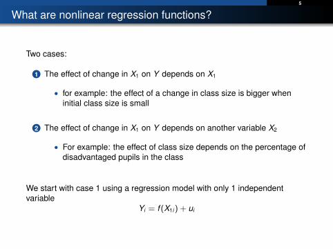
Two cases:
1 The effect of change in X1 on Y depends on X1
• for example: the effect of a change in class size is bigger wheninitial class size is small
2 The effect of change in X1 on Y depends on another variable X2
• For example: the effect of class size depends on the percentage ofdisadvantaged pupils in the class
We start with case 1 using a regression model with only 1 independentvariable
Yi = f (X1i) + ui
6
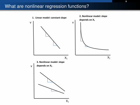
What are nonlinear regression functions?
2. Nonlinear model: slope
depends on X1
X1
X1
X1
Y
Y
Y
1. Linear model: constant slope
3. Nonlinear model: slope
depends on X2
7
Data
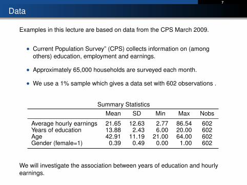
Examples in this lecture are based on data from the CPS March 2009.
• Current Population Survey” (CPS) collects information on (amongothers) education, employment and earnings.
• Approximately 65,000 households are surveyed each month.
• We use a 1% sample which gives a data set with 602 observations .
Summary StatisticsMean SD Min Max Nobs
Average hourly earnings 21.65 12.63 2.77 86.54 602Years of education 13.88 2.43 6.00 20.00 602Age 42.91 11.19 21.00 64.00 602Gender (female=1) 0.39 0.49 0.00 1.00 602
We will investigate the association between years of education and hourlyearnings.
8
0
20
40
60
80
Ave
rage
hou
rly e
arni
ngs
5 6 7 8 9 10 11 12 13 14 15 16 17 18 19 20
Years of education
Thursday February 6 13:36:41 2014 Page 1
___ ____ ____ ____ ____(R) /__ / ____/ / ____/ ___/ / /___/ / /___/ Statistics/Data Analysis
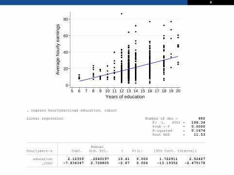
1 . regress hourlyearnings education, robust
Linear regression Number of obs = 602 F( 1, 600) = 108.34 Prob > F = 0.0000 R-squared = 0.1674 Root MSE = 11.53
Robusthourlyearn~s Coef. Std. Err. t P>|t| [95% Conf. Interval]
education 2.12359 .2040197 10.41 0.000 1.722911 2.52427 _cons -7.834347 2.728805 -2.87 0.004 -13.19352 -2.475178
9
Linear model: interpretation
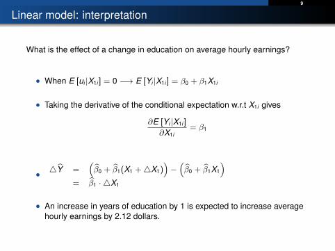
What is the effect of a change in education on average hourly earnings?
• When E [ui |X1i ] = 0 −→ E [Yi |X1i ] = β0 + β1X1i
• Taking the derivative of the conditional expectation w.r.t X1i gives
∂E [Yi |X1i ]
∂X1i= β1
• 4Y =(β0 + β1(X1 +4X1)
)−(β0 + β1X1
)= β1 · 4X1
• An increase in years of education by 1 is expected to increase averagehourly earnings by 2.12 dollars.
10
Polynomials
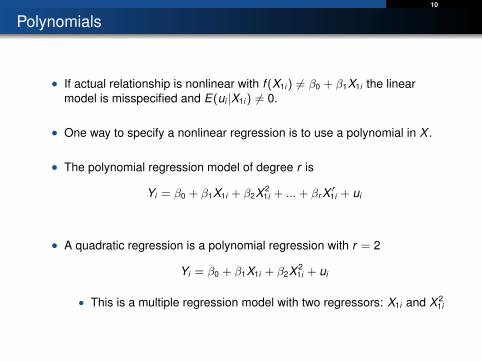
• If actual relationship is nonlinear with f (X1i) 6= β0 + β1X1i the linearmodel is misspecified and E(ui |X1i) 6= 0.
• One way to specify a nonlinear regression is to use a polynomial in X .
• The polynomial regression model of degree r is
Yi = β0 + β1X1i + β2X 21i + ...+ βr X r
1i + ui
• A quadratic regression is a polynomial regression with r = 2
Yi = β0 + β1X1i + β2X 21i + ui
• This is a multiple regression model with two regressors: X1i and X 21i
11
0
20
40
60
80
Ave
rage
hou
rly e
arni
ngs
5 6 7 8 9 10 11 12 13 14 15 16 17 18 19 20
Years of education
Thursday February 6 14:16:26 2014 Page 1
___ ____ ____ ____ ____(R) /__ / ____/ / ____/ ___/ / /___/ / /___/ Statistics/Data Analysis
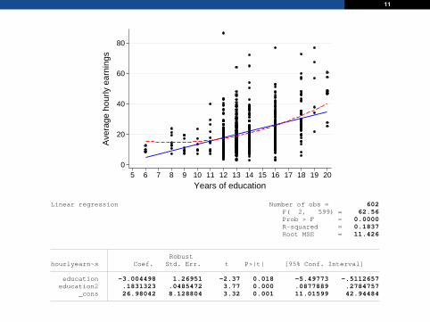
Linear regression Number of obs = 602 F( 2, 599) = 62.56 Prob > F = 0.0000 R-squared = 0.1837 Root MSE = 11.426
Robusthourlyearn~s Coef. Std. Err. t P>|t| [95% Conf. Interval]
education -3.004498 1.26951 -2.37 0.018 -5.49773 -.5112657 education2 .1831323 .0485472 3.77 0.000 .0877889 .2784757 _cons 26.98042 8.128804 3.32 0.001 11.01599 42.94484
12
Polynomials: interpretation
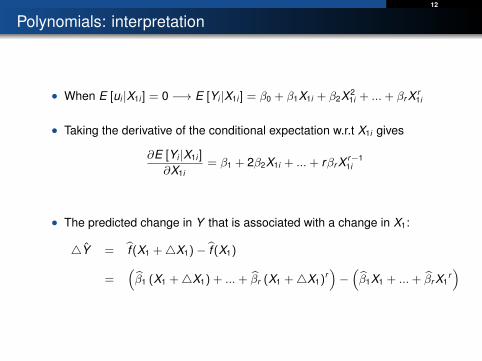
• When E [ui |X1i ] = 0 −→ E [Yi |X1i ] = β0 + β1X1i + β2X 21i + ...+ βr X r
1i
• Taking the derivative of the conditional expectation w.r.t X1i gives
∂E [Yi |X1i ]
∂X1i= β1 + 2β2X1i + ...+ rβr X r−1
1i
• The predicted change in Y that is associated with a change in X1:
4Y = f (X1 +4X1)− f (X1)
=(β1 (X1 +4X1) + ...+ βr (X1 +4X1)
r)−(β1X1 + ...+ βr X1
r)
13
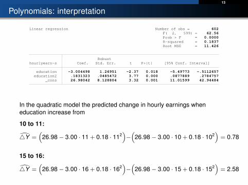
Polynomials: interpretation
Thursday February 6 14:16:26 2014 Page 1
___ ____ ____ ____ ____(R) /__ / ____/ / ____/ ___/ / /___/ / /___/ Statistics/Data Analysis
Linear regression Number of obs = 602 F( 2, 599) = 62.56 Prob > F = 0.0000 R-squared = 0.1837 Root MSE = 11.426
Robusthourlyearn~s Coef. Std. Err. t P>|t| [95% Conf. Interval]
education -3.004498 1.26951 -2.37 0.018 -5.49773 -.5112657 education2 .1831323 .0485472 3.77 0.000 .0877889 .2784757 _cons 26.98042 8.128804 3.32 0.001 11.01599 42.94484
In the quadratic model the predicted change in hourly earnings wheneducation increase from
10 to 11:
4Y =(
26.98− 3.00 · 11 + 0.18 · 112)−(
26.98− 3.00 · 10 + 0.18 · 102)= 0.78
15 to 16:
4Y =(
26.98− 3.00 · 16 + 0.18 · 162)−(
26.98− 3.00 · 15 + 0.18 · 152)= 2.58
14
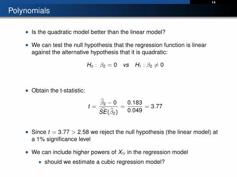
Polynomials
• Is the quadratic model better than the linear model?
• We can test the null hypothesis that the regression function is linearagainst the alternative hypothesis that it is quadratic:
Ho : β2 = 0 vs H1 : β2 6= 0
• Obtain the t-statistic:
t =β2 − 0
SE(β2)=
0.1830.049
= 3.77
• Since t = 3.77 > 2.58 we reject the null hypothesis (the linear model) ata 1% significance level
• We can include higher powers of X1i in the regression model
• should we estimate a cubic regression model?
15
Polynomials Tuesday February 11 09:49:17 2014 Page 1
___ ____ ____ ____ ____(R) /__ / ____/ / ____/ ___/ / /___/ / /___/ Statistics/Data Analysis
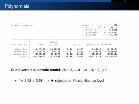
1 . regress hourlyearnings education education2 education3, robust
Linear regression Number of obs = 602 F( 3, 598) = 55.01 Prob > F = 0.0000 R-squared = 0.1933 Root MSE = 11.368
Robusthourlyearn~s Coef. Std. Err. t P>|t| [95% Conf. Interval]
education 14.20664 5.252381 2.70 0.007 3.89128 24.52199 education2 -1.165764 .437365 -2.67 0.008 -2.024722 -.3068056 education3 .0338681 .0115973 2.92 0.004 .0110918 .0566444 _cons -43.01427 19.90841 -2.16 0.031 -82.11317 -3.915365
Cubic versus quadratic model: Ho : β3 = 0 vs H1 : β3 6= 0
• t = 2.92 > 2.58 −→ H0 rejected at 1% significance level
16
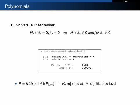
Polynomials
Cubic versus linear model:
Ho : β2 = 0, β3 = 0 vs H1 : β2 6= 0 and/or β2 6= 0 Tuesday February 11 09:50:02 2014 Page 1
___ ____ ____ ____ ____(R) /__ / ____/ / ____/ ___/ / /___/ / /___/ Statistics/Data Analysis
1 . test education2=education3=0
( 1) education2 - education3 = 0 ( 2) education2 = 0
F( 2, 598) = 8.39 Prob > F = 0.0003
• F = 8.39 > 4.61(F2,∞) −→ H0 rejected at 1% significance level
17
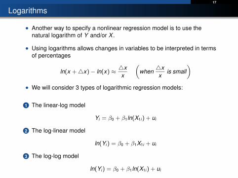
Logarithms
• Another way to specify a nonlinear regression model is to use thenatural logarithm of Y and/or X .
• Using logarithms allows changes in variables to be interpreted in termsof percentages
ln(x +4x)− ln(x) ≈ 4xx
(when
4xx
is small)
• We will consider 3 types of logarithmic regression models:
1 The linear-log model
Yi = β0 + β1ln(X1i) + ui
2 The log-linear model
ln(Yi) = β0 + β1X1i + ui
3 The log-log model
ln(Yi) = β0 + β1ln(X1i) + ui
18
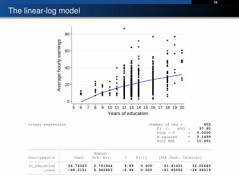
The linear-log model
0
20
40
60
80
Ave
rage
hou
rly e
arni
ngs
5 6 7 8 9 10 11 12 13 14 15 16 17 18 19 20
Years of education
Friday February 7 12:13:58 2014 Page 1
___ ____ ____ ____ ____(R) /__ / ____/ / ____/ ___/ / /___/ / /___/ Statistics/Data Analysis
Linear regression Number of obs = 602 F( 1, 600) = 97.80 Prob > F = 0.0000 R-squared = 0.1499 Root MSE = 11.651
Robusthourlyearn~s Coef. Std. Err. t P>|t| [95% Conf. Interval]
ln_education 26.72023 2.701844 9.89 0.000 21.41401 32.02645 _cons -48.2151 6.942683 -6.94 0.000 -61.85002 -34.58019
19
The linear-log model: interpretation
• When E [ui |X1i ] = 0 −→ E [Yi |X1i ] = β0 + β1ln(X1i)
• Taking the derivative of the conditional expectation w.r.t X1i gives
∂E [Yi |X1i ]
∂X1i= β1 ·
1X1i
• Using that ∂E [Yi |X1i ]∂X1i
≈ 4E [Yi |X1i ]4X1i
for small changes in X1 and rewritinggives
4E [Yi |X1i ] ≈ β1 ·4X1i
X1i
• Interpretation of β1: A 1% change in X1 (4X1iX1i
= 0.01) is associatedwith a change in Y of 0.01β1
• A 1 % increase in years of education is expected to increase averagehourly earnings by 0.27 dollars
20
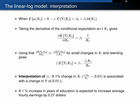
The log-linear model
0
1
2
3
4
5
Loga
ritm
of a
vera
ge h
ourly
ear
ning
s
5 6 7 8 9 10 11 12 13 14 15 16 17 18 19 20
Years of education
Friday February 7 12:17:11 2014 Page 1
___ ____ ____ ____ ____(R) /__ / ____/ / ____/ ___/ / /___/ / /___/ Statistics/Data Analysis
1 . regress ln_hourlyearnings education, robust
Linear regression Number of obs = 602 F( 1, 600) = 139.52 Prob > F = 0.0000 R-squared = 0.1571 Root MSE = .52602
Robustln_hourlye~s Coef. Std. Err. t P>|t| [95% Conf. Interval]
education .0932827 .0078974 11.81 0.000 .0777728 .1087927 _cons 1.622094 .1112224 14.58 0.000 1.403662 1.840527
21
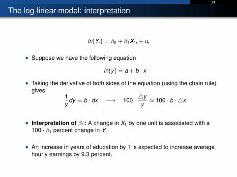
The log-linear model: interpretation
ln(Yi) = β0 + β1X1i + ui
• Suppose we have the following equation
ln(y) = a + b · x
• Taking the derivative of both sides of the equation (using the chain rule)gives
1y
dy = b · dx −→ 100 · 4yy≈ 100 · b · 4x
• Interpretation of β1: A change in X1 by one unit is associated with a100 · β1 percent change in Y
• An increase in years of education by 1 is expected to increase averagehourly earnings by 9.3 percent.
22
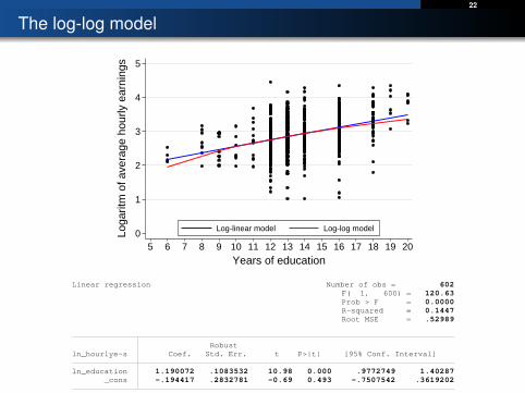
The log-log model
0
1
2
3
4
5
Loga
ritm
of a
vera
ge h
ourly
ear
ning
s
5 6 7 8 9 10 11 12 13 14 15 16 17 18 19 20
Years of education
Log-linear model Log-log model Friday February 7 12:48:45 2014 Page 1
___ ____ ____ ____ ____(R) /__ / ____/ / ____/ ___/ / /___/ / /___/ Statistics/Data Analysis
Linear regression Number of obs = 602 F( 1, 600) = 120.63 Prob > F = 0.0000 R-squared = 0.1447 Root MSE = .52989
Robustln_hourlye~s Coef. Std. Err. t P>|t| [95% Conf. Interval]
ln_education 1.190072 .1083532 10.98 0.000 .9772749 1.40287 _cons -.194417 .2832781 -0.69 0.493 -.7507542 .3619202
23
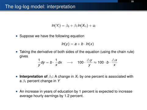
The log-log model: interpretation
ln(Yi) = β0 + β1ln(X1i) + ui
• Suppose we have the following equation
ln(y) = a + b · ln(x)
• Taking the derivative of both sides of the equation (using the chain rule)gives
1y
dy = b · 1x
dx −→ 100 · 4yy≈ 100 · b · 4x
x
• Interpretation of β1: A change in X1 by one percent is associated witha β1 percent change in Y
• An increase in years of education by 1 percent is expected to increaseaverage hourly earnings by 1.2 percent.
24
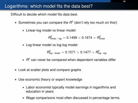
Logarithms: which model fits the data best?
Difficult to decide which model fits data best.
• Sometimes you can compare the R2 (don’t rely too much on this!)
• Linear-log model vs linear model:
R2linear−log = 0.1499 < 0.1674 = R2
linear
• Log-linear model vs log-log model:
R2log−linear = 0.1571 > 0.1477 = R2
log−log
• R2 can never be compared when dependent variables differ
• Look at scatter plots and compare graphs
• Use economic theory or expert knowledge
• Labor economist typically model earnings in logarithms andeducation in years
• Wage comparisons most often discussed in percentage terms.
25
Interactions
• So far we discussed nonlinear models with 1 independent variable X1i
• We now turn to models whereby the effect of X1i depends on anothervariable X2i
• We discuss 3 cases:
1 Interactions between two binary variables
2 Interactions between a binary and a continuous variable
3 Interactions between two continuous variables
26
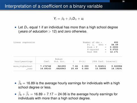
Interpretation of a coefficient on a binary variable
Yi = β0 + β1D1i + ui
• Let D1i equal 1 if an individual has more than a high school degree(years of education > 12) and zero otherwise.
Monday February 10 14:33:44 2014 Page 1
___ ____ ____ ____ ____(R) /__ / ____/ / ____/ ___/ / /___/ / /___/ Statistics/Data Analysis
1 . regress hourlyearnings more_highschool, robust
Linear regression Number of obs = 602 F( 1, 600) = 58.09 Prob > F = 0.0000 R-squared = 0.0723 Root MSE = 12.171
Robust hourlyearnings Coef. Std. Err. t P>|t| [95% Conf. Interval]
more_highschool 7.172748 .941093 7.62 0.000 5.324511 9.020984 _cons 16.89143 .6626943 25.49 0.000 15.58995 18.19291
• β0 = 16.89 is the average hourly earnings for individuals with a highschool degree or less.
• β0 + β1 = 16.89 + 7.17 = 24.06 is the average hourly earnings forindividuals with more than a high school degree.
27
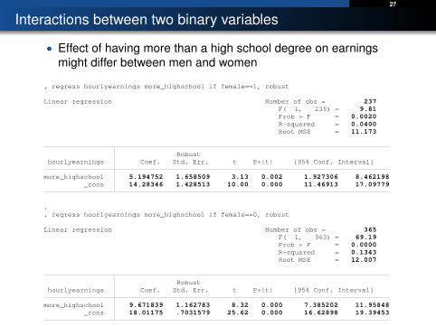
Interactions between two binary variables
• Effect of having more than a high school degree on earningsmight differ between men and women
Monday February 10 14:34:29 2014 Page 1
___ ____ ____ ____ ____(R) /__ / ____/ / ____/ ___/ / /___/ / /___/ Statistics/Data Analysis
1 . regress hourlyearnings more_highschool if female==1, robust
Linear regression Number of obs = 237 F( 1, 235) = 9.81 Prob > F = 0.0020 R-squared = 0.0400 Root MSE = 11.173
Robust hourlyearnings Coef. Std. Err. t P>|t| [95% Conf. Interval]
more_highschool 5.194752 1.658509 3.13 0.002 1.927306 8.462198 _cons 14.28346 1.428513 10.00 0.000 11.46913 17.09779
2 . 3 . regress hourlyearnings more_highschool if female==0, robust
Linear regression Number of obs = 365 F( 1, 363) = 69.19 Prob > F = 0.0000 R-squared = 0.1343 Root MSE = 12.007
Robust hourlyearnings Coef. Std. Err. t P>|t| [95% Conf. Interval]
more_highschool 9.671839 1.162783 8.32 0.000 7.385202 11.95848 _cons 18.01175 .7031579 25.62 0.000 16.62898 19.39453
28
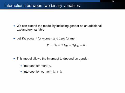
Interactions between two binary variables
• We can extend the model by including gender as an additionalexplanatory variable
• Let D2i equal 1 for women and zero for men
Yi = β0 + β1D1i + β2D2i + ui
• This model allows the intercept to depend on gender
• intercept for men: β0
• intercept for women: β0 + β2
29
Interactions between two binary variables Tuesday February 11 10:32:24 2014 Page 1
___ ____ ____ ____ ____(R) /__ / ____/ / ____/ ___/ / /___/ / /___/ Statistics/Data Analysis
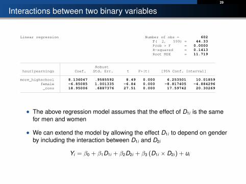
Linear regression Number of obs = 602 F( 2, 599) = 44.33 Prob > F = 0.0000 R-squared = 0.1413 Root MSE = 11.719
Robust hourlyearnings Coef. Std. Err. t P>|t| [95% Conf. Interval]
more_highschool 8.136047 .9585592 8.49 0.000 6.253501 10.01859 female -6.85085 1.001335 -6.84 0.000 -8.817405 -4.884296 _cons 18.95006 .6887376 27.51 0.000 17.59742 20.30269
• The above regression model assumes that the effect of D1i is the samefor men and women
• We can extend the model by allowing the effect D1i to depend on genderby including the interaction between D1i and D2i
Yi = β0 + β1D1i + β2D2i + β3 (D1i × D2i) + ui
30
Interactions between two binary variables
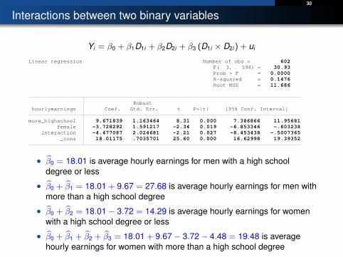
Yi = β0 + β1D1i + β2D2i + β3 (D1i × D2i) + ui
Monday February 10 14:56:49 2014 Page 1
___ ____ ____ ____ ____(R) /__ / ____/ / ____/ ___/ / /___/ / /___/ Statistics/Data Analysis
Linear regression Number of obs = 602 F( 3, 598) = 30.93 Prob > F = 0.0000 R-squared = 0.1476 Root MSE = 11.686
Robust hourlyearnings Coef. Std. Err. t P>|t| [95% Conf. Interval]
more_highschool 9.671839 1.163464 8.31 0.000 7.386866 11.95681 female -3.728292 1.591217 -2.34 0.019 -6.853346 -.603238 interaction -4.477087 2.024681 -2.21 0.027 -8.453438 -.5007365 _cons 18.01175 .7035701 25.60 0.000 16.62998 19.39352
• β0 = 18.01 is average hourly earnings for men with a high schooldegree or less
• β0 + β1 = 18.01 + 9.67 = 27.68 is average hourly earnings for men withmore than a high school degree
• β0 + β2 = 18.01− 3.72 = 14.29 is average hourly earnings for womenwith a high school degree or less
• β0 + β1 + β2 + β3 = 18.01 + 9.67− 3.72− 4.48 = 19.48 is averagehourly earnings for women with more than a high school degree
31
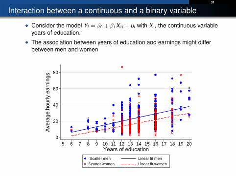
Interaction between a continuous and a binary variable
• Consider the model Yi = β0 + β1X1i + ui with X1i the continuous variableyears of education.
• The association between years of education and earnings might differbetween men and women
0
20
40
60
80
Ave
rage
hou
rly e
arni
ngs
5 6 7 8 9 10 11 12 13 14 15 16 17 18 19 20Years of education
Scatter men Linear fit menScatter women Linear fit women
32
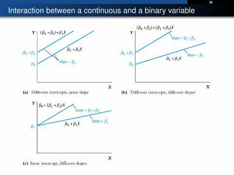
Interaction between a continuous and a binary variable
Copyright © 2011 Pearson Addison-Wesley. All rights reserved.
Binary-continuous interactions, ctd.
8-45
33
Interaction between a continuous and a binary variable
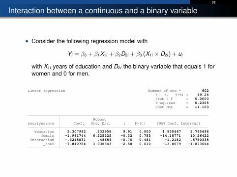
• Consider the following regression model with
Yi = β0 + β1X1i + β2D2i + β3 (X1i × D2i) + ui
with X1i years of education and D2i the binary variable that equals 1 forwomen and 0 for men.
Monday February 10 16:37:02 2014 Page 1
___ ____ ____ ____ ____(R) /__ / ____/ / ____/ ___/ / /___/ / /___/ Statistics/Data Analysis
Linear regression Number of obs = 602 F( 3, 598) = 49.24 Prob > F = 0.0000 R-squared = 0.2305 Root MSE = 11.103
Robusthourlyearn~s Coef. Std. Err. t P>|t| [95% Conf. Interval]
education 2.307982 .232958 9.91 0.000 1.850467 2.765498 female -1.961744 6.225225 -0.32 0.753 -14.18771 10.26422 interaction -.3215831 .45654 -0.70 0.481 -1.2182 .5750335 _cons -7.840784 3.038343 -2.58 0.010 -13.8079 -1.873664
1 . test female=interaction=0
( 1) female - interaction = 0 ( 2) female = 0
F( 2, 598) = 25.23 Prob > F = 0.0000
2 .
34
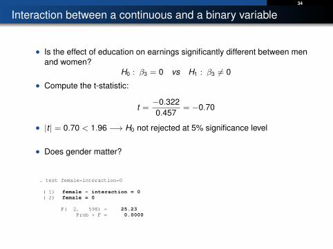
Interaction between a continuous and a binary variable
• Is the effect of education on earnings significantly different between menand women?
H0 : β3 = 0 vs H1 : β3 6= 0
• Compute the t-statistic:
t =−0.3220.457
= −0.70
• |t | = 0.70 < 1.96 −→ H0 not rejected at 5% significance level
• Does gender matter?
Monday February 10 16:37:02 2014 Page 1
___ ____ ____ ____ ____(R) /__ / ____/ / ____/ ___/ / /___/ / /___/ Statistics/Data Analysis
Linear regression Number of obs = 602 F( 3, 598) = 49.24 Prob > F = 0.0000 R-squared = 0.2305 Root MSE = 11.103
Robusthourlyearn~s Coef. Std. Err. t P>|t| [95% Conf. Interval]
education 2.307982 .232958 9.91 0.000 1.850467 2.765498 female -1.961744 6.225225 -0.32 0.753 -14.18771 10.26422 interaction -.3215831 .45654 -0.70 0.481 -1.2182 .5750335 _cons -7.840784 3.038343 -2.58 0.010 -13.8079 -1.873664
1 . test female=interaction=0
( 1) female - interaction = 0 ( 2) female = 0
F( 2, 598) = 25.23 Prob > F = 0.0000
2 .
35
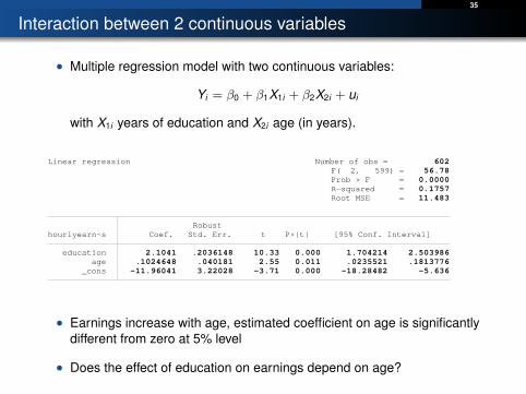
Interaction between 2 continuous variables
• Multiple regression model with two continuous variables:
Yi = β0 + β1X1i + β2X2i + ui
with X1i years of education and X2i age (in years).
Tuesday February 11 11:17:58 2014 Page 1
___ ____ ____ ____ ____(R) /__ / ____/ / ____/ ___/ / /___/ / /___/ Statistics/Data Analysis
Linear regression Number of obs = 602 F( 2, 599) = 56.78 Prob > F = 0.0000 R-squared = 0.1757 Root MSE = 11.483
Robusthourlyearn~s Coef. Std. Err. t P>|t| [95% Conf. Interval]
education 2.1041 .2036148 10.33 0.000 1.704214 2.503986 age .1024648 .040181 2.55 0.011 .0235521 .1813776 _cons -11.96041 3.22028 -3.71 0.000 -18.28482 -5.636
• Earnings increase with age, estimated coefficient on age is significantlydifferent from zero at 5% level
• Does the effect of education on earnings depend on age?
36
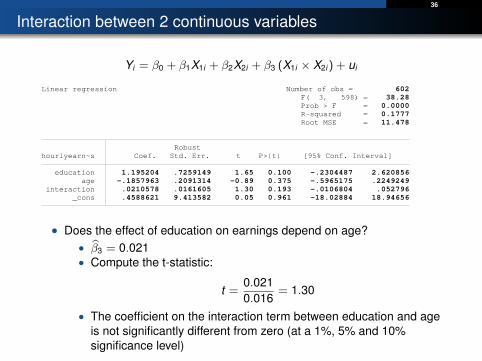
Interaction between 2 continuous variables
Yi = β0 + β1X1i + β2X2i + β3 (X1i × X2i) + ui
Tuesday February 11 11:23:25 2014 Page 1
___ ____ ____ ____ ____(R) /__ / ____/ / ____/ ___/ / /___/ / /___/ Statistics/Data Analysis
Linear regression Number of obs = 602 F( 3, 598) = 38.28 Prob > F = 0.0000 R-squared = 0.1777 Root MSE = 11.478
Robusthourlyearn~s Coef. Std. Err. t P>|t| [95% Conf. Interval]
education 1.195204 .7259149 1.65 0.100 -.2304487 2.620856 age -.1857963 .2091314 -0.89 0.375 -.5965175 .2249249 interaction .0210578 .0161605 1.30 0.193 -.0106804 .052796 _cons .4588621 9.413582 0.05 0.961 -18.02884 18.94656
• Does the effect of education on earnings depend on age?• β3 = 0.021• Compute the t-statistic:
t =0.0210.016
= 1.30
• The coefficient on the interaction term between education and ageis not significantly different from zero (at a 1%, 5% and 10%significance level)
37
Concluding remarks
• We discussed nonlinear regression models
Yi = f (X1i ,X2i , .....,Xki) + ui
• Models that are nonlinear in the independent variables are variants ofthe multiple regression model
• and can therefore be estimated by OLS,
• t- and F-tests can be used to test hypothesis about the values ofthe coefficients,
• provided that the OLS assumptions hold (topic of next week)
• Often difficult to decide which (non)linear model best fits the data
• Make a scatter plot
• Use t- and F-tests
• Use economic knowledge and intuition.