introductory map theory, by yanpei liu
DESCRIPTION
As an introductory work, this book contains the elementary materials in map theory, includingembeddings of a graph, abstract maps, duality, orientable and non-orientable maps, isomorphisms of maps and the enumeration of rooted or unrooted maps, particularly, thejoint tree representation of an embedding of a graph on two dimensional manifolds, whichenables one to make the complication much simpler on map enumeration. All of theseare valuable for researchers and students in combinatorics, graphs and low dimensionaltopology.A Smarandache system (Sigma;R) is such a mathematical system with at leastone Smarandachely denied rule r in R such that it behaves in at least two different wayswithin the same set Sigma, i.e., validated and invalided, or only invalided but in multiple distinctways. A map is a 2-cell decomposition of surface, which can be seen as a connectedgraphs in development from partition to permutation, also a basis for constructing Smarandachesystems, particularly, Smarandache 2-manifolds for Smarandache geometries.TRANSCRIPT

YANPEI LIU
INTRODUCTORY MAP THEORY
Kapa & Omega, Glendale, AZ
USA
2010

Yanpei LIU
Institute of Mathematics
Beijing Jiaotong University
Beijing 100044, P.R.China
Email: [email protected]
Introductory Map Theory
Kapa & Omega, Glendale, AZ
USA
2010
This book can be ordered in a paper bound reprint from:
Books on Demand
ProQuest Information & Learning
(University of Microfilm International)
300 N.Zeeb Road
P.O.Box 1346, Ann Arbor
MI 48106-1346, USA
Tel:1-800-521-0600(Customer Service)
http://wwwlib.umi.com/bod
Peer Reviewers:
L.F.Mao, Chinese Academy of Mathematics and System Science, P.R.China.
J.L.Cai, Beijing Normal University, P.R.China.
H.Ren, East China Normal University, P.R.China.
R.X.Hao, Beijing Jiaotong University, P.R.China.
Copyright 2010 by Kapa & Omega, Glendale, AZ and Yanpei Liu
Many books can be downloaded from the following Digital Library of Science:
http://www.gallup.unm.edu/∼smarandache/eBooks-otherformats.htm
ISBN: 978-1-59973-134-6
Printed in America

Preface
Maps as a mathematical topic arose probably from the four color
problem[Bir1, Ore1] and the more general map coloring problem[HiC1,
Rin1, Liu11] in the mid of nineteenth century although maps as poly-
hedra which go back to the Platonic age. I could not list references
in detail on them because it is well known for a large range of readers
and beyond the scope of this book. Here, I only intend to present
a comprehensive theory of maps as a rigorous mathematical concept
which has been developed mostly in the last half a century.
However, as described in the book[Liu15] maps can be seen as
graphs in development from partition to permutation and as a basis
extended to Smarandache geometry shown in [Mao3–4]. This is why
maps are much concerned with abstraction in the present stage.
In the beginning, maps as polyhedra were as a topological, or ge-
ometric object even with geographical consideration[Kem1]. The first
formal definition of a map was done by Heffter from [Hef1] in the 19th
century. However, it was not paid an attention by mathematicians
until 1960 when Edmonds published a note in the AMS Notices with
the dual form of Heffter’s in [Edm1,Liu3].
Although this concept was widely used in literature as [Liu1–2,
Liu4–6, Rin1–3, Sta1–2, et al], its disadvantage for the nonorientable
case involved does not bring with some convenience for clarifying some
related mathematical thinking.
Since Tutte described the nonorientability in a new way [Tut1–
3], a number of authors begin to develop it in combinatorization of
continuous objects as in [Lit1, Liu7–10, Vin1–2, et al].
The above representations are all with complication in construct-
ing an embedding, or all distinct embeddings of a graph on a surface.

iv Preface
However, the joint tree model of an embedding completed in recent
years and initiated from the early articles at the end of seventies in
the last century by the present author as shown in [Liu1–2] enables us
to make the complication much simpler.
Because of the generality that an asymmetric object can always
be seen with some local symmetry in certain extent, the concepts of
graphs and maps are just put in such a rule. In fact, the former is
corresponding to that a group of two elements sticks on an edge and
the later is that a group of four elements sticks on an edge such that
a graph without symmetry at all is in company with local symmetry.
This treatment will bring more advantages for observing the structure
of a graph. Of course, the later is with restriction of the former because
of the later as a permutation and the former as a partition.
The joint tree representation of an embedding of a graph on
two dimensional manifolds, particularly surfaces(compact 2-manifolds
without boundary in our case), is described in Chapter I for simplifying
a number of results old and new.
This book contains the following chapters in company with re-
lated subjects.
In Chapter I, the embedding of a graph on surfaces are much
concerned because they are motivated to building up the theory of
abstract maps related with Smarandache geometry.
The second chapter is for the formal definition of abstract maps.
One can see that this matter is a natural generalization of graph em-
bedding on surfaces.
The third chapter is on the duality not only for maps themselves
but also for operations on maps from one surface to another. One
can see how the duality is naturally deduced from the abstract maps
described in the second chapter.
The fourth chapter is on the orientability. One can see how the
orientability is formally designed as a combinatorial invariant. The
fifth chapter concentrates on the classification of orientable maps. The
sixth chapter is for the classification of nonorientable maps.
From the two chapters: Chapter V and Chapter VI, one can see

Preface v
how the procedure is simplified for these classifications.
The seventh chapter is on the isomorphisms of maps and pro-
vides an efficient algorithm for the justification and recognition of the
isomorphism of two maps, which has been shown to be useful for de-
termining the automorphism group of a map in the eighth chapter.
Moreover, it enables us to access an automorphism of a graph.
The ninth and the tenth chapters observe the number of distinct
asymmetric maps with the size as a parameter. In the former, only
one vertex maps are counted by favorite formulas and in the latter,
general maps are counted from differential equations. More progresses
about this kind of counting are referred to read the recent book[Liu7]
and many further articles[Bax1, BeG1, CaL1–2, ReL1–3, etc].
The next chapter, Chapter XI, only presents some ideas for ac-
cessing the symmetric census of maps and further, of graphs. This
topic is being developed in some other directions[KwL1–2] and left as
a subject written in the near future.
From Chapter XII through Chapter XV, extensions from basic
theory are much concerned with further applications.
Chapter XII discusses in brief on genus polynomial of a graph
and all its super maps rooted and unrooted on the basis of the joint
tree model. Recent progresses on this aspect are referred to read the
articles [Liu13–15, LiP1, WaL1–2, ZhL1–2, ZuL1, etc].
Chapter XIII is on the census of maps with vertex or face par-
titions. Although such census involves with much complication and
difficulty, because of the recent progress on a basic topic about trees
via an elementary method firstly used by the author himself we are
able to do a number of types of such census in very simple way. This
chapter reflects on such aspects around.
Chapter XIV is on graphs that their super maps are particularly
considered for asymmetrical and symmetrical census via their semi-
automorphism and automorphism groups or via embeddings of graphs
given [Liu19, MaL1, MaT1, MaW1, etc].
Chapter XV, is on functional equations discovered in the census
of a variety of maps on sphere and general surfaces. Although their

vi Preface
well definedness has been done, almost all of them have not yet been
solved up to now.
Three appendices are compliment to the context. One provides
the clarification of the concepts of polyhedra, surfaces, embeddings,
and maps and their relationship. The other two are for exhaustively
calculating numerical results and listing all rooted and unrooted maps
for small graphs with more calculating results compared with those
appearing in [Liu14], [Liu17] and [Liu19].
From a large amount of materials, more than hundred observa-
tions for beginners probably senior undergraduates, more than hun-
dred exercises for mainly graduates of master degree and more than
hundred research problems for mainly graduates of doctoral degree are
carefully designed at the end of each chapter in adapting the needs of
such a wide range of readers for mastering, extending and investigat-
ing a number of ways to get further development on the basic theory
of abstract maps.
Although I have been trying to design this book self contained as
much as possible, some books such as [DiM1], [Mss1] and [GaJ1] might
be helpful to those not familiar with basic knowledge of permutation
groups, topology and computing complexity as background.
Since early nineties of the last century, a number of my former
and present graduates were or are engaged with topics related to this
book. Among them, I have to mention Dr. Ying Liu[LpL1], Dr. Yuan-
qiu Huang[HuL1], Dr. Junliang Cai[CaL1–2], Dr. Deming Li[LiL1],
Dr. Han Ren[ReL1–3], Dr. Rongxia Hao[HaC1, HaL1], Dr. Zhaox-
iang Li[LiQ1–2], Dr. Linfan Mao[MaL1, MaT1, MaW1], Dr. Er-
ling Wei[WiL1–2], Dr. Weili He[HeL1], Dr. Liangxia Wan[WaL1–2],
Dr. Yichao Chen[CnL1, CnR1], Dr. Yan Xu[XuL1–2], Dr. Wen-
zhong Liu[LwL1–2], Dr. Zeling Shao[ShL1], Dr. Yan Yang[YaL1–2],
Dr. Guanghua Dong[DoL1], Ms. Ximei Zhao[ZhL1–2], Mr. Lifeng
Li[LiP1], Ms. Huiyan Wang[WgL1], Ms. Zhao Chai[CiL1], Mr. Zi-
long Zhu[ZuL1], et al for their successful work related to this book.
On this occasion, I should express my heartiest appreciation of
the financial support by KOSEF of Korea from the Com2MaC (Com-

Preface vii
binatorial and Computational Mathematics Research Center) of the
Pohang University of Science and Technology in the summer of 2001.
In that period, the intention of this book was established. Moreover,
I should be also appreciated to the Natural Science Foundation of
China for the research development reflected in this book under its
Grants(60373030, 10571013, 10871021).
Y.P. Liu
Beijing, China
Jan., 2010

Contents
Preface . . . . . . . . . . . . . . . . . . . . . . . . . . . . . . . . . . . . . . . . . . . . . . . . . . . . . . . . . iii
Chapter I Abstract Embeddings . . . . . . . . . . . . . . . . . . . . . . . . . . . .1
I.1 Graphs and networks . . . . . . . . . . . . . . . . . . . . . . . . . . . . . . . . . . . 1
I.2 Surfaces . . . . . . . . . . . . . . . . . . . . . . . . . . . . . . . . . . . . . . . . . . . . . . . . 9
I.3 Embeddings . . . . . . . . . . . . . . . . . . . . . . . . . . . . . . . . . . . . . . . . . . . 16
I.4 Abstract representation . . . . . . . . . . . . . . . . . . . . . . . . . . . . . . . . 22
I.5 Smarandache 2-manifolds with map geometry . . . . . . . . . 27
Activities on Chapter I . . . . . . . . . . . . . . . . . . . . . . . . . . . . . . . . . 32
I.6 Observations . . . . . . . . . . . . . . . . . . . . . . . . . . . . . . . . . . . . . . . . . . 32
I.7 Exercises . . . . . . . . . . . . . . . . . . . . . . . . . . . . . . . . . . . . . . . . . . . . . . 34
I.8 Researches. . . . . . . . . . . . . . . . . . . . . . . . . . . . . . . . . . . . . . . . . . . . .37
Chapter II Abstract Maps . . . . . . . . . . . . . . . . . . . . . . . . . . . . . . . . 41
II.1 Ground sets . . . . . . . . . . . . . . . . . . . . . . . . . . . . . . . . . . . . . . . . . . 41
II.2 Basic permutations . . . . . . . . . . . . . . . . . . . . . . . . . . . . . . . . . . . 43
II.3 Conjugate axiom . . . . . . . . . . . . . . . . . . . . . . . . . . . . . . . . . . . . . 46
II.4 Transitive axiom. . . . . . . . . . . . . . . . . . . . . . . . . . . . . . . . . . . . . . 49
II.5 Included angles . . . . . . . . . . . . . . . . . . . . . . . . . . . . . . . . . . . . . . . 55
Activities on Chapter II . . . . . . . . . . . . . . . . . . . . . . . . . . . . . . . . 57
II.6 Observations. . . . . . . . . . . . . . . . . . . . . . . . . . . . . . . . . . . . . . . . . .57
II.7 Exercises . . . . . . . . . . . . . . . . . . . . . . . . . . . . . . . . . . . . . . . . . . . . . 58
II.8 Researches . . . . . . . . . . . . . . . . . . . . . . . . . . . . . . . . . . . . . . . . . . . . 59
Chapter III Duality . . . . . . . . . . . . . . . . . . . . . . . . . . . . . . . . . . . . . . . . .65
III.1 Dual maps . . . . . . . . . . . . . . . . . . . . . . . . . . . . . . . . . . . . . . . . . . 65

x Contents
III.2 Deletion of an edge . . . . . . . . . . . . . . . . . . . . . . . . . . . . . . . . . . 72
III.3 Addition of an edge . . . . . . . . . . . . . . . . . . . . . . . . . . . . . . . . . . 85
III.4 Basic transformation . . . . . . . . . . . . . . . . . . . . . . . . . . . . . . . . . 96
Activities on Chapter III . . . . . . . . . . . . . . . . . . . . . . . . . . . . . . . 98
III.5 Observations . . . . . . . . . . . . . . . . . . . . . . . . . . . . . . . . . . . . . . . . . 98
III.6 Exercises . . . . . . . . . . . . . . . . . . . . . . . . . . . . . . . . . . . . . . . . . . . . 99
III.7 Researches . . . . . . . . . . . . . . . . . . . . . . . . . . . . . . . . . . . . . . . . . . 101
Chapter IV Orientability . . . . . . . . . . . . . . . . . . . . . . . . . . . . . . . . 103
IV.1 Orientation . . . . . . . . . . . . . . . . . . . . . . . . . . . . . . . . . . . . . . . . 103
IV.2 Basic equivalence . . . . . . . . . . . . . . . . . . . . . . . . . . . . . . . . . . . 107
IV.3 Euler characteristic . . . . . . . . . . . . . . . . . . . . . . . . . . . . . . . . . 113
IV.4 Pattern examples . . . . . . . . . . . . . . . . . . . . . . . . . . . . . . . . . . . 116
Activities on Chapter IV . . . . . . . . . . . . . . . . . . . . . . . . . . . . . . 119
IV.5 Observations. . . . . . . . . . . . . . . . . . . . . . . . . . . . . . . . . . . . . . . .119
IV.6 Exercises . . . . . . . . . . . . . . . . . . . . . . . . . . . . . . . . . . . . . . . . . . . 120
IV.7 Researches . . . . . . . . . . . . . . . . . . . . . . . . . . . . . . . . . . . . . . . . . . 122
Chapter V Orientable Maps . . . . . . . . . . . . . . . . . . . . . . . . . . . . . .124
V.1 Butterflies . . . . . . . . . . . . . . . . . . . . . . . . . . . . . . . . . . . . . . . . . . 124
V.2 Simplified butterflies . . . . . . . . . . . . . . . . . . . . . . . . . . . . . . . . . 126
V.3 Reduced rules . . . . . . . . . . . . . . . . . . . . . . . . . . . . . . . . . . . . . . . 130
V.4 Orientable principles. . . . . . . . . . . . . . . . . . . . . . . . . . . . . . . . .134
V.5 Orientable genus. . . . . . . . . . . . . . . . . . . . . . . . . . . . . . . . . . . . .137
Activities on Chapter V . . . . . . . . . . . . . . . . . . . . . . . . . . . . . . . 139
V.6 Observations . . . . . . . . . . . . . . . . . . . . . . . . . . . . . . . . . . . . . . . . 139
V.7 Exercises . . . . . . . . . . . . . . . . . . . . . . . . . . . . . . . . . . . . . . . . . . . . 140
V.8 Researches. . . . . . . . . . . . . . . . . . . . . . . . . . . . . . . . . . . . . . . . . . .142
Chapter VI Nonorientable Maps . . . . . . . . . . . . . . . . . . . . . . . .145
VI.1 Barflies . . . . . . . . . . . . . . . . . . . . . . . . . . . . . . . . . . . . . . . . . . . . 145

Contents xi
VI.2 Simplified barflies . . . . . . . . . . . . . . . . . . . . . . . . . . . . . . . . . . . 149
VI.3 Nonorientable rules . . . . . . . . . . . . . . . . . . . . . . . . . . . . . . . . . 151
VI.4 Nonorientable principles . . . . . . . . . . . . . . . . . . . . . . . . . . . . 156
VI.5 Nonorientable genus . . . . . . . . . . . . . . . . . . . . . . . . . . . . . . . . 157
Activities on Chapter VI . . . . . . . . . . . . . . . . . . . . . . . . . . . . . . 159
VI.5 Observations. . . . . . . . . . . . . . . . . . . . . . . . . . . . . . . . . . . . . . . .159
VI.6 Exercises . . . . . . . . . . . . . . . . . . . . . . . . . . . . . . . . . . . . . . . . . . . 160
VI.7 Researches . . . . . . . . . . . . . . . . . . . . . . . . . . . . . . . . . . . . . . . . . . 162
Chapter VII Isomorphisms of Maps . . . . . . . . . . . . . . . . . . . . 164
VII.1 Commutativity . . . . . . . . . . . . . . . . . . . . . . . . . . . . . . . . . . . . 164
VII.2 Isomorphism theorem . . . . . . . . . . . . . . . . . . . . . . . . . . . . . . 168
VII.3 Recognition . . . . . . . . . . . . . . . . . . . . . . . . . . . . . . . . . . . . . . . . 172
VII.4 Justification . . . . . . . . . . . . . . . . . . . . . . . . . . . . . . . . . . . . . . . 177
VII.5 Pattern examples . . . . . . . . . . . . . . . . . . . . . . . . . . . . . . . . . . 180
Activities on Chapter VII . . . . . . . . . . . . . . . . . . . . . . . . . . . . .185
VII.6 Observations . . . . . . . . . . . . . . . . . . . . . . . . . . . . . . . . . . . . . . . 185
VII.7 Exercises . . . . . . . . . . . . . . . . . . . . . . . . . . . . . . . . . . . . . . . . . . 186
VII.8 Researches . . . . . . . . . . . . . . . . . . . . . . . . . . . . . . . . . . . . . . . . . 188
Chapter VIII Asymmetrization . . . . . . . . . . . . . . . . . . . . . . . . . 190
VIII.1 Automorphisms . . . . . . . . . . . . . . . . . . . . . . . . . . . . . . . . . . . 190
VIII.2 Upper bound of group order. . . . . . . . . . . . . . . . . . . . . . .193
VIII.3 Determination of the group . . . . . . . . . . . . . . . . . . . . . . . 196
VIII.4 Rootings . . . . . . . . . . . . . . . . . . . . . . . . . . . . . . . . . . . . . . . . . . 201
Activities on Chapter VIII . . . . . . . . . . . . . . . . . . . . . . . . . . . .206
VIII.5 Observations . . . . . . . . . . . . . . . . . . . . . . . . . . . . . . . . . . . . . . 206
VIII.6 Exercises. . . . . . . . . . . . . . . . . . . . . . . . . . . . . . . . . . . . . . . . . .207
VIII.7 Researches . . . . . . . . . . . . . . . . . . . . . . . . . . . . . . . . . . . . . . . . 209

xii Contents
Chapter IX Rooted Petal Bundles . . . . . . . . . . . . . . . . . . . . . . .212
IX.1 Orientable petal bundles . . . . . . . . . . . . . . . . . . . . . . . . . . . . 212
IX.2 Planar pedal bundles . . . . . . . . . . . . . . . . . . . . . . . . . . . . . . . 217
IX.3 Nonorientable pedal bundles . . . . . . . . . . . . . . . . . . . . . . . . 220
IX.4 The number of pedal bundles . . . . . . . . . . . . . . . . . . . . . . . 226
Activities on Chapter IX . . . . . . . . . . . . . . . . . . . . . . . . . . . . . . 230
IX.5 Observations. . . . . . . . . . . . . . . . . . . . . . . . . . . . . . . . . . . . . . . .230
IX.6 Exercises . . . . . . . . . . . . . . . . . . . . . . . . . . . . . . . . . . . . . . . . . . . 231
IX.7 Researches . . . . . . . . . . . . . . . . . . . . . . . . . . . . . . . . . . . . . . . . . . 232
Chapter X Asymmetrized Maps . . . . . . . . . . . . . . . . . . . . . . . . . 235
X.1 Orientable equation. . . . . . . . . . . . . . . . . . . . . . . . . . . . . . . . . .235
X.2 Planar rooted maps. . . . . . . . . . . . . . . . . . . . . . . . . . . . . . . . . .243
X.3 Nonorientable equation . . . . . . . . . . . . . . . . . . . . . . . . . . . . . . 250
X.4 Gross equation . . . . . . . . . . . . . . . . . . . . . . . . . . . . . . . . . . . . . . 255
X.5 The number of rooted maps . . . . . . . . . . . . . . . . . . . . . . . . . 258
Activities on Chapter X . . . . . . . . . . . . . . . . . . . . . . . . . . . . . . . 261
X.6 Observations . . . . . . . . . . . . . . . . . . . . . . . . . . . . . . . . . . . . . . . . 261
X.7 Exercises . . . . . . . . . . . . . . . . . . . . . . . . . . . . . . . . . . . . . . . . . . . . 262
X.8 Researches. . . . . . . . . . . . . . . . . . . . . . . . . . . . . . . . . . . . . . . . . . .265
Chapter XI Maps with Symmetry . . . . . . . . . . . . . . . . . . . . . . . 268
XI.1 Symmetric relation . . . . . . . . . . . . . . . . . . . . . . . . . . . . . . . . . 268
XI.2 An application . . . . . . . . . . . . . . . . . . . . . . . . . . . . . . . . . . . . . . 270
XI.3 Symmetric principle . . . . . . . . . . . . . . . . . . . . . . . . . . . . . . . . 272
XI.4 General examples . . . . . . . . . . . . . . . . . . . . . . . . . . . . . . . . . . . 274
Activities on Chapter XI . . . . . . . . . . . . . . . . . . . . . . . . . . . . . . 278
XI.5 Observations. . . . . . . . . . . . . . . . . . . . . . . . . . . . . . . . . . . . . . . .278
XI.6 Exercises . . . . . . . . . . . . . . . . . . . . . . . . . . . . . . . . . . . . . . . . . . . 279
XI.7 Researches . . . . . . . . . . . . . . . . . . . . . . . . . . . . . . . . . . . . . . . . . . 280

Contents xiii
Chapter XII Genus Polynomials . . . . . . . . . . . . . . . . . . . . . . . . . 282
XII.1 Associate surfaces . . . . . . . . . . . . . . . . . . . . . . . . . . . . . . . . . 282
XII.2 Layer division of a surface . . . . . . . . . . . . . . . . . . . . . . . . . 285
XII.3 Handle polymomials . . . . . . . . . . . . . . . . . . . . . . . . . . . . . . . 289
XII.4 Crosscap polynomials . . . . . . . . . . . . . . . . . . . . . . . . . . . . . . 290
Activities on Chapter XII . . . . . . . . . . . . . . . . . . . . . . . . . . . . .292
XII.5 Observations . . . . . . . . . . . . . . . . . . . . . . . . . . . . . . . . . . . . . . . 292
XII.6 Exercises . . . . . . . . . . . . . . . . . . . . . . . . . . . . . . . . . . . . . . . . . . 293
XII.7 Researches . . . . . . . . . . . . . . . . . . . . . . . . . . . . . . . . . . . . . . . . . 294
Chapter XIII Census with Partitions . . . . . . . . . . . . . . . . . . . .297
XIII.1 Planted trees . . . . . . . . . . . . . . . . . . . . . . . . . . . . . . . . . . . . . 297
XIII.2 Hamiltonian cubic maps . . . . . . . . . . . . . . . . . . . . . . . . . . 305
XIII.3 Halin maps . . . . . . . . . . . . . . . . . . . . . . . . . . . . . . . . . . . . . . . 307
XIII.4 Biboundary inner rooted maps . . . . . . . . . . . . . . . . . . . . 310
XIII.5 General maps . . . . . . . . . . . . . . . . . . . . . . . . . . . . . . . . . . . . . 315
XIII.6 Pan-flowers . . . . . . . . . . . . . . . . . . . . . . . . . . . . . . . . . . . . . . . 317
Activities on Chapter XIII . . . . . . . . . . . . . . . . . . . . . . . . . . . .323
XIII.7 Observations . . . . . . . . . . . . . . . . . . . . . . . . . . . . . . . . . . . . . . 323
XIII.8 Exercises. . . . . . . . . . . . . . . . . . . . . . . . . . . . . . . . . . . . . . . . . .324
XIII.9 Researches . . . . . . . . . . . . . . . . . . . . . . . . . . . . . . . . . . . . . . . . 325
Chapter XIV Super Maps of a Graph . . . . . . . . . . . . . . . . . . .326
XIV.1 Semi-automorphisms on a graph . . . . . . . . . . . . . . . . . . 326
XIV.2 Automorphisms on a graph . . . . . . . . . . . . . . . . . . . . . . . 329
XIV.3 Relationships . . . . . . . . . . . . . . . . . . . . . . . . . . . . . . . . . . . . . 332
XIV.4 Nonisomorphic super maps . . . . . . . . . . . . . . . . . . . . . . . . 334
XIV.5 Via rooted super maps . . . . . . . . . . . . . . . . . . . . . . . . . . . . 336
Activities on Chapter XIV . . . . . . . . . . . . . . . . . . . . . . . . . . . . 341
XIV.6 Observations . . . . . . . . . . . . . . . . . . . . . . . . . . . . . . . . . . . . . . 341

xiv Contents
XIV.7 Exercises . . . . . . . . . . . . . . . . . . . . . . . . . . . . . . . . . . . . . . . . . . 342
XIV.8 Researches . . . . . . . . . . . . . . . . . . . . . . . . . . . . . . . . . . . . . . . . 334
Chapter XV Equations with Partitions . . . . . . . . . . . . . . . . . 345
XV.1 The meson functional . . . . . . . . . . . . . . . . . . . . . . . . . . . . . 345
XV.2 General maps on the sphere . . . . . . . . . . . . . . . . . . . . . . . . 350
XV.3 Nonseparable maps on the sphere . . . . . . . . . . . . . . . . . . 353
XV.4 Maps without cut-edge on furfaces . . . . . . . . . . . . . . . . . 357
XV.5 Eulerian maps on the sphere . . . . . . . . . . . . . . . . . . . . . . . 361
XV.6 Eulerian maps on surfaces. . . . . . . . . . . . . . . . . . . . . . . . . .365
Activities on Chapter XV . . . . . . . . . . . . . . . . . . . . . . . . . . . . . 370
XV.7 Observations . . . . . . . . . . . . . . . . . . . . . . . . . . . . . . . . . . . . . . . 370
XV.8 Exercises . . . . . . . . . . . . . . . . . . . . . . . . . . . . . . . . . . . . . . . . . . 371
XV.9 Researches . . . . . . . . . . . . . . . . . . . . . . . . . . . . . . . . . . . . . . . . . 372
Appendix I Concepts of Polyhedra, Surfaces,
Embeddings and Maps . . . . . . . . . . . . . . . . . . . . . . . . . 374
Ax.I.1 Polyhedra. . . . . . . . . . . . . . . . . . . . . . . . . . . . . . . . . . . . . . . . .374
Ax.I.2 Surfaces . . . . . . . . . . . . . . . . . . . . . . . . . . . . . . . . . . . . . . . . . . 377
Ax.I.3 Embeddings . . . . . . . . . . . . . . . . . . . . . . . . . . . . . . . . . . . . . . 381
Ax.I.4 Maps . . . . . . . . . . . . . . . . . . . . . . . . . . . . . . . . . . . . . . . . . . . . . 384
Appendix II Table of Genus Polynomials for
Embeddings and Maps of Small Size . . . . . . . . . . . . 389
Ax.II.1 Triconnected cubic graphs. . . . . . . . . . . . . . . . . . . . . . . .389
Ax.II.2 Bouquets . . . . . . . . . . . . . . . . . . . . . . . . . . . . . . . . . . . . . . . . 398
Ax.II.3 Wheels. . . . . . . . . . . . . . . . . . . . . . . . . . . . . . . . . . . . . . . . . . .401
Ax.II.4 Link bundles . . . . . . . . . . . . . . . . . . . . . . . . . . . . . . . . . . . . . 403
Ax.II.5 Complete bipartite graphs. . . . . . . . . . . . . . . . . . . . . . . .405
Ax.II.6 Complete graphs . . . . . . . . . . . . . . . . . . . . . . . . . . . . . . . . . 407
Contents xv
Appendix III Atlas of Rooted and Unrooted Maps
for Small Graphs . . . . . . . . . . . . . . . . . . . . . . . . . . . . . . . 409
Ax.III.1 Bouquets Bm of size 4 ≥ m ≥ 1 . . . . . . . . . . . . . . . . . 409
Ax.III.2 Link bundles Lm of size 7 ≥ m ≥ 3 . . . . . . . . . . . . . . 415
Ax.III.3 Complete bipartite graphs Km,n, 4 ≥ m,n ≥ 3 . . . 432
Ax.III.4 Wheels Wn of order 6 ≥ n ≥ 4. . . . . . . . . . . . . . . . . . .437
Ax.III.5 Complete graphs Kn, 5 ≥ n ≥ 4 . . . . . . . . . . . . . . . . . 447
Ax.III.6 Triconnected cubic graphs of size in [6, 15] . . . . . . . 452
Bibliography . . . . . . . . . . . . . . . . . . . . . . . . . . . . . . . . . . . . . . . . . . . . . . . . . 472
Terminology . . . . . . . . . . . . . . . . . . . . . . . . . . . . . . . . . . . . . . . . . . . . . . . . . 480

Chapter I
Abstract Embeddings
• A graph is considered as a partition on the union of sets obtained
from each element of a given set the binary group B = 0, 1 sticks
on.
• A surface, i.e., a compact 2-manifold without boundary in topol-
ogy, is seen as a polygon of even edges pairwise identified.
• An embedding of a graph on a surface is represented by a joint
tree of the graph. A joint of a graph consists of a plane extended
tree with labelled cotree semi-edges. Two semi-edges of a cotree
edge has the same label as the cotree edge with a binary index.
An extended tree is compounded of a spanning tree with cotree
semi-edges.
• Combinatorial properties of an embedding in abstraction are par-
ticularly discussed for the formal definition of a map.
I.1 Graphs and networks
LetX be a finite set. For any x ∈ X, the binary group B = 0, 1sticks on x to obtain Bx = x(0), x(1). x(0) and x(1) are called the
ends of x, or Bx. If Bx is seen as an ordered set 〈x(0), x(1)〉, then

2 Chapter I Abstract Embeddings
x(0) and x(1) are, respectively,initial and terminal ends of x. Let
X =∑
x∈XBx, (1.1)
i.e., the disjoint union of all Bx, x ∈ X. X is called the ground set.
A (directed) pregraph is a partition Par= P1, P2, · · · of the
ground set X ,i.e.,
X =∑
i≥1
Pi. (1.2)
Bx (or 〈x(0), x(1)〉), or simply denoted by x itself, x ∈ X, is called an
(arc) edge and Pi, i ≥ 1, a node or vertex.
A (directed) pregraph is written as G = (V,E) where V =Par
and
E = B(X) = Bx|x ∈ X
(= 〈x(0), x(1)〉|x ∈ X).
If X is a finite set, the (directed) pregraph is called finite; otherwise,
infinite. In this book, (directed) pregraphs are all finite.
If X = ∅, then the (directed) pregraph is said to be empty as
well.
An edge (arc) is considered to have two semiedges each of them
is incident with only one end (semiarcs with directions of one from
the end and the other to the end). An edge (arc) is with two ends
identified is called a selfloop (di-selfloop); otherwise, a link (di-link). If
t edges (arcs) have same ends (same direction) are called a multiedge
(multiarc), or t-edge (t-arc).
Example 1.1 There are two directed pregraphs on X = x,i.e.,
Par1 = x(0), x(1);
Par2 = x(0), x(1).
They are all distinct pregraphs as well as shown in Fig.1.1.

I.1 Graphs and networks 3>x +x
Par1 Par2
Fig.1.1 Directed pregraphs of 1 edge
Further, pregraphs of size 2 are observed.
Example 1.2 On X = x1, x2, the 15 directed pregraphs are
as follows:
Par1 = x1(0), x1(1), x2(0), x2(1);Par2 = x1(0), x1(1), x2(0), x2(1);Par3 = x1(0), x2(0), x1(1), x2(1);Par4 = x1(0), x2(1), x1(1), x2(0);Par5 = x1(0), x1(1), x2(0), x2(1);Par6 = x1(0), x1(1), x2(1), x2(0);Par7 = x1(0), x1(1), x2(1), x2(0);Par8 = x1(0), x1(1), x2(0), x2(1);Par9 = x1(0), x1(1), x2(1), x2(0);Par10 = x1(0), x2(0), x2(1), x1(1);Par11 = x1(0), x1(1), x2(0), x2(1);Par12 = x1(0), x1(1), x2(0), x2(1);Par13 = x1(0), x1(1), x2(0), x2(1);Par14 = x1(0), x2(0), x1(1), x2(1);Par15 = x1(0), x2(1), x1(1), x2(0).
Among the 15 directed pregraphs, Par3, Par4, Par5 and Par6
are 1 pregraph; Par8 and Par9 are 1 pregraph; Par10 and Par11 are 1
pregraph; Par14 and Par15 are 1 pregraph; and others are 1 pregraph
each. Thus, there are 9 pregraphs in all(as shown in Fig.1.2).

4 Chapter I Abstract Embeddings x1 x2 x1 x2
M x1 x2
Par1 Par2 Par3
/M x1 x2 N x1 x2 /Nx1 x2
Par4 Par5 Par6
x1 x2 N x1 x2 ?x1 x2
Par7 Par8 Par9
Mx1 x2 Nx1 x2 ? x1
x2
Par10 Par11 Par12? x1x2 -6x1
x2
-x1
x2
Par13 Par14 Par15
Fig.1.2 Directed pregraphs of 2 edges
Now, Par= P1, P2, · · · and B are, respectively, seen as a map-
ping z 7→ Pi, z ∈ Pi, i ≥ 1 and a mapping z 7→ z, z 6= z, z, z ∈B(X). The composition of two mappings α and β on a set Z is defined
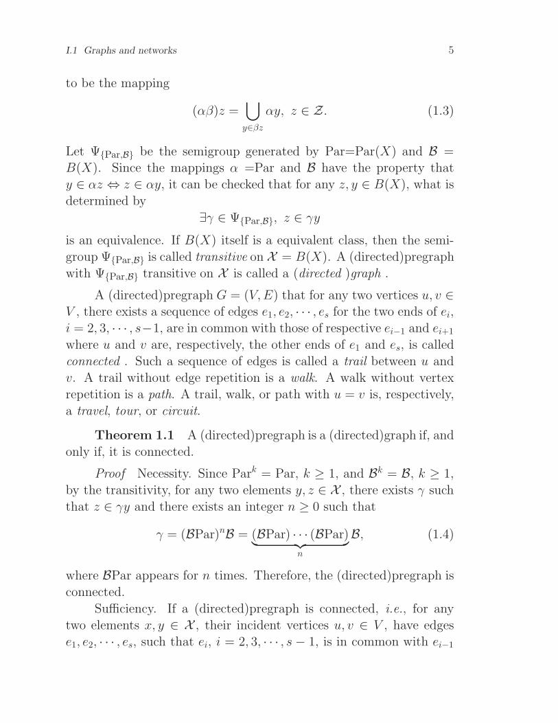
I.1 Graphs and networks 5
to be the mapping
(αβ)z =⋃
y∈βz
αy, z ∈ Z. (1.3)
Let ΨPar,B be the semigroup generated by Par=Par(X) and B =
B(X). Since the mappings α =Par and B have the property that
y ∈ αz ⇔ z ∈ αy, it can be checked that for any z, y ∈ B(X), what is
determined by
∃γ ∈ ΨPar,B, z ∈ γyis an equivalence. If B(X) itself is a equivalent class, then the semi-
group ΨPar,B is called transitive on X = B(X). A (directed)pregraph
with ΨPar,B transitive on X is called a (directed )graph .
A (directed)pregraph G = (V,E) that for any two vertices u, v ∈V , there exists a sequence of edges e1, e2, · · · , es for the two ends of ei,
i = 2, 3, · · · , s−1, are in common with those of respective ei−1 and ei+1
where u and v are, respectively, the other ends of e1 and es, is called
connected . Such a sequence of edges is called a trail between u and
v. A trail without edge repetition is a walk. A walk without vertex
repetition is a path. A trail, walk, or path with u = v is, respectively,
a travel, tour, or circuit.
Theorem 1.1 A (directed)pregraph is a (directed)graph if, and
only if, it is connected.
Proof Necessity. Since Park = Par, k ≥ 1, and Bk = B, k ≥ 1,
by the transitivity, for any two elements y, z ∈ X , there exists γ such
that z ∈ γy and there exists an integer n ≥ 0 such that
γ = (BPar)nB = (BPar) · · · (BPar)︸ ︷︷ ︸n
B, (1.4)
where BPar appears for n times. Therefore, the (directed)pregraph is
connected.
Sufficiency. If a (directed)pregraph is connected, i.e., for any
two elements x, y ∈ X , their incident vertices u, v ∈ V , have edges
e1, e2, · · · , es, such that ei, i = 2, 3, · · · , s− 1, is in common with ei−1

6 Chapter I Abstract Embeddings
and ei+1. Of course, u and v are, respectively, the ends of e1 and es.
Thus, y ∈ γz whereγ = (ParB)sB. This implies that the semigroup
ΨPar,B is transitive on X . Therefore, the (directed)pregraph is a
(directed)graph.
It is seen from the theorem that (directed) graphs here are, in
fact, connected (directed) graphs in most textbooks. Because discon-
nectedness is rarely necessary to consider, for convenience all graphs,
embeddings and then maps in what follows are defined within con-
nectedness in this book.
A network N is such a graph G = (V,E) with a real function
w(e) ∈ R, e ∈ E on E, and hence write N = (G;w). Usually, a
network N is denoted by the graph G itself if no confusion occurs.
Finite recursion principle On a finite set A, choose a0 ∈ Aas the initial element at the 0th step. Assume ai is chosen at the ith,
i ≥ 0, step with a given rule. If not all elements available from ai are
not yet chosen, choose one of them as ai+1 at the i + 1st step by the
rule, then a chosen element will be encountered in finite steps unless
all elements of A are chosen.
Finite restrict recursion principle On a finite set A, choose
a0 ∈ A as the initial element at the 0th step. Assume ai is chosen at
the ith, i ≥ 0, step with a given rule. If a0 is not available from ai,
choose one of elements available from ai as ai+1 at the i+ 1st step by
the rule, then a0 will be encountered in finite steps unless all elements
of A are chosen.
The two principles above are very useful in finite sets, graphs and
networks, even in a wide range of combinatorial optimizations.
A G = (V,E) with V = V1 + V2 of both V1 and V2 independent,
i.e., its vertex set is partitioned into two parts with each part having
no pair of vertices adjacent, is called bipartite.
Theorem 1.2 A graph G = (V,E) is bipartite if, and only if,
G has no circuit with odd number of edges.
Proof Necessity. Since G is bipartite, start from v0 ∈ V ini-

I.1 Graphs and networks 7
tially chosen and then by the rule from the vertex just chosen to one
of its adjacent vertices via an edge unused and then marked by used,
according to the finite recursion principle, an even circuit (from bipar-
tite), or no circuit at all, can be found. From the arbitrariness of v0
and the way going on, no circuit of G is with odd number of edges.
Sufficiency. Since all circuits are even, start from marking an
arbitrary vertex by 0 and then by the rule from a vertex marked
by b ∈ B = 0, 1 to mark all its adjacent vertices by b = 1 − b,
according to the finite recursion principle the vertex set is partitioned
into V0 = v ∈ V | marked by 0 and V1 = v ∈ V | marked by 1. By
the rule, V0 and V1 are both independent and hence G is bipartite.
From this theorem, a graph without circuit is bipartite. In fact,
from the transitivity, any graph without circuit is a tree.
On a pregraph, the number of elements incident to a vertex is
called the degree of the vertex. A pregraph of all vertices with even
degree is said to be even . If an even pregraph is a graph, then it is
called a Euler graph.
Theorem 1.3 A pregraph G = (V,E) is even if, and only if,
there exist circuits C1, C2, · · · , Cn, on G such that
E = C1 + C2 + · · ·+ Cn, (1.5)
where n is a nonnegative integer.
Proof Necessity. Since all the degrees of vertices on G are even,
any pregraph obtained by deleting the edges of a circuit from G is still
even. From the finite recursion principle, there exist a nonnegative
integer n and circuits C1, C2, · · · , Cn, on G such that (1.5) is satisfied.
Sufficiency. Because a circuit contributes 2 to the degree of each
of its incident vertices, (1.5) guarantees each of vertices on G has even
degree. Hence, G is even.
The set of circuits Ci|1 ≤ i ≤ n of G in (1.5) is called a
circuit partition, or written as Cir=Cir(G). Two direct conclusions of
Theorem 1.3 are very useful . One is the case that G is a graph. The

8 Chapter I Abstract Embeddings
other is for G is a directed pregraph. Their forms and proofs are left
for the reader.
Let N = (G;w) be a network where G = (V,E) and w(e) =
−w(e) ∈ Zn = 0, 1, · · · , n − 1, i.e., mod n, n ≥ 1, integer group.
For examples, Z1 = 0, Z2 = B = 0, 1 etc. Suppose xv = −xv ∈Zn, v ∈ V , are variables. Let us discuss the system of equations
xu + xv = w(e) (mod n), e = (u, v) ∈ E (1.6)
on Zn.
Theorem 1.4 System of equations(1.6) has a solution on Zn
if, and only if, there is no circuit C such that
∑
e∈Cw(e) 6= 0 (mod n) (1.7)
on N .
Proof Necessity. Assume C is a circuit satisfying (1.7) on N .
Because the restricted part of (1.6) on C has no solution, the whole
system of equations (1.6) has to be no solution either. Therefore, N
has no such circuit. This is a contradiction to the assumption
Sufficiency. Let x0 = a ∈ Zn, start from v0 ∈ V reached. Assume
vi ∈ V reached and xi = ai at step i. Choose one of ei = (vi, vi+1) ∈ Ewithout used(otherwise, backward 1 step as the step i). Choose vi+1
reached and ei used with ai+1 = ai + w(ei) at step i + 1. If a circuit
as e0, e1, · · · , el, ej = (vj, vj+1), 0 ≤ j ≤ l, vl+1 = v0, occurs within a
permutation of indices, then from (1.7)
al+1 = al + w(el)
= al−1 + w(el−1) + w(el)
· · · · · ·
= a0 +
l∑
j=0
w(ej)
= a0.

I.2 Surfaces 9
Because the system of equations obtained by deleting all the equations
for all the edges on the circuit from (1.6) is equivalent to the original
system of equations (1.6), in virtue of the finite recursion principle a
solution of (1.6) can always be extracted .
When n = 2, this theorem has a variety of applications. In [Liu5],
some applications can be seen. Further, its extension on a nonAbelian
group can also be done while the system of equations are not yet linear
but quadratic.
I.2 Surfaces
In topology, a surface is a compact 2-dimensional manifold with-
out boundary. In fact, it can be seen as what is obtained by identifying
each pair of edges on a polygon of even edges pairwise.
For example, in Fig.1.3, two ends of each dot line are the same
point. The left is a sphere, or the plane when the infinity is seen as
a point. The right is the projective plane. From the symmetry of the
sphere, a surface can also seen as a sphere cutting off a polygon with
pairwise edges identified.
The two surfaces in Fig.1.3 are formed by a polygon of two edges
pairwise as a.
Ra
a
I Ra
a
Sphere(Plane) Projective plane
Fig.1.3 Sphere and projective plane

10 Chapter I Abstract Embeddings
Surface closed curve axiom A closed curve on a surface has
one of the two possibilities: one side and two sides.
A curve with two sides is called a double side curve ; otherwise, a
single side curve . As shown in Fig.1.3, any closed curve on a sphere is
a double side curve(In fact, this is the Jordan curve axiom). However,
it is different from the sphere for the projective plane. there are both
a single(shown by a dot line) and a double side curve.
How do we justify whether a closed curve on a surface is of single
side, or not?
In order to answer this question, the concept of contractibility
of a curve has to be clarified. If a closed curve on a surface can be
continuously contracted along one side into a point, then it is said to
be contractible, or homotopic to 0.6 6----
a
a
b b
6 -?
a
a
b
b
Torus Klein bottle
Fig.1.4 Torus and Klein bottle
It is seen that a single side curve is never homotopic to 0 and
a double side curve is not always homotopic to 0. For example, in
Fig.1.4, the left, i.e., the torus, each of the dot lines is of double side
but not contractible. The right, i.e., the Klein bottle, all the dot lines
are of single side , and hence, none of them is contractible.
A surface with all closed curves of double side is called orientable;
otherwise, nonorientable .
For example, in Fig.1.3, the sphere is orientable and the projec-

I.2 Surfaces 11
tive plane is nonorientable. In Fig.1.4, the torus is orientable and the
Klein bottle is nonorientable.
The maximum number of closed curves cutting along without
destroying the continuity on a surface is called the pregenus of the
surface.
In view of Jordan curve axiom, there is no such closed curve on
the sphere. Thus, the pregenus of sphere is 0. On the projective plane,
only one such curve is available (each of dot lines is such a closed curve
in Fig.1.3) and hence the pregenus of projective plane is 1.
Similarly, the pregenera of torus and Klein bottle are both 2 as
shown in Fig.1.4.
Theorem 1.5 The pregenus of an orientable surface is a non-
negative even number.
A formal proof can not be done until Chapter 5. Based on this
theorem, the genus of an orientable surface can be defined to be half
its pregenus, called the orientable genus. The genus of a nonorientable
surface, called nonorientable genus, is its pregenus itself.
The sphere is written as aa−1 where a−1 is with the opposite
direction of a on the boundary of the polygon. Thus, the projective
plane, torus and Klein bottle are, respectively, aa, aba−1b−1 and aabb.
In general,
Op =
p∏
i=1
aibia−1i b−1
i
= a1b1a−11 b−1
1 a2b2a−12 b−1
2 · · · apbpa−1p b−1
p
(1.8)
and
Qq =
q∏
i=1
aiai = a1a1a2a2 · · · aqaq (1.9)
denote, respectively, a surface of orientable genus p and a surface of
nonorientable genus q. Of course, O0, Q1, O1 and Q2 are, respectively,
the sphere, projective plane, torus and Klein bottle.
It is easily checked that whenever an even polygon is with a pair
of its edges in the same direction, the polygon represents a nonori-
12 Chapter I Abstract Embeddings
entable surface. Thus, all Op, p ≥ 0, orientable and all Qq, q ≥ 1, are
nonorientable.
Forms (1.8) and (1.9) are said to be standard.
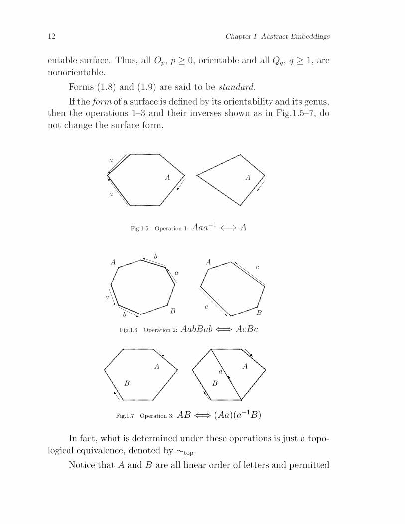
If the form of a surface is defined by its orientability and its genus,
then the operations 1–3 and their inverses shown as in Fig.1.5–7, do
not change the surface form.
.............................................................................................................................................................................................
..............
..............
......o A
a
a .............................................................................................................
...............................................................................
A /Fig.1.5 Operation 1: Aaa−1 ⇐⇒ A
...................................................................................................................................
..........................................................
................ iN ja
a
b
bA
B
...............................................
................................
........................
R
c
c
A
B
Fig.1.6 Operation 2: AabBab⇐⇒ AcBc
................................
....................................................................................................................................................
.......................................
B
A
R
................................
....................................................................................................................................................
.......................................
B
AK R a
Fig.1.7 Operation 3: AB ⇐⇒ (Aa)(a−1B)
In fact, what is determined under these operations is just a topo-
logical equivalence, denoted by ∼top.
Notice that A and B are all linear order of letters and permitted

I.2 Surfaces 13
to be empty as degenerate case in these operations.
The parentheses stand for cyclic order when more than one cyclic
orders occur for distinguishing from one to another.
Relation 0 On a surface (A,B), if A is a surface itself then
(A,B) = ((A)x(B)x−1) = ((A)(B)).
Relation 1 (AxByCx−1Dy−1) ∼top ((ADCB)(xyx−1y−1)).
Relation 2 (AxBx) ∼top ((AB−1)(xx)).
Relation 3 (Axxyzy−1z−1) ∼top ((A)(xx)(yy)(zz)).
In the four relations, A, B, C, and D are permitted to be empty.
B−1 = b−1s · · · b−1
3 b−12 b−1
1 is also called the inverse of B = b1b2b3 · · · bs,s ≥ 1. Parentheses are always omitted when unnecessary to distin-
guish cyclic or linear order.
On a surface S, the operation of cutting off a quadrangle aba−1b−1
and then identifying each pair of edges with the same letter is called
a handle as shown in the left of Fig.1.8.
If the quadrangle aba−1b−1 is replaced by aa, then such an oper-
ation is called a crosscap as shown in the right of Fig.1.8.-?? -a
a
b b
S RY a
a
S
Handle Crosscap
Fig.1.8 Handle and crosscap
The following theorem shows the result of doing a handle on an
orientable surface.
Theorem 1.6 What is obtained by doing a handle on an ori-
entable surface is still orientable with its genus 1 added.

14 Chapter I Abstract Embeddings
Proof Suppose S is the surface obtained, then
S ∼top
p∏
i=1
aibia−1i b−1
i xap+1bp+1a−1p+1b
−1p+1x
−1 ( Relation 0)
∼top
p∏
i=1
aibia−1i b−1
i xx−1ap+1bp+1a−1p+1b
−1p+1 (Relation 1)
∼top
p∏
i=1
aibia−1i b−1
i ap+1bp+1a−1p+1b
−1p+1 (Operation 1)
=
p+1∏
i=1
aibia−1i b−1
i .
This is the theorem.
In the above proof, x and x−1 are a line connecting the two
boundaries to represent the surface as a polygon shown in Fig.1.8.
This procedure can be seen as the degenerate case of operation 3.
In what follows, observe the result by doing a crosscap on an
orientable surface.
Theorem 1.7 On an orientable surface of genus p, p ≥ 0, what
is obtained by doing a crosscap is nonorientable with its genus 2p+ 1.
Proof Suppose N is the surface obtained, then
N ∼top
p∏
i=1
aibia−1i b−1
i xaax−1 (Relation 0)
∼top
p∏
i=1
aibia−1i b−1
i xx−1c1c1 (Relation 2)
∼top
p∏
i=2
aibia−1i b−1
i xx−1c1c1c2c2c3c3 (Relation 3)
∼top
2p+1∏
i=1
cici. (Relation 3 by p− 1 times).

I.2 Surfaces 15
This is the theorem.
By doing a handle on a nonorientable surface, 2 more genus
should be added with the same nonorientability.
Theorem 1.8 On a nonorientable surface, what is obtained by
doing a handle is nonorientable with its genus 2 added.
Proof Suppose N is the obtained surface, then
N ∼top
q∏
i=1
aiaixaba−1b−1x−1 (Relation 0)
∼top
q∏
i=1
aiaixx−1aba−1b−1 (Relation 1)
∼top
q∏
i=1
aiaiaba−1b−1 (Operation 1)
∼top
q+2∏
i=1
cici. (Relation 3).
This is the theorem.
By doing a crosscap on a nonorientable surface, 1 more genus
produced with the same nonorientability
Theorem 1.9 On a nonorientable surface, what is obtained by
doing a crosscap is nonorientable with its genus 1 added.

16 Chapter I Abstract Embeddings
Proof Suppose N is the obtained surface, then
N ∼top
q∏
i=1
aiaixaax−1 (Relation 0)
∼top
q∏
i=1
aiaixx−1aa (Relation 2)
∼top
q∏
i=1
aiaiaa (Operation 1)
∼top
q+1∏
i=1
aiai. (Relation 3).
This is the theorem.
I.3 Embedding
Let G = (V,E), V = v1, v2, · · · , vn, be a graph. A point in the
3-dimensional space is represented by a real number t as the parame-
ter, e.g., (x, y, z) = (t, t2, t3). Write the vertices as
vi = (xi, yi, zi) = (ti, t2i , t
3i )
such that ti 6= tj , i 6= j, 1 ≤ i, j ≤ n, and an edge as
(u, v) = u+ λv, 1 ≤ λ ≤ 1,
i.e., the straight line segment between u and v. Because for any four
vertices vi, vj, vl and vk,
det
(xi − xj xi − xl xi − xk
yi − yj yi − yl yi − yk
zi − zj zi − zl zi − zk
)
= det
ti − tj ti − tl ti − tkt2i − t2j t2i − t2l t2i − t2kt3i − t3j t3i − t3l t3i − t3k

I.3 Embedding 17
= (ti − tj)(ti − tl)(ti − tk)(tk − tl)(tk − tj)(tj − tl) 6= 0, i.e., the four
points are not coplanar, any two edges in G has no intersection inner
point.
A representation of a graph on a space with vertices as points
and edges as curves pairwise no intersection inner point is called an
embedding of the graph in the space. If all edges are straight line
segments in an embedding, then it is called a straight line embedding.
Thus, any graph has a straight line embedding in the 3-dimensional
space. Similarly, A surface embedding of graph G is a continuous
injection µG of an embedding of G on the 3-dimensional space to a
surface S such that each connected component of S−µG is homotopic
to 0. The connected component is called a face of the embedding. In
early books, a surface embedding is also called a cellular embedding.
Because only a surface embedding is concerned with in what follows,
an embedding is always meant a surface embedding if not necessary
to specify.
A graph without circuit is called a tree. A spanning tree of a
graph is such a subgraph that is a tree with the same order as the
graph. Usually, a spanning tree of a graph is in short called a tree on
the graph. For a tree on a graph, the numbers of edges on the tree
and not on the tree are only dependent on the order of the graph.
They are, respectively, called the rank and the corank of the graph.
The corank is also called the Betti number, or cyclic number by some
authors.
The following procedure can be used for finding an embedding
on a surface.
First, given a cyclic order of all semiedges at each vertex of G,
called a rotation. Find a tree(spanning, of course) T on G and distin-
guish all the edges not on T by letters. Then, replace each edge not
of T by two articulate edges with the same letter.
From this procedure, G is transformed into G without changing
the rotation at each vertex except for new vertices that are all ar-
ticulate. Because G is a tree, according to the rotation, all lettered
articulate edges of G form a polygon with β pairs of edges, and hence

18 Chapter I Abstract Embeddings
a surface in correspondence with a choice of indices on each pair of
the same letter. For convenience, G with a choice of indices of pair in
the same letter is called a joint tree of G.
Theorem 1.10 A graph G = (V,E) can always embedded into
a surface of orientable genus at most ⌊β/2⌋, or of nonorientable genus
at most β, where β is the Betti number of G.
Proof It is seen that any joint tree of G is an embedding of G
on the surface determined by its associate polygon. From (1.8) for
the orientable case, the surface has its genus at most ⌊2β/4⌋ = ⌊β/2⌋.From (1.9) for the nonorientable case, the surface has its genus at most
2β/2 = β.
In Fig.1.9, graph G and one of its joint tree are shown. Here, the
spanning tree T is represented by edges without letter. a, b and c are
edges not on T . Because the polygon is
abcacb ∼top c−1b−1cbaa (Relation 2)
∼top aabbcc (Theorem 1.7),
the joint tree is, in fact, an embedding of G on a nonorientable surface
of genus 3.
a
b c
a a
b
b
c
c
G G
Fig.1.9 Graph and its joint tree
Because any graph with given rotation can always immersed in
the plane in agreement with the rotation, each edge has two sides. As
known, embeddings of a graph on surfaces are distinguished by the
rotation of semiedges at each vertex and the choice of indices of the
two semiedges on each edge of the graph whenever edges are labelled

I.3 Embedding 19
by letters. Different indices of the two semiedges of an edge stand
for from one side of the edge to the other on a face boundary in an
embedding.
Theorem 1.11 A tree can only be embedded on the sphere.
Any graph G except tree can be embedded on a nonorientable surface.
Any graph G can always be embedded on an orientable surface. Let
nO(G) be the number of distinct embeddings on orientable surfaces,
then the number of embeddings on all surfaces is
2β(G)nO(G), nO(G) =∏
i≥2
((i− 1)!)ni, (1.10)
where β(G) is the Betti number and ni is the number of vertices of
degree i in G.
Proof On a surface of genus not 0, only a graph with at least
a circuit is possible to have an embedding. Because a tree has no
circuit, it can only embedded on the sphere. Because a graph not
a tree has at least one circuit, from Theorem 1.10 the second and
the third statements are true. Since distinct planar embeddings of a
joint tree of G with the indices of each letter different correspond to
distinct embeddings of G on orientable surfaces and the number of
distinct planar embeddings of joint trees is
nO(G) =∏
i≥2
((i− 1)!)ni.
Further, since the indices of letters on the β(G) edges has 2β(G) of
choices for a given orientable embedding and among them only one
choice corresponds to an orientable embedding, the fourth statement
is true.
For an embedding µ(G) of G on a surface, let ν(µG), ǫ(µG) and
φ(µG) are, respectively, its vertex number, or order, edge number, or
size and face number, or coorder.
Theorem 1.12 For a surface S, all embeddings µ(G) of a graph
G have Eul(µG) = ν(µG)− ǫ(µG) + φ(µG) the same, only dependent

20 Chapter I Abstract Embeddings
on S and independent of G. Further,
Eul(µG) =
2− 2p, p ≥ 0,
when S has orientable genus p;
2− q, q ≥ 1,
when S has nonorientable genus q.
(1.11)
Proof For an embedding µ(G) on S, if it has at least 2 faces,
then by connectedness it has 2 faces with a common edge. From the
finite recursion principle, by the inverse of Operation 3 an embedding
µ(G1) of G1 on S with only 1 face on S is found. It is easy to check
that Eul(µG) =Eul(µG1). Similarly, by the inverse of Operation 2 an
embedding µ(G0) of G0 on S with only 1 vertex is found. It is also
easy to check that Eul(µG) =Eul(µG′). Further, by Operation 1 and
Relations 1–3, it is seen that Eul(µG0) =Eul(Op), p ≥ 0; or Eul(Qq),
q ≥ 1 according as S is an orientable surface in (1.8); or not in (1.9).
From the arbitrariness of G, the first statement is proved.
By calculating the order, size and coorder of Op, p ≥ 0; or Qq,
q ≥ 1, (1.11) is soon obtained. So, the second statement is proved.
According to this theorem, for an embedding µ(G) of graph G,
Eul(µG) is called its Euler characteristic, or of the surface it is on.
Further, g(µG) is the genus of the surface µ(G) is on.
If a graph G is with the minimum length of circuits σ, then
from Theorem 1.12 the genus γ(G) of an orientable surface G can be
embedded on satisfies the inequality
1− ν(G)− ǫ(1− 2σ)
2≤ γ(G) ≤ ⌊β
2⌋ (1.12)
and the genus γ(G) of a nonorientable surface G can be embedded on
satisfies the inequality
2− (ν(G)− ǫ(1− 2
σ)) ≤ γ(G) ≤ β. (1.13)
If a graph has an embedding with its genus attaining the lower(upper)
bound in (1.12) and (1.13), then it is called down(up)-embeddable. In
I.3 Embedding 21
fact, a graph is up-embeddable on nonorientable, or orientable sur-
faces according as it has an embedding with only 1 face, or at most 2
faces.
Theorem 1.13 All graphs but trees are up-embeddable on
nonorientable surfaces.
Further, if a graph has an embedding of nonorientable genus l
and an embedding of nonorientable genus k, l < k, then for any i,
l < i < k, it has an embedding of nonorientable genus i.
Proof For an arbitrary embedding of a graph G on a nonori-
entable surface, let T be its corresponding joint tree. From the nonori-
entability, the associate 2β(G)-gon P has at least 1 letter with different
indices(or same power of its two occurrences!). If P = Qq, q = β(G),
then the embedding is an up-embedding in its own right. Otherwise,
by Relation 2, or Relation 3 if necessary, whenever s−1s or stst oc-
curs, it is, respectively, replaced by ss or sts−1t. In virtue of no letter
missed in the procedure, from the finite recursion principle, P ′ = Qq,
q = β(G), is obtained. This is the first statement.
From the arbitrariness of starting embedding in the procedure
of proving the first statement by only using Relation 2 instead of
Relation 3 (AststB ∼top Ass−1Btt by Relation 2), because the genus
of the surface is increased 1 by 1, the the second statement is true.
The second statement of this theorem is also called the inter-
polation theorem. The orientable form of interpolation theorem is
firstly given by Duke[Duk1]. The maximum(minimum) of the genus
of surfaces (orientable or nonorientable) a graph can be embedded
on is call the maximum genus(minimum genus) of the graph. The-
orem 1.13 shows that graphs but trees are all have their maximum
genus on nonorientable surfaces the Betti number with the interpola-
tion theorem. The proof would be the simplest one. However, for the
orientable case, it is far from simple. many results have been obtained
since 1978(see [Liu1–2], [LiuL1], [HuanL1] and [LidL1]) in this aspect.
On the determination of minimum genus of a graph, only a few of
graphs with certain symmetry are done(see Chapter 12 in [Liu5–6]).

22 Chapter I Abstract Embeddings
I.4 Abstract representation
Let G = (V,X), V = v1, v2, · · · , vn,
X = x1, x2, · · · , xm ⊆ V ×V = u, v|∀u, v ∈ V ,
be a graph. For an embedding µ(G) of G on a surface, each edge has
not only two ends as in G but also two sides. Let α be the operation
from one side to the other and β be the operation from one end to
the other. From the symmetry between the two ends and between the
two sides,
α2 = β2 = 1 (1.14)
where 1 is the identity. By considering that the result from one side
to the other and then to the other end and the result from one end to
the other and then to the other side are the same, i.e.,
βα = αβ. (1.15)
Further, it can be seen that K = 1, α, β, γ, γ = αβ, is a group,
called the Klein group where
(αβ)2 = (αβ)(αβ) = (αβα)β
= (ααβ)β = (αα)(ββ) = 1.(1.16)
Thus, an edge x ∈ X of G in an embedding µ(G) of G becomes
Kx = x, αx, βx, γx, as shown in Fig.1.10.-- x βx
αx αβx
Fig.1.10 An edge sticking on K
In fact, let
X =
m∑
i=1
Kxi (1.17)

I.4 Abstract representation 23
where summation stands for the disjoint union, then α and β can both
be seen as a permutation on X , i.e.,
α =m∏
i=1
(xi, αxi)(βxi, γxi), β =m∏
i=1
(xi, βxi)(αxi, γxi).
The vertex x is on deals with the rotation as
(x,Px,P2x, · · ·), (αx, αP−1x, αP−2x, · · ·), (1.18)
as shown in Fig.1.11(when its degree is 4).
--x
αx
βx
αβx -- P2x
αP2x
βP2x
αβP2x
66??Px αPx
βPx αβP2x
??66P3xαP3x
βP3xαβP3x
v
Fig.1.11 The rotation at a vertex
It is seen that P is also a permutation on X . The set of elements
in each cycle of this permutation is called an orbit of an element in
the cycle. For example, the orbit of element x under permutation Pis denoted by (x)P. From (1.18),
(x)P⋂
(αx)P = ∅, x ∈ X . (1.19)
The two cycles at a vertex in an embedding have a relation as
(αx,Pαx,P2αx, · · ·)=(αx, αP−1x, αP−2x, · · ·)=α(x,P−1x,P−2x, · · ·).
(1.20)
For convenience, one of the two cycles is chosen to represent the vertex,
i.e.,
(x,Px,P2x, · · ·),
24 Chapter I Abstract Embeddings
or
(αx, αP−1x, αP−2x, · · ·).
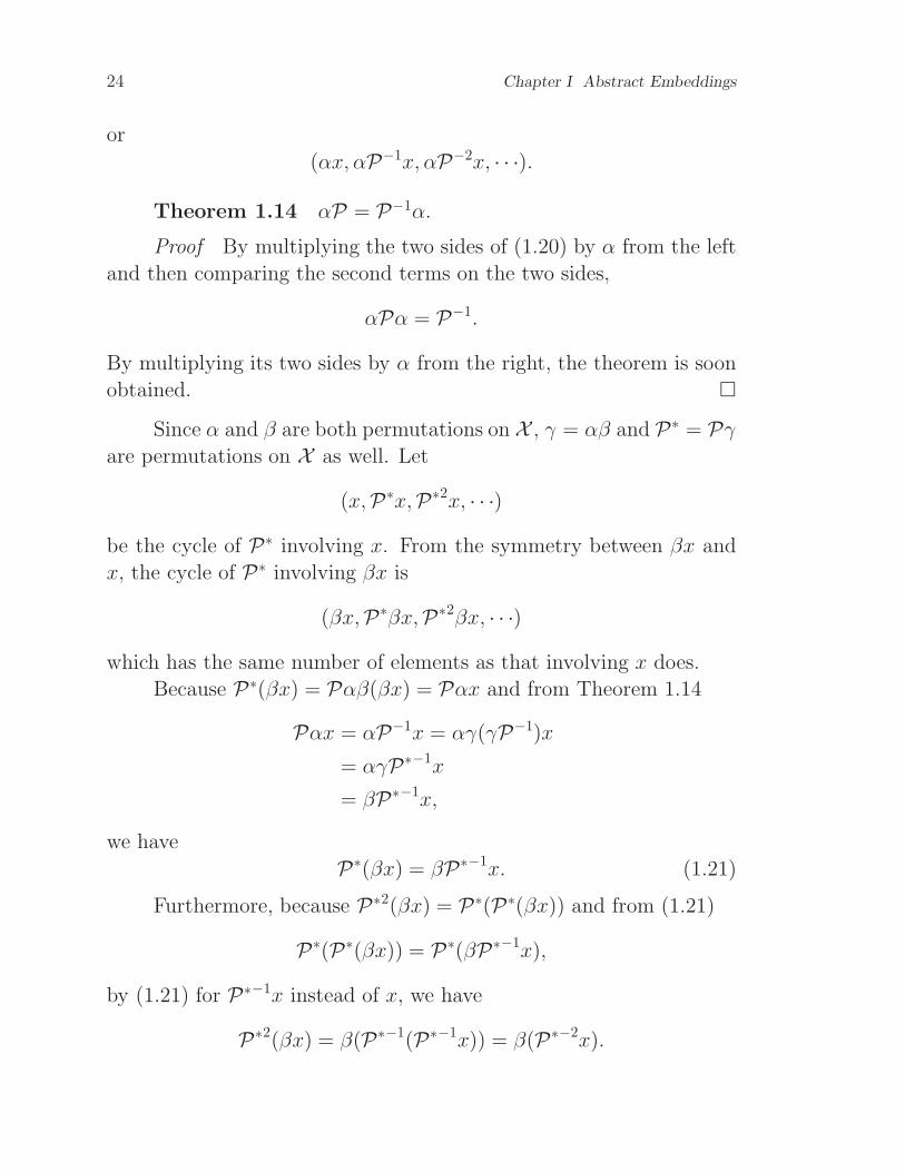
Theorem 1.14 αP = P−1α.
Proof By multiplying the two sides of (1.20) by α from the left
and then comparing the second terms on the two sides,
αPα = P−1.
By multiplying its two sides by α from the right, the theorem is soon
obtained.
Since α and β are both permutations on X , γ = αβ and P∗ = Pγare permutations on X as well. Let
(x,P∗x,P∗2x, · · ·)
be the cycle of P∗ involving x. From the symmetry between βx and
x, the cycle of P∗ involving βx is
(βx,P∗βx,P∗2βx, · · ·)
which has the same number of elements as that involving x does.
Because P∗(βx) = Pαβ(βx) = Pαx and from Theorem 1.14
Pαx = αP−1x = αγ(γP−1)x
= αγP∗−1x
= βP∗−1x,
we have
P∗(βx) = βP∗−1x. (1.21)
Furthermore, because P∗2(βx) = P∗(P∗(βx)) and from (1.21)
P∗(P∗(βx)) = P∗(βP∗−1x),
by (1.21) for P∗−1x instead of x, we have
P∗2(βx) = β(P∗−1(P∗−1x)) = β(P∗−2x).

I.4 Abstract representation 25
On the basis of the finite restrict recursion principle, a cycle is found.
Therefore,
(βx,P∗βx,P∗2βx, · · ·) = β(x,P∗−1x,P∗−2x, · · ·). (1.22)
This implies
(x)P∗
⋂(βx)P∗ = ∅, (1.23)
for x ∈ X .
Theorem 1.15 βP∗ = P∗−1β.
Proof A direct result of (1.22).
Based on (1.22), it is seen that the face involving x of the em-
bedding represented by P is
(x,P∗x,P∗2x, · · ·), (βx,P∗−1βx,P∗−2βx, · · ·). (1.24)
Similarly to vertices, based on (1.22) and (1.23), the face can be
represented by one of the two cycles in (1.24).
Example 1.3 Let G = K4, i.e. , the complete set of order 4.
Given its rotation
(x, y, z), (βz, l, γw), (γl, u, βy), (βx, w, γu),as shown in Fig 1.12. Its two faces are (x, βu, βl, γz) and
(y, αu, αw, αl, γy, z, βw, γx).
-w x ?y Rz
Iu l
v4
v1
v2
v3
Fig.1.12 A rotation of K4

26 Chapter I Abstract Embeddings
Thus, it is an embedding of K4 on the torus
O1 = (ABA−1B−1)
as shown in Fig.1.13.
wA A
αx
6y B6
B
Rαz
Iαu
αl
v4
v1
v2
v3
Fig.1.13 Embedding determined by rotation
Further, another rotation of K4 is chosen for getting another
embedding of K4.
Example 1.4(Continuous to Example 1.3) Another embedding
of K4 is shown as in Fig.1.14. Its rotation is
(x, y, z), (βz, l, γw), (u, γy, γl), (βx,w, γu).
Its two faces are
(x, βu, βl, γz)
and
(αx, w, βz, αy, αu, αw, αl, βy).
This is an embedding of K4 on the Klein bottle
N2 = (ABA−1B) ∼top= (AABB)

I.5 Smarandache 2-manifolds with map geometry 27
as shown in Fig.1.14.
wA A
αx
6y B6
B ?βy
Rαz
Iαu
αl
v4
v1
v2
v3
Fig.1.14 Embedding distinguished by rotation
Such an idea is preferable to deal with combinatorial maps via
algebraic but neither geometric nor topological approaches.
I.5 Smarandache 2-manifolds with map geometry
Smarandache system The embedding of a graph on surface
enables one to construct finitely Smarandache 2-manifolds, i.e., map
geometries on surfaces.
A rule in a mathematical system (Σ;R) is said to be Smaran-
dachely denied if it behaves in at least two different ways within the
same set Σ, i.e., validated and invalided, or only invalided but in mul-
tiple distinct ways.
A Smarandache system (Σ;R) is a mathematical system which
has at least one Smarandachely denied rule in R (see [Mao4] for de-
tails). Particularly, if (Σ;R) is nothing but a metric space (M ; ρ),
then such a Smarandache system is called a Smarandache geometry,
seeing references [Mao1]–[Mao4] and [Sma1]–[Sma2].
Example 1.5(Smarandache geometry) Let R2 be a Euclidean
plane, points A,B ∈ R2 and l a straight line, where each straight

28 Chapter I Abstract Embeddings
line passes through A will turn 30o degree to the upper and passes
through B will turn 30o degree to the down such as those shown in
Fig.1.15. Then each line passing through A in F1 will intersect with
l, lines passing through B in F2 will not intersect with l and there is
only one line passing through other points does not intersect with l.-- A
B
l
30o
30o
30o
30o
..............
...........
..................
..............
...........
........
..........
.............
F1
F2
Fig.1.15
Then such a geometry space R2 with queer points A and B is
a Smarandache geometry since the axiom given a line and a point
exterior this line, there is one line parallel to this line is now replaced
by none line, one line and infinite lines.
A more general way for constructing Smarandache geometries
is by Smarandache multi-spaces ([Mao3]). For an integer m ≥ 2, let
(Σ1;R1), (Σ2;R2), · · ·, (Σm;Rm) be m mathematical systems different
two by two. A Smarandache multi-space is a pair (Σ; R) with
Σ =m⋃
i=1
Σi, and R =m⋃
i=1
Ri.
Such a multi-space naturally induce a graph structure with
V (G) = Σ1,Σ2, · · · ,Σm,E(G) = (Σi,Σj) | Σi
⋂Σj 6= ∅, 1 ≤ i, j ≤ m.
Example 1.16([Mao5]) Let n be an integer, Z1 = (0, 1, 2, · · · , n−1,+) an additive group (modn) and P = (0, 1, 2, · · · , n− 1) a permu-
tation. For any integer i, 0 ≤ i ≤ n− 1, define
Zi+1 = P i(Z1)
such that P i(k) +i Pi(l) = P i(m) in Zi+1 if k+ l = m in Z1, where +i

I.5 Smarandache 2-manifolds with map geometry 29
denotes the binary operation +i : (P i(k), P i(l)) → P i(m). Then we
know that
(n⋃
i=1
Zi;O
)
withO = +i, 0 ≤ i ≤ n−1 is a Smarandache multi-space underlying
a graph Kn, where Zi = Z1 for integers 1 ≤ i ≤ n.
Map geometry A nice model on Smarandache geometries,
namely s-manifolds on the plane was found by Iseri in [Ise1] defined
as follows, which is in fact a case of map geometry.
An s-manifold is any collection C(T, n) of these equilateral trian-
gular disks Ti, 1 ≤ i ≤ n satisfying the following conditions:
(i) each edge e is the identification of at most two edges ei, ej in
two distinct triangular disks Ti, Tj, 1 ≤ i, j ≤ n and i 6= j;
(ii) each vertex v is the identification of one vertex in each of
five, six or seven distinct triangular disks.
These vertices are classified by the number of the disks around
them. A vertex around five, six or seven triangular disks is called an
elliptic vertex, an Euclidean vertex or a hyperbolic vertex, respectively.
* jA A
O
L1 * *P
L2
63B B
Q
Q
L3
(a) (b) (c)
Fig.1.16
In a plane, an elliptic vertex O, a Euclidean vertex P and a
hyperbolic vertex Q and an s-line L1, L2 or L3 passes through points
O, P or Q are shown in Fig.1.16(a), (b), (c), respectively.
The map geometry is gotten by endowing an angular function
µ : V (M)→ [0, 4π) on an embedding M for generalizing Iseri’s model

30 Chapter I Abstract Embeddings
on surfaces following, which was first introduced in [Mao2].
Map geometry without boundary Let M be a combinato-
rial map on a surface S with each vertex valency≥ 3 and µ : V (M)→[0, 4π), i.e., endow each vertex u, u ∈ V (M) with a real number µ(u), 0 <
µ(u) < 4πρM (u)
. The pair (M,µ) is called a map geometry without bound-
ary, µ(u) an angle factor on u and orientable or non-orientable if M
is orientable or not.
Map geometry with boundary Let (M,µ) be a map geom-
etry without boundary, faces f1, f2, · · · , fl ∈ F (M), 1 ≤ l ≤ φ(M) −1. If S(M) \ f1, f2, · · · , fl is connected, then (M,µ)−l = (S(M) \f1, f2, · · · , fl, µ) is called a map geometry with boundary f1, f2, · · · , fl,
and orientable or not if (M,µ) is orientable or not, where S(M) de-
notes the underlying surface of M .
u
u
u
ρM (u)µ(u) < 2π ρM (u)µ(u) = 2π ρM (u)µ(u) > 2π
Fig.1.17
Certainly, a vertex u ∈ V (M) with ρM(u)µ(u) < 2π, = 2π or
> 2π can be also realized in a Euclidean space R3, such as those
shown in Fig.1.17.
A point u in a map geometry (M,µ) is said to be elliptic, Eu-
clidean or hyperbolic if ρM(u)µ(u) < 2π, ρM (u)µ(u) = 2π or ρM(u)µ(u) >
2π. If µ(u) = 60o, we find these elliptic, Euclidean or hyperbolic ver-
tices are just the same in Iseri’s model, which means that these s-
manifolds are a special map geometry. If a line passes through a point
u, it must has an angle ρM (u)µ(u)2 with the entering ray and equal to
180o only when u is Euclidean. For convenience, we always assume
that a line passing through an elliptic point turn to the left and a hy-
perbolic point to the right on the plane. Then we know the following

I.5 Smarandache 2-manifolds with map geometry 31
results.
Theorem 1.16 Let M be an embedding on a locally orientable
surface with |M | ≥ 3 and ρM(u) ≥ 3 for ∀u ∈ V (M). Then there exists
an angle factor µ : V (M)→ [0, 4π) such that (M,µ) is a Smarandache
geometry by denial the axiom (E5) with axioms (E5) for Euclidean,
(L5) for hyperbolic and (R5) for elliptic.
Theorem 1.17 Let M be an embedding on a locally orientable
surface with order≥ 3, vertex valency≥ 3 and a face f ∈ F (M). Then
there is an angle factor µ : V (M) → [0, 4π) such that (M,µ)−1 is a
Smarandache geometry by denial the axiom (E5) with axioms (E5)
for Euclidean, (L5) for hyperbolic and (R5) for elliptic.
A complete proof of Theorems 1.16–1.17 can be found in refer-
ences in [Mao2–4]. It should be noted that the map geometry with
boundary is in fact a generalization of Klein model for hyperbolic
geometry, which uses a boundary circle and lines are straight line seg-
ment in this circle, such as those shown in Fig.1.18.
L1
L2
L3
Fig.1.18

Activities on Chapter I
I.6 Observations
O1.1 Let X be a finite set and B be a binary set. Is Bx|x ∈X a pregraph or a graph? If unnecessary, what condition does a
pregraph, or a graph satisfy?
O1.2 Let X be a finite set, B be a binary set and
X =∑
x∈XBx.
For a permutation ψ on X such that ψ2 = 1, is x, ψx|x ∈ X a
graph? If unnecessary, when is it a graph?
O1.3 How many orientable, or nonorientable surfaces can a
hexagon represent? List all of them.
O1.4 How many orientable, or nonorientable surfaces can a 2k-
gon represent? How to List them all.
O1.5 In [Liu1], an embedding of a graph G on the nonori-
entable surface of genus β(G) is constructed in a way from a specific
tree on G. Now, how to get such an embedding from any tree on G.
O1.6 Suppose G has an embedding on an orientable surface
of genus k. If k is not the maximum genus of G, how to find an
embedding of G on an orientable surface of genus k + 1.
O1.7 Any embedding of a graph G = (V,X) is a permutation
on 1, α, β, αβX = X as shown by (1.17). However, α, β and γ = αβ
are each a permutation on X , but not an embedding of G in general.
When does each of them determine an embedding of G.

I.6 Observations 33
O1.8 If permutation P on X is an embedding of a graph, to
show that for any x ∈ X , there does not exist an integer m such that
αx = Pmx.
O1.9 If permutation P on X is an embedding of a graph, to
show
PαP = α.
O1.10 Observe that permutation β as P satisfies both O1.8
and O1.9. However, permutation α as P satisfies O1.9 but not O1.8.
O1.11 Let S be a set of permutations on X and ΨS be the
group generated by S. If for any x, y ∈ X , there exists a ψ ∈ ΨS such
that x = ψy, then the group ΨS is said to be transitive on X . Observe
that if permutation P on X is an embedding of a graph, then group
ΨI , I = P , α, β, is transitive on X .
An embedding of a graph G = (V,E) can be combinatorially
represented by a rotation system σ(V ) on the vertex set V of G and
a function on the edge set as λ : E −→ B, B = 0, 1, denoted by
Gσ(λ).
In order to determine the faces of an embedding, an immersion
of the graph and a rule should be established.
An immersion of a graph is such a representation of the graph in
the plane that vertices injects into the plane on an imaged circle and
edges are straight line segments between their two ends.
Travel and traverse rule From a point on one side of an edge,
travel as long as on the same side until at the middle of a edge with
λ = 1, then traverse to the other side.
O1.12 By the TT-rule(i.e., the travel and traverse rule) on
an immersion, the initial side the starting point is on can always be
encountered to get a travel as a set of edges met on the way.
O1.13 By the TT-rule on an immersion of a graph, a set of
travels can always be found for any edge occurs exactly twice.

34 Activities on Chapter I
On a graph G = (V,E), a subset of edges C ⊆ E that V has a
2-partition V = V1 + V2 with the property:
C = (u, v) ∈ E|u ∈ V1, v ∈ V2 (1.25)
is called a cocycle of G.
O1.14 For an immersion Gσ(λ) of graph G = (V,E), the em-
bedding of G determined by Gσ(λ) is orientable if, and only if, the set
e|∀e ∈ E,≤ (e) = 1 is a cocycle of G.
I.7 Exercises
E1.1 For a graph G, prove that G has no odd circuit(a circuit
with odd number of edges) if, and only if, for a tree on G, G has no
odd fundamental circuit.
E1.2 Prove that a graph G = (V,E) has no odd fundamental
circuit if, and only if, E itself is a cocycle.
Let Γ be a nonAbelian group. The identity is denoted by 1.
Write Γ0 = ξ|ξ2 = 1, ξ ∈ Γ, i.e., the set of all elements of order 2.
For a pregraph G = (V,E), let xv ∈ Γ0, v ∈ V , be variables on the
vertex set V and w(e) ∈ Γ0, e ∈ E be a weight function on the edge
set E. On the network N = (G;w), its incidence equation is
xuxv = w(e), e ∈ E. (1.26)
E1.3 Prove that if the incidence equation has a solution, then
it has at least |Γ0|, i.e. , the number of elements in Γ0, solutions.
E1.4 Prove that the incidence equation has a solution if, and
only if, G has no circuit C such that
w(C) =∏
e∈Cw(e) 6= 1.
E1.5 Let σ(G) be the number of connected components on pre-
graph G. Prove that if the incidence equation has a solution, then it

I.7 Exercises 35
has
|Γ0|σ(G)
solutions.
E1.6 For an orientable surface, provide a procedure for deter-
mining its orientable genus and then estimate an upper bound of the
operations necessary.
E1.7 For a nonorientable surface, provide a procedure for de-
termining its nonorientable genus and then estimate an upper bound
of the number of operations necessarily used.
E1.8 Let G be a graph of order 2 with all its edges selfloops but
only one. Prove that G is not up-embeddable on orientable surfaces
if, and only if, each vertex is incident with odd number of selfloops.
E1.9 According to the orientable and nonorientable genera, list
all embeddings of K4, the complete graph of order 4.
A graph is called i-separable if it has i, i ≥ 1, vertices such that
it is not connected anymore when the i vertices with their incident
edges are deleted. A set of i vertices separable without a proper subset
separable for a graph is called an i-cut of the graph. A graph which
has an i-cut without (i− 1)-cut is said to be i-connected.
E1.10 Prove that if a 3-connected graph G is planar (embed-
dable on the sphere), then it has exact 2 embeddings on the sphere.
For a planar graph G = (V,E), and u, v ∈ V , if G has the form
as
G =
G1
⋃G2, (u, v) ∈ E;
G1
⋃G2 − (u, v), (u, v) 6∈ E
(1.27)
and
G1
⋂G2 = (u, v) (1.28)
such that G1 and G2 are both with at least 2 edges, then u, v is
called a splitting pair of G, and G1 and G2, its splitting block. If a
splitting block at a splitting pair has no proper subgraph is still a
splitting block, then it is said to be standard[Mac1].

36 Activities on Chapter I
E1.11 Prove the following three statements.
(i) Let A and B be two standard splitting blocks of a splitting
pair, then they are no edge in common;
(ii) For a splitting pair of a 2-connected planar graphG = (V,E),
the standard splitting block decomposition of the edge set E, i.e.,
E = E1
⋃E2
⋃· · ·⋃Es
such that Ei ∩ Ej = ∅, 1 ≤ i 6= j ≤ s, and the induced subgraphs of
Ei, 1 ≤ i ≤ s, are all standard splitting blocks of the splitting pair, is
unique.
(iii) Let bi be the number of standard splitting blocks of the
ith splitting pair, i = 1, 2, · · · , m, m be the number of splitting pairs,
then the number of embeddings of a 2-connected planar graph on the
sphere is
2b1+b2+···+bm
m∏
i=1
(bi − 1)!.
For a graph G, let Π(G) be the set of rotation systems of inner
vertices on a joint tree and ωπ(i), π ∈ Π, be the boundary polygon
with its β(G) pairs of letters whose indices are determined by a binary
number i with β(G) digits by the rule: the two indices of the lth letter
are same or different according as the lth digit of i is 0 or 1. Define
ξ(ωπ(i)) =
⌊β(G)2 ⌋∑
k=−β(G)
akxk (1.29)
where x is an undeterminate and
ak =
1, if ωπ(i) ∼top Ok, or Q−k;
0, otherwise.(1.30)
Now, let
Ωπ = ωπ(i)| 0 ≤ i ≤ 2β(G) − 1 (1.31)
and
ξ(Ωπ) =
2β(G)−1∑
i=0
ξ(ωπ(i)). (1.32)

I.8 Researches 37
E1.12 Prove that the coefficient of xk in
ξ(G) =∑
π∈Π(G)
ξ(Ωπ)
is the number of embeddings of G on the surface of relative genus k,
−β(G) ≤ k ≤ ⌊β(G)2 ⌋.
A graph of order 2 without selfloop is called a link bundle.
E1.13 Let Lm be the link bundle of size m ≥ 1. Determine
ξ(Lm).
A graph of order 1 is also called a bouquet, or a loop bundle.
E1.14 Let Bm be a bouquet of size m, m ≥ 1. Determine
ξ(Bm).
A graph of order 2 is called a bipole. Of course, a link bundle is
a bipole which has no selfloop.
E1.15 Let Pm be a bipole of size m, m ≥ 1. Determine ξ(Pm).
I.8 Researches
The set(repetition at most twice of elements permitted) of edges
appearing on a travel can be shown to have a partition of each subset
forming still a subtravel except probably the travel itself. Such a
partition is called a decomposition of a travel into subtravels. However,
it is not yet known if any travel can be decomposed into tours except
only the case that its induced graph has a cut-edge.
R1.1 Prove, or disprove, the conjecture that a travel with at
most twice occurrences of an edge in a graph has a decomposition
into tours if, and only if, the induced subgraph of the travel is without
cut-edge.
Because a circuit is restricted from a tour by no repetition of a
vertex, the following conjecture would look stronger the last one.
R1.2 Prove, or disprove, the conjecture that a travel with at

38 Activities on Chapter I
most twice occurrences of an edge in a graph has a decomposition into
circuits if, and only if, the induced subgraph of the travel is without
cut-edge.
However, it can be shown from Theorem 1.3 that any tour has
a decomposition into circuits. The above two conjectures are, in fact,
equivalent. Because a cut-edge is never on a circuit, the necessity
is always true. A travel with three occurrences of an edge permitted
does not have a decomposition into circuits in general. For example, on
the graph determined by Par= x(0), y(0), x(1), y(1), the travel
xx−1xy−1 where x = 〈x(0), x(1)〉 and y = 〈y(0), y(1)〉 has no circuit
decomposition.
Furthermore, the two conjectures are apparently right when the
graph is planar because each face boundary of its planar embedding
is generally a tour whenever without cut-edge.
R1.3 For a given graph G and an integer p, p ≥ 0, find the
number np(G) of embeddings of G on the orientable surface of genus
p.
The aim is at the genus distribution of embeddings of G on ori-
entable surfaces, i.e., the polynomial
PO(G) =
⌊σ/2⌋∑
p=0
np(G)xp,
where σ is the Betti number of G.
For p = 0, n0(G) can be done based on [Liu6]. If G is planar,
O1.11 provides the result for 2-connected case. Others can also be
derived. As to justify if a graph is planar, a theory can be seen from
Chapters 3,5 and 7 in [Liu5].
Generally speaking, not easy to get the complete answer in a
short period of time. However, the following approach would be avail-
able to access this problem. Choose a special type of graphs, for
instance, a wheel(a circuit Cn all of whose vertices are adjacent to an
extra vertex), a generalized Halin graph(a circuit with a disjoint tree

I.8 Researches 39
except for all articulate vertices forming the vertex set of the circuit)
and so forth.
Of course, the technique and theoretical results in 1.3 can be
employed to calculate the number of distinct embeddings of a graph
by hand and by computer.
R1.4 Orientable single peak conjecture. The coefficients of the
polynomial in R1.3 are of single peak , i.e., they are from increase to
decrease as p runs from 0 to ⌊σ/2⌋(≥ 3), np(G).
The purpose here is to prove, or disprove the conjecture not nec-
essary to get all np(G), 0 ≤ p ≤ ⌊σ/2⌋(≥ 3).
R1.5 Determine the number of distinct embeddings, which have
one, or two faces, of a graph on orientable surfaces.
R1.6 For a given graphG and an integer q, q ≥ 1, find the num-
ber nq(G) of distinct embeddings on nonorientable surfaces of genus
q.
The aim is at the genus polynomial of embeddings ofG on nonori-
entable surfaces:
PN(G) =σ∑
q=1
nq(G)xq,
where σ is the Betti number of G.
Some pre-investigations for G is that a wheel, or a generalized
Halin graph can firstly be done.
R1.7 For a graphG, justify if it is embeddable on the projective
plane, and then determine n1(G) according to the connectivity of G.
R1.8 For a graph embeddable on the projective plane, determine
how many sets of circuits such that for each, all of its circuits are
essential if, and only if, one of them is essential in an embedding of G
on the projective plane.
R1.9 Nonorientable single peak conjecture. The coefficients of
the polynomial in R1.6 are of single peak in the interval [o, σ] where
σ is the Betti number of G.

40 Activities on Chapter I
R1.10 For a given type of graphs G and an integer p, find the
number of distinct embeddings of graphs in G on the orientable surface
of genus p. Further, determine the polynomial
PO(G) =
⌊σ(G)/2⌋∑
p=0
np(G)xp
where σ(G) = maxσ(G)|G ∈ G.R1.11 For a given type of graphs G and an integer q, q ≥ 1,
find the number of embeddings of graphs in G on the nonorientable
surface of genus q. Further, determine the polynomial
PN (G) =
σ(G)∑
q=1
nq(G)xq
where σ(G) = maxσ(G)|G ∈ G.R1.12 For a set of graphs with some fixed invariants, extract
sharp bounds(lower or upper) of the orientable minimum genus and
sharp bounds(lower or upper) of orientable maximum genus.
Here, invariants are chosen from the order (vertex number), size(edge
number), chromatic number (the minimum number of colors by which
vertices of a graph can be colored such that adjacent vertices have
distinct colors), crossing number(the minimum number of crossing in-
ner points among all planar immersions of a graph), thickness (the
minimum number of subsets among all partitions of the edge set such
that each of the subsets induces a planar graph), and so forth.
R1.13 For a set of graphs and a set of invariants fixed, pro-
vide sharp bounds(lower or upper) of minimum nonorientable genus
of embeddings of graphs in the set.

Chapter II
Abstract Maps
• A ground set is formed by the Klein group K = 1, α, β, αβ stick-
ing on a finite set X.
• A basic permutation is such a permutation on the ground set that
no element x is in the same cycle with αx.
• The conjugate axiom on a map is determined by each vertex con-
sisting of two conjugate cycles for α, as well as by each face con-
sisting of two conjugate cycles for β.
• The transitive axiom on a map is from the connectedness of its
underlying graph.
• An included angle is determined by either a vertex with one of its
incident faces, or a face with one of its incident vertices.
II.1 Ground sets
Given a finite set X = x1, x2, · · · , xm, called the basic set, its
elements are distinct. Two operations α and β on X are defined
as for any x ∈ X, αx 6= βx, αx, βx 6∈ X and α2x = α(αx) = x,
β2x = β(βx) = x. Further, define αβ = βα = γ such that for any
x ∈ X, γx 6= αx, βx and γx 6∈ X.

42 Chapter II Abstract Maps
Let αX = αx|∀x ∈ X, βX = βx|∀x ∈ X and γX =
γx|∀x ∈ X, then α, β and γ determine a bijection between X and,
respectively, αX, βX and γX. By a bijection is meant a one to one
correspondence between two sets of the same cardinality. In other
words,
X⋂
αX = X⋂
βX = X⋂
γX = ∅;αX
⋂βX = βX
⋂γX = γX
⋂αX = ∅;
|αX| = |βX| = |γX| = |X|.(2.1)
The set X∪αX ∪βX∪γX, or briefly X = X (X), is called the ground
set.
Now, observe set K = 1, α, β, γ. Its elements are seen as
permutations on the ground set X . Here, 1 is the identity. From
α2 = β2 = 1 and αβ = βα, γ2 = (αβ)(αβ) = α(ββ)α = α2 = 1, and
hence
α =m∏
i=1
(xi, αxi)m∏
i=1
(βxi, γxi);
β =m∏
i=1
(xi, βxi)m∏
i=1
(αxi, γxi);
γ =
m∏
i=1
(xi, γxi)
m∏
i=1
(βxi, αxi).
(2.2)
It is easily seen that K is a group, called Klein group because it is
isomorphic to the group of four elements discovered by Klein in geom-
etry.
For any x ∈ X , let Kx = x, αx, βx, γx, called a quadricell.
Theorem 2.1 For any basic set X, its ground set is
X =∑
x∈XKx, (2.3)
where the summation represents the disjoint union of sets.
Proof From (2.1), for any x, y ∈ X and x 6= y,
Kx⋂Ky = x, αxβx, γx
⋂y, αy, βy, γy = ∅.

II.2 Basic permutations 43
From (2.1) again,
⋃
x∈XKx = X + αX + βX + γX = X .
Therefore, (2.3) is true.
Furthermore, since for any x ∈ X,
K(αx) = K(βx) = K(γx) = Kx, (2.4)
we have
X =∑
y∈αX
Ky =∑
z∈βX
Kz =∑
t∈γX
Kt.
This implies that the four elements in a quadricell are with symmetry.
II.2 Basic permutations
Let Per(X ), or briefly Per, be a permutation on the ground set X .
Because of bijection, according to the finite strict recursion principle,
for any x ∈ X , there exists a minimum positive integer k(x) such that
Perk(x)x = x,
i.e., Per contains the cyclic permutation , or in short cycle,
(x)Per = (x,Per2x, · · · ,Perk(x)−1x).
Write xPer as the set of all elements in the cycle (x)Per. Such a set is
called the orbit of x under permutation Per. The integer k(x) is called
the order of x under permutation Per.
If for any x ∈ X ,
αx 6∈ xPer, (2.5)
then the permutation Per is said to be basic to α.
Example 2.1 From (2.2), for permutations α and β on the
ground set, α is not basic, but β is basic.

44 Chapter II Abstract Maps
Let Par= X1, X2, · · · , Xs be a partition on the ground set X ,
then
Per =
s∏
i=1
(Xi) (2.6)
determines a permutation on X , called induced from the partition Par.
Here, (Xi), 1 ≤ i ≤ s, stands for a cyclic order arranged on Xi. This
shows that a partition Xi|1 ≤ i ≤ s has
s∏
s=1
(|Xi| − 1)! =∏
i≥3
((i− 1)!)ni (2.7)
induced permutations. In (2.7), ni, i ≥ 3, is the number of subsets in
Par with i elements.
Theorem 2.2 Let Par= Xi|1 ≤ i ≤ s be a partition on the
ground set X (X). If Par has an induced permutation basic, then all
of its induced permutations are basic. Further, a partition Par has its
induced permutation basic if, and only if, for x ∈ X , there does not
exist Y ∈ Par such that
x, αx or βx, γx ⊆ Y⋂
Kx. (2.8)
Proof Because the basicness of a permutation is independent of
the order on cycles, the first statement is proved.
Assume an induced permutation Per of a partition Par is basic.
From (2.5), for any x ∈ X, in virtue of
Kx = x, αx+ βx, γx,no Y ∈Par exists such that (2.8) is satisfied. This is the necessity of
the second statement.
Conversely, because for any x ∈ X , no Y ∈ Par exists such that
(2.8) is satisfied, it is only possible that x and αx are in distinct subsets
of partition Par. Therefore, αx 6∈ xPer. Based on (2.5), this is the
sufficiency of the second statement.
On the basis of this theorem, induced basic permutations can be
easily extracted from a partition of the ground set.

II.2 Basic permutations 45
Example 2.2 Let X = x, αx, βx, γx = Kx. There are 15
partitions on X as
Par1 = x, αx, βx, γx;Par2 = x, αx, βx, γx;Par3 = x, βx, αx, γx;Par4 = x, γx, αx, βx;Par5 = βx, αx, x, γx;Par6 = x, αx, γx, βx;Par7 = x, αx, βx, γx;Par8 = x, αx, βx, γx;Par9 = x, βx, γx, βx;Par10 = x, αx, γx, αx;Par11 = x, αx, βx, γx;Par12 = x, αx, βx, γx;Par13 = x, αx, βx, γx;Par14 = x, βx, αx, γx;Par15 = x, γx, αx, βx.
From Theorem 2.2, induced basic permutations can only be extracted
from Par1, Par3, Par4, Par5, Par6, Par14 and Par15 among them. Since
each of these partitions has no subset with at least 3 elements, from
(2.7) it only induces 1 basic permutation. Hence, 7 basic permutations
are induced in all.
Based on Theorem 2.2, a partition that induces a basic permu-
tation is called basic as well.
For a partition Par on X , if every pair of x and αx, x ∈ X , deals
with the element x in Par, then this partition determines a pregraph
if any. For example, in Example 2, there are only
Par1 = Par2 = Par7 = Par13 = x, βx;Par12 = Par14 = Par15 = x, βx
form 2 premaps of size 1 and others meaningless among the 15 par-

46 Chapter II Abstract Maps
titions. Further, each of the 2 premaps is a graph. The result is the
same as in Example 1.1.
II.3 Conjugate axiom
Let Per1 and Per2 be two permutations on the ground set X . If
for x ∈ X ,
(Per2x)Per1= Per2(x)Per
−1
1
= Per2(x)−1
Per1, (2.9)
then the two orbits (x)Per1 and (Per2x)Per1 of Per1 are said to be con-
jugate.
For a permutation P on the ground set X , if
αP = P−1α, (2.10)
then (P , α)(or for the sake of brevity, P) is called satisfying the con-
jugate axiom.
Theorem 2.3 For a basic permutation P on the ground set X ,
the two orbits (x)P and (αx)P for any x ∈ X are conjugate if, and
only if, (P , α) satisfies the conjugate axiom.
Proof Necessity. Because of orbits (x)P and (αx)P conjugate,
from (2.9), (αx)P = α(x)−1P . Hence, Pαx = αP−1x, i.e., Pα = αP−1.
This implies (2.10).
Sufficiency. Since P satisfies (2.10),
P(αx) = P(αP)P−1x = P(P−1α)P−1x
= (PP−1)αP−1x = αP−1x.
By induction, assume that P l(αx) = αP−lx, l ≥ 1, then we have
P l+1(αx) = PP l(αx) = PP−lx
= P(αPP−1)P−lx ( then by (2.10))
= (PP−1)αP−(l+1)x
= αP−(l+1)x.

II.3 Conjugate axiom 47
Hence, (αx)P = α(x)−1P . From (2.9), orbits (x)P and (αx)P are conju-
gate. This is the sufficiency.
Unlike Theorem 2.2, for a partition on the ground set X , from
one of its induced permutations satisfying the conjugate axiom, it can
not be deduced to others.
A premap, denoted by (Xα,β,P), is such a basic permutation Pon the ground set X that the conjugate axiom is satisfied for (P , α).
Example 2.3 By no means any basic partition is in companion
with a basic permutation. Among the 7 basic partitions as shown in
Example 2.2, only the induced permutations of Par1, Par14 and Par15
are premaps.
Because (P , β) is not necessary to satisfy the conjugate axiom
on a premap (X ,P), α is called the first operation and β, the second
. Thus, X should be precisely written as Xα,β if necessary.
Based on the basicness and Theorem 2.3, any premap P has the
form as ∏
x∈XP
(x)P(x)∗P, (2.11)
where XP is the set of distinct representatives for the conjugate pairs
xP , x∗P of cycles in P . And further,
X =∑
x∈XP
xPx∗P . (2.12)
For convenience, one of two conjugate orbits in xP , x∗P is chosen
to stand for the pair itself as a vertex of the premap.
Example 2.4 Let X = x1, x2, then
X = x1, αx1, βx1, γx1, x2, αx2, βx2, γx2.Choose
P1 = (x1, βx1)(αx1, γx1)(x2)(αx2)(βx2)(γx2)
and
P2 = (x1, βx1, x2)(αx1, αx2, γx1)(βx2)(γx2).

48 Chapter II Abstract Maps
The former has 3 vertices (x1, βx1), (x2) and (βx2). The latter has 2
vertices (x1, βx1, x2) and (βx2).
Lemma 2.1 If permutation P on Xα,β is a premap, then
P∗β = βP∗−1, (2.13)
where P∗ = Pγ, γ = αβ.
Proof Because P∗β = Pαββ = Pα, from the conjugate axiom,
P∗β = αP−1
= ββαP−1 ( β2 = 1)
= β((Pαβ)−1)
= βP∗−1.
Therefore, the lemma holds.
This lemma tells us that although β does not satisfy the conju-
gate axiom for permutation P in general, β does satisfy the conjugate
axiom for permutation P∗.
Lemma 2.2 If permutation P on Xα,β is a premap, then per-
mutation P∗ = Pγ is basic for β.
Proof Because the 4 elements in a quadricell are distinct, x 6=βx.
Case 1 P∗x 6= βx. Otherwise, from P∗x = βx, Pα(βx) =
P∗x = βx. A contradiction to that P is basic for α.
Case 2 (P∗)2x 6= βx. Otherwise, P∗x = P∗−1βx. From Lemma
2.1, P∗x = βP∗x. A contradiction to that P∗x and βP∗x are in the
same quadricell.
In general, assume by induction that Case l: (P∗)lx 6= βx, 1 ≤l ≤ k, k ≥ 2, is proved. To prove
Case k + 1 (P∗)k+1x 6= βx. Otherwise, P∗kx = P∗−1βx. From
Lemma 2.1, P∗k−1(P∗x) = β(P∗x). A contradiction to the induction
hypothesis.

II.4 Transitive axiom 49
In all, the lemma is proved.
Theorem 2.4 Permutation P on X is a premap (Xα,β,P) if,
and only if, permutation P∗ = Pγ is a premap (Xβ,α,P∗).Proof Necessity. Since permutation P is a premap (Xα,β,P),
P is basic for α and satisfies the conjugate axiom. From Lemma 2.2
and Lemma 2.1, P∗ is basic for β and satisfies the conjugate axiom.
Hence, P∗ is a premap (Xβ,α,P∗).Sufficiency. Because P∗∗ = P∗γ = P , the sufficiency is right.
On the basis of Theorem 2.4, the vertices of premap P∗ are de-
fined to be the faces of premap P . The former is called the dual of
the latter. Since P∗∗ = P , the latter is also the dual of the former.
Example 2.5 For the two premaps P1 and P2 as shown in
Example 2.4, we have
P∗1 = (x1, αx1)(βx1, γx1)(x2, γx2)(βx2, αx2)
and
P∗2 = (x1, αx1, x2, γx2)(βx1, αx2, βx2, γx1).
Because P∗1 has 2 vertices (x1, αx1) and (x2, γx2) and P∗2 has 1 vertex
(x1, αx1, x2, γx2), we seen that premaps P1 and P2 have, respectively,
2 faces and 1 face.
II.4 Transitive axiom
For a set of permutations T = τi|1 ≤ i ≤ k, k ≥ 1 on X , let
ΨT = ψ|ψ =s∏
l=1
k∏
j=1
τij(πl)
πl(j), ij(πl) ∈ Z, πl ∈ Π, s ≥ 1, (2.14)
where Z is the set of integers and Π is the set of all permutations on
1, 2, · · · , k, k ≥ 1.

50 Chapter II Abstract Maps
Since all elements in ΨT are permutations on X , they are closed
for composition(or in other word, multiplication) with the associative
law but without the commutative law.
Further, it is seen that a permutation in ΨT if, and only if, its
inverse is in Ψ. The identity is the element in ΨT when all ij(π) = 0,
π ∈ Π in (2.14). Therefore, ΨT is a group in its own right, called the
generated group of T .
Let Ψ be a permutation group on X . If for any x, y ∈ X , there
exists an element ψ ∈ Ψ such that x = ψy, then the group Ψ is said
to be transitive , or in other words, the group Ψ satisfies the transitive
axiom.
Now, consider a binary relation on X , denoted by ∼Ψ, that for
any x, y ∈ X ,
x ∼Ψ y ⇐⇒ ∃ ψ ∈ Ψ, x = ψy. (2.15)
Because the relation ∼Ψ determined by (2.15) for a permutation
group Ψ on X is a equivalence, X is classified into classes as X /∼Ψ.
Theorem 2.5 A permutation group Ψ on X is transitive if, and
only if, for the equivalence ∼Ψ determined by (2.15), |X / ∼Ψ | = 1.
Proof Necessity. From the transitivity, for any x, y ∈ X , there
exists ψ ∈ Ψ such that x = ψy. In view of (2.15), for any x, y ∈ X ,
x ∼Ψ y. Hence, for ∼Ψ, |X / ∼Ψ | = 1.
Sufficiency. Because |X / ∼Ψ | = 1, for any x, y ∈ X , exists
ψ ∈ Ψ such that x = ψy. Therefore, the permutation group Ψ on Xis transitive.
For a premap, the pregraph with the same vertices and edges as
the premap is is called its under pregraph. Conversely, the premap is
a super premap of its under pregraph.
Let (Xα,β,P) be a premap. If permutation group ΨJ , J =
α, β,P, on the ground set Xα,β is transitive, i.e., with the transitive
axiom, then the premap is called a map .
Lemma 2.3 Let M = (Xα,β,P) be a premap. For any x, y ∈

II.4 Transitive axiom 51
Xα,β, exists ψ ∈ ΨJ , J = α, β,P, such that x = ψy if, and only if,
there is a path from the vertex vx x is with to the vertex vy y is with
in the under pregraph of M .
Proof Necessity. In view of (2.14) with the conjugate axiom,
write
ψ = αδ1P l1ασ1βαδ2P l2ασ2β · · ·βαδsP lsασs,
where δi, σi ∈ 0, 1, 1 ≤ i ≤ s, and li ∈ Z, 1 ≤ i ≤ s. Because
αδsP lsασs and αδ1P l1ασ1 are, respectively, acting on vertices vy and vx,
ψ determines a trail from vy to vx of s− 1 edges. Since there is a trail
between two vertices if, and only if, there is a path between them, the
necessity is done.
Sufficiency. let 〈vs, vs−1, · · · , v1〉,vs = vy, v1 = vx, be a path from
vy to vx in the under pregraph of M . Then, there exist δi, σi ∈ 0, 1,1 ≤ i ≤ s, and li ∈ Z, 1 ≤ i ≤ s, such that
ψ = αδ1P l1ασ1β · · · βαδsP lsασs
and x = ψy. From (2.14), the sufficiency is done .
Theorem 2.6 A premap is a map if, and only if, its under
pregraph is a graph.
Proof From the transitive axiom and Lemma 2.3, its under pre-
graph is a graph. This is the necessity.
Conversely, from the connectedness and Lemma 2,3 , the premap
satisfies the transitive axiom and hence its under pregraph is a graph.
This is the sufficiency.
Example 2.6 In Fig.1.2, the pregraph determined by Par7 has
2 super premaps:
P1 = (x1)(αx1)(γx1)(βx1)(x2, γx2)(αx2, βx2)
and
P1 = (x1)(αx1)(γx1)(βx1)(x2, βx2)(αx2, γx2)
as shown in Fig.2.1.

52 Chapter II Abstract Maps
Æx1
γx1 x2
γx2
(γx1)
(x1)
(x2, γx2)
Æx1
γx1 x2
βx2
(γx1)
(x1)
(x2, βx2)
P1 P2
Fig.2.1 Two super premaps
From Theorem 2.6, none of the two super premaps is a map in
Fig.2.1.
However, the pregraph determined by Par12 is a graph in Fig.1.2.
From Theorem 2.6, each of its super premaps is a map as shown in
the following example.
Example 2.7 In Fig.2.2, there are 223! = 24 distinct embed-
dings of the graph determined by Par12 in Fig.1.2. On the associate(or
boundary) polygon of the joint tree, the pair of a letter is defined to be
of distinct powers when x and γx appear; the same power otherwise.
IvRx1
γx1
x2γx2
IvRx1
γx1
γx2x2
IvRx1
x2
γx1γx2
(a) O0 (b) O0 (c) O1
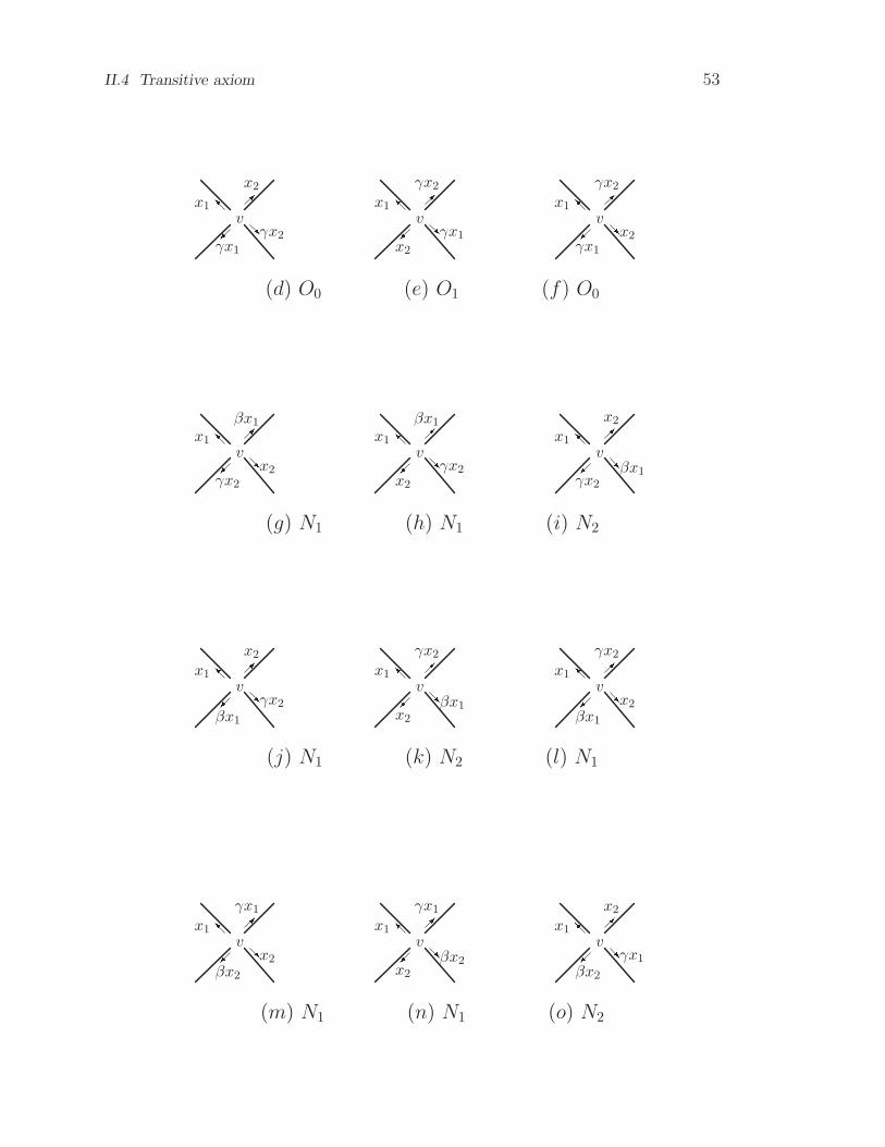
II.4 Transitive axiom 53
IvRx1
x2
γx2γx1
IvRx1
γx2
γx1x2
IvRx1
γx2
x2γx1
(d) O0 (e) O1 (f) O0
IvRx1
βx1
x2γx2
IvRx1
βx1
γx2x2
IvRx1
x2
βx1γx2
(g) N1 (h) N1 (i) N2
IvRx1
x2
γx2βx1
IvRx1
γx2
βx1x2
IvRx1
γx2
x2βx1
(j) N1 (k) N2 (l) N1
IvRx1
γx1
x2βx2
IvRx1
γx1
βx2x2
IvRx1
x2
γx1βx2
(m) N1 (n) N1 (o) N2

54 Chapter II Abstract Maps
IvRx1
x2
βx2γx1
IvRx1
βx2
γx1x2
IvRx1
βx2
x2γx1
(p) N1 (q) N2 (r) N1
IvRx1
βx1
x2βx2
IvRx1
βx1
βx2x2
IvRx1
x2
βx1βx2
(s) N2 (t) N2 (u) N1
IvRx1
x2
βx2βx1
IvRx1
βx2
βx1x2
IvRx1
βx2
x2βx2
(v) N2 (w) N1 (x) N2
Fig.2.2 All embeddings of a graph
In Fig.2.2, the graph determined by Par12(Fig.1.2) has 6 ori-
entable embeddings (a—f). Here, (a), (b), (d) and (f) are the same
map on the sphere O0 ∼top (x1x−11 ). And, (c) and (e) are the same map
on the torus O1 ∼top (x1x2x−11 x−1
2 ). Hence, such 6 distinct embeddings
are, in fact, 2 maps.
Among the 18 nonorientable embeddings, 10 are on the projective
plane and 8 are on the Klein bottle. On the projective plane, (g), (h),
(j), (l), (m), (n), (p) and (r) are the same map (N1 ∼top (x1x−11 x2x2)).

II.5 Included angles 55
And, (u) and (w) are another map (N1 = (x1x2x1x2)). On the Klein
bottle, (i), (k), (o) and (q) are the same map (N2 = (x1x2x−11 x2)).
And, (s), (t), (v) and (x) are another map (N2 ∼top (x1x1x2x2)).
Therefore, there are only 4 maps among the 18 embeddings.
II.5 Included angles
Let M = (Xα,β(X),P) be a premap. Write k = |Xα,β(X)/ ∼ΨJ|,
J = α, β,P, and
Xα,β(X) =k∑
i=1
Xαi,βi(Xi), X =
k∑
i=1
Xi,
where Xαi,βi(X) ∈ Xα,β/ ∼ΨJ
, αi and βi are, respectively, α and β
restricted on Xαi,βi(Xi), i = 1, 2, · · · , k. Further,
M =k∑
i=1
Mi, Mi = (Xαi,βi(Xi),Pi), (2.16)
where Mi is a map and Pi is P restricted on Xαi,βi(Xi), i = 1, 2, · · · , k.
This enables us only to discuss maps without loss of generality.
Lemma 2.4 Any map (X ,P) has that (Pα)2 = 1.
Proof From the conjugate axiom,
(Pα)2 = (Pα)(Pα) = P(αP)α
= (PP−1)(αα) = 1.
This is the conclusion of the lemma.
Lemma 2.5 Any map (X ,P) has that (P∗β)2 = 1.
Proof Because P∗β = Pγβ = Pα(ββ) = Pα, from Lemma 2.4,
the conclusion is obtained.
On the basis of the above two lemmas, on a map M = (Xα,β,P),
any x ∈ Xα,β has that
(x,Pαx) = (P∗βx, x). (2.17)

56 Chapter II Abstract Maps
Thus, 〈x,Pαx〉, or 〈P∗βx, x〉, is called an included angle of the map.
For an edge Kx = x, αx, βx, γx of M , x, αx and βx, γx are its
two ends , or semiedges. And, x, βx and αx, γx are its two sides,
or cosemiedges.
Theorem 2.7 For a (X (X),P), let V = v|v = xP ∪αxP ,∀x ∈ X and F = f |f = xP∗ ∪ βxP∗, ∀x ∈ X. If xv and xf
are, respectively, in v and f as representatives, then
X =∑
v∈V(xv, αP−1xv+ Pxv, αxv+ · · ·
+ P−1xv, αP−2xv)=∑
f∈F(xf , βP∗−1xf+ P∗xf , βxf+ · · ·
+ P∗−1xf , βP∗−2xf).
(2.18)
Proof From X =∑
v∈V v and the conjugate axiom,
v = xv,Pαxv+ Pxv,PαPxv+ · · ·+ P−1xv,PαP−1xv
= xv, αP−1xv+ Pxv, αxv+ · · ·+ P−1xv, αP−2xv.
This is the first equality.
The second equality can similarly be derived from X =∑
f∈F fand Lemma 2.1(the conjugate axiom for P∗ with β).
It is seen from the theorem that the numbers of included angles,
semiedges and co-semiedges are, each, equal to the sum of degrees of
vertices. Since every edge has exactly 2 semiedges, this number is 2
times the size of the map.

Activities on Chapter II
II.6 Observations
O2.1 For a set of 4k elements, observe how many ground sets
can be produced.
O2.2 By a set of 12 elements as an example, observe how many
basic permutations satisfy the conjugate axiom.
O2.3 In Example 2, observe which nonbasic partition has a
permutation with the conjugate axiom.
O2.4 Provide two embeddings with the same under graph.
O2.5 For an embedding, observe if its mirror image is the same
as itself. How about for a map?
O2.6 For a map (Xα,β,P), observe the orbits of permutations
Pα and αP . Whether, or not, they are a map.
O2.7 For a map (Xα,β,P), observe the orbits of permutations
Pβ and βP . Whether, or not, they are a map.
O2.8 On a map (Xα,β,P), whether, or not, the permutation
Pαβ is a map on the same ground set.
A map with each of its face a quadrangle is called a quadrangu-
lation. A map with only triangular faces is a triangulation.
In general, a map with all vertices of the same degree is said to
be vertex regular, or primal regular. If all faces are of the same degree,
the the map is said to be face regular , or dual regular. A primal
regular map with its vertex degree i, i ≥ 1, is called an i-map. A

58 Activities on Chapter II
dual regular map with its face degree j, j ≥ 1, is called a j∗-map. A
triangulation and a quadrangulation are, respectively, a 3∗-map and a
4∗-map in their own right.
O2.9 Whether, or not, the under graph of a 4∗-map is always
bipartite. Furthermore, whether, or not, the under graph of a (2k)∗-map, k ≥ 3, is always bipartite.
O2.10 Observe that for any integer i, i ≥ 1, whether, or not,
there always exists an i-map and an i∗-map.
If the degree of any vertex(or face) of a map is only an integer
i, or j, j 6= i, i, j ≥ 1, then the map is called a (i, j)-map (or (i∗, j∗)-map). Similarly, the meanings of a (i, j∗)-map and a (i∗, j)-map are
known.
O2.11 For any i, j, i 6= j ≥ 1, whether, or not, there is a
(i, j)-map, a (i∗, j∗)-map, or a (i, j∗)-map.
II.7 Exercises
E2.1 For two permutations Per1 and Per2 on a set of 4 elements
with Per12 = Per2
2 = 1, list all the generated groups ΨPer1,Per2.Show if each of them is isomorphic to the Klein group.
E2.2 Let λ and µ be permutations on the set A and λ2 = µ2 =
1. Prove that if the generated group Ψλ,µ is isomorphic to the Klein
group, then A is a ground set if, and only if, A = A1 +A2 + · · ·+Ak,
k ≥ 1, such that λ|Aiand µ|Ai
are both have two orbits, and λ|Ai6=
µ|Ai, 1 ≤ i ≤ k.
E2.3 For a map (Xα,β,P), prove that α(x)γP = (αx)−1Pγ.
E2.4 For a map (Xα,β,P), prove that (x)γP and (βx)γP are
conjugate.
E2.5 To prove that all planar embeddings of K4, i.e., the com-
plete graph of order 4, are the same map.
A map is said to be nonseparable if its under graph is nonsepa-

II.8 Researches 59
rable, i.e. , no cut-vertex(its deletion with incident edges destroys the
connectedness in a graph).
E2.6 List all nonseparable maps of size 4.
A map with all vertices of even degree is called a Euler map. If
the face set of a map can be partitioned into two parts each of which
no two faces have an edge in common, then the face partition is called
a edge independent 2-partition .
E2.7 Provide and prove a condition for the face set of a Euler
map having an edge independent 2-partition.
E2.8 Prove the following statements:
(i) The permutation β on the ground set X is a map if, and only
if, X = Kx;
(ii) The permutation α on the ground set X is a map if, and
only if,
X = K∗x = x, βx, αx, γx,i.e., β is the first operation.
E2.9 For a map M = (Xα,β,P),
(i) Provide a map M and an integer i, i ≥ 2, such that P i is not
a map;
(ii) For i, i ≥ 2, provide the condition such that P i is still a
map.
E2.10 Let C and D be, respectively, the sets of 3-maps and
3∗-maps. For the size given, provide a 1–to–1 correspondence between
them.
II.8 Researches
From Theorem 1.10 in Chapter I, any graph has an embedding on
a surface (orientable or nonorientable). However, if an embedding is
restricted to a particular property, then the existence is still necessary
to investigate. If a map has each of its faces partitionable into circuits,

60 Activities on Chapter II
then it is called a favorable map. If a graph has an embedding which is
a favorable map, then the embedding is also said to be favorable[Liu12].
R2.1 Conjecture. Any graph without cut-edge has a favorable
embedding.
It is easily checked and proved that a graph with a cut-edge does
not have a favorable embedding. However, no graph without cut-
edge is exploded to have no favorable embedding yet. Some types of
graphs have be shown to satisfy this conjecture such as Kn, n ≥ 3;
Km,n, m,n ≥ 2, Qn, n ≥ 2, planar graphs without cut-edge etc.
A map which has no face itself with a common edge is said to
be preproper . It can be shown that all preproper maps are favorable.
However, the converse case is unnecessary to be true.
R2.2 Conjecture. Any graph without cut-edge has a preproper
embedding.
Similarly, it is also known that any graph with a cut-edge does
not have a preproper embedding. And, Kn, n ≥ 3; Km,n, m,n ≥ 2,
Qn, n ≥ 2, planar graphs without cut-edge etc are shown to satisfy
the conjecture as well.
Furthermore, if a map has each of its faces a circuit itself, then it
is called a proper map, or strong map. Likewise, proper embedding, or
strong embedding . It can be shown that all proper maps are preproper.
However, the converse case is unnecessary to be true.
R2.3 Conjecture. Any graph without cut-edge has a proper
embedding.
For proper embeddings as well, it is known that any graph with
a cut-edge does not have a proper embedding. And, Kn, n ≥ 3; Km,n,
m,n ≥ 2, Qn, n ≥ 2, planar graphs without cut-edge etc are all shown
to satisfy this conjecture.
Although conjectures R2.1—R2.3 are stronger to stronger, be-
cause R2.3 has not yet shown to be true, or not, the the two formers
are still meaningful.
If a favorable(proper) embedding of a graph of order n has at

II.8 Researches 61
most n− 1 faces, then it said to be of small face .
Now, it is known that triangulations on the sphere have a small
face proper embedding. Because triangulations of order n have exactly
3n − 6 edges and 2n− 4 faces, all the small face embeddings are not
yet on the sphere for n ≥ 4.
R2.4 Conjecture. Any graph of order at least six without cut-
edge has a small face proper embedding.
Because it is proved that K5 has a proper embedding only on the
surfaces of orientable genus 1(torus) and nonorientable genus at most
2(Klein bottle)[WeL1], they have at least 5 faces and hence are not of
small face.
R2.5 Conjecture. Any nonseparable graph of order n has a
proper embedding with at most n faces.
If a map only has i-faces and i+ 1-faces, 3 ≤ i ≤ n − 1, then it
is said to be semi-regular.
R2.6 Conjecture. Any nonseparable graph of order n, n ≥ 7,
has a semi-regular proper embedding.
In fact, if a graph without cut-edge has a cut-vertex, then it can
be decomposed into nonseparable blocks none of which is a link itself.
If this conjecture is proved, then it is also right for a graph without
cut-edge. Some relationships among these conjectures and more with
new developments can be seen in [Liu12].
R2.7 For an integer i ≥ 3, provide a necessary and sufficient
condition for a graph having an i-embedding, or i∗-embedding. Par-
ticularly, when i = 3, 4 and 5.
First, start from i = 3 with a given type of graphs. For instance,
choose G = Kn, the complete graph of order n. For 3∗-embedding, on
the basis of Theorem 1.12( called Euler formula), a necessary condition
for Kn, n ≥ 3, having an 3∗-embedding is
n− n(n− 1)
2+ φ = 2− 2p and 3φ = n(n− 1),
where φ and p are, respectively, the face number of an 3∗-embedding
62 Activities on Chapter II
and the genus of the orientable surface the embedding is on. It is
known that the condition is still sufficient.
If nonorientable surfaces are considered, the necessary condition
n− n(n− 1)
2+ φ = 2− q and 3φ = n(n− 1),
i.e.,
q =(n− 3)(n− 4)
6,
where q is the nonorientable genus of the surface an 3∗-embedding
is on is not sufficient anymore for q ≥ 1. because when n = 7, K7
would have an 3∗-embedding on the surface of nonorientable genus
q = 2. However, it is shown that K7 is not embeddable on the Klein
bottle([Lemma 4.1 in [Liu11]). It has been proved that except only
for this case, the necessary condition is also sufficient.
More other types of graphs, such as the complete bipartite graph
Km,n, n-cube Qn and so forth can also be seen in [Liu11].
R2.8 For 3 ≤ i, j ≤ 6, recognize if a graph has an (i, j)-
embedding ( or (i∗, j∗)-embedding).
More generally, investigate the upper or/and the lower bounds
of i and j such that for a given type of graphs having an (i∗, j∗)-embedding.
R2.9 Given two integers i, j not less than 7, justify if a graph
has an (i, j)-embedding(or (i∗, j∗)-embedding).
If a proper map has any pair of its faces with at most 1 edge in
common, then it is called a polygonal map .
R2.10 Conjecture. Any 3-connected graph has an embedding
which is a polygonal map.
From (a) and (b) in Fig.2.3, this conjecture is not valid for non-
separable graphs. The two graphs are nonseparable. The graph in (a)
has a multi-edge, but that in (b) does not. It can be checked that,
none of them has a polygonal embedding.

II.8 Researches 63
(a) (b)
Fig.2.3 Two graphs without polygonal embedding
If an embedding of a graph has its genus(orientable or nonori-
entable) minimum among all the embeddings of the graph, then it
is called a minimum (orientable or nonorientable) genus embedding.
Based on the Euler formula, a minimum genus embedding has its face
number maximum. So, a minimum (orientable or nonorientable)genus
embedding is also called a maximum (orientable or nonorientable) face
number embedding. Maximum face number implies that the average
length of faces is smaller, and hence the possibility of faces being
circuits is greater. This once caused to guess that minimum genus
embeddings were all proper. However, a nonproper minimum genus
embedding of a specific graph can be constructed by making 1 face
as greater as possible with all other faces as less as possible. In fact,
for torus and projective plane, all maximum face number embeddings
are shown to be proper. For surfaces of big genus, a specific type of
graphs were provided for all of their maximum face number embed-
dings nonproper[Zha1].
R2.11 Conjecture. Any nonseparable regular graph has a max-
imum face number embedding which is a proper map.
A further suggestion is to find an embedding the lengths of all
faces are nearly equal. The difference between the maximum length

64 Activities on Chapter II
and the minimum length of faces in a map is call the equilibrium of
the map. An embedding of a graph with its equilibrium minimum is
called an equilibrious embedding of the graph.
R2.12 Conjecture. Any 3-connected graph has an equilibrious
embedding which is proper.
An approach to access the conjecture is still for some types of
graphs, e.g., planar graphs, Halin graphs, Hamiltonian graphs, further
graphs embeddable to a surface with given genus etc.
Chapter III
Duality
• The dual of a map (Xα,β,P) is the map (Xβ,α,Pαβ) and vice versa.
• The deletion of an edge in a map is the contraction of the corre-
sponding edge in the dual map and vice versa.
• The addition of an edge to, the inverse of deleting an edge in, a map
is splitting off its corresponding edge on, the inverse of contracting
an edge in, the dual map and vice versa.
• The deletion of an edge with its inverse, the addition, and the
dual of deletion, the contraction of an edge with its inverse, split-
ting off an edge are restricted on the same surface to form basic
transformations.
III.1 Dual maps
On the basis of II.2, for a basic permutation P on the ground
set Xα,β, (Xα,β,P) is a premap if, and only if, (Xβ,α,P∗) is a premap
where P∗ = Pγ, γ = αβ( Theorem 2.4). The latter is called the dual
of the former. Since
P∗∗ = P∗βα = (Pαβ)βα = P(αββα) = P ,
the former is also the dual of the latter.
66 Chapter III Duality
Because the transitivity of two elements in the ground set Xα,β
on a premap (Xα,β,P) under the group ΨJ , J = P , α, β, determine
an equivalence, denoted by ∼ΨJ, the restriction of P on a class
Xα,β/ ∼ΨJ
is called a transitive block.
Theorem 3.1 Premap M2 = (X ,Per2) is the dual of premap
M1 = (X ,Per1) if, and only if,
X / ∼ΨJ2= X / ∼ΨJ1
, (3.1)
where
J2 = Per2, α, β, J1 = Per1, α, β,and
Per2 = Per1γ = Per1∗, γ = αβ.
Proof Necessity. Since M2 is the dual of M1, Per2 = Per1αβ.
From Per2 = Per1αβ ∈ ΨJ1, ΨJ2
= ΨJ1. Hence, (3.1) holds. This is
the necessity.
Sufficiency. Since M1 is a premap and Per2 = Per1αβ, M2 is also
a premap, and then the dual of M1 by considering Theorem 2.4. This
is the sufficiency.
From this theorem, the duality between M1 and M2 induces a
1–to–1 correspondence between their transitive blocks in dual pair.
Because each transitive block is a map, it leads what the dual map of
a map is. The representation of a premap by its transitive blocks is
called its transitive decomposition.
Example 3.1 Map
L1 = (x, αx, βx, γx, (x, βx)), γ = αβ,
and its dual
L∗1 = (x, βx, αx, γx, (x, αx)).Or, in the form as

III.1 Dual maps 67
L1 = (e, v) and L∗1 = (e∗, f),
where v = (x, βx), f = (x, αx),
e = x, αx, βx, γx, γ = αβ,
and
e∗ = x, βx, αx, γx,
as shown in Fig.3.1.
In the following figure, two As and two Bs are, respectively, iden-
tified on the surface.
B
B
βx
αx
x x RA
A
αx
IIβx
v f
Fig.3.1 Map and its dual
This figure shows what a dual pair of maps looks like. It is a
generalization of a dual pair of maps on the plane.
A map with its under pregraph a selfloop is called a loop map.
It is seen that L1 and its dual L∗1 in Fig.3.1 are both loop maps.
In a premap M = (X ,P), if a vertex v = (x)P, (αx)P is
transformed into two vertices
v1 = (x, Px, · · · ,Pjx), (αx, αPjx, · · · , αPx)= (x)P ′, (αx)P ′

68 Chapter III Duality
and
v2 = (Pj+1x,Pj+2x, · · · , xP−1x), (αPj+1x, αP−1x, · · · , αPj+2x)= (Pj+1x)P ′, (αPj+1x)P ′, j ≥ 0,
with other vertices unchanged for permutation P becoming permuta-
tion P ′. It is seen that permutation P ′ is basic and with the conjugate
axiom as well. Hence, M ′ = (X ,P ′) is also a premap. Such an op-
eration is called cutting a vertex. If elements at v1 are not transitive
with elements at v2 in M ′, then elements at v1 and elements at v2 are
said to be cuttable in M . The vertex v is called a cutting vertex in M ;
otherwise, noncuttable .
If there are two elements cuttable in a map, the the map is said
to be cuttable in its own right.
In virtue of Theorem 3.1, cuttability and noncuttability are con-
cerned with only maps without loss of the generality of premaps.
Lemma 3.1 A map M is cuttable if, and only if, its dual M∗
is cuttable.
Proof Necessity. From M = (X ,P) cuttable, vertex
v = (x, Px, · · · ,P−1x)
is assumed to cut into two vertices as
v1 = (x, Px, · · · ,Pjx)
and
v2 = (Pj+1x,Pj+2x, · · · ,P−1x)
for obtaining premap M ′ = (X ,P ′) = M1 + M2 where vi is on Mi =
(Xi,Pi), X = X1 +X2, Pi is the restriction of P ′ on Xi,i = 1, 2. It can
be checked that M1 and M2 are both maps. Thus, on M∗ = (X ,P∗),vertex
v∗ = (x,A, γPjx,Pj+1x,B, γP−1x)
can be cut into two vertices
v∗1 = (x,A, γPjx)

III.1 Dual maps 69
and
v∗2 = (Pj+1x,B, γP−1x)
where A and B are, respectively, linear orders of elements in X1 and
X2. This attains the premap M∗′ = (X ,P∗′) = M∗1 + M∗
2 where
X = X1 +X2, P∗i is the restriction of P∗′ on Xi,i = 1, 2. The necessity
is obtained.
Sufficiency. From the duality, it is deduced from the necessity.
If two elements in the ground set of a map M are not transitive
in M ′ obtained by cutting a vertex on M , they are said to be cuttable;
otherwise, noncuttable. It can be checked that the noncuttability de-
termines an equivalence, denoted by ∼nc on the ground set of M . The
restriction of M on each
Xα,β/ ∼nc
is called a noncuttable block.
If all noncuttable blocks and all cutting vertices of a map deal
with vertices such that two vertices are adjacent if, and only if, one is
a noncuttable block and the other is a cutting vertex incident to the
block, then the graph obtained in this way is called a cutting graph of
the map. It is easily shown that the cutting graph of a map is always
a tree.
For a face f = (x)Pγ of a premap M = (X ,P), if there has, and
only has, an integer l ≥ 0 for transforming f into
f1 = (x, · · · , (Pγ)lx)
and
f2 = ((Pγ)l+1x, · · · , (Pγ)−lx)
such that x and (Pγ)l+1x are not transitive at all, then f is called a
cutting face of M . From the procedure in the proof of Lemma 3.1, For
a cutting vertex of a premap, there has, and only has, a corresponding
cutting face in the dual of the premap.
Theorem 3.2 Two maps M and N are mutually dual if, and
only if, their cutting graph are the same and the corresponding non-

70 Chapter III Duality
cuttable blocks are mutually dual such that a cutting vertex of one
corresponds to a cutting face of the other.
Proof Necessity. Because maps M and N are mutually dual,
from the procedure in the proof of Lemma 3.1, there is a 1–to–1 corre-
spondence between their noncuttable blocks such that two correspond-
ing blocks are mutually dual. There is also a 1–to–1 correspondence
between their cutting vertices such that the cyclic orders of their blocks
at two corresponding cutting vertices are in correspondence. There-
fore, their cutting graphs are the same. This is the necessity.
Sufficiency. Because maps M and N have the same cutting
graph, a tree of course, in virtue of the correspondence between cut-
ting vertices and cutting faces, the sufficiency is deduced from Lemma
3.1.
Note 3.1 Tow trees are said to be the same in the theorem
when trees as maps(planar of course) are the same but not the iso-
morphism of trees as graphs(the latter can be deduced from the former
but unnecessary to be true from the latter to the former).
On a premap M = (X ,P), if an edge Kx is incident with two
faces, i.e.,
γx 6∈ xPγ ∪ βxPγ,
then it is said to be single ; otherwise, i.e.,
γx ∈ xPγ ∪ βxPγ
(with only one face), double. An edge with distinct ends is called a
link; otherwise, a loop . Clearly, single link, single loop, double link
and double loop. Further, a double link is called a harmonic link, or
singular link according as γx ∈ (x)Pγ, or not. Similarly, a single loop
is called a harmonic loop, or singular loop according as γx ∈ (x)Pγ, or
not.
Theorem 3.3 For an edge ex = x, αx, βx, γx of premap
M = (Xα,β,P) and its corresponding edge e∗x = x, βx, αx, γx of the
dual M∗ = (Xβ,α,P∗), P∗ = Pγ,

III.1 Dual maps 71
(i) ex is a single link if, and only if, e∗ is a single link;
(ii) ex is a harmonic link if, and only if, e∗ is a harmonic loop;
(iii) ex is a singular link if, and only if, e∗ is a singular loop;
(iv) ex is a double loop if, and only if, e∗ is a double loop.
Proof Necessity. (i) Because ex is a link, (x)P and (γx)P belong
to distinct vertices. And because ex is a single edge, (x)Pγ and (γx)Pγ
belong to distinct face. By the duality, e∗x is a single link as well.
(ii) Because ex is a double link, in spite of (x)P and (γx)P belong-
ing to distinct vertices, γx, or αx ∈ (x)P∗. And because of harmonic
link, the only opportunity is γx ∈ (x)P∗. From the duality, e∗x is a
harmonic loop.
(iii) Because ex is a singular link, in spite of (x)P and (γx)Pbelonging to distinct vertices, αx ∈ (x)P∗. In virtue of α as the second
operation of M∗, e∗x is a singular loop.
(iv) Because ex is a double loop, βx ∈ (x)P and αx ∈ (x)P∗.
From the symmetry between α and β, M and M∗, e∗x is a double loop
as well.
Sufficiency. From the symmetry in duality, i.e., M = (M∗)∗, it
is obtained from the necessity.
On the basis of this theorem, the classification and the dual re-
lationship among edges are shown in Table 3.1.
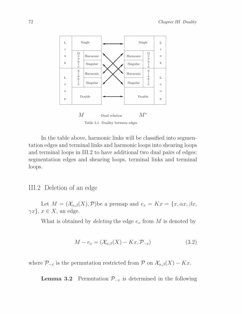
72 Chapter III Duality- -- RIRI
L
i
n
k
Single
Harmonic
Singular
Harmonic
Harmonic
Harmonic
Singular
Singular Singular
Single
Double Double
Double
Double
L
i
n
k
L
o
o
p
L
o
o
p
Single
Single
M Dual relation M∗
Table 3.1 Duality between edges
In the table above, harmonic links will be classified into segmen-
tation edges and terminal links and harmonic loops into shearing loops
and terminal loops in III.2 to have additional two dual pairs of edges:
segmentation edges and shearing loops, terminal links and terminal
loops.
III.2 Deletion of an edge
Let M = (Xα,β(X),P)be a premap and ex = Kx = x, αx, βx,γx, x ∈ X, an edge.
What is obtained by deleting the edge ex from M is denoted by
M − ex = (Xα,β(X)−Kx,P−x) (3.2)
where P−x is the permutation restricted from P on Xα,β(X)−Kx.
Lemma 3.2 Permutation P−x is determined in the following

III.2 Deletion of an edge 73
way as when ex is not a selfloop,
P−xy =
Px(and αP−1x),
if y = P−1x(and αPx);Pγx( αP−1γx),
if y = P−1γx(and αPγx);Py, otherwise,
(3.3)
and when ex is a selfloop with γx ∈ (x)P,
P−xy =
Px(and αP−1x),
if y = P−1x(and αPx);Pγx(and αP−1γx),
if y = P−1x(and αPγx);Py, otherwise,
(3.4)
otherwise, i.e., γx 6∈ (x)P , γx is replaced by βx in (3.4).
Proof When ex is not a selfloop. Because only vertices (x)P and
(γx)P are, respectively, changed in M − ex from M as
(P−1x)P−x= (P−1x,P2x, · · · ,P−2x)
and
(P−1γx)P−x= (P−1γx,Pγx, · · · ,P−2γx)
(Fig.3.2(a)⇒(b)). This implies (3.3).
When ex is a selfloop with γx ∈ (x)P . Because only vertex (x)Pis changed in M − ex from M as
(P−1x)P−x= (P−1x,Px, · · · ,P−1γx,Pγx, · · · ,P−2x)
(Fig.3.2(c)→(d)), or
(P−1x)P−x= (P−1x,Px, · · · ,P−1βx,Pβx, · · · ,P−2x)
(Fig.3.2(c)→(d) in parentheses) according as γx ∈ (x)P, or not.
The former is (3.4). The latter is what is obtained from (3.4)
with γx is replaced by βx.

74 Chapter III Duality
In Fig.3.2, the left two figures are parts of the original map and
the right two figures, the results by deleting the edge Kx.
Further, Fig.3.3–9 are all like this without specification.
I6 j3x
Pγx
P−1γx
P−1x
Px
I j3Pγx
P−1γx
P−1x
Px
(a) (b)
- j Pγx(Pβx)
γx(βx)3x
Px
P−1γx
(P−1βx)I I j Pγx(Pβx)
3Px
P−1γx
(P−1βx)
P−1xP
−1x
(c) (d)
Fig.3.2 Deletion of an edge
Lemma 3.3 For a premap M = (X ,P), M − ex = (X −

III.2 Deletion of an edge 75
Kx,P−x) is also a premap. And, the number of transitive blocks
in M − ex is not less than that in M .
Proof Because P is basic for α, from Lemma 3.2 P−x is also
basic for α. Because P satisfies the conjugate axiom for α, from
Lemma 3.2 and Theorem 2.3 P−x is also satisfies the conjugate axiom
for α. The first statement is done.
Because any nontransitive pair of elements in M is never transi-
tive in M − ex, the second statement is done.
If ex is an edge of a premap M such that M − ex has more
transitive blocks than M does, then ex is called a segmentation edge. If
an edge has its one end formed by only one semiedge of the edge itself,
then it is called an terminal link. From the symmetry of elements in a
quadricell, (x) can be assumed as the 1-vertex incident with a terminal
link without loss of generality. Since (Pγ)γx = Px = x, γx ∈ (x)Pγ.
Hence, a terminal link is always a harmonic link. However, a harmonic
link is unnecessary to be a terminal link. This point can be seen in
the following theorem.
Theorem 3.4 For a mapM = (X ,P), M−ex = (X−Kx,P−x)
is a map if, and only if, ex is not a harmonic link of M except for
terminal link.
Proof When 〈x, γx〉 ⊆ (x)Pγ, i.e., ex is a terminal link, Because
no isolated vertex in any premap, from Lemma 3.3, M − ex = (X −Kx,P−x) is a map. In what follows, this case is not considered again.
Necessity. Suppose M − ex is a map, but ex is a harmonic link of
M . Because Pγ−1x and Pγ−1γx 6= x(〈x, γx〉 6⊆ (x)Pγ) for group ΨJ ′,
J ′ = P−x, α, β, are not transitive on the set X −Kx, M − ex is not
a map. This is a contradiction to the assumption.
Sufficiency. Because M is a map, P−x is basic. From Theorem
2.3, P−x satisfies the conjugate axiom. Then, based on Table 3.1, two
cases should be discussed for the transitivity.
(i) When ex is a single edge(including single loops!) or singular
link of M . Because ex is not a cut-edge of its under graph G(M),

76 Chapter III Duality
G(M − ex) is connected. From Theorem 2.6, P−x for group ΨJ ′ is
transitive on the set X −Kx. Thus, M − ex is a map.
(ii) When ex is a double loop of M . Because
((Pγ)−1x)P−x= ((Pγ)−1x,Pαx, · · · ,
βPβx,Pγx, · · · , (Pγ)−2)αx),
we have Px = β(Pγ)x with (Pγ)−1αx and Pβx = β(βPβx) are
transitive in M − ex. Hence, M − ex is a map as well.
From the proof of the theorem, a much fundamental conclusion
is soon deduced.
Corollary 3.1 In a map M , an edge ex is a segmentation edge
if, and only if, ex is a harmonic link except for terminal links. And,
ex is a harmonic link if, and only if, it is a cut-edge of graph G(M).
Proof To prove the first statement.
Necessity. Because ex is a segmentation edge, G(M − ex) is not
connected. ex is only a link. On the basis of Table 3.1, ex is also a
double edge. And, because ex is not singular, ex is only harmonic.
Clearly, a terminal link is not a segmentation edge in its own right.
Sufficiency. Because ex is not a terminal link, Px is distinct form
x and γx is distinct from Pγx. And, because ex is a harmonic link,
Px and Pγx are not transitive in M − ex. Thus, ex is a segmentation
edge.
To prove the second statement. Because it can be shown that ex
is a terminal link of M if, and only if, ex is an articulate edge of graph
G(M), a cut-edge as well. This statement is deduced from the first
statement.
Let M = (Xα,β(X),P) be a pregraph and ex = Kx = x, αx, βx,γx, x ∈ X, be an edge. The contraction of ex from M , denoted by
M • ex = (Xα,β(X)−Kx,P•x),is defined to be the dual of M∗ − e∗x where e∗x = x, βx, αx, γx, the
corresponding edge of ex in the dual M∗ of M . In other words, P•x =
P∗−xγ.
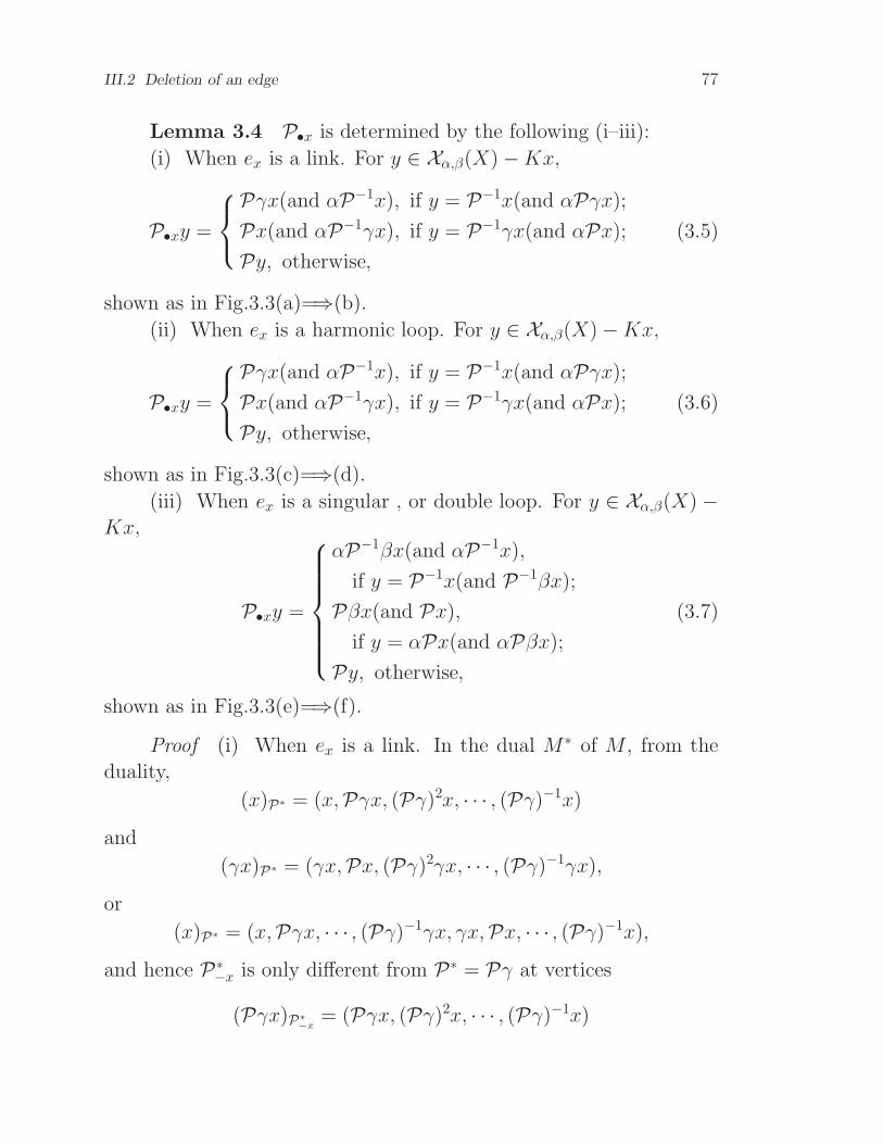
III.2 Deletion of an edge 77
Lemma 3.4 P•x is determined by the following (i–iii):
(i) When ex is a link. For y ∈ Xα,β(X)−Kx,
P•xy =
Pγx(and αP−1x), if y = P−1x(and αPγx);Px(and αP−1γx), if y = P−1γx(and αPx);Py, otherwise,
(3.5)
shown as in Fig.3.3(a)=⇒(b).
(ii) When ex is a harmonic loop. For y ∈ Xα,β(X)−Kx,
P•xy =
Pγx(and αP−1x), if y = P−1x(and αPγx);Px(and αP−1γx), if y = P−1γx(and αPx);Py, otherwise,
(3.6)
shown as in Fig.3.3(c)=⇒(d).
(iii) When ex is a singular , or double loop. For y ∈ Xα,β(X)−Kx,
P•xy =
αP−1βx(and αP−1x),
if y = P−1x(and P−1βx);
Pβx(and Px),if y = αPx(and αPβx);Py, otherwise,
(3.7)
shown as in Fig.3.3(e)=⇒(f).
Proof (i) When ex is a link. In the dual M∗ of M , from the
duality,
(x)P∗ = (x,Pγx, (Pγ)2x, · · · , (Pγ)−1x)
and
(γx)P∗ = (γx,Px, (Pγ)2γx, · · · , (Pγ)−1γx),
or
(x)P∗ = (x,Pγx, · · · , (Pγ)−1γx, γx,Px, · · · , (Pγ)−1x),
and hence P∗−x is only different from P∗ = Pγ at vertices
(Pγx)P∗−x
= (Pγx, (Pγ)2x, · · · , (Pγ)−1x)

78 Chapter III Duality
and
(Px)P∗−x
= (Px, (Pγ)2γx, · · · , (Pγ)−1γx)
or at vertex
(Px)P∗−x
= (Pγx, · · · , (Pγ)−1γx,Px, · · · , (Pγ)−1x)
with their conjugations according as ex is single, or double. By con-
sidering P•x = P∗−xγ,
P•x(y) = P•x(P−1γx) = P∗−xγ(P−1γx)
= P∗−x(Pγ−1γx) = Px
for y = P−1γx and
P•x(y) = P•x(P−1x) = P∗−xγ(P−1x)
= P∗−x(Pγ)−1x = Pγx
for y = P−1x. From the conjugate axiom, the cases for y = αP−1x
and y = α(Pγx) in the parentheses of (3.5) are also obtained. Then,
for other y,
P•x(y) = P∗−xγy = (Pγ)γy = Pyin the both cases. Therefore, (3.5) is true.
(ii) When ex is a harmonic loop. In a similar way to (3.5) for ex
single, (3.6) is also obtained.
iii) When ex is a singular, or double loop. In the dual M∗ of M ,
(x)P∗ = (x,Pγx, (Pγ)2x, · · · , (Pγ)−1x)
and
(αx)P∗ = (αx,Pγαx, (Pγ)2αx, · · · , (Pγ)−1αx),
or
(x)P∗ = (x,Pγx, · · · , (Pγ)−1αx, αx,Pγαx, · · · , (Pγ)−1x),
and hence
(x)P∗−x
= (Pγx, (Pγ)2x, · · · , (Pγ)−1x)

III.2 Deletion of an edge 79
and
(αx)P∗−x
= (Pγαx, (Pγ)2αx, · · · , (Pγ)−1αx)
or
(x)P∗−x
= (Pγx, · · · , (Pγ)−1αx,Pγαx, · · · , (Pγ)−1x)
with their conjugations according as ex is singular, or double. By
considering P•x = P∗−xγ,
P•x(y) = P•x(αPx) = P∗−xγ(αPx)= P∗−xγ(P−1αx) = P∗−x((Pγ)−1αx)
= Pγαx = Pβxfor y = αPx and
P•x(y) = P•x(P−1x) = P∗−xγ(P−1x)
= P∗−x((Pγ)−1x) = Pγx= Pαβx = αP−1βx
for y = P−1x. From the conjugate axiom, the cases for y = Pβx and
αPβx are also obtained. Then, for all other y,
P•x(y) = P∗−xγy = (Pγ)γy = Py.This is (3.7).
I6 j3
x
Pγx
P−1γx
P−1x
Px
I j3Pγx
P−1γx
P−1x
Px
(a) (b)
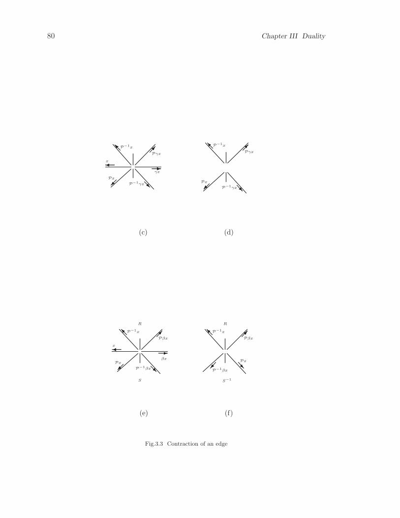
80 Chapter III Duality
I RPx
P−1γx
-γx
P−1x
Pγx RPx
P−1γx
x I P−1x
Pγx
(c) (d)
I R I R
R RP−1x
Pβx
P−1x
Pβx
S S−1
Px
P−1βx
Px
P−1βx
-x
βx
(e) (f)
Fig.3.3 Contraction of an edge

III.2 Deletion of an edge 81
From Lemma 3.4, it is seen that in the constriction of edge ex on
a premap only if ex is not a selfloop, two vertices (x)P and (γx)P are
composed of one vertex
(P−1x)P•x= (P−1x,Pγx, · · · ,P−1γx,Px, · · · ,P−2x)
(Fig.3.3(a)⇒(b)); if ex is a harmonic loop, vertex (x)P is divided into
two vertices
(P−1x)P•x= (P−1x,Pγx, · · · ,P−2x)
and
(P−1γx)P•x= (P−1γx,Px, · · · ,P−2γx)
(Fig.3.2(c)⇒(d)); and if ex is a singular, or double loop, vertex (x)Pbecomes vertex
(Px)P•x= (Px, · · · ,P−1βx, αP−1x, · · · , αPβx)
(Fig.3.3(e)⇒(f)).
Lemma 3.5 For a premap M , M •ex is always a premap. And,
the number of transitive blocks in M • ex is not less than that in M .
Proof From Lemma 3.3 and the duality, the first statement is
true. Because any nontransitive pair of elements in M is never tran-
sitive in M • ex from Lemma 3.4, the second statement is true.
If a harmonic loop ex has (x)Pγ = (x), or (γx)Pγ = (γx), then it
is called a terminal loop. If the two elements of a co-semiedge appear
in a vertex in succession, then the edge is called a twist loop.
Lemma 3.6 For an edge ex of a map M , ex is a terminal loop
if, and only if, e∗x is an terminal link in M∗. And, ex is a twist loop if,
and only if, e∗x is a twist loop.
Proof A direct result deduced from the duality.
Theorem 3.5 For an edge ex of a map M = (Xα,β(X),P),
M • ex is a map if, and only if, ex is not a harmonic loop but terminal
loop.
82 Chapter III Duality
Proof Because for a terminal loop ex, M • ex is always a map.
In what follows, this case is excluded.
Necessity. Suppose M • ex is a map but ex is a harmonic loop.
Since e∗x is a harmonic link in M∗(Table 3.1), from Theorem 3.4 and
Lemma 3.1, P−1x and Px are, respectively, belonging to two distinct
transitive blocks of M . From Lemma 3.4(ii), M •ex has two transitive
blocks. This contradicts to that M • ex is a map.
Sufficiency. Since ex is not a harmonic loop, only two cases should
be considered as ex is not a loop or ex is a singular loop. For the former,
in spite of a single or double edge, from Lemma 3.4(i), M •ex is a map.
For the latter, from Lemma 3.4(iii), M • ex = M − ex is also a map.
Therefore, the theorem is done.
If a loop ex has that P−1x and Px are in distinct noncuttable
blocks, then it is called a shearing loop . From Theorem 3.5, all shear-
ing loops are harmonic. However, the converse case is unnecessarily
true.
Corollary 3.2 In a map M , an edge ex is a shearing loop if,
and only if, e∗x is a harmonic, but not terminal loop in M∗.
Proof A direct result of Theorem 3.5.
Theorem 3.6 The dual of premapM−ex is the premapM∗•e∗x,where M∗ is the dual of M and e∗x in M∗ is the corresponding edge of
ex in M .
Proof(1) Because M∗ • e∗x is the dual of (M∗)∗− e∗∗x = M − ex,
by the symmetry of the duality the theorem holds.
However, if the contraction of ex on M is defined by (3.5–7), then
the theorem can also be proved.
Proof(2) Based on Table 3.1, four cases should be discussed.
(i) In M , ex is a single link, and hence e∗x is a single link in M∗.Since
(Pγx)P−xγ = (Pγx)P∗•x, (Px)P−x
= (Px)P∗•xγ

III.2 Deletion of an edge 83
and (Pγx)P−x= (Pγx)P∗
•xγ,
(M − ex)∗ = M∗ • e∗x.
(ii) In M , ex is a harmonic link, and hence e∗x is a harmonic loop
in M∗(Dually, in M , ex is a harmonic loop, and hence e∗x is a harmonic
link in M∗). Now, (x)Pγ = (x)P∗. According as ex is a terminal link
or not, a transitive block of M becomes one or two transitive blocks
in M − ex. Meanwhile, According as e∗x is a terminal loop or not, a
transitive block of M∗ becomes one or two transitive blocks of M∗•e∗x.By considering the changes in vertices and faces, (M − ex)
∗ = M∗ • e∗xis found.
(iii) In M , ex is a singular link, and hence e∗x is a singular loop
in M∗(Dually, In M , ex is a singular loop, and hence e∗x is a singular
link in M∗). Since
(P−1x)P−x= (P−1x)P∗
•xγ
and
(P−1γx)P−x= (P−1γx)P∗
•xγ,
in view of (Pγx)P−xγ = (Pγx)P∗•x
we have (M − ex)∗ = M∗ • e∗x.
(iv) In M , ex is a double loop, and hence e∗x is a double loop in
M∗. Since
(Px)P−x= (Px)P∗
•xγ
and
(Px)P−xγ = (Px)P∗•x,
we have (M − ex)∗ = M∗ • e∗x.
Corollary 3.3 In a map, an edge is a harmonic link if, and
only if, the corresponding edge in its dual is a harmonic loop. And,
an edge is a segmentation edge if, and only if, the corresponding edge
in its dual is a shearing loop.
Proof A direct result of Theorem 3.6.

84 Chapter III Duality
Example 3.2 Map M = (Kx+Ky +Kz,P) where
P = (x, βy, γz)(y, z, γx)
and its dual M∗ = (K∗x+K∗y +K∗z,P∗) where
P∗ = Pγ = (x, y, αx, αz, γy, z),
are, respectively, shown in Fig.3.4(a) and (b). Here, K = 1, α, β, γand K∗ = 1, β, α, γ are used to distinguish α and β.
Map M − ex = (Ky +Kz,P−x) where P−x = (βy, γz)(y, z) and
its dual (M − ex)∗ = (K∗y + K∗z, (P−x)
∗), where (P−x)∗ = P−xγ =
(y, βz, αy, γz), are, respectively, shown in Fig.3.4(c) and (d). It is
easily seen that (M − ex)∗ = M∗ • e∗x.
-- YY 6 3j?+x x
αx
βy
γzy
z
βx
y
αx
αz
γy
z
(a) M (b) M∗

III.3 Addition of an edge 85
- 6 -?z
γz
βy
y
y
βz
γz
αy
(c) M − ex (d) (M − ex)∗
Fig.3.4 Duality between deletion and contraction
III.3 Addition of an edge
Let M = (Xα,β,P) be a premap, ex = Kx = x, αx, βx, γx, and
x 6∈ Xα,β. Write as
M + ex = (Xα,β +Kx,P+x),
where P+x is determined from P in the following manner. For any
y ∈ Xα,β and two given angles 〈l,Pαl〉 and 〈t,Pαt〉, if l and t are
not at the same vertex, or at the same vertex and ex as a harmonic
loop(assume t ∈ (l)P without loss of generality), then
P+xy =
t(and αx), if y = x(and αt);
Pαt(and x), if y = αx(and αPαt);l(and βx), if y = γx(and αl);
Pαl(and γx), if y = βx(and αPαl);Py, otherwise,
(3.8)

86 Chapter III Duality
Æ MN - 6?I
Rx
x
γx
βx
t
Pαl
Pαt
l
t Pαt
Pαl l
(a) For (3.8) (b) For (3.9)
Fig.3.5 Appending an edge
shown in Fig.3.5(a), otherwise, i.e., ex is a double, or singular loop
(assume t ∈ (l)P without loss of generality),
P+xy =
t(and αx), if y = x(and αt);
Pαt(and x), if y = αx(andαPαt);l(andβx), if y = γx(and αl);
Pαl(and βx), if y = γx(and αPαl);Py, otherwise,
(3.9)
as shown in Fig.3.5(b).
Such a transformation from M into M + ex is called appending
an edge ex.
Lemma 3.7 For a premap M = (X ,P), M + ex = (X +
Kx,P+x) is also a premap. And, the number of transitive blocks
in M + ex is not greater than that in M .
Proof From (3.8) and (3.9), P+x is basic. In virtue of Theorem
2.3, it suffices to show that the orbits of P+x are partitioned into
conjugate pairs for the conjugate axiom. In fact, if l and t are at
distinct vertices, then P+x is obtained from P in replacing two vertices

III.3 Addition of an edge 87
(t)P and (l)P by respective
(t)P+x= (t,Pt, · · · , αPαt, x)
and
(l)P+x= (l,Pl, · · · , αPαl, γx),
or βx is substituted for γx. If l and t are at the same vertex, then
P+x is obtained from P in replacing the vertex (l)P by
(l)P+x= (l,Pl, · · · , αPαt, x, t,Pt, · · · , αPαl, γx)
or
(l)P+x= (l,Pl, · · · , αPαt, x, t,Pt, · · · , αPαl, βx)
according as ex is a harmonic loop or not. This shows that the orbits
of P+x are partitioned into conjugate pairs for α.
Note 3.2 On the degenerate case t = l, if ex is a harmonic
loop, then
(l)P+x= (l,Pl, · · · , αPαl, γx, x);
otherwise, i.e., ex is a twist loop,
(l)P+x= (l,Pl, · · · , αPαl, βx, x).
Theorem 3.7 For a premap, not a map, M = (Xα,β,P), the
number of transitive blocks of M + ex is less than that of M if, and
only if, ex ia a segmentation edge. If M is a map, then M + ex is also
a map.
Proof Since the number of components of graph G(M + ex) is
less than that of G(M) if, and only if, ex is a cut-edge which is not
articulate, the first statement is deduced from Corollary 3.1.
Because the transitivity between two elements in the ground set
of M under appending an edge is unchanged, the second statement is
valid.
Note 3.3 Let M ′ = (X + Kx,P ′) = M + ex for M = (X ,P).
Because P ′−x = P , M is obtained by the deletion of the edge ex from
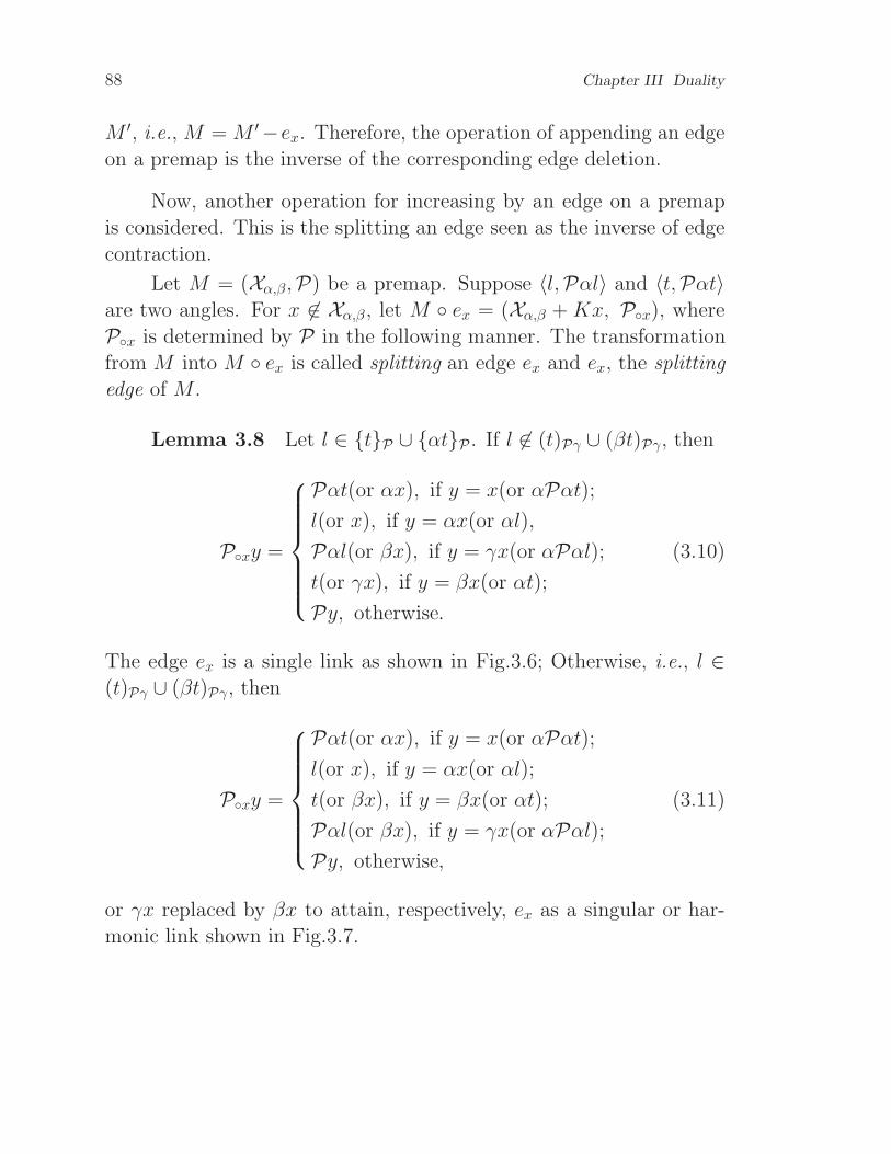
88 Chapter III Duality
M ′, i.e., M = M ′−ex. Therefore, the operation of appending an edge
on a premap is the inverse of the corresponding edge deletion.
Now, another operation for increasing by an edge on a premap
is considered. This is the splitting an edge seen as the inverse of edge
contraction.
Let M = (Xα,β,P) be a premap. Suppose 〈l,Pαl〉 and 〈t,Pαt〉are two angles. For x 6∈ Xα,β , let M ex = (Xα,β + Kx, Px), where
Px is determined by P in the following manner. The transformation
from M into M ex is called splitting an edge ex and ex, the splitting
edge of M .
Lemma 3.8 Let l ∈ tP ∪ αtP . If l 6∈ (t)Pγ ∪ (βt)Pγ, then
Pxy =
Pαt(or αx), if y = x(or αPαt);l(or x), if y = αx(or αl),
Pαl(or βx), if y = γx(or αPαl);t(or γx), if y = βx(or αt);
Py, otherwise.
(3.10)
The edge ex is a single link as shown in Fig.3.6; Otherwise, i.e., l ∈(t)Pγ ∪ (βt)Pγ, then
Pxy =
Pαt(or αx), if y = x(or αPαt);l(or x), if y = αx(or αl);
t(or βx), if y = βx(or αt);
Pαl(or βx), if y = γx(or αPαl);Py, otherwise,
(3.11)
or γx replaced by βx to attain, respectively, ex as a singular or har-
monic link shown in Fig.3.7.
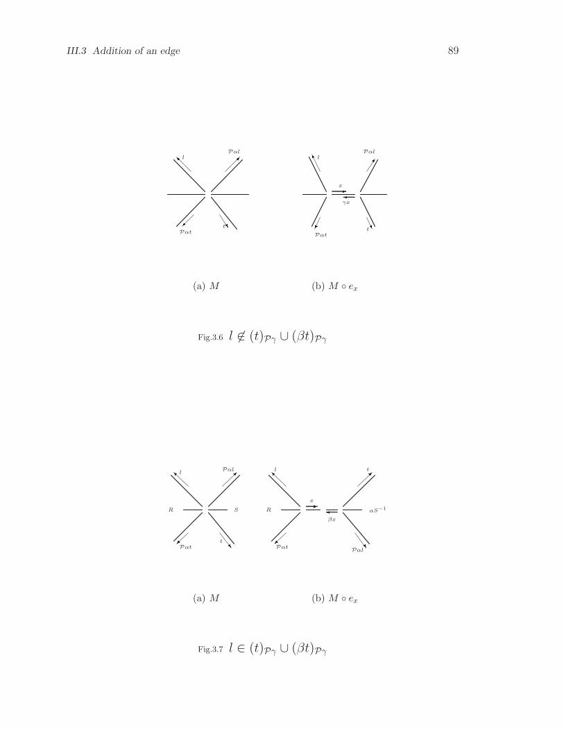
III.3 Addition of an edge 89
I ^
K U-l l
PαtPαt
Pαl Pαl
tt
x
γx
(a) M (b) M ex
Fig.3.6 l 6∈ (t)Pγ ∪ (βt)Pγ
I w
I wR
l
R-
S αS−1
l
x
βx
t
Pαl
Pαl
tPαt Pαt
(a) M (b) M ex
Fig.3.7 l ∈ (t)Pγ ∪ (βt)Pγ

90 Chapter III Duality
Proof Since l ∈ tP ∪ αtP , l and t are at the same vertex.
Thus, ex is a link. If l 6∈ (t)Pγ ∪ (βt)Pγ, i.e., l is in a face different
from that t is in, or in other words, ex is single, then by the reason as
(Px)•x is different from only the vertex
(Pxx)(Px)•x= (Pαt, · · · , αl,Pαl, · · · , αt)
where Pxx = Pαt shown in Fig.3.6, from Lemma 3.4(i), (Px)•x = P .
Otherwise, according as ex is singular or harmonic, (Px)•x is different
from only the vertex
(Pxx)(Px)•x= (Pαt, · · · , αl,Pαl, · · · , αt)
or
(Pαt, · · · , αl, t, · · · , αPαl)shown in Fig.3.7. From Lemma 3.4(i) again, (Px)•x = P .
Lemma 3.9 Let l 6∈ tP ∪ αtP . If t and l are not transitive
on M , then
Pxy =
Pαl(or αx), if y = x(or αPαl);t(or x), if y = αx(or αt);
Pαt(or βx), if y = γx(or αPαt);l(or γx), if y = βx(or αl);
Py, otherwise
(3.12)
as shown in Fig.3.8 where ex is a harmonic loop.
Otherwise, i.e., t and l are transitive on M , then
Pxy =
Pαl(or αx), if y = x(or αPαl);Pαt(or x), if y = αx(or αPαt);l(or βx), if y = γx(or αl);
t(or γx), if y = βx(or αt);
Py, otherwise,
(3.13)
as shown in Fig.3.9 where ex is a singular, or harmonic loop according
as it is incident with two faces, or one face.

III.3 Addition of an edge 91
Y j1 - >~l
Pαt
l
Pαt
PαlPαl
tt
x
γx
(a) M (b) M ex
Fig.3.8 t and l nontransitive
R
S
R
αS−1
Y j1 - >~l
Pαt
l
t
PαlPαl
tPαt
x
βx
(a) M (b) M ex
Fig.3.9 t and l transitive
Proof Since l ∈ tP ∪ αtP , l and t are at the same vertex.
Thus, ex is a link. If l 6∈ (t)Pγ ∪ (βt)Pγ, i.e., l is in a face different
from that t is in, or in other words, ex is single, then by the reason as

92 Chapter III Duality
(Px)•x is different from only the vertex
(Pxx)(Px)•x= (Pαt, · · · , αl,Pαl, · · · , αt)
where Pxx = Pαt shown in Fig.3.6, from Lemma 3.4(i), (Px)•x = P .
Otherwise, according as ex is singular or harmonic, (Px)•x is different
from only the vertex
(Pxx)(Px)•x= (Pαt, · · · , αl,Pαl, · · · , αt)
or
(Pαt, · · · , αl, t, · · · , αPαl)shown in Fig.3.7. From Lemma 3.4(i) again, (Px)•x = P .
Lemma 3.10 If M = (X ,P) is a premap, then for any x ∈ X ,
M ex = (X +Kx,Px) is also a premap. And, M ex has the number
of its transitive blocks not greater than M does.
Proof From Lemmas 3.8–9, permutation Px is basic and parti-
tioned into conjugate pairs for α. Then by Theorem 2.3, M x is also
a premap. This is the first statement. Because splitting an edge does
not changing the transitivity of any pair of elements in X , the second
statement holds.
Lemma 3.11 Edge ex is a harmonic loop on M ex if, and only
if, Pxx and Pxγx are not transitive on M .
Proof Necessity. Because the splitting edge ex is a harmonic
loop on M , it is in the case (3.12). As shown in Fig. 3.8, Pxβx(= l)
and Pxαx(= t) are not transitive on M . Hence, by the symmetry
among elements inKx, Pxx and Pxγx are not transitive onM either.
Sufficiency. Because Pxβx(= l) and Pxαx(= t) are not tran-
sitive on M , only l 6∈ tP ∪ αtP is possible. This is the case for
(3.12). Thus, ex is a harmonic loop.
Theorem 3.8 For a premap M = (Xα,β,P) not a map, the
number of transitive blocks in M ex is less than that in M if, and
only if, ex is a harmonic loop. If M is a map, then M ex is also a
map.

III.3 Addition of an edge 93
Proof From Lemma 3.11, the number of transitive blocks in
M ex is less than that in M if, and only if, ex is a segmentation
edge in M + ex. This is the first statement. Because splitting an edge
in a map does not changing the transitivity, the second statement is
obtained.
Lemma 3.12 Edge ex = x, αx, βx, γx is appended in premap
M if, and only if, edge e∗x = x, βx, αx, γx is split to in premap M∗.
Proof Necessity. (1) If ex is a single edge of M + ex, i.e., γx 6∈(x)P+xγ ∪ (βx)P+xγ, then (x)P∗
+xand (γx)P∗
+xare two vertices on (M +
ex)∗. Hence, from (3.10–11), e∗x is the splitting edge from the vertex
(P∗+xx)P∗ = (P∗+xx, · · · , (P∗+x)−1x,P∗+xγx, · · · , (P∗+x)
−1γx)
on M∗.(2) Otherwise, i.e., ex is a double edge on M + ex. Thus, γx ∈
(x)P+xγ ∪ (βx)P+xγ. Two cases should be considered.
(i) If γx ∈ (x)P+xγ, then ex is a segmentation edge on M +
ex. From Corollary 3.1, P∗+xx and P∗+xγx are not transitive on M .
Furthermore, from (3.12), e∗x is a splitting edge(a harmonic loop) on
M∗.
(ii) If γx ∈ (βx)P+xγ, then from (3.13), e∗x is a splitting edge on
M∗.
Sufficiency. (1) If e∗x is not a loop onM∗e∗x, then from (3.10–11),
M has a face
(P∗xx)Pγ = (P∗xx, · · · , (P∗x)−1x,P∗xγx, · · · , (P∗x)−1γx).
From (3.6), ex is an appending edge between
angle 〈αP∗x−1x,P∗xγx〉 and angle 〈αP∗x−1γx,P∗xx〉in a face of M , as shown in (3.8–9).
(2) Otherwise, i.e., e∗x is a loop. From (3.12–13), there are two
faces on M with an angle each. Such two angles determine the ap-
pending edge ex on M .
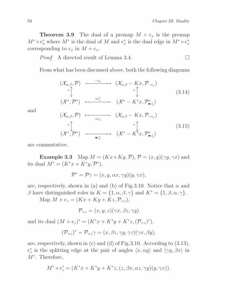
94 Chapter III Duality
Theorem 3.9 The dual of a premap M + ex is the premap
M∗ e∗x where M∗ is the dual of M and e∗x is the dual edge in M∗ e∗xcorresponding to ex in M + ex.
Proof A directed result of Lemma 3.4.
From what has been discussed above, both the following diagrams
(Xα,β,P)−ex−−−−−−−−→ (Xα,β −Kx,P−ex
)∗xy ∗
xy
(X ∗,P∗) e∗x←−−−−−−−− (X ∗ −K∗x,P∗•e∗x)(3.14)
and(Xα,β,P) ←−−−−−−−−
+ex
(Xα,β −Kx,P−ex)
∗xy ∗
xy(X ∗,P∗) −−−−−−−−→
•e∗x(X ∗ −K∗x,P∗•e∗x)
(3.15)
are commutative.
Example 3.3 Map M = (Kx+Ky,P), P = (x, y)(γy, γx) and
its dual M∗ = (K∗x+K∗y,P∗),
P∗ = Pγ = (x, y, αx, γy)(y, γx),
are, respectively, shown in (a) and (b) of Fig.3.10. Notice that α and
β have distinguished roles in K = 1, α, β, γ and K∗ = 1, β, α, γ.Map M + ez = (Kx+Ky +Kz,P+z),
P+z = (x, y, z)(γx, βz, γy)
and its dual (M + ez)∗ = (K∗x+K∗y +K∗z, (P+z)
∗),
(P+z)∗ = P+zγ = (x, βz, γy, γz)(γx, βy),
are, respectively, shown in (c) and (d) of Fig.3.10. According to (3.13),
e∗z is the splitting edge at the pair of angles 〈x, αy〉 and 〈γy, βx〉 in
M∗. Therefore,
M∗ e∗z = (K∗x+K∗y +K∗z, (z, βx, αz, γy)(y, γx)).

III.3 Addition of an edge 95
If βy is seen as y, then M∗ e∗z = (M + ez)∗.
II+s33 II+
s33γx
γy
αx
αyxy βx
γx
y
αyxγy
(a) M (b) M∗
II=s3
66 6γx
γy
αx
αyxy ??
βz
z
βx
γy
6?
γx?αy
y
x
z
βz
--γz
αz
(c) M + ez (d) (M + ez)∗
Fig.3.10 Duality between appending and splitting an edge
Based on Theorem 3.9, in a premap M = (X ,P), splitting an
edge ex attains M ex which is just M∗ + e∗x obtained by appending
the edge e∗x in its dual M∗ = (X ∗,P∗).

96 Chapter III Duality
III.4 Basic transformation
In a premap M = (Xα,β,P), the deletion of a single edge ex
is called basic deleting an edge and its result is denoted by M −b
ex. The contraction of a link ex is called basic contracting an edge,
and its result is denoted by M •b ex. The two operations are, in all,
called basic subtracting an edge. Similarly, appending a single edge
is called basic appending an edge, and splitting a link is called basic
splitting an edge. Such two operations are, in all, called basic adding
an edge. Apparently, M +b ex and M b ex are the results of basic
adding an edge ex on M in their own right. Basic subtracting and
basic adding an edge are in all called basic transformation. From what
we have known above, A premap becomes another premap under basic
transformation.
Theorem 3.10 Suppose M ′ is a premap obtained by basic
transformation from premap M , then M ′ is a map if, and only if,
M is a map.
Proof Because a single edge is never a harmonic link, from The-
orem 3.4 the theorem holds for basic deleting an edge. Because a link
is never a harmonic loop, from Theorem 3.5, the theorem holds for
basic contracting an edge. Then, from Theorem 3.7–8, the theorem
holds for basic adding an edge.
Furthermore, for basic transformation, the following conclusion
can also be done.
Theorem 3.11 Let M = (X ,P) be a map and M∗ = (X ∗,P∗),its dual. Then, for any single edge ex in M , (M −b ex)
∗ = M∗ •b e∗xand for a single edge ex not in M , (M +b ex)
∗ = M∗ b e∗x. Conversely,
for any link ex in M , M •b ex = M∗ −b e∗x and for a link ex not in M ,
M b ex = M∗ +b e∗x.
Proof Based on the duality between edges as shown in Table
3.1, the statements are meaningful. From Theorem 3.6 and Theorem
3.9, the fist statement is true. In virtue of the duality, the second

III.4 Basic transformation 97
statement is true.
From this theorem, the following two diagrams are seen to be
commutative:
(Xα,β,P)−bex−−−−−−−−→ (Xα,β −Kx,P−bex
)∗xy ∗
xy
(X ∗,P∗) be∗x←−−−−−−−− (X ∗ −K∗x,P∗•be∗x)(3.16)
and(Xα,β,P) ←−−−−−−−−
+bex
(Xα,β −Kx,P−bex)
∗xy ∗
xy(X ∗,P∗) −−−−−−−−→
•be∗x(X ∗ −K∗x,P∗•be∗x)
(3.17)
On the basis of basic transformation, an equivalence can be es-
tablished for classifying maps in agreement with the classification of
surfaces.

Activities on Chapter III
III.5 Observations
O3.1 Observe the condition for two permutations Per1 and Per2
satisfying (3.1) on the same ground set.
O3.2 Given a tree(e.g., the star of 5 edges), observe how many
maps are there for their dual maps all having the tree as under graph.
O3.3 Write the dual of map M = (Kx, (x, βx)). If a map has
its dual with the same under graph, then it is said to be self-dual for
the graph. Observe if M is self-dual for its under graph.
O3.4 Provide a map which is cuttable and its under graph with
a cut-vertex.
O3.5 How to distinguish the cuttability of a map and the sep-
arability of its under graph?
O3.6 Is the under graph of the dual of a Eulerian map bipar-
tite? If yes, explain the why; otherwise, by an example.
O3.7 Is the dual of a preproper map(no double edge) always a
preproper map? If yes, explain the why; otherwise, by an example.
O3.8 Is the dual of a proper map(each face formed by a circuit
in its under graph) always a proper map? If yes, explain the why;
otherwise, by an example.
O3.9 Is the dual of a polygonal map(two face with at most one
edge in common) always a polygonal map? If yes, explain the why;

III.6 Exercises 99
otherwise, by an example.
O3.10 Is the under graph of the dual of a map with 3-connected
under graph still 3-connected? If yes, explain the why; otherwise, by
an example.
III.6 Exercises
E3.1 Prove that the under graph of a map M = (X ,P) is a
tree if, and only if, its dual M∗ has the following three properties:
(i) M∗ has only one vertex;
(ii) For any x ∈ X , x and γx are in the same orbit of P∗;(iii) For any y ∈ (x)P∗, there is no subsequence x, y, γx, γy or
x, γy, γx, y in its cycle.
For a mapM = (X (X),P) and S ⊆ X, letM [KS] = (KS,P [KS])
where P [KS] is the restriction of P on KS = KS, and M [KS] is said
to be induced on KS from M . Generally speaking, M [KS] is not a
map, but always a premap. A cocircuit of a graph with all of its edges
incident to the same vertex is called a proper cocircuit .
E3.2 Let M − ES = M [X − KS], ES = ex|∀x ∈ S. Prove
that M − ES, S ⊆ X, is a map if, and only if, there is no proper
cocircuit of G[M ] on graph G(M [KS]).
A proper circuit of a map M is such a set C of edges that C∗ =
e∗|∀e ∈ C is a proper cocircuit of G[M∗].
E3.3 Let H = G[M ] and MH be the set of all maps whose
under graphs are H. Prove that if C is a proper circuit of a map M ,
then it is a proper circuit of all N ∈MH .
E3.4 Let M • ES = (M∗ − E∗S)∗ where M∗ is the dual of M
and E∗S = e∗x|∀x ∈ S. Prove that M • ES is a map if, and only if,
ES is a proper circuit of M .
E3.5 Prove that a map M is on the sphere if, and only if, each
face of its dual M∗ corresponds to a proper cocircuit of M .

100 Activities on Chapter III
If a map has its dual Eulerian, then it is called a dual Eulerian
map.
E3.6 Prove that a map is a dual Eulerian map if, and only if,
each of its faces is incident with even number of edges.
If a preproper dual Eulerian map has each of its faces partition-
able into circuits, then it is called a even assigned map . A map is
called bipartite when its under graph is bipartite.
E3.7 Prove that a dual Eulerian map is bipartite if, and only
if, it is even assigned.
E3.8 Prove that a quadrangulation is bipartite if, and only if,
it is without loop.
For a loopless quadrangulation Q = (Xα,β,Q), from E3.8, its
vertex set V can be partitioned into two subsets V1 and V2 such that
the two ends of each edge are never in the same subset. Such a subset
of vertices is called an independent set. X (1)α1,β1
and X (2)α2,β2
stand for
the sets of elements in Xα,β incident to, respectively, V1 and V2[Deh1,
Gau1, MuS1].
E3.9 Let σ = βQγ, γ = αβ. Prove that (σx, σQαx), x ∈ Xα,β,
is an angle.
Angles (σx, σQαx) and (x,Qαx) as shown in E3.9 are called an
independent pair . Thus, each face in a quadrangulation has exactly
two independent pairs of angles.
E3.10 Let K1 = 1, α1, β1, γ1, γ1 = α1β1. And, α1 = Q and
β1 = βQγ(= σ as shown in E3.9). Prove
(i) K1 is the Klein group of four elements;
(ii) X (1)α1,β1
=∑
vx∈V1
∑
y∈xQK1y;
(iii) Q1 = (X (1)α1,β1
,Q−11 ) is a map, where Q1 is the restriction of
Q on X (1)α1,β1
.
Similarly to E3.10, from V2, another map Q2 can be deduced. Q1
and Q2 are called the incident pair of the quadrangulation.
III.7 Researches 101
E3.11 Prove that the two maps in the incident pair of a quad-
rangulation are mutually dual.
E3.12 Prove that any planar quadrangulation is loopless.
E3.13 Let A and B be the sets of, respective all planar quad-
rangulations and all dual pairs of planar maps. Establish a 1–to–1
correspondence between A and B(i.e., bijection).
III.7 Researches
For a map, if the basic deletion of an edge can not be done
anymore, then the map is said to be basic deleting edge irreducible.
Similarly, if the basic contraction of an edge can not be done on a
map anymore, then the map is said to be basic contracting irreducible.
R3.1 Given the size, determine the number of self-dual maps
as an integral function of the size, or provide a way to list all the self-
dual maps of the same size and deduce a relation among the numbers
of different sizes.
R3.2 Given the size, determine the number of maps all basic
deleting irreducible as an integral function of the size, or provide a
way to list all such maps with the same size and deduce a relation
among the numbers of different sizes.
R3.3 Given the size, determine the number of maps all basic
contracting irreducible as an integral function of the size, or provide
a way to list all such maps with the same size and deduce a relation
among the numbers of different sizes.
R3.4 For any given graph, determine the number of maps all
basic deleting irreducible with the same under graph, or provide a way
to list all such maps with the same size and deduce a relation among
the numbers of different sizes.
R3.5 For any given map, determine the number of all basic
deleting irreducible maps obtained from the map by basic deletion, or

102 Activities on Chapter III
provide a way to list all such maps with the same size and deduce a
relation among the numbers of different sizes.
R3.6 For a given graph, determine the number of maps all basic
contracting irreducible with the same under graph, or provide a way to
list such maps and deduce a relation among the numbers of different
sizes.
R3.7 For a given map, determine the number of all basic con-
tracting irreducible maps obtained from the map by basic contraction,
or provide a way to list such maps and deduce a relation among the
numbers of different sizes.
If a map is basic both deleting and contracting irreducible, then
it is said to be basic subtracting irreducible.
R3.8 Given the size, determine the number of basic subtracting
irreducible maps as an integral function of the size, or provide a way
to list all such maps with the same size and deduce a relation among
the numbers of different sizes.
R3.9 For a given graph, determine the number of maps all basic
subtracting irreducible with the same under graph, or provide a way
to list such maps and deduce a relation among the numbers of different
sizes.
R3.10 Find a relation between triangulations and quadrangu-
lations.
If a map has each of its faces pentagon, then it is called a quin-
quangulation. Similarly, the meaning of a hexagonalization.
R3.11 Justify whether or not a triangulation has a spanning
quinquangulation or hexagonalization. If do, determine its number.
R3.12 Even assigned conjecture: A bipartite graph without
cut-edge has a super map even assigned.

Chapter IV
Orientability
• The orientability is determined by the orientation for each edge
with two sides; otherwise, nonorientability.
• The basic equivalence is defined via basic transformations to show
that the orientability is an invariant in an equivalent class. This
equivalence is, in fact, the elementary equivalence on surfaces.
• The Euler characteristic is also shown to be an invariant in an
equivalent class.
• Two examples show that none of the orientability(nonorientability
as well) and the Euler characteristic can determine the equivalent
class.
IV.1 Orientation
Let M = (Xα,β,P) be a map(from Theorem 2.6, without loss of
generality for a premap), and ΨI , I = γ,P, γ = αβ = βα, be the
group generated by the set of permutations I. Now, it is known that
the number of orbits of P on Xα,β is double the number of vertices on
M and the number of orbits of Pγ on Xα,β is double the number of
faces on M . Because P ,Pγ ∈ ΨI , the number of orbits of the group
ΨI on Xα,β is not greater than any of their both.

104 Chapter IV Orientability
Lemma 4.1 The number of orbits of the group ΨI on Xα,β is
not greater than 2.
Proof Because Pγ ∈ ΨI , for any x ∈ Xα,β, xPγ ⊆ xΨI.
Here, xPγ and xΨIare the orbits of, respectively, the permutation
Pγ and the group ΨI on Xα,β. For any chosen element x ∈ Xα,β, from
P ∈ Ψ, for any y ∈ xPγ, yPγ ⊆ xΨI, and from γ ∈ Ψ,
γyPγ ⊆ γyΨI⊆ xΨI
.
In view of Theorem 2.6, at least half of elements at each vertex belong
to xΨI. Therefore, xΨI
contains at least half of elements in Xα,β .
Similarly, αxΨIcontains at least half of elements in Xα,β.
In consequence, based on the basicness of P for α, ΨI has at
most 2 orbits on Xα,β.
According to this lemma, a map M = (Xα,β,P) has only two
possibilities: group ΨI is with two, or one, orbits on Xα,β. The former
is called orientable, and the later, nonorientable .
From the proof of the lemma, an efficient algorithm can be es-
tablished for determining all the orbits of group ΨI on the ground
set.
Actually, in an orientable map, because ΨI has two orbits for α,
the ground set is partitioned into two parts of equal size. It is seen
from Lemma 4.1 that each quadricell (i.e., edge) is distinguished by
two elements in each of the two orbits. And, the two elements of an
edge in the same orbit have to be with different ends of the edge.
Thus, each of the two orbits determines the under graph of the map.
Example 4.1 Consider map M = (X ,P) where
X = Kx+Ky +Kz +Ku+Kv +Kw
and
P = (x, y, z)(γz, u, v)(γv, γy, w)(γw, γu, γx)
as shown in Fig.4.1(a). Its two faces are
(x, γw, γv, γz)

IV.1 Orientation 105
and
(γx, y, w, γu, v, γy, z, u).
In fact, for this map, group ΨI has two orbits. One is
x, γw, γv, γz, γx, y, w, γu, v, γy, z, u.
The other is what is obtained from it by multiplying α to each of all
its elements. Thus, M is orientable. Fig.4.1(b) shows that M is an
embedding of the complete graph of order 4 on the torus (yuy−1u−1).
-? 6 - -?6 - ? - 6?-6 -?γx
γx
xx
yz u
v
w
γy
y
zu
v
γy
w
γuγu
(a) (b)
Fig.4.1 An embedding of K4
Corollary 4.1 If ΨI , I = P , αβ, has two orbits on Xα,β, then
they are conjugate for both α and β.
Proof It is known from Lemma 4.1 that the two obits have the
same number of elements, i.e., half of Xα,β. Because y ∈ xΨIif, and
only if, αy ∈ αxΨIand for any Kx, αx and βx are always in the
same orbit of ΨI , this implies that αxΨI= βxΨI
different from
xΨIand hence the conclusion.
Example 4.2 Consider map N = (X ,Q) where
X = Kx+Ky +Kz +Ku+Kv +Kw
and
Q = (x, y, z)(γz, u, v)(γv, βy, w)(γw, γu, γx)
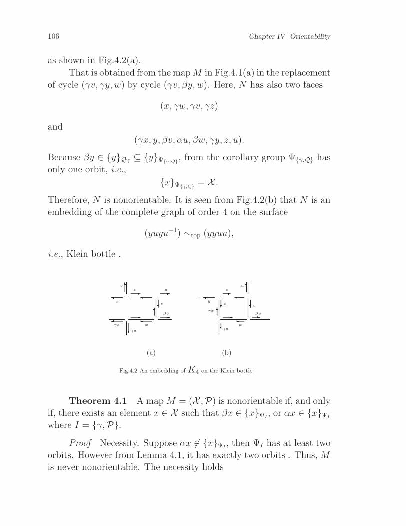
106 Chapter IV Orientability
as shown in Fig.4.2(a).
That is obtained from the mapM in Fig.4.1(a) in the replacement
of cycle (γv, γy, w) by cycle (γv, βy, w). Here, N has also two faces
(x, γw, γv, γz)
and
(γx, y, βv, αu, βw, γy, z, u).
Because βy ∈ yQγ ⊆ yΨγ,Q, from the corollary group Ψγ,Q has
only one orbit, i.e.,
xΨγ,Q= X .
Therefore, N is nonorientable. It is seen from Fig.4.2(b) that N is an
embedding of the complete graph of order 4 on the surface
(yuyu−1) ∼top (yyuu),
i.e., Klein bottle .
-? 6 - -?6 - ? - 6?-6 -?γx
γx
xx
yz u
v
w
βy
y
zu
v
βy
w
γuγu
(a) (b)
Fig.4.2 An embedding of K4 on the Klein bottle
Theorem 4.1 A map M = (X ,P) is nonorientable if, and only
if, there exists an element x ∈ X such that βx ∈ xΨI, or αx ∈ xΨI
where I = γ,P.Proof Necessity. Suppose αx 6∈ xΨI
, then ΨI has at least two
orbits. However from Lemma 4.1, it has exactly two orbits . Thus, M
is never nonorientable. The necessity holds

IV.2 Basic equivalence 107
Sufficiency. Because βx ∈ xΨI, from Corollary 4.1 it is only
possible to have x = X , i.e., ΨI has only one orbit. Hence, M is
nonorientable. This is the sufficiency.
This theorem enables us to justify the nonorientability and hence
the orientability of a map much simple. If there exists a face (x)Pγ,
denoted by Sx, such that αx ∈ Sx, or there exists a vertex (x)P ,denoted by Sx, such that βx ∈ Sx on M , then M is nonorientable(as
shown in Example 2). Otherwise, From y ∈ Sx via acting P , or γ, for
getting z 6∈ Sx, Sx is extended into
Sx ∪ zPγ ∪ zP
which is seen as a new S to see if y, αy ∈ S, or y, βy ∈ S. If it does,
thenM is nonorientable; otherwise, do the extension until |S| = |X |/2,
or S = X .
Theorem 4.2 A map M = (X ,P) is orientable if, and only if,
its dual M∗ = (X ∗,P∗) is orientable.
Proof Because P∗ = Pγ ∈ Ψγ,P(γ = αβ = βα), Ψγ,P =
Ψγ,P∗. So, for any x ∈ X = X ∗, xΨγ,P= xΨγ,P∗
. This is the
conclusion of the theorem.
IV.2 Basic equivalence
First, observe the effect for the orientability of a map via basic
transformation.
For a map M = (X ,P) and its edge ex, let M −b ex and M •b ex
be, respectively, obtained by basic deleting and basic contracting the
edge ex on M . From Theorem 3.10, M −b ex and M •b ex are both a
map .
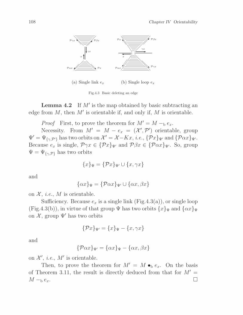
108 Chapter IV OrientabilityI 6 R? -oRx x
γxγx
Pγx
Pγx
PβxPβx
Px
Px
Pαx Pαx
(a) Single link ex (b) Single loop ex
Fig.4.3 Basic deleting an edge
Lemma 4.2 If M ′ is the map obtained by basic subtracting an
edge from M , then M ′ is orientable if, and only if, M is orientable.
Proof First, to prove the theorem for M ′ = M −b ex.
Necessity. From M ′ = M − ex = (X ′,P ′) orientable, group
Ψ′ = Ψγ,P ′ has two orbits onX ′ = X−Kx, i.e., PxΨ′ and PαxΨ′.
Because ex is single, Pγx ∈ PxΨ′ and Pβx ∈ PαxΨ′. So, group
Ψ = Ψγ,P has two orbits
xΨ = PxΨ′ ∪ x, γx
and
αxΨ = PαxΨ′ ∪ αx, βxon X , i.e., M is orientable.
Sufficiency. Because ex is a single link (Fig.4.3(a)), or single loop
(Fig.4.3(b)), in virtue of that group Ψ has two orbits xΨ and αxΨon X , group Ψ′ has two orbits
PxΨ′ = xΨ − x, γx
and
PαxΨ′ = αxΨ − αx, βxon X ′, i.e., M ′ is orientable.
Then, to prove the theorem for M ′ = M •b ex. On the basis
of Theorem 3.11, the result is directly deduced from that for M ′ =
M −b ex.

IV.2 Basic equivalence 109
Whenever that two new angles occur in the deletion of an edge
with 4 angles lost is noticed, the edge appending as the inverse of
deletion is done between the two angles. And then the same case
comes for basic deleting and basic appending an edge. In this sense,
Lemma 4.3 in what follows is seen as a direct result of Lemma 4.2.
However, it is still proved in an independent way.
For basic appending an edge, since the edge is only permitted
to be a single link or a single loop, this operation is, in fact, done by
putting the edge in the same face.
Let map M = (X ,P) have a face
(y)Pγ = (y0, y1, · · · , ys)
where y0 = y, y1 = (Pγ)y, · · ·, ys = (Pγ)−1y. Denote
M +i ex = M +b ex
when appending the edge ex in between angles 〈y,Pαy〉 and 〈yi,Pαyi〉,0 ≤ i ≤ s. From (3.10), M +i ex = M +b ex, 0 ≤ i ≤ s, are all
maps(Fig.4.4).
y - y1
yl+1
oRx
yl
yl−1
ys
y - y1
yl+1
o Rx
γx
yl
yl−1
ys
Yγx
i(a) M +0 ex (b) M +1 ex

110 Chapter IV Orientability
y - y1
yl+1
oR yl
yl−1
ys
y - y1
yl+1
- oRx
γx
yl
yl−1
ys
jx
γx
(c) M +l ex (d) M +l+1 ex
Fig.4.4 Basic appending an edge
Lemma 4.3 Maps M+iex = M+bex, 0 ≤ i ≤ s, are orientable
if, and only if, M is orientable.
Proof necessity. Since M ′ = M +i ex = (X ′,P ′), 0 ≤ i ≤ s,
are all orientable, group Ψ′ = Ψγ,P ′ has two orbits xΨ′ and αxΨ′
on X ′ = X +Kx. Because ex is a single link (Fig.4.4(a) and (c)), or
single loop (Fig.4.4(b) and (d)),
P ′x ∈ xΨ′ and P ′αx ∈ αxΨ′.
Hence, group Ψ = Ψγ,P has two orbits
P ′xΨ = xΨ′ − x, γx
and
P ′αxΨ = αxΨ′ − αx, βxon X . This implies that M is orientable.
Sufficiency. Since ex is a single link (Fig.4.4(a) and (c)), or single
loop (Fig.4.4(b) and (d)), the two orbits
xΨ′ = yΨ + x, γx
and
αxΨ′ = αyΨ + αx, βxof group Ψ′ on X ′ are deduced from the two orbits yΨ and αyΨof group Ψ on X . Therefore, M ′ is orientable.
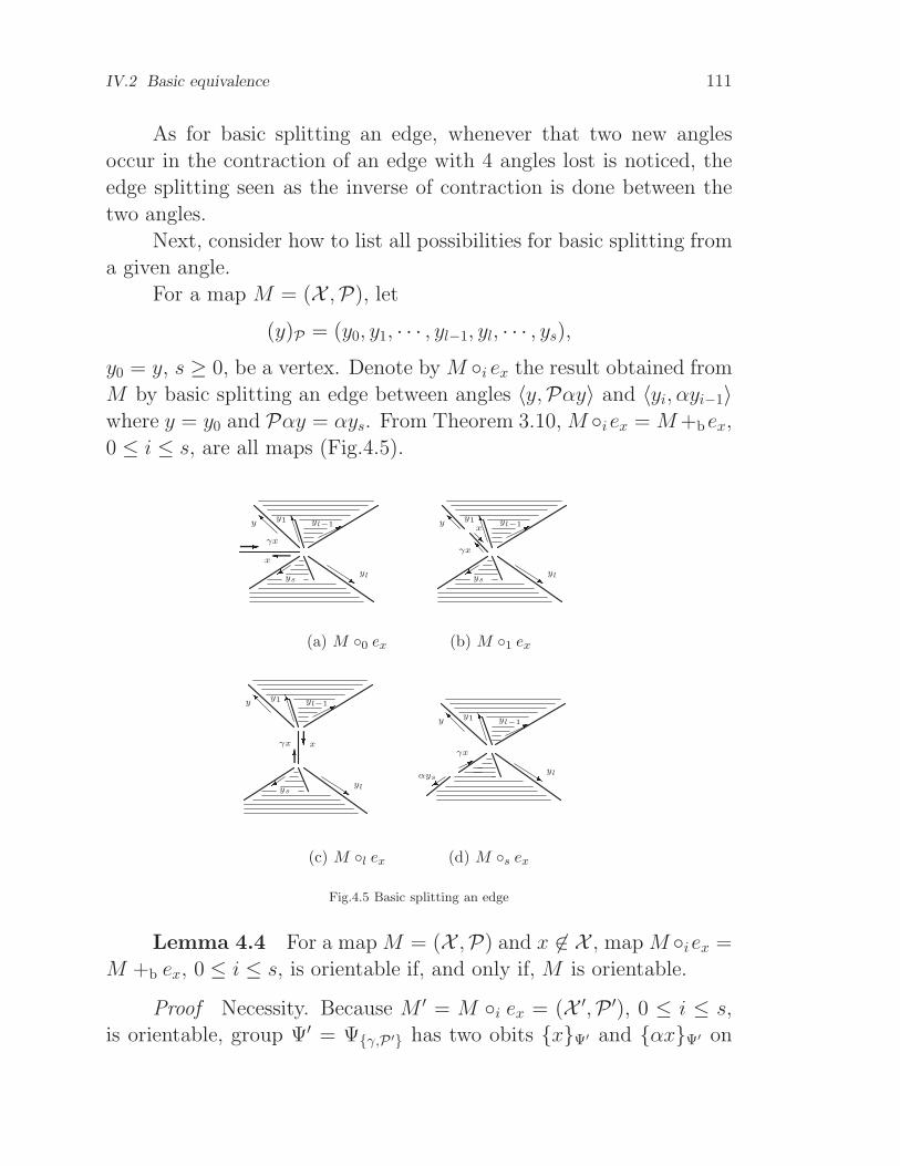
IV.2 Basic equivalence 111
As for basic splitting an edge, whenever that two new angles
occur in the contraction of an edge with 4 angles lost is noticed, the
edge splitting seen as the inverse of contraction is done between the
two angles.
Next, consider how to list all possibilities for basic splitting from
a given angle.
For a map M = (X ,P), let
(y)P = (y0, y1, · · · , yl−1, yl, · · · , ys),
y0 = y, s ≥ 0, be a vertex. Denote by M i ex the result obtained from
M by basic splitting an edge between angles 〈y,Pαy〉 and 〈yi, αyi−1〉where y = y0 and Pαy = αys. From Theorem 3.10, M iex = M+bex,
0 ≤ i ≤ s, are all maps (Fig.4.5).I M *s+yy1
ylys
yl−1 M *s+yy1
ylys
yl−1-x
γx RII x
γx
(a) M 0 ex (b) M 1 ex
αys
I M *syy1
yl
yl−1
I M *s+yy1
ylys
yl−1?6xγx + *γx
(c) M l ex (d) M s ex
Fig.4.5 Basic splitting an edge
Lemma 4.4 For a map M = (X ,P) and x 6∈ X , map M iex =
M +b ex, 0 ≤ i ≤ s, is orientable if, and only if, M is orientable.
Proof Necessity. Because M ′ = M i ex = (X ′,P ′), 0 ≤ i ≤ s,
is orientable, group Ψ′ = Ψγ,P ′ has two obits xΨ′ and αxΨ′ on

112 Chapter IV Orientability
X ′ = X +Kx. Since ex is a single link (Fig.4.5(b), (c) and (d)), or a
double link (Fig.4.5(a) and (c)),
P ′x ∈ xΨ′ and P ′αx ∈ αxΨ′.
Therefore, group Ψ = Ψγ,P has two orbits
P ′xΨ = xΨ′ − x, γx and P ′αxΨ = αxΨ′ − αx, βxon X . This implies that M is orientable.
Sufficiency. Because ex is a single link (Fig.4.5(b), (c) and (d)),
or a double link (Fig.4.5(a) and (c)), the two orbits xΨ′ = yΨ +
x, γx and αxΨ′ = αyΨ+αx, βx of group Ψ′ on X ′ are deduced
from the two orbits yΨ and αyΨ of group Ψ on X . Therefore, M ′
is orientable .
Corollary 4.2 If M ′ is the map obtained by basic adding an
edge from mapM , thenM ′ is orientable if, and only if,M is orientable.
Proof A direct result of Lemma 4.3 and Lemma 4.4.
The operation of basic appending an edge between two successive
angles of a face in a map is also called increasing duplition (Fig.4.4(b)
and (d)), and its inverse operation, decreasing duplition. And du-
ally, the operation of basic splitting an edge is also called increasing
subdivision(Fig.4.5(b) and (d)), and its inverse operation, decreasing
subdivision.
Corollary 4.3 A premap M ′ obtained by increasing duplition,
increasing subdivision, decreasing duplition, or decreasing subdivision
from a map M is still a map with the same orientability of M .
Proof The results for decreasing duplition and decreasing sub-
division are derived from Lemma 4.2. Those for increasing duplition
and increasing subdivision are from Corollary 4.2.
If map M1 can be obtained from map M2 via a series of basic
adding and/or basic subtracting an edge, then they are called mutually
basic equivalence, denoted by M1 ∼bc M2.

IV.3 Euler characteristic 113
Theorem 4.3 If maps M1 ∼bc M2, then M1 is orientable if,
and only if, M2 is orientable.
Proof A direct result of Lemma 4.2 and Corollary 4.2.
Since ∼bc is an equivalent relation, maps are partitioned into
classes of basic equivalence, in short equivalent class. Theorem 4.3
shows that the orientability of maps is an invariant in the same equiv-
alent class.
IV.3 Euler characteristic
For a map M = (X ,P), let ν = ν(M), ǫ = ǫ(M) and φ = φ(M)
are, respectively, the order(vertex number), size(edge number) and
co-order(face number) of M , then
χ(M) = ν − ǫ+ φ (4.1)
is called the Euler characteristic of M .
Theorem 4.4 Let M∗ be the dual of a map M , then
χ(M∗) = χ(M). (4.2)
Proof Because ν(M∗) = φ(M), ǫ(M∗) = ǫ(M) and φ(M∗) =
ν(M), (4.2) is obtained from (4.1).
Lemma 4.5 For a map M = (X ,P) and an edge ex, x ∈ X ,
let M − ex and M • ex be, respectively, obtained from M by deleting
and contracting the edge ex, then
χ(M) =
χ(M − ex), if ex is single;
χ(M • ex), if ex is a link.(4.3)
Proof From Theorem 3.11 and Theorem 4.4, only necessary to
consider for one of M − ex and M • ex. Here, the former is chosen. To
prove χ(M − ex) = χ(M) for ex single.

114 Chapter IV Orientability
Because ex is single, ν(M − ex) = ν(M), ǫ(M − ex) = ǫ(M)− 1
and φ(M − ex) = φ(M)− 1. From (4.1),
χ(M − ex) = ν(M)− (ǫ(M)− 1) + (φ(M)− 1)
= ν(M)− ǫ(M) + φ(M)
= χ(M).
This is just what is wanted to get.
Corollary 4.4 For any map M , χ(M) ≤ 2.
Proof By induction on the co-order φ(M). If M has only one
face, i.e., φ(M) = 1, then
χ(M) = ν(M)− ǫ(M) + 1.
In view of the connectedness,
ǫ(M) ≥ ν(M)− 1.
In consequence,
χ(M) ≤ ν(M)− (ν(M)− 1) + 1 = 2.
Thus, the conclusion is true for φ(M) = 1.
In general, i.e., φ(M) ≥ 2. Because of the transitivity on a map,
there exists a single edge ex on M . From Lemma 4.5, M ′ = M−ex has
χ(M ′) = χ(M). Since φ(M ′) = φ(M)−1, by the induction hypothesis
χ(M ′) ≤ 2. That is χ(M) ≤ 2, the conclusion.
For an indifferent reception, because the order, size and co-order
of a map can be much greater as the map is much enlarged. The con-
clusion would be unimaginable. In fact, since the deletion od a single
edge does not change the connectivity with the Euler characteristic
unchange and the size of a connected graph is never less than its order
minus one, this conclusion becomes reasonable.
Corollary 4.5 For basic subtracting an edge ex on a map M ,
χ(M −b ex) = χ(M) and χ(M •b ex) = χ(M).

IV.3 Euler characteristic 115
Proof A direct result of Lemma 4.5.
Lemma 4.6 For a map M = (X ,P) and an edge ex, x 6∈ X , let
M + ex and M ex be obtained from M via, respectively, appending
and splitting the edge ex, then
χ(M) =
χ(M + ex), if ex is single;
χ(M ex), if ex is a link.(4.4)
Proof From Theorem 3.11 and Theorem 4.4, only necessary to
consider for one of M+ex and M ex. The former is chosen. To prove
χ(M + ex) = χ(M).
Because ex is single, then ν(M + ex) = ν(M), ǫ(M + ex) =
ǫ(M) + 1 and φ(M + ex) = φ(M) + 1. From (4.1),
χ(M + ex) = ν(M)− (ǫ(M) + 1) + (φ(M) + 1)
= ν(M)− ǫ(M) + φ(M)
= χ(M).
Therefore, the lemma is true.
Corollary 4.6 For basic adding an edge ex on a mapM , χ(M+b
ex) = χ(M) and χ(M b ex) = χ(M).
Proof A direct result of Lemma 4.6.
For a map M = (X ,P) and an edge ex, x ∈ X , let M[x] and
M[+x] be obtained from M by, respectively, increasing subdivision and
increasing duplition for edge ex, and M[•x] and M[−x], by, respectively,
decreasing subdivision and decreasing duplition for edge ex. From
Corollary 4.3, they are all maps.
Corollary 4.7 For increasing subdivision and increasing dupli-
tion,
χ(M[x]) = χ(M); χ(M[+x]) = χ(M) (4.5)
and for decreasing subdivision and decreasing duplition,
χ(M[•x]) = χ(M); χ(M[−x]) = χ(M). (4.6)

116 Chapter IV Orientability
Proof Because increasing subdivision and increasing duplition
are a special type of basic adding an edge, from Corollary 4.5, (4.5)
holds. Because decreasing subdivision and decreasing duplition are
a special type of basic subtracting an edge, from Corollary 4.6, (4.6)
holds. The corollary is obtained.
The following theorem shows that the Euler characteristic is an
invariant in the basic equivalent classes of maps.
Theorem 4.5 If maps M1 ∼bc M2, then
χ(M1) = χ(M2). (4.7)
Proof Because the basic transformation consists of basic sub-
tracting and basic adding an edge, from Corollary 4,5 and Corollary
4.6, (4.7) is obtained.
IV.4 Pattern examples
Pattern 4.1 Consider the map M = (X ,P) where X = Kx+
Ky +Kz +Ku+Kw +Kl and
P = (x, y, z)(αl, γz, βw)(βl, γy, αu)(w, γu, βx),
shown in Fig.1.13.
By deleting the single edge ex onM , letM1 = (X1,P1) = M−bex,
then X1 = Ky +Kz +Ku+Kw +Kl and
P1 = (y, z)(αl, γz, βw)(βl, γy, αu)(w, γu).
By contracting the double link ez on M1, let M2 = (X2,P2) =
M1 •b ez, then X2 = Ky +Ku+Kw +Kl and
P2 = (y, βw, αl)(βl, γy, αu)(w, γu).
By contracting the double link el on M2, let M3 = (X3,P3) =
M2 •b el, then X3 = Ky +Ku+Kw and P3 = (y, βw, γy, αu)(w, γu).

IV.4 Pattern examples 117
By contracting the double link eu on M3, let M4 = (X4,P4) =
M3 •b eu, then X4 = Ky +Kw and P4 = (y, βw, γy, αw).
Now, M4 has only one vertex and only one face and hence any
basic transformation for subtracting an edge can not be done. It is a
map on the torus (Fig.4.6).
wA A
6y
B
B
v
Fig.4.6 A map basic equivalent to M
Pattern 4.2 Again, consider the map N = (X ,Q) where X =
Kx+Ky +Kz +Ku+Kw +Kl and
Q = (x, y, z)(αl, γz, βw)(βl, βy, αu)(w, γu, βx),
as shown in Fig.1.14.
By deleting the single edge ex on M , let N1 = (X1,Q1) = N−bex,
then X1 = Ky +Kz +Ku+Kw +Kl and
Q1 = (y, z)(αl, γz, βw)(βl, βy, αu)(w, γu).
By contracting the double link ez on N1, let N2 = (X2,Q2) =
N1 •b ez, then X2 = Ky +Ku+Kw +Kl and
Q2 = (y, βw, αl)(βl, βy, αu)(w, γu).
By contracting the double link el on N2, let N3 = (X3,Q3) =
N2 •b el, then X3 = Ky +Ku+Kw and
Q3 = (y, βw, βy, αu)(w, γu).

118 Chapter IV Orientability
Finally, By contracting the double link eu on N3, let N4 =
(X4,Q4) = N3 •b eu, then X4 = Ky +Kw and Q4 = (y, βw, βy, αw).
Now, the basic transformation can not be done anymore on N4.
N4 is a map on the Klein bottle, as shown in Fig.4.7.
wA A
6y
B
?βy
B
v
Fig.4.7 A map basic equivalent to N
From the two patterns, it is seen that M4 6∼bc N4, and hence
M 6∼bc N . Although their Euler characteristic are the same, i.e.,
χ(M) = χ(M4) = 1− 2 + 1 = χ(N4) = χ(N),
their orientability are different.

Activities on Chapter IV
IV.5 Observations
O4.1 For a map M = (Xα,β,P), observe how many orbits does
the group Ψα,P have on the ground set Xα,β? What condition is it
for its transitivity.
O4.2 For a map M = (Xα,β,P), observe how many orbits does
the group Ψβ,Pγ, γ = αβ, have on the ground set Xα,β? What
condition is it for its transitivity.
O4.3 For a map M = (Xα,β,P), observe how many orbits does
the group Ψβ,P have on the ground set Xα,β? What condition is it
for its transitivity.
O4.4 For a map M = (Xα,β,P), observe how many orbits does
the group Ψα,Pγ, γ = αβ, have on the ground set Xα,β? What
condition is it for its transitivity.
O4.5 If map M = (X ,P) is orientable, is M − ex always ori-
entable for any ex, x ∈ X ? If yes, explain the reason; otherwise, by
an example.
O4.6 If map M = (X ,P) is nonorientable, is M − ex always
nonorientable for any ex, x ∈ X ? If yes, explain the reason; otherwise,
by an example.
O4.7 If map M = (X ,P) is orientable, is M • ex always ori-
entable for any ex, x ∈ X ? If yes, explain the reason; otherwise, by
an example.
O4.8 If map M = (X ,P) is nonorientable, is M • ex always

120 Activities on Chapter IV
nonorientable for any ex, x ∈ X ? If yes, explain the reason; otherwise,
by an example.
O4.9 If map M = (X ,P) is orientable, is M + ex always ori-
entable for any ex, x 6∈ X ? If yes, explain the reason; otherwise, by
an example.
O4.10 If map M = (X ,P) is nonorientable, is M + ex always
nonorientable for any ex, x 6∈ X ? If yes, explain the reason; otherwise,
by an example.
O4.11 If map M = (X ,P) is orientable, is M ex always ori-
entable for any ex, x 6∈ X ? If yes, explain the reason; otherwise, by
an example.
O4.12 If map M = (X ,P) is nonorientable, is M ex always
nonorientable for any ex, x 6∈ X ? If yes, explain the reason; otherwise,
by an example.
O4.13 Show by example that a face of an orientable map M
does not correspond to a cocycle on its dualM∗.
IV.6 Exercises
E4.1 Try to prove Lemma4.1 in three different manners.
E4.2 For a map M , prove that there exists a nonnegative inte-
ger n and basic transformations π1, π2, · · · , πn such that
M∗ =n∏
i=1
πiM (4.8)
where M∗ is the dual of M .
E4.3 For a map M = (Xα,β,P), the group Ψγ,P, γ = αβ, with
two orbits on Xα,β is known. Prove that
χ(M) = 0 (mod 2). (4.9)
E4.4 Prove that a mapM = (Xα,β,P) is nonorientable if, and

IV.6 Exercises 121
only if, there exist x, y ∈ X such that
|Ky ∩ xΨαβ,P| > 2.
E4.5 Try to prove Corollary 4.4 in two different manners.
E4.6 If a map M = (Xα,β,P) has only one face, prove that
M is nonorientable if, and only if, there exists an x ∈ X such that
αx ∈ xPγ where γ = αβ.
For a map M = (Xα,β,P), let A be the set of all orbits of P on
Xα,β. Graph GM = (V,E) where V = A and
E = (A,B)|∃ x ∈ X , x ∈ A and γx ∈ B.And, GM is called the subsidiary graph of M .
E4.7 For a map M = (Xα,β,P), prove that the group Ψαβ,Phas two orbits on Xα,β if, and only if, the subsidiary graph GM of M
has two connected components.
For a map M = (Xα,β,P), γ = αβ, let fi = (xi)Pγ, (βxi)Pγ,i = 1, 2, · · · , φ, be all the faces of M . If a set S = si|1 ≤ i ≤ φ of
orbits of permutation Pγ on Xα,β satisfies |S ∩ fi| = 1,i = 1, 2, · · · , φ,
then S ia called a face representative of M .
Let graph GS = (V,E) be with V = S as a face representative
of M and e = (s, t) ∈ E as a pair of faces s and t with an edge in
common. On E, define a weight function
w(e) =
0, there exists x ∈ s such that γx ∈ t;1, otherwise
for e = (s, t) ∈ E. And, (GS, w) is called an associate net of M .
On an associate net (GS, w), GS = (V,E), of a map M , if there
exists a label l(v) ∈ 0, 1 for vertex v ∈ V such that for any e =
(u, v) ∈ E,
l(u) + l(v) = w(e) (mod 2),
then the associate net (GS, w) is said to be balanced.
E4.8 For a map M , prove that if one of its associate nets is
balanced, then all of its associate net are balanced.

122 Activities on Chapter IV
E4.9 Prove that a map is orientable if, and only if, the map
has an associate net balanced.
For a graph G = (V,E), A ⊆ E, if V has a 2-partition, i.e.,
V = V1 ∪ V2 and V1 ∩ V2 = ∅, such that
A = (u, v) ∈ E|u ∈ V1, v ∈ V2,
then A is called a cocycle of G.
E4.10 Prove that a map M is orientable if, and only if, for a
face representative S ofM , its associate net (GS, w) has e ∈ E|w(e) =
1 as a cocycle.
E4.11 Prove that a map M has its Euler characteristic 2 if, and only if, each of its faces corresponds to a cocycle of the under
graph of its dual M∗.
IV.7 Researches
R4.1 Characterize that the under graph of a map has an super
map with its Euler characteristic 1.
R4.2 Characterize that the under graph of a map has an super
map with its Euler characteristic 0.
R4.3 For any orientable map, characterize that the under graph
of the map has an super orientable map with its Euler characteristic
0.
R4.4 For a vertex regular map and a given integer g ≤ 1, char-
acterize that the under graph of the map has a super map with its
Euler characteristic g.
R4.5 For a vertex regular orientable map and a given integer
g ≤ 0, characterize that the under graph of the map has a super map
with its Euler characteristic 2g.
A graph which has a spanning circuit ia called a Hamiltonian
graph. Such a spanning circuit is called a Hamiltonian circuit of the

IV.7 Researches 123
graph. If a map has its under graph Hamiltonian, then it is called a
Hamiltonian map.
R4.6 For a Hamiltonian map and a given integer g ≤ 1, char-
acterize that the under graph of the map has a super nonorientable
map with its Euler characteristic g.
R4.7 For a Hamiltonian map and a given integer g ≤ 0, char-
acterize that the under graph of the map has a super orientable map
with its Euler characteristic 2g.
For a vertex 3-map(or cubic map), if it has only i-face and j-face,
i 6= j, i, j ≥ 3, then it is called an (i, j)f-map.
R4.8 For a given integer g ≤ 1, determine the number of
(3, 4)f-map of order n(n ≥ 1) with Euler characteristic g.
R4.9 For a given integer g ≤ 1, determine the number of
(4, 5)f-map of order n(n ≥ 1) with Euler characteristic g.
R4.10 For a given integer g ≤ 1, determine the number of
(5, 6)f-map of order n(n ≥ 1) with Euler characteristic g.
R4.11 Given a graph G of order n(n ≥ 4), determine the con-
dition for G have a super (n− 1, n)f-map.
On a (n− 1, n)f-map of order n(n ≥ 4), let φ1 be the number of
(n− 1)-faces. If its Euler characteristic is g ≤ 1, then n and φ1 should
satisfy the following condition:
(n− 1)|(n(n− g) + φ1), (4.10)
i.e., n− 1 is a facer of n(n− g) + φ1.
R4.12 Given an integer g ≤ 1, for any positive numbers n and
φ1 satisfying (4.10), determine if there exists a (n − 1, n)f-map with
its Euler characteristic g.
Chapter V
Orientable Maps
• Any irreducible orientable map under basic subtracting edges is
defined to be a butterfly. However, an equivalent class may have
more than 1 butterflies.
• The simplified butterflies are for the standard orientable maps to
show that each equivalent class has at most 1 simplified butterfly.
• Reduced rules are for transforming a map(unnecessary to be ori-
entable) into another butterfly, if orientable, in the same equivalent
class. A basic rule is extracted for deriving all other rules.
• Principles only for orientable maps are clarified to transform any
map to a simplified butterfly in the same equivalent class. Hence,
each equivalent class has at least 1 simplified butterfly.
• Orientable genus instead of the Euler characteristic is an invariant
in an equivalent class to show that orientable genus itself determine
the equivalent class.
V.1 Butterflies
On the basis of Chapter IV, this chapter discusses orientable
maps with a standard form in each of basic equivalent classes. If an

V.1 Butterflies 125
orientable map has only one vertex and only one face, then it is called
a butterfly.
Lemma 5.1 In each of basic equivalent classes, there exists a
map with only one vertex.
Proof For a map M = (Xα,β,P), if M has at least two vertices,
from the transitive axiom, there exists an x ∈ Xα,β such that (x)P and
(γx)P, γ = αβ, determine two distinct vertices. Because ex is a link,
by basic contracting ex, M′ = M •b ex ∼bc M . Then, M ′ has one
vertex less than M does. In view of Theorem 3.10, M ′ is also a map.
If M ′ does not have only one vertex, the procedure is permitted to go
on with M ′ instead of M . By the finite recursion principle a map M ′
with only one vertex can be found such that M ′ ∼bc M . This is the
lemma.
A map with only one vertex is also called a single vertex map ,
or in brief, a petal bundle .
Lemma 5.2 In a basic equivalent class of maps, there exists a
map with only one face.
Proof For a map M = (Xα,β,P), if M has at least two faces,
from the transitive axiom, there exists an x ∈ Xα,β such that (x)Pγ and
(γx)Pγ, γ = αβ, determine two distinct faces. Because ex is single,
by basic deleting ex, M′ = M −b ex ∼bc M . Now, M ′ has one face
less than M does. From Theorem 3.10, M ′ is still a map . Thus, if
M ′ is not with only one face, this procedure is allowed to go on with
M ′ instead of M . By the finite recursion principle, a map M ′ with
only one face can be finally found such that M ′ ∼bc M . The lemma
is proved.
In fact, on the basis of Theorem 3.6, Lemma 5.1 and Lemma
5.2 are mutually dual. Furthermore, what should be noticed is the
independence of the orientability for the two lemmas.

126 Chapter V Orientable Maps
Theorem 5.1 For any orientable map M , there exists a but-
terfly H such that H ∼bc M .
Proof If M has at least two vertices, from Lemma 5.1, there
exists a single vertex map L ∼bc M . In virtue of Theorem 4.3, L is
still orientable. if L has at least two faces, from Lemma 5.2, there
exists a single face map H ∼bc L. In virtue of Theorem 4.3, H is still
orientable. Since H has, finally, both one vertex and one face, H is a
butterfly. Therefore, H ∼bc L ∼bc M . This is the theorem.
This theorem enables us only to discuss butterflies for the Basic
equivalence classes of maps without loss of generality.
V.2 Simplified butterflies
Let Ok = (Xk,Jk), k ≥ 0, where
Xk =
∅, k = 0;k∑
i=1
(Kxi +Kyi), k ≥ 1(5.1)
and
Jk =
(∅), k = 0;
(
k∏
i=1
〈xi, yi, γxi, γyi〉), k ≥ 1.(5.2)
It is east to check that all Ok, k ≥ 0, are maps. And, they are called
O-standard maps. When k = 1 and 2, O1 and O2 are, respectively
given in (a) and (b) of Fig.5.1.

V.2 Simplified butterflies 1276 -? I 6 -R?x1
y1
γx1
γy1
x1y1
γx1
γy1
x2
y2
γx2
γy2
(a) O1 (b) O2
Fig.5.1 Two O-standard maps
Note 5.1 When k = 0, O0 = (∅, ∅) is seen as the degenerate
case of a map with no edge. For example, what is obtained by basic
deleting an edge on L0 = (Kx, (x, γx)) is just O0. Usually, it is seen
as the map with only one vertex without edge, or called the trivial
map.
Lemma 5.3 For any k ≥ 0, O-standard map Ok is orientable.
Proof When k = 0, from O0 = (Kx, (x, γx))−b ex,
O0 ∼bc (Kx, (x, γx)).
Because xΨ(x,γx),γ= x, γx and αxΨ(x,γx),γ
= αx, βx are two
orbits, (Kx, (x, γx)) is orientable. In view of Theorem 4.3, O0 is ori-
entable.
For k ≥ 1, assume, by induction, that Ok−1 = (Xk−1,Jk−1) is
orientable. From (5.1) and (5.2), group ΨJk−1,γ has two orbits as
x1ΨJk−1,γ = xi, γxi|1 ≤ i ≤ k − 1and
αx1ΨJk−1,γ = αxi, βxi|1 ≤ i ≤ k − 1.For Ok = (Xk,Jk), from (5.2), Jk = (〈Jk−1〉, xk, yk, γxk, γyk). Group
ΨJk,γ has only two orbits as
x1ΨJk,γ = x1ΨJk−1,γ ∪ xk, yk, γxk, γyk= xi, γxi|1 ≤ i ≤ k − 1 ∪ xk, yk, γxk, γyk= xi, γxi|1 ≤ i ≤ k

128 Chapter V Orientable Maps
and
αx1ΨJk,γ = αx1ΨJk−1,γ ∪ αxk, αyk, βxk, βyk= αxi, βxi|1 ≤ i ≤ k − 1 ∪ αxk, αyk, βxk, βyk= αxi, βxi|1 ≤ i ≤ k.
Therefore, Ok, k ≥ 1, are all orientable.
Lemma 5.4 For any k ≥ 0, O-standard map Ok has only one
face.
Proof When k = 0, since O0 = (Kx, (x, γx))−b ex, O0 should
have one face which is composed from the two faces (x) and (αx) of
(Kx, (x, γx)). Therefore, O0 has only one face(seen as a degenerate
case because of no edge).
For any Ok = (Xk,Jk), k ≥ 1, from (5.1) and (5.2),
(x1)Jkγ = (x1, γy1, γx1, y1, · · · , xk, γyk, γxk, yk)
is a face of Ok. However, since
|x1Jkγ| =1
2|Xk|,
Ok has only this face.
From (5.2), each O-standard map has only one vertex (O0 is the
degenerate case of no incident edge). Based on the above two lemmas,
any O-standard map is a butterfly. Because of the simplicity in form
for them, they are called simplified butterflies . Since for any k ≥ 0,
simplified butterfly Ok has 2k edges, one vertex and one face, its Euler
characteristic is
χ(Ok) = 2− 2k. (5.3)
Lemma 5.5 For any two simplified butterfliesOi and Oj , i, j ≥0, Oi ∼bc Oj if, and only if, i = j.
Proof Because the sufficiency, i.e., the former Oi ∼el Oj is de-
rived from the latter i = j, is natural, only necessary to prove the
necessity.

V.2 Simplified butterflies 129
By contradiction. Suppose i 6= j, but Oi ∼bc Oj . Because of the
basic equivalence, from Theorem 4.5,
χ(Oi) = χ(Oj).
However, from (5.3) and the condition i 6= j,
χ(Oi) = 2− 2i 6= 2− 2j = χ(Oj).
This is a contradiction.
Theorem 5.2 In each of the basic equivalent classes of ori-
entable maps, there is at most one map which is a simplified butterfly.
Proof By contradiction. Suppose simplified butterflies Oi and
Oj , i 6= j, i, j ≥ 0, are in the same class. However, this is a contradic-
tion to Lemma 5.5.
In the next two sections of this chapter, it will be seen that in
each basic equivalent class of orientable maps, there is at least one
map which is a simplified butterfly.
On the basis of Theorem 4.5, two butterflies of the same size
have the same Euler characteristic. Do they all simplified butterflies?
However, the answer is negative!
Example 5.1 Observe map M = (X ,J ) where
X = Kx1 +Ky1 +Kx2 +Ky2
and
J = (x1, y1, x2, y2, γx1, γy1, γx2, γy2).
Because the face
(x1)J γ = (x1, γy1, x2, γy2, γx1, y1, γx2, y2)
has 8 elements, half the elements of ground set, M has only one face.
Hence, M is a butterfly, but not a simplified butterfly. Actually, the
simplified butterfly with the sane Euler characteristic of M is O2.

130 Chapter V Orientable Maps
V.3 Reduced rules
Although butterflies are necessary to find a representative for
each basic equivalent class of orientable maps, single vertex maps are
restricted in this section for such a classification based on Lemma 5.1.
For convenience, the basic equivalence between two maps are not
distinguished from that between their basic permutations. In other
words, (X1,P1) ∼bc (X2,P2) stands for P1 ∼bc P2.
Lemma 5.6 For a single vertex map M = (X ,J ), if
J = (R, x, γx, S)
where R and S are two linear orders on X , then
J ∼bc (R, S), (5.4)
as shown from (a) to (b) in Fig.5.2.
Proof Because J = (R, x, γx, S), (J γ)γx = J x = γx, i.e.,
(γx)Jγ = (γx) is a face. Because ex is a single edge, by basic deleting
ex on M , M ′ = M −b ex = (X −Kx,J ′), J ′ = (R, S). From M ∼bc
M ′, J ∼bc J ′ = (R, S).
This lemma enables us to transform a single vertex map into
another single vertex map with one face less in a basic equivalent
class.
+Ix
γx
S
R
S
R
(a) (b)
Fig.5.2 Reduced rule (5.4)

V.3 Reduced rules 131
x1
y1
γx1
γy16 -? Ix1
y1
γx1
γy1
A
B
CD
E i K A
D
C
B
E
(a) (b)
Fig.5.3 Reduced rule (5.5)
Lemma 5.7 For (Xα,β,J ), if J = (A, x,B, y, C, γx,D, γy, E)
where A, B, C, D and E are all linear orders on X , then
J ∼bc (A,D,C,B,E, x, y, γx, γy), (5.5)
as shown from (a) to (b) in Fig.5.3.
Proof Four steps are considered for each step as a claim.
Claim 1 J ∼bc (E,A, x, z,D, C, γx, γz, B).
Proof For the angle pair (αx,J x) and (βx,J γx) of
J = (A, x,B, y, C, γx,D, γy, E),
by basic splitting ez(a link), get
J ∼bc J1 = (D, γy, E,A, x, z)(γz, B, y, C, γx).
Then, since ey is a link, by basic contracting ey on J1, get
J1 ∼bc J2 = (E,A, x, z,D, C, γx, γz, B).
This is the conclusion of Claim 1. Here, J1 and J2 are, respectively,
shown in (a) and (b) of Fig.5.4.
Claim 2 J2 ∼bc (y, A, x, B, E, γy,D, C, γx).
Proof For the pair of angle 〈αz,J2z〉 and angle between E and
A on J2 = (E,A, x, z,D, C, γx, γz, B), by basic splitting ey(a link),
get J2 ∼bc J3 = (A, x, z, y)(γy,D, C, γx, γz, B,E). Then, since ez is
a link, by basic contracting ez on J3, get
J3 ∼bc J4 = (y, A, x, B, E, γy,D, C, γx).

132 Chapter V Orientable Maps
This is the conclusion of Claim 2. Here, J3 and J4 are, respectively,
shown in (a) and (b) of Fig.5.5.
Claim 3 J4 ∼bc (B,E, z, A, y, γz, γy,D, C).O 1^9 ?6zγz
y
γx
γy
x
BC
D
E
A
i 1-x
zγx
γz
DC
B
E
A
(a) (b)
Fig.5.4 For Claim 1>1?6? y
γy
x
z
γx
γz
A
D
CB
E
O -γx y
x
γy
A
B
E
D
C
(a) (b)
Fig.5.5 For Claim 2
?6K z+9A
B
E
D
C
A
D
-qRC
B
E
z
γz
x
γy
γx
y
z
γz
y
γy
(a) (b)
Fig.5.6 For Claim 3
Proof For the angle pair (αy,J4y) and (αJ −14 γy, γy) on J4 =

V.3 Reduced rules 133
(y, A, x, B, E, γy,D, C, γx), by basic splitting ez(a link), get
J4 ∼bc J5 = (A, x,B,E, z)(γz, γy,D, C, γx, y).
Then, since ex is a link, by basic contracting ex on J3, get
J5 ∼bc J6 = (B,E, z, A, y, γz, γy,D, C).
This is the conclusion of Claim 3. Here, J5 and J6 are, respectively,
shown in (a) and (b) of Fig.5.6.
Claim 4 J6 ∼bc (A,D,C,B,E, z, x, γz, γx).
Proof For the angle pair (αz,J6z) and (αy, γz) of
J6 = (B,E, z, A, y, γz, γy,D, C),
by basic splitting ex (a link), get
J6 ∼bc J7 = (A, y, x)(γx, γz, γy,D, C,B,E, z).
Then, since ey is a link, by basic contracting ey on J7, get
J7 ∼bc J8 = (A,D,C,B,E, z, x, γz, γx).
This is the conclusion of Claim 4. Here, J7 and J8 are, respectively,
shown in (a) and (b) of Fig.5.7.*1z 6 *A
D
C B
E
A
D
CB
E
?6x
γx
y
γz
γyz
y γzγy
z
(g) (h)
Fig.5.7 Claim 4
On the basis of the four claims above,
J ∼bc J2 ∼bc J4 ∼bc J6 ∼bc J8
= (A,D,C,B,E, x, y, γx, γy).
134 Chapter V Orientable Maps
This is (5.5).
An attention should be paid to that Lemma 5.6 and Lemma 5.7
are both valid for orientable and nonorientable maps. They are called
reduced rules for maps. More precisely, They are explained as in the
following.
Reduced rule 1 A map with its basic permutation J is basic
equivalent to what is obtained by leaving off such a successive elements
〈x, γx〉, x ∈ X , on J .
Reduced rule 2 A map with its basic permutation J in the
form as (A, x.B, y, C, γx,D, γy, E) is basic equivalent to what is ob-
tained by interchanging the linear order B between x and y and the
linear order D between γx and γy, and then leaving off x, y, γx and
γy and putting 〈x, y, γx, γy〉 behind E on J .
V.4 Orientable principles
This section is centralized on discussing the basic equivalent
classes of orientable maps. The main purpose is to extract that there
is at least one simplified butterfly in each class. From the first sec-
tion of this chapter, it is known that each class is considered for only
butterflies without loss of generality.
Theorem 5.3 For a butterfly M = (Xα,β,J ), γ = αβ, if no
x, y ∈ X exist such that J = (A, x,B, y, C, γx,D, γy, E) where A, B,
C, D and E are all linear orders on Xα,β, then
M ∼bc O0, (5.6)
i.e., the trivial map(the degenerate simplified butterfly without edge).
Proof For convenience, in a cyclic permutation J on Xα,β, if two
elements x, y ∈ Xα,β are in the form as J = (A, x,B, y, C, γx,D, γy, E),
then they are said to be interlaced; otherwise, parallel.

V.4 Orientable principles 135
Claim If any two elements are parallel on J , then there is an
element x ∈ Xα,β such that 〈x, γx〉 ⊆ J , i.e., 〈x, γx〉 is a segment of
J itself.
Proof By contradiction. If no such an elements exists on Xα,be,
then for any x1 ∈ X , there is a nonempty linear order B1 on X such
that J = (A1, x, B1, γx, C1) where A1 and C1 are some linear orders
on Xα,β . Because B1 6= ∅, for any x2 ∈ B1, on the basis of orientability
and x2 and x1 parallel, the only possibility is γx2 ∈ B1. From the
known condition, there is also a linear order B2 6= ∅ on Xα,β such that
B1 = 〈A2, x2, B2, γx2, C2〉 where A2 and C2 are segments on B1, i.e.,
some linear orders on X . Such a procedure can only go on to the
infinity. This is a contradiction to the finiteness of Xα,β. Hence, the
claim is true.
If J 6= ∅, then from the claim, there exists an element x in Jsuch that J = (A, x, γx, B). However, because (γx)Jγ = (γx) is a
face in its own right, J has to be with at least two faces. This is
a contradiction to that M = (X ,J ) is a butterfly. Hence, the only
possibility is J = ∅, i.e., (5.6) holds.
Actually, this theorem including the claim in its proof is valid for
any orientable single vertex map. Therefore, it can be seen that the
reduced rule(Lemma 5.6) and the following corollary are valid for any
map (orientable or nonorientable) as well.
Corollary 5.1 Let S = 〈A, x, γx, B〉 be a segment on a vertex
of a map M . And let M ′ be obtained from M by substituting 〈A,B〉for S and afterward deleting Kx from the ground set. Then, M ′ is a
map. And, M ′ ∼bc M .
Proof Because it is easy to check that M ′ = M −b M , from
Theorem 3.10, M ′ is a map. This is the first statement. In view of
basic deletion of an edge as a basic transformation, M ′ ∼bc M .
Corollary 5.2 Let S be a segment at a vertex of a map M .
If for each element x in S, γx is also in S and any two elements in

136 Chapter V Orientable Maps
S are not interlaced, then there exists an element y in S such that
S = 〈A, y, γy, B〉.Proof In the same way of proving Theorem 5.3, the conclusion
is soon obtained.
Theorem 5.4 In a butterfly M = (Xα,β,J ), if there are x, y ∈Xα,β such that J = (A, x,B, y, C, γx,D, γy, E), then there is an inte-
ger k ≥ 1 such that
M ∼bc Ok, (5.7)
i.e., the simplified butterfly with 2k edges.
Proof Based on Reduced rule 2(Lemma 5.7),
J ∼bc (A,D,C,B,E, x, y, γx, γy).
Let H = 〈A,D,C,B,E〉. From Corollary 5.1, assume H is not in the
form as S without loss of generality. From Corollary 5.2 and Theorem
5.3, H has two possibilities: H = ∅, or there exist two elements x1
and y1 interlaced in H.
If the former, then J ∼bc (x, y, γx, γy), i.e. , M ∼el O1. Oth-
erwise, i.e., the latter, then J = (A1, x1, B1, y1, C1, γx1, D1, γy1, E1).
An attention should be paid to that E1 = 〈F1, x, y, γx, γy〉. In this
case, from Lemma 5.7,
J ∼bc (A1, D1, C1, B1, E1, x1, y1, γx1, γy1)
= (A1, D1, C1, B1, F1, x, y, γx, γy, x1, y1, γx1, γy1).
Let H1 = 〈A1, D1, C1, B1, F1〉, then for H1 instead of H, go on
the procedure. According to the principle of finite recursion, it is only
possible to exists an integer k ≥ 1 such that (5.7) holds.
This theorem shows that each basic equivalent class of orientable
maps has at least one map which is a simplified butterfly.
By considering Theorem 5.2, each basic equivalent class of ori-
entable maps has, and only has, an integer k ≥ 0 such that the sim-
plified butterfly of size k is in the class

V.5 Orientable genus 137
V.5 Orientable genus
Although Euler characteristic of a map is an invariant for basic
transformation, a basic equivalent class of maps can not be determined
by itself. This is shown from the map M in Example 4.1 of section
IV.4 and the map N in Example 4.2 of section IV.4. They both
have the same Euler characteristic. However, they are not in the
same basic equivalent class of maps because M is orientable and N is
nonorientable.
Now, a further invariant should be considered for a class of ori-
entable maps under the basic equivalence.
Theorem 5.5 For any orientable map M = (X ,P), there has,
and only has, an integer k ≥ 0, such that its Euler characteristic is
χ(M) = 2− 2k. (5.8)
Proof From Theorem 5.1 and Theorem 4.5, only necessary to
discuss butterflies. From Theorem 5.2 and Theorem 5.4, M has, and
only has, an integer k ≥ 0, such that M ∼bc Ok. Therefore, from
(5.3),
χ(M) = 2− 2k.
This is (5.8).
Corollary 5.3 The Euler characteristic of an orientable map
M = (X ,P) is always an even number, i.e.,
χ(M) = 0 (mod 2). (5.9)
Proof A direct result of Theorem 5.5.
Since Euler characteristic is an invariant of a basic equivalent
class, the integer k in (5.8) is an invariant as well. From Theorem 5.5,
k determines a basic equivalent class for orientable maps. Since each
orientable map in the basic equivalent class determined by k can be
seen as an embedding of its under graph on the orientable surface of

138 Chapter V Orientable Maps
genus k, k is also called the genus, or more precisely, orientable genus
of the map. Of course, only an orientable map has the orientable
genus.
From what has been discussed above, it is seen that although
Euler characteristic can not determine the basic equivalent class for
all maps, the Euler characteristic can certainly determine the basic
equivalent class for orientable maps.

Activities on Chapter V
V.6 Observations
O5.1 Think, is there a butterfly which has 3 edges? Further,
is there a butterfly with some odd number of edges? If yes, provide
an example. Otherwise, explain the reason.
O5.2 Observe that any butterfly with 2 edges is a simplified
butterfly. Explain the reason.
O5.3 Provide a butterfly of at most 5 edges , which is not a
simplified butterfly.
O5.4 Observe that is there a superfluous operation among the
four operations: basic deleting, basic appending, basic contracting
and basic splitting an edge in the basic transformation for the basic
equivalence? If no, indicate the role of each of them. If yes, indicate
the superfluous operation with the why.
O5.5 Think, do some three of the four operations: basic delet-
ing, basic appending, basic contracting and basic splitting an edge in
the basic transformation determine an equivalence? If do, provide an
example. Otherwise, explain the reason.
O5.6 Among the eight operations of the above four with in-
creasing duplition, decreasing duplition, increasing subdivision and
decreasing subdivision, how many groups of these operations are there
for determining the basic equivalence.
O5.7 Can an equivalence be determined by basic deleting and
basic appending an edge? If yes, observe some of invariants under the

140 Activities on Chapter V
equivalence. Otherwise, explain the reason.
O5.8 Can an equivalence be determined by basic contracting
and basic splitting an edge? If yes, observe some of invariants under
the equivalence. Otherwise, explain the reason.
O5.9 Can an equivalence be determined by basic increasing
duplition and decreasing duplition of an edge? If yes, observe some of
invariants under the equivalence. Otherwise, explain the reason.
O5.10 Can an equivalence be determined by basic increasing
subdivision and decreasing subdivision of an edge? If yes, observe
some of invariants under the equivalence. Otherwise, explain the rea-
son.
O5.11 Can the procedure of proving Lemma 5.7 by four steps
be improved to that by three steps? If yes, provide a proof of three
steps. Otherwise, explain the why.
V.7 Exercises
E5.1 By basic deleting and basic appending an edge only, prove
(A, x,B, y, C, γx,D, γy, E)∼bc (A,D,C,B,E, x, y, γx, γy).
E5.2 Prove that a map has its orientable genus 1 if, and only
if,
M ∼bc (x, y, z, γy)(βz, βt, βx, αt).
E5.3 Provide two maps of order 3 with orientable genus 1. And,
explain they are distinct.
For a set of operations A and a set of maps B not necessary to
be closed under A, if for a map M ∈ B there is no such a map N ∈ Bof size less than the size of M that N can be obtained from M by
operations in A, then M is called irreducible under A.
E5.4 For an integer k ≥ 0, determine all the irreducible sin-
gle vertex maps of orientable genus k under basic deleting and basic
appending an edge.

V.7 Exercises 141
E5.5 For an integer n ≥ 1, determine all the irreducible ori-
entable single vertex maps of size k under basic deleting and basic
appending an edge.
E5.6 For an integer n ≥ 1, determine all the irreducible ori-
entable single vertex maps of size k under basic contracting and basic
splitting an edge.
E5.7 For an integer k ≥ 0, determine all the irreducible single
vertex maps of orientable genus k under basic contracting and basic
splitting an edge.
E5.8 Prove that a complete graph Kn of order n ≥ 3 has an
orientable single face embedding if and only if,(n−1
2
)is even.
E5.9 Prove that a complete graph Kn of order n ≥ 3 has an
orientable two face embedding if and only if,(n−1
2
)is odd.
E5.10 Prove that a complete bipartite graph Km,n of order n+
m ≥ 3 has an orientable single face embedding if, and only if, (m −1)(n− 1) is even.
E5.11 Prove that a complete bipartite graph Km,n of order n+
m ≥ 3 has an orientable two face embedding if, and only if, (m −1)(n− 1) is odd.
An n-cube is the graph formed by the skeleton of the n-dimensional
cuboid. The order of an n-cube is 2n and the size, n2n−1.
E5.12 Prove that any n-cube, n ≥ 2, has an two face embed-
ding.
A map of orientable genus 0 is also said to be planar.
E5.13 Prove that a map M is planar if, and only if, each face
of M corresponds to a cocycle(See 1.6) in the under graph G(M∗) of
its dual M∗.
E5.14 Prove that a map M = (Xα,β,P) is orientable if, and

142 Activities on Chapter V
only if, P can be transformed into cyclic permutation J such that
J = (k∏
i=1
〈xi, yi〉,k∏
i=1
〈γxi, γyi〉). (5.10)
V.8 Researches
If the travel formed by a face in a map can be partitioned into
tours (travel without edge repetition), then the face is said to be pan-
tour. A map with all of its faces pan-tour is called a pan-tour map .
Because any tour can be partitioned into circuits, a pan-tour map is,
in fact, a favorable map as mentioned in 2.8. A pre-proper embedding
corresponds to what is called a tour map because each face forms a
tour in its under graph.
R5.1 Characterize and recognize that a graph has a super map
which is an orientable pan-tour map.
R5.2 Characterize and recognize that a graph has a super map
which is an orientable tour map.
R5.3 Orientable pan-tour conjecture. Prove, or improve, that
any nonseparable graph has a super map which is an orientable pan-
tour map.
R5.4 Orientable tour conjecture. Prove, or improve, that any
nonseparable graph has a super map which is an orientable tour map.
R5.5 Characterize and recognize that a graph has a super map
which is an orientable pre-proper map.
R5.6 Orientable proper map conjecture. Prove, or improve,
that any nonseparable graph has a super map which is an orientable
proper map.
The orientable minimum pan-tour genus , usually called ori-
entable pan-tour genus, of a graph is the minimum among all orientable
genera of its super pan-tour maps. Similarly, the orientable pan-tour

V.8 Researches 143
maximum genus of a graph is the maximum among all orientable gen-
era of its super pan-tour maps.
R5.7 Determine the orientable maximum pan-tour genus of a
graph.
R5.8 Determine the orientable maximum tour genus of a graph.
R5.9 Determine the orientable pan-tour genus of a graph.
R5.10 Determine the orientable tour genus of a graph.
Although many progresses has been made on determining the
orientable maximum genus of a graph, the study on determining ori-
entable (maximum) pan-tour genus, or orientable (maximum) tour
genus of a graph does not lead to any notable result yet. This sug-
gests to investigate their bounds(upper or lower) for some class of
graphs.
R5.11 Characterize the class of graphs in which each graph
has its orientable maximum pan-tour genus equal to its orientable
maximum genus. Find the least upper bound of the absolute difference
between the orientable maximum pan-tour genus and the orientable
maximum genus for a class of graphs with the two genera not equal.
R5.12 Characterize the class of graphs in which each graph has
its orientable maximum tour genus equal to its orientable maximum
genus. Find the least upper bound of the absolute difference between
the orientable maximum pan-tour genus and the orientable maximum
genus for a class of graphs with the two genera not equal.
R5.13 Characterize the class of graphs in which each graph has
its orientable pan-tour genus equal to its orientable genus. Find the
least upper bound of the absolute difference between the orientable
pan-tour genus and the orientable genus for a class of graphs with the
two genera not equal.
R5.14 Characterize the class of graphs in which each graph
has its orientable tour genus equal to its orientable genus. Find the
least upper bound of the absolute difference between the orientable

144 Activities on Chapter V
tour genus and the orientable genus for a class of graphs with the two
genera not equal.

Chapter VI
Nonorientable Maps
• Any irreducible nonorientable map under basic subtraction of an
edge is defined to be a barfly. However, an equivalent class may
have more than 1 barflies.
• The simplified barflies are for standard nonorientable maps to show
that each equivalent class has at most 1 simplified barfly.
• Nonorientable rules are for transforming a barfly into another barfly
in the same equivalent class. A basic rule is extracted for deriving
from one to all others.
• Principles only for nonorientable maps are clarified to transform
any nonorientable map to a simplified barfly in the same equivalent
class. Hence, each equivalent class has at least 1 simplified barfly.
• Nonorientable genus instead of the Euler characteristic is an invari-
ant in an equivalent class to show that nonorientable genus itself
determines the equivalent class.
VI.1 Barflies
This chapter concentrate on discussing the basic equivalent classes
of nonorientable maps by extracting a representative for each class.
On the basis of Lemma 5.1 and Lemma 5.2, Only maps with a single
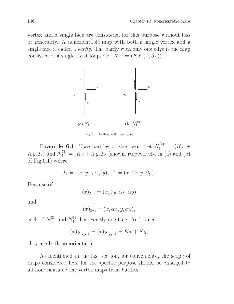
146 Chapter VI Nonorientable Maps
vertex and a single face are considered for this purpose without loss
of generality. A nonorientable map with both a single vertex and a
single face is called a barfly. The barfly with only one edge is the map
consisted of a single twist loop, i.e., N (1) = (Kx, (x, βx)).
6 -? x
y
γx
βy
6 -? x
βx
y
βy
(a) N(2)1 (b) N
(2)2
Fig.6.1 Barflies with two edges
Example 6.1 Two barflies of size two. Let N(2)1 = (Kx +
Ky, I1) and N(2)2 = (Kx+Ky, I2)(shown, respectively, in (a) and (b)
of Fig.6.1) where
I1 = (, x, y, γx, βy), I2 = (x, βx, y, βy).
Because of
(x)I1γ = (x, βy, αx, αy)
and
(x)I2γ = (x, αx, y, αy),
each of N(2)1 and N
(2)2 has exactly one face. And, since
(x)ΨI1,γ= (x)ΨI2,γ
= Kx+Ky,
they are both nonorientable.
As mentioned in the last section, for convenience, the scope of
maps considered here for the specific purpose should be enlarged to
all nonorientable one vertex maps from barflies.

VI.1 Barflies 147
Lemma 6.1 For a single vertex map M = (Xα,.be,P), M is
nonorientable if, and only if, there exists an x ∈ Xα,β such that βx ∈xP .
Proof Necessity. By contradiction. Assume that for any x ∈Xα,β, there always has γx ∈ xP , γ = αβ, then αx 6∈ xΨP,γ
. From
4.1, M is not nonorientable.
Sufficiency. Since x ∈ Xα,β and βx ∈ xP , from Corollary 4.1
and only one vertex, ΨP ,γ has only one orbit on X . Hence, M is
nonorientable.
This lemma can easily be employed for checking the nonori-
entability of a one vertex map.
Example 6.2 Six barflies of three edges. Let N(3)i = (Kx +
Ky + Kz, Ii), i = 1, 2, · · · , 6(shown, respectively, in (a,b,· · ·,f) of
Fig.6.2) whereI1 = (x, βx, y, βy, z, βz),
I2 = (x, y, z, βy, βx, βz),
I3 = (x, y, z, βz, γx, βy),
I4 = (x, βx, y, z, βz, βy),
I5 = (x, y, βx, z, βy, βz),
I6 = (x, y, z, βx, γy, γz).
Because βx ∈ xIi⊆ xΨIi,γ
, γ = αβ, i = 1, 2, · · · , 6, from Lemma
6.1, they are all nonorientable. Since
(x)I1γ = (x, αx, y, αy, z, αz),
(x)I2γ = (x, γy, z, γx, y, αz),
(x)I3γ = (x, βy, αx, γz, βz, αy),
(x)I4γ = (x, αx, y, γz, βz, αy),
(x)I5γ = (x, αy, βz, , γx, y, αz),
(x)I6γ = (x, αz, βy, αx, γy, z),
the maps (Kx + Ky + Kz, Ii), i = 1, 2, · · · , 6, are all with only one
face. Therefore, they are all barflies.

148 Chapter VI Nonorientable Maps
Theorem 6.1 For any nonorientable map M , there exists a
barfly N such that
M ∼bc N. (6.1)6 *j?Y 6 *j?Yx
βx
y
βy
z
βz
x
y
z
βy
βx
βz
(a) N(3)1 (b) N
(3)26 *j?Y 6 *j?Y
x
y
z
βz
γx
βy
x
βx
y
z
βz
βy
(c) N(3)3 (d) N
(3)46 *j?Y 6 *j?Yx
y
βx
z
βy
βz
x
y
z
βx
γy
γz
(e) N(3)5 (f) N
(3)6
Fig.6.2 Barflies of three edges
Proof From Lemma 5.1, by basic transformation M can be
transformed into a single vertex map. From Theorem 4.3, in view of

VI.2 Simplified barflies 149
the nonorientability of M , the single vertex map is also nonorientable.
Then from Lemma 5.2, by basic transformation the single vertex can
be transformed into a single face map. From Theorem 4.3, this map
is also nonorientable and hence a barfly N which satisfies(6.1).
This theorem enables us to restrict ourselves only to transform a
barfly into another barfly under the basic equivalence.
VI.2 Simplified barflies
Let Ql = (Xl, Il), l ≥ 1, where
Xl =l∑
i=1
Kxi, (6.2)
and
Il = (l∏
i=1
〈xi, βxi〉), (6.3)
they are called N -standard map . When k = 1, 2, 3 and 4, Q1 = N (1),
Q2 = N(2)2 , Q3 = N
(3)1 and Q4 are, respectively, shown in (a), (b), (c)
and (d) of Fig.6.3.
Lemma 6.2 For any l ≥ 1, N -standard maps Ql are all nonori-
entable.
Proof Because all Ql, l ≥ 1, are single vertex map and βx1 ∈x1Il
, l ≥ 1, from Lemma 6.1, they are all nonorientable.
Lemma 6.3 For any l ≥ 1, N -standard maps Ql are all with
only one face.
Proof Because Q1 = N (1), Q2 = N(2)2 and Q3 = N
(3)1 , from
the two examples above, they are all with only one face. Their faces
are (x1)I1γ = (x1, αx1), (x1)I2γ = (〈x1〉I1γ, x2, αx2) = (x1, αx1, x2, αx2)
and (x1)I3γ = (〈x1〉I2γ, x3, αx3) = (x1, αx1, x2, αx2, x3, αx3).

150 Chapter VI Nonorientable Maps
Assume, by induction, that
(x1)Il−1γ = (x1, αx1, x2, αx2, · · · , xl−1, αxl−1),
for l ≥ 4. Since Il = (〈x1〉Il−1, xl, βxl),
(x1)Ilγ = (〈x1〉Il−1γ, (Ilγ)αxl−1, · · ·).
And since (Ilγ)αxl−1 = Ilβxl−1 = xl, (Ilγ)xl = Ilα(βxl) = αxl and
(Ilγ)αxl = Ilβxl = x1,
(x1)Ilγ = (〈x1〉Il−1γ, xl, αxl)
= (x1, αx1, · · · , xl−1, αxl−1, xl, αxl).
Therefore, all N -standard maps are with only one face.
6?x1
βx1
6 -? x1
βx1
x2
βx2
(a) N1 (b) N2
6? I 6 -R?x1 *βx1j x1
βx1
x2
βx2
x3
βx3
x4
βx4+i x2
βx2
x3
βx3
(c) N3 (d) N4
Fig.6.3 Simplified barfly
VI.3 Nonorientable rules 151
Because each N -standard map has only one face, from the two
lemmas above, it is known that for any N -standard map is a barfly.
And because each of such barflies has a simpler form, it is called a
simplified barfly.
Since for any l ≥ 1, the simplified barfly Ql is with l edges, 1
vertex and 1 face, its Euler characteristic is
χ(Ql) = 2− l. (6.4)
Theorem 6.2 For any basic equivalent class of nonorientable
maps, there exists at most one map which is a simplified barfly.
Proof By contradiction. Assume that there are two simplified
barflies Qi and Qj, i 6= j, i, j ≥ 1, in a basic equivalent class of
nonorientable maps. From Theorem 4.5 and (6.4),
χ(Qi) = 2− i = 2− j = χ(Qj).
This implies i = j. A contradiction to the assumption.
In the following sections, it will be shown that there exists at
least one map which is a simplified barfly in each basic equivalent
class of nonorientable maps.
VI.3 Nonorientable rules
As mentioned above, this section is for establishing two basic
rules of transforming a nonorientable single vertex map into another
nonorientable single vertex map within basic equivalence.
Lemma 6.4 For a nonorientable single vertex mapM = (Xα,β, I),if I = (A, x,B, βx, C) where A, B and C are segments of linear order
in the cycle I on Xα,β, then
I ∼bc (A, αB−1, C, x, βx). (6.5)
Note 6.1 For a segment B = 〈Ix, I2x, · · ·, Isx〉, βx = Is+1x,

152 Chapter VI Nonorientable Maps
of linear order in the cycle of I on Iα,β, from Theorem 2.3,
〈αIsx, I(αIsx), · · · , Is−1(αIsx)〉= 〈αIsx, αIs−1x, · · · , αIx〉= αB−1.
(6.6)
Proof Two steps expressed by claims are considered for trans-
forming a nonorientable single vertex map into another nonorientable
single vertex map under the basic equivalence.
Claim 1 (A, x,B, βx, C) ∼bc (A, αB−1, βy, αC−1, y).
Proof By basic splitting an edge ey between the two angles
〈αx, Ix〉 and 〈C,A〉(i.e., the angle between C and A) on I = (A, x,B,
βx, C),I ∼bc (A, x, y)(γy, B, βx, C)
= (A, x, y)(βy, αC−1, γx, αB−1)
= (y, A, x)(γx, αB−1, βy, αC−1),
as shown in (a) and (b) of Fig.6.4.
Because ex is a link in I1 = (y, A, x)(γx, αB−1, βy, αC−1), by
basic contracting ex,
I1 ∼bc (y, A, αB−1, βy, αC−1)
= (A, αB−1, βy, αC−1, y),
as shown in (c) of Fig.6.4.
Claim 2 I2 ∼bc (A, αB−1, C, βx, x) where
I2 = (A, αB−1, βy, αC−1, y).
Proof By basic splitting ex between the two angles (γy, I2βy)
and (αy, I2y) on (A, αB−1, βy, αC−1, y),
I2 ∼bc (A, αB−1, βy, x)(γx, αC−1, y)
= (A, αB−1, βy, x)(αy, C, βx)
= (x,A, αB−1, βy)(αy, C, βx),

VI.3 Nonorientable rules 153
as shown in (d) and (e) of Fig.6.4.
Because ey is a link in I3 = (x,A, αB−1, βy)(αy, C, βx), by basic
contracting ey,
I3 ∼bc (x,A, αB−1, C, βx)
= (A, αB−1, C, βx, x),
as shown in (f) of Fig.6.4.
From Claim 1 and Claim 2,
I ∼bc I1 ∼bc I2 ∼bc I3
∼bc (A, αB−1, C, βx, x).
This is (6.5).
On the basis of the procedure in the proof of the lemma, the two
claims show the following rules as basic equivalent transformations.
Nonorientable rule 1 On a nonorientable mapM = (Xα,β,P)
unnecessary to have a single vertex, if βx ∈ (x)P, then the map M ′
obtained by translating x and βx in a direction via, respectively, seg-
ments C and D, and then by substituting αC−1 and αD−1 for, respec-
tively, C(without βx) and D(without x) on (x)P is basic equivalent to
M , i.e., M ′ ∼bc M . -?6?A
BC
? 6?A
αB−1αC−1
x
yγy
βx
xy
γx
βy
(a) (b)

154 Chapter VI Nonorientable Maps
RA
αB−1
αC−1
βy
y ?6 jA
αB−1
αC−1
βy
xγx
y
(c) (d)
?6s- ? ~A
αB−1
C
A
αB−1
C
βxx
xβy
αy
βx
(e) (f)
Fig.6.4 Claim 1 and Claim 2
This is, in fact, the Claim 1 above. However, from the proof of
Claim 2 a much simpler rule can be extracted.
Nonorientable rule 2 On a nonorientable map M = (X ,P)
unnecessary to have a single vertex, if βx ∈ (x)P, then the map M ′
obtained by translating x(or βx) via a segment C, and then by sub-
stituting αC−1 for C without βx(or x) on (x)P is basic equivalent to
M , i.e., M ′ ∼bc M .
It is seen that Nonorientable rule 1 can be done by employing
Nonorientable rule 2 twice. Therefore, Nonorientable rule 2 is funda-
mental. From this point of view, the proof of Lemma 6.4 can be done
only by Nonorientable rule 2.
Lemma 6.5 For a nonorientable single vertex map (Xα,β, I),
VI.3 Nonorientable rules 155
γ = αβ, if
I = (A, x, βx, y, z, γy, γz)
where A is a segment of linear order on Xα,β, then
I ∼ (A, x, βx, y, βy, z, βz). (6.7)
Proof By basic splitting et between the two angles (αx, βx) and
(αz, γy) on (A, x, βx, y, z, γy, γz),
I = (A, x, βx, y, z, γy, γz)
∼bc (γy, γz, A, x, t)(γt, βx, y, z)
= (γy, γz, A, x, t)(γx, βt, αz, αy)
= (t, γy, γz, A, x)(γx, βt, αz, αy).
Because ex is a link in I1 = (t, γy, γz, A, x)(γx, βt, αz, αy), by con-
tracting ex,I1 ∼bc (t, γy, γz, A, βt, αz, αy)
= (A, βt, αz, αy, t, γy, γz).
By substituting 〈A, βt〉, 〈αy, t, γy〉 and 〈∅〉 for , respectively, A, B and
C in (6.5),
I1 ∼bc (A, βt, βy, αt, y, z, βz).
Further, by substituting 〈A, βt〉, 〈αt〉 and 〈z, βz〉 for, respectively, A,
B and C in (6.5),
I1 ∼bc (A, t, βt, y, βy, z, βz)
= (A, x, βx, y, βy, z, βz).
This is (6.7).
This lemma shows that in a map M = (Xα,β,P), γ = αβ, if
(x)P = (x, βx, y, z, γy, γz, A),
then the map obtained by substituting 〈y, βy, z, βz〉 for 〈y, z, γy, γz〉on (x)P is basic equivalent to M , i.e., M ′ ∼bc M . This is usually
called nonorientable rule 3.

156 Chapter VI Nonorientable Maps
Actually, nonorientable rule 3 can be also deduced from Nonori-
entable rule 2. Although Nonorientable rule 2 is fundamental, Nonori-
entable rule 1 and nonorientable rule 3 are more convenient for recur-
sion.
VI.4 Nonorientable principles
In this section, barflies are only considered for this classification
because it has been known that there is no loss of generality for general
nonorientable maps.
Lemma 6.6 In a barfly N = (Xα,β, I), there exists an element
x ∈ Xα,β such that
I = (A, x,B, βx, C), (6.8)
where A, B and C are segments of I on Xα,β.
Proof By contradiction. Since A, B and C are permitted to
be empty, if no x ∈ X such that I satisfies (6.8), then from only one
vertex, for any x ∈ X , it is only possible that γx ∈ (x)I and βx 6∈ (x)I.Therefore, (x)ΨI,γ
and (βx)ΨI,γare the two orbits of ΨI,γ on Xα,β.
Thus, M is orientable. This is a contradiction to the nonorientability
of a barfly.
Theorem 6.3 For any barfly N = (Xα,β, I), there exists an
integer l ≥ 1 such that
I ∼bc Ql. (6.9)
Proof From Lemma 6.6 and Lemma 6.4, it can assumed that
I ∼bc (A,i∏
j=1
〈xj, βxj〉),
where i is as great as possible in this form. Naturally, i ≥ 1.
From the maximality of i and only one vertex, x ∈ A if, and only
if, γx ∈ A.
VI.5 Nonorientable genus 157
Two cases have to be discussed.
Case 1 If no element in A is interlaced, then from Corollary
5.2 and Corollary 5.1, (6.9) holds. Here, l = i.
Case 2 Otherwise, by Lemma 5.7(the reduced rule). it can be
assumed that
I ∼bc (B,
i∏
j=1
〈xj, βxj〉t∏
j=1
〈yj , zj, γyj, γzj〉),
where t is as great as possible in this form. Naturally, t ≥ 1. From
the maximality of t, no element in B is interlaced. By Corollary 5.2
and Corollary 5.1,
I ∼bc (i∏
j=1
〈xj, βxj〉t∏
j=1
〈yj , zj, γyj, γzj〉).
By nonorientable rule 3,
I ∼bc (2t+i∏
j=1
〈xj, βxj〉) = Il.
From (6.2) and (6.3), this is (6.9) where l = 2t+ i.
On the basis of Theorem 6.1 and Theorem 6.3, it is know that
there is at least one simplified barfly in each of basic equivalent classes
for nonorientable maps.
VI.5 Nonorientable genus
Now, let us go back to general nonorientable maps for the in-
variants of determining the basic equivalent classes for nonorientable
maps.
Theorem 6.4 For any nonorientable map N = (X ,P) in a
basic equivalent class, there has, and only has, an integer l ≥ 1 such
that the Euler characteristic
χ(N) = 2− l. (6.10)
158 Chapter VI Nonorientable Maps
Proof From Theorem 6.3, there is a simplified barfly in a basic
equivalent class of barflies. From Theorem 6.1, in each basic equivalent
class of nonorientable maps, there has an integer l ≥ 1 such that Ql is
in this class. On the other hand, from Theorem 6.2, only Ql is in this
class. Therefore, from (6.4) and Theorem 4.5, (6.10) is obtained.
This integer l = 2− χ(N) ≥ 1 is called the nonorientable genus
of the class N is in, or of N .
Now, it is seen from Chapters IV, V and VI that if the orientabil-
ity of a map is defined to be 1, when the map is orientable; −1, when
the map is nonorientable, then the relative genus of a map is the prod-
uct of its orientability and its absolute genus (orientable genus, if the
map is orientable; nonorientable genus, if the map is nonorientable).
Thus, a basic equivalent class of maps(orientable and nonorientable)
is determined by only its relative genus.

Activities on Chapter VI
V.6 Observations
O6.1 Think, is the map obtained by deleting an edge on a
nonorientable map still nonorientable? If yes, explain the reason. Oth-
erwise, provide an example.
O6.2 Think, the absolute genus of a map obtained via deleting
an edge on a map(orientable and nonorientable) is at most 1 less than
that of the original map. Explain the why.
O6.3 Think, is the map obtained by contracting an edge on
a nonorientable map still nonorientable? If yes, explain the reason.
Otherwise, provide an example.
O6.4 Think, the absolute genus of the map obtained via con-
tracting an edge on a map(orientable and nonorientable) is at most 1
less than that of the original map. Explain the why.
O6.5 Observe if a nonorientable map can always be trans-
formed into a barfly via only basic deleting and basic appending an
edge. If it can, explain the reason. Otherwise, discuss what type of
nonorientable maps can be done.
O6.6 Observe if a nonorientable map can always be trans-
formed into a barfly via only basic contracting and basic splitting
an edge. If it can, explain the reason. Otherwise, discuss what type
of nonorientable maps can be done.
O6.7 Observe if there are other standard maps than simpli-
fied barflies for the classification of nonorientable maps under basic

160 Activities on Chapter VI
equivalence.
O6.8 Consider how to derive the nonorientable rule 3 only from
the nonorientable rule 2.
O6.9 For a map M = (Xα,β,P), if the linear order
〈A, x,B, βx, C〉 ⊆ (x)P
is replaced by 〈A, αB−1, C, x, βx〉 to transform the permutation P on
Xα,β into permutation P ′ on Xα,β, then M ′ = (X ,P ′) is also a map.
Is M ′ basic equivalent to M? If yes, explain the reason. Otherwise,
provide an example.
O6.10 Observe that all the nonorientable rules 1–3 are valid
for any nonorientable map not necessary to be of single vertex.
VI.7 Exercises
E6.1 By basic deleting and basic appending edge, prove that
(A, x,B, αx, C) ∼bc (A, x,B, βC−1, αx).
E6.2 For a given nonorientable map M = (Xα,β,P) and an
element x ∈ Xα,β, the linear order 〈x, y, γ, γy〉 ⊆ (x)P is replaced
by 〈x, βx, y, βy〉 ⊆ (x)P ′ for obtaining M ′ = (X ,P ′). Prove that
M ′ ∼bc M .
E6.3 By basic deleting and basic appending an edge, prove
(A, x, y, γx, γy, z, αz) ∼bc (A, x, αx, y, αy, z, αz).
E6.4 List all barflies of three edges rather than those in Exam-
ple 2.
E6.5 Prove that for any two barflies, one can always be trans-
formed into another only by the nonorientable rule 2.
The irreducibility appearing in what follows is in agreement with
that in section V.7.

VI.7 Exercises 161
E6.6 Determine all irreducible barflies under the basic deleting
and basic appending an edge.
E6.7 For a given integer l ≥ 1, determine all the irreducible
maps of absolute genus l under the basic deleting and basic appending
an edge.
E6.8 Determine all irreducible barflies under the basic con-
tracting and basic splitting an edge.
E6.9 For a given integer l ≥ 1, determine all the irreducible
maps of absolute genus l under the basic contracting and basic split-
ting an edge.
E6.10 Prove that for any nonorientable map M = (Xα,β,P),
there has, and only has, an integer l ≥ 1 such that
P ∼bc
(s∏
i=1
〈xi, yi, βxi, γyi〉, xs+1, βxs+1), l = 2s+ 1, s ≥ 0;
(
s∏
i=1
〈xi, yi, βxi, γyi〉), l = 2s, s ≥ 1.
(6.11)
Here, when s = 0,s∏
i=1
〈xi, yi, βxi, γyi〉 = ∅.
E6.11 Prove that for any nonorientable map M = (Xα,β,P),
there has, and only has, an integer l ≥ 1 such that
P ∼bc (x1, x2, · · · , xk, βxk, · · · , βx2, βx1)
= (k∏
i=1
xi,1∏
i=k
βxi)
by the nonorientable rules instead of Lemma 6.4.
E6.12 Prove that for any graph G, but a tree, G has its maxi-
mum nonorientable genus
lM(G) = ǫ(G)− ν(G) + 1 (6.12)
162 Activities on Chapter VI
where ǫ(G) and ν(G) are, respectively, the size(edge number) and the
order(vertex number) of G.
VI.8 Researches
Similarly to Chapter V, among all nonorientable embeddings of
a graph, the one with minimum (maximum) of absolute genus is called
a minimum (maximum) genus embedding.
The genus of a minimum(maximum) genus embedding on nonori-
entable surfaces for a graph is called the minimum (maximum) nonori-
entable genus of the graph.
The minimum nonorientable genus of a graph is also called the
nonorientable genus of the graph. If the minimum genus embedding is
a nonorientable pan-tour(favorable) map, the the genus is called the
nonorientable pan-tour(favorable) genus.
And the likes, nonorientable pan-tour maximum genus, nonori-
entable tour genus (or nonorientable preproper genus), nonorientable
tour maximum genus, etc.
R6.1 Justify and recognize if a graph has a nonorientable em-
bedding which is a pan-tour map.
R6.2 Justify and recognize if a graph has a nonorientable em-
bedding which is a tour map.
R6.3 Determine the least upper bound and the greatest lower
bound of the nonorientable pan-tour genus(or genera) for a graph(or
a set of graphs).
R6.4 Determine the least upper bound and the greatest lower
bound of the nonorientable tour genus(or genera) for a graph(or a set
of graphs).
R6.5 Determine the least upper bound and the greatest lower
bound of the nonorientable proper genus(or genera) for a graph(or a
set of graphs).
Because it looks no much possibility to get a result simple as

VI.8 Researches 163
shown in (6.12) for determining the nonorientable pan-tour maximum
genus, nonorientable tour maximum genus and nonorientable proper
maximum genus of a graph in general, only some types of graphs are
available to be considered for such kind of result.
R6.6 Determine the least upper bound and the greatest lower
bound of the nonorientable pan-tour maximum genus(or genera) for a
graph(or a set of graphs).
R6.7 Determine the least upper bound and the greatest lower
bound of the nonorientable tour maximum genus(or genera) for a
graph(or a set of graphs).
R6.8 Determine the least upper bound and the greatest lower
bound of the nonorientable proper maximum genus(or genera) for a
graph(or a set of graphs).
R6.9 Nonorientable pan-tour conjecture (prove, or disprove).
Any nonseparable graph has a nonorientable embedding which is a
pan-tour map.
R6.10 Nonorientable tour map conjecture (prove, or disprove).
Any nonseparable graph has a nonorientable embedding which is a
tour map.
R6.11 Nonorientable proper map conjecture (prove,or disprove).
Any nonseparable graph has a nonorientable embedding which is a
proper map.
R6.12 Nonorientable Small face proper map conjecture(prove,
or disprove). A nonseparable graph of order n has a nonorientable
embedding which is a proper map with n− 1 faces.

Chapter VII
Isomorphisms of Maps
• An isomorphism is defined for the classification of maps. A map is
dealt with an isomorphic class of embeddings of the under graph
of the map.
• Two maps are isomorphic if, and only if, their dual maps are iso-
morphic with the same isomorphism.
• Two types of efficient algorithms are designed for recognizing if
two maps are isomorphic.
• Primal trail codes, or dual trail codes are used for justifying the
isomorphism of two maps.
• Two pattern examples show how to to recognize and justify if two
maps are isomorphic.
VII.1 Commutativity
In view of topology, the basic equivalent classes of maps are, in
fact, a type of topological equivalent classes of 2-dimensional closed
compact manifolds without boundary, or in brief surfaces.
Two embeddings of a graph explained in Chapter I are distinct
if they are treated as 1-dimensional complexes to be non-equivalent
under a topological equivalence.
VII.1 Commutativity 165
If a map is dealt with an embedding of a graph on a surface, then
two distinct maps are, of course, distinct embeddings of their under
graph. However, the conversed case is not necessary to be true.
This Chapter is intended to introduce a type of combinatorial
equivalence which is still seen as a type of topological equivalence but
different from that for embeddings of a graph.
In general, the equivalence between two maps can be deduced
from that between two embeddings of their under graph. However,
the coversed case is not necessary to be true.
For two maps M1 = (Xα,β(X1),P1) and M2 = (Xα,β(X2),P2), if
there exists a 1–to–1 correspondence (i.e., bijection)
τ : Xα,β(X1) −→ Xα,β(X2)
between Xα,β(X1) and Xα,β(X2) such that for any x ∈ Xα,β(X1),
τ(αx) = ατ(x), τ(βx) = βτ(x), τ(P1x) = P2τ(x), (7.1)
then τ is called an isomorphism from M1 to M2.
Lemma 7.1 If τ is an isomorphism from M1 to M2, then its
inverse τ−1 exists, and τ−1 is an isomorphism from M2 to M1.
Proof Sinceτ is a bijection, τ−1 exists. And, τ−1 is also a 1–to–1
correspondence from M2 to M1. For any y ∈ Xα,β(X2), let x = τ−1y ∈Xα,β(X1). Because y = τx and τ is an isomorphism for M1 to M2,
from (7.1),
τ(αx) = αy, τ(βx) = βy, τ(P1x) = P2y.
Further, because τ−1 exists, then
τ−1(αy) = αx = α(τ−1y),
τ−1(βy) = βx = β(τ−1y),
τ−1(P2y) = P1x = P1(τ−1y).
This implies τ−1 is an isomorphism from M2 to M1.
Based on this lemma, τ , or τ−1 can be called an isomorphism
between M1 and M2.

166 Chapter VII Isomorphisms of Maps
Examle 7.1 Let M1 = (X1,P1) where
X1 = Kx1 +Ky1 +Kz1 +Ku1
and
P1 = (x1, y1, z1)(u1, γz1)(βu1, γx1)(γy1),
and M2 = (X2,P2) where
X2 = Kx2 +Ky2 +Kz1 +Ku2
and
P2 = (y2, z2, x2)(γu2, βx2)(αu2, βz2)(βy2)
as shown in Fig.7.1.
First, let τ(x1) = x2. from the first two relations in (7.1) and the
property of Klein group, if τ is an isomorphism between M1 and M2,
thenτ(αx1) = α(τx1) = αx2,
τ(βx1) = β(τx1) = βx2,
τ(γx1) = γ(τx1) = γx2,
i.e., τ(Kx1) = Kx2.
Then, from the third relation of (7.1),
τ(y1) = τ(P1x1) = P2τ(x1) = P2x2 = y2.
Thus, τ(Ky1) = Ky2. Similarly, from
τ(z1) = τ(P1y1) = P2τ(y1) = P2y2 = z2,
τ(Kz1) = Kz2, and from
τ(u1) = τ(P1γz1) = P2τ(γz1) = P2γz2 = u2,
τ(Ku1) = Ku2.
Finally, check that if the 1–to–1 correspondence τ from X1 to
X2 satisfies τP1 = P2. In fact, from the conjugate axiom, it is only
necessary to have
τP1 = (τx1, τy1, τz1)(τu1, τγz1)(τβu1, τγx1)(τγy1)
= (x2, y2, z2)(u2, γz2)(βu2, γx2)(γy2)
= (y2, z2, x2)(γu2, βx2)(αu2, βz2)(βy2)
= P2.
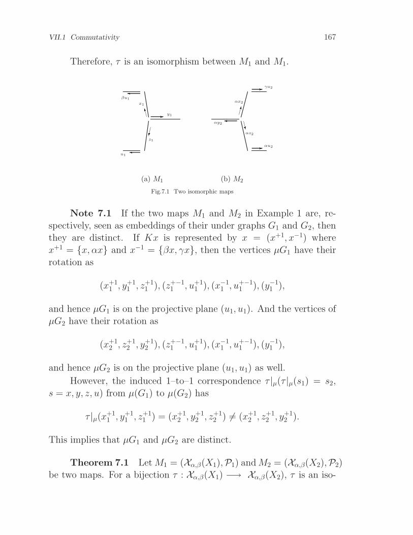
VII.1 Commutativity 167
Therefore, τ is an isomorphism between M1 and M1. O W- -
-x1
y1
z1
βu1
u1
αy2
αx2
γu2
αu2
αz2
(a) M1 (b) M2
Fig.7.1 Two isomorphic maps
Note 7.1 If the two maps M1 and M2 in Example 1 are, re-
spectively, seen as embeddings of their under graphs G1 and G2, then
they are distinct. If Kx is represented by x = (x+1, x−1) where
x+1 = x, αx and x−1 = βx, γx, then the vertices µG1 have their
rotation as
(x+11 , y+1
1 , z+11 ), (z+−1
1 , u+11 ), (x−1
1 , u+−11 ), (y−1
1 ),
and hence µG1 is on the projective plane (u1, u1). And the vertices of
µG2 have their rotation as
(x+12 , z+1
2 , y+12 ), (z+−1
1 , u+11 ), (x−1
1 , u+−11 ), (y−1
1 ),
and hence µG2 is on the projective plane (u1, u1) as well.
However, the induced 1–to–1 correspondence τ |µ(τ |µ(s1) = s2,
s = x, y, z, u) from µ(G1) to µ(G2) has
τ |µ(x+11 , y+1
1 , z+11 ) = (x+1
2 , y+12 , z+1
2 ) 6= (x+12 , z+1
2 , y+12 ).
This implies that µG1 and µG2 are distinct.
Theorem 7.1 LetM1 = (Xα,β(X1),P1) andM2 = (Xα,β(X2),P2)
be two maps. For a bijection τ : Xα,β(X1) −→ Xα,β(X2), τ is an iso-

168 Chapter VII Automorphisms of Maps
morphism if, and only if, the diagrams
Xα,β(X1)τ−−−−−−−−→ Xα,β(X2)
η1
y η2
yXα,β(X1)
τ−−−−−−−−→ Xα,β(X2)
(7.2)
for η1 = η2 = α, η1 = η2 = β, and for η1 = P1 and η2 = P2, are all
commutative , i.e., all paths with the same initial object and the same
terminal object have the same effect.
Proof Necessity. From the first relation in (7.1), for any x ∈Xα,β(X1), τ(αx) = α(τx). That is to say the result of composing the
mappings on the direct path
Xα,β(X1)α−→Xα,β(X1)
τ−→Xα,β(X2)
is the same as the result of composing the mappings on the direct path
Xα,β(X1)τ−→Xα,β(X2)
α−→Xα,β(X2).
Therefore, (7.2) is commutative for η1 = η2 = α.
Similarly, from the second and the third relations in (7.1), the
commutativity for η1 = η2 = β, and for η1 = P1 and η2 = P2 are
obtained.
Sufficiency. On the basis of (7.2), the three relations in (7.1) can
be induced from the commutativity for η1 = η2 = α, for η1 = η2 = β,
and for η1 = P1 and η2 = P2. This is the sufficiency
VII.2 Isomorphism theorem
Because the isomorphism between two maps determines an equiv-
alent relation, what has to be considered for the equivalence is the
equivalent classes, called isomorphic classes of maps. Two maps are
said to be different if they are in different isomorphic classes. In order
to clarify the isomorphic classes of maps, invariants should be inves-
tigated. In this and the next sections, a sequence of elements with

VII.2 Isomorphism theorem 169
its length half the cardinality of the ground set. In fact, this implies
that the isomorphic class can be determined by a polynomial of degree
as a linear function of half the cardinality of the ground set for both
orientable and nonorientable maps.
Lemma 7.2 If two maps M1 and M2 are isomorphic, then M1
is orientable if, and only if, M2 is orientable.
Proof Let Mi = (Xi,Pi), i = 1, 2. Assume τ is an isomorphism
from M1 to M2. From (7.2), τα = ατ ,τβ = βτ and τP1 = P2τ , i.e.,
τατ−1 = α, τβτ−1 = β and τP1τ−1 = P2.
Necessity. SinceM1 is orientable, from Theorem 4.1, permutation
group Ψ1 = ΨP1,γ has two orbits (x1)Ψ1and (αx1)Ψ1
, x1 ∈ X1 on X1.
And, since τατ−1 = α and τβτ−1 = β,
τγτ−1 = τ(αβ)τ−1 = τ(ατ−1τβ)τ−1
= (τατ−1)(τβτ−1) = αβ
= γ.
By considering τP1τ−1 = P2, for any ψ1 ∈ Ψ1,
τψ1τ−1 = ψ2 ∈ Ψ2.
Therefore, Ψ2 also has two orbits on X2, i.e., (x2)Ψ2and (αx2)Ψ2
, where
x2 = τx1 ∈ X2. This implies that M2 is orientable as well.
Sufficiency. Because of the symmetry of τ between M1 and M2,
the sufficiency is deduced from the necessity.
For a map M = (X ,P) where ν(M), ǫ(M) and φ(M) stand for,
respectively, the order(vertex number), the size(edge number) and the
coorder(face number) of M .
Lemma 7.3 If two maps M1 and M2 are isomorphic, then
ν(M1) = ν(M2), ǫ(M1) = ǫ(M2), φ(M1) = φ(M2). (7.3)
Proof Let Mi = (Xi,Pi), i = 1, 2. Assume τ is an isomorphism
from M1 to M2. From the commutativity for η1 = P1 and η2 = P2 in

170 Chapter VII Automorphisms of Maps
(7.2), τP1τ−1 = P2. Then, for any integer n ≥ 1 by induction,
τ(P1)nτ−1 = τ((P1)
n−1P1)τ−1
= τ((P1)n−1τ−1τP1)τ
−1
= (τ(P1)n−1τ−1)(τP1)τ
−1)
= (τ(P1)n−1τ−1)(τP1)τ
−1)
= (P2)n−1P2
= Pn2 .
Therefore, for any x1 ∈ X1, τx1 = x2,
τ(x1)P1= (τx1)τP1τ−1 = (x2)P2
.
Because a 1–to–1 correspondence on vertices between M1 and M2 is
induced from this, ν(M) = ν(M).
Similarly, from τγτ−1 = γ and τ(P1)nτ−1 = (P2)
n,
τ(P1γ)τ−1 = P2γ.
Further, for any integer n ≥ 1, τ(P1γ)nτ−1 = (P2γ)n. This provides
τ(x1)P1γ = (τx1)τ(P1γ)τ−1 = (x2)P2γ
as a 1–to–1 correspondence on faces between M1 and M2. Therefore,
φ(M1) = φ(M2).
Finally, from τατ−1 = α and τβτ−1 = β and hence τγτ−1 = γ,
for any x1 ∈ X1, x2 = τx1 implies τKx1 = Kx2. This provides
a 1–to–1 correspondence on edges between M1 and M2. therefore,
ǫ(M1) = ǫ(M2).
For a map M = (X ,P), the Euler characteristic given by (4.1)
is χ(M) = ν(M) − ǫ(M) + φ(M) where ν(M), ǫ(M) and φ(M) are,
respectively, the order, the size and the co-order of M .
Corollary 7.1 If two maps M1 and M2 are isomorphic, then
χ(M1) = χ(M2). (7.4)

VII.2 Isomorphism theorem 171
Proof A direct result of Lemma 7.3.
For a map M = (Xα,β,P), let M∗ = (X ∗α,β,P∗) be the dual of M .
It is, from Chapter III, known that M∗ = (Xβ,α,Pγ).
Theorem 7.2 Maps M1 and M2 are isomorphic if, and only if,
their duals M∗1 and M∗
2 are isomorphic.
Proof Let Mi = (X (i)α,β,Pi), i = 1, 2, then M∗
i = (X (i)α,β
∗,P∗i ),
i = 1, 2, where X (i)α,β
∗= X (i)
β,α and P∗i = Piγ, i = 1, 2.
Necessity. Suppose τ is an isomorphic between M1 and M2, then
from Theorem 7.1,
τατ−1 = α, τβτ−1 = β, τP1τ−1 = P2.
On the basis of this, for any x1 ∈ X (1)α,β
∗= X (1)
β,α and x2 = τx1 ∈ X (2)α,β
∗=
X (2)β,α,
τK∗x1 = τx1, βx1, αx1, γx1 = τx1, τβx1, ταx1, τγx1= x2, βx2, αx2, γx2 = K∗x2,
andτP∗1τ−1 = τ(P1γ)τ−1 = τ(P1τ
−1τγ)τ−1
= (τP1τ−1)(τγτ−1) = P2γ
= P∗2 .This implies that the diagram
X (1)α,β
∗ τ−−−−−−−−→ X (2)α,β
∗
η1
yyη2
X (1)α,β
∗ τ−−−−−−−−→ X (2)α,β
∗(7.5)
are all commutative for η1 = η2 = β, for η1 = η2 = α, and for η1 = P∗1and η2 = P∗2 . therefore, from Theorem 7.1, τ is an isomorphism
between M∗1 and M∗
2 in its own right.
Sufficiency. from the symmetry of duality, the sufficiency is de-
duced form the necessity.

172 Chapter VII Automorphisms of Maps
Let Mi = (X (i)α,β,Pi), and M∗
i = (X (i)α,β
∗,P∗i ) where X (i)
α,β
∗= X (i)
β,α
and P∗i = Piγ, i = 1, 2.
Corollary 7.2 A bijection τ : X (1)α,β −→ X
(2)α,β is an isomorphism
between maps M1 and M2 if, and only if, τ is an isomorphism between
maps M∗1 and M∗
2 .
Proof A direct result in the proof of Theorem 7.2.
VII.3 Recognition
Although some invariants are provided, they are still far from
determining an isomorphism between two maps in the last section.
In fact, it will be shown in this section that an isomorphism
between two maps can be determined by the number of invariants
dependent on their size, i.e., a sequence of invariants in a number as
a function of their size.
In order to do this, algorithms are established for justifying and
recognizing if two maps are isomorphic. In other words, an isomor-
phism can be found between two maps if any; or no isomorphism exits
at all otherwise.
Generally speaking, since the ground set of a map is finite, i.e.,
its cardinality is 4ǫ, ǫ is the size of the map, in a theoretical point of
view, there exists a permutation which corresponds to an isomorphism
among all the (4ǫ)! permutations if any, or no isomorphism at all
between two maps otherwise. However, this is a impractical way even
on a modern computer.
Our purpose is to establish an algorithm directly with the amount
of computation as small as possible without counting all the permu-
tations.
Here, two types of algorithms are presented. One is called vertex-
algorithm based on (7.2). Another is called face-algorithm based on
(7.5).
Their clue is as follows. For two maps M1 = (X1,P1) and M2 =

VII.3 Recognition 173
(X2,P2), from Lemma 7.3only necessary to consider |X1| = |X2|because the cardinality is an invariant under an isomorphism.
First, choose x1 ∈ X1 and y1 ∈ X2 (a trick should be noticed
here!).
Then, start, respectively, from x1 and y1 on M1 and M2 by a
certain rule (algorithms are distinguished by rules ). Arrange the
orbits x1ΨP1,γand y1ΨP2,γ
as cycles. If
τ(x1)ΨP1,γ= (y1)ΨP2,γ
, (7.6)
can be induced from y1 = τ(x1), then stop. Otherwise, choose another
y1(a trick!). Go no the procedure on M2 until every possible y1 has be
chosen.
Finally, if stops at the latter, then it is shown thatM1 andM2 are
not isomorphic, and denoted by M1 6= M2; otherwise, an isomorphism
between M1 and M2 is done from (7.6), denoted by M1 = M2.
Algorithm 7.1 Based on vertices, determine if two maps are
isomorphic.
Given two maps P = (X ,P) and Q = (Y ,Q), and their order,
size and co-order are all equal(otherwise, not isomorphic!). In conve-
nience, for any x ∈ X , let |x| = |xP |, i.e. , the valency of vertex
(x)P.
Initiation Given x ∈ X , choose y ∈ Y . Let τ(x) = y and
τKx = Ky. Label both x and y by 1. Naturally, Kx = Ky = K1 =
1, α1, β1, γ1 (Here, the number 1 deals with a symbol!). Label (x)Pby 0, then x = 1 is the first element coming to vertex 0. By (v, tv)
denote that tv is the first element coming to vertex v.
Let S be a sequence of symbols storing numbers and symbols and
l, the maximum of labels on all the edges with a label. Here, S = ∅,l = 1 and the minimum of labels among all labelled but not passed
vertices n = 0. If vertex (γ1)P = (1)P, the maximum vertex label
m = 0; otherwise, label vertex (γ1)P by 1m = 1.
Proceeding When all vertices are labelled as used, then go to
Halt (1).

174 Chapter VII Automorphisms of Maps
For n, let sP and sQ be, respectively, the number of edges without
label on (γtn)P and (γtn)Q.
If sP 6= sQ, when no y can be chosen, then goto Halt (2); other-
wise, choose another y and then goto Initiation.
In the direction starting from γtn, label those edges by l+1, · · · , l+s,s = sP = sQ ≥ 0 in order. Thus, two linear orders of elements with
numbers labelled
〈γtn,Pγtn, · · · ,P−1γtn〉
and
〈γtn,Qγtn, · · · ,Q−1γtn〉
are obtained.
If the two are not equal, when no y is available to choose, then
goto Halt (2); otherwise, choose another y and then goto Initiation.
Put this linear order into S as last part and then substitute the
extended sequence for S. In the meantime, label K(l + 1), K(l + 2),
· · ·, K(l + s) on P and Q. Substitute l + s for l. Mark vertex n as
used. Substitute n+ 1 for n. Let r be the number of vertices without
label in
(γ(l+ 1))P, · · · , (γ(l+ s))P ,
and label them as m + 1,· · ·,m + r in order. Substitute m + r for m.
Go on the Proceeding.
Halt (1) Output S. (2) P and Q are not isomorphic.
About Algorithm 7.1, from the way of choosing y, each element
in the ground set is passed through at most once. So there exists
a constant c such that the amount of computation is at most c|X |.Since the worst case is for y chooses all over the ground set Y ,the
total amount of computation is at most c|X |2. Because of |X | = 4ǫ
where ǫ is the size of the map, this amount is with its order as the size
squared, i.e., O(ǫ2).
As described above, if checking all possibilities of |Y|!, by Stirling

VII.3 Recognition 175
formula,
|Y|! ∼√
2πe−|Y||Y||Y|− 12
>> O(e|Y|) >> O(ǫǫ)
>> O(ǫ2)
when |Y| = |X | = 4ǫ is large enough. Thus, this algorithm is much
efficient.
Algorithm 7.2 Based on faces, determine if two maps are iso-
morphic.
Given two maps P = (Xα,β,P) and Q = (Yα,β,Q), and their
order, size and co-order are all equal(otherwise, not isomorphic!). For
convenience, let X = Xα,β, Y = Yα,β and for any x ∈ X , let |x| =
|xPγ|, i.e., the valency of face (x)Pγ where γ = αβ.
Initiation Given x ∈ X , choose y ∈ Y . Let τ(x) = y and
τKx = Ky. Label both x and y by 1. Naturally, Kx = Ky =
K1 = 1, α1, β1, γ1 (Here, the number 1 deals with a symbol!). Label
(x)P|ga by 0, then x = 1 is the first element coming to face 0. By (f, tf)
denote that tf is the first element coming to face f .
Let T be a sequence of symbols storing numbers and symbols
and l, the maximum of labels over all the edges with a label. Here,
T = ∅, l = 1 and the minimum of labels among all labelled but not
passed faces n = 0. If face (γ1)Pγ = (1)Pγ, the maximum face label
m = 0; otherwise, label face (γ1)Pγ by 1m = 1.
Proceeding When all faces are labelled as used, then go to Halt
(1).
For n, let sP and sQ be, respectively, the number of edges without
label on (γtn)Pγ and (γtn)Qγ.
If sP 6= sQ, when no y can be chosen, then goto Halt (2); other-
wise, choose another y and then goto Initiation.
In the direction starting from γtn, label those edges by l+1, · · · , l+s,s = sP = sQ ≥ 0 in order. Thus, two linear orders of elements with
numbers labelled
〈γtn,Pγγtn, · · · ,Pγ−1γtn〉

176 Chapter VII Automorphisms of Maps
and
〈γtn,Qγγtn, · · · ,Qγ−1γtn〉are obtained.
If the two are not equal, when no y is available to choose, then
goto Halt (2); otherwise, choose another y and then goto Initiation.
Put this linear order into S as last part and then substitute the
extended sequence for S. In the meantime, label K(l + 1), K(l + 1),
· · ·, K(l + s) on P and Q. Substitute l + s for l. Mark n as used.
Substitute n+ 1 for n. Let r be the number of vertices without label
in
(γ(l+ 1))P, · · · , (γ(l+ s))P ,
and label them as m + 1,· · ·,m + r in order. Substitute m + r for m.
Go on the Proceeding.
Put this linear order into T as last part and then substitute the
extended sequence for T . In the meantime, label K(l + 1), K(l + 2),
· · ·, K(l+ s) on P and Q. Substitute l+ s for l. Mark face n as used.
Substitute n+ 1 for n. Let r be the number of faces without label in
(γ(l+ 1))P, · · · , (γ(l+ s))P ,
and label them as m + 1,· · ·,m + r in order. Substitute m + r for m.
Go on the Proceeding.
Halt (1) Output T . (2) P and Q are not isomorphic.
About Algorithm 7.2, it can be seen as the dual of Algorithm
7.1. The amount of its computation is also estimated as O(ǫ2).
Note 7.2 This two algorithms suggest us that whenever a cyclic
order of edges at each vertex is given, an efficient algorithm for justi-
fying and recognizing if two graphs are isomorphic within the cyclic
order at each vertex can be established. By saying an algorithm effi-
cient, it is meant that there exists an constant c such that the amount
of its computation is about O(ǫc), ǫ is the size of the graphs.
If without considering the limitation of a cyclic order at each ver-
tex, no efficient algorithm for an isomorphism of two graphs has been

VII.4 Justification 177
found yet up to now. However, a new approach is, from what has been
discussed here, provided for further investigation of an isomorphism
between two graphs.
VII.4 Justification
In this section, it is shown that the two algorithms described in
the last section can be used for justifying and recognizing whether, or
not, two maps are isomorphic.
Lemma 7.4 Let S and T are, respectively, the outputs of Al-
gorithm 7.1 and Algorithm 7.2 at Halt (1), then
(i) Elements in S and T are all in the same orbit of group ΨP ,γon X .
(ii) S forms an orbit of group ΨP ,γ on X if, and only if, T
forms an orbit of group ΨP ,γ on X ;
(iii) S forms an orbit of group ΨP ,γ on X if, and only if, for
any x ∈ S, γx ∈ S.
Proof (i) From the proceedings of the two algorithms, it is seen
that from an element only passes through γ and P( Algorithm 7.1), or
γ and Pγ(Algorithm 7.2) for getting an element in S, or T . Because
γ,P ,Pγ ∈ ΨP ,γ and γ2 = 1 , elements in S and T are all in the same
orbit of group ΨP ,γ on X .
(ii) Necessity. Because S forms an orbit of group ΨP ,γ on X ,
and from Algorithm 7.1, S contains half the elements of X , by Lemma
4.1, group ΨP ,γ has two orbits on X . This implies in the orientable
case. Thus, from (i), T forms an orbit of group ΨP ,γ on X as well.
Sufficiency. On the basis of duality, it is deduced from the neces-
sity.
(iii) Necessity. Since S forms an orbit of group ΨP ,γ on X and
S contains only half the elements of X , by Lemma 4.1, group ΨP ,γhas two orbits on X . From the orientability, for any x ∈ S, γx ∈ S.
Sufficiency. Since for any x ∈ S, γx ∈ S, and S only contains

178 Chapter VII Automorphisms of Maps
half the elements of X , by Corollary 4.1, it is only possible that S
itself forms an orbit of group ΨP ,γ on X .
For nonorientable maps, such two algorithms have their outputs
S and T also containing half the elements of X but not forming an
orbit of group ΨP ,γ.
Lemma 7.5 Let S and T are, respectively, the outputs of Al-
gorithm 7.1 and Algorithm 7.2 at Halt (1). And , let GS and GT
be, respectively, the graphs induced by elements in S and T , then
GS = GT = G(P ).
Proof From Lemma 7.4(i), by the procedures of the two algo-
rithms, because the intersection of each of S and T with any quadricell
consists of two elements incident the two ends of the edge, S, T as
well, is incident to all edges with two ends of each edge in map P .
Therefore, GS = GT = G(P ).
Theorem 7.3 The output S of Algorithm 7.1 at Halt (1) in-
duces an isomorphism between maps P and Q. Halt (2) shows that
maps P and Q are not isomorphic.
Proof Let τ be a mapping from X to Y such that the image
and the co-image are with the same label. From the transitivity of a
map, τ is a bijection. Because τKx = Kτx, x ∈ X , then τατ−1 = α
and τβτ−1 = β. And in the Proceeding, for labelling a vertex (x)P ,τ(x)P = (τx)Q. From Lemma 7.5, this implies that τPτ−1 = Q.
Based on Theorem 7.1, τ is an isomorphism between P and Q. This
is the first statement.
By contradiction to prove the second statement. Assume that
there is an isomorphism τ between P and Q. If τ(x) = y, then by
Algorithm 7.1 the procedure should terminate at Halt (1). However,
a termination at Halt (2) shows that for any x ∈ X , there is no
elements in Y corresponding to x in an isomorphism between maps P
and Q, and hence it is impossible to terminate at Halt (1). This is a
contradiction.
VII.4 Justification 179
Therefore, the theorem is true.
Although the theorem below has its proof with a similar reason-
ing, in order to understand the precise differences the proof is still in
a detailed explanation.
Theorem 7.4 The output T of Algorithm 7.2 at Halt (1) in-
duces an isomorphism between maps P and Q. Halt (2) shows that
maps P and Q are not isomorphic.
Proof Let τ be a mapping from X to Y such that the image
and the co-image are with the same label. From the transitivity of a
map, τ is a bijection. Because τKx = Kτx, x ∈ X , then τατ−1 = α
and τβτ−1 = β. And in the Proceeding, for labelling a face (x)Pγ,
τ(x)Pγ = (τx)Qγ. From Lemma 7.5, this implies that τPγτ−1 = Qγ.
Based on Theorem 7.2, τ is an isomorphism between P and Q. This
is the first statement.
By contradiction to prove the second statement. Assume that
there is an isomorphism τ between P and Q. If τ(x) = y, then by
Algorithm 7.2 the procedure should terminate at Halt (1). However,
a termination at Halt (2) shows that for any x ∈ X , there is no
elements in Y corresponding to x in an isomorphism between maps P
and Q, and hence it is impossible to terminate at Halt (1). This is a
contradiction.
Therefore, the theorem is true.
If missing what is related to y in Algorithm 7.1 and Algorithm
7.2, then for any map M = (X ,P), the procedures will always termi-
nate at Halt (1). Thus, their outputs S and T are, respectively, called
a primal trail code and a dual trail code of M . When an element x and
a map P should be indicated, they are denoted by respective Sx(P )
and Tx(P ).
Theorem 7.5 Let P = (X ,P) and Q = (Y ,Q) be two given
maps. Then, they are isomorphic if, and only if, for any x ∈ Xchosen, there exists an element y ∈ Y such that Sx(P ) = Sy(Q), or

180 Chapter VII Automorphisms of Maps
Tx(P ) = Ty(Q).
Proof Necessity. Suppose τ is an isomorphism between maps
P = (X ,P) and Q = (Y ,Q). For the given element x ∈ X , let
y = τ(x). From Theorem 7.3, or Theorem 7.4, Sx(P ) = Sy(Q), or
Tx(P ) = Ty(Q).
Sufficiency. From Theorem 7.3, or Theorem 7.4, it is known
that by Algorithm 7.1, or Algorithm 7.2, their outputs induces an
isomorphism between P = (X ,P) and Q = (Y ,Q).
Note 7.3 In justifying whether, or not, two maps are isomor-
phic, the initial element x can be chosen arbitrarily in one of the
two maps to see if there is an element y in the other such that
Sx(P ) = Sy(Q), or Tx(P ) = Ty(Q). This enables us to do for some
convenience.
In addition, based on Theorem 7.5, all isomorphisms between
two maps can be found if any.
VII.5 Pattern examples
Here, two pattern examples are provided for further understand-
ing the procedures of the two algorithms described in the last section.
Pattern 7.1 Justify whether, or not, two maps M1 = (X1,P1)
and M2 = (X2,P2) are isomorphic where
X1 = Kx1 +Ky1, P1 = (x1, y1, βy1)(γx1)
and
X2 = Kx2 +Ky2, P2 = (y2, x2, βy2)(γx2).
First, for M1, choose x = x1. By Algorithm 7.1, find Sx(M1).
Let
P1 = (x1, y1, βy1)(γx1) = uv.

VII.5 Pattern examples 181
Initiation
x1 = 1, Kx1 = 1, α1, β1, γ1, u = 0, v = 1,
S = ∅, l = 0, m = 1.
Proceeding
Step 1 P1 = (1, y1, βy1)(γ1).
y1 = 2, Ky1 = 2, α2, β2, γ2, u = 0, v = 1,
S = 〈1, 2, β2〉, l = 2, n = 1, m = 1.
Step 2 P1 = (1, 2, β2)(γ1).
u = 0, v = 1,
S = 〈1, 2, β2, γ1〉, l = 2, n = 1, m = 1.
Halt (1) Output: Sx(M1) = S = 〈1, 2, β2, γ1〉.
Then, for M2, because a link should correspond to a link and
a vertex should correspond to a vertex with the same valency, y has
only two possibilities for choice, i.e., x2 and αx2. Choose y = x2. By
Algorithm 7.1, find Sy(M2). Let
P2 = (y2, x2, βy2)(γx2) = uv.
Initiation
x2 = 1, Kx2 = 1, α1, β1, γ1, u = 0, v = 1,
S = ∅, l = 0, m = 1.
Proceeding
Step 1 P2 = (y1, 1, βy2)(γ1).
βy2 = 2, Kβy2 = 2, α2, β2, γ2, u = 0, v = 1,
S = 〈1, 2, β2〉, l = 2, n = 1, m = 1.
Step 2 P2 = (2, 1, β2)(γ1).
u = 0, v = 1,
S = 〈1, 2, β2, γ1〉, l = 2, n = 1, m = 1.

182 Chapter VII Automorphisms of Maps
Halt (1) Output: Sy(M2) = S = 〈1, 2, β2, γ1〉.
Since Sx(M1) = Sy(M2) and y = x2, an isomorphism from M1 to
M2 is found as τ1:
τ1Kx1 = Kx2, τ1Ky1 = Ky2.
Then, choose y = αx2. By Algorithm 7.1, find Sy(M2). Let
P2 = (αx2, αy2, γy2)(βx2) = uv.
Initiation
αx2 = 1, Kαx2 = 1, α1, β1, γ1, u = 0, v = 1,
S = ∅, l = 0, m = 1.
Proceeding
Step 1 P2 = (1, αy2, γy2)(γ1).
αy2 = 2, Kαy2 = 2, α2, β2, γ2, u = 0, v = 1,
S = 〈1, 2, β2〉, l = 2, n = 1, m = 1.
Step 2 P2 = (1, 2, β2)(γ1).
u = 0, v = 1,
S = 〈1, 2, β2, γ1〉, l = 2, n = 1, m = 1.
Halt (1) Output: Sy(M2) = S = 〈1, 2, β2, γ1〉.
Since Sx(M1) = Sy(M2) and y = αx2, an isomorphism from M1
to M2 is found as τ2:
τ2Kx1 = Kαx2, τ2Ky1 = Kαy2.
In consequence, there are two isomorphisms between M1 and M2
above in all. Since 2 ∈ Sx(M1) but γ2 6∈ Sx(M1), by Lemma 7.4(iii),
M1, M2 as well, is nonorientable.
Pattern 7.2 Justify whether, or not, M1 = (X1,P1) and M2 =
(X2,P2) are isomorphic where
X1 = Kx1 +Ky1, P1 = (x1, y1, γy1)(γx1)

VII.5 Pattern examples 183
and
X2 = Kx2 +Ky2, P2 = (y2, x2, γy2)(γx2).
First, for M1, choose x = x1. By Algorithm 7.2, find Tx(M1).
Let
P1γ = (x1, γx1, y1)(γy1) = fg.
Initiation
x1 = 1, Kx1 = 1, α1, β1, γ1, f = 0, g = 1,
T = ∅, l = 0, m = 0.
Proceeding
Step 1 P1γ = (1, γ1, y1)(γy1).
y1 = 2, Ky1 = 2, α2, β2, γ2, f = 0, g = 1,
T = 〈1, γ1, 2〉, l = 2, n = 1, m = 1.
Step 2 P1γ = (1, γ1, 2)(γ2).
f = 0, g = 1,
T = 〈1, γ1, 2, γ2〉, l = 2, n = 1, m = 1.
Halt (1) Output: Tx(M1) = T = 〈1, γ1, 2, γ2〉.
Then, for M2, because a link should be corresponding to a link
and a vertex should be corresponding to a vertex with the same va-
lency, y only has two possibilities for choosing, i.e. , x2 and αx2.
Choose y = x2. By Algorithm 7.2, find Ty(M2). Let
P2γ = (x2, γx2, γy2)(y2) = fg.
Initiation
x2 = 1, Kx2 = 1, α1, β1, γ1, f = 0, g = 1,
T = ∅, l = 0, m = 0.
Proceeding
Step 1 P2γ = (1, γ1, γy2)(y2).
γy2 = 2, Kγy2 = 2, α2, β2, γ2, f = 0, g = 1,
T = 〈1, γ1, 2〉, l = 2, n = 1, m = 1.

184 Chapter VII Automorphisms of Maps
Step 2 P2γ = (1, γ1, 2)(γ2).
f = 0, g = 1,
T = 〈1, γ1, 2, γ2〉, l = 2, n = 1, m = 1.
Halt (1) Output: Ty(M2) = T = 〈1, γ1, 2, γ2〉.
Since Tx(M1) = Ty(M2) and y = x2, an isomorphism from M1 to
M2 is found as τ1:
τ1Kx1 = Kx2, τ1Ky1 = Kγy2.
Then, choose y = αx2. By Algorithm 7.2, find Ty(M2). Let
P2γ = (αx2, βx2, αy2)(βy2) = fg.
Initiation
αx2 = 1, Kαx2 = 1, α1, β1, γ1, f = 0, g = 1,
T = ∅, l = 0, m = 0.
Proceeding
Step 1 P2γ = (1, γ1, αy2)(βy2).
αy2 = 2, Kγy2 = 2, α2, β2, γ2, f = 0, g = 1,
T = 〈1, γ1, 2〉, l = 2, n = 1, m = 1.
Step 2 P2γ = (1, γ1, 2)(γ2).
f = 0, g = 1,
T = 〈1, γ1, 2, γ2〉, l = 2, n = 1, m = 1.
Halt (1) Output: Ty(M2) = T = 〈1, γ1, 2, γ2〉.
Since Tx(M1) = Ty(M2) and y = αx2, an isomorphism from M1
to M2 is found as τ2:
τ2Kx1 = Kαx2, τ2Ky1 = Kαy2.
In consequence, there are two isomorphisms between M1 and M2
in all. By Lemma 7.4(iii), M1, M2 as well, is orientable.

Activities on Chapter VII
VII.6 Observations
O7.1 Observe that whether, or not, an isomorphism between
two maps is always mapping a link to a link and a loop to a loop. If
it is, describe the reason. Otherwise, by an example.
O7.2 Observe that whether, or not, an isomorphism between
two maps is always mapping an element incident with a vertex of
valency i to an element incident with a vertex of valency i. If it is,
describe the reason. Otherwise, by an example.
O7.3 If missing τατ−1 = α or τβτ−1 = β in (7.2), whether, or
not, τ is still an isomorphism. If it is, describe the reason. Otherwise,
by an example.
O7.4 Provide two distinct embeddings of a graph which are
two isomorphic maps.
O7.5 Observe that how many non-isomorphic maps among all
embeddings of the complete graph of order 4.
O7.6 List all non-isomorphic maps of size 3 and find the dis-
tribution by relative genus.
O7.7 Explain the differences between non-isomorphic maps with
the same under graph and distinct embeddings of the graph by exam-
ples.
O7.8 Explain the differences between non-isomorphic graphs
and distinct embeddings of these graphs by examples.

186 Activities on Chapter VII
O7.9 Let τ1 and τ2 are two isomorphisms between two maps.
Observe whether, or not, their composition τ1τ−12 τ1 is also an isomor-
phism. If it is, describe the reason. Otherwise, by an example.
O7.10 Observe some algebraic properties on the set of all iso-
morphisms between two maps.
O7.11 Observe that for two maps M1 = (X1,P1) and M2 =
(X1,P2), is the composition of two permutations P1 and P2 a map? If
it is, describe the reason. Otherwise, by an example.
O7.12 Observe some algebraic properties of the sets of all maps
and premaps on the same ground set under the composition of per-
mutations.
VII.7 Exercises
If an edge is with its two ends of valencies i and j, then it is called
a (i, j)-edge, 0 ≤ i, j ≤ 2ǫ. If its two incident faces are of valencies l
and s, then it is called a (l, s)∗-edge, 0 ≤ s, t ≤ 2ǫ. Here, ǫ is the size
of a map.
E7.1 Let mij(M) and nij(M) are, respectively, the numbers of
(i, j)-edge and (i, j)∗-edge in map M . Prove that if maps M1 and M2
are isomorphic, then for any i and j, 0 ≤ i, j ≤ 2ǫ, mij(M1) = mij(M2)
and nij(M1) = nij(M2).
E7.2 Prove that a bijection between the basic sets of two maps
is an isomorphism of the two maps if, and only if, it induces both the
correspondences between their vertices and between their faces.
E7.3 Design an algorithm which is different from Algorithm 7.1
and Algorithm 7.2 for justifying an isomorphism between two maps
such that its computation amount is in the same order as their’s.
E7.4 Prove that Algorithm 7.1 and Algorithm 7.2 are with the
computation order O(ǫ) in justifying an isomorphism of two maps
which have a triangular face, or a vertex of valency 3 where ǫ is the

VII.7 Exercises 187
size of the maps.
E7.5 Prove that Algorithm 7.1 and Algorithm 7.2 are with the
computation order O(ǫ) in justifying an isomorphism of two maps
which have only one —articulate vertex(a vertex of valency 1), or only
one loop where ǫ is the size of the maps.
E7.6 Determine the number of non-isomorphic butterflies of
size m ≥ 1, or establish a method to list them.
E7.7 Determine the number of non-isomorphic barflies of size
m ≥ 1, or establish a method to list them.
E7.8 On the basis of Algorithm 7.1, design an algorithm for
justifying an isomorphism between two planar graphs(not maps!), and
estimate its computation order.
E7.9 On the basis of Algorithm 7.2, design an algorithm for
justifying an isomorphism between two planar graphs(not maps!), and
estimate its computation order.
For any map M , let T be a spanning tree of its under graph
G(M). Each co-tree edge is partitioned into two semi-edges seen as
edges. Because what is obtained is just a tree when each of such
semi-edges is seen with a new articulate vertex, it is a joint tree cor-
responding to an embedding of its under graph G(M), also called an
joint tree of M .
If x and βx are in the same direction for an edge X = Kx
partitioned along the joint tree, then it is said to be with the same
sign, denoted by X and X; otherwise, different signs, denoted by X
and X−1, or X−1 and X. The cyclic order of letters with signs of such
semi-edges partitioned into is called an joint sequence of the map.
E7.10 Prove that a graph G is planar if, and only if, there
exists an joint sequence of maps whose under graph is G such that
each letter is with different signs and no two letters are interlaced.
E7.11 Prove that for any complete graph Kn, n ≥ 1, there
is no joint tree for all maps whose under graph are Kn such that it
corresponds to a simplified butterfly.

188 Activities on Chapter VII
VII.8 Researches
R7.1 Discuss whether, or not, there exits a number, indepen-
dent on the size of a map considered, of invariants within isomorphism
of maps for justifying and recognizing an isomorphism between two
maps.
R7.2 For a given graph G and an integer g, determine the
number of distinct embeddings of G on the surface of relative genus
g, and the number of non-isomorphic maps among them.
R7.3 For a given type of graphs G and an integer g, find the
number of distinct embeddings of graphs in G on the surface of relative
genus g, and the number of non-isomorphic maps among them.
R7.4 Determine the number of non-isomorphic triangulations
of size m ≥ 3.
R7.5 Determine the number of non-isomorphic quadrangula-
tions of size m ≥ 4.
R7.6 For an integral vector (n2, n4, · · · , n2i, · · ·), find the num-
ber of non-isomorphic Euler planar maps each of which has n2i vertices
of valency 2i, i ≥ 1.
Because it can be shown that two graphs G1 and G2 are isomor-
phic if, and only if, for a surface they can be embedded into, there
exist embeddings µ1(G1) and µ2(G2) isomorphic, this enables us to
investigate the isomorphism between two graphs. The aim is at an
efficient algorithm if any.
R7.7 Suppose map M1 is an embedding of G1 on an orientable
surface of genus g, justify whether, or not, there is an embedding M2
of graph G2 such that M2 and M1 are isomorphic.
R7.8 Suppose mapM1 is an embedding ofG1 on a non-orientable
surface of genus g, justify whether, or not, there is an embedding M2
of graph G2 such that M2 and M1 are isomorphic.
R7.9 According to [Liu1], any graph with at least a circuit has
a non-orientable embedding with only one face. Justify whether, or

VII.8 Researches 189
not, two graphs G1 and G2 have two respective single face embeddings
which are isomorphic.
R7.10 Justify whether, or not, a graph has two distinct single
face embeddings which are isomorphic maps.
A graph is called up-embeddable if it has an orientable embedding
of genus which is the integral part of half the Betti number of the
graph. Because of the result in [Liu1], unnecessary to consider the
up-embeddability for non-orientable case.
R7.11 Determine the up-embeddability and the maximum ori-
entable genus of a graph via its joint sequences.
R7.12 For a given graph G and an integer g, justify whether,
or not, the graph G has an embedding of relative genus g.

Chapter VIII
Asymmetrization
• An automorphism of a map is an isomorphism from the map to
itself. All automorphisms of a map form a group called its au-
tomorphism group. of a map is, in fact, the trivialization of its
automorphism group.
• A number of sharp upper bounds of automorphism group orders
for a variety of maps are provided.
• The automorphism groups of simplified butterflies and those of
simplified barflies are determined.
• The realization of of a map is from rooting an element of the ground
set.
VIII.1 Automorphisms
An isomorphism of a map to itself is called an automorphism .
Let τ be an automorphism of map M = (X ,P). If for x ∈ X , τ(x) = y
and x 6= y, then two elements x and y play the same role on M , or
say, they are symmetric. Hence, an automorphism of a map reflects
the symmetry among elements in the ground set of the map.
Lemma 8.1 Suppose τ1 and τ2 are two automorphisms of map
M , then their composition τ1τ2 is also an automorphism of map M .

VIII.1 Automorphisms 191
Proof Because τ1 is an automorphism of M = (Xα,β,P), from
(7.2)
τ1ατ−11 = α, τ1βτ
−11 = β, τ1Pτ−1
1 = P .Similarly, for τ2,
τ2ατ−12 = α, τ2βτ
−12 = β, τ2Pτ−1
2 = P .
Therefore, for τ1τ2,
(τ1τ2)α(τ1τ2)−1 = (τ1τ2)α(τ−1
2 τ−11 )
= τ1(τ2ατ−12 )τ−1
1
= τ1ατ1 = α,
(τ1τ2)β(τ1τ2)−1 = (τ1τ2)β(τ−1
2 τ−11 )
= τ1(τ2βτ−12 )τ−1
1
= τ1βτ1 = β,
and(τ1τ2)P(τ1τ2)
−1 = (τ1τ2)P(τ−12 τ−1
1 )
= τ1(τ2Pτ−12 )τ−1
1
= τ1Pτ1 = P .This implies that for τ1τ2, (7.2) is commutative. From Theorem 7.1,
τ1τ2 is an automorphism of M as well.
On the basis of the property on permutation composition, auto-
morphisms satisfy the associate law for composition.
Because an automorphism τ is a bijection, it has a unique inverse
denoted by τ−1. Because
τ−1ατ = τ−1(τατ−1)τ = (τ−1τ)α(τ−1τ) = α,
and similarly,
τ−1βτ = β, τ−1Pτ = P ,from Theorem 7.1, τ−1 is also an automorphism.
If an element x ∈ X has τ(x) = x for a mapping(particularly, an
automorphism) τ , then x is called a fixed point of τ . If every element

192 Chapter VIII Asymmetrization
is a fixed point of τ , then τ is called an identity . Easy to see that an
identity on X is, of course, an automorphism of M , usually said to be
trivial . By the property of a permutation, an identity is the unity of
automorphisms, always denoted by 1.
In summary, the set of all automorphisms of a map M forms
a group, called the automorphism group of M , denoted by Aut(M).
Its order is the cardinality of the set aut(M) = |Aut(M)|, i.e., the
number of elements in Aut(M) because of the finiteness.
Theorem 8.1 Let τ be an automorphism of map M = (X ,P).
If τ has a fixed point, the τ = 1, i.e., the identity.
Proof Suppose x is the fixed point, i.e. , τ(x) = x. Because τ
is an isomorphism, From (7.1),
τ(αx) = ατ(x) = αx,
τ(βx) = βτ(x) = βx
τ(Px) = P(τ(x)) = Px,i.e., αx, βx and Px are all fixed points.
Then for any ψ ∈ Ψα,β,P,
τ(ψ(x)) = ψ(τ(x)) = ψ(x).
Therefore, from transitive axiom, every element on X is a fixed
point of τ . This means that τ is the identity.
In virtue of this theorem, the automorphism induced from τ(x) =
y can be represented by τ = (x→ y).
Example 8.1 Let us go back to the automorphisms of the maps
described in Pattern 7.1 and Pattern 7.2.
If M1 and M2 in Pattern 7.1 are taken to be
M = (Kx+Ky, (x, y, βy)(γx)) = M1,
then it is seen that only one nontrivial automorphism τ = (x → αx)
exists. Thus, its automorphism group is
Aut(M) = 1, (x→ αx),

VIII.2 Upper bound of group order 193
i.e., a group of order 2.
Then, maps M1 and M2 in Pattern 7.2 are taken to be
M = (Kx+Ky, (x, y, γy)(γx)) = M2,
it has also only one nontrivial automorphism τ = (x → αx). So, its
automorphism group is
Aut(M) = 1, (x→ αx),a group of order 2, as well.
However, maps M1 and M2 here are not isomorphic. In fact, it
is seen that M1 is nonorientable with relative genus −1. and M2 is
orientable of relative genus 1.
VIII.2 Upper bounds of group order
Because the automorphism group of a combinatorial structure
with finite elements is an finite permutation group in its own right, its
order must be bounded by an finite number. And, because there are
n! permutations on a combinatorial structure of n elements, the order
of its automorphism group is bounded by n!.
However, n! is an exponential function of n according to the
Stirling approximate formula, it is too large for determining the auto-
morphism group in general.
Now, it is asked that is there an constant c such that the order of
automorphism group is bounded by nc, or denoted by O(nc), if there
is, then such a result would be much hopeful for the determination of
the group efficiently.
In matter of fact, if the order of automorphism group is O(nc), c
is independent of n for a structure with n elements, then an efficient
algorithm can be designed for justifying and recognizing if two of them
are isomorphic in a theoretical point of view.
Lemma 8.2 For any map M = (X ,P), the order of its auto-
morphism group is
aut(M) ≤ |X | = 4ǫ(M) (8.1)

194 Chapter VIII Asymmetrization
where ǫ(M) = 14|X | is the size of M .
Proof From Theorem 8.1, M has at most |X | = 4ǫ(M) auto-
morphism, i.e., (8.1).
The bound presented by this lemma is sharp, i.e., it can not be
reduced any more. For an example, the link map L = (Kx, (x)(γx)).
The order of its automorphism group is 4 = |Kx| = ǫ(L).
Lemma 8.3 For an integer i ≥ 1, let νi(M) be the number of
i-vertices(vertex incident with i semi-edges) in map M = (X ,P), then
aut(M) | 2iνi(M), (8.2)
i.e., aut(M) is a factor of 2iνi(M).
Proof Let τ ∈ Aut(M) be an automorphism of M . For x ∈ X ,
(x)P is an i-vertex, assume τ(x) = y. From the third relation of
(7.1), (y)P is also an i-vertex. Then, the elements of Xi = x|∀x ∈X , |xP| = i can be classified by the equivalent relation
x ∼Aut y ⇐⇒ ∃τ ∈ Aut(M)x = τy
induced from the group Aut(M).
From Theorem 8.1, Aut(G) has a bijection with every equivalent
class. This implies that each class has aut(M) elements. Therefore,
aut(M) | |Xi|.
Because |Xi| = 2iνi(M), (8.2) is soon obtained.
This lemma allows to improve, even apparently improve the bound
presented by Lemma 8.1 for a map not vertex-regular(each vertex has
the same valency).
Lemma 8.4 For an integer j ≥ 1, let φj(M) be the number of
j-faces of map M = (X ,P), then
aut(M) | 2jφj(M), (8.3)

VIII.2 Upper bound of group order 195
i.e., aut(M) is a factor of 2jφj(M).
Proof Let τ ∈ Aut(M) be an automorphism of M . For x ∈ X ,
(x)Pγ is a j-face, assume τ(x) = y. From the first two relations of
(7.1), τ(γx) = γy. Then from this and the third relations, τ((Pγ)x) =
(Pγ)y. Thus, (y)Pγ is also a j-face. And, the elements of Xj = x|∀x ∈X , |xPγ| = j can be classified by the equivalence
x ∼Aut y ⇐⇒ ∃τ ∈ Aut(M)x = τy
induced from the group Aut(M).
Further, from Theorem 8.1, Aut(G) has a bijection with every
equivalent class. This leads that each class has aut(M) elements.
Therefore,
aut(M) | |Xj|.Because |Xj| = 2jφj(M), (8.3) is soon obtained.
This lemma allows also to improve, even apparently improve the
bound presented by Lemma 8.1 for a map not face-regular(each face
has the same valency).
Theorem 8.2 Let νi(M) and φj(M) be, respectively, the num-
bers of i-vertices and j-faces in map M = (X ,P), i, j ≥ 1, then
aut(M) | (2iνi, 2jφj | ∀i, i ≥ 1, ∀j, j ≥ 1), (8.4)
where (2iνi, 2jφj | ∀i, i ≥ 1, ∀j, j ≥ 1) represents the greatest
common divisor of all the numbers in the parentheses.
Proof From Lemma 8.3, for any integer i ≥ 1,
aut(M) | 2iνi(M).
From Lemma 8.4, for any integer j ≥ 1,
aut(M) | 2iφj(M).
By combining the two relations above, (8.4) is soon found.

196 Chapter VIII Asymmetrization
Based on this theorem, the following corollary is naturally de-
duced.
Corollary 8.1 Let νi(M) and φj(M) be, respectively, the num-
bers of i-vertices and j-faces in map M = (X ,P), i, j ≥ 1, then
aut(M) ≤ (2iνi, 2jφj | ∀i, i ≥ 1, ∀j, j ≥ 1). (8.5)
Proof A direct result of (8.4).
Corollary 8.2 For map M = (X ,P), ǫ(M) is its size, then
aut(M) | 4ǫ(M). (8.6)
Proof Because
4ǫ(M) = 2∑
i≥1
iνi(M) = 2∑
j≥1
jφj(M)
=∑
i≥1
2iνi(M) =∑
j≥1
2jφj(M),
we have
(2iνi, 2jφj | ∀i, i ≥ 1, ∀j, j ≥ 1) | 4ǫ(M).
Hence, from Theorem 8.2, (8.6) is soon derived.
VIII.3 Determination of the group
In this section, the automorphism groups of standard maps, i.e.,
simplified butterflies and simplified barflies, are discussed.
First, observe the orientable case. For
O1 = (X1,J1) = (Kx1 +Ky1, (x1, y1, γx1, γy1)),

VIII.3 Determination of the group 197
by Algorithm 7.1,
Sx1(O1) = 1, y1, γ1, γy1 = 1, 2, γ1, γ2;
Sαx1(O1) = 1, βy1, γ1, αy1 = 1, 2, γ1, γ2;
Sβx1(O1) = 1, αy1, γ1, βy1 = 1, 2, γ1, γ2;
Sγx1(O1) = 1, γy1, γ1, y1 = 1, 2, γ1, γ2;
Sy1(O1) = 1, γx1, γ1, x1 = 1, 2, γ1, γ2;
Sαy1(O1) = 1, αx1, γ1, βx1 = 1, 2, γ1, γ2;
Sβy1(O1) = 1, βx1, γ1, αx1 = 1, 2, γ1, γ2;
Sγy1(O1) = 1, x1, γ1, γx1 = 1, 2, γ1, γ2,
i.e.,
Sx1(O1) = Sαx1
(O1) = Sβx1(O1) = Sγx1
(O1) = Sy1(O1)
= Sαy1(O1) = Sβy1
(O1) = Sγy1(O1)
= 1, 2, γ1, γ2.
Thus, O1 has its automorphism group of order 8, i.e.,
aut(O1) = 4× (2× 1) = 8.
A map with a non-trivial automorphism group is said to be sym-
metrical. If a map with its automorphism group of order 4 times its
size, the it is said to be completely symmetrical. It can be seen that O1
is completely symmetrical. However, none of Ok, k ≥ 2, is completely
symmetrical although they are all symmetrical.
Theorem 8.3 For simplified butterflies(orientable standard maps)
Ok = (Xk,Jk), k ≥ 1, where
Xk =k∑
i=1
(Kxi +Kyi)
and
Jk = (
k∏
i=1
〈xi, yi, γxi, γyi〉),

198 Chapter VIII Asymmetrization
we have
aut(Ok) =
2k, if k ≥ 2;
8, if k = 1.(8.7)
Proof From the symmetry between 〈xi, yi, γxi, γyi〉, i ≥ 2, and
〈x1, y1, γx1, γy1〉 in Jk, k ≥ 2, only necessary to calculate Sx1(Ok),
Sγx1(Ok), Sy1
(Ok), Sγy1(Ok), Sαx1
(Ok), Sβx1(Ok), Sαy1
(Ok), and
Sβy1(Ok) by Algorithm 7.1.
From Algorithm 7.1,
Sx1(Ok) = 1, y1, γ1, γy1,
k∏
i=1
〈xi, yi, γxi, γyi〉
= 1, 2, γ1, γ2,
k∏
i=2
〈(2i− 1), 2i, γ(2i− 1), γ2i〉
=k∏
i=1
〈(2i− 1), 2i, γ(2i− 1), γ2i〉,
Sαx1(Ok) = 1, α(
k∏
i=1
〈xi, yi, γxi, γyi〉)−1, βy1, γ1, αy1
6= Sx1(Ok),
Sγx1(Ok) = 1, γy1,
k∏
i=1
〈xi, yi, γxi, γyi〉, γ1, y1
6= Sx1(Ok),
Sβx1(Ok) = 1, αy1, γ1, α(
k∏
i=1
〈xi, yi, γxi, γyi〉)−1, βy1
6= Sx1(Ok),
Sy1(Ok) = 1, γx1, γ1,
k∏
i=1
〈xi, yi, γxi, γyi〉, x1
6= Sx1(Ok),

VIII.3 Determination of the group 199
Sαy1(Ok) = 1, αx1, α(
k∏
i=1
〈xi, yi, γxi, γyi〉)−1, γ1, βx1
6= Sx1(Ok),
Sγy1(Ok) = 1,
k∏
i=1
〈xi, yi, γxi, γyi〉, x1, γ1, γx1
6= Sx1(Ok),
Sβy1(Ok) = 1, βx1, α1, αx1, α(
k∏
i=1
〈xi, yi, γxi, γyi〉)−1
= 1, 2.γ1, γ2,
k∏
i=2
〈(2i− 1), 2i, γ(2i− 1), γ2i〉
= Sx1(Ok).
Because two automorphisms are from Sβy1(Ok) = Sx1
(Ok), Ok
have 2× k = 2k automorphisms altogether. Hence, when k ≥ 2,
aut(Ok) = 2k.
When k = 1, aut(O1) = 8 is known.
Then, observe the nonorientable case. for
Q1 = (X1, I1) = (Kx1, (x1, βx1)),
by Algorithm 7.1,
Sx1(Q1) = 1, β1; Sαx1
(Q1) = 1, β1;
Sβx1(Q1) = 1, β1; Sγx1
(Q1) = 1, β1,
i.e., aut(Q1) = 4.
Theorem 8.4 For simplified barfliesQl = (Xl, Il), l ≥ 1, where
Xl =
l∑
i=1
Kxi

200 Chapter VIII Asymmetrization
and
Il =l∏
i=1
〈xi, βxi〉,
we have
aut(Ql) =
2l, l ≥ 2;
4, l = 1.(8.8)
Proof From the symmetry of 〈xi, βxi〉, i ≥ 2, and 〈x1, βx1〉 in
Il, l ≥ 2, only necessary to calculate
Sx1(Ql), Sαx1
(Ql), Sβx1(Ql) and Sγx1
(Ql)
by employing Algorithm 7.1.
From Algorithm 7.1,
Sx1(Ql) = 1, β1,
l∏
i=2
〈xi, βxi〉
= 1, β1, 2, β2,l∏
i=3
〈xi, βxi〉
=l∏
i=1
〈i, βi〉,
Sαx1(Ql) = 1, α(
l∏
i=2
〈xi, βxi〉)−1, β1
6= Sx1(Ql),
Sβx1(Ql) = 1,
l∏
i=2
〈xi, βxi〉, β1
6= Sx1(Ql),

VIII.4 Rootings 201
Sγx1(Ql) = 1, β1, α(
l∏
i=2
〈xi, βxi〉)−1
= 1, β1, l, βl,2∏
i=l−1
〈γxi, αxi〉
=
l∏
i=1
〈i, βi〉
= Sx1(Ql).
Because two automorphisms are from Sγx1(Ql) = Sx1
(Ql), Ql has
2× l = 2l automorphisms altogether. Hence, when l ≥ 2,
aut(Ql) = 2l.
When l = 1, aut(Q1) = 4 is known.
Similarly, the two theorems can also be proved by employing
Algorithm 7.2.
VIII.4 Rootings
For a given map M = (X ,P), if a subset R ⊆ X is chosen such
that an automorphism of M with R fixed, i.e., an element of R does
only correspond to an element of R, then M is called a set rooted map.
The subset R is called the rooted set of M , and an element of R is
called a rooted element .
Theorem 8.5 For a set rooted map MR = (X ,P), R is the
rooted set,
aut(MR) | |R|. (8.9)
Proof Assume that all elements in R are partitioned into equiv-
alent classes under the group Aut(MR). From Theorem 8.1, each class
has aut(MR) elements. Therefore, (8.9) is satisfied.

202 Chapter VIII Asymmetrization
Corollary 8.3 For a set rooted map MR = (X ,P), R is the
rooted set,
aut(MR) ≤ |R|. (8.10)
Proof A direct result of (8.9).
For a given mapM = (X ,P), if a vertex vx, x ∈ X , is chosen such
that an automorphism of M has to be with vx fixed, i.e., an element
incident with vx has to correspond to an element incident with vx, then
M is called a vertex rooted map. The vertex vx is called the rooted
vertex of M , and an element incident with vx, rooted element .
Corollary 8.4 For a vertex rooted map Mvr = (X ,P), vx is
the rooted vertex,
aut(Mvr) | 2|xP |. (8.11)
Proof This is (8.9) when R = xP ∪ αxP .
For a given map M = (X ,P), if face fx, x ∈ X , is chosen such
that an automorphism of M has fx fixed, i.e. , an element incident
with fx should be corresponding to an element incident with fx, then
M is said to be a face rooted map. The face fx is called the rooted
face of M . An element in rooted face is called an rooted element.
Corollary 8.5 For a face rooted mapM fr = (X ,P) with rooted
face fx,
aut(M fr) | 2|xPγ|. (8.12)
Proof This is (8.9) when R = xPγ ∪ αxPγ.
For given map M = (X ,P), if edge ex, x ∈ X , is chosen such
that an automorphism of M is with ex fixed, i.e., an element in ex is
always corresponding to an element in ex, then M is called an edge
rooted map. Edge ex is the rooted edge of M . An element in the rooted
edge is also called a rooted element.

VIII.4 Rootings 203
Corollary 8.6 For an edge rooted map M er = (X ,P) with the
rooted edge ex,
aut(M er) | |Kx|. (8.13)
Proof The case of (8.9) when R = Kx.
For a given map M = (X ,P), an element x ∈ X is chosen such
that an automorphism of M is with x as a fixed point, then M is
called a rooted map . The element x is the root of M . The vertex, the
edge and the face incident to the root are, respectively, called the root
vertex, the root edge and the root face.
Corollary 8.7 For a rooted map M r = (X ,P) with its root x,
aut(M r) = 1. (8.14)
Proof The case of (8.9) when R = x.
This tells us that a rooted map does not have the symmetry at all.
The way mentioned above shows such a general clue for transforming
a problem with symmetry to a problem without symmetry and then
doing the reversion.
Example 8.2 Map
M1 = (Kx+Ky, (x)(γx, y, γy))
has 4 distinct ways for choosing the root. BecauseM1 has the following
4 primal trail codes
Sx = 10, γ1, 2, γ21
= Sαx, Sγx = 1, 2, γ20, γ1
1= Sβx
Sy = 1, γ1, 20, γ2
1= Sβy, Sγy = 1, 2, γ1
0γ2
1= Sαy,
the 4 ways of rooting are shown in Fig.8.1(a–d) where the root is
marked at its tail.
Example 8.3 Map M2 = (Kx+Ky, (x)(γx, y, βy)) has 4 dis-
tinct ways for choosing the root. Because M2 has the following 4

204 Chapter VIII Asymmetrization
primal trail codes
Sx = 10, γ1, 2, β21
= Sαx, Sγx = 1, 2, β20, γ1
1= Sβx
Sy = 1, β1, 20, γ2
1= Sγy, Sβy = 1, 2, β1
0γ2
1= Sαy,
the 4 ways of rooting are shown in Fig.8.2(a–d) where the root is
marked at its tail.
6 6 ?r = x
r = γx
y 3 3γy γy
y
x
(a) (b)
6 6 r = γy
x
r = y 3 3γy
y
x
(c) (d)
Fig.8.1 Rootings in Example 1

VIII.4 Rootings 205
6 6 ?r = x
r = γx
y 3 3βy βy
y
x
(a) (b)
6 6 r = βy
x
r = y 3 3βy
y
x
(c) (d)
Fig.8.2 Rootings in Example 2
Activities on Chapter VIII
VIII.5 Observations
O8.1 Observe that how many embeddings the complete graph
K4 of order 4 has. How many non-isomorphic maps are there among
them?.
O8.2 Consider the automorphism of the cube. Observe that
what happens to the automorphism of those obtained by deleting,
contracting, splitting and appending an edge on the cube.
O8.3 Consider the automorphism of the octahedron. Observe
that what happens to the automorphism of those obtained by deleting,
contracting, splitting and appending an edge on the octahedron.
O8.4 Consider the automorphism of the dodecahedron. Ob-
serve that what happens to the automorphism of those obtained by
deleting, contracting, splitting and appending an edge on the dodeca-
hedron.
O8.5 Consider the automorphism of the icosahedron. Observe
that what happens to the automorphism of those obtained by deleting,
contracting, splitting and appending an edge on the icosahedron.
O8.6 Observe the duality between O8.2 and O8.3 and between
O8.4 and O8.5.
O8.7 Consider how to justify is there an edge in a map so that
the order of the automorphism group of what is obtained by deleting
the edge on the map does not change.
O8.8 Consider how to justify is there an edge in a map so

VIII.6 Exercises 207
that the order of the automorphism group of what is obtained by
contracting the edge on the map does not change.
O8.9 Consider how to justify is there an edge in a map so that
the order of the automorphism group of what is obtained by splitting
the edge on the map does not change.
O8.10 Consider how to justify is there an edge in a map so that
the order of the automorphism group of what is obtained by appending
the edge on the map does not change.
O8.11 Provide a map whose automorphism group is the cyclic
group.
O8.12 List all maps of size 3 with their automorphisms of order
2.
VIII.6 Exercises
From the last two chapters, it is seen that the automorphism
of a map provides a foundation for justifying is the map isomorphic
to another. This is an pattern example for the automorphism of a
general combinatorial structure. For instance, a graph, a network, a
combinatorial design, a lattice, a group, a ring, a field etc.
E8.1 Observe whether, or not, an automorphism of a map in-
duces an automorphism of its under graph.
E8.2 Determine the automorphism group of the map (X ,P)
where
X =
k∑
i=1
(Kxi +Kyi)
and
P = (
k∏
i=1
〈xi, yi〉,k∏
i=1
〈γxi, γyi〉)
for k ≥ 2.

208 Activities on Chapter VIII
E8.3 Determine the automorphism group of the map (X ,P)
where
X =k∑
i=1
Kxi
and
P = (x1, x2, · · · , xk, βxk, · · · , βx2, βx1)
for k ≥ 2.
A primal matching of a map is defined to be such a set of edges
that any pair of its edges have no common end. If a primal matching is
incident to all the vertices on the map, then it is said to be perfect . A
dual matching of a map is such a set of edges that any pair of its edges
have no incident face in common. If a dual matching is incident to all
the faces on the map, then it is said to be perfect as well. By no means
any map has a perfect primal matching. One having a prefect primal
matching is called a primal matching map. By no means any map has
a perfect dual matching either. One having a prefect dual matching is
called a dual matching map. A map which is both of primal matching
and of dual matching is said to be of bi-matching.
E8.4 Suppose M is a primal matching map and P , a perfect
primal matching of M . Let ni,j(P ) be the number of (i, j)-edges in P .
Prove that for any i, j, ni,j(P ) 6= 0,
aut(M) | 2(i+ j)ni,j(P ).
E8.5 Suppose M is a dual matching map and P ∗, a perfect dual
matching. Let n∗i,j(P∗) be the number of (i, j)∗-edges in P ∗. Prove that
for any i, j, n∗i,j(P∗) 6= 0,
aut(M) | 2(i+ j)n∗i,j(P∗).
E8.6 Design an algorithm for justifying does a primal matching
map, a dual matching map, or a bi-matching map have an non-trivial
automorphism. Explain their efficiency. Provide a condition for the

VIII.7 Researches 209
automorphism group of a primal matching map, a dual matching map,
or a bi-matching map with, respectively, a primal matching, a dual
matching, or a bi-matching rooted as the same as without rooting.
For a map M , if a set of its faces is pairwise without common
edge, then it is said to be independent. If an independent face set is
pairwise without common vertex, it is called a cavity . If a cavity is
spanning, i.e., all vertices of M are incident with the cavity, then it is
called a full cavity .
E8.7 Recognize if a vertex 3-regular(i.e., cubic) map has a full
cavity.
E8.8 For a vertex 3-regular map M with a full cavity H, let
hi(H) be the number of i∗-faces, i ≥ 1, in this cavity. Prove that for
any integer i ≥ 1, hi(H) > 0,
aut(M) | 6ihi(H).
E8.9 Recognize whether, or not, a map has a full cavity.
For a face f in a cavity H, its H-valency is the number of its
incident primal semi-edges except for those in the boundary.
E8.10 For a map M , let hi(H; j) be the number of j-faces of
H-valency i. Prove that
aut(M) | 2(i+ 2j)hi(H; j).
E8.11 For a given integer k, find the number of non-isomorphic
butterflies of relative genus k(k ≥ 0), or of barflies of relative genus
k(k < 0).
VIII.7 Researches
R8.1 Given 3 integers m ≥ 1, g and s ≥ 1, determine the

210 Activities on Chapter VIII
number of primal matching maps of relative genus g with size m and
the order s of their automorphism groups.
R8.2 Given 3 integers m ≥ 1, g and s ≥ 1, determine the
number of dual matching maps of relative genus g with size m and the
order s of their automorphism groups.
R8.3 Given 3 integers m ≥ 1, g and s ≥ 1, determine the
number of bi-matching maps of relative genus g with size m and the
order s of their automorphism groups.
The first three problems should be considered for starting from
g = 0, 1, and then −1. Particularly, the three problems for self-dual
maps should be firstly studied before the general cases.
R8.4 Find the cubic maps of size m ≥ 7 with a given relative
genus and the maximum order of their automorphism groups
R8.5 Find the maps of size m ≥ 1 with a given relative genus
and the order 1 of their automorphism groups.
R8.6 Prove, or disprove, the conjecture that for a given relative
genus, almost all maps have their automorphism groups of order 1.
R8.7 Given three integers m ≥ 1, g and s ≥ 1, determine the
full cavity maps of size m with relative genus g and the order of their
automorphism groups s.
If a map has a set of edges inducing a Hamiltonian circuit on its
under graph, then it is called a primal H-map . If a map has e set of
edges inducing a Hamiltonian circuit on the under graph of its dual,
then it is called a dual H-map . If a map is both a primal H-map and
a dual H-map, then it is called a double H-map.
R8.8 Given three integers m ≥ 1, g and s ≥ 1, determine the
primal H-maps of size m with relative genus g and their automorphism
group of order s.
R8.9 Given three integers m ≥ 1, g and s ≥ 1, determine the

VIII.7 Researches 211
dual H-maps of size m with relative genus g and their automorphism
group of order s.
R8.10 Given three integers m ≥ 1, g and s ≥ 1, determine the
double H-maps of size m with relative genus g and their automorphism
group of order s.
Chapter IX
Rooted Petal Bundles
• A petal bundle is a map which has only one vertex, or in other
words, each edge of self-loop.
• From decomposing the set of rooted orientable petal bundles, a lin-
ear differential equation satisfied by the enumerating function with
size as the parameter is discovered and then an explicit expression
of the function is extracted.
• A quadratic equation of the enumerating function for rooted petal
bundles on the surface of orientable genus 0 is discovered and then
an explicit expression is extracted.
• From decomposing the set of rooted nonorientable petal bundles,
a linear differential equation satisfied by the enumerating function
with size as the parameter is discovered in company with the ori-
entable case and then a favorable explicit expression of the function
is also extracted.
• The numbers of orientable, nonorientable and total petal bundles
with given size are, separately, obtained and then calculated for
size not greater than 10.
IX.1 Orientable petal bundles

IX.1 Orientable petal bundles 213
A single vertex map is also called a petal bundle, its under graph
is a bouquet. In this section, the orientable rooted petal bundles are
investigated for determining their enumerating function with size as a
parameter by a simple form.
Let D be the set of all non-isomorphic orientable rooted petal
bundles. For convenience, the trivial map ϑ is assumed to be in D.
Now, D is divided into two classes: DI and DII, i.e.,
D = DI +DII (9.1)
where (D)I = ϑ and DII, of course, consists of all petal bundles in
D other than ϑ.
Lemma 9.1 Let D〈II〉 = D − a|∀D ∈ DII. Then,
D〈II〉 = D. (9.2)
Proof For anyD = (X ,P) ∈ D〈II〉, there exists aD′ = (X ′,P ′) ∈DII such thatD = D′−a′. BecauseD′ is orientable, group Ψ′ = Ψγ,P ′has two orbits
r′P ′ and αr′P ′
on X ′. Because γr′ ∈ r′P ′, D has also two orbits
rP = r′P ′ − r′, γr′ and αrP = αr′P ′ − αr′, βr′,
and hence D is orientable as well. From Theorem 3.4, petal bundle
D′ leads thatD is a petal bundle. This implies that D〈II〉 ⊆ D.
Conversely, for any D = (X ,P) ∈ D, P = (r,Pr, · · · ,P−1r),
D′ = (X +Kr′,P ′) where
P ′ = (r′, γr′, r,Pr, · · · ,P−1r).
Because D is orientable, group Ψ = Ψγ,P has two orbits rΨ and
αrΨ on X . Thus, group Ψ′ = Ψγ,P ′ has two orbits
r′Ψ′ = rΨ + r′, γr′ and αr′Ψ′ = αrΨ + αr′, βr′
214 Chapter IX Rooted Petal Bundles
on X ′. This means that D′ is also orientable. Because D′ has only one
vertex, D′ ∈ D. And, from D′ 6= ϑ, it is only possible that D′ ∈ DII.
Therefore, in view of D = D′ − a′, D ⊆ D〈II〉.
From the last part in the proof of this lemma, for anyD = (r)J ∈D, D′ has 2m(D)+1 distinct choices such thatD′ = Di = D+ei ∈ DII,
0 ≤ i ≤ 2m(D), and hence D = D′ − a′ where ei = Kr′ and
D0 = (r′, γr′, r,J r, · · · ,J 2m(D)−1r), i = 0;
Di = (r′, r, · · · ,J i−1r, γr′,J ir, · · · ,J 2m(D)−1),
1 ≤ i ≤ 2m(D)− 1;
D2m(D) = (r′, r,J r, · · · ,J 2m(D)−1r, γr′), i = 2m(D),
for γ = αβ.
Lemma 9.2 Let H(D) = Di|i = 0, 1, 2, · · · , 2m(D) for D ∈D. Then,
DII =∑
D∈DH(D). (9.3)
Proof Because of Lemma 9.1, it is easily seen that the set on
the left hand side of (9.3) is a subset of the set on the right.
Conversely, from H(D) ⊆ DII, for any D ∈ D, the set on the
right hand side of (9.3) is also a subset on the left.
The importance of Lemma 9.2 is that (9.3) provides a 1–to–1
correspondence between the sets on its two sides. This is seen from
the fact that for any two non-isomorphic petal bundles D1 and D2,
H(D1) ∩H(D2) = ∅.On the basis of Lemmas 9.1–2, the enumerating functions of sets
DI and DII can be evaluated as a function of D’s as
fD(x) =∑
D∈Dxm(D) (9.4)
where m(D) is the size of D.
Because DI only consists of the trivial map ϑ and ϑ has no edge,
fDI(x) = 1. (9.5)

IX.1 Orientable petal bundles 215
Lemma 9.3 For DII,
fDII(x) = xfD + 2x2dfD
dx. (9.6)
Proof From Lemma 9.2,
fDII(x) =∑
D∈DII
xm(D)
= x
(∑
D∈D(2m(D) + 1)xm(D)
)
= x∑
D∈Dxm(D) + 2x
∑
D∈Dm(D)xm(D)
= xfD + 2x2dfDdx
where fD = fD(x). This is (9.6).
Theorem 9.1 The differential equation about h
2x2dh
dx= −1 + (1− x)h;
h0 = h|x=0 = 1(9.7)
is well defined in the ring of infinite series with integral coefficients and
finite terms of negative exponents. And, the solution is h = fD(x).
Proof Suppose h = H0 + H1x + H2x2 + · · · + Hmx
m + · · ·, for
Hi ∈ Z+, i ≥ 0. According to the first relation of (9.7), via equating
the coefficients of the terms with the same power of x on its two sides,
the recursion
−1 +H0 = 0;
H1 −H0 = 0;
Hm = (2m− 1)Hm−1, m ≥ 2
(9.8)
is soon found. From this, H0 = 1(the initial condition!), H1 = 1, · · ·,and hence all the coefficients of h can be determined. Because only
addition and multiplication are used in the evaluation, all Hm, m ≥ 1,
are integers from integrality of H0. This is the first statement.

216 Chapter IX Rooted Petal Bundles
As for the last statement, from (9.1) and (9.5–6), it is seen that
h = fD(x) satisfies the first relation of (9.7). And from the initial
condition h0 = fD(0) = 1, we only have that h = fD(x) by the first
statement.
In fact, from (9.8),
Hm =
m∏
i=1
(2i− 1) =(2m)!
2mm!,
where m ≥ 0.
Further, from Theorem 9.2,
fD(x) = 1 +∑
m≥1
(2m− 1)!
2m−1(m− 1)!xm. (9.9)
Example 9.1 From (9.9), there are 3 orientable rooted petal
bundles of size 2.
However, there are 2 orientable non-rooted petal bundles as shown
in (a) and (b) of Fig.9.1.
In (a), based on primal trail code(or dual trail code), only 1
rooted(r1 as the root) element. In (b), 2 rooted(r2 and r3 as the
roots) elements.
6 -? 6 -?r1 = x r2 = x
y
γx
γy
r3 = γx
y
γy
(a) (b)
Fig.9.1 Petal bundles of size 2

IX.2 Planar pedal bundles 217
IX.2 Planar pedal bundles
Petal bundles are here restricted to those of genus 0, i.e., planar
pedal bundle. Rooted is still considered. Because orientable petal
bundles can be partitioned into classes by genus as
D =∑
k≥0
Dk (9.10)
where Dk is the set of rooted petal bundles with orientable genus k.
What is discussed in this section is D0. For convenience, the trivial
map ϑ is included in D0.
For this, D0 should be partitioned by the valency of root-face
into classes as
D0 =∑
s≥0
Fs (9.11)
where Fs, s ≥ 0, is planar rooted petal bundles with the root-face of
valency s.
Lemma 9.4 Let S(the trivial map ϑ is included) and T (ϑ is
excluded) be two set of rooted maps. If for any S = (X ,P) ∈ S − ϑ,
there exist an integer k ≥ 1 and maps Si = (Xi,Pi) ∈ T , 1 ≤ i ≤ k,
such that
X =
k∑
i=1
Xi, (9.12)
and P is different from Pi, 1 ≤ i ≤ k, only at vertex
(r)P = (〈r1〉P1, 〈r2〉P2
, · · · , 〈rk〉Pk) (9.13)
where r = r1. Then,
fS(x) =1
1− fT (x)(9.14)
where fS(x) and fT (x) are the enumerating functions of, respectively,
S and T .
Proof First, S is classified based on k mentioned above, k ≥ 0,
i.e.,
S =∑
k≥0
Sk.

218 Chapter IX Rooted Petal Bundles
Naturally, S0 = ϑ. Then, because any Mk = (Yk,Qk) ∈ Sk, k ≥ 1,
has the form as shown in (9.12) and (9.13)(X and P are, respectively,
replaced by Yk and Qk), we have
fSk(x) =
∑
Mk∈Sk
xm(Mk)
=∑
(S1,S2,···,Sk)Si∈T , 1≤i≤k
xm(S1)+m(S2)+···+m(Sk)
= (fT (x))k.
Therefore, by considering fS0(x) = 1,
fS(x) =∑
k≥0
fSk(x)
= 1 +∑
k≥1
(fT (x))k
=1
1− fT (x).
Notice that since x is an undeterminate, it can be considered for the
values satisfying |fT (x)| < 1. This lemma is proved.
If S and T are, respectively, seen as D0 and F1, it can be checked
that the condition of Lemma 9.4 is satisfied, then
fD0(x) =
1
1− fF1(x)
. (9.15)
Further, another relation between fD0(x) and fF1
(x) has to be
found.
Lemma 9.5 Let F〈1〉 = D − a|∀D ∈ F1. Then,
F〈1〉 = D0. (9.16)
Proof Because ϑ 6∈ F1, for any D ∈ F1, from the planarity of
D, D′ = D− a is planar and from D with a single vertex, D′ = D− ais with a single vertex. Hence, D′ ∈ D0. This implies thatF〈1〉 ⊆ D0.

IX.2 Planar pedal bundles 219
Conversely, for any D′ = (X ′,P ′) ∈ D0, in view of a single vertex,
P ′ = (r′)P ′. Let
D = D′ + a = (X ′ +Kr,P)
where P = (r, 〈r′〉P ′, γr). Naturally, D is of single vertex. Because
D is obtained from D′ by appending an edge, from Corollary 4.2 and
Lemma 4.6, the planarity of D′ leads that D is planar. And, from
(r)Pγ = (r), D ∈ F1. Since D′ = D − a, D′ ∈ F〈1〉. This implies that
D0 ⊆ F〈1〉.
Because this lemma provides a 1–to–1 correspondence between
F1 and D0, it is soon obtained that
fF1(x) =
∑
D∈F1
xm(M)
= x∑
D∈D0
xm(D)
= xfD0(x).
(9.17)
In virtue of (9.17) and (9.15),
fD0(x) =1
1− xfD0(x). (9.18)
Theorem 9.2 Let h(0) = fD0(x) be the enumerating function
of planar rooted petal bundles with the size as the parameter, then
h(0) =∑
m≥0
(2m)!
m!(m+ 1)!. (9.19)
Proof From (9.18), it is seen that h(0) satisfies the quadratic
equation about h as
xh2 − h+ 1 = 0.
It can be checked that only one of its two solutions is in a power series
with all coefficients non-negative integers. That is
h(0) =1−√
1− 4x
2x.

220 Chapter IX Rooted Petal Bundles
By expanding√
1− 4x into a power series, (9.19) is soon found via
rearrangement.
From the quadratic equation, a non-linear recursion can be de-
rived for determining the coefficients of h. However, a linear recursion
can be extracted for getting a simple result. This is far from an uni-
versal way.
Example 9.2 From known by (9.19), the number of planar
rooted petal bundles of size 3 is 5. However, there are 2 planar non-
rooted petal bundles altogether, shown in (a) and (b) of Fig.9.2. In
(a), by primal trail codes(or dual trail codes), 3. Their roots are r1,
r2 and r3. In (b), 2. Their roots are r4 and r5.6 3j?+Y 6 3j?+Yr1 = x
r2 = γx
r3 = y
γy
z
γz
r4 = x
r5 = γx
y
γy
z
γz
(a) (b)
Fig.9.2 Planar petal bundles of size 3
IX.3 Nonorientable pedal bundles
The central task of this section is to determine the enumerat-
ing function of nonorientable rooted petal bundles with size as the
parameter.
Let U be the set of all nonorientable rooted petal bundles. Be-
cause the trivial map is orientable, ϑ is never in U . In other words,
any map in U does have at least one edge. Now, U is partitioned into

IX.3 Nonorientable pedal bundles 221
two classes: UI = M |∀M ∈ U ,M − a orientable and
UII = M |∀M ∈ U ,M − a nonorientable,i.e.,
U = UI + UII. (9.20)
First, the decomposition of the two sets UI and UII should be
investigated.
Lemma 9.6 Let U〈I〉 = M − a|∀M ∈ UI. Then,
U〈I〉 = D (9.21)
where D is the set of all orientable rooted petal bundles given by (9.1).
Proof For M = (X ,P) ∈ U〈I〉, if M 6= ϑ, then M ′ = (X ′,P ′)where X ′ = X +Kr′ and P ′ is different from P only at the vertex
(r′)P ′ = (r′, βr′, r,Pr,P2r, · · · ,P−1r)
such that M = M ′ − a′. From M ′ ∈MI, M ∈M. If M = ϑ, then
M ′ = (Kr′, (r′, βr′)) ∈ UI
such that M = M ′ − a′. Meanwhile, M ∈ D. Hence, U〈I〉 ⊆ D.
Conversely, for M = (X ,P) ∈ D, let M ′ = (X ′,P ′) such that
X ′ = X +Kr′. Because M has a single vertex,
P ′ = (r′)P ′ = (r′, βr′, r,Pr,P2r, · · · ,P−1r).
Therefore, M ′ has a single vertex as well. And, since r′, βr′ ∈ r′Ψ′,
M ′ ∈ U . By reminding that M = M ′ − a′ is orientable, M ′ ∈ UI.
Thus, M ∈ U〈I〉. This implies that D ⊆ U〈I〉.
Lemma 9.7 For any D = (X ,F) ∈ D, r = r(D), let B(D) =
Bi|0 ≤ i ≤ 2m(D) where m(D) is the size of D, and
Bi(D) =
(r′, βr′, 〈r〉F), i = 0;
(r′, r, · · · , βr′,F ir, · · ·),1 ≤ i ≤ 2m(D)− 1;
(r′, r, · · · ,F ir, · · · , βr′), i = 2m(D).
(9.22)

222 Chapter IX Rooted Petal Bundles
Then,
UI =∑
D∈DB(D). (9.23)
Proof For any M = (Z,P) ∈ UI, because
D = M − a ∈ D,M is only some Bi, 1 ≤ i ≤ 2m(D) in (9.22) such that Pr′ = r,
or P2r′ = r(Here, r′ and r are, respectively, the roots of M and D).
Therefore, M is also an element of the set on the right hand side of
(9.23).
Conversely, for an element M in the set on the right of (9.23),
from Lemma 9.6, M ∈ UI. This is to say that M is also an element of
the set on the left hand side of (9.23).
Example 9.3 Let D = (Kx, (x, γx)) ∈ D. Then, D is of size
1i.e., m(D) = 1.
Three rooted petal bundles B0(D), B1(D), and B2(D) ∈ UI are
produced from D and shown as, respectively in (a), (b), and (c) of
Fig.9.4 where r′ = y and r = x.
? 6 - ? 6 - ? 6 -x x x
y
y yβy
βy
βy
γx γx
γx
(a) (b) (c)
Fig.9.3 Nonorientable petal bundles from orientable ones
Lemma 9.8 Let U〈II〉 = M − a|∀M ∈ UII. Then,
U〈II〉 = U . (9.24)
Proof For M = (X ,P) ∈ U〈II〉, let M ′ ∈ UII such that M =
M ′−a′. Because M ′ is a nonorientable petal bundle and M ′ ∈ UII, M
is a nonorientable petal bundle as well, i.e., M ∈ U .

IX.3 Nonorientable pedal bundles 223
Conversely, for anyM = (X ,P) ∈ U , there existsM ′ = (X ′,P ′) ∈UII such that M = M ′ − a′, e.g., X ′ = X + Kr′, P ′ = (r′, γr′, 〈r〉P).Therefore, M ∈ U〈II〉.
Further, observe that for a mapM ∈ U , how many non-isomorphic
maps M ′ ∈ UIIare there such that M = M ′ − a′. Two cases should be
considered: (1) r′, γr′ and r are in the same orbit of P ′; (2) r′, βr′
and r are in the same orbit of P ′.(1) Based on the rule of rooting, because γr′ only has 2m(M)+1
possible positions, i.e.,
γr′ = P ′r′,P ′r,P ′(Pr), · · · ,P ′(P2m(M)−1r),
then
Ii(M) =
(r′, γr′, 〈r〉P), i = 0;
(r′, r, · · · , γr′,P ir, · · ·),1 ≤ i ≤ 2m(M)− 1;
(r′, 〈r〉P , γr′), i = 2m(M).
(9.25)
(2) Based on the rule of rooting, because βr′ also has 2m(M) +
1possible positions, i.e.,
βr′ = P ′r′,P ′r,P ′(Pr), · · · ,P ′(P2m(M)−1r),
then
Ji(M) =
(r′, βr′, 〈r〉P), i = 0;
(r′, r, · · · , βr′,P ir, · · ·),1 ≤ i ≤ 2m(M)− 1;
(r′, 〈r〉P , βr′), i = 2m(M).
(9.26)
Example 9.4 Let M = (Kx, (x, βx)) ∈ U . The map M has
only one edge, i.e., m(M) = 1.
Six nonorientable petal bundles I0(M), I1(M), and I2(M), with
J0(M), J1(M), and J2(M) ∈ UII are produced for M and shown as,
respectively, in (a), (b), and (c), with (d), (e), and (f) of Fig.9.4 where
r′ = y and r = x.
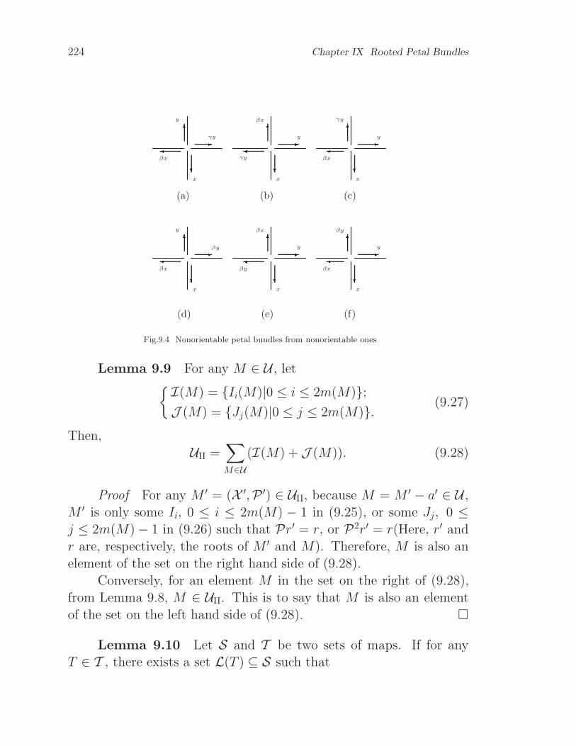
224 Chapter IX Rooted Petal Bundles
? 6 - ? 6 - ? 6 -x x x
βx βx
βxy
y yγy
γy
γy
(a) (b) (c)
? 6 - ? 6 - ? 6 -x x x
y
y yβy
βy
βy
βx βx
βx
(d) (e) (f)
Fig.9.4 Nonorientable petal bundles from nonorientable ones
Lemma 9.9 For any M ∈ U , let I(M) = Ii(M)|0 ≤ i ≤ 2m(M);J (M) = Jj(M)|0 ≤ j ≤ 2m(M). (9.27)
Then,
UII =∑
M∈U(I(M) + J (M)). (9.28)
Proof For any M ′ = (X ′,P ′) ∈ UII, because M = M ′ − a′ ∈ U ,
M ′ is only some Ii, 0 ≤ i ≤ 2m(M) − 1 in (9.25), or some Jj, 0 ≤j ≤ 2m(M)− 1 in (9.26) such that Pr′ = r, or P2r′ = r(Here, r′ and
r are, respectively, the roots of M ′ and M). Therefore, M is also an
element of the set on the right hand side of (9.28).
Conversely, for an element M in the set on the right of (9.28),
from Lemma 9.8, M ∈ UII. This is to say that M is also an element
of the set on the left hand side of (9.28).
Lemma 9.10 Let S and T be two sets of maps. If for any
T ∈ T , there exists a set L(T ) ⊆ S such that

IX.3 Nonorientable pedal bundles 225
(i) for any T ∈ T , |L(T )| = am(T ) + b and for S ∈ S, m(T ) =
m(S) − c, where a b and c are constants and m(T ) is an isomorphic
invariant, e.g., the size; and
(ii) S =∑
T∈TL(T ),
then
fS(x) = xc(bfT + axdfTdx
). (9.29)
Proof Because L(T ) provides a mapping from a map in T to a
subset of S and the cardinality of the subset is only dependent on the
parameter of the enumerating function(by (i)), and (ii) means that
the mapping provides a partition on S, then
x−cfS(x) =∑
T∈T(am(T ) + b)xm(T )
= b∑
T∈Txm(T ) + ax
∑
T∈Tm(T )xm(T )−1
= bfT + axdfTdx
.
This is (9.29) by multiplying xc to the two sides.
Theorem 9.3 The enumerating function g = fU(x) of nonori-
entable rooted petal bundles in the set U with size as the parameter
satisfies the equation as
4x2dg
dx= (1− 2x)g − x(h+ 2x
dh
dx);
dg
dx|x=0 = 1,
(9.30)
where h = fD(x) is the enumerating function of orientable rooted petal
bundles given by (9.9).
Proof Because (9.23) and (9.28) provides the mappings from
maps D ∈ D and U ∈ U to, respectively, a subset of UI with 2m(U)+1
elements and a subset of UII with 2(2m(U)+1) = 4m(U)+4 elements,

226 Chapter IX Rooted Petal Bundles
where D and U are 1 edge less than their images, from Lemma 9.10,
fUI(x) = x(h+ 2x
dh
dx) = xh+ 2x2dh
dx
and
fUII(x) = x(2g + 4x
dg
dx) = 2xg + 4x2dg
dx.
By (9.20) again,
g = xh+ 2x2dh
dx+ 2xg + 4x2dg
dx.
Via rearrangement, (9.30) is soon obtained.
IX.4 The number of pedal bundles
Because (9.9) provides the number of orientable rooted petal bun-
dles with size m, m ≥ 0, i.e.,
Hm =(2m− 1)!
2m−1(m− 1)!, (9.31)
for m ≥ 1. Of curse, H0 = 1.
Here, the number of nonorientable rooted petal bundles with size
m is evaluated only by the equation shown in (9.30). Let Gm be the
number of nonorientable rooted petal bundles with size m, m ≥ 1.
In fact, Gm, m ≥ 1, are determined by the recursion asGm = (4m− 2)Gm−1 +Hm, m ≥ 2;
G1 = 1.(9.32)
The solution of the recursion (9.32) is obtained, i.e.,
Gm =(2m− 1)!
2m−1(m− 1)!+
m∏
i=2
(4i− 2)
+
m−1∑
i=2
(2i− 1)!
2i−1(i− 1)!
m∏
j=i+1
(4j − 2).
(9.33)

IX.4 The number of pedal bundles 227
Example 9.5 When m = 1, there are one orientable rooted
petal bundle of 1 edge, i.e., M = (Kx, (x, γx)) and one nonorientable
rooted petal bundle of 1 edge, i.e., N = (Kx, (x, βx)) ∈ U .
By appending an edge Ky on M , 3 non-isomorphic nonorientable
rooted petal bundles of 2 edges are produced and shown in (a–c) of
Fig.9.3.
By appending an edge Ky on N , 6 non-isomorphic nonorientable
rooted petal bundles of 2 edges are produced and shown in (a–f) of
Fig.9.4. Then, G2 = 9 which is in agreement with that provided by
(9.32), or (9.33).
Now, Hm, Gm, and H(0)m for m ≤ 10 are listed in Table 9.1.
m Hm Gm H(0)m
1 1 1 12 3 9 23 15 105 54 105 1575 145 945 29295 426 10395 654885 1327 135135 17162145 4298 2027025 516891375 14309 34459425 17608766175 4862
10 654729075 669787843725 16796
Table 9.1 Numbers of rooted petal bundles in 10 edges
Lemma 9.11 For an integerm ≥ 1, the number of non-isomorphic
nonorientable rooted petal bundles with size m is
Gm = (2m − 1)Hm (9.34)
where Hm is given by (9.31).
Proof By induction. When m = 1, from H1 = 1, G1 = 1. (9.34)
is true.
Assume Gk satisfies (9.34) for any 1 ≤ k ≤ m− 1, m ≥ 2. Then,

228 Chapter IX Rooted Petal Bundles
from (9.32),
Gm = (4m− 2)Gm−1 +Hm
= (4m− 2)((2m−1 − 1)Hm−1) +Hm.
Since it can, from (9.31), be seen that
Hm = (2m− 1)Hm−1,
we have
Gm = (4m− 2)(2m−1 − 1)Hm
2m− 1+Hm
=
(4m− 2
2m− 1(2m−1 − 1) + 1
)Hm
= (2(2m−1 − 1) + 1)Hm
= (2m − 1)Hm.
This is (9.34).
Theorem 9.4 For an integer m ≥ 1, the number of non-
isomorphic rooted petal bundles with size m is
2m(2m− 1)!! (9.35)
where
(2m− 1)!! =m∏
i=1
(2i− 1). (9.36)
Proof Because of (9.34), the number of non-isomorphic petal
bundles with m edges is
Hm +Gm = 2mHm. (9.37)
By substituting (9.31) into (9.37), we have
2mHm = 2m × (2m− 1)!
2m−1(m− 1)!
= 2× (2m− 1)!
(m− 1)!
= 2m(2m− 1)!!.

IX.4 The number of pedal bundles 229
This is (9.35).
The theorem above reminds the number of embeddings of the
bouquet of size m
2m(2m− 1)!
derived from (1.10) as a special case. This is (m−1)! times the number
of rooted petal bundles with m edges.

Activities on Chapter IX
IX.5 Observations
A map with only one face is called a unisheet.
O9.1 Observe that there is a 1–to–1 correspondence between
the set of petal bundles and the set of unisheets.
O9.2 Think that what types of graphs can be as the under
graph of a unisheet and what type of graphs are not as the under
graph of a unisheet.
O9.3 Is any planar graph a under graph of a planar unisheet?
O9.4 Think about three ways to justify a map which is a planar
petal bundle.
O9.5 Discuss how to determine that a petal bundle is on the
projective plane.
O9.6 Discuss how to determine that a petal bundle is on the
torus.
O9.7 Discuss how to determine that a petal bundle is on the
Klein bottle.
O9.8 Discuss how to determine that a unisheet is on the plane.
O9.9 Discuss how to determine that a unisheet is on the pro-
jective plane.
O9.10 Discuss how to determine that a unisheet is on the torus.
O9.11 Discuss how to determine that a unisheet is on the Klein

IX.6 Exercises 231
bottle.
IX.6 Exercises
E9.1 Show that for any graph G, there exists a unisheet U such
that G is the under graph of U .
E9.2 Prove that the number of rooted unisheet with size m is
(2m− 1)!! =
m∏
i=1
(2i− 1).
E9.3 Prove that a unisheet is planar if, and only if, its under
graph is a tree.
E9.4 For an integer m ≥ 1, determine the number of rooted
petal bundles of size m on the torus.
E9.5 For an integer m ≥ 1, determine the number of rooted
petal bundles of size m on the projective plane.
A graph is said to be unicyclic if it has only one cycle.
E9.6 Prove that a unisheet is on the projective plane if, and
only if, its under graph is unicyclic.
A graph is said to be eves-cyclic if it has two fundamental circuits
incident.
E9.7 Prove that a unisheet is on the torus if, and only if, its
under graph is eves-cyclic.
E9.8 For an integer m ≥ 1, determine the number of non-
isomor- phic rooted petal bundles with size m on the projective plane.
E9.9 For an integer m ≥ 1, determine the number of non-
isomor- phic rooted petal bundles with size m on the torus.
E9.10 For an integer m ≥ 1, determine the number of non-
isomorphic rooted petal bundles with size m on the Klein bottle.

232 Activities on Chapter IX
E9.11 For an integer m ≥ 1, determine the number of non-
isomorphic rooted unisheets with size m on the projective plane.
E9.12 For an integer m ≥ 1, determine the number of non-
isomorphic rooted unisheets with size m on the Klein bottle.
A map of order 3 is also called tri-pole map.
E9.13 For a given integer m ≥ 1, determine the number of all
non-isomorphic rooted tri-pole maps with size m in the plane.
IX.7 Researches
R9.1 For two integers m ≥ 1 and p ≥ 2, determine the number
of rooted petal bundles with size m on the surface of orientable genus
p.
R9.2 For two integers m ≥ 1 and q ≥ 3, determine the number
of rooted petal bundles with size m on the surface of nonorientable
genus q.
R9.3 For two integers m ≥ 1 and p ≥ 2, determine the number
of rooted unisheets with size m on the surface of orientable genus p.
R9.4 For two integers m ≥ 1 and q ≥ 3, determine the number
of rooted unisheets with size m on the surface of nonorientable genus
q.
A map of order 2 is also called bi-pole map.
R9.5 For a given integer m ≥ 1, determine the number of all
non-isomorphic orientable rooted bi-pole maps with size m
R9.6 For a given integer m ≥ 1, determine the number of all
non-isomorphic nonorientable rooted bi-pole maps with size m
R9.7 For two integers m ≥ 1 and p ≥ 0, determine the number
of all non-isomorphic orientable rooted bi-pole maps with size m of

IX.7 Researches 233
the surface of genus p.
R9.8 For two integers m ≥ 1 and q ≥ 1, determine the number
of all non-isomorphic nonorientable rooted bi-pole maps with size m
on the surface of genus q.
R9.9 For a given integer m ≥ 1, determine the number of all
non-isomorphic orientable rooted tri-pole maps with size m
R9.10 For a given integer m ≥ 1, determine the number of all
non-isomorphic nonorientable rooted tri-pole maps with size m
R9.11 For two integers m ≥ 1 and p ≥ 1, determine the num-
ber of all non-isomorphic orientable rooted tri-pole maps with size m
of the surface of genus p.
R9.12 For two integers m ≥ 1 and q ≥ 1, determine the num-
ber of all non-isomorphic nonorientable rooted tri-pole maps with size
m on the surface of genus q.
R9.13 For two integers n ≥ 5 and p ≥ s(n) where
s(n) = ⌈(n− 3)(n− 4)
12⌉,
i.e., the least integer not less than the fractional (n− 3)(n− 4)/12(or
called the up-integer of the fractional), determine the number of rooted
maps whose under graph is the complete graph of order n with ori-
entable genus p.
R9.14 For two integers n ≥ 5 and p ≥ t(n) where
t(n) = ⌈(n− 3)(n− 4)
6⌉,
determine the number of rooted maps whose under graph is the com-
plete graph of order n with nonorientable genus q.
R9.15 For two integers n ≥ 3 and p ≥ c(n) where
c(n) = (n− 4)2n−3 + 1,
determine the number of rooted maps whose under graph is the n-cube
with orientable genus p.
234 Activities on Chapter IX
R9.16 For two integers n ≥ 3 and q ≥ d(n) where
d(n) = (n− 4)2n−2 + 2,
determine the number of rooted maps whose under graph is the n-cube
with nonorientable genus q.
R9.17 For three integers m,n ≥ 3 and p ≥ r(n) where
r(n) = ⌈(m− 2)(n− 2)
4⌉,
determine the number of rooted maps whose under graph is the com-
plete bipartite graph of order m+ n with orientable genus p.
R9.18 For three integers m,n ≥ 3 and q ≥ l(n) where
l(n) = ⌈(m− 2)(n− 2)
2⌉,
determine the number of rooted maps whose under graph is the com-
plete bipartite graph of order m+ n with nonorientable genus q.

Chapter X
Asymmetrized Maps
• From decomposing the set of rooted orientable maps, a quadratic
differential equation satisfied by the enumerating function with
size as the parameter is discovered and then a recursion formula is
extracted for determining the function.
• A quadratic equation of the enumerating function in company with
its partial values for rooted maps on the surface of orientable genus
0 is discovered with an extra parameter and then an explicit ex-
pression of the function with only size as a parameter is via char-
acteristic parameters extracted for each term summation free.
• From decomposing the set of rooted nonorientable maps, a nonlin-
ear differential equation satisfied by the enumerating function with
size as the parameter is discovered in company with the orientable
case and then a recursion formula is extracted for determining the
function.
• The numbers of orientable, nonorientable and total maps with
given size are, in all, obtained and then calculated for size not
greater than 10.
X.1 Orientable equation
It is from Corollary 8.7 shown that a map with symmetry be-

236 Chapter X Asymmetrized Maps
comes a map without symmetry whenever an element is chosen as the
root. Such a map with a root is called a rooted map.
Rooting is, in fact, a kind of simplification in mathematics, par-
ticularly in recognizing distinct combinatorial configurations for re-
ducing the complexity.
As soon as the rooted case is done, the general case can be re-
covered by considering the symmetry in a suitable way.
For maps, the estimation of the order of the automorphism group
of a map in the last chapter and the efficient algorithm for justifying
and recognizing if two maps are isomorphic in Chapter VII provide a
theoretical foundation for transforming rooted maps into non-rooted
maps. This will be seen in the next chapter.
The main purpose of this chapter is to present some methods for
investigating non-planar rooted maps as appendix to the monograph
Enumerative Theory of Maps[Liu7] in which most pages are for planar
maps, particularly rooted.
Let M be the set of all orientable rooted maps. For M =
(X ,P) ∈M, let
vx = (x)P = (x,Px, · · · ,P−1x) (10.1)
be the vertex incident with x ∈ X . The root is always denoted by r.
The rooted edge which is incident with r is denoted by a = Kr. The
rooting of M − a is taking Pδr as its root where
δ = mini|P ir 6∈ Kr, i ≥ 1. (10.2)
In fact,
δ =
1, if Pr 6= γr;
2, othewise.(10.3)
In virtue of Theorem 3.4, M − a is a map if, and only if, a is not
a harmonic loop except terminal link (or segmentation edge) of M .
Now, let us partition M into three parts: MI, MII and MIII,
i.e.,
M =MI +MII +MIII (10.4)

X.1 Orientable equation 237
whereMI = ϑ, i.e., consisted of the trivial map,MII andMIII are,
respectively, consisted of those with a as a segmentation edge and not.
Lemma 10.1 LetM〈II〉 = M − a|∀M ∈MII. Then,
M〈II〉 =M×M (10.5)
where × stands for the Cartesian product of two sets.
Proof For any M = (X ,P) ∈ M ×M, let M = M1 + M2,
Mi = (Xi,Pi), i = 1, 2. Assume M ′ = (X ′,P ′) such that X ′ = X+Kr′
and P ′ is different from P2 or P1 only at, respectively,
vr′ = (r′)P ′ = (r′, r2,P2r2, · · · ,P−12 r2)
or
vβr′ = (βr′)P ′ = (αβr′, r1,P1r1, · · · ,P−11 r1).
Since M ′ ∈ M and its rooted edge a′ = Kr′ is a segmentation
edge, M ′ ∈ MII. It is checked that M = M ′ − a′. Therefore, M ∈M〈II〉.
Conversely, for any M ∈ M〈II〉, we have M ′ ∈ MII such that
M = M ′ − a′ where a′ = Kr′. From M ′ ∈ MII, M = M1 +M2 where
M1,M2 ∈M. This implies that M ∈M×M.
It is seen from this lemma that there is a 1–to–1 correspondence
between M(∈M〈II〉, orM×M) and M ′(∈MII). Hence,
|MII| = |M×M|. (10.6)
For M = (X ,P) ∈MIII, because M −a is a map (Theorem 3.4),
from (10.3), the root r(M − a) of M − a has two possibilities: when
Pr(M) 6= γr(M), r(M − a) = Pr(M); otherwise,
r(M − a) = P2r(M).
Let M = (X , P) = M−a where X = X −Kr and P are different
from P only at
(r)P = (Pr,P2r, · · · ,P−1r),
(Pγr)P = (Pγr,P2γr, · · · ,P−1γr)
if a is not a loop;

238 Chapter X Asymmetrized Maps
otherwise, i.e., when a is a loop,
(r)P =
(P2r,P3r, · · · ,P−1r), γr = Pr;(Pr, · · · ,Ps−1r,Ps+1r, · · · ,P−1r),
if γr = Psr, s ≥ 2.
Since M(X ,P) is orientable, group Ψ = Ψγ,P has two orbits
rΨ and αrΨ on X . For M = (X , P) = M − a, group Ψ = Ψγ,Palso has two orbits
rΨ = rΨ − r, γrand
αrΨ = αrΨ − αr, βr.So, M is also orientable.
Furthermore, for every element y ∈ rΨ, is there exactly one
position of a = Kr, i.e., γr is in the angle 〈αy, P〉, for M ∈MIII such
that M = M − a. This means that inMIII, there are
|rΨ| =1
2|X | = 2m(M),
where m(M) is the size of M , non-isomorphic maps for producing M .
By considering for the case Pr = γr, in MIII, there are 2m(M) + 1
non-isomorphic maps for M altogether.
Example 10.1 Let
M = (Kx+Ky +Kz, (x, y, γz)(z, γx, γy))
where r = x is the root shown in Fig.10.1(a). Since it is orientable, the
orbit of group Ψ which r is in can be written as a cyclic permutation
as
(r)Ψ = (x, y, γz, z, γx, γy).
Then, Fig.10.1(b–h) presents all the 2m(M)+1 = 2 × 3+1 = 7 maps
in MIII, obtained by appending a = Kr on map M where (b) is for
Pr = γr and (c–h) are for those obtained by appending a = Kr in
the order of (r)Ψ from M .

X.1 Orientable equation 239K - U - Ur = x r = x
y y
γy γy
γxγx
zz
γzγz
Y+r
γr
(a) (b)
K - U - Ur = x r = x
y y
γy γy
γxγx
zz
γzγz
Æ Ur r
γr
γr
(c) (d)
K - U - Ur = x r = x
y y
γy γy
γxγx
zz
γzγz
i+ -r
r
γr
γr
(e) (f)

240 Chapter X Asymmetrized MapsK - U - Ur = x r = x
y y
γy γy
γxγx
zz
γzγz
Kr
γr
r
γr
(g) (h)
Fig.10.1 New maps obtained by appending an edge
Lemma 10.2 LetM〈III〉 = M − a|∀M ∈MIII. Then,
M〈III〉 =M. (10.7)
Proof Because for anyM ∈MIII, M−a is also a map (Theorem
3.4), thenM〈III〉 ⊆M.
Conversely, for any M ∈M, any one, e.g., M ′ of the 2m(M) +1
maps obtained by appending a′ from M in the above way is with
M ′ ∈MIII. Because M = M ′ − a′, then M ∈M〈III〉.
For convenience, let H(M) be the set of all the 2m(M) +1 maps
in MIII, obtained from M by appending an edge in the above way.
From Theorem 8.1, they are all mutually nonisomorphic in the sense
of rooting.
Lemma 10.3 ForMIII,
MIII =∑
M∈MH(M). (10.8)
Proof For any M = (X ,P) ∈ MIII, let M = (X , P) = M − a.Because a is not a segmentation edge, from Theorem 3.4 and Corollary
3.1, M ∈ M. By orientability, because r ∈ rΨ where Ψ = Ψγ,P,there exists y ∈ rΨ such that Py = γr, or Pr = γr. Because
|rΨ| = 2mM , the former has 2m(M) possibilities and the latter,
only one. This is the 2m(M) + 1 possibilities in H(M). Further,

X.1 Orientable equation 241
because M ∈M, M is an element of the set on the right hand side of
(10.8).
Conversely, for any M ∈ H(M), M ∈ M, Since M = M − a ∈M, by Theorem 3.4 and Corollary 3.1a is not a segmentation edge.
Therefore, M ∈MIII.
Furthermore, (10.8) provides a 1–to–1 correspondence between
the sets on its two sides. This enables us to construct all orientable
maps with the rooted edge not a segmentation edge from general ori-
entable maps with smaller size.
In order to determine the number of non-isomorphic orientable
rooted maps in M with size m ≥ 0, the enumerating function of set
MfM(x) =
∑
M∈Mxm(M) (10.9)
has to be investigated for a simpler form in infinite power series where
m(M) is the size of M . In the series form of (10.9), the coefficient
of the term with xm, m ≥ 0, is just the number of non-isomorphic
orientable rooted maps with size m.
From (10.4),
fM(x) = fMI(x) + fMII
(x) + fMIII(x). (10.10)
Lemmas above enable us to evaluate fMI(x), fMII
(x) and fMIII(x)
as functions of f = fM(x).
First, becauseMI contains only one map ϑ andm(ϑ) = 0, fMI(x)
contributes the constant term 1 of f , i.e.,
fMI(x) = 1. (10.11)
Lemma 10.4 ForMII,
fMII(x) = xf 2. (10.12)
Proof According to the 1–to–1 correspondence between MII
andM〈II〉 and that the former is with its size 1 greater than the latter

242 Chapter X Asymmetrized Maps
in the correspondence, by (10.6),
fMII(x) = x
∑
M∈M〈II〉
xm(M)
= x∑
M∈M×Mxm(M)
= x(∑
M∈Mxm(M))
2
= xf 2.
This is (10.12).
Lemma 10.5 ForMIII,
fMIII(x) = xf + 2x2df
dx. (10.13)
Proof From the 1–to–1 correspondence betweenMII andM〈II〉
and that the former is with its size 1 greater than the latter in the
correspondence, and then by Lemma 10.3 and Lemma 9.10,
fMIII(x) = x
∑
M∈M〈III〉
xm(M)
= x(f + 2xdf
dx)
= xf + 2x2df
dx.
This is (10.13).
Theorem 10.1 The differential equation about f
2x2df
dx= −1 + (1− x)f − xf 2;
f0 = f |x=0 = 1(10.14)
is well defined in the ring of infinite power series with all coefficients
nonnegative integers and the terms of negative powers finite. And,
the solution is f = fM(x).

X.2 Planar rooted maps 243
Proof Suppose f = F0 + F1x + F2x2 + · · · + Fmx
m + · · ·, Fi ∈Z+, i ≥ 0. Based on the first relation of (10.14), by equating the
coefficients on the two sits with the same power of x, the recursion
−1 + F0 = 0;
F1 − F0 − F 20 = 0;
Fm = (2m− 1)Fm−1 +m−1∑
i=0
FiFm−1−i,
m ≥ 2
(10.15)
is soon extracted. Then, F0 = 1(the initial condition), F1 = 2, · · ·, all
the coefficients of f can uniquely found from this recursion. Because
only addition and multiplication are used for evaluating all the coef-
ficients from the initial condition that F0 is an integer, Fm, m ≥ 1,
must all be integers. This is the first statement.
For the last statement, from (10.10) and (10.11–13), it is seen
that f = fM(x) satisfies the first relation of (10.14). And, f0 =
fM(0) = 1 is just the initial condition. By the uniqueness in the first
statement, the only possibility is f = fM(x).
Although the form of the equation in Theorem 10.1 is rather
simple, because of the occurrence of f 2, it is far from getting the
solution directly. In fact, it is an equation in the Riccati’s type. It has
no analytic solution in general.
X.2 Planar rooted maps
Let T be the set of all planar rooted maps. Because it looks hard
to decompose T into some classes so that each class can be produced
by T with only size as the parameter. Now, another parameter for
a map M , i.e., the valency of the rooted vertex n(M), is introduced.
The enumerating function of T is
t(x, y) = fT (x, y) =∑
M∈Txm(M)yn(M) (10.16)

244 Chapter X Asymmetrized Maps
where m(M) is still the size of M .
Assume that T is partitioned into three classes: T0, T1 and T2,
i.e.,
T = T0 + T1 + T2 (10.17)
where T0 = ϑ, T1 and T1 are the sets of planar rooted maps with
the rooted edge, respective a loop and a link(not loop).
For M ∈ T , let a = Kr be the rooted edge of M with the root
r = r(M). For maps Mi ∈ T (i=1 and 2), let ai = Kri be the rooted
edge of Mi with the root ri = r(Mi).
The 1-addition of two maps M1 = (X1,P1) and M2 = (X2,P2)
is to produce the map M1 + · M2 = M1 ∪M2 with the root r = r1provided M1 ∩M2 = vr where vr = (〈r1〉P1
, 〈r2〉P2).
Lemma 10.6 Let T〈1〉 = M − a|∀M ∈ T1, then
T〈1〉 = T ×· T (10.18)
where T ×· T = M1 +M2|∀M1,M2 ∈ T is called the 1-product of Twith itself.
Proof For any M = (X ,P) ∈ T〈1〉, let M ′ = (X ′,P ′) ∈ T1 such
that M ′ − a′ = M . Because a′ = Kr′ is a loop,
(r′)P ′ = (r′,P ′r′, · · · , γr′, · · · ,P ′−1r′).
From the planarity, M ′−a′ = M1+·M2, Mi = (Xi,Pi), i = 1, 2, where
X = X1 +X2 = X ′−Kr′, P1 and P2 are different from P only at (r)Pbecoming, respectively,
(r1)P1= (P ′r′,P(P ′r′), · · · ,P ′−1
γr′)
where γ = αβ and
(r2)P2= (P ′γr′,P(P ′γr′), · · · ,P ′−1
r′).
This implies M ∈ T ×· T .
Conversely, for M ∈ T ×· T , because M = M1 + M2, let M ′ =M + a′, a′ = Kr′, such that
(r′)P ′ = (r′, 〈r1〉P1, γr′, 〈r2〉P2
),
X.2 Planar rooted maps 245
then M ′ ∈ T and M = M ′− a′. Since a′ is a loop, M ′ ∈ T1 and hence
M ∈ T〈1〉.
Because this lemma presents a 1–to–1 correspondenceM = M1+
M2 between M ∈ T〈1〉 and M1,M2 ∈ T with m(M) = m(M1)+m(M2)
and n(M) = n(M1) + n(M2), the enumerating function of T〈1〉
fT〈1〉(x, y) =∑
M∈T ×· Txm(M)yn(M)
=∑
M1,M2∈Txm(M1)+m(M2)yn(M1)+n(M2)
= (∑
M∈Txm(M)yn(M))
2
= t2(x, y).
(10.19)
Then, from the 1–to–1 correspondence between T1 and T〈1〉 with
the former of size 1 greater than the latter and the former of the rooted
vertex valency 2 greater than the latter, the enumerating function of
T1 is
fT1(x, y) = xy2fT〈1〉(x, y) = xy2t2(x, y). (10.20)
However, for T2, the correspondence between T2 and T〈2〉 = M •a|∀M ∈ T2 with the former of size 1 greater than the latter is not of
1–to–1 where M • a is the contraction of the rooted edge a on map
M . The root on M • a is defined to be Pγr when Pγr 6= γr; or
(Pγ)2r otherwise. Because a is a link, this is a basic transformation.
According to Chapter V, M − a is planar if, and only if M is. Hence,
T〈2〉 = T . (10.21)
Further, observe what a correspondence between T2 and T is.
For M = (X ,P) ∈ T , let (r)P = (r,Pr, · · · ,Pn(M)−1r) where
n(M) is the valency of the rooted vertex vr on M . By splitting a link
at vr, all those obtained are still planar because this operation is a
basic transformation. For doing this, there are n(M) + 1 possibilities
altogether.

246 Chapter X Asymmetrized Maps
Let Mi = (Xi,Pi), 0 ≤ i ≤ n(M) be all the n(M) + 1 maps
obtained from M by splitting an edge at the rooted vertex vr = (r)Pas
vri=
(r0, 〈r〉P), while vβr0= (γr0);
(r1,Pr, · · · ,Pn(M)−1r),while vβr1= (γr1, r);
(r2,P2r, · · · ,Pn(M)−1r),while vβr2= (γr2, r,Pr);
· · · · · ·(rn(M)−1,Pn(M)−1r),
while vβrn(M)−1= (γrn(M)−1, r, · · · ,Pn(M)−2r);
(rn(M)),while vβrn(M)= (γrn(M), 〈r〉P).
(10.22)
Lemma 10.7 For a map M ∈ T , let
K(M) = Mi|i = 0, 1, 2, · · · , n(M)
where Mi, 0 ≤ i ≤ n(M), are given by (10.22). Then,
T2 =∑
M∈TK(M). (10.23)
Proof For any M ∈ T2, because a = Kr is a link, from (10.21),
M • a ∈ T and from (10.22), M ∈ K(M • a). Therefore M is an
element of the set on the right hand side of (10.23).
Conversely, for M is an element of the set on the right of (10.23),
there exists a map M ′ ∈ T such that M ∈ K(M ′). Because all maps
in K(M) are planar if, and only if, M ′ is planar, M ∈ T as well.
Moreover, from (10.22), the rooted edge a is a link, M ∈ T2. This
meas that M an element of the set on the left hand side of (10.23).
Because (10.23) presents a 1–to–1 correspondence between maps
with the same size on its two sides and the valency of rooted vertex
of Mi(0 ≤ i ≤ n(M)) is n(M) − i for any M ∈ T , the enumerating

X.2 Planar rooted maps 247
function of T2 is
fT2(x, y) =∑
M∈T2xm(M)yn(M)
= xy∑
M∈T(
n(M)∑
i=0
yi)xm(M)
= xy∑
M∈T
1− yn(M)+1
1− y xm(M)
=xy
1− y (t0 − yt)
(10.24)
where t = t(x, y) and t0 = t(x, 1).
Theorem 10.2 The enumerating function t = t(x, y) of planar
rooted maps satisfies the equation as
xy2(1− y)t2 − (1− y + xy2)t+ xyt0 + (1− y) = 0 (10.25)
where t0 = t(x, 1).
Proof From (10.17),
t = fT0(x, y) + fT1(x, y) + fT2(x, y).
Because T0 = ϑ and ϑ has no edge, fT0(x, y) = 1. From (10.20) an
(10.24),
t = 1 + xy2t2 +xy
1− y (t0 − yt).
Via rearrangement of terms, (10.25) is soon found.
Although (10.25) is a quadratic equation, because the occurrence
of t0 which is also unknown and the equation becomes an identity when
y = 1, complication occurs in solving the equation directly.
The discriminant of the equation (10.25), denoted by D(x, y), is
D(x, y) = (xy2 − y + 1)2 − 4(y − 1)xy2(y − 1− xyt0)
= 1− 2y + (1− 2x)y2 + (x2 + 2x

248 Chapter X Asymmetrized Maps
−H(x))y3 +H(x)y4 (10.26)
where
H(x) = 4x2t0 + x2 − 4x. (10.27)
Assume that D(x, y) has the form as
D(x, y) = (1− θy)2(1 + ay + by2)
= 1− (2θ − a)y + (θ2 − 2aθ + b)y2
+θ(aθ − 2b)y3 + θ2by4. (10.28)
By comparing with (10.26),
θ = 1 +a
2, (10.29)
and
1− 2x = θ(4− 3θ) + b;
x2 + 2x−H(x) = θ(2(θ − 1)θ − 2b);
H(x) = θ2b.
(10.30)
Then, an equation about b with θ as the parameter is found as
1
4(1− 4θ + 3θ2 − b)2
+ 1− 4θ + 3θ2 − b− θ2b
= 2(θ − 1)θ2 − 2θb.
By rearrangement, it becomes
b2 − (10θ2 − 16θ + 6)b+ (9θ4 − 32θ3
+42θ2 − 24θ + 5) = 0. (10.31)
The discriminant of (10.31) is
(10θ2 − 16θ + 6)2 − 4(9θ4 − 32θ3 + 42θ2 − 24θ + 5)
= 64θ4 − 192θ3 + 208θ2 − 96θ + 16
= (8θ2 − 12θ + 4)2.
Therefore,
b = (θ − 1)2, or 9θ2 − 14θ + 5 = (9θ − 5)(θ − 1).

X.2 Planar rooted maps 249
The latter has to be chosen in our case. By the last relation of
(10.30),
H(x) = θ2(9θ − 5)(θ − 1).
From the first relation of (10.30) and (10.27), the expressions for
x and b0 with parameter θ are extracted as
x = (3θ − 2)(1− θ);b0 =
4θ − 3
(3θ − 2)2.
(10.32)
This enables us to get b0 as a power series of x as
b0(x) =∑
m≥0
2× 3m(2m)!
m!(m+ 2)!xm. (10.33)
by eliminating the parameter θ via Lagrangian inversion. More about
this method can be seen in the monograph[Liu8].
Example 10.2 For m = 2, it is known from (10.33) that the
number of non-isomorphic planar rooted maps is the coefficient of x2.
That is 9.
Because there are 4 non-isomorphic planar maps of size 2 as
shown in Fig.10.2. The arrows on the same map represent the roots
of non-isomorphic rooted ones. Such as there are, respectively, 2, 2, 1
and 4 non-isomorphic rooted maps in (a), (b), (c) and (d) of Fig.10.2
to get 9 altogether.
U 6? K K M?6(a) (b) (c) (d)
Fig.10.2 Planar rooted maps of two edges

250 Chapter X Asymmetrized Maps
X.3 Nonorientable equation
Let Nm be the set of nonorientable rooted maps of size m. Of
course, m ≥ 1. And, let Nm be partitioned into N (I)m and N (II)
m , i.e.,
Nm = N (I)m +N (II)
m (10.34)
where N (I)m = N |N ∈ Nm, N − a orientable and
N (II)m = Nm −N (I)
m = N |N ∈ Nm, N − a nonorientable,a = er(N) is still the rooted edge.
Lemma 10.8 Let N 〈I〉m = N − a|∀N ∈ N (I)m , then
N 〈I〉m =Mm−1 (10.35)
whereMm−1 is the set of orientable rooted maps of size m−1, m ≥ 1.
Proof Because of the nonorientability of N ∈ N (I)m and the ori-
entability of N − a, from Corollary 3.1, a is not a segmentation edge.
Based on Theorem 3.4, N − a is always an orientable map. So, for
any N ∈ N 〈I〉m , N ∈Mm−1, m ≥ 1. This implies N 〈I〉m ⊆Mm−1.
Conversely, for any N = (X ,P) ∈Mm−1, by appending an edge
a′ on N , N ′ = (X ′,P ′) is obtained where X ′ = X + Kr′ and P ′ is
different from P only at the vertex
(r′)P ′ = (r′, βr′, 〈r〉P).Since Kr′ is not a segmentation edge, from Theorem 3.7, N ′ is a
map. And since βr′ ∈ r′Ψ′,Ψ′ = ΨP ′,γ, from Theorem 4.1, N ′
is nonorientable. Further, because N = N ′ − a′ is orientable and
m(N) + 1 = m(N ′) = m, N ∈ N 〈I〉m . This impliesMm−1 ⊆ N 〈I〉m .
For any M = (X ,P) ∈Mm, since M is orientable, assume
rΨ = r, ψ1r, · · · , ψ2m−1r,ψi ∈ Ψ = Ψγ,P, i = 1, 2, · · · , 2m(M) − 1 = 2m − 1. By appending
the edge r′,
A(M) = A0(M), A1(M), · · · , A2m(M)

X.3 Nonorientable equation 251
is obtained where Ai(M) = M+eri= (Xi,Pi) such that Xi = X +Kri
and Pi is determined in the following manner:
βr0 in the angle 〈αP−1r, r〉βri(i = 1, 2, · · · , 2m(M)− 1) in the angle 〈αP−1ψir, ψir〉,βr2m(M) in the angle 〈r, αP−1r〉.
Because βri ∈ riΨiwhere Ψi = Ψγ,Pi, i = 0, 1, · · · , 2m(M),
from Theorem 4.1, Ai are all nonorientable. Because Ai(M) − eri∈
Mm, Ai(M) ∈ N (I)m+1, 0 ≤ i ≤ 2m(M). From Lemma 10.8,
N (I)m+1 =
∑
M∈Mm
A(M) (10.36)
m ≥ 0. Of course,M0 consists of only the trivial map.
For N (II)m , two cases should be considered: N (N)
m and N (T)m , i.e.,
N (II)m = N (N)
m +N (T)m (10.37)
whereN (N)
m = N |∀N ∈ N (II)m , a = er is a terminal,
or segmentation edgeand
N (T)m = N |∀N ∈ N (II)
m , a is neither terminal
nor segmentation edge.Of course, N (T)
m = N (II)m −N (N)
m .
Lemma 10.9 Let N 〈N〉m = N − a|∀N ∈ N (N)m . Then,
N 〈N〉m =∑
n1+n2=m−1n1,n2≥0
Mn1×Nn2
+∑
n1+n2=m−1n1,n2≥0
Nn1×Mn2
+∑
n1+n2=m−1n1,n2≥0
Nn1×Nn2
(10.38)
where × represents the Cartesian product of sets.
Proof Easy to see except for noticing that N−a has a transitive
block which is the trivial map when a is a terminal edge.

252 Chapter X Asymmetrized Maps
Lemma 10.10 Let N 〈T〉m = N − a|∀N ∈ N (T)m . Then,
N 〈T〉m = Nm−1 (10.39)
where m ≥ 2.
Proof Because a = er is neither terminal nor segmentation edge,
from Theorem 3.4, N ∈ N 〈T〉m . By the nonorientability and the size
m− 1, N ∈ Nm−1, i.e.,
N 〈T〉m ⊆ Nm−1.
On the other hand, for any N = (X ,P) ∈ Nm−1, we have N ′ =(X ′,P ′) such that X ′ = X + Kr′ and P ′ is different from P only
at the vertex (r′)P ′ = (r′, γr′, 〈r〉P). Since N is nonorientable and
a′ = Kr′ is neither terminal nor segmentation edge, N ′ ∈ N (T)m . Thus,
N = N ′ − a′ ∈ N 〈T〉m . This implies
Nm−1 ⊆ N 〈T〉m .
In consequence, the lemma is proved.
One attention should be paid to is that whenm = 1, there is only
one nonorientable map (Kr, (r, βr)), and (Kr, (r, βr)) ∈ N (I). Thus,
(10.39) is meaningful only for m ≥ 2.
On the basis of this lemma, it is necessary to see how many
N ′ ∈ N (T)m+1 can be produced from one N ∈ Nm such that N = N ′−a′.
Because N is nonorientable, let I = r, ψ1r, ψ2r, · · · , ψ2m−1r be
consists of half the elements in rΨ = X , Ψ = Ψγ,P, such that for
any x ∈ I, Kx ∩ I = x, γx. Two cases are now considered.
Case 1 For any N = (X ,P) ∈ Nm, let
B(N) = B0(N), B1(N), B2(N), · · · , B2m(N)
where Bj(N) = (Xj,Pj) = N + erj, j = 0, 1, 2, · · · , 2m, have
βr0 in the angle 〈αP−1r, r〉,βrj(j = 1, 2, · · · , 2m− 1) in the angle 〈αP−1ψjr, jr〉,βr2m in the angle 〈r, αP−1r〉.

X.3 Nonorientable equation 253
Case 2 For any N = (X ,P) ∈ Nm, let
C(N) = C0(N), C1(N), C2(N), · · · , C2m(N)
where Cj(N) = (Yj,Qj) = N + erj, j = 0, 1, 2, · · · , 2m, have
γr0 in the angle 〈αP−1r, r〉,γrj(j = 1, 2, · · · , 2m− 1) in the angle 〈αP−1ψjr, jr〉,γr2m in the angle 〈r, αP−1r〉.
On the basis of Lemma 10.10, from the conjugate axiom,
N (T)m+1 =
∑
N∈Nm
(B(N) + C(N)) (10.40)
for m ≥ 1.
Because N = N1 +N2 + · · ·, the enumerating function
fN (x) =∑
m≥1
(∑
N∈Nm
1)xm = fN (I)(x) + fN (II)(x)
= fN (I)(x) + fN (N)(x) + fN (T)(x).
(10.41)
Lemma 10.11 For N (I) = N (I)1 +N (I)
2 + · · ·,
fN (I)(x) = xfM + 2x2dfMdx
(10.42)
where fM = fM(x) is the enumerating function of orientable rooted
maps determined by equation (10.14).
Proof On the basis of (10.35–36), from Lemma 9.10, the lemma
is obtained .
Lemma 10.12 For N (N) = N (N)1 +N (N)
2 + · · ·,
fN (N)(x) = 2xfMfN + xf 2N (10.43)
where fM = fM(x) as in (10.10) and fN = fN (x) as in (10.41).
Proof A direct result of Lemma 10.9.

254 Chapter X Asymmetrized Maps
Lemma 10.13 For N (T) = N (T)1 +N (T)
2 + · · ·,
fN (T)(x) = 2xfN + 4x2dfNdx
. (10.44)
Proof On the basis of Lemma 10.10 with its extension (10.40),
from Lemma 10.11, (10.44) is soon obtained.
Theorem 10.3 The following equation aboutf
4x2df
dx= a(x)f − xf 2 − 2xb(x);
df
dx
∣∣∣x=0
= 1
(10.45)
where a(x) = 1− 2x− 2xfM;
b(x) = fM − 2xdfMdx
is well defined in the ring of power series with all coefficients non-
negative integers and negative powers finite. And, the solution is
f = fN (x).
Proof Let f = N1x +N2x2 +N3x
3 + · · ·, then from (10.45) all
the coefficients can be determined by the recursion
Nm = (4m− 2)Nm−1 + (2m− 1)Fm−1
+2
m−1∑
i=1
NiFm−1−i +
m−2∑
i=1
NiNm−1−i,
m ≥ 2;
N1 = 1,
(10.46)
where Fm, m ≥ 0, are known in (10.15). Because all Nm, m ≥ 1,
determined by (10.46) are positive integers, the former statement is
true. The latter is directly deduced from (10.41–44).

X.4 Gross equation 255
X.4 Gross equation
LetRm be the set of general(orientable and nonorientable) rooted
maps with size m, m ≥ 0. Of course, R0 consists of only the trivial
map.
For m ≥ 1, Rm is partitioned into two subsets R(N)m and R(T)
m ,
i.e.,
Rm = R(N)m +R(T)
m (10.47)
whereR(N)
m = R|∀R ∈ Rm, er(R) is a terminal link
or segmentation edgeand
R(T)m = R|∀R ∈ Rm, er(R) is neither terminal
nor segmentation edge.
Of course, R(T)m = Rm −R(N)
m .
Lemma 10.14 Let R〈N〉m = R − a|∀R ∈ R(N)m , then
R〈N〉m =∑
n1+n2=m−1n1,n2≥0
Rn1×Rn1
, (10.48)
m ≥ 1.
Proof For any R ∈ R(N)M , because a = er(R) is a terminal link
or a segmentation edge, R − a has two transitive block (when a is a
terminal link, the trivial map is seen as a transitive block in its own
right), R− a = R1 +R2 and R1 ∈ Rn1, R2 ∈ Rn2
. In other words, the
set on the left hand side of (10.48) is a subset of the set of its right.
Conversely, for any R1 = (X1,P1) ∈ Rn1and R2 = (X2,P2) ∈
Rn2, by appending a = er, R = (X ,P) is obtained where X = X1 +
X2 +Kr and P is different from P1 and P2 only at the vertices (r)P =
(r, 〈r1〉P1) and (γr)P = (γr, 〈r2〉P2
). It is easily checked that R ∈ Rm,
m = n1 + n2 + 1. In other words, the set on the right hand side of
(10.48) is a subset of the set on the left.
256 Chapter X Asymmetrized Maps
Since R = R0 +R1 +R2 + · · ·, the enumerating function
fR(x) =∑
m≥0
(∑
R∈Rm
1)xm
= fR0(x) + fR(N)(x) + fR(T)(x),
(10.49)
where R(N) = R(N)1 +R(N)
2 + · · · and R(T) = R(T)1 +R(T)
2 + · · ·.First, because R0 consists of only the trivial map,
fR0(x) = 1. (10.50)
Then, from Lemma 10.14,
fR(N)(x) = xf 2R, (10.51)
where fR = fR(x).
In order to evaluate fR(T)(x), R(T) has to be decomposed.
Lemma 10.15 Let R〈T〉m = R − a|∀R ∈ R(T)m , then
R〈T〉m = Rm−1, (10.52)
where m ≥ 1.
Proof For any R′ ∈ R(T)m , because a′ = er′ is neither terminal
link nor segmentation edge, from Theorem 3.4, R = R′ − a′ ∈ Rm−1.
This implies
R〈T〉m ⊆ Rm−1.
Conversely, for any R = (X ,P) ∈ Rm−1, by appending the edge
a′ = Kr′, R′ = (X ′,P ′) is obtained where X ′ = X +Kr′ and P ′ is dif-
ferent from P only at the vertex (r′)P ′ = (r′, γr′, 〈r〉P). From Theorem
3.7, R′ ∈ Rm. Because a′ is neither terminal link nor segmentation
edge and R = R′ − a′, R ∈ R〈T〉m . This implies
Rm−1 ⊆ R〈T〉m .
The lemma is proved.
Based on this, what should be further considered for is how many
R′ ∈ R(T)m+1 can be produced from one R ∈ Rm such that R = R′− a′.

X.4 Gross equation 257
Because R is a map(orientable, or nonorientable), let
I = r, ψ1r, ψ2r, · · · , ψ2m−1r
be the set of elements in correspondence with a primal trail code, or
dual trail code. For any x ∈ I, Kx∩ I = x, γx has two possibilities
as cases.
Case 1 For any R = (X ,P) ∈ Rm, let
D(R) = D0(R), D1(R), D2(R), · · · , D2m(R)
where Dj(R) = (Xj,Pj) = R+ erj , j = 0, 1, 2, · · · , 2m, have
βr0 in the angle 〈αP−1r, r〉,βrj(j = 1, 2, · · · , 2m− 1) in the angle 〈αP−1ψjr, jr〉,βr2m in the angle 〈r, αP−1r〉.
Cases 2 For any R = (X ,P) ∈ Rm, let
E(R) = E0(R), E1(R), E2(R), · · · , E2m(R)
where Ej(R) = (Yj,Qj) = R + erj, j = 0, 1, 2, · · · , 2m, have
γr0 in the angle 〈αP−1r, r〉,γrj(j = 1, 2, · · · , 2m− 1) in the angle 〈αP−1ψjr, jr〉,γr2m in the angle 〈r, αP−1r〉.
Based on Lemma 10.15, from the conjugate axiom,
R(T)m+1 =
∑
R∈Rm
(D(R) +E(R)) (10.53)
for m ≥ 1.
Because R(T) = R(T)1 + R(T)
2 + · · ·, from Lemma 10.15 with its
extension (10.53) and Lemma 9.10, the enumerating function
fR(T)(x) = 2xfR + 4x2dfRdx
(10.54)

258 Chapter X Asymmetrized Maps
Theorem 10.4 The equation about f
4x2df
dx= −1 + (1− 2x)f − xf 2;
f0 = f(0) = 1(10.55)
is well defined in the ring of power series with coefficients all nonneg-
ative integers and terms of negative power finite. And, the solution is
f = fR(x).
Proof In virtue of the initial condition of equation (10.55), as-
sume f = R0 + R1x + R2x2 + · · ·. Of course, R0 = f0 = 1. Further,
from equation (10.55), the recursion
Rm = (4m− 2)Rm−1 +
m−1∑
i=0
RiRm−1−i,
m ≥ 1;
R0 = 1
(10.56)
is soon found for determine all the coefficients Rm, m ≥ 0. It is easily
checked that all of them are positive integers and hence the former
statement is true.
The latter is a direct result of (10.50–51) and (10.53).
X.5 The number of rooted maps
First, let σm = (F0, F1, · · · , Fm), m ≥ 0, be the m+1 dimensional
vector where Fm, m ≥ 0, are the number of non-isomorphic orientable
rooted maps with size m. And, σRM = (Fm, Fm−1, · · · , F0) called the
reversed vector of the vector σm. Easy to check that
σTRm = ((σm)T)R = ((σm)R)T = σRT
m (10.57)
where T the transposition of a matrix.
The recursion (10.15) for determining Fm, m ≥ 0, becomes
Fm = (2m− 1)Fm−1 + σm−1σTRm−1,
m ≥ 1;
F0 = 1.
(10.58)

X.5 The number of rooted maps 259
By (10.58), the number of non-isomorphic orientable rooted maps
with size m, m ≥ 1, can be calculated. In the first column of Table
10.1, Fm, m ≤ 10, are listed.
Then, let δm = (N1, N2, · · · , N1) where Nm is the number of non-
isomorphic nonorientable rooted maps with size m for m ≥ 1.
The recursion (10.46) for determining Nm, m ≥ 1, becomes
Nm = (4m− 2)Nm−1 + (2m− 1)Fm−1
+2δm−1σTRm−2 + δm−2δ
TRm−2,
m ≥ 2;
N1 = 1
(10.59)
where σm−2 is given in (10.58).
By (10.59), the number Nm can be calculated for m ≥ 1. In the
second column of Table 10.1, Nm, m ≤ 10, are listed.
Finally, let ρm = (R0, R1, · · · , Rm) where Rm is the number of
non-isomorphic general maps with size m for m ≥ 0.
The recursion (10.56) becomes
Rm = (4m− 2)Rm−1 + ρm−1ρTRm−1,
m ≥ 1;
R0 = 1.
(10.60)
By (10.60), the number Rm can be calculated for m ≥ 0. In the
third column of Table 10.1, Rm, m ≤ 10, are listed.
From those numbers in Table 10.1, it is also checked that the
enumerating functions fM(x), fN (x) and fR(x) of, respectively, non-
isomorphic orientable, nonorientable and general(orientable and nonori-
entable) rooted maps with size as the parameter satisfy the relation
as
fR(x) = fM(x) + fN (x). (10.61)

260 Chapter X Asymmetrized Maps
m Fm Nm Rm
0 1 0 11 2 1 32 10 14 243 74 223 2974 706 4190 48965 8162 92116 1002786 110410 2339894 24503047 1708394 67825003 695333978 29752066 2217740030 22474920969 576037442 80952028936 81528066378
10 12277827850 3268104785654 3280382613504
Table 10.1 Numbers of rooted maps with size less than 11
Activities on Chapter X
X.6 Observations
O10.1 Because a surface can be seen as a polygon with even
edges pairwise identified in the plane, think that whether, or not, a
map on a surface rather than plane can always represented by a planar
one. If it can, explain the reason, or provide an example otherwise.
O10.2 For a rooted map M , let m(M) and l(M) be, respec-
tively, the size and the valency of root-face in M , observe the numbers
of non-isomorphic planar rooted maps for m(M), l(M) ≤ 3.
Similarly, do the same with the valency of root-vertex s(M) in-
stead of l(M).
A map with all its faces of 3-valent except for the root-face is
called a near triangulation.
O10.3 For a near triangulation T , letm(T ) and l(T ) be, respec-
tively, the size and the root-face valency of T . Observe the numbers
of non-isomorphic planar rooted near triangulations for m, l ≤ 4.
Similarly, do the same with the valency of root-vertex s instead
of l.
A map with all its faces of valency 4 except for the root-face is
called a near quadrangulation.
O10.4 For a near triangulation Q, let m(Q) and l(Q) be,
respectively, the size and the root-face valency of TQ. Observe the
numbers of non-isomorphic planar rooted near quadrangulation for m,
l ≤ 5.

262 Activities on Chapter X
Similarly, do the same with the valency of root-vertex s instead
of l.
A planar map from which the result of deleting all the edges on
a face is a tree is called a Halin map. The face is said to be specific.
O10.5 Evaluate the number of non-isomorphic rooted Halin
maps with the root on the specific face by the parameters: the size m
and the valency l of the specific face for m ≥ 6 and l ≥ 3.
O10.6 Try, by edge contraction, to determine the enumerating
function of general rooted maps with the size as the parameter.
O10.7 Try, by edge contraction, to determine the enumerating
function of rooted petal bundles with the size an the root-face valency
as the two parameters.
O10.8 Try, by directly solving the equation (9.7), to determine
the enumerating function of orientable rooted petal bundles h.
O10.9 Try, by directly solving the equation (9.30), to deter-
mine the enumerating function of nonorientable rooted petal bundles
g.
O10.10 Observe the numbers of general Eulerian rooted maps
with the size smaller.
X.7 Exercises
For a map, if the result of deleting all inner vertices(not articulate
vertex, i.e., a vertex of valency 1, or a terminal) of a spanning tree is,
itself, a travel with only one vertex of valency probably greater than
2, then it is called a pan-Halin map. Because this travel is still a map
and becomes a petal bundle via decreasing subdivision, such a petal
bundle is called the base map of the pan-Halin map.
A pan-Halin map of which the base map is of size 2p and ori-
entable genus p ≥ 0, or of size q and nonorientable genus q ≥ 1, is
said to be pre-standard . If a pre-standard pan-Halin map has its base

X.7 Exercises 263
map with each edge incident with at least one terminal of the tree,
then it is said to be standard.
Let HpsH be the set of all pre-standard pan-Halin rooted maps.
The root rH for H ∈ HpsH is chosen be an element incident with the
vertex and the face of the base map of H.
For any H = (X ,P) ∈ HpsH, the tree T on H is seen as a
planted tree(a plane tree with the root-vertex of valency 1) with its
root rT = P(Pγ)trH where
t = mins|(Pγ)srH incident with a terminal of T.
E10.1 Given the partition of vertices according to their va-
lencies on a planted tree j = (j1, j2, · · · , ), i.e., ji, i ≥ 1, is the
number of unrooted vertices of valency i, prove that the number of
non-isomorphic planted trees with the partition is
(n− 1)!
j!
where
n = 1 +∑
i≥1
ji,
i.e., the order, and j! =∏
i≥1 ji!.
E10.2 Given the vertex partition s = (s2, s3, · · ·), prove that
the number of non-isomorphic pre-standard pan-Halin rooted maps
with the partition and their base maps of size m on a surface of ori-
entable genus p is
2m
(m+ 2p− 1
2p− 1
)(s3
m
)n!m
s!
where
n+ 2 =∑
i≥2
si, and s! =∏
s≥2
si!.
E10.3 Given the vertex partition s = (s2, s3, · · ·), Prove that
the number of non-isomorphic pre-standard pan-Halin rooted maps
264 Activities on Chapter X
with the partition and their base maps of sizem on a surface of nonori-
entable genus q is
2m
(m+ q − 1
q − 1
)(s3
m
)n!m
s!
where
n+ 2 =∑
i≥2
si, and s! =∏
s≥2
si!.
E10.4 Given the vertex partition s = (s2, s3, · · ·), prove that
the number of non-isomorphic standard pan-Halin rooted maps with
the partition and their base maps of size m on a surface of orientable
genus p is
2m
(m− 1
2p− 1
)(s3
m
)n!m
s!
where
n+ 2 =∑
i≥2
si,
and s ≥ 0, s 6= 0, m ≥ 2p ≥ 1.
E10.5 Given the vertex partition s = (s2, s3, · · ·), prove that
the number of non-isomorphic standard pan-Halin rooted maps with
the partition and their base maps of size m on a surface of nonori-
entable genus q is
2m
(m− 1
q − 1
)(s3
m
)n!m
s!
where
n+ 2 =∑
i≥2
si,
and s ≥ 0, s 6= 0, m ≥ q ≥ 1.
E10.6 Evaluate the number of near triangulations of size m on
the projective plane.
E10.7 Evaluate the number of near triangulations of size m on
the Klein bottle.

X.8 Researches 265
E10.8 Evaluate the number of rooted quadrangulations of size
m on the projective plane.
E10.9 Evaluate the number of near quadrangulations of size m
on the Klein bottle.
E10.10 Determine the enumerating function of rooted petal
bundles with the size as the parameter on the torus.
E10.11 Determine the enumerating function of rooted petal
bundles with the size as the parameter on the projective plane.
E10.12 Determine the enumerating function of orientable two
vertex rooted maps with size as the parameter.
E10.13 Determine the enumerating function of nonorientable
two vertex rooted maps with size as the parameter.
E10.14 Establish an equation satisfied by the enumerating func-
tion of general non-separable rooted maps.
E10.15 Establish an equation satisfied by the enumerating func-
tion of general Eulerian rooted maps.
A map is said to be loopless if its under graph has no self-loop.
E10.16 Establish an equation satisfied by the enumerating func-
tion of general loopless rooted maps.
A map is said to be simple if its under graph has neither self-loop
nor multi-edge.
E10.17 Establish an equation satisfied by the enumerating func-
tion of general simple rooted maps.
X.8 Researches
R10.1 Given a relative genus g 6= 0(the case g = 0 is solved),
determine the number of rooted near triangulations of size m ≥ |g| on

266 Activities on Chapter X
a surface of genus g.
A rooted map with all vertices of the same valency except for
probably one vertex is said to be near regular. Among them, near
3-regular and near 4-regular are often encountered in literature.
Although near triangulations or near quadrangulations are, re-
spectively, the dual maps of rear 3-regular, or near 4- regular maps,
they are still considered for most convenience from a different point
of view.
R10.2 Given a relative genus g 6= 0(the case g = 0 is solved),
determine the number of rooted near 3-regular maps of size m ≥ |g|on a surface of genus g.
R10.3 Given a relative genus g 6= 0(the case g = 0 is solved),
determine the number of rooted near quadrangulations of size m ≥ |g|on a surface of genus g.
R10.4 Given a relative genus g 6= 0(the case g = 0 is solved),
determine the number of rooted near 4-regular maps of size m ≥ |g|on a surface of genus g.
R10.5 Given a relative genus g 6= 0(the case g = 0 is solved),
determine the number of non-separable rooted maps of size m ≥ |g|on a surface of genus g.
R10.6 Given a relative genus g 6= 0(the case g = 0 is solved),
determine the number of Eulerian rooted maps of size m ≥ |g| on a
surface of genus g.
R10.7 Given a relative genus g 6= 0(the case g = 0 ia solved),
determine the number of non-separable Eulerian rooted maps of size
m ≥ |g| on a surface of genus g.
For the problems above, another parameter l ≥ 1 is absolutely
necessary in almost all cases. it is the valency of the extra vertex, or
face according as the regularity is for vertices, or faces.
R10.8 Given a relative genus g 6= 0(the case g = 0 is known),

X.8 Researches 267
find a relation between general maps and quadrangulations on a sur-
face of genus g.
R10.9 Given a relative genus g 6= 0(the case g = 0 is known),
find a relation between general maps and triangulations on a surface
of genus g.
R10.10 Given a relative genus g 6= 0(the case g = 0, a 1–to–
1 correspondence between loopless planar rooted maps of size m −1 and 2-connected planar rooted triangulations of 2m − 1 unrooted
faces should be found, but now unknown yet), find a relation between
loopless rooted maps and triangulations on a surface of genus g.
R10.11 Present an expression of the solution for equation (10.14)
by special functions, particularly the hyperbolic geometric function.

Chapter XI
Maps with Symmetry
• A relation between the number of rooted maps and the order of
the automorphism group of a map is established.
• A general procedure is shown for determining the group order dis-
tribution of maps with given size via an example as an application
of the relation.
• A principle for counting unrooted maps from rooted ones is pro-
vided.
• Based on the principle, a general procedure is shown for determin-
ing the genus distribution of unrooted maps with given size via two
examples.
• Conversely, rooted maps can be also determined via unrooted maps.
XI.1 Symmetric relation
First, observe how to derive the number of non-isomorphic un-
rooted maps from that of non-isomorphic rooted maps when the auto-
morphism group is known, or in other words, how to transform results
without symmetry to those with symmetry.
XI.1 Symmetric relation 269
Theorem 11.1 Let n0(U ; I) be the number of non-isomorphic
rooted maps with a given set of invariants including the size in the
set of maps U considered. If the order of automorphism group of each
map M in U is independent of the map M itself, but only dependent
on U and I, denoted by aut(U ; I), then the number of non-isomorphic
unrooted maps with I in U is
n1(U ; I) =aut(U ; I)n0(U ; I)
4ǫ(11.1)
where ǫ ∈ I is the size.
Proof Let map M = (X ,P) ∈ U . From Theorem 8.1, for any
x ∈ X ,
|Xx| = |y| ∃τ ∈ Aut(M), y = τx| = aut(M). (11.2)
In view of Corollary 8.2, M itself produce
n0(M) =|X ||Xx|
=4ǫ
aut(M)(11.3)
non-isomorphic rooted maps. Therefore, there are
n0(U ; I) =∑
M∈U
4ǫ
aut(M)
=4ǫ
aut(U ; I)n1(U ; I)
non-isomorphic rooted maps in U . Via rearrangement, (11.1) is soon
obtained.
In chapter VIII, efficient algorithms are established for finding
the automorphism group of a map, this enables us to get how many
non-isomorphic rooted maps from a unrooted map by (11.1).
However, from Chapter IX and Chapter X, it is unnecessary to
know the automorphism group for counting rooted maps. This en-
ables us to enumerate unrooted maps via automorphism groups by
employing (11.1).

270 Chapter XI Maps with Symmetry
Problem of type 1 For a set of mapsM known the number
of non-isomorphic rooted maps with a given size, determine the num-
ber of non-isomorphic unrooted maps with the given size according
to the orders of their automorphism groups, or in other words, the
distribution of unrooted maps on the orders of their automorphism
groups.
Although this problem does not yet have general progress in
present, a great amount of results for rooted case have already pro-
vided reachable conditions for the problem.
XI.2 An application
In what follows, provide a general procedure for solving the prob-
lem of type 1 via the determination of the distribution of rooted petal
bundles on the orders of the automorphism groups of corresponding
unrooted maps on the basis of Chapter IX.
From Table 9.1 at the end of Chapter IX, the number of non-
isomorphic planar rooted petal bundles with size 4 is H(0)4 = 14, shown
in (a–n) of Fig.11.1.
In virtue of Corollary 8.2, the orders of their automorphism
groups are possibly 1, 2, 4, 8 and 16 only 5 cases.
Case 1 aut(M) = 1, M = (Kx+Ky +Kz +Kt,J ). None.
Case 2 aut(M) = 2. 8 planar rooted petal bundles:
J1 = (x, y, γy, γx, z, γz, t, γt);J2 = (x, γx, y, z, γz, t, γt, γy);
J3 = (x, y, z, γz, t, γt, γy, γx); J4 = (x, y, γy, z, γz, γx, t, γt);
J5 = (x, y, z, γz, γy, t, γt, γx); J6 = (x, γx, y, z, γz, γy, t, γt);
J7 = (x, y, γy, z, t, γz, γt, γx); J8 = (x, γx, y, γy, z, t, γt, γz),
shown in (a–h) of Fig.11.1.

XI.2 An application 271
Case 3 aut(M) = 4. 4 planar rooted petal bundles:
J9 = (x, y, γy, γx, z, t, γt, γz);J10 = (x, γx, y, z, t, γt, γz, γy);
J11 = (x, y, z, t, γt, γz, γy, γx); J12 = (x, y, z, γz, γy, γx, t, γt),
shown in (i–l) of Fig.11.1.
Case 4 aut(M) = 8. 2 planar rooted petal bundles:
J13 = (x, γx, y, γy, z, γz, t, γt); J14 = (x, y, γy, z, γz, t, γt, γx).
shown in (m, n) of Fig.11.1.
Case 5 aut(M) = 16. None.
This procedure can be done for determining the automorphism
groups of a unrooted maps via their primal trail codes, or dual trail
codes, by computers and then via the collection of the same class of
them according to the orders of the groups.
? 6 - ? 6 - ? 6 -x x x
I R I R I Ry
γy
γx
z γz
t
γt
γx
y
z
γzt
γt
γy
y
z
γz
tγt
γy
γx
(a) (b) (c)
? 6 - ? 6 - ? 6 -x x x
I R I R I Ry
γy
z
γzγx
t
γt
y
z
γz
γyt
γt
γx
γx
y
z
γzγy
t
γt
(d) (e) (f)

272 Chapter XI Maps with Symmetry
? 6 - ? 6 - ? 6 -x x x
I R I R I Ry
γy
z
t γz
γt
γx
γx
y
γy
zt
γt
γz
y
γy
γx
z t
γt
γz
(g) (h) (i)
? 6 - ? 6 - ? 6 -x x x
I R I R I Rγx
y
z
tγt
γz
γy
y
z
t
γt γz
γy
γx
y
z
γz
γy γx
t
γt
(j) (k) (l)
y
γy
z
γz? 6 - ? 6 -t γt
γx
γx
x x
y
γy
zγz
tI R I Rγt
(m) (n)
Fig.11.1 Planar petal bundles of size 4
XI.3 Symmetric Principle
Whenever the distribution of rooted maps on the orders of au-
tomorphism groups is given for a set of maps, the number of non-
isomorphic unrooted maps can be soon extracted
Theorem 11.2 Let n0i(M; I) be the number of non-isomorphic
rooted maps with the set of invariants I and the order of their auto-
morphism groups i in a set of mapsM for i|4ǫ, 1 ≤ i ≤ 4ǫ, where ǫ is

XI.3 Symmetric Principle 273
the size, then the number of non-isomorphic unrooted maps inM is
n1(M; I) =∑
i|4ǫ1≤i≤4ǫ
in0i(M; I)
4ǫ. (11.4)
Proof Let n1i(M; I) be the number of non-isomorphic unrooted
maps with the set of invariants I and the order of their automorphism
groups i in the set of mapsM for i|4ǫ, 1 ≤ i ≤ 4ǫ, where ǫ is the size,
then
n1(M; I) =∑
i|4ǫ1≤i≤4ǫ
n1i(M; I). (11.5)
From Theorem 11.1, each unrooted map M ∈ M, Aut(M) = i,
produces4ǫ
inon-isomorphic rooted maps. Therefore,
n1i(M; I) =in0i(M; I)
4ǫ. (11.6)
By substituting (11.6) into (11.5), (11.4) is soon obtained.
On the choice of the set of invariants I, two types should be
mentioned. One is that the set I consists of only the size and the
genus for determining the genus distribution of non-isomorphic maps
in a set of maps M. The other is that the set I consists of only the
size and the orders of automorphisms for determining the symmetric
distribution of non-isomorphic maps in a set of mapsM.
Problem of type 2 For a set of mapsM with the number of
non-isomorphic maps given, determine the number of non-isomorphic
under graphs of maps inM.
Although the justification of whether, or not, two graphs are
isomorphic is much far from easy, a feasible approach to it is presented
from the above discussion. Because the under graphs are isomorphic

274 Chapter XI Maps with Symmetry
if the two maps are isomorphic, the only thing we have to do is to
classify non-isomorphic maps by their isomorphic under graphs.
On the other hand, for a graph, it is also possible to discuss how
many non-isomorphic rooted maps are with the graph as their under
graph, and then to discuss how many non-isomorphic unrooted maps
are with the graph as their under graphs, and finally to classify maps
according to the isomorphism of their under graphs.
XI.4 General examples
On the basis of the 15 orientable rooted petal bundles of size 3
and the 9 nonorientable rooted petal bundles of size 2(in Table 9.1 at
the end of Chapter IX), a general procedure is established for deter-
mining the genus distribution of them.
Orientable case Let M = (Kx+Ky +Kz,Ji), 1 ≤ i ≤ 15.
genus 0 5 orientable rooted petal bundles shown in (a–e) of
Fig.11.2. Here,
J1 = (x, γx, y, γy, z, γz); J2 = (x, y, γy, z, γz, γx)
with the order of its automorphism group aut(M) = 6 are one un-
rooted map;
J3 = (x, γx, y, z, γz, γy); J4 = (x, y, γy, γx, z, γz);
J5 = (x, y, z, γz, γy, γx)
with the order of its automorphism group aut(M) = 4 are one un-
rooted map.
Genus 1 10 orientable petal bundles shown in (f–o) of Fig.11.2.
Here,
J6 = (x, y, γx, z, γz, γy); J7 = (x, y, z, γz, γx, γy);
J8 = (x, y, γy, z, γx, γz); J9 = (x, γx, y, z, γy, γz);
J10 = (x, y, z, γy, γz, γx); J11 = (x, y, γx, γy, z, γz)

XI.4 General examples 275
with the order of its automorphism group aut(M) = 2 are one un-
rooted map;
J12 = (x, , y, z, γy, γx, γz); J13 = (x, y, γx, z, γy, γz);
J14 = (x, y, z, γx, γz, γy)
with the order of its automorphism group aut(M) = 4 are one un-
rooted map; and
J15 = (x, y, z, γx, γy, γz)
with the order of its automorphism group aut(M) = 12 is one unrooted
map itself.
All are listed in Table 11.1 shown the genus distribution, group
order distribution as well, of orientable unrooted maps.
Genus
aut(M)
1 2 3 4 6 12Dist.
01
0 0 0 1 1 00 1 0 1 0 1
23
Dist. 0 1 0 2 1 1 5
Table 11.1 Distributions of orientable petal bundles
- - -I R I R I Rx x x
γx
y
γy
z
γz y
γy
z
γz
γx γx
y
z
γz
γy
(a) (b) (c)
- - -I R I R I Rx x x
y
γy
γx
z
γz y
z
γz
γy
γx y
γx
z
γz
γy
(d) (e) (f)

276 Chapter XI Maps with Symmetry
- - -I R I R I Rx x x
y
z
γz
γx
γy y
γy
z
γx
γz γx
yz
γy
γz
(g) (h) (i)
- - -I R I R I Rx x x
y
z
γy
γz
γx y
γx
γy
z
γz y
z
γy
γx
γz
(j) (k) (l)
- - -I R I R I Rx x x
y
γx
z
γy
γz y
z
γx
γz
γy y
z
γx
γy
γz
(m) (n) (o)
Fig.11.2 Orientable petal bundles of size 3
Nonorientable case Let N = (Kx+Ky,Ji), 1 ≤ i ≤ 9.
Genus 1 5 nonorientable rooted petal bundles shown in Fig.9.4(e,
a,c) and in Fig.9.3(a,c). Here,
J1 = (x, βy, βx, y)
with the order of its automorphism group aut(N) = 8 is one unrooted
map itself;J2 = (x, βx, y, γy); J3 = (x, βx, γy, y);
J4 = (x, γx, y, βy); J5 = (x, γx, βy, y)

XI.4 General examples 277
with the order of its automorphism group aut(N) = 2 are one unrooted
map.
Genus 2 4 nonorientable rooted petal bundles shown in Fig.9.3(b)
and Fig.9.4(b,d,f). Here,
J6 = (x, βy, γx, y); J7 = (x, γy, βx, y);
J8 = (x, βx, y, βy); J9 = (x, βx, βy, y)
with the order of its automorphism group aut(N) = 4 are 2 unrooted
maps.
All are listed in Table 11.2 shown the genus distribution, group
order distribution as well, of nonorientable unrooted maps.
Genus
aut(M)
1 2 4 8Dist.
12
0 1 0 10 0 2 0
22
Dist. 0 1 2 1 4
Table 11.2 Distributions of nonorientable petal bundles

Activities on Chapter XI
XI.5 Observations
O11.1 Given all the 54 planar rooted maps of size 3, find their
distribution according to the orders of automorphism groups.
O11.2 Given all the 40 outerplanar rooted maps(the root inci-
dent with the outer face) of size 3, find their distribution according to
the orders of automorphism groups.
O11.3 Observe how many non-isomorphic rooted maps whose
under graph is K4, i.e., the complete graph of order 4.
O11.4 Observe the distribution of all the rooted maps whose
under graph is K4 according to the orders of their automorphism
groups.
O11.5 Observe the genus distribution of all orientable maps
whose under graph is K4.
O11.6 Observe the genus distribution of all nonorientable maps
whose under graph is K4.
O11.7 Given all the 56 planar Euler rooted maps of size 4, find
how many non-isomorphic unrooted maps among them.
O11.8 Given all the 27 planar 4-regular rooted maps of co-
order 4, find how many non-isomorphic unrooted maps among them.
O11.9 For m ≥ 5, try to determine the number of planar un-
rooted petal bundles of size m.
O11.10 For m ≥ 4, try to determine the number of orientable

XI.6 Exercises 279
unrooted petal bundles of size m.
O11.11 For m ≥ 3, try to determine the number of nonori-
entable unrooted petal bundles of size m.
XI.6 Exercises
E11.1 Prove that the number of non-isomorphic outerplanar
rooted maps(the root is on the outer face) of size m is
2m(2m)!
(m+ 1)!m!
for m ≥ 1.
E11.2 Prove that the number of planar 4-regular rooted maps
of co-order n+ 1 is
3n−1 2(2n− 2)!
(n+ 1)!(n− 1)!
for n ≥ 1.
E11.3 Prove that the number of non-isomorphic planar rooted
maps of size m is2× 3m
(n+ 1)(n+ 2)
(2m
m
)
for m ≥ 0.
E11.4 Prove that the number of planar loopless rooted trian-
gulations of size 3m is2m+1(3m)!
m!(2m+ 2)!
for m ≥ 1.
E11.5 Prove that the number of non-isomorphic planar Euler
rooted maps of size m is
3× 2m−1(2m)!
m!(m+ 2)!
for m ≥ 1.

280 Activities on Chapter XI
E11.6 Prove that the number of non-isomorphic planar non-
separable rooted maps of order p and co-order q is
(2p+ q − 5)!(2q + p− 5)!
(p− 1)!(q − 1)!(2p− 3)!(2q − 3)!
where p, q ≥ 2.
E11.7 Prove that the number of non-isomorphic planar simple
rooted maps of size m is
m−2∑
i=0
4(2m+ 1)!(2m− i− 4)!
i!(m− i− 2)!(2m− i+ 1)!m!
where m ≥ 2.
E11.8 Prove that the number of non-isomorphic planar
3-connected rooted maps of size m ≥ 6 is
(−1)m2 + Rm−1
where Rm, m ≥ 2, are determined by the recursion
Rm =(7m− 22)Rm−1 + 2(2m− 1)Rm−2
2m, m ≥ 3
with the initial conditions R1 = −1 and R2 = 2.
E11.9 For m ≥ 4, determine the genus distribution of ori-
entable rooted petal bundles with size m.
E11.10 For m ≥ 5, determine the genus distribution of nonori-
entable rooted petal bundles with size m.
E11.11 For m ≥ 4, determine the number of non-isomorphic
outerplanar unrooted maps with size m.
XI.7 Researches
R11.1 Determine the number of non-isomorphic planar 4-regular
unrooted maps of co-order n+ 1 for n ≥ 1.

XI.7 Researches 281
R11.2 Determine the number of non-isomorphic planar loop-
less unrooted triangulations of size 3m, m ≥ 2.
R11.3 Determine the number of non-isomorphic planar Euler
unrooted maps of size m ≥ 2.
R11.4 Determine the number of non-isomorphic planar non-
separable unrooted maps of size m ≥ 2.
R11.5 Prove, or disprove, the conjecture that almost all trees
have the order of their automorphism group 1 when the size is greater
enough.
R11.6 Prove, or disprove, the conjecture that almost all maps
with a given relative genus have the order of their automorphism group
1 when the size is large enough.
R11.7 Prove , or disprove, the conjecture that for a positive
integer g|ǫ, g ≥ 2, almost no orientable map is with the order of
automorphism group g when ǫ is large enough.
R11.8 Prove , or disprove, the conjecture that for a positive
integer g|ǫ, g ≥ 2, almost no nonorientable map is with the order of
automorphism group g when ǫ is large enough.
R11.9 Determine the genus distribution of 4-regular rooted
maps of co-order n+ 1, n ≥ 1.
R11.10 Determine the genus distribution of loopless rooted tri-
angulations of size 3m, m ≥ 2.
R11.11 Determine the genus distribution of Euler rooted map
with size m ≥ 2.
R11.12 Determine the genus distribution of nonseparable rooted
map with size m ≥ 2.
Although corresponding problems about genus distribution can
also posed for unrooted case, they would be only suitable after the
solution of rooted case in general.
Moreover, the genus distributions of maps with under graphs in
some chosen classes can also be investigated.

Chapter XII
Genus Polynomials
• The set of associate surfaces of a graph are constructed to deter-
mine all of its distinct embeddings, or its super maps as well.
• A layer division of an associate surface of a graph is defined for
establishing an operation to transform this surface into another
associate surface. A procedure can be constructed for listing all
other associate surfaces from an associate surface by this operation
without repetition.
• A principle of determining the genus polynomial, called handle
polynomial, of a graph is provided for the orientable case.
• The genus polynomial of a graph for nonorientable case, also called
crosscap polynomial, is derived from the handle polynomial of the
graph.
XII.1 Associate surfaces
Given a graph G = (V,E) and a spanning tree T , the edge set
E is partitioned into ET (tree edge) and ET (cotree edge), i.e., E =
ET + ET . Let ET = i|i = 1, 2, · · · , β, β = β(G) be the Betti
number(or cyclic number) of G. If i = (u[i], v[i]), then iu and iv are,
respectively, meant the semi-edges of i incident with u[i] and v[i].

XI.1 Symmetric relation 283
Write G′ = (V + V1, ET + E1), where V1 = vi, vi|1 ≤ i ≤ β and
E1 = (u[i], vi), (v[i], vi)|1 ≤ i ≤ β. Because G′ is a tree itself, G′ is
called an expanded tree of T on G, and denoted by TG, or T in general
case[Liu13–14].
Let δ = (δ1, δ2, · · · , δβ) be a binary vector, or as a binary number
of β digits. Denoted by T δ that T , edges (u[i], vi) and (v[i], vi) are
labelled by i with indices: +(always omitted) or −, 1 ≤ i ≤ β, where
δi = 0 means that the two indices are the same; otherwise, different.
Then, δ is called an assignment of indices on T .
For v ∈ V , let σv be a rotation at v and σG = σv|∀v ∈ V , the
rotation of G, then Tσ determine an embedding of T on the plane.
Theorem 12.1 For any σ as a rotation and δ as an assignment
of indices, T δσ determines a joint tree.
Proof By the definition of a joint tree, it is soon seen.
According to the theory described in Chapter 1, the orientabil-
ity and genus are naturally defined to be that of its corresponding
embedding.
Lemma 12.1 Joint tree T δσ is orientable if, and only if, δ = 0.
Proof Because δ = 0 implies each label with its two occurrences
of different indices, the lemma is true.
On a joint tree T δσ , the surface determined by the boundary of
the infinite face on the planar embedding of Tσ with δ on label indices
is said to be an associate.
Lemma 12.2 The genus of a joint tree T δσ is that of its associate
surface.
Proof Only from the definition of orientability of a joint tree.
Two associate surfaces are the same is meant that they have the
same assignment with the same cyclic order. Otherwise, distinct. Let

284 Chapter XII Genus Polynomials
F(β) be the set of distinct surfaces on Iβ = 1, 2, · · · , β .
For a surface F ∈ F(β) and a tree T on a graph G, if there exists
an joint tree T δσ such that F is its associate surface, then F is said to
be admissible . Let FT (β) be the set of all distinct associate surfaces.
Given two integers p, p ≥ 0, and q, q ≥ 1, let FT (β; p)(or
FT (β; q), q ≥ 1), p ≥ 0, be all distinct admissible surfaces of ori-
entable genus p(or nonorientable genus q).
Theorem 12.2 For any integer p ≥ 0( or q ≥ 1), the cardinal-
ity |FT (β; p)|(or |FT (β; q)|) is independent of the choice of tree T on
G. Further, it is the number of distinct embeddings of G on a surfaces
of orientable genus p(or nonorientable genus q).
Proof According to O1.14, a 1-to-1 correspondence between two
sets of embeddings generated by two distinct spanning trees can be
found such that same embeddings are in correspondence. This implies
the theorem.
Because of
|FT (β)| =∑
p≥0
|FT (β; p)|+∑
q≥1
|FT (β; q)|,
the following conclusion is found from the theorem.
Corollary 12.1 The cardinality |FT (β)| is independent of the
choice of tree T on G. Further, it is the number of distinct embeddings
of G.
From Lemma 12.1, the nonorientability of an associate surface
can be easily justified by only checking if it has a label i with the
same index, i.e., δ(i) = 1.
Theorem 12.3 There is a 1-to-1 correspondence between as-
sociate surfaces and embeddings of a graph.
Proof First, we can easily seen that each embedding determines
an associate surface. Then, we show that each associate surface is

XII.2 Layer division of a surface 285
determined by an embedding. Because of Theorem 12, this statement
is derived.
From what is mentioned above, it is soon seen that the problem
of determining the genus distribution of all embeddings for a graph is
transformed into that of finding the number of all distinct admissible
associate surfaces in each elementary equivalent class and the prob-
lem on minimum and maximum genus of a graph is that among all
admissible associate surfaces of the graph. All of them are done on a
polygon.
XII.2 Layer division of a surface
Given a surface S = (A). it is divided into segments layer by
layer as in the following.
The 0th layer contains only one segment, i.e., A(= A0).
The 1st layer is obtained by dividing the segment A0 into l1segments, i.e., S = (A1, A2, · · · , Al1), where A1, A2, · · ·, Al1 are called
the 1st layer segments.
Suppose that on k − 1st layer, the k − 1st layer segments are
An(k−1)where n(k−1) is an integral k − 1-vector satisfied by
1(k−1) ≤ (n1, n2, · · · , nk−1) ≤ N (k−1)
with 1(k−1) = (1, 1, · · · , 1),
N (k−1) = (N1, N2, · · · , Nk−1),
N1 = l1 = N(1), N2 = lAN(1), N3 = lAN(2)
, · · ·, Nk−1 = lAN(k−2), then the
kth layer segments are obtained by dividing each k−1st layer segment
as
An(k−1),1, An(k−1),2, · · · , An(k−1),lAn(k−1)(12.1)
where
1(k) = (1(k−1), 1) ≤ (n(k−1), i) ≤ N (k) = (N (k−1), Nk)

286 Chapter XII Genus Polynomials
and Nk = lAN(k−1), 1 ≤ i ≤ Nk. Segments in (I.1) are called sons of
An(k−1). Conversely, An(k−1)
is the father of any one in (12.1).
A layer segment which has only one element is called an end
segment and others, principle segments.
For an example, let
S = (1,−7, 2,−5, 3,−1, 4,−6, 5,−2, 6, 7,−3,−4).
Fig.12.1 shows a layer division of S and Tab.12.1, the principle seg-
ments in each layer.
Layers Principle segments
0th layer A = 〈1,−7, 2− 5; 3,−1, 4,−6, 5;−2, 6, 7,−3− 4〉1st layer B = 〈1;−7, 2;−5〉, C = 〈3,−1; 4,−6; 5〉,
D = 〈−2, 6; 7;−3,−4〉2nd layer E = 〈−7; 2〉, F = 〈3;−1〉, G = 〈4;−6〉,
H = 〈−2; 6〉, I = 〈−3;−4〉
Tab.12.1 Layers and principle segments
〈1,−7, 2 − 5; 3,−1, 4,−6, 5;−2, 6, 7,−3 − 4〉
〈1;−7, 2;−5〉 〈3,−1; 4,−6; 5〉 〈−2, 6; 7;−3,−4〉
〈1〉 〈−7; 2〉 〈−5〉 〈3;−1〉 〈4;−6〉 〈5〉 〈−2; 6〉 〈7〉 〈−3;−4〉
〈−7〉 〈2〉 〈3〉 〈−1〉 〈4〉 〈−6〉 〈−2〉 〈6〉 〈−3〉 〈−4〉
Fig.12.1 A layer division of S
For a layer division of a surface, if principle segments are dealt
with vertices and edges are with the relationship between father and
son, then what is obtained is a tree denoted by T . On T , by adding
cotree edges as end segments, a graph G = (V,E) is induced. For
example, the graph induced from the layer division shown in Fig.12.1
is as
V = A,B,C,D,E, F,G,H, I (12.2)

XII.2 Layer division of a surface 287
and
E = a, b, c, d, e, f, g, h, 1, 2, 3, 4, 5, 6, 7, (12.3)
wherea = (A,B), b = (A,C), c = (A,D), d = (B,E),
e = (C, F ), f = (C,G), g = (D,H), h = (D, I),
and1 = (B, F ), 2 = (E,H), 3 = (F, I), 4 = (G, I),
5 = (B,C), 6 = (G,H), 7 = (D,E).
By considering ET = a, b, c, d, e, f, g, h, ET = 1, 2, 3, 4, 5, 6, 7, δi =
0, i = 1, 2, · · · , 7, and the rotation σ implied in the layer division, a
joint tree T δσ is produced.
Theorem 12.4 A layer division of a surface determines a joint
tree. Conversely, a joint tree determines a layer division of its associate
surface.
Proof From the procedure of constructing a layer division, a
joint tree is determined. Conversely, it is natural.
Then, an operation on a layer division is discussed for trans-
forming an associate surface into another in order to visit all associate
surfaces without repetition.
A layer segment with all its successors is called a branch in the
layer division. The operation of interchanging the positions of two
layer segments with the same father in a layer division is called an
exchanger.
Lemma 12.3 A layer division of an associate surface of a graph
under an exchanger is still a layer division of another associate surface.
Conversely, the later under the same exchanger becomes the former.
Proof From the correspondence between layer divisions and as-
sociate surfaces, the lemma can be obtained.
On the basis of this lemma, exchanger can be seen as an operation
on the set of all associate surfaces of a graph.

288 Chapter XII Genus Polynomials
Lemma 12.4 The exchanger is closed in the set of all associate
surfaces of a graph.
Proof From the correspondence between joint trees and layer
divisions, the conclusion of the lemma is seen.
Lemma 12.5 Let A(G) be the set of all associate surfaces of
a graph G, then for any S1, S2 ∈ A(G), there exist a sequence of
exchangers on the set such that S1 can be transformed into S2.
Proof By considering the joint trees and layer divisions, the
lemma is right.
If A(G) is dealt as the vertex set and an edge as an exchanger,
then what is obtained is called the associate surface graph of G, and
denoted by H(G). From Theorem 12.3, it is also called the surface
embedding graph of G.
Theorem 12.5 In H(G), there is a Hamilton path. Further,
for any two vertices, H(G) has a Hamilton path with the two vertices
as ends.
Proof By arranging an order, an Hamiltonian path can be ex-
tracted based on the procedure of the layer division.
First, starting from a surface in A(G), by doing exchangers at
each principle in one layer to another, a Hamilton path can always be
found in considering Theorem 12.3. This implies the first statement.
Further, for chosen S1, S2 ∈ A(G) = V (H(G)) adjective, starting
from from S1, by doing exchangers avoid S2 except the final step, on
the basis of the strongly finite recursion principle, a Hamilton path
between S1 and S2 can be obtained. This implies that H(G) has a
Hamilton circuit and hence the last statement.
This theorem tells us that the problem of determining the mini-
mum, or maximum genus of graph G has an algorithm in time linear
on H(G).

XII.3 Handle polymomials 289
XII.3 Handle polynomials
Let S(G) be the set of associate surfaces of a graph G and Sg(G),
the subset of S(G) with genus g. The the enumerating function
γ(G; z) =
gmax∑
g=gmin
|Sg(G)|zg (12.4)
is called the genus polynomial of G where gmin and gmax are, respec-
tively, the minimum and maximum genus of G for orientable, or
nonorientable case. In orientable case, µ(G; x) = γ(G; x) is called
the handle polynomial. In nonorientable case, ν(G; y) = γ(G; y) is the
crosscap polynomial.
On the basis of the theory described in 12.1 and 12.2, (12.4)
is in fact the genus distribution of embeddings of G. Because the
enumerating function of super rooted maps of G is a constant times
the genus polynomial γ(G; z), for the enumeration of naps by genus it
is enough only to discuss γ(G; z).
Lemma 12.6 An orientable associate surface of a graph with-
out two letters interlaced has a letter x such that xx−1 is a segment
of the surface.
Proof Let 〈x, x−1〉 be a segment of the surface with minimum of
letters. If it does not contain only the letter x, then there is another
letter y in it. Because of x and y noninterlaced, the segment 〈y, y−1〉,or 〈y−1, y〉, is a subsegment of 〈x, x−1〉. However, it has at least one
letter less than the minimum.
Lemma 12.7 An orientable associate surface of a graph is with
genus 0 if, and only if, no two letters are interlaced.
Proof On the basis of Lemma 12.6, by the finite recursion prin-
ciple the lemma can soon be found.
Theorem 12.6 If an orientable associate surface of a graph
has two letters interlaced, i.e., in form as AxByCx−1Dy−1E, then its

290 Chapter XII Genus Polynomials
genus is k, k ≥ 1, if, and only if, the orientable genus of ADCBE is
k − 1.
Proof On the basis of Relation 1 in I.2, the theorem is soon
found.
According this theorem, a linear time algorithm can be designed
for classifying the orientable associate surfaces of a graph G by their
genus. Let Ni(G) be the number of orientable associate surfaces of G
with genus i, i ≥ 0
Theorem 12.7 The handle polynomial of G is
µ(G; x) =∑
0≤i≤⌊β2 ⌋
Ni(G)xi (12.5)
where β is the Betti number of G.
Proof From (12.4), the theorem follows.
XII.4 Crosscap polynomials
Let F i2β = Si
2β,j|1 ≤ j ≤ si where si is the number of orientable
2β-gons (surfaces) with genus i, then
F2β =∑
0≤i≤si
F i2β. (12.6)
Given a surface S ∈ F2β, S induces 22β−1 nonorientable surfaces.
Let NS be the set of all nonorientable surfaces induced by S. then the
polynomial
δS(y) =∑
1≤j≤β
|Nj(S)|yj (12.7)
is called the nonorientable form of S where Nj(S) is the subset of NS,
1 ≤ j ≤ β.
For a graph G with Betti number β, the set of all associate ori-
entable surfaces of determined by joint trees of G is denoted by S(G).

XII.4 Crosscap polymomials 291
Let Sδ(G) for δ ∈ ∆S be the subset of S(G) with nonorientable form
δ where ∆S is the set of all nonorientable forms of surfaces in S(G).
Theorem 12.8 The crosscap polynomial of a graph G is
ν(G; y) =∑
δ∈∆S
|Sδ(G)|δ(y). (12.8)
Proof From (12.4) and (12.7), the theorem is deduced.
Theorem 12.9 If a nonorientable associate surface of a graph
is in form as AxBxC, then its genus is k, k ≥ 1, if, and only if, the
genus of AB−1C isk − 1, if AB−1C is nonorientable;k − 1
2, otherwise.
(12.9)
Proof From Relation 2 in I.2, the theorem is soon found.
According to Theorem 12.9, a linear time algorithm can also
be designed for determining the genus of a surface and then classify
nonorientable associate surfaces of a graph by genus. Hence, the cross-
cap polynomial expressed by (12.8) can soon be found.

Activities on Chapter XII
XII.5 Observations
O12.1 For the bouquet of size 3, list all its associate surfaces
and then classify them by genus, orientable and nonorientable.
O12.2 For K4, list all of its associate surfaces and then classify
them by genus, orientable and nonorientable.
O12.3 Compare the two sets of associate surfaces obtained in
O12.1 and O12.2.
O12.4 Observe how many layer divisions of the surface
(aa−1bb−1cc−1).
O12.5 List all orientable surfaces of 4-gons.
O12.6 For each orientable surface obtained in O12.5, find its
nonorientable form.
O12.7 List all orientable surfaces of 6-gons.
O12.8 For each orientable surface obtained in O12.7, find its
nonorientable form.
O12.9 Find the nonorientable form of surface (aa−1bb−1cc−1).
O12.10 Find the nonorientable form of surface (abca−1b−1c−1).
O12.11 Find the nonorientable form of surface (abcc−1b−1a−1).

XII.6 Exercises 293
XII.6 Exercises
A graph is called a necklace if it is Hamiltonian and the result of
deleting all 2-edges is a perfect matching.
E12.1 Find the handle polynomial of a necklace with order 2n,
n ≥ 2.
E12.2 Find the crosscap polynomial of a necklace with order
2n, n ≥ 2.
E12.3 Show that the nonorientable form of surface
(a1b1 · · · anbna−11 b−1
1 · · · a−1n b−1
n )
for n ≥ 1 is
x((1 + x)2n − x2n).
E12.4 Show that the nonorientable form of surface
(a1a2 · · · ana−11 a−1
2 · · · a−1n )
for n ≥ 1 is
x((1 + x)n − xn).
E12.5 Show that the nonorientable form of surface
(a1a−11 a2a
−12 · · · ana
−1n )
for n ≥ 4 is
(1 + x)n − 1.
E12.6 For all surfaces of 2β-gons, β ≥ 4, with genus 0, Show
that their nonorientable forms are
(1 + x)β − 1.
A graph is called a ladder if it has a Hamiltonian circuit and all
edges not on the circuit are geometrically parallel.
E12.7 Find the handle polynomial of a ladder with m edges
not on the Hamiltonian circuit.

294 Activities on Chapter XII
E12.8 Find the crosscap polynomial of a ladder with m edges
not on the Hamiltonian circuit.
A graph is called a Ringel ladder if it is cubic without multi-
edge and consists of a ladder with the two 2-edges each of which is
subdivided into 3 edges by two vertices and the other two edges are
interlaced on the hamiltonian circuit
E12.9 Find the handle polynomial of a ladder with m edges
not on the Hamiltonian circuit.
E12.10 Find the crosscap polynomial of a ladder with m edges
not on the Hamiltonian circuit.
XII.7 Researches
R12.1 Find the handle polynomial of the bouquet Bn of size
m, m ≥ 1 by joint tree model.
R12.2 Find the crosscap polynomial of the bouquet of size m,
m ≥ 1 by joint tree model.
R12.3 Find the handle polynomial of the wheel Wn of order n,
n ≥ 4 by joint tree model.
R12.4 Find the crosscap polynomial of the wheel Wn of order
n, n ≥ 4 by joint tree model.
R12.5 Find the handle polynomial of the complete graph Kn
of order n, n ≥ 4 by joint tree model.
R12.6 Find the crosscap polynomial of the complete graph Kn
of order n, n ≥ 4 by joint tree model.
R12.7 Find the handle polynomial of the complete bipartite
graph Km,n of order m+ n, m,n ≥ 3 by joint tree model.
R12.8 Find the crosscap polynomial of the complete bipartite
graph Km,n of order m+ n, m,n ≥ 3 by joint tree model.
R12.9 Find the handle polynomial of the n-cube of order n,

XII.7 Researches 295
n ≥ 3 by joint tree model.
R12.10 Find the crosscap polynomial of the n-cube of order n,
n ≥ 3 by joint tree model.
R12.11 For the n-cube Qn, n ≥ 3, prove that the minimum
genus γn = gmin(Qn) with γn−1 satisfies the relation
gmin(Qn) = 2n−4(n− 3) + gmin(Qn−1)
from an associate surface of Qn−1 with genus γn−1 to get an associate
surface of Qn with genus γn.
R12.12 For the complete bipartite graph Km,n, m ≥ n ≥ 4,
prove that the minimum genus γm,n = gmin(Km,n) with γm,n−1 satisfies
the relation
gmin(Km,n) = 〈m− 2
4〉+ gmin(Km,n−1)− 1
where
〈m− 2
4〉 =
⌈m− 2
4⌉, m = 0(2 6 |n), 1(2 6 |n; 2|n, 2|⌊n/2⌋),3(2 6 |n, 2 6 |⌊n/2⌋; 2|n, 2|⌊n/2⌋);
m− 2
4, m = 2(mod 4);
⌊m− 2
4⌋, m = 0(2|n), 1(2|n, 2 6 |⌊n/2⌋),3(2 6 |n, 2|⌊n/2⌋; 2|n, 2 6 |⌊n/2⌋)
from an associate surface of Km,n−1 with genus γm,n−1 to get an asso-
ciate surface of Km,n with genus γm,n.
R12.13 For the complete graph Kn, n ≥ 5, prove that the
minimum genus γn = gmin(Kn) with γn−1 satisfies the relation
gmin(Kn) = 〈n− 4
6〉 + gmin(Kn−1)

296 Activities on Chapter XII
where
〈n− 4
6〉 =
⌈n− 4
6⌉, n = 2, 1(2 6 |⌊n/6⌋), 3(2|⌊n/6⌋), 5(2 6 |⌊n/6⌋);
n− 4
6, n = 4(mod 6);
⌊n− 4
6⌋, n = 0, 1(2|⌊n/6⌋), 3(2 6 |⌊n/6⌋), 5(2|⌊n/6⌋)
from an associate surface of Kn−1 with genus γn−1 to get an associate
surface of Kn with genus γn.

Chapter XIII
Census with Partitions
• The planted trees are enumerated with vertex partition vector in
an elementary way instead as those methods used before.
• A summation free form of the number of outerplanar rooted maps
is derived from the result on planted trees.
• On the basis of the result for planted outerplanar maps, the num-
bers of Hamilton cubic rooted maps is determined.
• The number of Halin rooted maps with vertex partition is gotten
as a form without summation.
• Biboundary inner rooted maps on the sphere are counted by, an
explicit formula with vertex partitions.
• On the basis of joint tree model, the number of general rooted
maps with vertex partition can also expressed via planted trees in
an indirected way.
• The pan-flowers which have pan-Halin maps as a special case are
classified according to vertex partition and genus given.
XIII.1 Planted trees
A plane tree is such a super planar rooted map of a tree. A
planted tree is a plane tree of root-vertex valency 1. In Fig.13.1, (a)
shows a plane tree and (b), a planted tree.

298 Chapter XIII Census with Partitions
Let T be a planted tree of order n with vertices v0, v1, v2, · · ·,vn, n ≥ 1, where v0 is the rooted vertex. The segment recorded as
travelling along the face boundary of T from v0 bach to itself and
then v0 left off is called a V -code of T when vi is replaced by i for
i = 1, 2, · · · , n as shown in Fig.13.2 and Fig.13.3.
6r
vr >r
vr
(a) A plane tree (b) A planted tree
Fig.13.1 Plane tree and planted tree
A sequence of numbers is said to be polyhedral if each adjacent
pair of numbers occurs twice. It is easily seen that a V -code of a
planted tree is a polyhedral segment.
The vector n = (n1, n2, · · · , ni, · · ·), where ni(i ≥ 1) is the number
of unrooted vertices of valency i, is called the vertex partition of a
planted tree.
For a sequence of nonnegative integers n1, n2, · · ·, ni, · · · denoted
by a vector n = (n1, n2, · · · , ni, · · ·), if
∑
i≥1
(2− i)ni = 1, (13.1)
then n is said to be feasible. Let
n′ = (n′1, n′2, · · · , n′i, · · ·)

XIII.1 Planted trees 299
where
n′i =
n1 − 1, when i = 1;
nk−1 + 1, when i = k − 1;
nk − 1, when i = k;
ni, otherwise
(13.2)
for a k ≥ 2 and n1, nk > 0, then n′ is called a reduction of n.
Lemma 13.1 A reduction n′ of a sequence of nonnegative in-
tegers n is feasible if, and only if n is feasible.
Proof By considering (13.2), we have the eqaulity as∑
i≥1
(2− i)n′i −∑
i≥1
(2− i)ni = −1− (2− k) + (2− k + 1) = 0.
This leads to the lemma.
The sequence n0 = (1, 1) is feasible but no reduction can be done.
So, it is called irreducible.
Lemma 13.2 Any feasible sequence n has n1 > 0.
Proof By contradiction. Suppose n is feasible but n1 = 0. Be-
cause of ∑
i≥1
(2− i)ni =∑
i≥2
(2− i)ni ≤ 0.
This contradicts to (13.1), the feasibility.
Lemma 13.3 Any feasible sequence n 6= n0 can always be
transformed into n0 only by reductions.
Proof Because of n 6= n0, Lemma 13.2 enables us to get a reduc-
tion. Whenever the reduction is not n0, another reduction can also be
done from Lemma 13.1. By the finite recursion principle, the lemma
is done.
Theorem 13.1 For a nonnegative integer sequence n = (n1, n2,
· · ·, ni, · · ·), there exists such a planted tree that ni unrooted vertices
are of valency i(i ≥ 1) if, and only if, n is feasible.

300 Chapter XIII Census with Partitions
Proof Necessity. Suppose T is such a planted tree. Because ni
is the number of unrooted vertices with valency i, i ≥ 1 in T , the size
of T is ∑
i≥1
ni
and hence
1 +∑
i≥1
ini = 2∑
i≥1
ni.
This means that n satisfies (13.1), i.e., n is feasible.
Sufficiency. First, it is seen that the irreducible sequence is the
vertex partition of the planted tree whose under graph is a path of two
edges. Then, by following the inversion of the procedure in the proof
of Lemma 13.3, a planted tree with a given feasible sequence can be
found.
For a polyhedral segment L with 1 as both starting and ending
numbers on the set N = 1, 2, 3, · · · , n, n ≥ 1, let the vector be the
point partition of L where ni be the number of occurrences of i in L,
i ≥ 1.
In a polyhedral segment L, if vuv is a subsegment of L, then u is
said to be contractible. The operation of deleting u and then identify-
ing v, or in other words vuv is replaced by v, is called contraction. If L
can be transformed into a single point, then L is called a celluliform.
If the point partition of L satisfies (13.1), then L is said to be
feasible as well.
It can be seen that any celluliform is a feasible segment but con-
versely not necessary to be true.
In what follows, the notation bellow is adopted as(n
n
)=
(n
n1, n2, · · · , ns
)=
s−2∏
i=1
(n− σi−1
ni
)(13.3)
where s ≥ 2, ni ≥ 0 are all integers and
n =
s∑
i=1
ni, σi−1 =
i−1∑
j=1
nj.

XIII.1 Planted trees 301
Notice that when s = 2, it becomes the combination of choosing
n1 from n.
Example 13.1 In Fig.13.2, two distinct planted trees of order
5 are with vertex partition n = (3, 0, 2) satisfying (13.1). (a) is with
sequence 123242151 and (b), 121343531. Here,
1
5
(5
3, 0, 2
)=
1
5
5!
3!0!2!= 2.
61
2
34
5
61
2
3
4 5
(a) 123242151 (b) 121343531
Fig.13.2 Trees with n = (3, 0, 2)
In Fig.13.3, six distinct planted trees of order 5 shown by (a–f)
are with vertex partition n = (2, 2, 1) satisfying (13.1). Here,
1
5
(5
2, 2, 1
)=
1
5
5!
2!2!1!= 6.
For a feasible segment of numbers on N , the occurrences of i ∈ Ndivides the segment into sections in number equal to that of times of
its occurrences. Each of the sections is called an i-section.
If a feasible segment on N is with the property that all numbers
less than i have occurred before the first occurrence of i, 1 ≤ i ≤ n,
then it is called favorable. Denote by 1⇔1 a 1-to-1 correspondence
between two sets.
Lemma 13.4 Let Tn be the set of all planted trees of order n+1
with vertex partition n and Ln, the set of all favorable celluliforms on
N with point partition n, then Tn 1⇔1Ln.

302 Chapter XIII Census with Partitions
Proof Necessity. For T ∈ Tn, it is easy to check that its V -code
µ(T ) is uniquely a favorable celluliform, i.e., µ(T ) ∈ Ln.
Sufficiency. Let µ ∈ Ln. Because of the uniqueness of the great-
est point which is contractible, a point can be done by successfully
contracting the greatest points. By reversing the procedure, a tree
T (µ) ∈ Tn is done.
Theorem 13.2 The number of nonisomorphic planted trees of
order n+ 1 with vertex partition n is
1
n
(n
n
)=
(n− 1)!
n!(13.4)
where
n! =∏
i≥1
ni!. (13.5)
61
2
3
4
5
61
2
3
4
5
61
2
3
4 5
(a) 123432521 (b) 1232345421 (c) 123435321
61
2
3 5
4 61
2
3
4
5
61
2
3
4
5
(d) 123214541 (e) 121345431 (f) 123432151
Fig.13.3 Trees with n = (2, 2, 1)

XIII.1 Planted trees 303
Proof On the basis of Lemma 13.4, it suffices to discuss the set
of all favorable celluliforms Ln. Since each favorable celluliform has
n possibilities to choose the minimum point and different possibilities
correspond to different ways of choosing n from n elements, the set of
all ways is partitioned into1
n
(n
n
)
classes. A way is represented by number sequence of length n with
repetition as occurrence in the natural order. Two ways A and B
are equivalent if, and only if, there exists a number i ∈ N such that
A + i(mod n) is B in cyclic order. A way starting from 1 is said to
be standard. Because of each class with n ways in which only the
standard way enables us to form the V -code of a planted tree, the
theorem is soon obtained.
In Example 13.1, Fig.13.2 and Fig.13.3 show two cases of (13.4).
Only take n = (3, 0, 2) as an example. There are 10 ways of combina-
tions of choosing 2 points with 3 occurrences each and 3 points with
1 occurrence each from 5 points numbered by 1, 2, 3, 4 and 5 as
(1) 111222345; (2) 111233345; (3) 111234445;
(4) 111234555; (5) 122233345; (6) 122234445;
(7) 122234555; (8) 123334445; (9) 123334555;
(10) 123444555
in which 2 classes are divided as C1 = (1), (5), (8), (10), (4) and C2 =
(2), (6), (9), (3), (7) because of (5) = 222333451, (8) = 333444512,
(10) = 444555123 and (4) = 555111234 as (1) = 111222345 for C1,
and the like for C2.
For a general outerplanar rooted map M = (Xα,β(X),P) with
(r)Pγ on the specific circuit where r is the root and γ = αβ and its
dualM∗ = (Xβ,α(X),Pγ) with root r as well without loss of generality,
letHM be the map obtained fromM∗ by transforming the vertex (r)Pγ
of M∗ into vertices (r), ((Pγ)r), · · ·, ((Pγ)−1r). Such an operation
is called articulation. The root rH of HM is taken r as shown in

304 Chapter XIII Census with Partitions
Fig.13.4 in which bold lines are on M and dashed lines, on HM . Here,
multiedges are permitted. ?-r r
Fig.13.4 M andHM
Further, it is easily checked that HM is a planted tree of size
which is equal to the size of M .
Lemma 13.5 An outerplanar rooted map M of order n + 1
with face partition s is 1–to–1 corresponding to a planted tree HM
with vertex partition t = s+ n11.
Proof By the procedure of getting HM from M , it is seen that
the number of i-faces in M is the same as that in HM for i > 1.
For i = 1, HM has n − 1 articulate vertices greater than s1. In
virtue of the nonseparability of M , s1 = 0.
Conversely, it is still true and hence the lemma.
An attention which should be paid to is that all articulate edges
in HM are 1–to–1 corresponding to all edges on the root-face boundary
of M .
Theorem 13.3 The number of nonisomorphic outerplanar rooted
maps of order n with face partition s is
1
n+ s− 1
(n+ s− 1
s+ (n− 1)11
)(13.6)
where s1 +n = n, i.e., s1 = 0, because of no articulate vertex and s is
the number of unrooted faces.
Proof On the basis of Lemma 13.5, the theorem is obtained
from Theorem 13.2.

XIII.2 Hamiltonian cubic maps 305
Since a bipartite map has all of its faces of even valency, its face
partition s is of all si = 0 when i is even.
Corollary 13.1 The number of nonisomorphic outerplanar rooted
bipartite maps of order 2m with face partition s is
1
2m+ s− 1
(n+ s− 1
s+ (2m− 1)11
)(13.7)
where s1 +n = n, i.e., s1 = 0, because of no articulate vertex and s is
the number of unrooted faces.
A map is said to be simple if it has neither selfloop nor multiedge.
Corollary 13.2 The number of nonisomorphic outerplanar rooted
simple maps of order n with face partition s is
1
n+ s− 1
(n+ s− 1
s+ (n− 1)11
)(13.8)
where s1 +n = n, i.e., s1 = 0, because of no articulate vertex and s is
the number of unrooted faces.
Corollary 13.3 The number of nonisomorphic outerplanar rooted
bipartite maps of order 2m with face partition s is
1
2m+ s− 1
(n+ s− 1
s+ (2m− 1)11
)(13.9)
where s1 +n = n, i.e., s1 = 0, because of no articulate vertex and s is
the number of unrooted faces.
XIII.2 Hamiltonian cubic map
For saving the space occupied, this section concentrate to discuss
on Hamiltonian planar rooted quadregular maps as super maps of a
Hamiltonian planar graph, and then provide a main idea for general
306 Chapter XIII Census with Partitions
such maps. A map is said to be quadregular if each of its vertices is of
valency 4.
A Hamiltonian planar rooted quadregular map with the two
edges not on the Hamiltonian circuit not success in the rotation at
each vertex is called a quaternity.
LetM1 = (Xα,be(X1),J1) andM2 = (Xα,be(X2),J2) be two rooted
maps with their roots, respectively, r1 and r2. Assume (r1)J1γ and
(r2)J2γ are with the same length.
The map obtained by identifying r1 and αr2 with Kr1 = Kαr2as well as (J1γ)ir1 and (αJ2γ)ir2 for i ≥ 1 is called the boundary
identification of M1 and M2, denoted by I(M1,M2). The operation
from M1 and M2 to I(M1,M2) is called boundary identifier.
A boundary identification of two outerplanar cubic rooted maps
is a quaternity because of M1 and M2 both outerplanar and cubic with
its root r1 = r2.
Lemma 13.6 Let Qn and In be the sets of all, respectively,
quaternities and boundary identifiers with face partition s, then there
is a 1–to–1 correspondence between Qs and Is.
Proof By considering the inverse of a boundary identifier, a qua-
ternity becomes two cubic outerplanar maps whose boundary identi-
fication is just the quaternity with the same face partition s. This is
the lemma.
From the proof of this lemma, it is seen the identity
Qs = Is. (13.10)
Lemma 13.7 The number of nonisomorphic outerplanar cubic
rooted maps of order n with face partition s is
1
n+ s− 1
(n+ s− 1
s+ (n− 1)11
)(13.11)
for s ∈ Scub, the set of all the vectors available as the face partition of
an outerplanar cubic map.

XIII.3 Halin maps 307
Proof From Theorem 13.3, the conclusion is true.
Theorem 13.4 The number of nonisomorphic quaternities of
order n with face partition s is
∑
s1,s2∈Scubs=s1+s2
(n+ a1 − 1
s1 + (n− 1)11
)(n+ a2 − 1
s2 + (n− 1)11
)
(n+ a1 − 1)(n+ a2 − 1)(13.12)
where ai = |si|, called the absolute norm of si, i.e., the sum of all the
absolute values of entries in si for i = 1, 2.
Proof Since the set of all quaternities of order n is the Cartesian
product of the set of all cubic outerplanar rooted maps and itself, the
formula (13.12) is soon obtained.
This method can be also employed for the case when the bound-
ary is cubic and further for others with observing boundary combina-
torics.
XIII.3 Halin maps
If a graph can be partitioned into a tree and a circuit whose
vertex set consists of all articulate vertices of the tree, then it is called
a Halin graph. A planar Halin map is a super map of a Halin graph
on the surface of genus 0 such that the circuit forms a face boundary.
Let H = (Xα,β(X),J ) be a planar Halin rooted map with (r)J γ,
γ = αβ, as the face formed by the specific circuit where r is the root.
The associate planted tree denoted by TH is obtained by deleting all
the edges Kr, K(J γ)r, · · ·, K(J γ)−1r on the circuit.
Lemma 13.8 A planar Halin rooted map with vertex partition
u of the specific circuit with length n is 1–to–1 corresponding to a
planted tree with vertex partition v = u+ (n− 1)(11 − 13).
Proof By considering the procedure from a Halin map H to a tree

308 Chapter XIII Census with Partitions
TH , carefully counting the numbers of vertices with the same valency
and comparing them of H with those of TH , the lemma is found.
Theorem 13.5 The number of nonisomorphic planar Halin
rooted map with vertex partition u of the specific circuit with length
n is
A(Hun) =
1
|u|+ n− 1
( |u|+ n− 1
u+ (n− 1)(11 − 13)
)(13.13)
where |u| is the absolute norm of u.
Proof On the basis of Lemma 13.8, by Theorem 13.2, the con-
clusion of the theorem is done.
Let H1 = (Xα,β(X1),J1) and H2 = (Xα,β(X2),J2) be two planar
Halin rooted maps with |r1J1γ| = |r2J2γ|, the boundary identifica-
tion of H1 and H2 is called a double leaf.
A graph with a specific circuit of all vertices of valency 4 is called
a quadcircularity. A super map of a quadcircularity is a quadcircula-
tion.
Lemma 13.9 A planar rooted quadcirculation M is a double
leaf if, and only if, the map obtained from M by deleting all edges on
the specific circuit can be partitioned into two trees such that each of
vertices on the circuit is articulate of both the trees.
Proof Since a double leaf is obtained by boundary identifier
from two Halin maps, the conclusion is directly deduced.
Lemma 13.10 A planar rooted quadcirculation with vertex
partition u of the specific circuit of length n is 1–to–1 corresponding
to a pair of planar Halin rooted mapsH1 andH2 with vertex partitions,
respectively, s and t such that
u = s+ t− (n− 1)(213 − 14). (13.14)
where 1i is the vector of all entries 0 but the i-th 1 for i = 3, 4.
Proof By considering that u does not involve n − 1 unrooted

XIII.3 Halin maps 309
3-vertices in s and t each and involves n − 1 unrooted 4-vertices, the
formula (13.14) holds.
Theorem 13.6 The number of nonisomorphic double leafs with
vertex partition u of the specific circuit of valency n is
∑
s+t=u−(n−1)(213−14)s,t∈Sdl
A(Hsn)A(Ht
n) (13.15)
where Sdl is the set of vectors available as vertex partitions of planar
Halin maps.
Proof On account of Lemma 13.10, the theorem is soon derived
from Theorem 13.2 for the Cartesian product of two sets.
Given a nonseparable graph G with a cocircuit C∗ of an orien-
tation defined, if G is planar in companion with such a orientation
then G is said to have the C∗-oriented planarity, or cocircuit oriented
planarity. A planar super map of such a graph is called a cocircuit
oriented map. If each edge on the cocircuit is bisectioned and then
snip off each new 2-valent vertex as two articulate vertices in a cocir-
cuit oriented map M so that what obtained is two disjoint plane trees,
then M is called a cocircular map. The root is always chosen to be an
element in an edge on the cocircuit in a cocircular map.
Lemma 13.11 A cocircular map with the oriented cocircuit
of n + 1 edges and the vertex partition u is 1–to–1 corresponding to
a pair of planted trees 〈T1, T2〉 with vertex partitions u1 and u2 such
that u11 = u21 = n.
Proof By considering the uniqueness of a cocircular map com-
posed from two planted trees, the coclusion is directly deduced.
Let Un be the set of all integer vectors feasible to a planted tree
with n unrooted articulate vertices.
Theorem 13.8 The number of nonisomorphic cocircular maps
310 Chapter XIII Census with Partitions
with the oriented cocircuit of n edges and given vertex partition u is
∑
u1,u2∈Unu1+u2=u
(|u1|u1
)(|u2|u2
)
|u1||u2|(13.16)
Proof Based on Lemma 13.11, the formula (13.16) is derived
from Theorem 13.2.
A cocirculation is such a planar rooted map which has a cocircuit
oriented. For this type of planar maps, the number of nonsepsrable
ones can be determined from maps with cubic boundary of root-face.
More interestingly, maps with cubic boundary of root-face can
be transformed into maps with root-vertex valency as a parameter.
In view of this, many types of planar maps with cubic boundary
can be known from what have been done for counting maps with size
and root-vertex valency as two parameters.
XIII.4 Biboundary inner rooted maps
A map is said to be biboundary if it has a circuit C that two
trees are obtained by deleting all the edges on C. In view of this, a
Hamilton cubic map is a uniboundary map because it is not necessary
to have two connected components as all the edges on the Hamiltonian
circuit are deleted. Here, only planar case is considered.
LetM = (X ,J )be a biboundary map, r = r(M) is its root. The
length of boundary is m and the vertex partition vector of nonbound-
ary vertices is n = (n1, n2, · · ·), ni, i ≥ 1, the number of i-vertices not
on the boundary.
Assume M1 = (X1,J1) and M2 = (X2,J2) are two submaps of
M . Denote byC = (Kr,Kϕr, · · · , Kϕm−1r) the boundary circuit of
M where
ϕxi =
J γxi, if γxi not incident with an inner edge of M2;
αJ βxi, otherwise.

XIII.4 Biboundary inner rooted maps 311
x0 = xm = r and xi = ϕir, i = 1, 2, · · · , m− 1.
Let r1 = r(M1) = r and r2 = r(M2) = αϕm−1r. This means the
root-vertex of M1 adjacent to that of M2 in M . Such a root is said to
be inner rooted.
First, denoted by Bm, m ≥ 6, the set of all biboundary rooted
maps with the boundary lengthm.
Lemma 13.12 Let Wm1and Wm1
are, respectively, unibound-
ary maps of boundary lengths m1 ≥ 3 and m2 ≥ 3, then a pair of
W1,W2, W1 ∈ Wm1and W2 ∈ Wm2
, m = m1 +m2, composes of
sm2(m1) =
[m2
m1
](13.17)
biboundary maps in Bm. And, this combinatorial number is deter-
mined by the recursion as
[m2
m1
]=
m1∑
i=0
[m2 − 1
i
], m2 ≥ 2
[m2
0
]= 1, m2 ≥ 1;
[1m1
]= 1, m1 ≥ 0.
. (13.18)
Proof By induction on m2, m2 ≥ 2, for any m1 ≥ 1.
First, check the case of m2 = 2, for m1 ≥ 1, that[
2m1
]=
[20
]+
[21
]+ · · ·+
[2m1
]= m1 + 1.
From the fact that if o vertices in the first segment, then the second
segment has to have m1 vertices; if 1 vertex in the first segment, then
the second segment has to have m1 − 1 vertices; · · ·; if m1 vertices in
the first segment, then the second segment has to have 0 verticesm1.
They are all together m1 + 1. Thus, (13.18) is true for m2 = 2.
Then, assume tm2−1(m1), m2 ≥ 3, have been determined by
(13.18). To prove tm2(m1) is determined by (13.18). Because of
m1 + 1 occurrences for putting m1 vertices in to m2 segments as

312 Chapter XIII Census with Partitions
when m1 vertices in the first segment, then no vertex in all other
m2 − 1 segments and hence sm2−1(0) ways; when m1 − 1 vertices in
the first segment, then i vertex in all other m2−1 segments and hence
sm2−1(1) ways; · · ·; when 0 vertices in the first segment, then m1 ver-
tices in all other m2 − 1 segments and hence sm2−1(m1) ways. They
are sm2(m1) =
∑m1
i=0 sm2−1(i) ways all together. That is
[m2
m1
]=
m1∑
i=0
[m2 − 1
i
], m2 ≥ 2.
By the induction hypothesis, sm2(m1) is determined. The lemma is
true.
Then, denote by Dm, m ≥ 6, the set of all biboundary rooted
maps with the boundary length m.
Lemma 13.13 LetMm1andMm1
be the uniboundary rooted
maps of boundary lengths, respectively, m1 ≥ 3 and m2 ≥ 3, then a
pair M1,M2, M1 ∈Mm1 and M2 ∈Mm2, composes
tm2(m1) =
⟨m2
m1
⟩(13.19)
biboundary rooted maps inDm, m = m1+m2. And, this combinatorial
number is determined by
⟨m2
m1
⟩=
m1−1∑
i=0
[m2 − 1
i
], (13.20)
where the terms on the right hand side of (13.19) are given in Lemma
13.12.
Proof By induction on m2 for any m1 ≥ 1.
First, when m2 = 2, By considering for assigning m1 vertices in
M2 edges on the boundary in the order determined that when 1, 2,
· · ·, m1 vertices in the first edge(incident with the root), the second
edge has to have, respectively, m1− 1, m1− 2, · · ·, 0 vertices, we have
t2(m1) = s1(0) + s1(1) + · · ·+ s1(m1 − 1) = m1.

XIII.4 Biboundary inner rooted maps 313
Then, assume tm2−1(m1), m2 ≥ 3, have been determined by
(13.20). To prove that
tm2(m1) = sm2−1(0) + sm2−1(1) + · · ·+ sm2−1(m1 − 1),
is determined by (13.20) as well. Because of the first edge in M2 edges
allowed to have m1, m1− 1, · · ·, 1 vertex, the other m2− 1 edges only
allowed to have, respectively, 0, 1, · · ·, m1 − 1 vertex. This implies[m2 − 1
0
]+
[m2 − 1
1
]+ · · ·+
[m2 − 1m1 − 1
].
Hence, (13.20) is right.
Denote by Qi, 1 ≤ i ≤ tm2(m1) the tm2
(m1) biboundary inner
rooted maps mentioned in this lemma withM(M1,M2) = Q1, Q2, · · ·,Qtm2
(m1).
Lemma 13.14 Let Hm = M(M1,M2)|∀(M1,M2) ∈ Mm1×
Mm2, m1 +m2 = m, then
Dm =∑
H∈HH, (13.21)
i.e., Hm is a partition of Dm.
Proof For any D ∈ Dm, it is known from biboundary maps that
there exist m1 and m2, m1 + m2 = m, such that M1 ∈ Mm1and
M2 ∈Mm2compose of D. Thus, D = (M1,M2) ∈ Hm.
Conversely, for any Q ∈ H, H ∈ Hm, because of Q composed
from two uniboundary maps M1 ∈ Mm1and M2 ∈ Mm2
, m1 +m2 =
m, there exist D ∈ Dm such that D = Q.
In summary, the lemma is obtained.
In what follows, observe how many nonisomorphic uniboundary
maps of boundary length m with vertex partition vector n.
Lemma 13.15 The number of uniboundary rooted maps of
boundary length m, m ≥ 3, and nonboundary vertex partition vector

314 Chapter XIII Census with Partitions
n is
η(m,n) =(m+ n− 1)!
(m− 1)!n!, (13.22)
where n = |n| = n1 + n2 + · · ·.Proof LetM = (X ,J ) be a uniboundary rooted maps of bound-
ary length m, m ≥ 3, and nonboundary vertex partition vector n. Its
root is r. Because of cubicness on the boundary, J r is incident with
an articulate vertex of the tree. Let J r be the root to make the tree
planted. Because of all 1-vertices of the planted tree on the boundary,
its vertex partition vector is n+(m−1)11, where 11 is the vector of all
entries 0 but the first entry 1. Since a planted tree with vertex parti-
tion is 1-to-1 corresponding to a uniboundary rooted map of boundary
length m, m ≥ 3, and vertex partition vector n, from Theorem 13.2,
the number of nonisomorphic uniboundary rooted maps f boundary
length m, m ≥ 3, and vertex partition vector n is
η(m,n) =(m+ n− 1)!
(m+ n1 − 1)!(n− n111)!,
where n = |n| = n1 + n2 + · · ·. By considering that n1 = 0 in n, the
lemma is done.
On the basis of the above tree lemmas, the main result of this
section can be gotten.
Theorem 13.9 The number of biboundary inner rooted maps
of boundary length m ≥ 6 and nonboundary vertex partition is
∑
(m1,m2,n1,n2)∈L
⟨m2
m1
⟩(n1 +m1 − 1)!
(m1 − 1)!n1!
×(n2 +m2 − 1)!
(m2 − 1)!n2!
(13.23)
where L = (m1, m2, n1, n2)|m1 +m2 = m,n1 + n2 = n,m1, m2 ≥ 3.
Proof For any given m1 and m2, m1 +m2 = m, with n1 and n2,

XIII.5 General maps 315
n1 + n2 = n, from Lemma 13.14–15, Dm can be classified into
∑
(m1,m2,n1,n2)∈L
(n1 +m1 − 1)!
(m1 − 1)!n1!
(n2 +m2 − 1)!
(m2 − 1)!n2!
classes. From Lemma 13.13, each class has⟨m2
m1
⟩
nonisomorphic biboundary inner rooted maps of boundary length m
and nonboundary vertex partition vector n. Thus, the theorem is
proved.
XIII.5 General maps
Based on the joint tree model shown in Chapter XII, it looks
general maps on surfaces in a closed relation with joint trees. In this
section, only orientable case is considered as an instance.
Because of the independence with a tree chosen, general maps
with a cotree marked are particularly investigated.
For the convenience for description, all maps are assumed to have
no articulate edge.
Let M = (X ,J ) be a map with cotree edges a1 = Kx1, a2 =
Kx2, · · ·, al = Kxl marked where l = β(M) is the Betti number of
M . The root of M is chosen on a cotree edge, assume r = r(M) = x1.
Another map HM = (XH ,JH) is constructed as
XH = X +l∑
i=1
(Ksi +Kti − ai) (13.24)
where Ksi = xi, αxi, βsi, γsiand Kti = γxi, βxi, βti, γti, 1 ≤ i ≤l, ; JH is defined as
(x)JH=
(x)J , when x ∈ X ;
(x), when x 6∈ X . (13.25)

316 Chapter XIII Census with Partitions
Lemma 13.16 For any rooted map M with a cotree marked,
the map HM is a planted tree with the number of articulate vertices
two times the Betti number of M .
Proof Because of connected without circuit on HM , HM is a
tree in its own right. Since the number of cotree edges is the Betti
number of M , from the construction of HM and no articulate edge on
M , the number of articulate vertices on HM is two times the Betti
number of M .
LetM(l;n) be the set of all general rooted maps with a cotree of
size l marked and vertex partition n including the root-vertex. And,
let H(n) be the set of all planted trees with articulate vertices two
times the number of cotree edges and vertex partition n excluding the
root-vertex.
Lemma 13.17 There is a 1-to-1 correspondence betweenM(l;
n) and H(n+ (2l − 1)11) as the set of joint trees.
Proof For M ∈M(l;n), it is easily seen that the corresponding
HM is just a joint tree of M and hence HM ∈ H(n+ (2l − 1)11).
Conversely, forH ∈ H(n+(2l−1)11), in virtue of a joint tree with
its articulate vertices are pairwise marked as cotree edges of the cor-
responding map M as H = HM , by counting the valencies of vertices,
it is checked that M ∈M(l;n).
Therefore, the lemma is true.
This lemma enables us to determine the number of general rooted
maps with a cotree marked with vertex partition given.
Theorem 13.10 The number of rooted general maps with a
cotree marked for a vertex(root-vertex included) partition n given is
|M(l;n)| = (n+ 2l − 2)!
(2l − 1)!n!, (13.26)
where l is the Betti number(the size of cotree) and n = |n|.Proof A direct result of Lemma 13.17 and Theorem 13.2.

XIII.6 Pan-flowers 317
XIII.6 Pan-flowers
A map is called a pan-flower if it can be seen as a standard petal
bundle added a tree such that only all vertices are in the inner parts of
edges on the petal bundle. The petal bundle is seen as the boundary
of a pan-flower. Because of not a circuit for the base graph of a petal
bundle in general, a pan-flower is reasonably seen as a generalization
of a map with a boundary, or a boundary map. A pan-Halin map is
only a special case when the petal bundle is asymmetric.
For convenience, the petal bundle in a pan-flower is called the
base map. If a edge of a fundamental circuit on the underlying graph
of base graph is allowed to have no articulate vertex of the tree, then
the pan-flower is said to be pre-standard. If the edge has at least one
articulate vertex of the tree, then the pan-flower is standard.
This section is concerned with pan-flowers in the two classes foe
a vertex partition vector given.
Let HpsH be the set of all rooted pre-standard pan-flowers, where
the root is chosen to be an element incident to the vertex of base
map. For any H = (X ,J ) ∈ HpsH, the tree TH is always seen as a
planted tree whose root is first encountered on the rooted face of H
starting from the root of H. Otherwise, the first encountered at the
root- vertex of H from the root.
Lemma 13.18 Let HpsH(p; s) be the set of all rooted pre-
standard pan-flowers with vertex partition vector s = (s2, s3, · · ·) on a
surfaces of orientable genus p, then
|HpsH(p; s)| = 2j1−δp,1+2
(j1 + 2p
2p− 1
)|T1(j)|, (13.27)
where T1(j) is the set of planted trees with vertex partition vector
j = (j1, j2, · · ·), such that si = ji, i 6= 3; s3 = j1 + j3 + 1, p ≥ 1, s ≥ 0,
j ≥ 0, but s 6= 0 and j 6= 0. Further, δp,1 is the Kronecker symbol,
i.e., δp,1 = 1, when p = 1; δp,1 = 0, otherwise.
Proof On the basis of pre-standardness, it is from the defini-
tion of pan-flowers seen that an element in the set on the left hand

318 Chapter XIII Census with Partitions
side of (13.27) has an element in the set on the right hand side in
correspondence.
In what follows, to prove that each T = (X ,J ) ∈ T1(j), produces
2j1−δp,1+2
(j1 + 2p
2p− 1
)maps in HpsH(p; s).
Denoted by (r), (x1), (x2), · · ·, (xj1) all the articulate vertices
of T , where 0 < l1 < l2 < · · · < lj1, such that xi = (Jαβ)lir, i =
1, , 2, · · · , j1, r = r(T ) is the root of T .
First, by considering that the underlying graph of base map has
2p loops, only one vertex, its embedding on the orientable surface of
genus 2p has exactly one face. Because of the order of its automor-
phism group 8 when p = 1, only one possible way; 2p when p ≥ 2, two
possible ways.
Then, the assignment of the j1 + 1 articulate vertices, (r), (xi),
i = 1, 2, · · · , j1, of T on the base map has the number of ways as
choosing 2p− 1 from j1 + 2 intervals with repetition allowable. That
is (j1 + 2 + (2p− 1)− 1
2p− 1
)=
(j1 + 2p
2p− 1
).
Finally, since each of elements r, xi, i = 1, 2, · · · , j1, has 2 ways:
one side αx, αβx, or the other x, βx, they have
2j1+1
ways altogether.
In summary of the three cases, The aim reaches at.
On the basis of this lemma, by employing a result in §13.1, the
following theorem can be deduced.
Theorem 13.11 The number of pre-standard rooted pan-flowers
with vertex partition vector s = (s2, s3, · · ·) and its base involving m
missing vertices on an orientable surface of genus p, p ≥ 1, is
2m−δp,1+1
(m+ 2p− 1
2p− 1
)(s3
m
)n!m
s!, (13.28)
where s! =∏
i≥2 si! = s2!s3! · · · and n+ 2 =∑
i≥2 si.

XIII.6 Pan-flowers 319
Proof From Lemma 13.18, this number is
2m−δp,1+1
(m+ 2p− 1
2p− 1
)τ1(j),
where j = (j1, j2, j3, · · ·) such that j1 +1 = m, j3 = s3−m and ji = si,
i 6= 3, i ≥ 2. Then from Theorem 13.2, we have
τ(j) =(n′ − 1)!
j!=
n!
(m− 1)!s2!(s3 −m)!s4! · · ·
=
(s3
m
)n!m
s!,
where n = n′ − 1 =∑
i≥1 ji − 1 =∑
i≥2 si − 2. By substituting this
into the last, (13.28) is obtained.
Let HpsH(q; s) be the set of all pre-standard rooted pan-flowers
with vertex partition vector s = (s2, s3, · · ·) on a nonorientable surface
of genus q, s ≥ 0, but s 6= 0.
Lemma 13.19 For HpsH(q; s), q > 0, s ≥ 0, but s 6= 0, we have
|HpsH(q; s)| = 2m−δq,1+1
(m+ q − 1
q − 1
)|T1(j)|, (13.29)
where j = (m−1, s2, s3−m, s4, s5, · · ·) andm is the number of trivalent
vertices(i.e., missing vertices on its base).
Proof Similarly to the proof of Lemma 13.18. However, an
attention should be paid to that the size of the base is q, q ≥ 1, instead
of 2p, p ≥ 1 and the order of automorphism group of the base is 2q
when q ≥ 2; 4 when q = 1.
Similarly to Theorem 13.11, we have
Theorem 13.12 The number of pre-standard rooted pan-flowers
with vertex partition vector s = (s2, s3, · · ·) and its base involving m
missing vertices on a nonorientable surface of genus q, q ≥ 1, is
2m−δq,1+1
(m+ q − 1
q − 1
)(s3
m
)n!m
s!, (13.30)

320 Chapter XIII Census with Partitions
where n+ 2 =∑
i≥2 si and s! =∏
i≥2 si!.
Proof Similarly to the proof of Theorem 13.11, from Lemma
13.19 and Theorem 13.2, the theorem is done.
For standard pan-flowerslet HsH be the set of all such maps.
From the definition, if the base map has m missing vertices, then it is
not possible on an orientable surface of genus greater then m/2, or on
a nonorientable surface of genus greater than m.
Lemma 13.20 Let HsH(p; s) be the set of all standard rooted
pan-flowers with vertex partition vector s = (s2, s3, · · ·) on an ori-
entable surface of genus p. If maps in HsH(p; s) have its base with
m ≥ 2p missing vertices, then we have
|HsH(p; s)| = 2m−δp,1+1
(m− 1
2p− 1
)|T1(j)|, (13.31)
where T1(j), as above, is the set of panted trees with vertex partition
vector j = (j1, j2, j3, · · ·) for j1 = m − 1, j3 = s3 −m, ji = si, i 6= 3,
i ≥ 2.
Proof For any H ∈ HsH(p; s), from the definitions of standard-
ness and pan-flowers, it is seen that there exists a planted tree in T1(j)
corresponding to H. Thus, it suffices to prove that any planted tree
in T = (X ,J ) ∈ T1(j) produces
2m−δp,1+1
(m− 1
2p− 1
)
maps in HsH(p; s).
First, an attention should be paid to that maps in HsH(p; s) are
with their base of size 2p on an orientable surface of genus p. Since
the order of automorphism group of the base is 4p when p ≥ 2; 8 when
p = 1, the base has, respectively, 2 ways when p ≥ 2; 1 way to choose
its root.
Second, since the number of missing vertices on the base is m, T
must have m − 1 unrooted articulate vertices. Let them be incident
with (x1), · · ·, (xm−1). From the standardness again, there are m −

XIII.6 Pan-flowers 321
1 intervals for choice in the linear order 〈(r), (x1), (x2), · · · , (xm−1)〉.Thus, any 2p − 1 points insertion divides the linear order into 2p
nonempty segments. This has(m− 1
2p− 1
)
distinct ways.
Third, notice that each of the m articulate edges including the
root-edge in T has 2 choices, and hence
2m
distinct choices altogether.
In summary rom the three cases, the lemma is soon found.
Based on this, we have
Theorem 13.13 The number of standard rooted pan-flowers
with vertex partition vector s = (s2, s3, · · ·) and their base map of m,
m ≥ 2p, unrooted vertices on an orientable surface Sp of genus p ≥ 1,
is
2m−δq,1+1
(m− 1
2p− 1
)(s3
m
)n!m
s!, (13.32)
where n+ 2 =∑
i≥2 si.
Proof Similarly to the proof of Theorem 13.11. However, by
Lemma 13.20 instead of Lemma 13.8.
At a look again for the nonorientable case.
Lemma 13.21 Let HsH(q; s) be the set of standard rooted pan-
flowers with vertex partition vector s = (s2, s3, · · ·) on a nonorientable
surface of genus q ≥ 1. If each map in HsH(q; s) has its base map of
m unrooted vertices, then we have
|HsH(q; s)| = 2m−δq,1+1
(m− 1
q − 1
)τ(j), (13.33)
where τ1(j) = |T1(j)|, j = (j1, j2, j3, · · ·), j1 = m − 1, j3 = s3 − m,
ji = si, i 6= 3, i ≥ 2.

322 Chapter XIII Census with Partitions
Proof Similarly to the proof of Lemma XII.2.3. However, what
an attention should be paid to is the base of size q instead of 2p for a
surface of genus q.
Thus, we can also have
Theorem 13.14 The number of standard rooted pan-flowers
with vertex partition vector s = (s2, s3, · · ·) and their bases of m un-
rooted vertices on a nonorientable surface of genus q, q ≥ 1, is
2m−δq,1+1
(m− 1
q − 1
)(s3
m
)n!m
s!, (13.34)
where s ≥ 0, s 6= 0, m ≥ q ≥ 1 and n+ 2 =∑
i≥2 si.
Proof Similarly to the proof of Theorem 13.13. However, by
Lemma 13.21 instead of by Lemma 13.20.

Activities on Chapter XIII
XIII.7 Observations
O13.1 Observe the number of plane rooted trees of size n ≥ 0
given.
O13.2 Observe the number of outerplanar rooted maps of size
n ≥ 0 given.
O13.3 Observe the number of wintersweets of size n ≥ 0.
O13.4 To show a relationship between outer planar maps and
trees.
O13.5 Observe how to evaluate the number of plane rooted
trees with the number of articulate vertices m ≥ 2 and size n ≥ 1
given.
O13.6 Consider what relation have the enufunction with the
number of nonrooted vertices, nonrooted faces and the enufunction of
vertex partition and genus as parameters.
O13.7 Observe the number of rooted plane tree with root-
vertex valency and vertex partition.
O13.8 Observe the number of rooted plane trees with the num-
ber of articulate vertices and vertex partition of other vertices.
O13.9 Observe the difference between boundary maps and non-
boundary maps.
O13.10 observe the automorphism groups of a map and one of
its boundary map by .

324 Activities on Chapter XIII
XIII.8 Exercises
E13.1 Determine the enufunction of planted trees with vertex
partition as parameters by establishing and solving a equation.
A wintersweet is a rooted map with the property that it becomes
a tree if missing circuits only at nonrooted terminal vertices of the
tree.
E13.2 Establish an equation satisfied by the vertex partition
function of Wintersweets and then try to solve the equation.
A rooted map is called unicyclic if it has only one circuit.
E13.3 Establish an equation satisfied by the vertex partition
function of unicyclic maps when the root is on a circuit and then try
to solve the equation.
E13.4 Establish an equation satisfied by the vertex partition
function of Halin rooted maps and then try to solve the equation.
E13.5 Establish an equation satisfied by the vertex partition
function of outerplanar rooted maps and then try to solve the equation.
E13.6 Establish an equation satisfied by the face partition func-
tion of outerplanar rooted maps when the root is not on the circuit
and then try to solve the equation.
E13.7 Establish an equation satisfied by the face partition func-
tion of planar rooted petal bundles and then try to solve the equation.
E13.8 Establish an equation satisfied by the face partition func-
tion of outerplanar rooted maps when the root is on the circuit and
then try to solve the equation.
E13.9 Establish an equation satisfied by the vertex partition
function of unicyclic maps when the root is not on a circuit and then
try to solve the equation.
E13.10 Establish an equation satisfied by the face partition
function of planar rooted supermaps of bouquets and then try to solve

XIII.7 Researches 325
the equation.
E13.11 Establish an equation satisfied by the vertex partition
function of planar rooted maps with two vertex disjoint circuits and
then try to solve the equation.
XIII.9 Researches
R13.1 Determine the vertex partition function of general rooted
maps on the sphere.
R13.2 Determine the vertex partition function of general rooted
maps on all surfaces.
R13.3 Determine the vertex partition function of general Eu-
lerian rooted maps on all surfaces.
R13.4 Determine the vertex partition function of 2-edge con-
nected rooted maps on the sphere.
R13.5 Determine the vertex partition function of 2-edge con-
nected rooted maps on all surfaces.
R13.6 Determine the vertex partition function of nonseparable
rooted maps on the sphere.
R13.7 Determine the vertex partition function of nonseparable
rooted maps on all surfaces.
R13.8 Determine the vertex partition function of loopless rooted
maps on the sphere.
R13.9 Determine the vertex partition function of loopless rooted
maps on all surfaces.
R13.10 Determine the vertex partition function of rooted tri-
angulations on all surfaces.

Chapter XIV
Super Maps of a Graph
• A semi-automorphism of a graph is a bijection from its semiedge
set to itself generated by the binary group sticking on all edges
such that the partitions in correspondence.
• An automorphism of a graph is a bijection from the edge set to
itself such that the adjacency on edges in correspondence.
• The semi-automorphism group of a graph is different from its au-
tomorphism group if, and only if, a loop occurs.
• Nonisomorphic super rooted and unrooted maps of a graph can
be done from the embeddings of the graph via its automorphism
group or semi-automorphism group of the graph.
XIV.1 Semi-automorphisms on a graph
A pregraph is considered as a partition on the set of all semiedges
as shown in Chapter I. Let G = (X , δ; π) be a pregraph where X ,
δ and π are, respectively, the set of all semiedges, the permutation
determined by edges and the partition on X .
Two regraphs G1 = (X1, δ1; π1) and G2 = (X2, δ2; π2) are said to

XIV.1 Semiedge automorphisms on a graph 327
be seme-isomorphic if there is a bijection τ : X1 −→ X2 such that
X1τ−−−−−−−−→ X2
γ1
yyγ2
γ1(X1)τγ1−−−−−−−−→ γ2(X2)
(14.1)
are commutative for γ = δ and π where τγ1is induced from τ on
γ1(X1). The bijection τ is called a semi-automorphism between G1
and G2.
Example 14.1 Given two pregraphs G = (X , δ1; π1) whereX =
8∑
i=1
xi(0), xi(1), δ1 =8∏
i=1
(xi(0), xi(1));
π1 = Xi| 1 ≤ i ≤ 8with
X1 = x1(0), x6(0), x6(1), X2 = x1(1), x2(0), x3(0),X3 = x2(1), x5(0), x7(0), X4 = x4(0), x5(1), x7(1), x8(0),X5 = x4(1), x5(1), x8(1)
and H = (Y , δ2; π2) whereY =
8∑
i=1
yi(0), yi(1), δ2 =
8∏
i=1
(yi(0), yi(1));
π2 = Yi| 1 ≤ i ≤ 8with
Y1 = y4(0), y6(0), y7(0), Y2 = y5(0), y6(1), y7(1), y8(0),Y3 = y3(0), y5(1), y8(1), Y4 = y2(0), y3(1), y4(1),Y5 = y1(0), y1(1), y2(1).
Let τ : X −→ Y be a bijection with (14.1) commutative for γi = δi,
i = 1 and 2, as(
x1 x2 x3 x4 x5 x6 x7 x8
δ2y2 δ2y4 y3 y8 y6 y1 y7 y5
).

328 Chapter XIV Super Maps of a Graph
Because of
τX1 = τx1(0), τx6(0), τx6(1) = y2(1), y1(0), y1(1) = Y5,
τX2 = τx1(1), τx2(0), τx3(0) = y2(0), y4(1), y3(1) = Y4,
τX3 = τx2(1), τx5(0), τx7(0) = y4(0), y6(0), y7(0) = Y1,
τX4 = τx4(0), x5(1), x7(1), x8(0)= y6(1), y7(1), y5(0), y8(0) = Y2,
τX5 = τx3(1), τx4(1), τx8(1) = y3(0), y8(1), y5(1) = Y3,
we have τπ1π1 = π2τ , i.e., (14.1) is commutative for γi = πi, i = 1 and
2 . Therefore, τ is a semi-isomorphism between G and H.
Lemma 14.1 If two pregraphs G and H are semi-isomorphic,
then they have the same number of connected components provided
omission of isolated vertex.
Proof By contradiction. Suppose G and H are semi-isomorphic
with a semi-isomorphism τ : G → H but G = G1 + G2 with two
components: G1 and G2 and H, a component itself. From the the
commutativity of (14.1), H has two components as well. This contra-
dicts to the assumption that H is a component itself.
If G = H, then a semi-isomorphism between G and H is called
a semi-automorphism of G. Lemma 14.1 enables us to discuss semi-
automorphism of only a graph instead of a pregraph without loss gen-
erality.
Lemma 14.1 allows us to consider only graphs instead of pre-
graphs for semi-automorphisms.
Moreover for the sake of brevity, only graphs of order greater
than 4 are considered as the general case in what follows.
Theorem 14.1 The set of all semi-automorphisms of a graph
forms a group.
Proof Because of all semi-automorphisms as permutations act-
ing on the set of semi-edges, the commutativity leads to the closedness
in the set of all semi-automorphisms under composition with the as-

XIV.2 Automorphisms on a graph 329
sociate law. Moreover, easy to check that the identity permutation is
a semi-automorphisms and the inverse of a semi-automorphism is still
a semi-automorphism. This theorem holds.
This group in Theorem 14.1 is called the semi-automorphism
group of the graph.
Example 14.2 In Example 14.1, the pregraph G = (X , δ1; π1)
is a graph. It is easily checked that
τ1 =
(x1 x2 x3 x4 x5 x6 x7 x8
x1 x2 x3 x4 x5 δ1x6 x7 x8
)= (x6(0), x6(1))
is a semi-automorphism on G. It can also be checked that the semi-
automorphism group of G is Authf(G) = τi|0 ≤ i ≤ 11 where
τ0 = 1, the identity;
τ1 = (x5, x7);
τ2 = (x4, x8);
τ3 = (x5, x7)(x4, x8);
τ4 = (x2, x3)(x4, δ1x5)(x7, δ1x8);
τ5 = (x2, x3)(x5, δ1x8)(x7, δ1x4);
τi = (x6(0), x6(1))τi−6, 6 ≤ i ≤ 11.
XIV.2 Automorphisms on a graph
Now, let us be back to the usual form of a graph G = (V,E)
where V and E are, respectively, the vertex and edge sets. In fact, if
Xi as described in §XIV.1 is denoted by vi, then V = v0|i = 0.1.2. · · ·and E = xj|j = 0, 1, 2, · · ·.
An edge-isomorphism of two pregraphs Gi = (Vi, Ei), i = 1 and

330 Chapter XIV Super Maps of a Graph
2, is defined as a bijection τ : E1 −→ E2 with diagram
E1τ−−−−−−−−→ E2
η1
yyη2
V1
τη1−−−−−−−−→ V2
(14.2)
commutative where ηi, i = 1 and 2, are seen a mapping 2Ei −→ Vi.
When G = G1 = G2, an edge-isomorphism between G1 and G2
becomes an edge-automorphism on G.
Lemma 14.2 If two pregraphs G and H are edge-isomorphic,
then they have the same number of components provided omission of
isolated vertex.
Proof Similar to the proof of Lemma 14.1.
This lemma enables us to discuss only graphs instead of pre-
graphs for edge-isomorphisms or edge-automorphisms.
Theorem 14.2 All edge-automorphisms of a graph G forms a
group, denoted by Autee(G).
Proof Similar to the proof of Theorem 14.1.
Example 14.3 The graphG In Example 14.2 has its Autee(G) =
τi|0 ≤ i ≤ 5 where
τ0 = 1, the identity;
τ1 = (x5, x7);
τ2 = (x4, x8);
τ3 = (x5, x7)(x4, x8);
τ4 = (x2, x3)(x4, x5)(x7, x8);
τ5 = (x2, x3)(x5, x8)(x7, x4).
An isomorphism, or in the sense above vertex-isomorphism, be-
tween two pregraphsGi = (Vi, Ei), i = 1 and 2, is defined as a bijection

XIV.3 Relationships 331
τ : V1 −→ V2 which satisfies that the diagram
V1τ−−−−−−−−→ V2
ξ1
yyξ2
E1 ⊆ V1 × V1
τξ1−−−−−−−−→ E2 ⊆ V2 × V2
(14.3)
is commutative where ξi(vi) = Eivifor vi ∈ Vi, i = 1 and 2.
When G = G1 = G2, a isomorphism between G1 and G2 is called
an automorphism of G.
Lemma 14.3 If two pregraphs G and H are isomorphic, then
they have the same number of components.
Proof Similar to the proof of Lemma 14.2.
This lemma enables us to discuss only graphs instead of pre-
graphs for isomorphisms or automorphisms.
Theorem 14.3 all automorphisms of a graph G form a group,
denoted by Aut(G).
Proof Similar to the proof of Theorem 14.2.
The group mentioned in this theorem is called the automorphism
group of G.
Example 14.4 The graphG In Example 14.2 has its Aut(G) =
τi|0 ≤ i ≤ 1 whereτ0 = 1, the identity;
τ1 = (X3, X5).
Because of no influence on the automorphism group of a graph when
deleting loops, or replacing multiedge by a single edge, τi, i = 1, 2 and
3 in Example 14.3 are to the identity τ0 and τ4 and τ5 in Example 14.3
to τ1 here.

332 Chapter XIV Super Maps of a Graph
XIV.3 Relationships
Fundamental relationships among those groups mentioned in the
last section are then explained for the coming usages.
Theorem 14.4 Authf(G) ∼ Autee(G) if, and only if, G is loop-
less.
Proof Necessity. By contradiction. Suppose Authf(G) ∼ Autee(G)
with an edge-automorphism τ but G has a loop denoted by z =
(z(0), z(1)). Assume τ(l) = l without loss of generality. However,
both the semi-automorphisms: τ1 and τ2 corresponding to τ are found
as
τ1(x) =
τ(x), when x 6= z;
z(0), when x = z(0);
z(1), when x = z(1)
and
τ2(x) =
τ(x), when x 6= z;
z(0), when x = z(1);
z(1), when x = z(0).
This implies Authf(G) 6∼ Autee(G), a contradiction.
Sufficiency. Because of no loop in G, the symmetry between two
ends of a link leads to Authf(G) ∼ Autee(G).
From the proof of Theorem 14.4, the following corollary can be
done.
Corollary 14.1 Let l be the number of loops in G, then
Authf(G) ∼ Sl2 ×Autee(G)
where S2 is the symmetric group of order 2.
Proof Because of exact two semi-automorphisms deduced from
an edge-automorphism and a loop, the conclusion is done.
From this corollary, we can soon find
authf(G) = 2l × autee(G). (14.4)

XIV.3 Relationships 333
Because of no contribution of a loop to the automorphism group
of G, the graph G has its automorphism group Aut(G) always for that
obtained by deleting all loops on G.
Theorem 14.5 Autee(G) ∼ Aut(G) if, and only if, G is simple.
Proof Because of no contribution of either loops or multiedges
to the automorphism group Aut(G), the theorem holds.
In virtue of the proof of Theorem 12.5, a graph with multi-edges
G has its automorphism group Aut(G) always for its underlying simple
graph, i.e., one obtained by substituting a link for each multi-edge on
G.
Lemma 14.4 Let G be a graph with i-edges of number mi,
i ≥ 2. Then, its edge-automorphism group
Autee(G) =∑
i≥2
miSi ×Aut(G)
where Si is the symmetric group of order i, i ≥ 2.
Proof In virtue of Sm as the edge-automorphism group of link
bundle Pm of size m, m ≥ 2, the lemma is done.
On the basis of Lemma 14.4, we can obtain
Corollary 14.2 Let l and mi be, respectively, the number of
loops and i-edges, l ≥ 1, i ≥ 2 in G, then
authf(G) = 2lnmeaut(G) (14.5)
where
nme ≡ nme(G) =∑
i≥1
i!mi
which is called the multiplicity of G.
Proof By considering Corollary 14.1, the conclusion is done.

334 Chapter XIV Super Maps of a Graph
XIV.4 Nonisomorphic super maps
For map M = (Xα,δ,P), its automorphisms are discussed with
asymmetrization in Chapter VIII. LetM(G) be the set of all noniso-
morphic maps with underlying graph G.
Lemma 14.5 For an automorphism ζ on mapM = (Xα,δ(X),P),
we have exhaustively
ζ|δ(X) ∈ Authf(G) and ζα|δ(X) ∈ Authf(G)
where G = G(M), the under graph of M , and δ(X) = X + δX.
Proof Because Xα,δ(X) = (X + δX) + (αX + αδX) = δ(X) +
αδ(X), by Conjugate Axiom each ζ ∈ Aut(M) has exhaustively two
possibilities: ζ|δ(X) ∈ Authf(G) and ζα|δ(X) ∈ Authf(G).
On the basis of Lemma 14.5, we can find
Theorem 14.6 Let Eg(G) be the set of all embeddings of a
graph G on a surface of genus g(orientable or nonorientable), then the
number of nonisomorphic maps in Eg(G) is
mg(G) =1
2× authf(G)
∑
τ∈Authf (G)
|Φ(τ)| (14.6)
where Φ(τ) = M ∈ Eg(G)|τ(M) = M or τα(M) = M.Proof Suppose X1, X2, · · ·, Xm are all the equivalent classes of
X = Eg(G) under the group Authf(G)× 〈α〉, then m = mg(G). Let
S(x) = τ ∈ Authf(G)× 〈α〉| τ(x) = xbe the stabilizer at x, a subgroup of Authf(G)× 〈α〉. Because
|Authf(G)× 〈α〉| = |S(xi)||Xi|,xi ∈ Xi, i = 1, 2, · · · , m, we have
m|Authf(G)× 〈α〉| =m∑
i=1
|S(xi)||Xi|. (1)
XIV.4 Nonisomorphic super maps 335
By observing |S(xi)| independent of the choice of xi in the class Xi,
the right hand side of (1) is
∑
x∈X|S(x)| =
∑
x∈X
∑
τ∈S(x)
1
=∑
τ∈Authf(G)×〈α〉
∑
x=τ(x)
1
=∑
τ∈Authf(G)×〈α〉|Φ(τ)|.
(2)
From (1) and (2), the theorem can be soon derived.
The theorem above shows how to find nonisomorphic super maps
of a graph when the semi-automorphism group of the graph is known.
Theorem 14.7 Let G be a graph with l loops and mi multi-
edges of multiplier i and Eg(G), the set of all embeddings of G on a
surface of genus g(orientable or nonorientable), then the number of
nonisomorphic maps in Eg(G) is
mg(G) =1
2l+1nmeaut(G)
∑
τ∈Authf (G)
|Φ(τ)| (14.7)
where Φ(τ) = M ∈ Eg(G)|τ(M) = M or τα(M) = M and nme is
the multiplicity of G.
Proof On the basis of Theorem 14.6, the conclusion is soon de-
rived from Corollary 14.2.
Corollary 14.3 Let G be a simple graph. Then, the number
of nonisomorphic maps in Eg(G) is
mg(G) =1
2aut(G)
∑
τ∈Authf (G)
|Φ(τ)| (14.8)
where Φ(τ) = M ∈ Eg(G)|τ(M) = M or τα(M) = M and nme is
the multiplicity of G.

336 Chapter XIV Super Maps of a Graph
Proof A direct result of Theorem 14.7 via considering G with
neither loop nor multi-edge.
XIV.5 Via rooted super maps
Another approach for determining nonisomorphic super maps of
a graph is via rooted ones whenever its distinct embeddings are known.
Theorem 14.8 For a graph G, letRg(G) and Eg(G) be, respec-
tively, the sets of all nonisomorphic rooted super maps and all distinct
embeddings of G with size ǫ(G) on a surface of genus g(orientable or
nonorientable). Then,
|Rg(G)| = 2ǫ(G)
authf(G)|Eg(G)|. (14.9)
Proof Let Mg(G) be the set of all nonisomorphic super maps
of G. By (11.3), we have
|Rg(G)| =∑
M∈Mg(G)
4ǫ(G)
aut(M)
i.e.,4ǫ(G)
2× authf(G)
∑
M∈Mg(G)
2× authf(G)
aut(M).
By considering that 2× authf(G) = |Authf(G)× 〈α〉| is|(Authf(G)× 〈α〉)|M| × |Authf(G)× 〈α〉(M)|
and (Authf(G)×〈α〉)|M = Aut(M) from Lemma 14.5, we have |Rg(G)|is
4ǫ(G)
|Authf(G)× 〈α〉|∑
M∈Mg(G)
|Authf(G)× 〈α〉(M)|
=2ǫ(G)
authf(G)|Eg(G)|.

XIV.5 Via rooted super maps 337
This is (14.9).
This theorem enables us to determine all the super rooted maps
of a graph when the semi-automorphism group of the graph is known.
Theorem 14.9 For a graph G with l, l ≥ 1, loops and mi
multi-edges of multiplier i, i ≥ 2, let Rg(G) and Eg(G) be, respec-
tively, the sets of all nonisomorphic rooted super maps and all distinct
embeddings of G with size ǫ(G) on a surface of genus g(orientable or
nonorientable). Then,
|Rg(G)| = ǫ(G)
2l−1nmeaut(G)|Eg(G)| (14.10)
where nme is the multiplicity of G.
Proof A direct result of Theorem 14.8 from Lemma 12.2.
Corollary 14.4 For a simple graph G, let Rg(G) and Eg(G)
be, respectively, the sets of all nonisomorphic rooted super maps and
all distinct embeddings of G with size ǫ(G) on a surface of genus
g(orientable or nonorientable). Then,
|Rg(G)| = 2ǫ(G)
aut(G)|Eg(G)|. (14.11)
Proof The case of l = 0 and mi = 0, i ≥ 2, of Theorem 14.9.
Corollary 14.5 The number of rooted super maps of a simple
graph G with ni vertices of valency i, i ≥ 1, on orientable surfaces is
2ǫ
aut(G)
∏
i≥2
((i− 1)!)ni (14.12)
where ǫ is the size of G.
Proof Because of the number of distinct embeddings on ori-
entable surfaces ∑
g≥0
Eg(G) =∏
i≥2
((i− 1)!)ni (14.13)

338 Chapter XIV Super Maps of a Graph
known, Corollary 14.4 leads to the conclusion.
Corollary 14.6 The number of rooted super maps of bouquet
Bm, m ≥ 1, on orientable surfaces is
(2m)!
2mm!. (14.14)
Proof Because of the number of all distinct embeddings of Bm
on orientable surfaces (2m1)! and the order of its semi-automorphism
group 2mm! known, the conclusion is deduced from Theorem 14.8.
In virtue of petal bundles all super maps of bouquets, (14.14) is
in coincidence with (9.9).
The number of nonisomorphic super maps of a graph can also be
derived from rooted ones.
Theorem 14.10 For a given graph G, let Ek(G) be the set of all
its nonequivalent embeddings with automorphism group order k. Then
we have the number of all nonisomorphic unrooted supper maps of G
is
nur(G) =1
2l(G)+1aut(G)(∑
i|4ǫ1≤i≤4ǫ
i|Ei(G)|) (14.15)
where ǫ = ǫ(G) is the size of G and l(G) is the number of loops in G.
Proof On the basis of Theorem 14.8, we have
|Ri(G)| = 2ǫ(G)
aut1/2(G)|Ei(G)|
where Ri(G) is rooted super maps of G with automorphism group
order i. By Theorem 14.4 and Corollary 14.1,
|Ri(G)| = ǫ(G)
2l(G)−1aut(G)|Ei(G)|.
Because of 4ǫ(G)/i rooted maps produced by an unrooted map

XIV.5 Via rooted super maps 339
in Ri(G) as known in the proof of Theorem 11.1, we have
i
4ǫ(G)|Ri(G)| = i
4ǫ(G)
ǫ(G)
2l(G)−1aut(G)|Ei(G)|
=i
2l(G)+1aut(G)|Ei(G)|.
Overall possible i|4ǫ(G) is the conclusion of the theorem.
Further, this theorem can be generalized for any types a set of
graphs.
Theorem 14.11 For a set of graphs G, the number of noniso-
morphic unrooted super maps of all graphs in G is
nur(G) =∑
G∈G
1
2l(G)+1aut(G)
∑
i|4ǫ(G)1≤i≤4ǫ(G)
i|Ei(G)|. (14.16)
Proof From Theorem 14.10 overall G ∈ G, the theorem is soon
done.
For a given genus g of an orientable or nonorientable surface, let
Ek(G; g) be the set of all nonequivalent embeddings of a graph G on
the surface with automorphism group order k.
Theorem 14.12 For a given genus g of an orientable or nonori-
entable surface, the number of all nonisomorphic unrooted supper maps
of a G on the surface is
nur(G; g) =1
2l(G)+1aut(G)(∑
i|4ǫ1≤i≤4ǫ
i|Ei(G; g)|) (14.17)
where ǫ = ǫ(G) is the size of G.
Proof By classification of maps and embeddings as well with
genus, from Theorem 14.11 the theorem is done.
Furthermore, this theorem can also generalized for any types a
set of graphs.

340 Chapter XIV Super Maps of a Graph
Theorem 14.13 For a given genus g of an orientable or nonori-
entable surface, the number of nonisomorphic unrooted super maps of
all graphs in a set of graphs GP with a given property P is
nur(G; g) =∑
G∈GP
1
4ǫ(G)
∑
i|4ǫ(G)1≤i≤4ǫ(G)
i|Ei(G; g)|. (14.18)
Proof A particular case of Theorem 14.11.

Activities on Chapter XIV
XIV.6 Observations
Let Bn be the bouquet of n loops for n ≥ 1.
O14.1 Find the semi-automorphism group of Bn for n ≥ 1.
O14.2 Find the edge-automorphism group of Bn for n ≥ 1.
O14.3 Find the automorphism group of Bn for n ≥ 1.
Let Dm be the dipole which is of order two and size m for m ≥ 1
without loop.
O14.4 Show Authf(Dm) ∼ Autee(Dm) ∼ Sm where Sm is the
symmetric group of order m for m ≥ 1.
O14.5 Find a condition for Aut(Dm) ∼ Authf(Dm), m ≥ 1.
O14.6 Determine the number of super maps of K4.
O14.7 Determine the number of rooted super maps of K5.
O14.8 Determine the number of super maps of K3,3 rooted and
unrooted.
O14.9 Determine the number of super maps of K4,4 rooted and
unrooted.
O14.10 Suppose Al,p be the number of distinct embeddings of
Bl, l ≥ 1, on the orientable surface of genus p ≥ 0, determine the
number of rooted and unrooted super maps of Bl on the orientable
342 Activities on Chapter XIV
surface of genus p ≥ 0.
XIV.7 Exercises
E14.1 Show that the number of rooted super maps of Kn, the
complete graph of order n, n ≥ 4, is
(n− 2)n−1.
E14.2 Show that the number of rooted super maps of Km,n,
the complete bipartite graph of order m+ n, m,n ≥ 3, is
2(m− 1)!n−1(n− 1)!m−1.
E14.3 Let Tn be the set of non-isomorphic trees of order n,
n ≥ 2. Show that
∑
T∈Tn
∏i≥1(i− 1)!ni
|Aut(T)| =(2n− 1)!
n!(n+ 1)!,
the number of rooted plane trees of order n =∑
i≥1 ni, where ni is the
number of vertices of valency i, i ≥ 1.
E14.4 Determine the distribution of rooted super maps of the
complete graph Kn, n ≥ 4, by automorphism group orders.
E14.5 Determine the distribution of rooted super maps of the
complete bipartite graphs K(m,n), m,n ≥ 3, by automorphism group
orders.
E14.6 Determine the distribution of rooted super maps of su-
per cube Qn, n ≥ 4, by automorphism group orders.
E14.7 Determine the distribution of rooted super maps of the
complete tripartite graph Kl, m, n, l, m, n ≥ 2, by automorphism
group orders.
E14.8 Determine the distribution of rooted super maps of the
complete equi-bipartite Kn,n, n ≥ 3, by automorphism group orders.

XIV.8 Reseaches 343
E14.9 Determine the distribution of rooted super maps of the
complete equi-tripartite K(n, n, n), n ≥ 2, by automorphism group
orders.
E14.10 Determine the distribution of rooted super maps of the
complete quadpartite graph Kk,l,m,n, k, l,m, n ≥ 2, by automorphism
group orders.
E14.11 Determine the distribution of rooted super maps of the
complete equi-quadpartite graph Kn,n,n,n, n ≥ 2, by automorphism
group orders.
E14.12 Determine the distribution of rooted super maps of su-
per wheel Wn, n ≥ 4, by automorphism group orders.
XIV.8 Researches
R14.1 For given integer n ≥ 1, determine the distribution of
outer planar graphs of order n by the order of their semi-automorphism
groups.
R14.2 For given integer n ≥ 1, determine the distribution of
Eulerian planar graphs of order n by the order of their semi-automorphism
groups.
R14.3 For given integer n ≥ 1, determine the distribution of
general planar graphs of order n by the order of their semi-automorphism
groups.
R14.4 For given integer n ≥ 1, determine the distribution of
nonseparable planar graphs of order n by the order of their semi-
automorphism groups.
R14.5 For given integer n ≥ 1, determine the distribution of
cubic planar graphs of order n by the order of their semi-automorphism
groups.
R14.6 For given integer n ≥ 1, determine the distribution

344 Activities on Chapter XIV
of 4-regular planar graphs of order n by the order of their semi-
automorphism groups.
R14.7 For given integer n ≥ 1, determine the distribution of
nonseparable graphs of order n by the order of their semi-automorphism
groups.
R14.8 For given integer n ≥ 1, determine the distribution of
general graphs of order n by the order of their semi-automorphism
groups.
R14.9 For given integer n ≥ 1, determine the distribution of
Elerian graphs of order n by the order of their semi-automorphism
groups.
R14.10 For given integer n ≥ 1, determine the distribution of
general graphs of order n by the order of their semi-automorphism
groups.
R14.11 For given integer n ≥ 1, determine the distribution
of cubic graphs of order n by the order of their semi-automorphism
groups.
R14.12 For given integer n ≥ 1, determine the distribution of
4-regular graphs of order n by the order of their semi-automorphism
groups.
R14.13 For given integer n ≥ 1, determine the distribution of
5-regular graphs of order n by the order of their semi-automorphism
groups.

Chapter XV
Equations with Partitions
• The meson functional is used for describing equations discovered
from census of maps via vertex, or face, partition as parameters.
• Functional equations are extracted form the census of general maps
and nonseparable maps with the root-vertex valency and the vertex
partition vector on the sphere.
• By observing maps without cut-edge on general surfaces, a func-
tional equation has also be found with vertex partition.
• Functional equations satisfied by the vertex partition functions of
Eulerian maps on the sphere and general surfaces are derived from
suitable decompositions of related sets of maps.
• All these equations can be shown to be well definedness. However,
they are not yet solved in any way.
XV.1 The meson functional
Let f(y) ∈ Ry, where y = (y1, y2, · · ·), be a function, and
V (f, yi) ≥ 0, i = 1, 2, · · · .
A transformation is established as
∫
y
: yi 7→ yi, i = 1, , 2, · · ·,convinced y0 = 1 7→ y0.
346 Chapter XV Equations with Partitions
Since
∫
y
is a function from the function space F with basis
1, y, y2, · · · to the vector space V with basis y0, y1, y2, · · ·, it is
called the meson functional. i.e., the Blissard operator. For any
vi =∑
j≥0
aijyj , i = 1, 2,
it is easy to check that∫
y
(v1 + v2) =∑
j≥0
(a1j + a2j)
∫
y
yj
=∑
j≥0
a1jyj +∑
j≥0
a2jyj
=
∫
y
v1 +
∫
y
v2.
Hence, the meson functional is linear.
The inverse of the meson functional
∫
y
is denoted by
∫ −1
y
: yj 7→
yj, i = 1, 2, · · ·, convinced
∫ −1
y
y0 = 1, or simply y0 = 1. However, 1
is seen as a vector in V .
Two linear operators called left an dright projection, denoted
by, respectively, ℑy and ℜy, are defined in the space V as: let v =∑j≥0 ajyj ∈ V , then
ℑyv =∑
j≥0
(j + 1)aj+1yj;
ℜyv =∑
j≥1
1
jaj−1yj.
(15.1)
In other words, if yi is considered as the vector with all entries 0 but
only the i-th 1, then the matrices corresponding to ℑy and ℜy are,
respectively, as
L = (lT1 , lT2 , l
T3 , · · ·) (15.2a)

XV.1 The meson functional 347
where
lj =
0, when j = 1;
(j − 1)1j−1, when j ≥ 2
for 1j being the infinite vector of all entries 0 but only the (j − 1)-st
1 and
RT = (rT1 , r
T2 , r
T3 , · · ·) (15.2b)
where
rj =
0, when j = 1;
1
j − 11j−1, when j ≥ 2
for the super index ‘T’ as the transpose.
Easy to check that
LR =
(I 0T
0 0
), RL =
(0 00T I
), (15.3)
where I is the identity.
Theorem 15.1 For v = v(y0, y1, · · ·) ∈ V , let f(y) =
∫ −1
y
v,
thend
dyf(y) =
∫ −1
y
ℑyv;
∫f(y)dy =
∫ −1
y
ℜyv. (15.4)
Proof By equating the coefficients of terms in same type on the
two sides, the theorem is done.
If f(x, y) is a function with two types of unknowns, and assume
f(x, y) ∈ V(x, y), a bilinear space, then it is easily checked that
∫ −1
x
∫ −1
y
f(x, y) =
∫ −1
y
∫ −1
x
f(x, y). (15.5)
Denoted by F (x, y) the function in (15.5). Conversely, for F (x, y)
∈ R(x, y), we have
f(x, y) =
∫
x
∫
y
F (x, y) (15.6)
because of interchangeable between
∫
x
and
∫
y
.

348 Chapter XV Equations with Partitions
Let f(z) ∈ Rz. The following two operators on f as
δx,yf =f(x)− f(y)
x− y , (15.7)
and
∂x,yf =yf(x)− xf(y)
x− y . (15.8)
are, respectively, called the (x, y)-difference and 〈x, y〉-difference of f
with respect to z.
Lemma 15.1 For any function f(z) ∈ Rx, let f = f(z),
then
∂x,y(zf) = xyδx,yf. (15.9)
Proof Because of the linearity of the two operators ∂x,y and δx,y,
this enables us only to discuss f(z) = zn, n > 0. Then, it is seen
∂x,yzf = ∂x,yzn+1
=yxn+1 − xyn+1
x− y= xy
xn − yn
x− y= xyδx,yz
n
= xyδx,yf.
This is what we want to prove.
Theorem 15.2 For any f ∈ Rz, we have
x2y2δ2x2,y2(zf)− ∂2
x2,y2(zf) = x2y2δx2,y2(zf 2). (15.10)
Proof From (15.7) and (15.8), the left hand side of (15.10) is
x2y2((x2f(x2)− y2f(y2))2 − x2y2(f(x2)− f(y2))2)
x2 − y2
=x2y2(x2f 2(x2)− y2f 2(y2))
x2 − y2.
From (15.7), this is the right hand side of (15.10).

XV.1 The meson functional 349
For a set of maps A, let
fA(x, y) =∑
A∈Axm(A)yn(A) (15.11)
where m(A) and n(A) are, respectively, the invariant parameter and
vector on A. Let FA(x, y) be such a function of two unknowns that
fA(x, y) =
∫
y
FA(x, y). (15.12)
The powers of x and y in FA(x, y) are, respectively, called the
first parameter and the second parameter.
Theorem 15.3 Let S and T be two sets of maps. If there is a
mapping λ(T ) = S1, S2, · · · , Sm(T )+1 such that Si and i,m(T )+2−i are with a 1–1 correspondence from T to S for any T ∈ T , where i
and m(T ) + 2 − i are the contributions to, respectively, the first and
the second parameters, i = 1, 2, · · · , m(T ) + 1, with the condition as
S =∑
T∈T〈(T ),
then
FS(x, y) = xyδx,y(zfT ) (15.13)
where fT = fT (z) = fT (z, y).
Proof From the definition of λ, we have
FS(x, y) =∑
T∈T
m(T )+1∑
i=1
xiym(T )−i+2yn(T )
= xy∑
T∈T
xm(T )+1 − ym(T )+1
x− y yn(T )
= xyδx,y(zfT ).
This is (15.13).
Theorem 15.4 Let S and T be two sets of maps. If there exists
a mapping λ(T ) = S1, S2, · · · , Sm(T )−1 such that Si and i,m(T )−i
350 Chapter XV Equations with Partitions
are in a 1–1 correspondence for T ∈ T , where i and m(T ) + 2− i are
the contributions to, respectively, the first and the second parameters,
i = 1, 2, · · · , m(T )− 1, with the condition
S =∑
T∈T〈(T ),
then
FS(x, y) = ∂x,y(fT ) (15.14)
where fT = fT (z) = fT (z, y).
Proof From the definition of λ, we have
FS(x, y) =∑
T∈T
m(T )−1∑
i=1
xiym(T )−iyn(T )
= xy∑
T∈T
yxm(T ) − xym(T )
x− y yn(T )
= ∂x,y(fT ).
This is (15.14).
XV.2 General maps on the sphere
A map is said to be general if both loops and multi-edges are
allowed. Of course, the vertex map ϑ is also treated as degenerate. Let
Mgep be the set of all rooted general planar maps. For any M ∈Mgep,
let a = er(M) be the root-edge. Then,Mgep can be divided into three
classes: Mgep0,Mgep1
, andMgep2, i.e.,
Mgep =Mgep0+Mgep1
+Mgep2(15.15)
such thatMgep0consists of a single map ϑ,
Mgep1= M |∀M ∈Mgep, a is a loop.
Of course,
Mgep2= M |∀M ∈Mgep, a is a link

XV.2 General maps on the sphere 351
in its own right.
Lemma 15.2 Let M〈gep〉1 = M − a|∀M ∈ Mgep1. Then, we
have
M〈gep〉1 =Mgep
⊙Mgep (15.16)
where ⊙ is the 1-production as defined in §2.1.
Proof For a map M ∈ M〈gep〉1, because there is a map M ∈M〈gep〉1, such that M = M − a, a = er(M), the root-edge of M , by
considering the root-edge a as a loop we see that M = M1+M2, pro-
vided M1 ∩M2 = o, the common root-vertex of M and M . Since M1
and M2 are allowed to be any maps inMgep including the vertex map
ϑ, this implies that M ∈Mgep ⊙Mgep.
Conversely, for any M ∈ Mgep ⊙Mgep, since M = M1+M2, M1,
M2 ∈ Mgep, we may always construct a map M by adding a loop a
at the common vertex of M1 and M2 as the root-edge of M such that
M1 and M2 are in different domains of the loop. Of course, M is a
general map. Because the root-edge of M is a loop added, M ∈Mgep1.
However, it is easily seen that M = M − a. Therefore, M ∈M〈gep〉1.
In consequence, the lemma is proved.
For Mgep2, because the root-edges are all links we consider the
setM(gep)2 = M •a|∀M ∈Mgep2, a = er(M), the root-edge as usual.
The smallest map in Mgep2is the link map L = (Kr, (r)(αβr)) and
it is seen that L • a = ϑ. Thus, ϑ ∈ M(gep)2. For any M ∈ Mgep2
,
because the root-edge of M is not a loop we know that M • a ∈Mgep. Conversely, for any M ∈Mgep we may always construct a map
M ∈ Mgep2by splitting the root-vertex of M into two vertices with
a new edge a as the root-edge connecting them. This implies that
M • a = M ∈M(gep)2. Therefore we have
M(gep)2=Mgep. (15.17)

352 Chapter XV Equations with Partitions
Lemma 15.3 ForMgep2we have
Mgep2=
∑
M∈Mgep
∇iM | 0 ≤ i ≤ m(M) (15.18)
where m(M) is the valency of the root-vertex of M and ∇i is the
operator defined in §7.1.
Proof For any M ∈Mgep2, because the root-edge a is a link, we
may assume a = (o1, o2) such that
o1 = (r, S) and o2 = (αβr, T ).
Let M be the map obtained by contracting the root-edge a into a
vertex o = (T, S) as the root-vertex of M . It is easily checked that
M ∈Mgep from (15.17) and that
M = ∇|S|M, 0 ≤ |S| ≤ m(M)
where m(M) = |S| + |T |, and |Z|, Z = S or T , stands for the cardi-
nality of Z. That implies M is a member of the set on the right hand
side of (15.18).
Conversely, for any M in the set on the right, because there
exist a map M ∈ Mgep and an integer i, 0 ≤ i ≤ m(M), such that
M = ∇iM , we may soon find that M ∈Mgep2by considering that the
root-edge of M is always a link and that M ∈ Mgep as well. Thus,
M ∈Mgep2.
Therefore the lemma follows.
From the two Lemmas above we are now allowed to determine
the contributions ofMgepi, i = 0, 1, 2, to the enufunction
gMgep(x, y) =∑
M∈Mgep
xm(M)yn(M) (15.19)
where n(M) = (n1(M), n2(M), · · · , ni(M), · · ·), ni(m) is the number
of vertices of valency i in M and m(M), the valency of the root-vertex
of M .

XV.3 Nonseparable maps on the sphere 353
First, since ϑ has neither non-rooted vertex nor edge we soon see
that
gMgep0= 1. (15.20)
Then, by Lemma 15.3,
gMgep1= x2g2 (15.21)
where g = gMgep(x, y) defined by (15.19).
Further, from Lemma 15.3
gMgep2=
∫
y
∑
M∈Mgep
m(M)+1∑
i=1
xiym(M)−i+2
yn(M).
By Theorem 15.3,
gMgep2= x
∫
y
(yδx,y(zg)). (15.22)
Theorem 15.5 The enufunction g defined by (15..5) satisfies
the following functional equation:
g = 1 + x2g2 + x
∫
y
(yδx,y(zg)). (15.23)
Proof According to (15.15), from (15.20–22) the theorem is soon
obtained.
XV.3 Nonseparable maps on the sphere
LetMns be the set of all rooted nonseparable planar maps with
the convention that the loop map L1 = (Kr, (r, αβr)) is included but
the link map L = (Kr, (r)(αβr)) is not for convenience.
Then,Mns is divided into two partsMns0 andMns1, i.e.,
Mns =Mns0 +Mns1 (15.24)
such thatMns0 consists of only the loop map L1.

354 Chapter XV Equations with Partitions
Lemma 15.4 A map M ∈ Mns, M 6= L1 if, and only if, its
dual M∗ ∈Mns.
Proof By contradiction. Assume M = (Xα,β,P) ∈ Mns, M 6=L1 and its dual M∗ = (Xβ,α,Pαβ) 6∈ Mns. Let
v∗ = (x,Pαβx, · · · , (Pαβ)mx)
be a cut-vertex of M∗. Then we have a face f ∗ = (x,Px, · · · ,Pnx)
on M∗ such that there exists an integer j, 1 ≤ j ≤ n, on f ∗ satisfying
Pjx = (Pαβ)ix for some i, 1 ≤ i ≤ m, i.e., v∗x = v∗Pjx = v∗. However,
f ∗ is a vertex of M which has the face v∗ having the symmetry and
hence f ∗ is a cut-vertex of M . A contradiction to the assumption
appears. The necessity is true.
Conversely, from the duality the sufficiency is true as well.
For any M ∈ Mns, let m(M) be the valency of the root-vertex
and n(M) = (n1(M), n2(M), · · ·), ni(M) be the number of nonrooted
vertices of valency i, i ≥ 1.
From the nonimputability, the root-edge a = (v1, vβr) of any map
M in Mns1 is always a link. The map M • a obtained by contracting
the root-edge a in M has the same number of faces as M does.
Lemma 15.5 For any M ∈Mns1 there is an integer k ≥ 1 with
M • a =
k∑
i=1
·Mi (15.25)
such that all Mi are allowed to be any map in Mns and that Mi, i =
1, 2, · · · , k, does not have the form (15.25) for k > 1.
Proof In fact, from what were mentioned in §6.2, we see that
k is the root-index of M and that all Mi, 1 ≤ i ≤ k, do not have the
form (15.2) for k > 1. From the nonseparability of M , by considering
that all vertices of Mi except for the root-vertex are the same as those
of M for i = 1, 2, · · · , k, since Mi does not have the form (15.2) for

XV.3 Nonseparable maps on the sphere 355
k > 1, the root-vertex is not a cut-vertex for i = 1, 2, · · · , k. That
implies all Mi, 1 ≤ i ≤ k, are allowed to be any map inMns including
the loop map. The lemma follows.
Now let us write
Mk = k∑
i=1
·Mi| ∀Mi ∈Mns, 1 ≤ i ≤ k, (15.26)
and
M(ns)1 = M • a|∀M ∈Mns1, (15.27)
where a = er, the root-edge of M .
Lemma 15.6 ForMns1, we have
M(ns)1 =∑
k≥1
Mk;
Mk =M×·kns (15.28)
where ×· is the inner 1v-production.
Proof By the definition of inner 1v-product, the last form of
(15.28) is easily seen.
From Lemma 15.5 we can find that
M(ns)1 =⋃
k≥1
Mk.
Moreover, for any i, j, i 6= j, we always have
Mi
⋂Mj = ∅.
Therefore, the first form of (15.28) is true.
Based on the two lemmas above, we are allowed to evaluate the
contributions of Mns0 and Mns1 to the enufunction fMns of Mns with
vertex partition, i.e.,
f = fMns =∑
M∈Mns
xm(M)yn(M), (15.29)

356 Chapter XV Equations with Partitions
where m(M) is the valency of root-vertex and
n(M) = (n1(M), n2(M), · · · )with ni(M) being the number of nonroot-vertices of valency i, i ≥ 1.
Since Mns0 consists of only the loop map, which has the root-
vertex of valency 2 without nonrooted vertex, we have
fMns0= x2. (15.30)
ForMns1, we have to evaluate the function
f(x, z) =∑
M∈Mns1
xm(M)zs(M)yn(M) (15.31)
where s(M) is the valency of the nonrooted vertex vβr incident with
the root-edge er of M .
By considering that for M ∈ Mns1, m(M • a) = (m(M) − 1) +
(s(M)− 1), we soon find
f(x, z) = xz∑
M∈Mns1
xm(M)−s(M)zs(M)yn(M)
where s(M) is the contribution of the valency of the nonrooted end of
the root-edge ofM to the valency of the root-vertex of M = M•a,M ∈Mns1. Because s(M) is allowed to be any number between 1 and
m(M)− 1, from Lemma 15.2 we have
f(x, z) = xz∑
k≥1
∑
M∈Mns
xm(M)
m(M)−1∑
i=1
(z
x)iyn(M)
k
.
By Theorem 15.4,
f(x, z) = xz∑
k≥1
(∂x,zf)k
=xz∂x,zf
1− ∂x,zf,
where f = f(u) = fMns(u, y), and hence
fMns1=
∫
y
f(x, y)

XV.4 Maps without cut-edge on surfaces 357
= x
∫
y
y∂x,yf
1− ∂x,yf. (15.32)
Theorem 15.6 The enufunction ofMns defined by (15.29) sat-
isfies the following functional equation:
f = x2 + x
∫
y
y∂x,yf
1− ∂x,yf. (15.33)
Proof Since fMns = fMns0+ fMns1
, from (15.30) and (15.32) the
theorem is obtained.
XV.4 Maps without cut-edge on surfaces
In this section, only maps without cut-edge(or, 2-connected)are
considered. Let M be the set of all(including both orientable and
nonorientable) rooted maps without cut-edge. Classify M into three
classes as
M =M0 +M1 +M2 (15.34)
where M0 consists of only the vertex map ϑ, M1 is of all with the
root-edge self-loop and, of course,M2 is of all with the root-edge not
self-loop.
Lemma 15.7 The contribution of the set M0 to f = fM(x.y)
is
f0 = 1, (15.35)
where f0 = fM0(x, y).
Proof Because of ϑ neither cut-edge nor nonrooted vertex,m(ϑ) =
0 and n(ϑ) = 0. Thus, the lemma is obtained.
In order to determine the enufunction ofM1, how to decompose
M1 should first be considered.
Lemma 15.8 ForM1, we have
M〈1〉 =M, (15.36)

358 Chapter XV Equations with Partitions
whereM〈1〉 = M − a|∀M ∈M1, a = Kr(M).
Proof Because of L1 = (r, γr) ∈M1, γ = αβ, we have L1−a =
ϑ ∈M.
For any S ∈ M〈1〉, since there exists M ∈ M such that S =
M − a, by considering the root-edge of M not cut-edge, it is seen
S ∈M. Thus,M〈1〉 ⊆M.
Conversely, for any M = (X ,J ) ∈ M, a new edge a′ = Kr′ is
added to the root-vertex (r)J for getting Si, whose root-vertex is
(r′r, · · · ,J ir, γr′,J i+1r, · · · ,J m(M)−1r),
where 0 ≤ i ≤ m(M)− 1. Because of Si − a′ = M , we have Si ∈M1.
Hence,M⊆M〈1〉.
From this lemma, it is seen that each map M = (X ,J ) in Mnot only produces Si ∈ M1, 0 ≤ i ≤ m(M) − 1 but also Sm ∈ M1
nonisomorphic to them. Its root-vertex is (r′, 〈r〉J , γr′). For M ∈M,
let
SM = Si|0 ≤ i ≤ m(M). (15.37)
Lemma 15.9 The setM1 has a decomposition as
M1 =∑
M∈MSM , (15.38)
where SM is given from (15.37).
Proof First, for M ∈ M1, because of M ′ = M − a ∈ M〈1〉,Lemma 15.8 enables us to have M ′ ∈ M. Via (15.37), M ∈ SM ′ is
obtained. Thus, what on the left hand side of (7.4.5) is a subset of
that on the right hand side.
Conversely, for a map M on the left hand side of (15.38), because
of the root-edge a self-loop,we have M ∈ M1. Thus, the set on the
left hand side of (15.38) is a subset of that on the right hand side.
On the basis of this lemma, we have
Lemma 15.10 For g1 = gM1(x.y) = fM1(x2, y), we have
f1 = x2(f +∂f
∂x), (15.39)

XV.4 Maps without cut-edge on surfaces 359
where f = fM(x, y).
Proof From Lemma 15.9,
f1 =∑
M∈M(m(M) + 1)xm(M)yn.
By Lemma 9.10, we get
f1 = x2(f + x∂f
∂x).
This is the conclusion of the lemma.
In what follows,M2 is considered.
Lemma 15.11 ForM2, letM(2) = M • a|∀M ∈M2, then
M(2) =M− ϑ, (15.40)
where ϑ is the vertex map.
Proof For any M ∈ M(2), there is a map M ′ ∈ M2 such that
M = M ′ • a′. Because of a′ neither cut-edge nor self-loop, M ∈ M.
And, sice the link map L0 = (Kr, (r)(γr)) 6∈ M2,M(2) ⊆M− ϑ.
Conversely, for anyM = (X ,J ) ∈M−ϑ, let Ui+1 be obtained by
splitting the root-vertex (r)J of M with an additional edge a′ = Kr′
whose two ends are (r′, r, · · · ,J ir) and
(γr′,J i+1r, · · · ,J m(M)−1r), 1 ≤ i ≤ m(M).
Because of a′ not cut-edge, Ui ∈ M2, 1 ≤ i ≤ m(M). And, because
of M = Ui • a′, M ∈M(2). Thus,M⊆ ϑ ⊆M(2).
For any M = (X ,J ) ∈M− ϑ, let
UM = Ui|1 ≤ i ≤ m(M), (15.41)
where Ui is appeared in the proof of Lemma 15.11.
Lemma 15.12 The setM2 has the following decomposition:
M2 =∑
M∈M−ϑ
UM , (15.42)
360 Chapter XV Equations with Partitions
where UM is given from (15.41).
Proof First, for any M ∈M2, from Lemma 15.5, M ′ = M •a ∈M− ϑ and further M ∈ UM ′. This implies that
M2 =⋃
M∈M−ϑ
UM .
Then, for any bM1,M2 ∈M− ϑ, because of M1 not isomorphic
to M2,
UM1
⋂UM2
= ∅.Thus, (15.42) is right. The lemma is obtained.
This lemma enables us to determine the contribution of M2 to
fM(x, y).
Lemma 15.13 For f2 = fM2(x, y), we have
f2 = x
∫
y
y∂x,yf (15.43)
where f = f(z) = fM(z, y).
Proof From Lemma 15.12f2 =
∫
y
∑
M∈M−ϑ
(
m(M)∑
i=1
xi+1ym(M)+2−i)yn(M).
By employing Theorem 15.4, (15.43) is obtained.
On the basis of those having been done, the main result can be
deduced in what follows.
Theorem 15.7 The functional equation about f
x2∂f
∂x= −1 + (1− x2)f − x
∫
y
y∂x,yf (15.44)
is well defined on the field Lℜ; x, y. And, its solution is f = f(x) =
fM(x, y).

XV.5 Eulerian maps on the sphere 361
Proof The first statement can be proved in a usual way except
for involving a certain complication.
The second statement is derived from (15.34) in companion with
(15.35), (15.39), and (15.43).
XV.5 Eulerian maps on the sphere
A map is called Eulerian if all the valencies of its vertices are
even (or say, all vertices are even). Let U be the set of all the rooted
planar Eulerian maps with the convention that the vertex map ϑ is in
U for convenience.
Further, U is divided into 3 classes: U0, U1 and U2, i.e.,
U = U0 + U1 + U2 (15.45)
such that U0 = ϑ, or simply write ϑ = ϑ, and
U1 = U |∀U ∈ U with a = er(U) being a loop.
Lemma 15.14 Any Eulerian map (not necessarily planar) has
no cut-edge.
Proof By contradiction. Assume that a Eulerian map M has a
cut-edge e = (u, v) such that M = M1 ∪ e ∪M2, M1 ∩M2 = ∅, where
M1 and M2 are submaps of M with the property that M1 is incident
to u and M2, to v. From the Eulerianity of M , u and v are the unique
odd vertex in M1 and M2, respectively. This contradicts to that both
M1 and M2 are a submap of M because the number of odd vertices in
a map is even.
Lemma 15.15 Let U〈1〉 = U − a|∀U ∈ U1 where a = er(U)
is the root-edge. Then, we have
U〈1〉 = U⊙U (15.46)
where ⊙ is the 1v-production.

362 Chapter XV Equations with Partitions
Proof Because for U ∈ U1, the root-edge a is a loop, we see that
U −a = U1+U2 where U1 and U2 are in the inner and outer domain of
a respectively. Of course, it can be checked that both U1 and U2 are
maps in U . Thus, the set on the left hand side of (15.46) is a subset
of that on the right.
On the other hand, for any U = U1+U2, U1, U2 ∈ U , we may
uniquely construct a map U ′ by adding a loop at the common vertex
of U1 and U2. The root-edge of U ′ is chosen to be the loop such that
U1 and U2 are respectively in its inner and outer domains. It is easily
checked that U ′ is a Eulerian map and hence U ′ ∈ U1. However,
U = U ′ − a ∈ U〈1〉. That implies the set on the right hand side of
(15.46) is a subset of that on the left as well.
For any map U ∈ U2, we see that the root-edge a of U has to be
a link. From Lemma 15.14, if U •a = U1+U2 such that the root-vertex
is the common vertex, then the valencies of the vertices in both U1 and
U2 are odd. Further for any U ∈ U , if U = U1+U2, then the valencies
of the common vertex between U1 and U2 are both even as well.
Lemma 15.16 Let U(2) = U • a|∀U ∈ U2 where a is the
root-edge of U . Then, we have
U(2) = U − ϑ (15.47)
where ϑ = U0 for simplicity.
Proof From what has just been discussed, the set on the left
hand side of (15.47) is a subset of that on the right.
Conversely for any U ∈ U − ϑ, we may always construct a map
U ′ by splitting the root-vertex into o1 and o2 with the new edge a′ =(o1, o2) as the root-edge of U ′ such that the valencies of o1 and o2 in
U ′ are both even. However, U = U ′ • a′ ∈ U(2). That implies the set
on the right hand side of (15.47) is a subset of that on the left.
For a map U ∈ U − ϑ, assume the valency of the root-vertex
o is 2k, k ≥ 1,without loss of generality. The map U ′ obtained by

XV.5 Eulerian maps on the sphere 363
splitting the root-vertex into o1 and o2 with the new edge a′ = (o1, o2)
such that the valency ρ(o1;U′) = 2i and hence ρ(o2;U
′) = 2k − 2i+ 2
is denoted by U[2i], i = 1, 2, · · · , k.From Lemma 15.14, we see that the procedure works and that
all the resultant maps U[2i] are also Eulerian maps.
Lemma 15.17 For U2, we have
|U2| =∑
U∈U−ϑ
|U[2i]| i = 1, 2, · · · , m(U)| (15.48)
where 2m(U) is the valency of the root-vertex of U .
Proof First, we show that for any U ∈ U2, it appears in the set
on the right hand side of (15.48) only once. Assume that a = (o, v) is
the root-edge of U and that ρ(o) = 2s and ρ(v) = 2t. Let U ′ be the
map obtained by contracting the root-edge a, i.e., U ′ = U • a. Then,
there is the only possibility that U = U ′[2s] in the set on the right hand
side of (15.48).
Then, we show that for any map U in the set on the right hand
side of (15.48), it appears also only once in U2. This is obvious from
Lemma 15.16 because all elements are distinguished and they are all
maps in U2 by considering the Eulerianity with the root-edges being
links.
In what follows, we see what kind of equation should be satis-
fied by the enufunction u of rooted planar Eulerian maps with vertex
partition. Write
u =∑
U∈Ux2m(U)yn(U) (15.49)
where 2m(U) is the valency of the root-vertex as mentioned above and
n(U) = (n2(U), · · · , n2i(U), · · ·), n2i(U) is the number of nonrooted
vertices of valency 2i, i ≥ 1.
Theorem 15.8 The function u defined in (15.5) satisfies the

364 Chapter XV Equations with Partitions
following functional equation:
u = 1 + x2u2 + x2
∫
y
(y2δx2,y2(u(
√z)))
(15.50)
where u(z) = u|x=z = u(z, y).
Proof The contribution of U0 to u is
u0 = 1 (15.51)
since 2m(ϑ) = 0 and n(ϑ) = 0.
From Lemma 15.15, the contribution of U1 to u is
u1 = x2∑
U∈U〈1〉x2m(U)yn(U)
= x2u2. (15.52)
The contribution of U2 to u is denoted by u2. Let
u(z) =∑
U∈U2
x2m(U)z2j(U)yn(U)
where 2j(U) is the valency of the nonrooted end of the root-edge
and n(U) = (n2(U), n4(U), · · · , n2i(U), · · ·), n2i(U) is the number of
vertices of valency 2i except for the two ends of the root-edge. It is
easily seen that
n(U) = n(U)− e2j(U)
where e2j(U) is the vector with all the components 0 except only for
the j(U)-th which is 1. In addition, it can be verified that
u2 =
∫
y
u(y). (15.53)
From Lemma 15.17, we have
u(z) =∑
U∈U−ϑ
m(U)∑
i=1
x2iz2m(U)−2i+2
yn(U).

XV.6 Eulerian maps on the surfaces 365
By Theorem 15.3,
u(z) = x2z2δz2,x2(u(√t)).
Then by (15.53), we find that
u2 = x2
∫
y
y2δy2,x2(u(√t)). (15.54)
From (15.51), (15.52) and (15.54), the theorem is obtained.
XV.6 Eulerian maps on the surfaces
Let MEul be the set of all orientable Euler rooted maps on sur-
faces. Because of no cut-edge for any Eulerian map, Eulerian maps
are classified into three classes as M0Eul, M1
Eul and M2Eul such that
M0Eul consists of only the vertex map ϑ, M1
Eul has all its maps with
the root-edge self-loop and
M2Eul =MEul −M0
Eul −M1Eul. (15.55)
Naturally,M2Eul has all maps with the root-edge a link.
The enufunction g = fMEul(x, y) is of the powers 2m and n =
(n2, n4, · · ·) of, respectively, x and y as the valency of root-vertex and
the the vertex partition operator.
Lemma 15.18 ForM0Eul, we have
g0 = 1, (15.56)
where g0 = fM0Eul
(x2, y).
Proof Because of ϑ with neither root-edge nor nonrooted vertex,
m(ϑ) = 0 and n(ϑ) = 0. The lemma is done.
In order to determine the enufunction ofM1Eul, a suitable decom-
position ofM1Eul should be first considered.
Lemma 15.19 ForM1Eul, we have
M〈1〉Eul =MEul, (15.57)

366 Chapter XV Equations with Partitions
whereM〈1〉Eul = M − a|∀M ∈M1
Eul, a = Kr(M), the root-edge.
Proof Because of L1 = (r, γr) ∈M1Eul, γαβ, L1−a = ϑ ∈MEul
is seen.
For any S ∈ M〈Eul1〉, since there is a map M ∈ MEul such that
S = M − a, from M as a Eulerian map, S ∈ MEul is known. Thus,
M〈1〉Eul ⊆MEul.
Conversely, for any M = (X ,J ) ∈ MEul, By adding a new
root-edge a′ = Kr′ at the vertex (r)J to get Si, whose root-vertex is
(r′r, · · · ,J ir, γr′, J i+1r, · · · ,J 2m(M)−1r), 0 ≤ i ≤ 2m(M) − 1. From
Si − a′ = M , Si ∈M1Eul. Thus,MEul ⊆M〈1〉
Eul.
In the proof of this lemma, it is seen that each map M = (X ,J )
in MEul produces not only Si ∈ M1Eul, 0 ≤ i ≤ 2m(M) − 1, but also
S2m ∈M1Eul nonisomorphic to them. Its root-vertex is (r′, 〈r〉J , γr′).
For M ∈MEul, let
SM = Si|0 ≤ i ≤ 2m(M). (15.58)
Lemma 15.20 SetM1Eul has the following decomposition:
M1Eul =
∑
M∈MEul
SM , (15.59)
where SM is given from (15.58).
Proof First, for any M ∈ M1Eul, from Lemma 15.19, M ′ =
M − a ∈MEul, and hence M ∈ SM ′. Thus,
M1Eul =
⋃
M∈MEul
SM .
Then, for any M1, M2 ∈ MEul, because of nonisomorphic be-
tween them,
SM1
⋂SM2
= ∅.Therefore, the conclusion of the lemma is true.
On the basis of this lemma, the following lemma can be seen.

XV.6 Eulerian maps on the surfaces 367
Lemma 15.21 For g1 = gM1Eul(x.y) = fM1
Eul(x2, y), we have
g1 = x2(g + 2x2 ∂g
∂x2), (15.60)
where g = gMEul(x, y) = fMEul
(x2, y).
Proof From (15.59),
g1 =∑
M∈MEul
(2m(M) + 1)xm(M)yn.
By employing Lemma 9.10, (15.60) is obtained.
In what follows,M2Eul is investigated.
Lemma 15.22 For M2Eul, let M(2)
Eul = M • a|∀M ∈ M2Eul,
then
M(2)Eul =MEul − ϑ, (15.61)
where ϑ is the vertex map.
Proof Because of L1 6∈ M2Eul, ϑ 6∈ M
(Eul(2)). Then, M2
Eul ⊆MEul − ϑ.
Conversely, for any M = (X ,P) ∈ MEul − ϑ, since M2j = (X +
Kr2j,P2j) ∈ M2Eul where the two ends of a2j = Kr2j is obtained by
splitting the root-vertex (r)P of M , i.e.,
(r2j)P2j= (r2j, r,Pr, · · · , (P)2j−2)
and
(γr2j)P2j = (γr2j,P)2j−1r, · · · , (P)2m−1),
1 ≤ i ≤ m − 1. Because of M = M2j • a2j, M2j ∈ M2Eul. Thus,
MEul − ϑ ⊆M2Eul.
For any M = (X ,J ) ∈MEul − ϑ, let
MM = M2j|1 ≤ j ≤ m(M), (15.62)
where M2j, 1 ≤ j ≤ m(M)− 1, have appeared in the proof of Lemma
15.22.

368 Chapter XV Equations with Partitions
Lemma 15.23 SetMEul2 has the following decomposition:
MEul2 =
∑
M∈MEul−ϑ
MM (15.63)
whereMM is given from (15.62).
Proof First, for any M ∈ M2Eul, because of M ′ = M • a ∈
MEul − ϑ, Lemma 15.22 tells us that M ∈M(M). Thus,
MEul2 =
⋃
M∈MEul−ϑ
MM .
Then, for any M1,M2 ∈ MEul − ϑ, because of nonisomorphic
between M1 and M2,
MM1
⋂MM2
6= ∅.
This implies (15.63).
On the basis of this lemma, the following conclusion can be seen.
Lemma 15.24 For g2 = fM2Eul
(x, y), we have
g2 = x2
∫
y
y2δx2,y2g(√z) (15.64)
where g = g(x) = fMEul(x2, y).
Proof From Lemma 15.23,
g2 =∑
M∈MEul−ϑ
∫
y
(
m(M)∑
j=1
x2jy2m(M)+2−2j)yn.
By employing Theorem 15.3,
g2 = x2
∫
y
y2δx2,y2g(√z).
This is the lemma.
Now, the main result of this section can be described.
XV.6 Eulerian maps on the surfaces 369
Theorem 15.9 The functional equation about g
2x4 ∂g
∂x2= −1 + (1− x2)g − x2
∫
y
δx2,y2g(√z) (15.65)
is well defined on the field Lℜ; x, y. Further, its solution is g =
gMEul(x, y) = fMEul
(x, y).
Proof The last conclusion is deduced from (15.55), in compan-
ion with (15.56), (15.60), and (15.64).
The former conclusion is a result of the well definedness for the
equation system obtained by equating the coefficients on the two sides
of (15.65).
Activities on Chapter XV
XV.7 Observations
O15.1 Let f = fU(x.y) be the vertex partition function of a
set U of maps. Suppose U+ = U + a′|∀U ∈ U where a′ = Kr′ is the
root-edge of U ′ = U + a′. To evaluate f+ = fU+(x, y) from f .
O15.2 LetA be the set of supermaps ofK4, the complete graph
of order 4. To evaluate fA(x, y).
O15.3 Let B1 be the set of all bipartite rooted maps with the
root-edge a cut-edge and B〈1〉 = B − a|∀B ∈ B1. Suppose the
vertex partition function f of all bipartite rooted maps on surfaces is
known. To evaluate fB1(x, y) from f .
O15.4 For a set of mapsM, observe the relationship between
vertex partition function fM(x, y) and the enufunction fM(x, y) of two
parameters: the valency of root-vertex and the size.
O15.5 For a set of mapsM, observe the relationship between
vertex partition function fM(x, y) and the enufunction fM(x, y) of two
parameters: the valency of root-vertex and the order.
O15.6 For a set of mapsM, observe the relationship between
vertex partition function fM(x, y) and the enufunction fM(x, y) of two
parameters: the valency of root-vertex and the coorder.
O15.7 Consider the conditions satisfied by the face partition
of petal bundle with size n ≥ 1.
O15.8 Consider the conditions satisfied by the face partition
of a supermap of the complete graph Kn with order n ≥ 4.

XV.8 Exercises 371
O15.9 Show a 1-to-1 correspondence between the two sets U ′and M where U ′ = U − a|∀U = (X ,J ) ∈ U , a = Kr(U), γr ∈(r)J , r = r(U), U consists of all rooted maps on the projective plane
andM is of all rooted planar maps.
O15.10 Observe the relationship between the vertex partition
function of plane rooted trees and the face partition function of out-
erplanar rooted maps.
O15.11 Observe the existence of a tree for a given vector n as
its vertex partition.
XV.8 Exercises
E15.1 Prove that the vertex partition function of planted trees
satisfies the functional equation about f as
y1 = (1−∫
y
y2
1− yf )f. (15.66)
E15.2 Solve the functional equation (15.66) in a direct way.
E15.3 If the vertex partition function of Halin rooted maps is
taken to have the root-face valency instead of root-vertex valency, then
show that the function satisfies the functional equation about f as
f = x2y3 +x
f
∫
y
y2f 2y
x− yfy(15.67)
where f = f(x) = f(x, y) and fy = f(y).
E15.4 Provide a method for solving the functional equation
shown in (15.67).
E15.5 Prove that the vertex partition function of Wintersweets
with root not on a circuit satisfies the following functional equation
about f as
(1− xy3
1− y2)f = 1 + x
∫
y
yδx,y(zfz). (15.68)

372 Activities on Chapter XV
E15.6 Find a way for solving the functional equation shown in
(15.68).
E15.7 Prove that the vertex partition function of unicyclic
maps with root not on the circuit satisfies the functional equation
about f as
f = x2τ1 + x
∫
y
y∂x,yfz (15.69)
where τ1 is the vertex partition function of planted trees, which is
known in E15.1.
E15.8 Solve the functional equation shown in (15.69).
E15.9 Show that the following functional equation about f is
satisfied by the vertex partition function of outerplanar rooted maps
as
(1− x2ϕ)f = 1 + x
∫
y
yδx,y(zfz) (15.70)
where
ϕ =1
2x2(1−
√1− 4x2).
E15.10 Solve the functional equation shown in (15.70).
E15.11 Find a functional equation satisfied by the vertex par-
tition function of general planar rooted maps.
XV.9 Researches
R15.1 For given orientable genus p 6= 0, determine a functional
equation satisfied by the vertex function of a set of maps on the surface
of genus p.
R15.2 For given nonorientable genus q ≥ 1, determine a func-
tional equation satisfied by the vertex function of a set of maps on the
surface of genus q.
R15.3 Determine a functional equation satisfied by the vertex
partition function of nonseparable rooted maps on the Klein bottle.

XV.9 Researches 373
R15.4 Determine a functional equation satisfied by the vertex
partition function of nonseparable rooted maps on the torus.
R15.5 Determine a functional equation satisfied by the vertex
partition function of bipartite rooted maps on the torus.
R15.6 Solve the functional equation about f as
(1− x2f)f = 1 + x
∫
y
yδx,y(zfz). (15.71)
R15.7 Solve the functional equation about f as
(xf +
∫
y
fy).f =
∫
y
(fy + y2δx2, y2f√z). (15.72)
R15.8 Solve the functional equation about f as
(
∫
y
(1 + xy)fy − x2f)f =
∫
y
(fy + xyδx,y(zfz)). (15.73)
R15.9 Solve the functional equation about f as
f =
∫
y
1
1− ∂x,y(z2)fz. (15.74)
.
R15.10 Solve the functional equation about f as
f =
∫
y
1− ∂x2,y2(zf√z)
1− 2∂x2,y2(zf√z)− x2y2δx2,y2(zf 2√z). (15.75)
R15.11 Solve the functional equation about f as
f = x2 + x
∫
y
y∂x,yfz
1− ∂x,yfz. (15.76)
R15.12 Solve the functional equation about f as
f = x2 + x2
∫
y
y2δx2,y2f√z
(1− ∂x2,y2f√z)2 − (xyδx2,y2f√z)2. (15.77)
R15.13 Solve the functional equation about f as
(1− x2f)f = 1 + x2
∫
y
y2δx2,y2f√z. (15.78)

Appendix I
Concepts of Polyhedra, Surfaces,Embeddings and Maps
This appendix provides a fundamental of basic concepts of poly-
hedra, surfaces, embeddings and maps from original to developed as a
compensation for Chapters I–II. Only those available in the usage from
combinatorization to algebraication are particularly concentrated on.
Ax.I.1 Polyhedra
A polyhedron P is a set Ci|1 ≤ i ≤ k, k ≥ 1, of cycles of letters
such that each letter occurs exactly twice with the same power (or
index) or different powers: 1(always omitted) and −1 and denoted by
P = (Ci|1 ≤ i ≤ k). It is seen as a set of all the cycles in any cyclic
order.
This is a general statement of Heffter’s[Hef1] (and more than half
a century later Edmonds’[Edm1] as dual case) which has the minimal-
ity of no proper subset as a polyhedron for the convenience usages.
A polyhedron is orientable if there is an orientation of each cycle,
clockwise or anticlockwise, such that the two occurrences of each letter
with different powers; nonorientable, otherwise.
The support of polyhedron P = (Ci|1 ≤ i ≤ k) is the graph
G = (VP , EP ) with a weight w on EP where VP = Ci|1 ≤ i ≤ k,(Ci, Cj) ∈ EP if, and only if, Ci and Cj, 1 ≤ i, j ≤ k, have a common
letter, and
w(e) =
0, when two powers are different;
1, otherwise(I.1)

Ax.I.1 Polyhedra 375
for e ∈ EP .
The set of all the edges with weight 1 is called the 1-set of the
polyhedron.
Theorem I.1 A polyhedron P = (Ci|1 ≤ i ≤ k) is orientable
if, and only if, one of the following statements is satisfied:
(1) What obtained by contracting all edges of weight 0 on the
support is a bipartite graph;
(2) No odd weight fundamental circuit is on the support;
(3) No odd weight circuit is on the support;
(4) The 1-set forms a cocycle;
(5) The equation system about xi = xCi, Ci ∈ VP , on GF(2)
xi + xj = w(Ci, Cj) (I.2)
for (Ci, Cj) ∈ EP has a solution.
Proof Because P is orientable, the two occurrences of each let-
ter are with different powers. Since the weights of all edges are the
constant 0, the equation system (I.2) has a solution of xi = 0 for all
Ci ∈ VP , 1 ≤ i ≤ k. Further, by considering that the consistency of
equation system (I.2) is not changed from switching the orientation
of a cycle between ce clockwise and anticlockwise while interchanging
the weights between 0 and 1 of all the edges incident with the cycle on
the support, statement (5) is satisfied for any orientable polyhedron.
On the basis of statement (5), from a solution of equation system
(I.2) the vertices of GP are classified into two classes by xi = 1 or 0:
1-class or 0-class respectively. According to equation (I.2), each edge
with weight 1 has its two ends in different classes and hence the 1-set
is a cocycle. This is statement (4).
On the basis of statement (4), since any circuit meets even num-
ber of edges with a cocycle, all circuits are with even weight. This
means no odd weight circuit. Therefore, statement (3) is satisfied.
On the basis of statement (3), the statement (2) is naturally
deduced because a fundamental circuit is a circuit in its own right.

376 Appendix I Concepts of Polyhedra and Maps
On the basis of statement (2), by contracting all edges of weight
0 in each fundamental circuit on the support, (1) is satisfied.
On the basis of statement (1),the vertices are partitioned into two
classes by the equivalence that two vertices are joined by even weight
path. By switching the orientation of all vertices in one of the two
classes and those in the other class unchanged, a polyhedron without
weight 1 edge is found. This implies that P is orientable.
In summary, the theorem is proved.
On the support GP = (VP , EP ) of a polyhedron P , the operation
of switching the orientations of all vertices in a subset of VP between
clockwise and anticlockwise and the weights of all edges incident with
just one end in the subset interchanged between 0 and 1 is called a
switch on P .
Theorem I.2 The orientability of a polyhedron does not change
under switches.
Proof From the definition of orientability, the conclusion of this
theorem is true.
Let T be a minimal set of edges having an edge in common with
all cocycles in the support of a polyhedron. In fact, it can seen that
T is a spanning tree.
All the polyhedra obtained by switching on a polyhedron P are
seen to be the same as P ; different, otherwise. From Theorem I.2, in
order to discuss all different polyhedra it enables us only to consider
all such polyhedra of the support with weight 0 on all tree edge for
a spanning tree chosen independently in any convenient way. Such a
polyhedron is said to be classic.
Theorem I.3 A classic polyhedron is orientable if, and only if,
all edges as letters have their two occurrences with different powers. A
classic polyhedron is nonorientable if, and only if, the set of letters each
of which has its two occurrences with same power does not contain a
cocycle.

Ax.I.2 Surfaces 377
Proof The first statement is deduced from Theorem I.1(3). The
second statement is by contradiction derived from Theorem I.1 and
Theorem I.2.
Now, a polyhedron(always summed to be classic below) P is con-
sidered as a permutation formed by its cycles. Let δ be the permuta-
tion with each cycle only consists of the two occurrences of each letter
in P . Then, the dual, denoted by P ∗, of P is defined to be P ∗ = Pδ
such that their supports are with the same weight. The cycles in P
are called faces and those in P ∗ are vertices. Cycles in δ are edges. Let
ν(P ), ǫ(P ) and φ(P ) be, respectively, the number of vertices, edges
and faces on P , then ν(P )−ǫ(P )+φ(P ) is the Eulerian characteristic
of P . The graph which is formed by vertices and edges of P is called
a skeleton of P . Of course, the skeleton of P is the support of P ∗.
Theorem I.4 P ∗ is a polyhedron and P ∗∗ = P . P ∗ is orientable
if, and only if, so is P with the same Eulerian characteristic.
Proof It is easily checked that P ∗ is a polyhedron from P as a
polyhedron. Since δ2 = 1, the identity, we have
P ∗∗ = P ∗δ = (Pδ)δ = P (δ2) = P.
This is the first statement. From Theorem I.3, the second statement
is obtained.
Ax.I.2 Surfaces
Surfaces seen as polyhedral polygons can be topologically classi-
fied by a type of equivalence. Let P be the set of all such polygons.
For P = ((Ai)|i ≥ 1) ∈ P, the following three operations
including their inverses are called elementary transformation:
Operation 0: For (Ai) = (Xaa−1Y ), (Ai) ⇔ (XY ) where at
least one of X and Y is not empty;
Operation 1: For (Ai) = (XabY ab)(or (XabY b−1a−1)), (Ai)⇔(XaY a)(or XaY a−1);

378 Appendix I Concepts of Polyhedra and Maps
Operation 2: For (Ai) = (Xa) and (Aj) = (a−1Y ), i 6= j,
((Ai), (Aj)) ⇔ (XY ) where at least one of X and Y is not empty.
Particularly, ((Ai), (Aj))⇔ (XaY a−1) when both (X) and (Y ) are
polyhedra.
If a polyhedron P can be obtained by elementary transformation
into another polyhedron Q, then they are called elementary equiva-
lence, denoted by P ∼el Q. In topology, the elementary equivalence is
topological in 2-dimensional sense.
Lemma I.1 For P ∈ P, there exists a polyhedron Q = (X) ∈P where X is a linear order such that P ∼el Q.
Proof Let P = ((Ai)|1 ≤ i ≤ k). If k = 1, P is in the form
as Q itself. If k ≥ 2, by employing Operation 2 step by step to reduce
the number of cycles 1 by 1 if any, the form Q can be found.
Lemma I.2 For P ∈ P, if P = ((A)(B)) with both (A) and
(B) as polyhedra, then for any x 6∈ A ∪B, P ∼el ((A)x(B)x−1).
Proof It is seen that
P = (AB) ∼el (Axx−1B) (by Operation 0)
∼el ((Ax)(x−1B)) (by Operation 2)
= ((A)x(B)x−1).
From Lemmas I.1–2, for classifying P it suffices to only discuss
polygons as Q.
Lemma I.3 Let Q = (AxByCx−1Dy−1), then
Q ∼el (ADxyBx−1Cy−1). (I.3)
Proof It is seen that
Q ∼el ((Axz)(z−1ByCx−1Dy−1)) (by Operation 2)
∼el (zADy−1z−1ByC) (by Operation 2)
= (ADxyBx−1Cy−1).
Ax.I.2 Surfaces 379
Lemma I.4 Let Q = (AxByCx−1Dy−1), then
Q ∼el (BAxyx−1DCy−1). (I.4)
Proof It is seen that
Q ∼el ((x−1Dy−1Axz)(ByCz−1)) (by Operation 2)
∼el (BAxzx−1DCz−1) (by Operation 2)
= (BAxyx−1DCy−1).
Lemma I.5 Let Q = (AxByCx−1Dy−1), then
Q ∼el (ADCBxyx−1y−1). (I.5)
Proof From Lemma I.4 and then Lemma I.3, the lemma is soon
done.
According to Lemma I.5, if A is replaced by EA in polyhedron
(ADCB), then the relation is soon derived as
Relation 1: (AxByCx−1Dy−1E) ∼el (ADCBExyx−1y−1).
Lemma I.6 Let Q = (AxBx) ∈ P, then Q ∼el (AB−1xx).
Proof It is seen that
Q ∼el ((Axz)(z−1Bx)) = ((zAx)(x−1B−1z)) (by Operation 2)
∼el (zAB−1z) = (AB−1xx) (by Operation 2).
According to Lemma I.6, if A is replaced by CA in polyhedron
(AB−1), then the relation is soon derived as
Relation 2: (AxBxC) ∼el (AB−1Cxx).
Lemma I.7 LetQ = (Axyx−1y−1zz) ∈ P, thenQ ∼el (Axyzyxz).

380 Appendix I Concepts of Polyhedra and Maps
Proof It is seen that
Q ∼el ((zAxyt)(t−1x−1y−1z)) (by Operation 2)
∼el (Axytyxt) (by Operation 2)
= (Axyzyxz).
According to Lemma I.7, then by Relation 2 twice for x and y,
the relation is soon derived as
Relation 3: (Axyx−1y−1zz) ∼el (Axxyyzz).
Lemma I.8 If Q ∈ P orientable not as (AxByCx−1Dy−1E),
then Q ∼el (xx−1)(= O0).
Proof Because Q is not in the above form, Q has to be in form as
(Axx−1B). If both A and B are empty, them Q ∼el (xx−1); otherwise,
Q ∼el (AB). Because (AB) still satisfies the given condition, by the
finite recursion principle, (xx−1) can be found.
Theorem I.5 For any Q ∈ P orientable, if Q 6∼el (xx−1), then
there exists an integer p ≥ 1 such that
Q ∼el (
p∏
i=1
xiyix−1i y−1
i )(= Op). (I.5)
Proof Because Q ∼el (Ax1By1Cx−11 Dy−1
1 E), by Relation 1 we
have
Q ∼el (ADCBEx1y1x−11 y−1
1 ).
If (ADCBE) ∼el (xx−1), the Q ∼el (x1y1x−11 y−1
1 ). That is the case
p = 1. Otherwise (ADCBE) = (A1x2B1y2C1x−12 D1y
−12 E1). Because
(ADCBEx1y1x−11 y−1
1 ) = (A1x2B1y2C1x−12 D1y
−12 E1)x1y1x
−11 y−1
1
is still in the given condition. By the finite recursion principle, (I.5)
is found.

Ax.I.3 Embeddings 381
Theorem I.6 For any Q ∈ P nonorientable, there exists an
integer q ≥ 1 such that
Q ∼el (
q∏
i=1
xixi)(= Qq). (I.6)
Proof Because Q is nonorientable, there is a letter x1 in Q
such that Q = (Ax1Bx1C). By Relation 2, D ∼el (AB−1Cx1x1).
If (AB−1C) ∼el (xx−1), then by Operation 0 we have Q ∼el (x1x1).
This is the case of q = 1. Otherwise, there exits an integer k ≥ 1 such
that
Q ∼el (A
k∏
i=1
xixi)(= Qq)
and (A) 6∼el (xx−1) is orientable. By Theorem I.5, there exists an
integer s ≥ 1 such that
(A) ∼el (
s∏
i=1
xiyix−1i y−1
i )(= Op).
Thus, by Relation 3 for s times, we have
Q ∼el (
2s+k∏
i=1
xixi)(= Qq).
This is q = 2s+ k ≥ 1.
On the basis of Lemma I.8 and Theorems I.5–6, surfaces in topol-
ogy are in fact the classes of polyhedra under the elementary equiv-
alence. Surfaces O0, Op, p ≥ 1, are, respectively, orientable standard
surfaces of genus 0, p, p ≥ 1. Surfaces Qq, q ≥ 1, are nonorientable
standard surfaces of genus q.
Ax.I.3 Embeddings
An embedding(i.e., cellular embedding in early references particu-
larly in topology and geometry) of a graph is such a polyhedron whose
skeleton is the graph.

382 Appendix I Concepts of Polyhedra and Maps
The distinction of embeddings are the same as polyhedra. Pre-
cisely speaking, two distinct embeddings on a 2-dimensional manifold
are not equivalent topologically in 1-dimensional sense.
According to Ax.I.1, all embeddings always imply to be classic.
For a graph G = (V,E), Heffter-Edmonds’ model of an embed-
ding of G by rotation system at vertices, in fact, only for orientable
case [Hef1] and [Edm1].
Let σ = σv|v ∈ V be the rotation system on G where σv is the
cyclic order of semi-edges at v ∈ V . Then, by the following procedure
to find an embedding of G:
Procedure I.1 First, put different vertices in different position
marked by a hole circle or a bold point on the plane. Draw lines for
edges such that no interior point passes through a vertex and σv is in
clockwise when v is a hole circle; in anticlockwise, otherwise.
Then, by travelling along an edge in the rule: passing through
on the same side when the two ends of the edges are in same type;
crossing to the other side, otherwise. Find all cycles such that each
edge occurs just twice. The set of cycles is denoted by PG.
Lemma I.9 PG is a polyhedron.
Proof Because it is easily checked from the definition of a poly-
hedron.
Lemma I.10 PG is orientable.
Proof Because the dual is orientable, from Theorem I.4, the
lemma is true.
Theorem I.7 The dual of PG is an orientable embedding of G.
Proof Because the support of the dual of PG is G itself, the
theorem is deduced.
However, PG in general is not classic except for all vertices are of
same type.

Ax.I.3 Embeddings 383
Theorem I.8 For a given rotation system σ of a graph G, let
PG(σ; 0) be the polyhedron obtained by the procedure above for all
vertices of same type, then PG(σ; 0) is unique.
Proof From the uniqueness of classic polyhedron in this case,
the theorem is done.
On the basis of Theorem I.8, it suffices only to make all vertices
with the same type, e.g., in clockwise. Further, in order to extend
to nonorientable case, on account of Theorem I.3, edges in a set not
containing cocycle are marked for crossing one side to the other in
the Heffter-Edmonds’ model. The marked edges are called twist. This
model as well as the Procedure I.1 here is called an expansion.
Theorem I.9 The dual of what is obtained in an expansion is
a unique nonorientable embedding of G for twist edges fixed.
Proof Because one obtained in an expansion is a classic poly-
hedron, from the uniqueness of the dual of a polyhedron, the theorem
deduced.
Theorem I.10 All embeddings of a graph G obtained by ex-
pansions for all possible rotation system and twist edges in a subset
of the cotree T of a given spanning tree T on G are distinct.
Proof As a result of Theorem I.9.
This theorem enables us to choose a spanning tree T on a graph
G for discussing all embeddings of G on surfaces.
Let T1 and T2 be two spanning trees of a graph G. The sets
of all embeddings of G as shown in Theorem I.10 for T1 and T2 are,
respectively, denoted by E1 and E2.
Theorem I.11 Let Eg1 and Eg
2 be, respectively, the subsets of E1and E2 on surfaces of genus g(orientable g = p ≥ 0, or nonorientable
g = q ≥ 1). Then Eg1 = Eg
2 .

384 Appendix I Concepts of Polyhedra and Maps
Proof Because of Theorem I.10, it suffices only to discuss ex-
pansions for T1 and T2. Since |T1| = |T2|, Theorems I.8–9 implies the
theorem.
For an embedding P ∈ Eg1 , if P 6∈ Eg
2 , then there exits a twist
edge e in T2. By doing a switch with the fundamental cocircuit con-
taining e for T2, an embedding P ′ in the same distinct class with P is
found. If no twit edge is in T2, then P ′ is the classic embedding in Eg2
corresponding to P . Otherwise, by the finite recursion, a classic em-
bedding Q ∈ Eg2 in the same distinct class with P is finally found. In
this way, the 1-to-1 correspondence between Eg1 and Eg
2 is established.
The last two theorems form the foundation of the joint tree model
shown in [Liu13–14]. Related topics are referred to [Sta1–2].
Ax.I.4 Maps
Maps as polyhedra or embeddings of its underlying graph had
been being no specific meaning until 1979 when Tutte(William T.,
1917–2002) clarified that a map is a particular type of permutation
on a set formed as a union of quadricells[Tut1–3]. All quadricells are
with similar construction that four elements have the symmetry as a
straight line segment with two ends and two sides.
This idea would go back to Klein(Felix, 1849–1925) who consid-
ered a triangulation of an embedding on a surface by inserting a vertex
in the interior of each face and each edge and then connecting all line
segments from a vertex in the interior of a face to all vertices on the
boundary of the face. It is seen that each edge is adjacent to four
triangles called flags as a quadricell. So, such a pattern of map used
in this course can be named as Klein–Tutte’s model. Related topics
are referred to [Vin1–2].
Now, we have seen that a surfaces is determined by an elementary
class of polyhedra, an embedding is by a distinct class of polyhedra and
a map is by an isomorphic class of embeddings. The distinction of em-
beddings is based on edges labelled by letters, or numbers. This is also
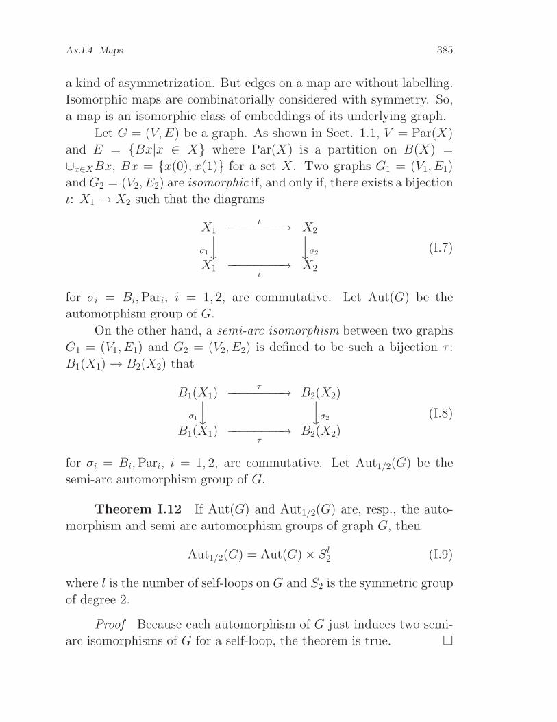
Ax.I.4 Maps 385
a kind of asymmetrization. But edges on a map are without labelling.
Isomorphic maps are combinatorially considered with symmetry. So,
a map is an isomorphic class of embeddings of its underlying graph.
Let G = (V,E) be a graph. As shown in Sect. 1.1, V = Par(X)
and E = Bx|x ∈ X where Par(X) is a partition on B(X) =
∪x∈XBx, Bx = x(0), x(1) for a set X. Two graphs G1 = (V1, E1)
andG2 = (V2, E2) are isomorphic if, and only if, there exists a bijection
ι: X1 → X2 such that the diagrams
X1ι−−−−−−−−→ X2
σ1
yyσ2
X1 −−−−−−−−→ι
X2
(I.7)
for σi = Bi,Pari, i = 1, 2, are commutative. Let Aut(G) be the
automorphism group of G.
On the other hand, a semi-arc isomorphism between two graphs
G1 = (V1, E1) and G2 = (V2, E2) is defined to be such a bijection τ :
B1(X1)→ B2(X2) that
B1(X1)τ−−−−−−−−→ B2(X2)
σ1
yyσ2
B1(X1) −−−−−−−−→τ
B2(X2)
(I.8)
for σi = Bi,Pari, i = 1, 2, are commutative. Let Aut1/2(G) be the
semi-arc automorphism group of G.
Theorem I.12 If Aut(G) and Aut1/2(G) are, resp., the auto-
morphism and semi-arc automorphism groups of graph G, then
Aut1/2(G) = Aut(G)× Sl2 (I.9)
where l is the number of self-loops on G and S2 is the symmetric group
of degree 2.
Proof Because each automorphism of G just induces two semi-
arc isomorphisms of G for a self-loop, the theorem is true.

386 Appendix I Concepts of Polyhedra and Maps
For map M = (Xα,β,P), its automorphisms are discussed with
asymmetrization in Chapter VIII. LetM(G) be the set of all noniso-
morphic maps with underlying graph G.
Lemma I.11 For an automorphism ζ on mapM = (Xα,β(X),P),
we have exhaustively ζ|B(X) ∈ Aut1/2(G) and ζα|B(X) ∈ Aut1/2(G)
where G = G(M), the underlying graph of M , and B(X) = X + βX.
Proof Because Xα,β(X) = (X + βX) + (αX +αβX) = B(X) +
αB(X), by Conjugate Axiom each ζ ∈ Aut(M) has exhaustively two
possibilities: ζ|B(X) ∈ Aut1/2(G) and ζα|B(X) ∈ Aut1/2(G).
Theorem I.13 Let Eg(G) be the set of all embeddings of a
graph G on a surface of genus g(orientable or nonorientable), then the
number of nonisomorphic maps in Eg(G) is
mg(G) =1
2× aut1/2(G)
∑
τ∈Aut1/2(G)
|Φ(τ)| (I.10)
where Φ(τ) = M ∈ Eg(G)|τ(M) = M or τα(M) = M.
Proof Suppose X1, X2, · · ·, Xm are all the equivalent classes of
X = Eg(G) under the group Aut1/2(G)× 〈α〉, then m = mg(G). Let
S(x) = τ ∈ Aut1/2(G)× 〈α〉| τ(x) = x
be the stabilizer at x, a subgroup of Aut1/2(G)×〈α〉. Because |Aut1/2(G)×〈α〉| = |S(xi)||Xi|, xi ∈ Xi, i = 1, 2, · · · , m, we have
m|Aut1/2(G)× 〈α〉| =m∑
i=1
|S(xi)||Xi|. (1)
By observing |S(xi)| independent of the choice of xi in the class Xi,

Ax.I.4 Maps 387
the right hand side of (1) is∑
x∈X|S(x)| =
∑
x∈X
∑
τ∈S(x)
1
=∑
τ∈Aut1/2(G)×〈α〉
∑
x=τ(x)
1
=∑
τ∈Aut1/2(G)×〈α〉|Φ(τ)|.
(2)
From (1) and (2), the theorem can be soon derived.
The theorem above shows how to find nonisomorphic super maps
of a graph when the automorphism group of the graph is known.
Theorem I.14 For a graph G, let Rg(G) and Eg(G) be, respec-
tively, the sets of all nonisomorphic rooted super maps and all distinct
embeddings of G with size ǫ(G) on a surface of genus g(orientable or
nonorientable). Then,
|Rg(G)| = 2ǫ(G)
aut1/2(G)|Eg(G)|. (I.11)
Proof Let Mg(G) be the set of all nonisomorphic super maps
of G. By (11.3),
|Rg(G)| = 4ǫ(G)
2× aut1/2(G)
∑
M∈Mg(G)
2× aut1/2(G)
aut(M).
By considering that
2× aut1/2(G) = |Aut1/2(G)× 〈α〉|= |(Aut1/2(G)× 〈α〉)|M | × |Aut1/2(G)× 〈α〉(M)|
and (Aut1/2(G)× 〈α〉)|M = Aut(M), we have
|Rg(G)| = 4ǫ(G)
|Aut1/2(G)× 〈α〉|∑
M∈Mg(G)
|Aut1/2(G)× 〈α〉(M)|
=2ǫ(G)
aut1/2(G)|Eg(G)|.

388 Appendix I Concepts of Polyhedra and Maps
This is (I.11).
This theorem enables us to determine all the super rooted maps
of a graph when the automorphism group of the graph is known. How-
ever, the problem of finding an automorphism of a graph is much more
difficult than that of finding an automorphism of a map on the basis
of Chapter VIII in general. For asymmetric graphs the two theo-
rems above provide results much simpler. More results are referred to
[MLW1].
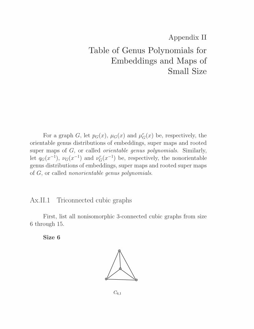
Appendix II
Table of Genus Polynomials forEmbeddings and Maps of
Small Size
For a graph G, let pG(x), µG(x) and µrG(x) be, respectively, the
orientable genus distributions of embeddings, super maps and rooted
super maps of G, or called orientable genus polynomials. Similarly,
let qG(x−1), νG(x−1) and νrG(x−1) be, respectively, the nonorientable
genus distributions of embeddings, super maps and rooted super maps
of G, or called nonorientable genus polynomials.
Ax.II.1 Triconnected cubic graphs
First, list all nonisomorphic 3-connected cubic graphs from size
6 through 15.
Size 6
C6,1

390 Appendix II Table of Genus Polynomials for Embeddings and Maps
Size 9
C9,1 C9,2
Size 12
C12,1 C12,2
C12.3 C12,4
Size 15
C15,1 C15,2 C15,3
C15,4 C15,5 C15,6

Ax.II.1 Triconnected cubic graphs 391
C15,7 C15,8 C15,9
C15,10 C15,11 C15,12
C15,13 C15,14
In what follows, the orientable and nonorientable genus poly-
nomials of embeddings, super maps and rooted super maps of 3-
connected cubic graphs shown above are provided.
Case of size 6:
Orientable
pC6,1(x) = 2 + 14x,
µC6,1(x) = 1 + 2x,
µrC6,1
(x) = 1 + 7x.
Nonorientable
qC6,1(x−1) = 14x+ 42x2 + 56x3,
νC6,1(x−1) = 2x+ 3x2 + 3x3,
νrC6,1
(x−1) = 7x+ 21x2 + 28x3.

392 Appendix II Table of Genus Polynomials for Embeddings and Maps
Case of size 9:
Orientable
pC9,1(x) = 2 + 38x+ 24x2,
µC9,1(x) = 1 + 5x+ 2x2,
µrC9,1
(x) = 3 + 57x+ 36x2;
pC9,2(x) = 40x+ 24x2,
µC9,2(x) = 2x+ x2,
µrC9,2
(x) = 10x+ 6x2.
Nonorientable
qC9,1(x−1) = 22x+ 122x2 + 424x3 + 392x4,
νC9,1(x−1) = 3x+ 12x2 + 28x3 + 23x4,
νrC9,1
(x−1) = 33x+ 183x2 + 636x3 + 588x4;
qC9,2(x−1) = 12x+ 108x2 + 432x3 + 408x4,
νC9,2(x−1) = x+ 2x2 + 6x3 + 6x4;
νrC9,2
(x−1) = 3x+ 27x2 + 108x3 + 102x4.
Case of size 12:
Orientable
pC12,1(x) = 2 + 70x+ 184x2,
µC12,1(x) = 1 + 15x+ 28x2,
µrC12,1
(x) = 12 + 420x+ 1104x2;

Ax.II.1 Triconnected cubic graphs 393
pC12,2(x) = 64x+ 192x2,
µC12,2(x) = 4x+ 12x2,
µrC12,2
(x) = 128x+ 384x2;
pC12,3(x) = 56x+ 200x2,
µC12,3(x) = 5x+ 13x2,
µrC12,3
(x) = 84x+ 300x2;
pC12,4(x) = 2 + 54x+ 200x2,
µC12,4(x) = 1 + 5x+ 8x2,
µrC12,4
(x) = 1 + 27x+ 100x2.
Nonorientable
qC12,1(x−1) = 30x+ 242x2 + 1448x3 + 3272x4 + 2944x5,
νC12,1(x−1) = 7x+ 44x2 + 217x3 + 452x4 + 38x5,
νrC12,1
(x−1) = 180x+ 1452x2 + 8688x3 + 19632x4 + 17664x5;
qC12,2(x−1) = 12x+ 180x2 + 1360x3 + 3312x4 + 3072x5,
νC12,2(x−1) = x+ 9x2 + 64x3 + 149x4 + 137x5,
νrC12,2
(x−1) = 24x+ 360x2 + 2720x3 + 6624x4 + 6144x5;
qC12,3(x−1) = 10x+ 158x2 + 1272x3 + 3296x4 + 3200x5,
νC12,3(x−1) = 2x+ 11x2 + 57x3 + 133x4 + 118x5;
νrC12,3
(x−1) = 15x+ 237x2 + 1908x3 + 2944x4 + 4800x5;
qC12,4(x−1) = 24x+ 192x2 + 1288x3 + 3264x4 + 3168x5,
νC12,4(x−1) = x+ 7x2 + 24x3 + 58x4 + 40x5;
νrC12,4
(x−1) = 12x+ 96x2 + 644x3 + 1632x4 + 1584x5.
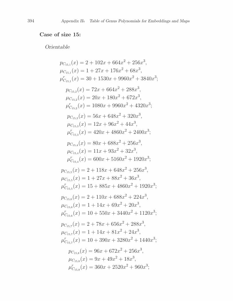
394 Appendix II Table of Genus Polynomials for Embeddings and Maps
Case of size 15:
Orientable
pC15,1(x) = 2 + 102x+ 664x2 + 256x3,
µC15,1(x) = 1 + 27x+ 176x2 + 68x3,
µrC15,1
(x) = 30 + 1530x+ 9960x2 + 3840x3;
pC15,2(x) = 72x+ 664x2 + 288x3,
µC15,2(x) = 20x+ 180x2 + 672x3,
µrC15,2
(x) = 1080x+ 9960x2 + 4320x3;
pC15,3(x) = 56x+ 648x2 + 320x3,
µC15,3(x) = 12x+ 96x2 + 44x3,
µrC15,3
(x) = 420x+ 4860x2 + 2400x3;
pC15,4(x) = 80x+ 688x2 + 256x3,
µC15,4(x) = 11x+ 93x2 + 32x3,
µrC15,4
(x) = 600x+ 5160x2 + 1920x3;
pC15,5(x) = 2 + 118x+ 648x2 + 256x3,
µC15,5(x) = 1 + 27x+ 88x2 + 36x3,
µrC15,5
(x) = 15 + 885x+ 4860x2 + 1920x3;
pC15,6(x) = 2 + 110x+ 688x2 + 224x3,
µC15,6(x) = 1 + 14x+ 69x2 + 20x3,
µrC15,6
(x) = 10 + 550x+ 3440x2 + 1120x3;
pC15,7(x) = 2 + 78x+ 656x2 + 288x3,
µC15,7(x) = 1 + 14x+ 81x2 + 24x3,
µrC15,7
(x) = 10 + 390x+ 3280x2 + 1440x3;
pC15,8(x) = 96x+ 672x2 + 256x3,
µC15,8(x) = 9x+ 49x2 + 18x3,
µrC15,8
(x) = 360x+ 2520x2 + 960x3;

Ax.II.1 Triconnected cubic graphs 395
pC15,9(x) = 48x+ 656x2 + 320x3,
µC15,9(x) = 8x+ 59x2 + 25x3,
µrC15,9
(x) = 180x+ 2460x2 + 1200x3;
pC15,10(x) = 88x+ 648x2 + 288x3,
µC15,10(x) = 5x+ 31x2 + 16x3,
µrC15,10
(x) = 220x+ 1620x2 + 720x3;
pC15,11(x) = 2 + 70x+ 632x2 + 320x3,
µC15,11(x) = 1 + 5x+ 28x2 + 10x3,
µrC15,11
(x) = 3 + 105x+ 948x2 + 480x3;
pC15,12(x) = 72x+ 632x2 + 320x3,
µC15,12(x) = 6x+ 24x2 + 14x3,
µrC15,12
(x) = 108x+ 948x2 + 480x3;
pC15,13(x) = 48x+ 720x2 + 256x3,
µC15,13(x) = 2x+ 15x2 + 6x3,
µrC15,13
(x) = 30x+ 450x2 + 160x3;
pC15,14(x) = 40x+ 664x2 + 320x3,
µC15,14(x) = x+ 7x2 + 2x3,
µrC15,14
(x) = 10x+ 166x2 + 80x3.
Nonorientable
qC15,1(x−1) = 38x+ 394x2 + 3336x3 + 12744x4 + 27008x5
+ 20992x6,
νC15,1(x−1) = 10x+ 104x2 + 838x3 + 3220x4 + 6768x5 + 5300x6;
νrC15,1
(x−1) = 570x+ 5910x2 + 50040x3 + 191160x4 + 405120x5
+ 314880x6;

396 Appendix II Table of Genus Polynomials for Embeddings and Maps
qC15,2(x−1) = 10x+ 214x2 + 2576x3 + 11664x4 + 27424x5
+ 22624x6,
νC15,2(x−1) = 4x+ 60x2 + 676x3 + 2988x4 + 6952x5 + 5688x6;
νrC15,2
(x−1) = 150x+ 3210x2 + 38640x3 + 174960x4 + 411360x5
+ 339360x6;
qC15,3(x−1) = 6x+ 158x2 + 2188x3 + 10912x4 + 27504x5
+ 23744x6,
νC15,3(x−1) = 2x+ 27x2 + 313x3 + 1466x4 + 3572x5 + 3044x6;
νrC15,3
(x−1) = 45x+ 1185x2 + 16410x3 + 81840x4 + 206280x5
+ 178080x6;
qC15,4(x−1) = 12x+ 244x2 + 2816x3 + 12224x4 + 27456x5
+ 21760x6,
νC15,4(x−1) = 2x+ 33x2 + 368x3 + 1565x4 + 3480x5 + 2736x6;
νrC15,4
(x−1) = 90x+ 1830x2 + 21120x3 + 91680x4 + 205920x5
+ 163200x6;
qC15,5(x−1) = 38x+ 410x2 + 3496x3 + 12952x4 + 26880x5
+ 20736x6,
νC15,5(x−1) = 8x+ 76x2 + 524x3 + 1768x4 + 3460x5 + 2652x6;
νrC15,5
(x−1) = 385x+ 3075x2 + 26220x3 + 97140x4 + 201600x5
+ 155520x6;
qC15,6(x−1) = 38x+ 402x2 + 3448x3 + 13040x4 + 27072x5
+ 20512x6,
νC15,6(x−1) = 6x+ 44x2 + 319x3 + 1157x4 + 2354x5 + 1744x6;
νrC15,6
(x−1) = 190x+ 2010x2 + 17240x3 + 65200x4 + 135360x5
+ 102560x6;

Ax.II.1 Triconnected cubic graphs 397
qC15,7(x−1) = 32x+ 312x2 + 2800x3 + 11800x4 + 27200x5
+ 22368x6,
νC15,7(x−1) = 5x+ 35x2 + 267x3 + 1077x4 + 2358x5 + 1866x6;
νrC15,7
(x−1) = 160x+ 1560x2 + 14000x3 + 59000x4 + 136000x5
+ 111840x6;
qC15,8(x−1) = 12x+ 260x2 + 2976x3 + 12432x4 + 27328x5
+ 21504x6,
νC15,8(x−1) = 2x+ 21x2 + 207x3 + 828x4 + 1772x5 + 1382x6;
νrC15,8
(x−1) = 45x+ 975x2 + 11160x3 + 26620x4 + 192480x5
+ 80640x6;
qC15,9(x−1) = 4x+ 132x2 + 2049x3 + 10720x4 + 27616x5
+ 24000x6,
νC15,9(x−1) = x+ 16x2 + 152x3 + 753x4 + 1811x5 + 1559x6;
νrC15,9
(x−1) = 15x+ 495x2 + 7650x3 + 40200x4 + 103560x5
+ 90000x6;
qC15,10(x−1) = 12x+ 252x2 + 2864x3 + 12136x4 + 27264x5
+ 21984x6,
νC15,10(x−1) = x+ 11x2 + 124x3 + 517x4 + 1154x5 + 941x6;
νrC15,10
(x−1) = 30x+ 630x2 + 7160x3 + 30340x4 + 681560x5
+ 54960x6;
qC15,11(x−1) = 30x+ 282x2 + 2560x3 + 11240x4 + 27168x5
+ 23232x6,
νC15,11(x−1) = 2x+ 17x2 + 92x3 + 351x4 + 754x5 + 624x6;
νrC15,11
(x−1) = 45x+ 423x2 + 3840x3 + 16860x4 + 40752x5
+ 34848x6;

398 Appendix II Table of Genus Polynomials for Embeddings and Maps
qC15,12(x−1) = 12x+ 220x2 + 2480x3 + 11240x4 + 27264x5
+ 23296x6,
νC15,12(x−1) = 2x+ 11x2 + 90x3 + 343x4 + 756x5 + 638x6;
νrC15,12
(x−1) = 18x+ 330x2 + 3720x3 + 16860x4 + 40896x5
+ 34944x6;
qC15,13(x−1) = 120x2 + 2232x3 + 11568x4 + 27936x5
+ 22656x6,
νC15,13(x−1) = 4x2 + 28x3 + 144x4 + 307x5 + 259x6;
νrC15,13
(x−1) = 75x2 + 1395x3 + 7230x4 + 17460x5
+ 14160x6;
qC15,14(x−1) = 4x+ 120x2 + 1900x3 + 10440x4 + 27664x5
+ 24384x6,
νC15,14(x−1) = x+ 2x2 + 16x3 + 62x4 + 142x5 + 111x6;
νrC15,14
(x−1) = x+ 30x2 + 474x3 + 2610x4 + 6916x5
+ 6039x6.
Ax.II.2 Bouquets
Let Bm be the bouquet of size m, m ≥ 1.
Case of m = 1:
Orientable
pB1(x) = 1,
µB1(x) = 1,
µrB1
(x) = 1.

Ax.II.2 Bouquets 399
Nonorientable
qB1(x−1) = x,
νB1(x−1) = x,
νrB1
(x−1) = x.
Case of m = 2:
Orientable
pB2(x) = 4 + 2x,
µB2(x) = 1 + x,
µrB2
(x) = 2 + x.
Nonorientable
qB2(x−1) = 10x+ 8x2,
νB2(x−1) = 2x+ 2x2,
νrB2
(x−1) = 5x+ 4x2.
Case of m = 3:
Orientable
pB3(x) = 40 + 80x,
µB3(x) = 2 + 3x,
µrB3
(x) = 5 + 10x.
Nonorientable
qB3(x−1) = 176x+ 336x2 + 328x3,

400 Appendix II Table of Genus Polynomials for Embeddings and Maps
νB3(x−1) = 5x+ 8x2 + 8x3,
νrB3
(x−1) = 22x+ 42x2 + 41x3.
Case of m = 4:
Orientable
pB4(x) = 672 + 3360x+ 1008x2,
µB4(x) = 3 + 10x+ 4x2,
µrB4
(x) = 14 + 70x+ 21x2.
Nonorientable
qB4(x−1) = 4464x+ 14592x2 + 33120x3 + 23424x4,
νB4(x−1) = 12x+ 33x2 + 64x3 + 47x4,
νrB4
(x−1) = 93x+ 304x2 + 690x3 + 488x4.
Case of m = 5:
Orientable
pB5(x) = 16128 + 161280x+ 185472x2,
µB5(x) = 6 + 35x+ 38x2,
µrB5
(x) = 42 + 420x+ 483x2.
Nonorientable
qB5(x−1) = 148224x+ 718080x2 + 2745600x3 + 4477440x4
+ 3159936x5,
νB5(x−1) = 33x+ 131x2 + 442x3 + 686x4 + 473x5,
νrB5
(x−1) = 386x+ 1870x2 + 7150x3 + 11660x4 + 8229x5.

Ax.II.3 Wheels 401
Case of m = 6:
Orientable
pB6(x) = 506880 + 8870400x+ 24837120x2 + 5702400x3,
µB6(x) = 12 + 132x+ 328x2 + 82x3,
µrB6
(x) = 132 + 2310x+ 6468x2 + 1485x3.
Ax.II.3 Wheels
Let Wn be the wheel of order n, n ≥ 4, i.e., all vertices are of
valency (or degree) 3 but one and all 3-valent vertices form a circuit.
Case of n = 4:
Orientable
pW4(x) = 2 + 14x,
µW4(x) = 1 + 2x,
µrW4
(x) = 1 + 7x.
Nonorientable
qW4(x−1) = 14x+ 42x2 + 56x3,
νW4(x−1) = 2x+ 3x2 + 3x3,
νrW4
(x−1) = 7x+ 21x2 + 28x3.
Case of n = 5:
Orientable
pW5(x) = 2 + 58x+ 36x2,
µW5(x) = 1 + 8x+ 4x2,
µrW5
(x) = 4 + 116x+ 72x2.

402 Appendix II Table of Genus Polynomials for Embeddings and Maps
Nonorientable
qW5(x−1) = 28x+ 176x2 + 640x3 + 596x4,
νW5(x−1) = 4x+ 18x2 + 52x3 + 48x4,
νrW5
(x−1) = 56x+ 352x2 + 1280x3 + 1192x4.
Case of n = 6:
Orientable
pW6(x) = 2 + 190x+ 576x2,
µW6(x) = 1 + 14x+ 41x2,
µrW6
(x) = 4 + 380x+ 1152x2.
Nonorientable
qW6(x−1) = 52x+ 580x2 + 4080x3 + 9880x4 + 9216x5,
νW6(x−1) = 6x+ 38x2 + 227x3 + 539x4 + 494x5,
νrW6
(x−1) = 104x+ 1160x2 + 8160x3 + 19760x4 + 18432x5.
Case of n = 7:
Orientable
pW7(x) = 2 + 550x+ 4968x2 + 2160x3,
µW7(x) = 1 + 34x+ 240x2 + 106x3,
µrW7
(x) = 4 + 1100x+ 9936x2 + 4320x3.
Nonorientable
qW7(x−1) = 94x+ 1680x2 + 19482x3 + 87536x4 + 205496x5
+ 169552x6,

Ax.II.4 Link bundles 403
νW7(x−1) = 8x+ 89x2 + 878x3 + 3829x4 + 8788x5 + 7241x6,
νrW7
(x−1) = 188x+ 3360x2 + 38964x3 + 175072x4 + 410992x5
+ 339104x6.
Case of order n = 8:
Orientable
pW8(x) = 2 + 1484x+ 31178x2 + 59496x3,
µW8(x) = 1 + 63x+ 1176x2 + 2246x3,
µrW8
(x) = 4 + 2968x+ 62356x2 + 118992x3.
Ax.II.4 Link bundles
Let Lm be the link bundle of size m, m ≥ 3. A link bundle is a
graph of order 2 without loop.
Case of size m = 3:
Orientable
pL3(x) = 2 + 2x,
µL3(x) = 1 + x,
µrL3
(x) = 1 + 1x.
Nonorientable
qL3(x−1) = 6x+ 6x2,
νL3(x−1) = 1x+ 2x2,
νrL3
(x−1) = 3x+ 3x2.

404 Appendix II Table of Genus Polynomials for Embeddings and Maps
Case of size m = 4:
Orientable
pL4(x) = 6 + 30x,
µL4(x) = 1 + 2x,
µrL4
(x) = 1 + 5x.
Nonorientable
qL4(x−1) = 36x+ 96x2 + 120x3,
νL4(x−1) = 2x+ 4x2 + 3x3,
νrL4
(x−1) = 6x+ 16x2 + 20x3.
Case of size m = 5:
Orientable
pL5(x) = 24 + 360x+ 192x2,
µL5(x) = 1 + 3x+ 3x2,
µrL5
(x) = 1 + 15x+ 8x2.
Nonorientable
qL5(x−1) = 240x+ 1200x2 + 3840x3 + 3360x4,
νL5(x−1) = 2x+ 7x2 + 14x3 + 14x4,
νrL5
(x−1) = 10x+ 50x2 + 160x3 + 140x4.
Case of size m = 6:
Orientable
pL6(x) = 120 + 4200x+ 10080x2,
µL6(x) = 1 + 6x+ 10x2,
µrL6
(x) = 1 + 35x+ 84x2.

Ax.II.5 Complete bipartite graphs 405
Nonorientable
qL6(x−1) = 1800x+ 14400x2 + 84120x3 + 184320x4 + 161760x5,
νL6(x−1) = 3x+ 14x2 + 48x3 + 96x4 + 72x5,
νrL6
(x−1) = 15x+ 120x2 + 701x3 + 1536x4 + 1348x5.
Case of size m = 7:
Orientable
pL7(x) = 720 + 50400x+ 337680x2 + 129600x3,
µL7(x) = 1 + 8x+ 31x2 + 16x3,
µrL7
(x) = 1 + 70x+ 469x2 + 180x3.
Ax.II.5 Complete bipartite graphs
Let Km,n be the complete bipartite graph of order m+n, m,n ≥3.
Case of order m+ n = 6:
Orientable
pK3,3(x) = 40x+ 24x2,
µK3,3(x) = 2x+ x2,
µrK3,3
(x) = 10x+ 6x2.
Nonorientable
qK3,3(x−1) = 12x+ 108x2 + 432x3 + 408x4,
νK3,3(x−1) = x+ 2x2 + 6x3 + 6x4,
νrK3,3
(x−1) = 3x+ 27x2 + 108x3 + 102x4.

406 Appendix II Table of Genus Polynomials for Embeddings and Maps
Case of order m+ n = 7:
Orientable
pK3,4(x) = 156x+ 2244x2 + 1056x3,
µK3,4(x) = 3x+ 16x2 + 10x3,
µrK3,4
(x) = 26x+ 374x2 + 176x3.
Nonorientable
qK3,4(x−1) = 12x+ 432x2 + 6852x3 + 36288x4 + 93360x5
+ 80784x6,
νK3,4(x−1) = x + 4x2 + 33x3 + 156x4 + 358x5 + 317x6,
νrK3,4
(x−1) = 2x+ 72x2 + 1142x3 + 6048x4 + 15560x5
+ +13464x6.
Case of order m+ n = 8:
Orientable
pK4,4(x) = 108x+ 24984x2 + 565020x3 + 1089504x4,
µK4,4(x) = 2x+ 25x2 + 318x3 + 530x4,
µrK4,4
(x) = 3x+ 694x2 + 15695x3 + 30264x4.
pK3,5(x) = 240x+ 37584x2 + 290880x3 + 113664x4,
µK3,5(x) = x+ 33x2 + 225x3 + 105x4,
µrK3,5
(x) = 10x+ 1566x2 + 12120x3 + 4736x4.

Ax.II.6 Complete graphs 407
Ax.II.6 Complete graphs
Let Kn be the complete graph of order n, n ≥ 4.
Case of order n = 4:
Because of K4 = W4, seen from Case of order n = 4 in Ax.II.3.
Case of order n = 5:
Orientable
pK5(x) = 462x+ 4974x2 + 3240x3,
µK5(x) = 6x+ 31x2 + 13x3,
µrK5
(x) = 77x+ 829x2 + 390x3.
Nonorientable
qK5(x−1) = 54x+ 1320x2 + 17490x3 + 84660x4
+ +208776x5 + 177588x6,
νK5(x−1) = 2x+ 11x2 + 99x3 + 417x4 + 955x5 + 796x6,
νrK5
(x−1) = 9x+ 220x2 + 2915x3 + 14110x4 + 34796x5
+ +29598x6.
Case of order n = 6:
Orientable
pK6(x) = 1800x+ 654576x2 + 24613800X3
+ +124250208x4 + 41582592x5.

408 Appendix II Table of Genus Polynomials for Embeddings and Maps
Nonorientable
qK6(x−1) = 24x+ 4560x2 + 370920x3 + 10828440x4
+ 192264576x5 + 1927543032x6 + 11905560960x7
+ 42386101920x8 + 79831388160x9
+ 59244281856x10.

Appendix III
Atlas of Rooted and Unrooted Mapsfor Small Graphs
In the symbol X : a, b, c for a map appearing under a figure
below, X is the under graph of the map, a = oy or qy are, respectively,
orientable or nonorientable genus y, b is the series number with two
digits and c is the number of ways to assign a root. And, x on a
surface is for x−1, or −x, x = 1, 2, · · ·.
Ax.III.1 Bouquets Bm of size 4 ≥ m ≥ 1
Case m = 1:
Orientable genus 0 R1
16B1 : o0− 01− 01
Nonorientable genus 1
R1 1
6B1 : q1− 01− 01

410 Appendix III Atlas of Rooted and Unrooted Maps
Case m = 2:
Orientable genus 0 -6?
1
1
2
2 6-B2 : o0− 01− 02
Orientable genus 1 -66-
1
2
1
2 6B2 : o1− 01− 01
Nonorientable genus 1-?
6-
1
2
2
1 6-? -?
6-
1
2
1
2 6B2 : q1− 01− 04 B2 : q1− 02− 01

Ax.III.1 Bouquets Bm of size 4 ≥ m ≥ 1 411
Nonorientable genus 2-?
6
1
1
2
2 6- -?
6-
1
2
1
2 6-B2 : q2− 01− 02 B2 : q2− 02− 02
Case m = 3:
Orientable genus 0
1
1
2
2
3
3 6* 1
2
2
1
3
3 6*sB3 : o0− 01− 02 B3 : o0 − 02− 03
Orientable genus 1
1
2
1
2
3
3 6*j? 1
3
2
3
1
2 6*j 1
2
3
1
2
3 6*jB3 : o1 − 01− 04 B3 : o1− 02− 03 B3 : o1− 03− 03

412 Appendix III Atlas of Rooted and Unrooted Maps
Nonorientable genus 1
16*j 1
2
2
3
3 ?+i 16j 1
2
3
2
3 ?i 16j 1
2
3
3
2 ?iB3 : q1− 01− 06 B3 : q1− 02− 06 B3 : q1− 03− 06
16j 1
2
3
3
2
16 2
3
1
2
3
B3 : q1− 04− 03 B3 : q1− 05− 01
Nonorientable genus 2
16j 1
2
2
3
3 ?+i 1
1
2
3
2
3
16j 1
2
3
2
3 ?iB3 : q2− 01− 06 B3 : q2− 02− 12 B3 : q2− 03− 06
16j 2
3
3
2
1 ?i 16j 1
2
3
3
2
16j 2
1
3
2
3
B3 : q2− 04− 06 B3 : q2− 05− 03 B3 : q2− 06− 03

Ax.III.1 Bouquets Bm of size 4 ≥ m ≥ 1 413
16*j 2
1
3
2
3
16j 2
3
1
2
3
B3 : q2− 07− 03 B3 : q2− 08− 03
Nonorientable genus 3
16 1
2
2
3
3
16*j 1
2
3
2
3 ?i 1
1
2
3
2
3
B3 : q3− 01− 02 B3 : q3− 02− 06 B3 : q3− 03− 12
1
1
2
3
3
2 6j 16 2
1
3
2
3 j?Y 16j 2
1
3
2
3 ?YB3 : q3− 04− 03 B3 : q3− 05− 06 B3 : q3− 06− 06
16j 2
1
3
2
3
16j 2
3
1
2
3
B3 : q3− 07− 03 B3 : q3− 08− 03
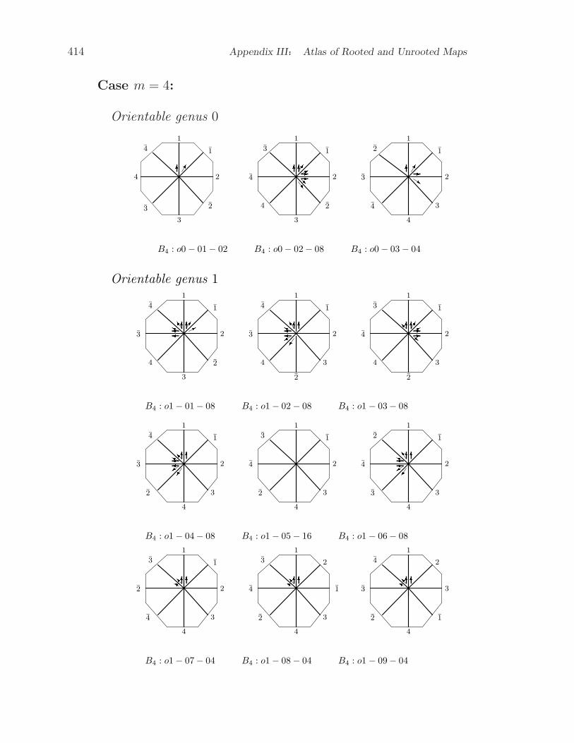
414 Appendix III Atlas of Rooted and Unrooted Maps
Case m = 4:
Orientable genus 0
1
1
2
2
3
3
4
4 6 1
1
2
2
3
4
4
3 66*--R 1
1
2
3
4
4
3
2 6-sB4 : o0 − 01− 02 B4 : o0− 02− 08 B4 : o0− 03− 04
Orientable genus 11
1
2
2
3
4
3
4 Y66* 1
1
2
3
2
4
3
4 +Y66 1
1
2
3
2
4
4
3 I66*--RB4 : o1− 01− 08 B4 : o1− 02− 08 B4 : o1 − 03− 08
1
1
2
3
4
2
3
4 66IY+ 1
1
2
3
4
2
4
3
1
1
2
3
4
3
4
2 66Y+B4 : o1− 04− 08 B4 : o1− 05− 16 B4 : o1 − 06− 08
1
1
2
3
4
2
4
3 66IY 1
2
1
3
4
2
4
3 66IY 1
2
3
1
4
2
3
4 66IYB4 : o1− 07− 04 B4 : o1− 08− 04 B4 : o1 − 09− 04

Ax.III.2 Link bundles Lm, 7 ≥ m ≥ 3 415
1
2
3
1
4
3
2
4 66B4 : o1− 10− 02
Orientable genus 2
1
2
1
2
3
4
3
4 66* 1
2
1
3
2
4
3
4 66*-RU- 1
2
1
3
4
2
3
4 Y66B4 : o2− 01− 04 B4 : o2− 02− 08 B4 : o2 − 03− 08
61 2
3
4
1
2
3
4
B4 : o2− 04− 01
Ax.III.2 Link bundles Lm, 6 ≥ m ≥ 3
Case m = 3:
Orientable genus 0

416 Appendix III Atlas of Rooted and Unrooted Maps-6?
1
12
2
L3 : o0 − 01− 01
Orientable genus 1 -6?
1
1
2 2
L3 : o1 − 01− 01
Nonorientable genus 1 -6?
1
2
1
2U?L3 : q1− 01− 03
Nonorientable genus 2

Ax.III.2 Link bundles Lm, 7 ≥ m ≥ 3 417-6?
1
2 N1
2
L3 : q2− 01− 03
Case m = 4:
Orientable genus 0
1
2
363
2
1
L4 : o0 − 01− 01
Orientable genus 1
1
2
361
2
3
1
2
366??1
3
2
L4 : o1− 01− 01 L4 : o1 − 02− 04

418 Appendix III Atlas of Rooted and Unrooted Maps
Nonorientable genus 1
1
2
3662
3
1
1
2
36*-?
1
2
3
L4 : q1− 01− 02 L4 : q1− 02− 04
Nonorientable genus 2
1
2
3 661
3
2
1
2
3 661-??i1
3
2
1
2
3 611
2
3
L4 : q2− 01− 02 L4 : q2− 02− 08 L4 : q2− 03− 02
1
2
3661-1
2
3
L4 : q2− 04− 04
Nonorientable genus 3

Ax.III.2 Link bundles Lm, 7 ≥ m ≥ 3 419
1
2
3
)??661-1
3
2
1
2
3 661-??i1
3
2
1
2
3 6611
2
3
L4 : q3− 01− 08 L4 : q3− 02− 08 L4 : q3− 03− 04
Case m = 5:
Orientable genus 0
1
2
3
4 Æ4
3
2
1
L5 : o0 − 01− 01
Orientable genus 1
1
2
3
4 ÆNUjj2
1
4
3
1
2
3
4 ÆN1
4
3
2
1
2
3
4 Æj1
2
4
3
L5 : o1− 01− 05 L5 : o1− 02− 05 L5 : o1 − 03− 05
Orientable genus 2

420 Appendix III Atlas of Rooted and Unrooted Maps
1
2
3
4 Æ2
4
1
3
1
2
3
4 Æjj1
3
4
2
1
2
3
4 Æ1
2
3
4
L5 : o2− 01− 02 L5 : o2− 02− 05 L5 : o2 − 03− 01
Nonorientable genus 1
1
2
3
4 ÆN2
3
4
1
1
2
3
4 Æjj1
2
3
4
L5 : q1− 01− 05 L5 : q1− 02− 05
Nonorientable genus 2
1
2
3
4 ÆjjU62
4
3
1
1
2
3
4 Æ Æ-qNiI1
4
3
2
1
2
3
4 Æ-jUNYY1
3
4
2
L5 : q2− 01− 05 L5 : q2− 02− 10 L5 : q2− 03− 10
1
2
3
4 Æ qjUN1
3
2
4
1
2
3
4 Æ-jNYY1
2
4
3
1
2
3
4 ÆjqY1
2
3
4
L5 : q2− 04− 05 L5 : q2− 05− 10 L5 : q2− 06− 05
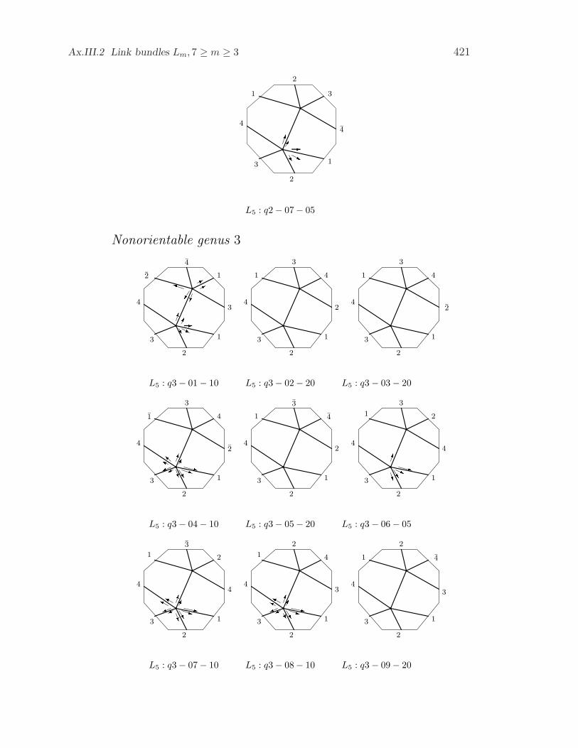
Ax.III.2 Link bundles Lm, 7 ≥ m ≥ 3 421
1
2
3
4 Æ -jU1
2
3
4
L5 : q2− 07− 05
Nonorientable genus 3
1
2
3
4 Æ **-jUi2
4
1
3
1
2
3
4
3
1 4
2
1
2
3
4
3
1 4
2
L5 : q3− 01− 10 L5 : q3− 02− 20 L5 : q3− 03− 20
1
2
3
4 Æ zqNYI1
3
4
2
1
2
3
4
1
3
4
2
1
2
3
4 Æ zjN1
3
2
4
L5 : q3− 04− 10 L5 : q3− 05− 20 L5 : q3− 06− 05
1
2
3
4 Æ zqNYY1
3
2
4
1
2
3
4 Æ zqUYY1
2
4
3
1
2
3
4
1
2
4
3
L5 : q3− 07− 10 L5 : q3− 08− 10 L5 : q3− 09− 20

422 Appendix III Atlas of Rooted and Unrooted Maps
1
2
3
4 Æ zjNYI1
2
4
3
1
2
3
4 Æ zjNYI1
2
4
3
1
2
3
4 Æ-1
2
4
3
L5 : q3− 10− 10 L5 : q3− 11− 10 L5 : q3− 12− 05
1
2
3
4 Æ-j4
1
2
3
1
2
3
4 ÆY -j4
1
2
3
L5 : q3− 13− 05 L5 : q3− 14− 05
Nonorientable genus 4
1
2
3
4 ÆiqY -iM js2
4
1
3
1
2
3
4 Æ-j iiM62
4
1
3
1
2
3
4 Æ-jUYY1
3
4
2
L5 : q4− 01− 10 L5 : q4− 02− 10 L5 : q4− 03− 10
1
2
3
4 Æ ÆjjUUYY1
3
4
2
1
2
3
4 Æ-jM 6**s1
3
4
2
1
2
3
4 Æ Æ-j1
3
4
2
sM M**L5 : q4− 04− 10 L5 : q4− 05− 10 L5 : q4− 06− 10

Ax.III.2 Link bundles Lm, 7 ≥ m ≥ 3 423
1
2
3
4 Æ-j1
3
4
2
1
2
3
4
1
3
4
2
1
2
3
4 Æ-qUYY1
2
4
3
L5 : q4− 07− 05 L5 : q4− 08− 20 L5 : q4− 09− 10
1
2
3
4 Æ-1
2
4
3
1
2
3
4 Æ-1
2
4
3
1
2
3
4
1
2
4
3
L5 : q4− 10− 05 L5 : q4− 11− 05 L5 : q4− 12− 20
1
2
3
4 Æ jU-YI1
2
4
3
1
2
3
4 Æ-YI1
2
3
4
L5 : q4− 13− 10 L5 : q4− 14− 05
Case m = 6:
Orientable genus 0

424 Appendix III Atlas of Rooted and Unrooted Maps
1
23
4
5
5
4
32
16L6 : o0− 01− 01
Orientable genus 1
1
23
4
5 663
25
4
1
1
23
4
5 661-jj??ii2
15
4
3
1
23
4
5 61-2
13
5
4
L6 : o1− 01− 02 L6 : o1− 02− 12 L6 : o1 − 03− 03
1
23
4
5 66jj??1
54
3
2
1
23
4
5 66jj??1
32
5
4
1
23
4
5 661i1
25
4
3
L6 : o1− 04− 06 L6 : o1− 05− 06 L6 : o1 − 06− 06
Orientable genus 2

Ax.III.2 Link bundles Lm, 7 ≥ m ≥ 3 425
1
23
4
5
66**66jj??2
5
1
4
3
1
23
4
5 661-ji2
41
5
3
1
23
4
5 66j1
5
34
2
L6 : o2− 01− 12 L6 : o2− 02− 06 L6 : o2 − 03− 03
1
23
4
5 661-jj1
45
3
2
1
23
4
5 661
45
2
3
1
23
4
5
1
35
4
2
L6 : o2− 04− 06 L6 : o2− 05− 02 L6 : o2 − 03− 24
1
23
4
5
iY6666jj??1
35
2
4
1
23
4
5 661-jj??ii1
24
5
3
1
23
4
5 661-1
2
3
5
4
L6 : o2− 07− 12 L6 : o2− 08− 12 L6 : o2 − 09− 06
1
23
4
5 61
23
4
5
L6 : o2− 01− 01
Case m = 7:

426 Appendix III Atlas of Rooted and Unrooted Maps
Orientable genus 0
1
2
34
5
6
6
5
4 3
2
16L7 : o0− 01− 01
Orientable genus 1
1
2
34
5
6
1
2
6 5
4
366UU * 1
2
34
5
6
1
3
2 6
5
466*1jjUU66ii 1
2
34
5
6
1
6
5 4
3
266jjUUL7 : o1− 01− 07 L7 : o1− 02− 14 L7 : o1 − 03− 07
1
2
34
5
6
2
1
3 6
5
46611 1
2
34
5
6
2
1
4 3
6
5611jjUU 1
2
34
5
6
2
1
6 5
4
36611jjUUiiL7 : o1− 04− 07 L7 : o1− 05− 07 L7 : o1 − 06− 14

Ax.III.2 Link bundles Lm, 7 ≥ m ≥ 3 427
1
2
34
5
6
3
2
1 6
5
4611jjUU 1
2
34
5
6
3
2
6 5
4
16611L7 : o1− 07− 07 L7 : o1− 08− 07
Orientable genus 2
1
2
34
5
6
1
2
3 4
5
66611 q 1
2
34
5
6
1
2
3 6
5
46611 1
2
34
5
6
1
2
4 3
6
56611 UL7 : o2− 01− 07 L7 : o2− 02− 07 L7 : o2 − 03− 07
1
2
34
5
6
1
2
4 5
6
366*1jjU 1
2
34
5
6
1
2
4 6
5
3
1
2
34
5
6
1
2
5 6
4
36611jjUUi 6iL7 : o2− 04− 07 L7 : o2− 05− 28 L7 : o2 − 06− 14
1
2
34
5
6
1
2
46
5
366UU6 1 1
2
34
5
6
1
2
5
6
4
3 66jjUU6 1
2
34
5
6
1
3
2 5
6
4
L7 : o2− 07− 07 L7 : o2− 08− 07 L7 : o2 − 09− 28

428 Appendix III Atlas of Rooted and Unrooted Maps
1
2
34
5
6
1
3
5 2
6
46611jjUUii 1
2
34
5
6
1
3
5 4
6
26611jjUN ii 1
2
34
5
6
1
3
5 6
3
46611jjUi ??) 11L7 : o2− 10− 14 L7 : o2− 11− 14 L7 : o2 − 12− 14
1
2
34
5
6
1
3
6 2
5
4
1
2
34
5
6
1
3
6 5
2
4
1
2
34
5
6
1
3
6 5
4
2
L7 : o2− 13− 28 L7 : o2− 14− 28 L7 : o2 − 15− 28
1
2
34
5
6
1
4
3 6
5
26611jjUU)ii 1
2
34
5
6
1
4
6 5
2
36611jjUN )ii 1
2
34
5
6
1
4
6 5
3
2
L7 : o2− 16− 14 L7 : o2− 17− 14 L7 : o2 − 18− 28
1
2
34
5
6
1
5
6 4
3
26611jjU 1
2
34
5
6
1
6
3 5
4
26611jjUUii 1
2
34
5
6
1
6
4 5
3
26611jjiL7 : o2− 19− 07 L7 : o2− 20− 14 L7 : o2 − 21− 07

Ax.III.2 Link bundles Lm, 7 ≥ m ≥ 3 429
1
2
34
5
6
2
1
4 6
3
5
1
2
34
5
6
2
1
4 6
5
36611jjUN )ii 1
2
34
5
6
2
1
5 4
6
36611jjUU??iiL7 : o2− 22− 28 L7 : o2− 23− 14 L7 : o2 − 24− 14
1
2
34
5
6
2
4
1 6
5
36611j) ??) KKÆ1
2
34
5
6
2
5
1 3
6
46611 1
2
34
5
6
2
5
1 6
4
36611qjUU )iiL7 : o2− 25− 14 L7 : o2− 26− 07 L7 : o2 − 27− 14
1
2
34
5
6
2
5
4
6
1
36611qjUU )ii 1
2
34
5
6
2
6
1 5
4
366qjUN ??))ii1
2
34
5
6
2
6
5 1
4
36611U6N ??iiKKL7 : o2− 28− 14 L7 : o2− 29− 14 L7 : o2 − 30− 14

430 Appendix III Atlas of Rooted and Unrooted Maps
1
2
34
5
6
3
2
6 5
1
466jjUU??iiL7 : o2− 31− 14
Orientable genus 3
1
2
34
5
6
1
2
3 4
5
66 1
2
34
5
6
1
2
3 5
6
46611zjUU)ii 1
2
34
5
6
1
2
4 6
3
56611UN ??KMÆL7 : o3− 01− 01 L7 : o3− 02− 14 L7 : o3 − 03− 14
1
2
34
5
6
1
2
5 6
3
466UN 1 1
2
34
5
6
1
3
4 6
2
56611jj ?? 1
2
34
5
6
1
3
5 6
4
26611qjUN??) *1L7 : o3− 04− 07 L7 : o3− 05− 14 L7 : o3 − 06− 14

Ax.III.2 Link bundles Lm, 7 ≥ m ≥ 3 431
1
2
34
5
6
1
3
6 4
2
566jjUU??iiKK1
2
34
5
6
1
3
6 4
5
26611jjUUii 1
2
34
5
6
1
4
6 2
5
36611jjUN iiL7 : o3− 07− 14 L7 : o3− 08− 14 L7 : o3 − 09− 14
1
2
34
5
6
1
4
6 3
5
2
1
2
34
5
6
1
5
6 3
4
26611 j 1
2
34
5
6
2
4
1 6
3
56611jjUUiiKML7 : o3− 10− 28 L7 : o3− 11− 07 L7 : o3 − 12− 14
1
2
34
5
6
2
4
6 1
3
566 1
2
34
5
6
2
5
1 4
6
36611jjUU??)ii1
2
34
5
6
2
6
4 1
5
366UU 1L7 : o3− 13− 02 L7 : o3− 14− 14 L7 : o3 − 15− 07
1
2
34
5
6
3
6
2 5
1
466L7 : o3 − 16− 02

432 Appendix III Atlas of Rooted and Unrooted Maps
Ax.III.3 Complete bipartite graphs Km,n, 4 ≥ m,n ≥ 3
Case m+ n = 6:
Orientable genus 1
1
3
4
2
I--Y 6RR3
4
2
1
1
3
2
44
3
2
1
K3,3 : o1− 01− 09 K3,3 : o1 − 02− 01
Orientable genus 2
1
3
2
4 YRR3
4
2
1
K3,3 : o2− 01− 06
Nonorientable genus 1
1
3
4
2*4
3
1
2
K3,3 : q1− 01− 03
Nonorientable genus 2

Ax.III.3 Complete bipartite graphs Km,n, 4 ≥ m,n ≥ 3 433
1
3
4
2
YjR I-Y - 6RU3
4
2
1
1
3
2
4iRjIY
4
3
2
1
K3,3 : q2− 01− 18 K3,3 : q2− 02− 09
Nonorientable genus 3
1
3
4
2
YR I*-YRiRU4
3
2
1
1
3
2
4
YjY iRR I1-I3
4
2
1
1
3
2
43
4
2
1
K3,3 : q3− 01− 18 K3,3 : q3− 02− 18 K3,3 : q3− 03− 36
1
3
2
4
YRR I4
Y3
2
1
1
3
2
4
RR I-I - 6R4
3
2
1
1
3
2
4
RjI1-Y4
3
2
1
K3,3 : q3− 04− 09 K3,3 : q3− 05− 18 K3,3 : q3− 06− 09
Nonorientable genus 4
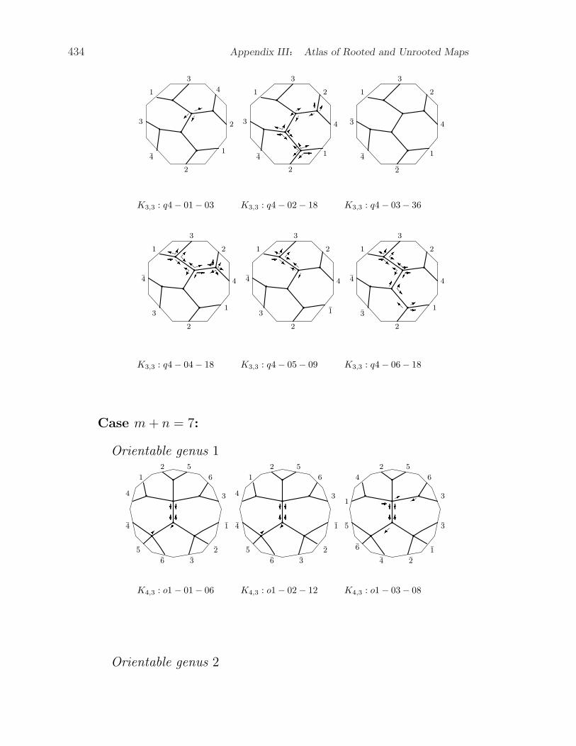
434 Appendix III Atlas of Rooted and Unrooted Maps
1
3
4
2
13
4
2
1
1
3
2
4
6*RiR K1I-3
4
2
1
1
3
2
43
4
2
1
K3,3 : q4− 01− 03 K3,3 : q4− 02− 18 K3,3 : q4− 03− 36
1
3
2
4
iRR I1-Y 6jU4
3
2
1
1
3
2
4
YRjIY4
3
2
1
1
3
2
4
I--YjYR RI*4 -3
2
1
K3,3 : q4− 04− 18 K3,3 : q4− 05− 09 K3,3 : q4− 06− 18
Case m+ n = 7:
Orientable genus 1
4
1
2 5
6
3??664
5
6 3
2
1
4
1
2 5
6
3??664
5
6 3
2
1
1
4
2 5
6
3??66* 5
6
4 2
1
3
K4,3 : o1 − 01− 06 K4,3 : o1− 02− 12 K4,3 : o1− 03− 08
Orientable genus 2

Ax.III.3 Complete bipartite graphs Km,n, 4 ≥ m,n ≥ 3 435
4
1
2 5
6
3?66
5
4 3
2
1
1
4
5 2
6
366RjK 6-j Y?? I*Y*R4
5
6 3
1
2
1
4
5 2
6
3??66jj IY5
4
6 3
1
2
K4,3 : o2 − 01− 02 K4,3 : o2− 02− 24 K4,3 : o2− 03− 12
1
4
5 2
6
3K6-j 66jj*RU YI*i??6
4
5 3
1
2
1
4
5 2
6
3Y??K6-j 66jR I*jjY 4
6
5 2
3
1
1
4
5 2
6
366*i-???? Y 66jR*RY6
4
5 2
3
1
K4,3 : o2 − 04− 24 K4,3 : o2− 05− 24 K4,3 : o2− 06− 24
1
4
5 2
6
3
4
5
6 3
2
1
Y??66js* 1
4
5 2
6
366jR??Y5
4
6
3
2
1
K6-jRU IY* 1
4
5 2
6
3??666
4
5
3
2
1
K4,3 : o2 − 07− 12 K4,3 : o2− 08− 24 K4,3 : o2− 09− 04
1
4
2 5
6
3
4
5
6 3
1
2
1
4
2 5
6
3
Y??66Y??- -66jR IY 5
6
4 3
1
2
1
4
2 5
6
3
4
6
5 2
3
1
K4,3 : o2 − 10− 48 K4,3 : o2− 11− 24 K4,3 : o2− 12− 48

436 Appendix III Atlas of Rooted and Unrooted Maps
1
4
2 5
6
3K-j Y66* -??66jR*UY4
5
6 3
2
1
1
4
2 5
6
3
6
5
4 3
2
1
1
4
2 5
3
6
?6Y?6jj6
4
5 2
3
1
K4,3 : o2 − 13− 24 K4,3 : o2− 14− 48 K4,3 : o2− 15− 08
1
42 5
3
6
I*??Y6Y6*-??66jR*5
6
4 3
2
1
K4,3 : o2− 16− 24
Orientable genus 3
1
4
5 2
6
3
??Y 6Y6*-??66js*UY5
4
6 2
3
1
1
4
5 2
6
3
I**??I6Y6*-??6j6j*5
6
4 3
2
1
1
4
2 5
6
3?? 66j5
4
6 2
3
1
K4,3 : o3− 01− 24 K4,3 : o3− 02− 24 K4,3 : o3− 03− 08

Ax.III.4 Wheels Wn of order 6 ≥ n ≥ 4 437
1
4
2 5
6
3
*??6*6Y-?? 66jR*RY6
4
5 2
3
1
1
4
2 5
6
3
6
4
5 3
2
1
1
4
2 5
6
3- ??*666
5
4 3
2
1
K4,3 : o3− 04− 24 K4,3 : o3− 05− 48 K4,3 : o3− 06− 08
1
4
2 5
3
6??* 66j4
5
6 2
3
1
1
4
2 5
3
6K6-j Y??66js I*jjY4
6
5 2
3
1
1
4
2 5
3
6
1
2
36
5
4
?66 ?K4,3 : o3− 07− 08 K4,3 : o3− 08− 24 K4,3 : o3− 09− 06
1
4
2 5
3
6
6
?64
5
3
2
1
K4,3 : o3− 10− 02
Ax.III.4 Wheels Wn, 5 ≥ n ≥ 4
Case n = 4(i.e., the complete graph K4 of order 4):
Orientable genus 0

438 Appendix III Atlas of Rooted and Unrooted Maps
1 1
2
23
3 IW4 : o0− 01− 01
Orientable genus 1
1 2
−1
3−2
−3 I? 1
2 −1
3
−3−2
I?W4 : o1− 01− 03 W4 : o1 − 02− 04
Nonorientable genus 1
1
2 1
3
32
I? j 1
2 3
1
23
IW4 : q1− 01− 06 W4 : q1− 02− 01
Nonorientable genus 2

Ax.III.4 Wheels Wn of order 6 ≥ n ≥ 4 439
1
2 1
3
23
I?K 1
2 1
3
23
I?RR6KK jj 1
2 1
3
32
I?W4 : q2− 01− 06 W4 : q2− 02− 12 W4 : q2− 03− 03
Nonorientable genus 3
1
2 1
3
23
I??I jjKK1
2 1
3
23
II??jj j 1
2 1
3
23
II W4 : q3− 01− 12 W4 : q3− 02− 12 W4 : q3− 03− 04
Case n = 5:
Orientable genus 0
1
1
3
3
4
4
2
2 Yj W5 : o0− 01− 04
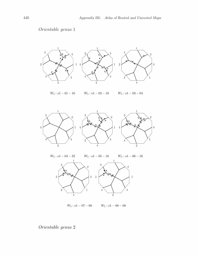
440 Appendix III Atlas of Rooted and Unrooted Maps
Orientable genus 1
2
4
1
2
1
3
3
4
YYjj KK**UU 4
2
1
2
1
3
3
4
Y *K YÆ YY I *UU1
2
3
1
4
3
2
4 Yj *W5 : o1− 01− 16 W5 : o1 − 02− 16 W5 : o1− 03− 04
4
3
1
2
1
3
2
4
4
3
1
2
1
3
4
2
YI-RKK IK66*14
3
1
2
3
1
2
4
YI-RKK IK*1W5 : o1− 04− 32 W5 : o1 − 05− 16 W5 : o1− 06− 16
1
2
3
1
4
2
3
4 YYjjKK 1
2
1
3
2
4
4
3 YYjjKKW5 : o1 − 07− 08 W5 : o1 − 08− 08
Orientable genus 2

Ax.III.4 Wheels Wn of order 6 ≥ n ≥ 4 441
1
2
1
3
4
3
2
4 i jj YIK** **1
2
1
3
4
3
2
4 Yj U U IK 1
2
1
3
2
4
3
4 YYjjjjKK YYKK UNW5 : o2− 01− 16 W5 : o2 − 02− 08 W5 : o2− 03− 16
1
2
1
3
4
2
3
4
W5 : o2 − 04− 32
Case n = 6:
Orientable genus 0
21
1
3
34
4
5
5
2 --W6 : o0 − 01− 04
Orientable genus 1

442 Appendix III Atlas of Rooted and Unrooted Maps
21
1
3
34
4
5
5
2*RRUM jj--KK 2
1
1
3
34
4
5
5
2 --UN KK RRMK jj2
1
1
3
34
4
5
5
2
W6 : o1− 01− 20 W6 : o1 − 02− 20 W6 : o1− 03− 40
21
1
3
34
4
5
5
2
21
1
3
34
4
5
5
2
--KK?i2
1
1
3
34
4
5
5
2
W6 : o1− 04− 40 W6 : o1 − 05− 20 W6 : o1− 06− 40
21
1
3
34
4
5
5
2
--K K*i2
1
1
3
34
4
5
5
2 - KK*i2
1
1
3
3
4
4
5
5
2
Yj -- *KK RRjjW6 : o1− 07− 20 W6 : o1 − 08− 20 W6 : o1− 09− 20
21
1
3
3
4
4
55
2
21
1
33
4
4
55
2
21
1
3
3
4
4
55
2
Yj KK*- RR - W6 : o1− 10− 40 W6 : o1 − 11− 40 W6 : o1− 12− 20

Ax.III.4 Wheels Wn of order 6 ≥ n ≥ 4 443
21
1
3
3
4
4
55
2
--Yj KK*RRjj2
1
1
3
3 4
4
5
5
2
--6UKKK*RRjjW6 : o1 − 13− 20 W6 : o1 − 14− 20
Orientable genus 2
21
1
3
34
4
5
5
2 --Ys KK*RR 21
1
3
34
4
5
5
2 --Yj K K*RR 21
1
3
344
5
5
2 --UKKK*RRjjW6 : o2− 01− 20 W6 : o2 − 02− 20 W6 : o3− 03− 20
21
1
3
34
4
5
5
2 - KK**i 21
1
3
34
4
5
5
2 K K 21
1
3
34
4
5
5
2
W6 : o2− 04− 20 W6 : o2 − 05− 04 W6 : o2− 06− 40

444 Appendix III Atlas of Rooted and Unrooted Maps
21
1
3
34
4
5
5
2
21
1
3
34
4
5
5
2
21
1
3
34
4
5
5
2
-- K K*iW6 : o2− 07− 40 W6 : o2 − 08− 40 W6 : o2− 09− 20
21
1
3
34
4
5
5
2 - K K*i2
1
1
3
34
4
5
5
2
21
1
3
34
4
5
5
2
W6 : o2− 10− 20 W6 : o2 − 11− 40 W6 : o2− 12− 40
21
1
3
34
4
5
5
2
21
1
3
34
4
5
5
2
21
1
3
34
4
5
5
2
W6 : o2− 13− 40 W6 : o2 − 14− 40 W6 : o2− 15− 40
21
1
3
34
4
5
5
2 -- K K* i62
1
1
3
34
4
5
5
2
21
1
3
34
4
5
5
2
- K K* iW6 : o2− 16− 20 W6 : o2 − 17− 40 W6 : o2− 18− 20

Ax.III.4 Wheels Wn of order 6 ≥ n ≥ 4 445
21
1
3
34
4
5
5
2
- K K* 6y2
1
1
3
3
4
4
5
5
2
--Yj K K**RR 21
1
3
3
4
4
55
2
W6 : o2− 19− 20 W6 : o2 − 20− 20 W6 : o2− 21− 40
21
1
3
3
4
4
5
5
2
21
1
3
3
4
4
5
5
2
21
1
3
3
4
4
55
2
W6 : o2− 22− 40 W6 : o2 − 23− 40 W6 : o2− 24− 40
21
1
3
3
4
4
55
2
21
1
3
3
4
4
55
2
21
1
33
4
4
5
5
2
--Yj K K*RRW6 : o2− 25− 40 W6 : o2 − 26− 40 W6 : o2− 27− 20
21
1
3
3
4
4
5
5
2
--Yj K K*RR 21
1
33
4
4
55
2
21
1
3
3
4
4
55
2
W6 : o2− 28− 20 W6 : o2 − 29− 40 W6 : o2− 30− 40

446 Appendix III Atlas of Rooted and Unrooted Maps
21
1
3
3
4
4
55
2
21
1
3
3
4
4
55
2
21
1
33
4
4
55
2
--Yj K K*6RRW6 : o2− 31− 40 W6 : o2 − 32− 40 W6 : o2− 33− 20
21
1
3
3
4
4
55
2
Yj K K*-- RR2
1
1
3
3 4
4
5
5
2
- K K* i 21
1
3
3 4
4
5
5
2
- K K* iW6 : o2− 34− 20 W6 : o2 − 35− 20 W6 : o2− 36− 20
21
1
3
3
4
4
5
5
2
- K K*i 2
1
1
3
3 4
4
5
5
2
--UUK MK KRRjj2
1
1
3
3
4
4
5
5
2
--Yj K K**RRW6 : o2− 37− 20 W6 : o2 − 38− 20 W6 : o2− 39− 20
21
1 3
3
4
4
5
5
2
K K 21
1
3
3 4
4
5
5
2
K KW6 : o2 − 40− 04 W6 : o2 − 41− 04

Ax.III.5 Complete graphs Kn of order 5 ≥ n ≥ 4 447
Ax.III.5 Complete graphs of order 5 ≥ n ≥ 4
Size 4: (K4 = W4, W4 is known in Ax.III.4).
Size 5:
Orientable genus 1
1
2
3IIRRRR 1
5
4
4
2
66
3
5
KKjj 1
2
3 1
5
4
4
6
23
6
5IIRR KKjjII** 1
2
3 4
1
5
2
4
66
3
5R IIIIR
K5 : o1− 01− 20 K5 : o1 − 02− 20 K5 : o1 − 03− 10
1
2
3
4
1
5
6
4
23
6
5II 1
2
3
5
1
4
4
2
66
3
5IIRRKKII ** RR
1
2
3
1
5
4
4
6
26
5
3
IIK5 : o1− 04− 02 W6 : o1 − 05− 20 W6 : o1− 06− 05
Orientable genus 2
1
2
3 1
4
5
2
4
63
5
6II 1
2
3 1
4
5
2
4
65
3
6IIRRII6 jj 1
2
3 1
4
5
2
4
66
3
5IIRRYI6
K5 : o2− 01− 04 K5 : o2 − 02− 20 K5 : o2 − 03− 20

448 Appendix III Atlas of Rooted and Unrooted Maps
1
2
3 1
4
5
2
4
66
3
5
IIRRYI6 1
2
3 1
4
5
2
6
45
6
3
1
2
3 1
4
5
2
6
46
3
5IIRRYI *-IIRR
K5 : o2− 04− 20 K5 : o2 − 05− 40 K5 : o2 − 06− 20
1
2
3 1
4
5
4
2
65
6
3
IR R 1
2
3 1
4
5
4
6
23
6
5
1
2
3 1
4
5
4
6
25
3
6IIRRII II RR
K5 : o2− 07− 05 K5 : o2 − 08− 40 K5 : o2 − 09− 20
1
2
3 1
4
5
6
2
43
6
5IIRRRR II *-RR 1
2
3 1
4
5
6
2
46
5
3
1
2
3 1
4
5
6
4
26
5
3IIRRII II*-RR?
K5 : o2− 10− 20 K5 : o2 − 11− 40 K5 : o2 − 12− 20
1
2
3 1
5
4
2
4
63
6
5IIRR K 6jjIIRR 1
2
3 1
4
5
2
4
66
3
5
1
2
3 1
5
4
2
4
66
5
3
K5 : o2− 13− 20 K5 : o2 − 14− 40 K5 : o2 − 15− 40

Ax.III.5 Complete graphs Kn of order 5 ≥ n ≥ 4 449
1
2
3 1
5
4
2
6
45
3
6
1
2
3 1
5
4
4
2
63
6
5
1
2
3 1
5
4
4
2
66
5
3IRRI K 6-j *-R
K5 : o2− 16− 40 K5 : o2 − 17− 40 K5 : o2 − 18− 20
1
2
3 1
5
4
4
6
25
3
6
1
2
3 1
5
4
4
6
2
5
3
6
1
2
3 1
5
4
4
6
2
5
3
6
IIRRKKjjII*-K5 : o2− 19− 40 K5 : o2 − 20− 40 K5 : o2 − 21− 20
1
2
3 1
5
4
4
6
2
5
3
6
1
2
3
1
4
5
2
4
65
3
6
1
2
3 4
1
5
2
6
46
3
5I IRR K 6-jIIRR
K5 : o2− 22− 40 K5 : o2 − 23− 40 K5 : o2 − 24− 20
1
2
3 4
1
5
2
6
46
3
5IIRR II 1
2
3
4
1
5
2
6
46
3
5
1
2
3
4
1
5
6
4
26
3
5IIRRRRII II*-RR
K5 : o2− 25− 10 K5 : o2 − 26− 40 K5 : o2 − 27− 20
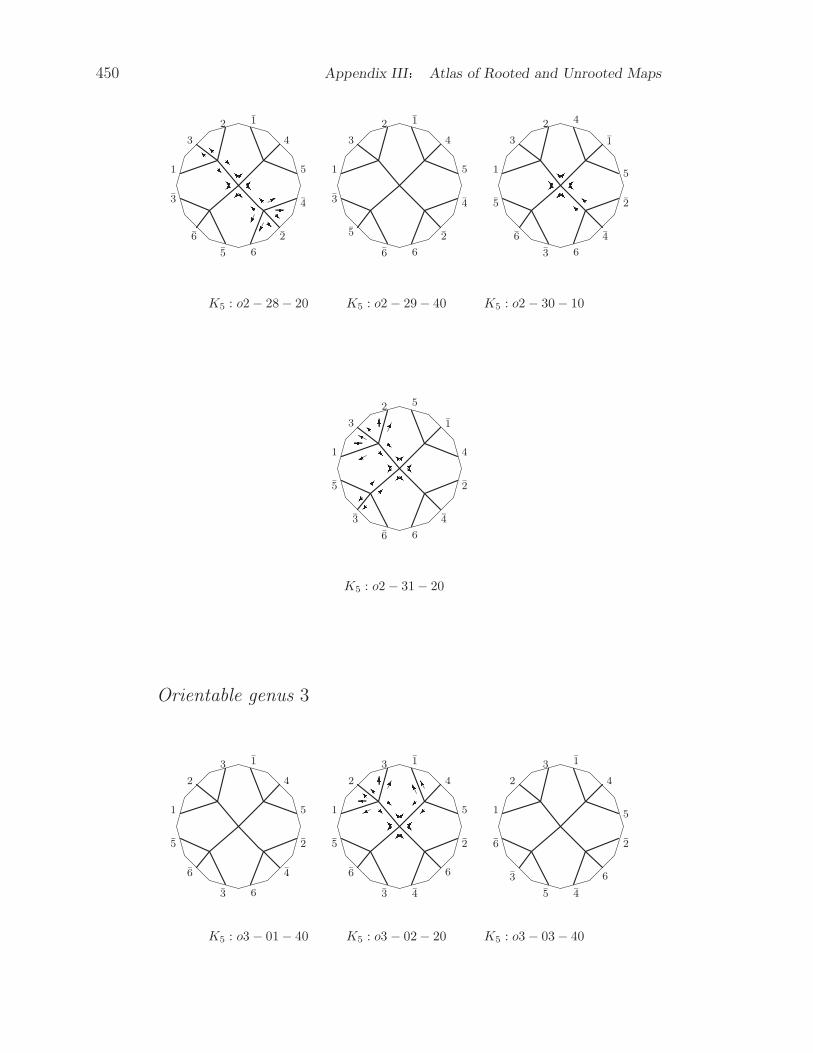
450 Appendix III Atlas of Rooted and Unrooted Maps
1
2
3
1
4
5
4
2
65
6
3
RR IIRRII II*-RR 1
2
3
1
4
5
4
2
6
5
6
3
1
2
3
4
1
5
2
4
63
6
5 IIIRRIK5 : o2− 28− 20 K5 : o2 − 29− 40 K5 : o2 − 30− 10
1
2
3
5
1
4
2
4
66
3
5
RR IIRRYI6K5 : o2− 31− 20
Orientable genus 3
1
2
3 1
4
5
2
4
63
6
5
1
2
3 1
4
5
2
4
6
3
6
5
RR IIRR II6 KK1
2
3 1
4
5
2
6
45
3
6
K5 : o3− 01− 40 K5 : o3 − 02− 20 K5 : o3 − 03− 40

Ax.III.5 Complete graphs Kn of order 5 ≥ n ≥ 4 451
1
2
3 1
4
5
2
6
4
5
3
6
1
2
3 1
4
5
2
6
45
3
6
RRIIRR66 K 6jUY 1
2
3 1
4
5
4
6
26
5
3
K5 : o3− 04− 40 K5 : o3 − 05− 20 K5 : o3 − 06− 40
1
2
3 1
5
4
2
4
65
3
6
1
2
3 1
5
4
2
6
46
5
3
RRIIRRII6UU 1
2
3 1
5
4
6
2
46
5
3
KKY IR K5 : o3− 07− 40 K5 : o3 − 08− 20 K5 : o3 − 09− 10
1
2
3 1
5
4
6
4
25
3
6
1
2
3
1
4
5
2
6
4
6
5
3
1
2
3
1
4
5
2
6
46
5
3
RR IIRRYI6 KKK5 : o3− 10− 40 K5 : o3 − 11− 40 K5 : o3 − 12− 20
1
2
3
4
1
5
2
4
65
6
3
IIRR K 6II*-RR?K5 : o3 − 13− 20

452 Appendix III Atlas of Rooted and Unrooted Maps
Ax.III.6 Triconnected cubic graphs of size in [6, 15]
Size 6: (C6,1 = K4 = W4, W4 is known above).
Size 9: (C9,2 = K3,3)
C9,1:
Orientable genus 0
43
1
1
3
2
2
4 C9,1 : o0− 01− 03
Orientable genus 1
43
1
2
3
1
2
4 UU KK 1 43
1
3
2
1
2
4 UU KK 1 **IY4
1
2
3
1
4
2 UU KK 1 **?IY3
C9,1 : o1− 01− 09 C9,1 : o1− 02− 18 C9,1 : o1− 03− 18

Ax.III.6 Triconnected cubic graphs of size in [6, 15] 453
3
4
1
3
2
1
2
4
UU 6K 1 3
4
1
1
2
3
2
4
C9,1 : o1− 04− 09 C9,1 : o1− 05− 18
Orientable genus 2
4
2
1
2
3
1
4 1UU KK 1Y11Y??IY3
4
2
1
3
2
1
4 1UU KK 1Y11Y??IY3
C9,1 : o2− 01− 18 C9,1 : o2− 02− 18
C9,2:
Orientable genus 1
1
2
3
4
1
3
2
4 6 1
2
4
3
1
3
4
2 66jj C9,2 : o1− 01− 01 C9,2 : o1− 02− 09
Orientable genus 2

454 Appendix III Atlas of Rooted and Unrooted Maps
1
2
4
3
1
3
2
4 66??* C9,2 : o2 − 01− 06
Size 12: (C12,4 is the cube)
C12,1:
Orientable genus 0
1
2
3
3
44
5
5
2
1 6???IIR- RIC12,1 : o0− 01− 12
Orientable genus 1
IIUURR ??66R- 3
2
1
3
44
5
1
2
53
2
1
3
44
5
1
2
5 -?II66RURR ??66-- - 1
2
3
3
4
4
5
1
2
5 ?KIRRRC12,1 : o1− 01− 24 C12,1 : o1− 02− 24 C12,1 : o1 − 03− 12

Ax.III.6 Triconnected cubic graphs of size in [6, 15] 455
1
2
3
3
4
4
5
2
1
5 ?KIRRR 6U?K - 2
3
1
3
44
5
5
1
23
2
1
3
44
5
5
1
2 ??IY RRRR --66? *C12,1 : o1− 04− 24 C12,1 : o1− 05− 48 C12,1 : o1 − 06− 24
2
3
1
3
44
5
5
2
13
2
1
3
44
5
5
1
2 ??IY RRRR --66? * 2
3
1
3
4
4
5
5
1
2
C12,1 : o1− 07− 48 C12,1 : o1− 08− 24 C12,1 : o1 − 09− 48
2
3
1
3
4
4
5
5
1
2 ??I RR66 --R66661
2
3
3
4
4
5
5
2
1 66???IIR- RI6 IRR **1
3
2
3
4
4
5
5
2
1
C12,1 : o1− 10− 24 C12,1 : o1− 11− 24 C12,1 : o1 − 12− 48

456 Appendix III Atlas of Rooted and Unrooted Maps
4
3
1
2
34
5
1
2
5 ??IK RU 4
3
1
2
34
5
1
2
5 ??IK RU RR II**U? ** K 4
3
1
2
34
5
1
2
5
??IK RU C12,1 : o1− 13− 12 C12,1 : o1− 14− 24 C12,1 : o1 − 15− 12
Orientable genus 2
3
2
1
3
44
5
1
2
5
1
2
3
2
1
3
44
5
5
1
2
4
3
3
2
1
4
5
5
C12,1 : o2− 01− 28 C12,1 : o2− 02− 48 C12,1 : o2 − 03− 48
1
2
4
3
2
3
1
4
5
5
1
2 4
3
3
2
1
4
5
5
1
2 4
3
3
2
1
4
5
5 ?IY6R? **RjK 6C12,1 : o2− 04− 48 C12,1 : o2− 05− 48 C12,1 : o2 − 06− 24

Ax.III.6 Triconnected cubic graphs of size in [6, 15] 457
1
2
4
3
3
2
1
4
5
5 ?IYUU R K **RjK 6 1
2
4
3
3
2
1
4
5
5
1
2 4
3
3
2
1
4
5
5
C12,1 : o2− 07− 24 C12,1 : o2− 08− 24 C12,1 : o2 − 09− 48
1
2 4
3
3
2
1
4
5
52
3
1
3
4
4
5
5
1
2
1
2
3
3
4
4
5
5
2
1
C12,1 : o2− 10− 48 C12,1 : o2− 11− 48 C12,1 : o2 − 12− 48
1
2
4
3
3
2
1
4
5
5 ?IY6R?RR U?RRKK1
2
4
3
3
2
1
4
5
5
1
2
4
3
3
2
1
4
5
5
C12,1 : o2− 13− 24 C12,1 : o2− 14− 48 C12,1 : o2 − 15− 48
1
2
4
3
3
2
1
4
5
5
1
2
4
3
3
2
1
4
5
5
1
2 4
3
3
2
1
4
5
5
C12,1 : o2− 16− 48 C12,1 : o2− 17− 48 C12,1 : o2 − 18− 48

458 Appendix III Atlas of Rooted and Unrooted Maps
1
2
4
3
3
2
1
4
5
5 IYURU U?jRKI K66 1
2
4
3
3
2
1
4
5
5
1
2
4
3
3
2
1
4
5
5 IYURU **jRKI K66C12,1 : o2− 19− 24 C12,1 : o2− 20− 48 C12,1 : o2 − 21− 24
1
2 4
3
3
2
1
4
5
5 IYURU U *jRKI *6 3
2
1
3
45
4
5
2
1
32
1
3
45
4
5
2
1 RU6RR ?U--66C12,1 : o2− 22− 24 C12,1 : o2− 23− 48 C12,1 : o2 − 24− 24
3
2
1
3
45
4
5
2
1
13
2
1
3
45
4
5
2 **? U6 U?RU--66 I**3
4
1
3
25
4
1
2
5 KK 66UU--RRKK ?II
C12,1 : o2− 25− 48 C12,1 : o2− 26− 24 C12,1 : o2 − 27− 24
3
4
1
3
25
4
1
2
5 KK 66UU--RRKK RR6
C12,1 : o2− 28− 24
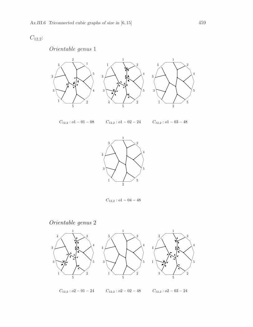
Ax.III.6 Triconnected cubic graphs of size in [6, 15] 459
C12,2:
Orientable genus 1
21
5
4
25
1
3
3
4 6?II1
2
4
5
25
4
3
3
1 66??I66RRR ???I6-R6?I1
2
4
5
52
1
3
3
4
C12,2 : o1− 01− 08 C12,2 : o1− 02− 24 C12,2 : o1 − 03− 48
1
2
4
5
52
1
3
4
3
C12,2 : o1− 04− 48
Orientable genus 2
1
2
4
5
25
1
3
3
4 6??R 66RR???I6-RI1
2
4
5
25
1
3
4
3
1
2
4
5
25
3
1
4
3 6??- 66RR???I6RR6?IC12,2 : o2− 01− 24 C12,2 : o2− 02− 48 C12,2 : o2 − 03− 24

460 Appendix III Atlas of Rooted and Unrooted Maps
1
2
5
4
25
3
1
3
4 66R?II??66RR-RII ??I61
2
4
5
52
1
3
4
3 12
4
5
521
3
4
3 6??II??66RR-RI6 IIR?RC12,2 : o2− 04− 24 C12,2 : o2− 05− 48 C12,2 : o2 − 06− 24
1
2
4
5
5
2
1
3
4
3 66??YR 66RR? ??RR-6?YY
1
2
4
5
52
1
3
4
3 6?Yj?1
2
4
5
52
1
3
4
3
C12,2 : o2− 07− 24 C12,2 : o2− 08− 08 C12,2 : o2 − 09− 48
1
2
4
5
52
1
3
4
3 1
2
4
5
52
1
3
4
3 6?I??RRI6661
2
4
5
52
1
3
4
3
C12,2 : o2− 10− 48 C12,2 : o2− 11− 16 C12,2 : o2 − 12− 48
C12,3:
Orientable genus 1

Ax.III.6 Triconnected cubic graphs of size in [6, 15] 461
1
2
4
3
3
1
5
4
2
5 66I RRR YY 1
2
4
3
3
1
5
4
2
5 66I?RR?IRR 66IY---??
1
2
4
3
3
1
5
4
2
5 66II RR??66RR ??IIIKC12,3 : o1− 01− 12 C12,3 : o1− 02− 24 C12,3 : o1 − 03− 24
1
2
4
3
3
1
5
4
2
5 ??II66RR1
2
4
33
1 5
4
2
5 ??66IRRIC12,3 : o1 − 04− 12 C12,3 : o1− 05− 12
Orientable genus 2
1
2
4
3
3
1
5
4
2
5 66II RRRR ??66---
II RR 1
2
4
3
3
15
4
2
5 I 1
2
4
3
3
1
5
4
2
5 I??I66RRRR --II II--
C12,3 : o2− 01− 24 C12,3 : o2− 02− 03 C12,3 : o2 − 03− 24

462 Appendix III Atlas of Rooted and Unrooted Maps
1
2
4
3
3
1
5
4
2
5 66I RRR YY??I66RR R 1
2
4
3
3
1
5
4
2
5 1
2
4
3
3
1
5
4
2
5 66I RRR YYR II?? -- RC12,3 : o2− 04− 24 C12,3 : o2− 05− 48 C12,3 : o2 − 06− 24
1
2
4
3
3
1
5
4
2
5 1
2
4
3
3
1
5
4
2
5 66I RRR YYR RII-- ?? 1
2
4
3
3
1
5
4
2
5 66I RRR YYR? ?6U6I-- RC12,3 : o2− 07− 48 C12,3 : o2− 08− 24 C12,3 : o2 − 09− 24
1
2
4
3
3
1
5
4
2
5 I??I 1
2
4
33
1
5
4
2
5 66I RR??I66RR ??I6-- 1
2
4
33
1 5
4
2
5 66I RRR YY??I66RR-- RC12,3 : o2− 10− 06 C12,3 : o2− 11− 24 C12,3 : o2 − 12− 24

Ax.III.6 Triconnected cubic graphs of size in [6, 15] 463
1
2
4
3
3
1
5
4
2
5 IC12,3 : o2− 13− 03
C12,4:
Orientable genus 0
2
4
4
5
1
15
3
3
2 C12,4 : o0− 01− 01
Orientable genus 11
5
4
4
2
1
5
3
3
2 j?? 1
5
4
4
2
1
5
3
3
2 j IIRI 66RR??* 1
5
4
4
2
1
5
3
3
2 jRIC12,4 : o1− 01− 03 C12,4 : o1− 02− 12 C12,4 : o1 − 03− 03

464 Appendix III Atlas of Rooted and Unrooted Maps
1
5
4
4
2
1
5
3
3
2 j I66??* 1
5
4
4
21
5
3
3
2 jC12,4 : o1 − 04− 08 C12,4 : o1− 05− 01
Orientable genus 2
1
5
4
4
21
5
3
3
2 jIR j 1
5
4
4
21
5
3
3
2 jIR jR I II??66?? K 6R ?66 6 1
5
4
4
21
5
3
3
2 jIjI??66?? K 6C12,4 : o2− 01− 04 C12,4 : o2− 02− 24 C12,4 : o2 − 03− 12
1
5
4
4
2
1
5
3
3
2 j 66j 1
54
4
2
1
5
3
3
2 j IIjIR R I??--
1
5
4
4
2
1
5
3
3
2 j 66j IIRRIR ?? ??IIII
C12,4 : o2− 04− 04 C12,4 : o2− 05− 12 C12,4 : o2 − 06− 24
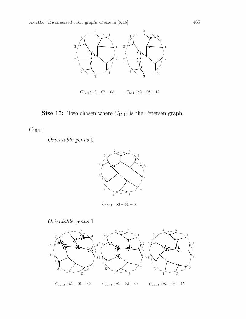
Ax.III.6 Triconnected cubic graphs of size in [6, 15] 465
1
54
4
21
5
3
3
2 jI??66?6 1
5
4
4
21
5
3
3
2 j??66?? --66-
C12,4 : o2 − 07− 08 C12,4 : o2− 08− 12
Size 15: Two chosen where C15,14 is the Petersen graph.
C15,11:
Orientable genus 0
2 4
4
5
1
1
56
6
3
3
2 *IC15,11 : o0 − 01− 03
Orientable genus 1
1
2
5
4
4
1
6
5
3
6
3
2 I-I-R? I6--RR RR?? R ? Y-- II 4 5
1
2
4
1
56
6
3
3
2 --??II -66RRRjII 66 4 5
1
4
2
6
51
6
3
3
2 -- IY 66--??IC15,11 : o1− 01− 30 C15,11 : o1 − 02− 30 C15,11 : o2− 03− 15

466 Appendix III Atlas of Rooted and Unrooted Maps
4 5
1
4
2
6 5
16
3
3
2 -- IY -jj 4
51
4
2
6
51
6
3
3
2 I-- IIY RR ---C15,11 : o1 − 04− 15 C15,11 : o1− 05− 15
Orientable genus 2
4 5
1
2
4
1
56
6
3
3
2
45
1
2
4
1
5 6
6
3
3
2 --??II -66RRRR ???? ---I6 --4 5
1
2
4
1
56
6
3
3
2
C15,11 : o2− 01− 60 C15,11 : o2 − 02− 30 C15,11 : o2− 03− 60
45
1
2
4
1
56
6
3
3
2 --??II -66RRRR ???? ---I6 --4
5
1
4
2
6
5
1
6
3
3
2 I-- IIY RR --- 4
5
1
4
2
6
51
6
3
3
2 I-- IIY RR ----RR? IIII--??C15,11 : o2− 04− 30 C15,11 : o2 − 05− 15 C15,11 : o2− 06− 30
4
51
4
2
6
51
6
3
3
2
4
5
1
4
2
6
51
6
3
3
2 I-- IIY RR --- RR ?R??II 66 4
51
4
2
6
5
1
6
3
3
2 -- II II--RRRR ?RII RRII--C15,11 : o2− 07− 60 C15,11 : o2 − 08− 30 C15,11 : o2− 09− 30

Ax.III.6 Triconnected cubic graphs of size in [6, 15] 467
4
51
4
2
65
1
6
3
3
2 -- II II-- --?RR ?R?6 64
51
4
2
6 5
16
3
3
2 -- II II-- -?RR? -RRI I I 4 5
1
4
2
6
5
1
6
3
3
2 -- II 66-66RRRR ?RII -??Y IjC15,11 : o2− 10− 30 C15,11 : o2 − 11− 30 C15,11 : o2− 12− 30
4 5
1
4
2
6
51
6
3
3
2
4 5
1
4
2
6 5
1
6
3
3
2 -- II 66--jj ? ?II--YY--
45
1
4
2
6
51
6
3
3
2 --II 66--RRII R??? IR**66 YYC15,11 : o2− 13− 60 C15,11 : o2 − 14− 30 C15,11 : o2− 15− 30
4
5
1
4
2
65
1
6
3
3
2 *Y 45
1
4
2
6
5
1
6
3
3
2
4 5
1
4
2
6
51
6
3
3
2 -- YI 66--RR? ??II--IIjjC15,11 : o2− 16− 03 C15,11 : o2 − 17− 60 C15,11 : o2− 18− 30
45
1
4
2
6
51
6
3
3
2 -- IY 66--jj RR?? ?? -j 66I 4 5
1
4
2
6
51
6
3
3
2 -- IY 66--jj RR?? ?? Ij 66 45
1
4
2
6 5
1
6
3
3
2 -- II - jj II-- 66??666C15,11 : o2− 19− 30 C15,11 : o2 − 20− 30 C15,11 : o2− 21− 30

468 Appendix III Atlas of Rooted and Unrooted Maps
4 5
1
4
2
6 5
16
3
3
2 -- II 66--jj ? ?II--YY--
45
1
4
2
65
1
6
3
3
2 -- II -jj YY4 5
1
4
2
6 5
1
6
3
3
2
C15,11 : o2− 22− 30 C15,11 : o2 − 23− 15 C15,11 : o2− 24− 60
45
1
4
2
6
5
1
6
3
3
2 -- IY 66--RR-R 66II ??II-- 4 5
1
4
2
6
51
6
3
3
2 -- II 66--RR ??I--II-R?45
1
4
2
6
5
1
6
3
3
2 -- IY 66--??YC15,11 : o2− 25− 30 C15,11 : o2 − 26− 30 C15,11 : o2− 27− 15
4 5
1
4
2
6
5
1
6
3
3
2 -- YI 66-- 66?? ??Y YIR ??C15,11 : o2 − 28− 30
Orientable genus 3
45
1
4
2
6
51
6
3
3
2
45
1
4
2
6
51
6
3
3
2
4 5
1
4
2
6
5
1
6
3
3
2
C15,11 : o3− 01− 60 C15,11 : o3 − 02− 60 C15,11 : o3− 03− 60
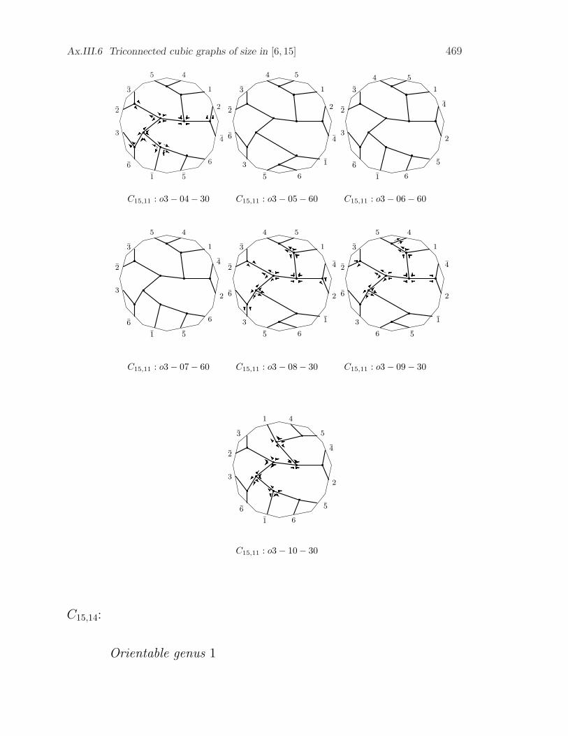
Ax.III.6 Triconnected cubic graphs of size in [6, 15] 469
45
1
4
2
6
51
6
3
3
2 -- YI 66--RRRR 66II YIjj ?4 5
1
4
2
65
1
6
3
3
2
4 5
1
4
2
6
5
1
6
3
3
2
C15,11 : o3− 04− 30 C15,11 : o3 − 05− 60 C15,11 : o3− 06− 60
45
1
4
2
6
51
6
3
3
2
4 5
1
4
2
65
1
6
3
3
2 -- YY 66--jj ??YY--RR ?R??45
1
4
2
6 5
1
6
3
3
2 -- YY 66--jj ??YY-- **C15,11 : o3− 07− 60 C15,11 : o3 − 08− 30 C15,11 : o3− 09− 30
4
5
1
4
2
6
5
1
6
3
3
2 -- II II--RR IIRR--II-R?C15,11 : o3 − 10− 30
C15,14:
Orientable genus 1

470 Appendix III Atlas of Rooted and Unrooted Maps
1
2
5 4
1
3
5
6
62
4
3
--I6RIC15,14 : o1 − 01− 10
Orientable genus 2
1
2
54
1
3
5
6
6 2
4
3
--I6?R 66 R?R ??I I- 1
2
54
1
3
5
6
6 2
4
3
--I6R?6666??--66 6?1
2
54
1
3
5
6
6 2
4
3
--I6?R- RR6?R 6jjC15,14 : o2− 01− 30 C15,14 : o2 − 02− 30 C15,14 : o2− 03− 30
1
2
5 4
1
3
5
6
62
4
3
--I6?R666??--6??III6 1
2
54
1
3
5
6
62
4
3
--I666R ?66 ???--I6 61
2
5 4
1
3
5
6
62
4
3
--I6RIC15,14 : o2− 04− 20 C15,14 : o2 − 05− 30 C15,14 : o2− 06− 10

Ax.III.6 Triconnected cubic graphs of size in [6, 15] 471
1
2
54
1
3
5
6
62
4
3
--RIC15,14 : o2 − 07− 06
Orientable genus 3
1
2
54
1
3
5
6
6 2
4
3
1
2
54
1
3
5
6
62
4
3
--I6?R66RR6C15,14 : o3 − 01− 60 C15,14 : o3− 02− 20

Bibliography
Baxter, R.J.
[Bax1] Dichromatic polynomials and Potts models summed over rooted
maps, Annals Combin. 9 (2001), 17–36.
Bender, E.A., Z.C. Gao, L.B. Richmond and N.C. Wormald
[BeG1] Asymptotic properties of rooted 3-connected maps on surfaces,
J. Austral. Math. Soc., A60 (1996), 31–41.
Birkhoff, G.D.
[Bir1] The reducibility of maps, Amer, J. Math. 35 (1913), 115– 128.
Cai, J.L. and Y.P. Liu
[CaL1] The number of rooted nearly cubic c-nets, Acta Math. Appl.
Sinica, 17(2001), 29–37.
[CaL2] The enumeration of rooted nonseparable nearly cubic maps, Dis-
crete Math., 207 (1999), 9–24.
Chai, Z. and Y.P. Liu
[CiL1] Up-embeddability of a graph with maximum face degree 6(in Chi-
nese with English abstract), J. Beijing Jiaotong Univ., 26(2005),
6:94-97.
Chen, Y.C. and Y.P. Liu
[CnL1] Maximum genus, girth and maximum non-adjacent edge set, Ars
Combin., 79(2006), 145–159.
Chen, Y.C., Y.P. Liu and R.X. Hao
[CnR1] Structure for a graph with average genus, J. Appl. Math.& Com-
put., 21(2006), 45–55.
Dehn, M.
[Deh2] Uber Kombinatoriche Topologie, Acta Math., 67 (1936), 123–

Bibliography 473
168.
Dixon, J.M. and B. Mortimer
[DiM1] Permutation Groups, Springer, 1996.
Dong, G.H. and Y.P. Liu
[DoL1] Results of the maximum genus of graphs, Science in China, A50
(2007), 1563–1570.
Edmonds, J.R.
[Edm1] A combinatorial representation for polyhedral surfaces, Notices
Amer. Math. Soc., 7 (1960), 646.
Garey, M. R. and D. S. Johnson
[GaJ1] Computers and Intractability, W. H. Freeman, 1979.
Gauss, C. F.
[Gau1] Werke (Teubner, Leipzig, 1900), 272, 282– 286.
Hao, R.X., Cai J.L. and Liu Y.P.
[HaC1] Enumeration of maps on the projective plane[J] Acta Math. Appl.
Sinica, English Series 17(2001), 567–573.
Hao, R.X. and Y.P. Liu
[HaL1] On chromatic polynomials of some kinds of graphs, Acta Math.
Appl. Sinica, Eng.Series 20(2004), 239–246.
He, W.L. and Y.P. Liu
[HeL1] A note on the maximum genus of graph G3, J. Systems Science
and Information, 1(2003), 615–619.
Heffter, L.
[Hef1] Ueber das Problem der Nachbargebiete, Math. Ann., 38 (1891),
477–508.
Hilbert, D. and S. Cohn-Vossen
[HiC1] Anschauliche Geometrie, Julius Springer, 1932.
Huang, Y.Q. and Y.P. Liu
[HuL1] Face size and the maximum genus of a graph, J. Combin. Theory,

474 Bibliography
B80(2000), 356–370.
H.Iseri
[Ise1] Smarandache manifolds, American Research Press, Rehoboth,
NM,2002.
Kempe, A. B.
[Ke1] On the geographical problem of the four colours, Amer. J. Math.
2 (1879), 193– 200.
Kwak, J. H. and J. Lee
[KwL1] Enumeration of graph coverings and surface branched coverings,
Combinatorial and Computational Mathematics: Present and Fu-
ture,Edited by Hong et al, World Scientific, 2001, 97–161.
[KwL2] Genus polynomials of dipoles, Kyungpook Math. J. 33 (1993),
115–125.
Li, D.M. and Y.P. Liu
[LiL1] Maximum genus, girth and connectivity, Europ. J. Combin.,
21(2000), 651–657.
Li, L.F. and Y.P. Liu
[LiP1] The genus distribution of a type of cubic graphs (in Chinese with
English abstract), J. Beijing Jiaotong Univ., 28(2005), 39–42.
Li, Z.X. and Y.P. Liu
[LiQ1] Chromatic sums of rooted triangulations on the projective plane,
J. Appl. Math.&Comput., 18(2005), 183–196.
[LzL2] Chromatic sums of 2-edge connected maps on the plane, Discrete
Math., 296(2005), 211–223.
Little, C. H. C.
[Lit1] Cubic combinatorial maps, J. Comb. Theory, B44 (1988), 44–63.
Liu, Y.P.
[Liu1] The nonorientable maximum genus of a graph(in Chinese with
English Abstract), Sientia Sinica, Special Issue on Math. I
(1979), 191– 201.
Bibliography 475
[Liu2] The orientable maximum genus of a graph, Scientia Sinica, Spe-
cial Issue on Math. II(1979), 41– 55.
[Liu3] A note on the Edmonds surface dual theorem(in Chinese with
Englias Abstract), OR Transactions, 2:1 (1983), 62–63.
[Liu4] A polyhedral theory on graphs, Acta Math. Sinica 10(1994),
136–142.
[Liu5] Theory of Graphic Embeddability(in Chinese), Science Press, Bei-
jing, 1994.
[Liu6] Embeddability in Graphs, Kluwer, Boston, 1995.
[Liu7] Combinatorial invariants on graphs, Acta Math. Sinica, 11 (1995),
211–220.
[Liu8] Enumerative Theory of Maps. Kluwer, Boston, 1999.
[Liu9] Theory of Counting Combinatorial Maps(in Chinese), Science
Press, Beijing, 2001.
[Liu10] Introduction to Combinatorial Maps, POSTECH, Pohang, 2002.
[Liu11] Map color theorem and surface embedding of graphs(I–V)(in Chi-
nese), Math. Theory and Prac., No.1(1981), 65–78; No.2(1981),59–
63; No.3(1981), 33–44; No.4(1981), 33–41; No.1(1982), 34–44.
[Liu12] New approaches to the double cover conjecture of graphs by cir-
cuits, OR Transactions, 4(2000), 50–54.
[Liu13] Advances in Combinatorial Maps(in Chinese), Northern Jiaotong
Univ. Press, Beijing, 2003.
[Liu14] Algebraic Principles of Maps(in Chinese), Higher Education Press,
Beijing, 2006.
[Liu15] Theory of Polyhedra, Science Press, Beijing, 2008.
[Liu16] A new method for counting rooted trees with vertex partition,
Sciences in China, A51(2008), 2000–2004.
[Liu17] Theory of Counting Combinatorial Maps(2nd and extended Ed.,
in Chinese), Science Press, Beijing, 2008.
[Liu18] Topological theory on Graphs, USTC Press, Hefei, 2008.
[Liu19] General Theory of Map Census, Sience Press, Beijing, 2009.

476 Bibliography
[Liu20] Theory of Graphic Embeddability(2nd and extended Ed., in Chi-
nese), Science Press, Beijing, 2010.
Liu, Yi. and Y.P. Liu
[LpL1] A characterization of the embeddability of graphs on the surface
of given genus, Chin. Ann. Math., 17B(1996), 457–462.
Liu, W.Z. and Y.P. Liu
[LwL1] Enumeration of three kinds of rooted maps on the Klein bottle,
J. Appl. Math. Comput., 24(2007), 411–419.
[LwL2] 5-essential rooted maps on N5, Utiliyas Math., 72(2007), 51–64.
MacLane, S.
[Mac1] A structural characterization of planar combinatorial graphs,
Duke Math. J., 3(1937), 416–472.
Mao, L.F.
[Mao1] Automorphism Groups of Maps, Surfaces and Smarandache Ge-
ometries, American Research Press, 2005.
[Mao2] A new view of combinatorial maps by Smarandache’s notion, in
Selected papers on Mathematical Combinatorics(I), 49-74, World
Academic Union, 2006.
[Mao3] Smarandache Multi-Space Theory, Hexis, Phoenix,American 2006.
[Mao4] Combinatorial Geometry with Applications to Field Theory, In-
foQuest, 2009.
[Mao5] Combinatorial speculation and combinatorial conjecture for math-
ematics, International J.Math. Combin. Vol.1(2007), No.1, 1-19.
Mao, L.F. and Y.P. Liu
[MaL1] A new approach for enumerating maps on orientable surfaces,
Austral. J. Combin., 30(2004), 247–259.
Mao, L.F., Y.P. Liu and F. Tian
[MaT1] Automorphisms of maps with a given underlying graph and their
application to enumeration, Acta Math. Sinica, 21(2005), 225–
236.

Bibliography 477
Mao, L.F., Y.P. Liu and E.L. Wei
[MaW1] The semi-arc automorphism group of a graph with application
to map enumeration, Graphs and Combin., 22(2006), 83–101.
Massey, W.
[Mss1] Algebraic Topology, Harcourt, 1967.
Mullin, R.C. and P.J. Scellenberg
[MuS1] The enumeration of c-nets via quadrangulations, J. Combin.
Theory, 4(1963), 259–276.
Ore, O.
[Ore1] The Four Color Problem, Acad. Press, 1967.
Ren, H. and Y.P. Liu
[ReL1] 4-regular maps on the Klein bottle, J. Combin. Theory, B82
(2001), 118–137.
[ReL2] Enumerating near 4-regular maps on the sphere and the torus,
Discrete Appl. Math., 110 (2001), 273–288.
[ReL3] Bisingular maps on the sphere and the projective plane, Discrete
Math., 223 (2000), 275–285.
Ringel, G.
[Rin1] The toroidal thickness of complete graphs (in German), Math.
Z., 87 (1985), 14– 26.
[Rin2] Farbungsprobleme auf Flachen und Graphen, VEB Deutscher Ver-
lag der Wis-senschafteng, 1959.
[Rin3] Map Color Theorem, Springer, 1974.
Shao, Z.L. and Y.P. Liu
[ShL1] Genera of repeated edge amalgamation for two types of graphs(in
Chinese), J. Beijing Jaotong Univ., 31(2007), 3: 58–60.
F.Smarandache
[Sma1] A Unifying Field in Logics. Neutrosopy: Neturosophic Probabil-
ity, Set, and Logic, American research Press, Rehoboth, 1999.
[Sma2] Mixed noneuclidean geometries, eprint arXiv: math/0010119,
10/2000.

478 Bibliography
F.Smarandache, V.Christianto, Y.H.Fu, et.al
[SCF1] Unfolding the Labyrinth: Open Problems in Physics, Mathemat-
ics, Astrophysics and Other Areas of Science, Hexis, Phoenix,
2006.
Stahl, S.
[Sta1] Generalized embedding schemes, J. Graph Theory, 2 (1978), 41–
52.
[Sta2] A combinatorial analog of the Jordan curve theorem, J. Comb.
Theory, B35 (1983), 1– 21.
Tutte, W. T.
[Tut1] Combinatorial oriented maps, Canad. J. Math., 31(1979), 986–
1004.
[Tut2] On the spanning trees of self-dual maps, Ann. New York Acad.
Sci., 319 (1970), 540–548.
[Tut3] Graph Theory, Addison–Wesley, 1984.
Vince, A.
[Vin1] Combinatorial maps, J. Comb. Theory 34, (1983), 1–21.
[Vin2] Map duality and generalizations, Ars Combin., 39 (1995), 211–
229.
Wan, L.X. and Y.P. Liu
[WaL1] The orientable genus distribution of a new type of graphs (in Chi-
nese with English abstract), J. Beijing Jiaotong Univ., 26(2005),
65-68.
[WaL2] Orientable embedding distributions by genus for certain type of
non-planar graphs, Ars Combin., 79(2006), 97–105.
Wang, H.Y. and Y.P. Liu
[WgL1] Maximum genus of a 2-connected graph with diameter 3(in Chi-
nese with English abstract), J. Xinyang Teacher College(NS),
17(2004), 381–384.
Wei, E.L. and Y.P. Liu
[WiL1] Strong maximum genus of a type of graphs, J. Northern Jiaotong

Bibliography 479
Univ., 26(2002), 19–21.
[WeL2] Weak embedding of planar graphs, J. Appl. Math.& Comput.,
21(2006), 175–187.
Xu, Y. and Y.P. Liu
[XuL1] The number of pan-fan maps on the projective plane, Utilitas
Math., 72(2007), 279–286.
[XuL2] Counting pan-fan maps on nonorientable surfaces, Ars Combin.,
83(2007), 15–32.
Yang, Y. and Y.P. Liu
[YaL1] Total genus distribution of two classes of 4-regular graphs, Acta
Math. Sinica(CS), 50(2007), 1191–1200.
[YaL2] Flexibility of embeddings of bouquets of circles on the projective
plane and Klein bottle, Electron. J. Combin., 14(2007), #R80,
1–12.
Zha, S.Y.
[Zha1] On minimum-genus embedding, Discrete Math., 149(1996), 261–
278.
Zhao, X.M. and Y.P. Liu
[ZhL1] On the problem of genus polynomials of tree-like graphs (in Chi-
nese with English abstract), J. Beijing Jiaotong Univ., 28(2004),
7–11.
[ZhL1] Unimodality of genus distribution for tree graphs(in Chinese), J.
Shanxi Univ.(NS), 29(2006), 242–244.
Zhu, Z.L. and Y.P. Liu
[ZuL1] The genus distributions of two types of graphs (in Chinese with
English abstract), J. Shenyang Normal Univ.(NS), 24(2006), 1–
5.
Terminology
(i, j)-edge, 186
(i, j)-map, 58
(i, j)f-map, 123
(i∗, j∗)-map, 58
(l, s)∗-edge, 186
(x, y)-difference, 348
〈x, y〉-difference, 348
1-addition, 244
1-product, 244
C∗-oriented planarity, 309
H-valency, 209
i-connected, 35
i-cut, 35
i-map, 57
i-section, 301
i-vertex, 194
j-face, 194
j∗-map, 58
n-cube, 141
N -standard map, 149
O-standard map, 126
s-manifold, 29
V -code, 298
1-set, 375
1st level segment, 285
2-partition, 34, 122
3-map, 123
absolute genus, 158
absolute norm, 307
admissible, 284
appending an edge, 86
arc, 2
articulate vertex, 187, 262
articulation, 303
assignment, 283
associate net, 121
associate surface, 283
associate surface graph, 288
automorphism, 190, 331
automorphism group, 192, 331
balanced, 121
barfly, 146
Base map, 317
base map, 262
basic adding, 96
basic appending, 96
basic contracting, 96
basic contracting irreducible, 101
basic deleting, 96
basic deleting edge irreducible, 101
basic equivalence, 112
basic partition, 45
basic permutation, 43
basic set, 41
basic splitting, 96
basic subtracting, 96
basic subtracting irreducible, 102
basic transformation, 96
Betti number, 17
bi-matching map, 208
bi-pole map, 232
biboundary, 310
480

Terminology 481
bijection, 42, 101
bipartite, 100
bipartite graph, 6
bipole, 37
Blissard operator, 346
boundary identification, 306
boundary identifier, 306
bouquet, 37, 213
branch, 287
butterfly, 125
cavity, 209
cellular embedding, 381
celluliform, 300
chromatic number, 40
circuit, 5
circuit partition, 7
class of basic equivalence, 113
co-order, 113
cocircuit oriented map, 309
cocircuit oriented planarity, 309
cocircular map, 309
cocirculation, 310
cocycle, 34, 122
commutative, 168
completely symmetrical, 197
composition, 4
conjugate axiom, 46
conjugate), 46
connected, 5
contractible, 10
contractible point, 300
contracting, 76
contraction, 300
coorder, 19, 169
corank, 17
cosemiedge, 56
crosscap polynomial, 289
crosscap, 13
crossing number, 40
cubic, 209
cut-vertex, 59
cuttable, 68, 69
cutting, 68
cutting face, 69
cutting graph, 69
cutting vertex, 68
cycle, 43
cyclic number, 17
cyclic permutation, 43
decomposition, 37
decreasing duplition, 112
decreasing subdivision, 112
degree, 7
deleting, 72
different indices, 19
different signs, 187
digraph, 5
dipole, 341
directed pregraph, 2
distinct, 283
distinct, 376
double edge, 70
double H-map, 210
double leaf, 308
double link, 70
double loop, 70
double side curve), 10
down-embeddable, 20

482 Terminology
dual, 49, 65, 377
dual Eulerian map), 100
dual H-map, 210
dual map, 66
dual matching, 208
dual matching map, 208
dual regular, 57
dual trail code, 179
edge, 2
edge independent partition), 59
edge rooted, 202
edge-automorphism, 330
edge-isomorphism, 329
efficient, 176
elementary equivalence, 378
elementary transformation, 377
embedding, 381
embedding), 17
empty pregraph, 2
end segment, 286
end, 1, 56
enumerating function, 241
equilibrious embedding, 64
equilibrium, 64
equivalent class, 113
Euler characteristic, 20
Euler characteristic(Euler charac-
teristic), 113
Euler graph, 7
Eulerian, 361
Eulerian characteristic, 377
even, 361
even assigned conjecture, 102
even assigned map, 100
even pregraph, 7
eves-cyclic, 231
exchanger, 287
expanded tree, 283
expansion, 383
face, 17, 49, 377
face regular, 57
face representative, 121
face rooted, 202
face-algorithm, 172
face-regular, 195
fan-flower, 317
father, 286
favorable embedding, 60
favorable map, 60
favorable segment, 301
feasible segment, 300
feasible sequence, 298
finite pregraph), 2
finite recursion principle), 6
finite restrict recursion principle,
6
first operation, 47
first parameter, 349
fixed point, 191
flag, 384
full cavity, 209
general, 350
generalized Halin graph, 38
generated group, 50
genus polynomial, 289
genus, 138
graph, 5

Terminology 483
ground set, 2, 42
Halin graph, 307
Halin map, 262
Hamilton map, 123
Hamiltonian circuit, 122
Hamiltonian graph, 122
handle polynomial, 289
handle, 13
harmonic link, 70
harmonic loop, 70
hexagonalization), 102
homotopic), 10
identity, 192
immersion, 33
incidence equation, 34
incident pair, 100
included angle, 56
increasing duplition, 112
increasing subdivision, 112
independent face set, 209
independent pair, 100
independent set, 100
induced, 44, 99
infinite pregraph, 2
initial end, 2
inner rooted, 311
inner vertex, 262
interlaced, 134
interpolation theorem, 21
irreducible, 140, 299
isomorphic, 385
isomorphic class, 168
isomorphism, 165, 330
joint sequence, 187
joint tree, 18, 187
Klein group, 22
Klein model, 31
ladder, 293
left projection, 346
link, 70
link bundle, 37, 403
link map, 194
loop, 70
loop bundle, 37
loop map, 67
loopless map, 265
map, 50
map geometry, 29
maximum genus, 21
maximum genus embedding, 162
maximum nonorientable face num-
ber embedding, 63
maximum nonorientable genus, 162
maximum orientable face number
embedding, 63
meson functional, 346
minimum genus, 21
minimum genus embedding, 162
minimum nonorientable genus, 162
minimum nonorientable genus em-
bedding, 63
minimum orientable genus embed-
ding, 63
multiplicity, 333
near quadrangulation, 261

484 Terminology
near regular, 266
near triangulation, 261
necklace, 293
network, 6
node, 2
noncuttable, 68, 69
noncuttable block, 69
nonorientable form, 290
nonorientable, 10, 104, 374
nonorientable favorable genus, 162
nonorientable genus, 11, 158, 162
nonorientable pan-tour conjecture,
163
nonorientable pan-tour genus, 162
nonorientable pan-tour maximum
genus, 162
nonorientable preproper genus, 162
nonorientable proper map conjec-
ture, 163
nonorientable rule, 153
nonorientable rule 3, 155
nonorientable single peak conjec-
ture, 39
nonorientable small face proper map
conjecture, 163
nonorientable tour genus, 162
nonorientable tour map conjecture,
163
nonorientable tour maximum genus,
162
nonseparable, 58
odd circuit, 34
orbit, 23, 43
order, 19, 40, 43, 169, 192
orientable genus polynomial, 389
orientable, 10, 104, 374
orientable genus, 11, 138
orientable minimum pan-tour genus,
142
orientable pan-tour conjecture, 142
orientable pan-tour maximum genus,
143
orientable proper map conjecture,
142
orientable single peak conjecture,
39
orientable tour conjecture, 142
pan-Halin map, 262
pan-tour face), 142
pan-tour map, 142
parallel, 134
partition, 2
path, 5
petal bundle, 125, 213
planar graph, 35
planar map, 141
planar pedal bundle, 217
plane tree, 297
planted tree, 263, 297
point partition, 300
polygonal map, 62
polyhedral sequence, 298
polyhedron, 374
pre-standard, 317
pre-standard pan-Halin map), 262
prefect dual matching, 208
prefect primal matching, 208
pregenus, 11

Terminology 485
pregraph, 2
premap, 47
preproper map, 60
primal H-map, 210
primal matching, 208
primal matching map, 208
primal regular, 57
primal trail code, 179
principle segment, 286
problem of type 1, 270
problem of type 2, 273
proper circuit, 99
proper cocircuit, 99
proper embedding, 60
proper map, 60
quadcircularity, 308
quadcirculation, 308
quadrangulation, 57
quadregular map, 306
quadricell, 42
quaternity, 306
quinquangulation, 102
rank, 17
reduced rule, 134
reduction, 299
relative genus, 158
reversed vector, 258
right projection, 346
Ringel ladder, 294
root, 203
root edge, 203
root face, 203
root vertex, 203
rooted edge, 202
rooted element, 201, 202
rooted face, 202
rooted map, 203, 236
rooted set, 201
rooted vertex, 202
rotation, 17
same, 283, 376
same sign, 187
second operation, 47
second parameter, 349
segmentation edge, 75
self-dual, 98
semi-arc isomorphism, 385
semi-automorphism, 328
semi-automorphism group, 329
semi-isomorphic, 327
semi-isomorphism, 327
semi-regular map, 61
semiedge, 56
separable, 35
set rooted), 201
sharp, 194
shearing loop, 82
side, 56
simple map, 265, 305
simplified barfly, 151
simplified butterfly, 128
single edge, 70
single link, 70
single loop, 70
single peak, 39
single side curve, 10
single vertex map, 125

486 Terminology
singular link, 70
singular loop, 70
size, 19, 40, 169
skeleton, 377
small face favorable embedding, 61
small face proper embedding, 61
Smarandache geometry, 29
Smarandache multi-space, 28
son, 286
spanning cavity, 209
spanning tree, 17
specific face, 262
splitting, 88
splitting block, 35
splitting edge, 88
splitting pair, 35
standard, 317
standard, 303
standard form, 12
standard pan-Halin map), 263
standard splitting block, 35
standard splitting block decompo-
sition, 36
standard surface, 381
straight line embedding, 17
strong embedding, 60
strong map, 60
subsidiary graph, 121
super premap, 50
support, 374
surface closed curve axiom, 10
surface embedding graph, 288
surface embedding, 17
switch, 376
symmetric, 190
symmetrical map, 197
terminal, 262
terminal end, 2
terminal link, 75
terminal loop, 81
thickness, 40
tour, 5, 142
tour map, 142
trail, 5
transitive, 5, 33, 50
transitive axiom, 50
transitive block, 66
transitive decomposition, 66
travel and traverse rule, 33
travel, 5
tree, 17
tri-pole map, 232
triangulation, 57
trivial, 192
trivial map, 127
TT-rule, 33
twist, 383
twist loop, 81
under pregraph, 50
uniboundary, 310
unicyclic, 324
unisheet, 230
up-embeddable, 20, 189
up-integer, 233
vertex, 2, 47, 377
vertex partition, 298
vertex regular, 57

Terminology 487
vertex rooted, 202
vertex-algorithm, 172
vertex-isomorphism, 330
vertex-regular, 194
walk, 5
wheel, 38
wintersweet, 324

Abstract: A Smarandache system (Σ;R) is such a mathematical system with at least
one Smarandachely denied rule r in R such that it behaves in at least two different ways
within the same set Σ, i.e., validated and invalided, or only invalided but in multiple dis-
tinct ways. A map is a 2-cell decomposition of surface, which can be seen as a connected
graphs in development from partition to permutation, also a basis for constructing Smaran-
dache systems, particularly, Smarandache 2-manifolds for Smarandache geometry. As an
introductory book, this book contains the elementary materials in map theory, including
embeddings of a graph, abstract maps, duality, orientable and non-orientable maps, iso-
morphisms of maps and the enumeration of rooted or unrooted maps, particularly, the
joint tree representation of an embedding of a graph on two dimensional manifolds, which
enables one to make the complication much simpler on map enumeration. All of these
are valuable for researchers and students in combinatorics, graphs and low dimensional
topology.
7313467815999
ISBN 9781599731346