introductory statistics -...
TRANSCRIPT
Boston Columbus Hoboken Indianapolis New York San Francisco Amsterdam Cape Town Dubai London Madrid Milan Munich Paris Montreal Toronto
Delhi Mexico City São Paulo Sydney Hong Kong Seoul Singapore Taipei Tokyo
INSTRUCTOR’S SOLUTIONS MANUAL
TONI GARCIA Arizona State University
INTRODUCTORY STATISTICS
TENTH EDITION
Neil A. Weiss School of Mathematical and
Statistical Sciences Arizona State University

The author and publisher of this book have used their best efforts in preparing this book. These efforts include the
development, research, and testing of the theories and programs to determine their effectiveness. The author and
publisher make no warranty of any kind, expressed or implied, with regard to these programs or the documentation
contained in this book. The author and publisher shall not be liable in any event for incidental or consequential
damages in connection with, or arising out of, the furnishing, performance, or use of these programs.
Reproduced by Pearson from electronic files supplied by the author.
Copyright © 2016, 2012, 2008, 2005 Pearson Education, Inc.
Publishing as Pearson, 501 Boylston Street, Boston, MA 02116.
All rights reserved. No part of this publication may be reproduced, stored in a retrieval system, or transmitted, in any
form or by any means, electronic, mechanical, photocopying, recording, or otherwise, without the prior written
permission of the publisher. Printed in the United States of America.
ISBN-13: 978-0-321-98929-1
ISBN-10: 0-321-98929-5
www.pearsonhighered.com
Contents Chapter 1 The Nature of Statistics 1 Chapter 2 Organizing Data 21 Chapter 3 Descriptive Measures 127 Chapter 4 Probability Concepts 215 Chapter 5 Discrete Random Variables 279 Chapter 6 The Normal Distribution 335 Chapter 7 The Sampling Distribution of the
Sample Mean 401 Chapter 8 Confidence Intervals for One
Population Mean 461 Chapter 9 Hypothesis Tests for One
Population Mean 513 Chapter 10 Inferences for Two Population Means 591 Chapter 11 Inferences for Population
Standard Deviations 681 Chapter 12 Inferences for Population Proportions 715 Chapter 13 Chi-Square Procedures 749 Chapter 14 Descriptive Methods in Regression
and Correlation 801 Chapter 15 Inferential Methods in Regression
and Correlation 883 Chapter 16 Anaylsis of Variance (ANOVA) 953


1
Copyright © 2016 Pearson Education, Inc.
CHAPTER 1 SOLUTIONS
Exercises 1.1
1.1 (a) The population is the collection of all individuals or items under consideration in a statistical study.
(b) A sample is that part of the population from which information is obtained.
1.2 The two major types of statistics are descriptive and inferential statistics. Descriptive statistics consists of methods for organizing and summarizing information. Inferential statistics consists of methods for drawing and measuring the reliability of conclusions about a population based on information obtained from a sample of the population.
1.3 Descriptive methods are used for organizing and summarizing information and include graphs, charts, tables, averages, measures of variation, and percentiles.
1.4 Descriptive statistics are used to organize and summarize information from a sample before conducting an inferential analysis. Preliminary descriptive analysis of a sample may reveal features of the data that lead to the appropriate inferential method.
1.5 (a) An observational study is a study in which researchers simply observe characteristics and take measurements.
(b) A designed experiment is a study in which researchers impose treatments and controls and then observe characteristics and take measurements.
1.6 Observational studies can reveal only association, whereas designed experiments can help establish causation.
1.7 This study is inferential. Data from a sample of Americans are used to make an estimate of (or an inference about) average TV viewing time for all Americans.
1.8 This study is descriptive. It is a summary of the average salaries in professional baseball, basketball, and football for 2005 and 2011.
1.9 This study is descriptive. It is a summary of information on all homes sold in different cities for the month of September 2012.
1.10 This study is inferential. National samples are used to make estimates of (or inferences about) drug use throughout the entire nation.
1.11 This study is descriptive. It is a summary of the annual final closing values of the Dow Jones Industrial Average at the end of December for the years 2004-2013.
1.12 This study is inferential. Survey results were used to make percentage estimates on which college majors were in demand among U.S firms for all graduating college students.
1.13 (a) This study is inferential. It would have been impossible to survey all U.S. adults about their opinions on Darwinism. Therefore, the data must have come from a sample. Then inferences were made about the opinions of all U.S. adults.
(b) The population consists of all U.S. adults. The sample consists only of those U.S. adults who took part in the survey.
1.14 (a) The population consists of all U.S. adults. The sample consists of the 1000 U.S. adults who were surveyed.
(b) The percentage of 50% is a descriptive statistic since it describes the opinion of the U.S. adults who were surveyed.
1.15 (a) The statement is descriptive since it only tells what was said by the respondents of the survey.
2 Chapter 1
Copyright © 2016 Pearson Education, Inc.
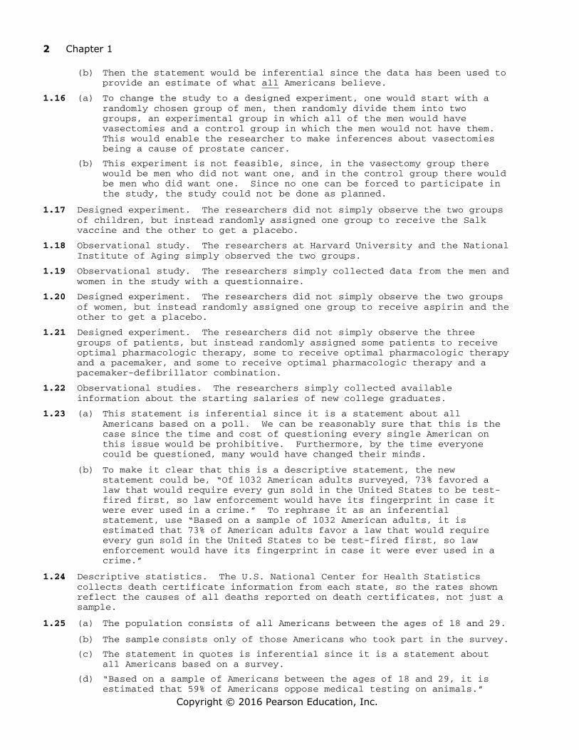
(b) Then the statement would be inferential since the data has been used to provide an estimate of what all Americans believe.
1.16 (a) To change the study to a designed experiment, one would start with a randomly chosen group of men, then randomly divide them into two groups, an experimental group in which all of the men would have vasectomies and a control group in which the men would not have them. This would enable the researcher to make inferences about vasectomies being a cause of prostate cancer.
(b) This experiment is not feasible, since, in the vasectomy group there would be men who did not want one, and in the control group there would be men who did want one. Since no one can be forced to participate in the study, the study could not be done as planned.
1.17 Designed experiment. The researchers did not simply observe the two groups of children, but instead randomly assigned one group to receive the Salk vaccine and the other to get a placebo.
1.18 Observational study. The researchers at Harvard University and the National Institute of Aging simply observed the two groups.
1.19 Observational study. The researchers simply collected data from the men and women in the study with a questionnaire.
1.20 Designed experiment. The researchers did not simply observe the two groups of women, but instead randomly assigned one group to receive aspirin and the other to get a placebo.
1.21 Designed experiment. The researchers did not simply observe the three groups of patients, but instead randomly assigned some patients to receive optimal pharmacologic therapy, some to receive optimal pharmacologic therapy and a pacemaker, and some to receive optimal pharmacologic therapy and a pacemaker-defibrillator combination.
1.22 Observational studies. The researchers simply collected available information about the starting salaries of new college graduates.
1.23 (a) This statement is inferential since it is a statement about all Americans based on a poll. We can be reasonably sure that this is the case since the time and cost of questioning every single American on this issue would be prohibitive. Furthermore, by the time everyone could be questioned, many would have changed their minds.
(b) To make it clear that this is a descriptive statement, the new statement could be, “Of 1032 American adults surveyed, 73% favored a law that would require every gun sold in the United States to be test-fired first, so law enforcement would have its fingerprint in case it were ever used in a crime.” To rephrase it as an inferential statement, use “Based on a sample of 1032 American adults, it is estimated that 73% of American adults favor a law that would require every gun sold in the United States to be test-fired first, so law enforcement would have its fingerprint in case it were ever used in a crime.”
1.24 Descriptive statistics. The U.S. National Center for Health Statistics collects death certificate information from each state, so the rates shown reflect the causes of all deaths reported on death certificates, not just a sample.
1.25 (a) The population consists of all Americans between the ages of 18 and 29.
(b) The sample consists only of those Americans who took part in the survey. (c) The statement in quotes is inferential since it is a statement about
all Americans based on a survey.
(d) “Based on a sample of Americans between the ages of 18 and 29, it is estimated that 59% of Americans oppose medical testing on animals.”
Section 1.2 3
Copyright © 2016 Pearson Education, Inc.
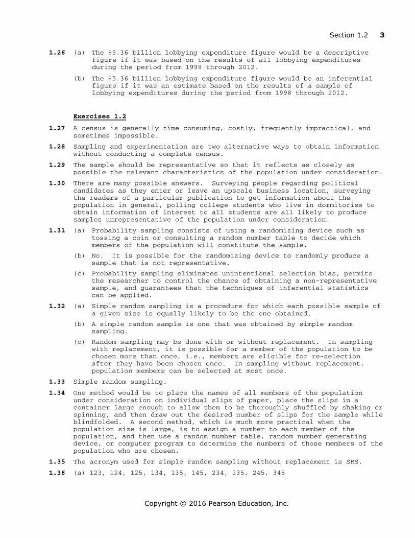
1.26 (a) The $5.36 billion lobbying expenditure figure would be a descriptive figure if it was based on the results of all lobbying expenditures during the period from 1998 through 2012.
(b) The $5.36 billion lobbying expenditure figure would be an inferential figure if it was an estimate based on the results of a sample of lobbying expenditures during the period from 1998 through 2012.
Exercises 1.2
1.27 A census is generally time consuming, costly, frequently impractical, and sometimes impossible.
1.28 Sampling and experimentation are two alternative ways to obtain information without conducting a complete census.
1.29 The sample should be representative so that it reflects as closely as possible the relevant characteristics of the population under consideration.
1.30 There are many possible answers. Surveying people regarding political candidates as they enter or leave an upscale business location, surveying the readers of a particular publication to get information about the population in general, polling college students who live in dormitories to obtain information of interest to all students are all likely to produce samples unrepresentative of the population under consideration.
1.31 (a) Probability sampling consists of using a randomizing device such as tossing a coin or consulting a random number table to decide which members of the population will constitute the sample.
(b) No. It is possible for the randomizing device to randomly produce a sample that is not representative.
(c) Probability sampling eliminates unintentional selection bias, permits the researcher to control the chance of obtaining a non-representative sample, and guarantees that the techniques of inferential statistics can be applied.
1.32 (a) Simple random sampling is a procedure for which each possible sample of a given size is equally likely to be the one obtained.
(b) A simple random sample is one that was obtained by simple random sampling.
(c) Random sampling may be done with or without replacement. In sampling with replacement, it is possible for a member of the population to be chosen more than once, i.e., members are eligible for re-selection after they have been chosen once. In sampling without replacement, population members can be selected at most once.
1.33 Simple random sampling.
1.34 One method would be to place the names of all members of the population under consideration on individual slips of paper, place the slips in a container large enough to allow them to be thoroughly shuffled by shaking or spinning, and then draw out the desired number of slips for the sample while blindfolded. A second method, which is much more practical when the population size is large, is to assign a number to each member of the population, and then use a random number table, random number generating device, or computer program to determine the numbers of those members of the population who are chosen.
1.35 The acronym used for simple random sampling without replacement is SRS.
1.36 (a) 123, 124, 125, 134, 135, 145, 234, 235, 245, 345

4 Chapter 1
Copyright © 2016 Pearson Education, Inc.
(b) There are 10 samples, each of size three. Each sample has a one in 10 chance of being selected. Thus, the probability that a sample of three is 1, 3, and 5 is 1/10.
(c) Starting in Line 05 and column 20, reading single digit numbers down the column and then up the next column, the first digit that is a one through five is a 5. Ignoring duplicates and skipping digits 6 and above and also skipping zero, the second digit found that is a one through five is a 4. Continuing down column 20 and then up column 21, the third digit found that is a one through five is a 1. Thus the SRS of 1,4, and 5 is obtained.
1.37 (a) 12, 13, 14, 23, 24, 34
(b) There are 6 samples, each of size two. Each sample has a one in six chance of being selected. Thus, the probability that a sample of two is 2 and 3 is 1/6.
(c) Starting in Line 17 and column 07 (notice there is a column 00), reading single digit numbers down the column and then up the next column, the first digit that is a one through four is a 1. Continue down column 07 and then up column 08. Ignoring duplicates and skipping digits 5 and above and also skipping zero, the second digit found that is a one through four is a 4. Thus the SRS of 1 and 4 is obtained.
1.38 (a) Starting in Line 15 and reading two digits numbers in columns 25 and 26 going down the table, the first two digit number between 01 and 90 is 06. Continuing down the columns and ignoring duplicates and numbers 91-99, the next two numbers are 33 and 61. Then, continuing up columns 27 and 28, the last two numbers selected are 56 and 20. Therefore the SRS of size five consists of observations 06, 33, 61, 56, and 20.
(b) There are many possible answers.
1.39 (a) Starting in Line 10 and reading two digits numbers in columns 10 and 11 going down the table, the first two digit number between 01 and 50 is 43. Continuing down the columns and ignoring duplicates and numbers 51-99, the next two numbers are 45 and 01. Then, continuing up columns 12 and 13, the last three numbers selected are 42, 37, and 47. Therefore the SRS of size six consists of observations 43, 45, 01, 42, 37, and 47.
(b) There are many possible answers.
1.40 The online poll clearly has a built-in non-response bias. Since it was taken over the Memorial Day weekend, most of those who responded were people who stayed at home and had access to their computers. Most people vacationing outdoors over the weekend would not have carried their computers with them and would not have been able to respond.
1.41 Dentists form a high-income group whose incomes are not representative of the incomes of Seattle residents in general.
1.42 (a) The five possible samples of size one are G, L, S, A, and T.
(b) There is no difference between obtaining a SRS of size 1 and selecting one official at random.
(c) The one possible sample of size five is GLSAT.
(d) There is no difference between obtaining a SRS of size 5 and taking a census of the five officials.
1.43 (a) GLS, GLA, GLT, GSA, GST, GAT, LSA, LST, LAT, SAT.
(b) There are 10 samples, each of size three. Each sample has a one in 10 chance of being selected. Thus, the probability that a sample of three officials is the first sample on the list presented in part (a) is 1/10. The same is true for the second sample and for the tenth sample.

Section 1.2 5
Copyright © 2016 Pearson Education, Inc.
1.44 (a) E,M E,A M,L P,L L,A
E,P E,B M,A P,A L,B
E,L M,P M,B P,B A,B
(b) One procedure for taking a random sample of two representatives from the six is to write the initials of the representatives on six separate pieces of paper, place the six slips of paper into a box, and then, while blindfolded, pick two of the slips of paper. Or, number the representatives 1-6, and use a table of random numbers or a random-number generator to select two different numbers between 1 and 6.
(c) 1/15; 1/15
1.45 (a) E,M,P,L E,M,L,B E,P,A,B M,P,A,B
E,M,P,A E,M,A,B E,L,A,B M,L,A,B
E,M,P,B E,P,L,A M,P,L,A P,L,A,B
E,M,L,A E,P,L,B M,P,L,B
(b) One procedure for taking a random sample of four representatives from the six is to write the initials of the representatives on six separate pieces of paper, place the six slips of paper into a box, and then, while blindfolded, pick four of the slips of paper. Or, number the representatives 1-6, and use a table of random numbers or a random-number generator to select four different numbers between 1 and 6.
(c) 1/15; 1/15
1.46 (a) E,M,P E,P,A M,P,L M,A,B
E,M,L E,P,B M,P,A P,L,A
E,M,A E,L,A M,P,B P,L,B
E,M,B E,L,B M,L,A P,A,B
E,P,L E,A,B M,L,B L,A,B
(b) One procedure for taking a random sample of three representatives from the six is to write the initials of the representatives on six separate pieces of paper, place the six slips of paper into a box, and then, while blindfolded, pick three of the slips of paper. Or, number the representatives 1-6, and use a table of random numbers or a random-number generator to select three different numbers between 1 and 6.
(c) 1/20; 1/20
1.47 (a) F,T F,G F,H F,L F,B F,A
T,G T,H T,L T,B T,A G,H
G,L G,B G,A H,L H,B H,A
L,B L,A B,A
(b) 1/21; 1/21
1.48 (a) I am using Table I to obtain a list of 20 different random numbers between 1 and 80 as follows.
I start at the two digit number in line number 5 and column numbers 31-32, which is the number 86. Since I want numbers between 1 and 80 only, I throw out numbers between 81 and 99, inclusive. I also discard the number 00.
I now go down the table and record the two-digit numbers appearing directly beneath 86.
After skipping 86, I record 39, 03, skip 97, record 28, 58, 59, skip 81, record 09, 36, skip 81, record 52, skip 94, record 24 and 78.

6 Chapter 1
Copyright © 2016 Pearson Education, Inc.
Now that I've reached the bottom of the table, I move directly rightward to the adjacent column of two-digit numbers and go up.
I skip 84, record 57, 40, skip 89, record 69, 25, skip 95, record 51, 20, 42, 77, skip 89, skip 40(duplicate), record 14, and 34.
I've finished recording the 20 random numbers. In summary, these are
39 03 28 58 59
09 36 52 24 78
57 40 69 25 51
20 42 77 14 34
(b) We can use Minitab to generate random numbers. Following the instructions in The Technology Center, our results are 55, 47, 66, 2, 72, 56, 10, 31, 5, 19, 39, 57, 44, 60, 23, 34, 43, 9, 49, and 62. Your result may be different from ours.
1.49 (a) I am using Table I to obtain a list of 10 random numbers between 1 and 500 as follows.
I start at the three digit number in line number 14 and column numbers 10-12, which is the number 452.
I now go down the table and record the three-digit numbers appearing directly beneath 452. Since I want numbers between 1 and 500 only, I throw out numbers between 501 and 999, inclusive. I also discard the number 000.
After 452, I skip 667, 964, 593, 534, and record 016.
Now that I've reached the bottom of the table, I move directly rightward to the adjacent column of three-digit numbers and go up.
I record 343, 242, skip 748, 755, record 428, skip 852, 794, 596, record 378, skip 890, record 163, skip 892, 847, 815, 729, 911, 745, record 182, 293, and 422.
I've finished recording the 10 random numbers. In summary, these are:
452 016 343 242 428
378 163 182 293 422
(b) We can use Minitab to generate random numbers. Following the instructions in The Technology Center, our results are 489, 451, 61, 114, 389, 381, 364, 166, 221, and 437. Your result may be different from ours.
1.50 (a) First assign the digits 0 though 9 to the ten cities as listed in the
exercise. Select a random starting point in Table I of Appendix A and read in a pre-selected direction until you have encountered 5 different digits. For example, if we start at the top of the fifth column of digits and read down, we encounter the digits 4,1,5,2,5,6. We ignore the second ‘5’. Thus our sample of five cities consists of Osaka, Tokyo, Miami, San Francisco, and New York. Your answer may be different from this one.
(b) We can use Minitab to generate random numbers. Following the instructions in The Technology Center, our results are 3, 8, 6, 5, 9. Thus our sample of 5 cities is Los Angeles, Manila, New York, Miami, and London. Your result may be different from ours.
1.51 (a) First re-assign the elements 93 though 118 as elements 01 to 26.
Select a random starting point in Table I of Appendix A and read in a pre-selected direction until you have encountered 8 different elements. For example, if we start at the top of the column 10 and read two digit numbers down and then up in the following columns, we encounter
Section 1.3 7
Copyright © 2016 Pearson Education, Inc.
the elements 04, 01, 03, 08, 11, 18, 22, and 15. This corresponds to a sample of the elements Cm, Np, Am, Fm, Lr, Ds, Fl, and Bh. Your answer may be different from this one.
(b) We can use Minitab to generate random numbers. Following the instructions in The Technology Center, our results are 8, 2, 9, 20, 24, 19, 21, and 13. Thus our sample of 8 elements is Fm, Pu, Md, Cn, Lv, Rg, Uut, and Db. Your result may be different from ours.
1.52 (a) One of the biggest reasons for undercoverage in household surveys is that respondents do not correctly indicate all who are living in a household maybe due to deliberate concealment or irregular household structure or living arrangements. The household residents are only partially listed.
(b) A telephone survey of Americans from a phone book will likely have bias due to undercoverage because many people have unlisted phone numbers and also it is becoming more popular that many people do not even have home phones. This would cause the phone book to be an incomplete list of the population.
1.53 (a) One of the dangers of nonresponse is that the individuals who do not respond may have a different observed value than the individuals that do respond causing a nonresponse bias in the estimate. Nonresponse bias may make the measured value too small or too large.
(b) The lower the response rate, the more likely there is a nonresponse bias in the estimate. Therefore the estimate will either under or over estimate the generalized results to the entire population.
1.54 (a) The respondent may wish to please the questioner by answering what is morally or legally right. The respondent might not be willing to admit to the questioner that they smoke marijuana and the measured value of the percentage of people that smoke marijuana would then be underestimated due to response bias.
(b) Another situation that might be conducive to response bias is perhaps a woman questioning men on their opinion of domestic violence, or an environmentalist questioning people on their recycling habits.
(c) The wording of a question could lead to response bias. Whether the survey is anonymous or not could lead to response bias. The characteristics of the questioner could lead to response bias. It could also happen if the questioner obviously favors and is pushing for one particular answer.
Exercises 1.3
1.55 Systematic random sampling is easier to execute than simple random sampling and usually provides comparable results. The exception is the presence of some kind of cyclical pattern in the listing of the members of the population.
1.56 Ideally, in cluster sampling, each cluster should pattern the entire population.
1.57 Ideally, in stratified sampling, the members of each stratum should be homogeneous relative to the characteristic under consideration.
1.58 Surveys that combine one or more of simple random sampling, systematic random sampling, cluster sampling, and stratified sampling employ what is called multistage sampling.
1.59 (a) Answers will vary, but here is the procedure: (1) Divide the population size, 372, by the sample size, 5, and round down to the nearest whole number if necessary; this gives 74. Use a table of random numbers (or a similar device) to select a number between 1 and 74, call it k. (3) List every 74th number, starting with k, until 5 numbers are obtained;

8 Chapter 1
Copyright © 2016 Pearson Education, Inc.
thus, the first number of the required list of 5 numbers is k, the second is k + 74, the third is k + 148, and so forth.
(b) Following part (a) with k = 10, the first number of the sample is 10, the second is 10 + 74 = 84. The remaining three numbers in the sample would be 158, 232, and 306. Thus, the sample of 5 would be 10, 84, 158, 232, and 306.
1.60 (a) Answers will vary, but here is the procedure: (1) Divide the population size, 500, by the sample size, 9, and round down to the nearest whole number if necessary; this gives 55. Use a table of random numbers (or a similar device) to select a number between 1 and 55, call it k. (3) List every 55th number, starting with k, until 9 numbers are obtained; thus, the first number of the required list of 9 numbers is k, the second is k + 55, the third is k + 110, and so forth.
(b) Following part (a) with k = 48, the first number of the sample is 48, the second is 48 + 55 = 103. The remaining seven numbers in the sample would be 158, 213, 268, 323, 378, 433, and 488. Thus, the sample of 9 would be 48, 103, 158, 213, 268, 323, 378, 433, and 488.
1.61 (a) Answers will vary, but here is the procedure: (1) The population of size 50 is already divided into five clusters of size 10. (2) Since the required sample size is 20, we will need to take a SRS of 2 clusters. Use a table of random numbers (or a similar device) to select two numbers between 1 and 5. These are the two clusters that are selected. (3) Use all the members of each cluster selected in part (2) as the sample.
(b) Following part (a) with clusters #1 and #3 selected, we would select all the members in cluster 1, which are 1 – 10, and all the members in cluster 3, which are 21 – 30.
1.62 (a) Answers will vary, but here is the procedure: (1) The population of size 100 is already divided into ten clusters of size 10. (2) Since the required sample size is 30, we will need to take a SRS of 3 clusters. Use a table of random numbers (or a similar device) to select three numbers between 1 and 10. These are the three clusters that are selected. (3) Use all the members of each cluster selected in part (2) as the sample.
(b) Following part (a) with clusters #2, #6, and #9 selected, we would select all the members in cluster 2 (11-20), all the members in cluster 6 (51-60), and all the members in cluster 9 (81-90). Therefore, our sample would consist of 11-20, 51-60, and 81-90.
1.63 (a) From each strata, we need to obtain a SRS of a size proportional to the size of the stratum. Therefore, since strata #1 is 30% of the population, a SRS equal to 30% of 20, or 6, should be sampled from strata #1. Since strata #2 is 20% of the population, a SRS equal to 20% of 20, or 4, should be sampled from strata #2. Similarly, a SRS of size 8 should be sampled from strata #3 and a SRS of size 2 should be sampled from strata #4. The sample sizes from stratum #1 through #4 are 6, 4, 8, and 2 respectively.
(b) Answers will vary following the procedure in part (a).
1.64 (a) From each strata, we need to obtain a SRS of a size proportional to the size of the stratum. Therefore, since strata #1 is 40% of the population, a SRS equal to 40% of 10, or 4, should be sampled from strata #1. Since strata #2 is 30% of the population, a SRS equal to 30% of 10, or 3, should be sampled from strata #2. Similarly, a SRS of size 3 should be sampled from strata #3. The sample sizes from stratum #1 through #3 are 4, 3, and 3 respectively.
(b) Answers will vary following the procedure in part (a).

Section 1.3 9
Copyright © 2016 Pearson Education, Inc.
1.65 Stratified Sampling. The entire population is naturally divided into subpopulations, one from each lake, and random sampling is done from each lake. The stratified sampling is not with proportional allocation since that would require knowing how many fish were in each lake.
1.66 Stratified Sampling. The entire population is naturally divided into four subpopulations, and random sampling is done from each and then combined into a single sample.
1.67 Systematic Random Sampling. Kennedy selected his sample using the fixed periodic interval of every 50th letter, which is the similar to the method presented in procedure 1.1.
1.68 Cluster Sampling. The clusters of this sampling design are the 1285 journals. A random sample of 26 clusters was selected and then all articles from the selected journals for a particular year were examined.
1.69 Cluster Sampling. The clusters of this sampling design are the 46 schools. A random sample of 10 clusters was selected and then all of the parents of the nonimmunized children at the 10 selected schools were sent a questionnaire.
1.70 Systematic Random Sampling. This sampling design follows procedure 1.1. First, dividing the population size of 8493 by 30, they arrived at k = 283. Then, the randomly selected starting point was m = 10. Then, the sampled stickers were m = 10, m + k = 293, m + 2k = 576, etc.
1.71 (a) Answers will vary, but here is the procedure: (1) Divide the population size, 500, by the sample size, 10, and round down to the nearest whole number if necessary; this gives 50. (2) Use a table of random numbers (or a similar device) to select a number between 1 and 50, call it k. (3) List every 50th, starting with k, until 10 numbers are obtained; thus, the first number on the required list of 10 numbers is k, the second is k+50, the third is k+100, and so forth (e.g., if k=6, then the numbers on the list are 6, 56, 106, ...).
(b) Systematic random sampling is easier.
(c) The answer depends on the purpose of the sampling. If the purpose of sampling is not related to the size of the sales outside the U.S., systematic sampling will work. However, since the listing is a ranking by amount of sales, if k is low (say 2), then the sample will contain firms that, on the average, have higher sales outside the U.S. than the population as a whole. If the k is high, (say 49) then the sample will contain firms that, on the average, have lower sales than the population as a whole. In either of those cases, the sample would not be representative of the population in regard to the amount of sales outside the U.S.
1.72 (a) Answers will vary, but here is the procedure: (1) Divide the population size, 80, by the sample size, 20, and round down to the nearest whole number if necessary; this gives 4. (2) Use a table of random numbers (or a similar device) to select a number between 1 and 4, call it k. (3) List every 4th number, starting with k, until 20 numbers are obtained; thus the first number on the required list of 20 numbers is k, the second is k+4, the third is k+8, and so forth (e.g., if k=3, then the numbers on the list are 3, 7, 11, 15, ...).
(b) Systematic random sampling is easier.
(c) No. In Keno, you want every set of 20 balls to have the same chance of being chosen. Systematic sampling would give each of 4 sets of balls [(1, 5, 9,...,77), (2, 6, 10,...,78), (3, 7, 11,...,79) and (4, 8, 12,...,80)], a 1/4 chance of occurring, while all of the other possible sets of balls would have no chance of occurring.
10 Chapter 1
Copyright © 2016 Pearson Education, Inc.
1.73 (a) Number the suites from 1 to 48, use a table of random numbers to randomly select three of the 48 suites, and take as the sample the 24 dormitory residents living in the three suites obtained.
(b) Probably not, since friends are more likely to have similar opinions than are strangers.
(c) There are 384 students in total. Freshmen make up 1/3 of them. Sophomores make up 7/24 of them, Juniors 1/4, and Seniors 1/8. Multiplying each of these fractions by 24 yields the proportional allocation, which dictates that the number of freshmen, sophomores, juniors, and seniors selected should be, respectively, 8, 7, 6, and 3. Thus a stratified sample of 24 dormitory residents can be obtained as follows: Number the freshmen dormitory residents from 1 to 128 and use a table of random numbers to randomly select 8 of the 128 freshman dormitory residents; number the sophomore dormitory residents from 1 to 112 and use a table of random numbers to randomly select 7 of the 112 sophomore dormitory residents; and so forth.
1.74 (a) Each category of “Percent free lunch” should be represented in the sample in the same proportion that it is present in the population of top 100 ranked high schools. Thus 50/100 of the sample of 25 schools should be from the 0 to under 10% free lunch category, 18/100 from the second category, 11/100 from the third, 8/100 from the fourth, and 13/100 from the last. Multiplying each of these fractions by 25 gives us the sample sizes from each category. These sample sizes will not necessarily be integers, so we will need to make some minor adjustments of the results. The first category should have (50/100)(25) = 12.5. The second should have (18/100)(25) = 4.5. Similarly, the third, fourth, and fifth categories should have 2.75, 2, and 3.25 for their sample sizes. We round the third and fifth sample sizes each to 3. After flipping a coin, we round the first two categories to 12 and 5. Thus the sample sizes for the five Percent free lunch categories should be 12, 5, 3, 2, and 3 respectively. We would now use a random number generator to select 12 out of the 50 in the first category, 5 out of the 18 in the second, 3 out of the 11 in the third, 2 of the 8 in the fourth, and 3 of the 13 in the last category.
(b) From part (a), two schools would be selected from the strata with a percent free lunch value of 30-under 40.
1.75 (a) Answers will vary, but here is the procedure: (1) Divide the population size, 435, by the sample size, 15, and round down to the nearest whole number if necessary; this gives 29. Use a table of random numbers (or a similar device) to select a number between 1 and 29, call it k. (3) List every 29th number, starting with k, until 15 numbers are obtained; thus, the first number of the required list of 15 numbers is k, the second is k + 29, the third is k + 58, and so forth.
(b) Following part (a) with k = 12, the first number of the sample is 12, the second is 12 + 29 = 41. The third number selected is 12 + 58 = 70. The remaining twelve numbers are similarly selected. Thus, the sample of 15 would be 12, 41, 70, 99, 128, 157, 186, 215, 244, 273, 302, 331, 360, 389, and 418.
1.76 (a) Each category of “Region” should be represented in the sample in the same proportion that it is present in the population. Thus 43% of the sample of 50 should be volunteers serving in Africa, 21% from Latin America, 15% from Eastern Europe/Central Asia, 10% from Asia, 4% from the Caribbean, 4% from North Africa/Middle East, and 3% from the Pacific Island. Finding each of these proportions of 50 gives us the sample sizes from each category. These sample sizes will not necessarily be integers, so we will need to make some minor adjustments of the results. Volunteers from Africa should have (0.43)(50) = 21.5. Volunteers from Latin America should have (0.21)(50) = 10.5.

Section 1.3 11
Copyright © 2016 Pearson Education, Inc.
Similarly, the remaining categories should have 7.5, 5, 2, 2, and 1.5 for their sample sizes. After flipping a coin, we round the first two categories either up or down. Thus the sample sizes for the categories should be 21, 11, 7, 5, 2, 2, and 2 respectively. We would now use a random number generator to select the volunteers from each category.
(b) From part (a), two volunteers would be selected from the strata with volunteers serving in the Caribbean.
1.77 (a) This is a poll taken by calling randomly selected U.S. adults. Thus, the sampling design appears to be simple random sampling, although it is possible that a more complex design was used to ensure that various political, religious, educational, or other types of groups were proportionately represented in the sample.
(b) The sample size for the second question was 78% of 1010 or 788.
(c) The sample size for the third question was 28% of 788 or 221.
1.78 No. In your text, Example 1.10, only 48 different samples are possible. A sample containing students 5,6, and 7 is not possible at all. While the 48 possible samples are equally likely, there are other samples that could be obtained through simple random sampling that are not possible at all in systematic sampling. Thus not all possible samples are equally likely. Nevertheless, if there is no pattern or cycle to the data, this method will tend to give about the same results as simple random sampling.
1.79 (a) It is also true for systematic random sampling if the population size divided by the sample size results in an integer for m. The chance for each member to be selected is then still equal to the sample size divided by the population size. For example, suppose the population size is N=10 and the sample size is n=2. The chance that each member in simple random sampling to be selected is 2/10 = 1/5. In systematic random sampling for the same example, m=5. The possible samples of size two are 1 and 6, 2 and 7, 3 and 8, 4 and 9, and 5 and 10. Therefore, the chance that a member is selected is equal to the chance of one of those five samples being selected, which is the same as simple random sampling of 1/5.
(b) It is not true for systematic random sampling if the population size divided by the sample size does not result in an integer for m. For example, suppose the population size is N=15 and the sample size is n=2. After dividing the population size by the sample size and rounding down to the nearest whole number, we get m=7. You would select every 7th member after a random starting place k, between 1 and 7, is determined. If k=1, you would select the first and eighth member. If k=7, you would select the seventh and fourteenth member. In this situation, the last member (fifteenth) can never be selected. Therefore, the last member of the sample does not have the same chance of being selected as any other member in the population.
1.80 Refer to example 1.14. If we approached this problem as a simple random sample each member would have a chance of being selected equal to the sample size divided by the population size: 20/250, or 2/25.
If we approached this same example as a stratified sample with proportional allocation, we would select 2 out of 25 households in the upper income group, 14 out of the 175 households in the middle income group, and 4 out of 50 households in the lower income group. Thus the chance that an upper income household is selected is 2/25. The chance that a middle income household is selected is 14/175 = 2/25. Finally, the chance that a lower income household is selected is 4/50 = 2/25. Thus, the chance that each member is selected is the same as a simple random sample.

12 Chapter 1
Copyright © 2016 Pearson Education, Inc.
Exercises 1.4
1.81 (a) Experimental units are the individuals or items on which the experiment is performed.
(b) When the experimental units are humans, we call them subjects.
1.82 The three basic principles of experimental design are control, randomization, and replication.
Control: Two or more treatments should be compared.
Randomization: The experimental units should be randomly divided into groups to avoid unintentional selection bias in constituting the groups.
Replication: A sufficient number of experimental units should be used to ensure that randomization creates groups that resemble each other closely and to increase the chances of detecting differences among the treatments.
1.83 (a) The response variable is the characteristic of the experimental outcome that is to be measured or observed.
(b) A factor is a variable whose effect on the response variable is of interest in the experiment.
(c) The levels are the possible values of the factor.
(d) For a one-factor experiment, the treatments are the levels of the factor. For multifactor experiments, the treatments are the combinations of levels of the factors.
1.84 One type of statistical design is a completely randomized design. In a completely randomized design, all the experimental units are assigned randomly among all the treatments. The second type of statistical design is a randomized block design. In a randomized block design, the experimental units are assigned randomly among all the treatments separately within each block.
1.85 In a one-factor experiment, the number of treatments is equal to the number of levels of the factor. Therefore, there are four treatments.
1.86 In a one-factor experiment, the number of treatments is equal to the number of levels of the factor. Therefore, there are five treatments.
1.87 (a)
B b1 b2 b3 b4
A
a1 a1b1 a1b2 a1b3 a1b4
a2 a2b1 a2b2 a2b3 a2b4
a3 a3b1 a3b2 a3b3 a3b4
(b) There are twelve combinations of the levels of the factors. Therefore, there are twelve treatments.
(c) Yes, you could have multiplied the number of levels in each factor. There are three levels of factor A and four levels of factor B. Therefore, there are (3)(4) = 12 treatments.

Section 1.4 13
Copyright © 2016 Pearson Education, Inc.
1.88 (a)
B b1 b2
A
a1 a1b1 a1b2
a2 a2b1 a2b2
a3 a3b1 a3b2
a4 a4b1 a4b2
(b) There are eight combinations of the levels of the factors. Therefore, there are eight treatments.
(c) Yes, you could have multiplied the number of levels in each factor. There are four levels of factor A and two levels of factor B. Therefore, there are (4)(2) = 8 treatments.
1.89 You can multiply the number of levels in each factor. There are m levels in the first factor and n levels in the second factor. Therefore, there are (m)(n) = m n× treatments.
1.90 (a) The treatment group consisted of the 2444 patients who took Prozac.
(b) The control group consisted of the 1331 patients who received a placebo.
(c) The treatments were administering Prozac and administering the placebo.
1.91 (a) There were three treatments.
(b) The first group, the one receiving only the pharmacologic therapy, would be considered the control group.
(c) There were three treatment groups. The first received only pharmacologic therapy, the second received pharmacologic therapy plus a pacemaker, and the third received pharmacologic therapy plus a pacemaker-defibrillator combination.
(d) The first group (control) contained 1/5 of the 1520 patients or 304. The other two groups each contained 2/5 of the 1520 patients or 608.
(e) Each patient could be randomly assigned a number from 1 to 1520. Any patient assigned a number between 1 and 304 would be assigned to the control group; any patient assigned to the next 608 numbers (305 to 912) would be assigned to receive the pharmacologic therapy plus a pacemaker; and any patient assigned a number between 913 and 1520 would receive pharmacologic therapy plus a pacemaker-defibrillator combination. Each random number would be used only once to ensure that the resulting treatment groups were of the intended sizes.
1.92 (a) Experimental units: batches of the product being sold
(b) Response variable: the number of units of the product sold
(c) Factors: two factors - display type and pricing scheme
(d) Levels of each factor: three types of display of the product and three pricing schemes
(e) Treatments: the nine different combinations of display type and price resulting from testing each of the three pricing schemes with each of the three display types
1.93 (a) Experimental units: the drivers
(b) Response variable: the detection distance, in feet
(c) Factors: two factors – sign size and sign material

14 Chapter 1
Copyright © 2016 Pearson Education, Inc.
(d) Levels of each factor: three levels of sign size (small, medium, and large) and three levels of sign material (1, 2, and 3)
(e) Treatments: the nine different combinations of sign size and sign material resulting from testing each of the three sign sizes with each of the three sign materials
1.94 (a) Experimental units: fields of oats
(b) Response variable: crop yield of the oats per acre
(c) Factors: variety of oats and concentration of manure on the fields
(d) Levels of each factor: three varieties of oats and four concentrations of manure
(e) Treatments: the twelve combinations of oat variety and manure concentration resulting from testing each of the three oat varieties with each of the four concentration levels of the manure
1.95 (a) Experimental units: female lions
(b) Response variable: whether or not the female lion approached the male lion dummy
(c) Factors: length and color of the mane on the male lion dummy
(d) Levels of each factor: two different mane lengths and two different mane colors
(e) Treatments: the four combinations of mane length and color
1.96 (a) Experimental units: the women in the study
(b) Response variable: the color of the shirt chosen
(c) Factors: gender and attractiveness of the new acquaintance
(d) Levels of each factor: two different genders (male, female) and two different levels of attractiveness (attractive, unattractive)
(e) Treatments: the four combinations of gender and attractiveness
1.97 (a) Experimental units: the children
(b) Response variable: IQ score
(c) Factor: Whether they were given dexamethasone (control or dexamethasone group)
(d) Levels of each factor: two levels of the single factor (control or dexamethasone group)
(e) Treatments: the two levels of the single factor
1.98 (a) This is a completely randomized design since the flashlights were randomly assigned to the different battery brands.
(b) This is a randomized block design since the four different battery brands would be randomly assigned within each set of four flashlights from each of the five flashlight brands.
1.99 (a) This is a randomized block design. The experiment first blocked by gender. All the experimental units are not randomly assigned among all the treatments.
(b) The blocks are the two genders (male and female).
1.100 Double-blinding guards against bias, both in the evaluations and in the responses. In the Salk vaccine experiment, double-blinding prevented a doctor's evaluation from being influenced by knowing which treatment (vaccine or placebo) a patient received; it also prevented a patient's response to the treatment from being influenced by knowing which treatment he or she received.

Review Problems 15
Copyright © 2016 Pearson Education, Inc.
1.101 (a) Simple random sampling corresponds to completely randomized designs since selection is randomly made from the entire population.
(b) Stratified sampling corresponds to randomized block designs since selection is randomly made from within each strata.
Review Problems for Chapter 1
1. Student exercise.
2. Descriptive statistics are used to display and summarize the data to be used in an inferential study. Preliminary descriptive analysis of a sample often reveals features of the data that lead to the choice or reconsideration of the choice of the appropriate inferential analysis procedure.
3. (a) An observational study is a study in which researchers simply observe characteristics and take measurements.
(b) A designed experiment is a study in which researchers impose treatments and controls and then observe characteristics and take measurements.
4. A literature search should be made before planning and conducting a study.
5. (a) A representative sample is one that reflects as closely as possible the relevant characteristics of the population under consideration.
(b) Probability sampling involves the use of a randomizing device such as tossing a coin or die, using a random number table, or using computer software that generates random numbers to determine which members of the population will make up the sample.
(c) A sample is a simple random sample if all possible samples of a given size are equally likely to be the actual sample selected.
6. (a) This method does not involve probability sampling. No randomizing device is being used and people who do not visit the campus cafeteria have no chance of being included in the sample.
(b) The dart throwing is a randomizing device that makes all samples of size 20 equally likely. This is probability sampling.
7. (a) Systematic random sampling is done by first dividing the population size by the sample size and rounding the result down to the next integer, say m. Then we select one random number, say k, between 1 and m inclusive. That number will be the first member of the sample. The remaining members of sample will be those numbered k+m, k+2m, k+3m, ... until a sample of size n has been chosen. Systematic sampling will yield results similar to simple random sampling as long as there is nothing systematic about the way the members of the population were assigned their numbers.
(b) In cluster sampling, clusters of the population (such as blocks, precincts, wards, etc.) are chosen at random from all such possible clusters. Then every member of the population lying within the chosen clusters is sampled. This method of sampling is particularly convenient when members of the population are widely scattered and is most appropriate when the members of each cluster are representative of the entire population. Cluster sampling can save both time and expense in doing the survey, but can yield misleading results if individual clusters are made up of subjects with very similar views on the topic being surveyed.
(c) In stratified random sampling with proportional allocation, the population is first divided into subpopulations, called strata, and simple random sampling is done within each stratum. Proportional allocation means that the size of the sample from each stratum is proportional to the size of the population in that stratum. This type

16 Chapter 1
Copyright © 2016 Pearson Education, Inc.
of sampling may improve the accuracy of the survey by ensuring that those in each stratum are more proportionately represented than would be the case with cluster sampling or even simple random sampling. Ideally, the members of each stratum should be homogeneous relative to the characteristic under consideration. If they are not homogeneous within each stratum, simple random sampling would work just as well.
8. The three basic principles of experimental design are control, randomization, and replication. Control refers to methods for controlling factors other than those of primary interest. Randomization means randomly dividing the subjects into groups in order to avoid unintentional selection bias in constituting the groups. Replication means using enough experimental units or subjects so that groups resemble each other closely and so that there is a good chance of detecting differences among the treatments when such differences actually exist.
9. Descriptive study. It is a summary of the scores of major league baseball games on August 14, 2013.
10. (a) Descriptive study. It is a summary of the responses from those that participated in the poll.
(b) Inferential statement. It is an implied estimate of the responses of all adults in the U.S.
11. Inferential study. The results of a sample are used to make inferences about the age distribution of all British backpackers in South Africa.
12. (a) Descriptive study. It is a summary of the percentages of Jewish children sampled in Israel and Britain that have peanut allergies.
(b) Observational study. The researchers simply observed the two groups.
13. This is an observational study. To be a designed experiment, the researchers would have to have the ability to assign some children at random to live in persistent poverty during the first 5 years of life or to not suffer any poverty during that period. Clearly that is not possible.
14. This is a designed experiment since the researcher is imposing a treatment and then observing the results.
15. Because Yale is a very expensive school, incomes of parents of Yale students will not be representative of the incomes of all college students’ parents.
16. (a) H,Z,C H,Z,A H,Z,J H,C,A H,C,J
H,A,J Z,C,A Z,C,J Z,A,J C,A,J
(b) Since each of the 10 samples of size three is equally likely, there is a 1/10 chance that the sample chosen is the first sample in the list, 1/10 chance that it is the second sample in the list, and 1/10 chance that it is the tenth sample in the list.
(c) (i) Make five slips of paper with each airline on one slip. Draw three slips at random. (ii) Make 10 slips of paper, each having one of the combinations in part (a). Draw one slip at random. (iii) Number the five airlines from 1 to 5. Use a random number table or random number generator to obtain three distinct random numbers between 1 and 5, inclusive.
(d) Your method and result may differ from ours. We rolled a die (ignoring 6’s and duplicates) and got 2, 5, 2, 6, 4. Ignoring duplicates and numbers greater than five, our sample consists of Horizon, Jazz, and Alaska Airlines.
17. (a) Table I can be employed to obtain a sample of 15 random numbers between 1 and 100 as follows. First, I pick a random starting point by closing my eyes and putting my finger down on the table.

Review Problems 17
Copyright © 2016 Pearson Education, Inc.
My finger falls on three digits located at the intersection of a line with three columns. (Notice that the first column of digits is labeled "00" rather than "01".) This is my starting point.
I now go down the table and record all three-digit numbers appearing directly beneath the first three-digit number that are between 001 and 100 inclusive. I throw out numbers between 101 and 999, inclusive. I also discard the number 0000. When the bottom of the column is reached, I move over to the next sequence of three digits and work my way back up the table. Continue in this manner. When 10 distinct three-digit numbers have been recorded, the sample is complete.
(b) Starting in row 10, columns 7-9, we skip 484, 797, record 082, skip 586, 653, 452, 552, 155, record 008, skip 765, move to the right and record 016, skip 534, 593, 964, 667, 452, 432, 594, 950, 670, record 001, skip 581, 577, 408, 948, 807, 862, 407, record 047, skip 977, move to the right, skip 422 and all of the rest of the numbers in that column, move to the right, skip 732, 192, record 094, skip 615 and all of the rest of the numbers in that column, move to the right, record 097, skip 673, record 074, skip 469, 822, record 052, skip 397, 468, 741, 566, 470, record 076, 098, skip 883, 378, 154, 102, record 003, skip 802, 841, move to the right, skip 243, 198, 411, record 089, skip 701, 305, 638, 654, record 041, skip 753, 790, record 063.
The final list of numbers is 82, 8, 16, 1, 47, 94, 97, 74, 52, 76, 98, 3, 89, 41, 63.
(c) Using Minitab, our results were the numbers 46, 99, 90, 31, 75, 98, 79, 14, 44, 13, 66, 49, 37, 87, 73, 26, 61, 71, 72, 2. Thus our sample consists of the first 15 numbers 46, 99, 90, 31, 75, 98, 79, 14, 44, 13, 66, 49, 37, 87, 73. Your sample may be different.
18. The statement under the vote is a disclaimer as to the validity of the survey. Since the vote reflects only the responses of volunteers who chose to vote, it cannot be regarded as representative of the public in general, some of which do not use the Internet, nor as representative of Internet users since the sample was not chosen at random from either group.
19. The data in this study were clearly not collected via a controlled experiment in which some participants were forced to do crossword puzzles, practice musical instruments, play board games, or read while others were not allowed to do any of those activities. Therefore, any data relative to these activities and dementia arose as a result of observing whether or not the subjects in the study carried out any of those activities and whether or no they had some form of dementia. Since this would be an observational study, no statement of cause and effect can rightfully be made.
20. The researchers did not impose or manipulate any of the conditions of this study. They didn’t decide who had cancer, who didn’t have cancer, who had hepatitis B, or who had hepatitis C. This study was an observational study and not a controlled experiment. Observational studies can only reveal an association, not causation. Therefore, the statement in quotes is valid. If the researchers wanted to establish causation, they would need a designed experiment.
21. (a) Answers will vary, but here is the procedure: (1) Divide the population size, 100, by the sample size 15, and round down to the nearest whole number; this gives 6. (2) Use a table of random numbers (or a similar device) to select a number between 1 and 6, call it k. (3) List every 6th number, starting with k, until 15 numbers are obtained; thus the first number on the required list of 15 numbers is k, the second is k+6, the third is k+12, and so forth (e.g., if k=4, then the numbers on the list are 4, 10, 16, ...).
(b) Yes, unless for some reason there is some kind of trend or a cyclical pattern in the listing of the athletes.

18 Chapter 1
Copyright © 2016 Pearson Education, Inc.
22. (a) Each category of “Distance from Plant” should be represented in the sample in the same proportion that it is present in the population of City of Durham’s water distribution system. 1310/11707 = 0.112. Thus, 11.2% of the sample of 80 water samples should be from “Less than 1.5 miles”, 27.0% from “1.5 – less than 3.0 miles”, 24.1% from “3.0 – less than 4.5 miles”, 13.6% from “4.5 – less than 6.0 miles”, 11.5% from “6.0 – less than 7.5 miles”, and 12.5% from “7.5 miles or greater”. Multiplying each of these fractions by 80 gives us the sample sizes from each category. These sample sizes will not necessarily be integers, so we will need to make some minor adjustments of the results. The first category should have (11.2/100)(80) = 8.96. The second should have (27/100)(80) = 21.6. Similarly, the third, fourth, fifth, and sixth categories should have 19.28, 10.88, 9.2, and 10 for their sample sizes. We round the six sample sizes from the categories to 9, 22, 19, 11, 9, and 10 respectively. We would now randomly select water samples from each region.
23. (a) This is a designed experiment.
(b) The treatment group consists of the 158 patients who took AVONEX. The control group consists of the 143 patients who were given a placebo. The treatments were the AVONEX and the placebo.
24. (a) Experimental units: tomato plants
(b) Response variable: yield of tomatoes
(c) Factor(s): tomato variety and density of plants
(d) Levels of each factor: The four tomato varieties (Harvester, Pusa Early Dwarf, Ife No. 1, and Ibadan Local) would be the levels of variety. The four densities (10,000, 20,000, 30,000, and 40,000 plants/ha) would be the levels of the density.
(e) Treatments: Each treatment would be one of the combinations of a variety planted at a given plant density.
25. (a) Experimental Units: The children
(b) Response variable: Whether or not the child was able to open the bottle
(c) Factors: The container designs
(d) Levels of each factor: Three (types of containers)
(e) Treatments: The container designs
26. This is a completely randomized design. All of the experimental units (batches of doughnuts) were assigned at random to the four treatments (four different fats).
27. (a) This is a completely randomized design since the 24 cars were randomly assigned to the 4 brands of gasoline.
(b) This is a randomized block design. The four different gasoline brands are randomly assigned to the four cars in each of the six car model groups. The blocks are the six groups of four identical cars each.
(c) If the purpose is to learn about the mileage rating of one particular car model with each of the four gasoline brands, then the completely randomized design is appropriate. But if the purpose is to learn about the performance of the gasoline across a variety of cars (and this seems more reasonable), then the randomized block design is more appropriate and will allow the researcher to determine the effect of car model as well as of gasoline type on the mileage obtained.
Case Study 19
Copyright © 2016 Pearson Education, Inc.
Case Study: Top Films of All Time
(a) The population of interest in the AFI survey is the population of film artists, critics, and historians.
(b) The sample is the 1500 film artists, critics, and historians polled.
(c) No. The population of all American moviegoers includes many people who are not film artists, critics, nor historians. Furthermore, these members of the film community have very specialized interests and possibly different viewpoints as to what constitutes a great actor or actress than many others in the American movie-going population.
(d) Descriptive. It merely describes the opinion of those in the sample without trying to draw an inference about the opinions of all moviegoers.
(e) Inferential. This statement would be an attempt to draw an inference about the opinion of all artists, historians, and critics based on the opinions of those 1500 people who were interviewed.

21
Copyright © 2016 Pearson Education, Inc.
CHAPTER 2 SOLUTIONS
Exercises 2.1
2.1 (a) Hair color, model of car, and brand of popcorn are qualitative variables.
(b) Number of eggs in a nest, number of cases of flu, and number of employees are discrete, quantitative variables.
(c) Temperature, weight, and time are quantitative continuous variables.
2.2 (a) A qualitative variable is a nonnumerically valued variable. Its possible “values” are descriptive (e.g., color, name, gender).
(b) A discrete, quantitative variable is one whose possible values can be listed. It is usually obtained by counting rather than by measuring.
(c) A continuous, quantitative variable is one whose possible values form some interval of numbers. It usually results from measuring.
2.3 (a) Qualitative data result from observing and recording values of a qualitative variable, such as, color or shape.
(b) Discrete, quantitative data are values of a discrete quantitative variable. Values usually result from counting something.
(c) Continuous, quantitative data are values of a continuous variable. Values are usually the result of measuring something such as temperature that can take on any value in a given interval.
2.4 The classification of data is important because it will help you choose the correct statistical method for analyzing the data.
2.5 Of qualitative and quantitative (discrete and continuous) types of data, only qualitative yields nonnumerical data.
2.6 (a) The first column consists of quantitative, discrete data. This column provides ranks of the highest recorded temperature for each continent.
(b) The second column consists of qualitative data since continent names are nonnumerical.
(c) The fourth column consists of quantitative, continuous data. This column provides the highest recorded temperatures for the continents in degrees Farenheit.
(d) The information that Death Valley is in the United States is qualitative data since country in which a place is located is nonnumerical.
2.7 (a) The first column consists of quantitative, continuous data. This column provides the time that the earthquake occurred.
(b) The second column consists of quantitative, continuous data. This column provides the magnitude of each earthquake.
(c) The third column consists of quantitative, continuous data. This column provides the depth of each earthquake in kilometers.
(d) The fourth column consists of quantitative, discrete data. This column provides the number of stations that reported activity on the earthquake.
(e) The fifth column consists of qualitative data since the region of the location of each earthquake is nonnumerical.
2.8 (a) The first column consists of quantitative, discrete data. This column provides ranks of the top ten IPOs in the United States.
22 Chapter 2
Copyright © 2016 Pearson Education, Inc.
(b) The second column consists of qualitative data since company names are nonnumerical.
(c) The third column consists of quantitative, discrete data. Since money involves discrete units, such as dollars and cents, the data is discrete, although, for all practical purposes, this data might be considered quantitative continuous data.
(d) The information that Facebook is a social networking business is qualitative data since type of business is nonnumerical.
2.9 (a) The first column consists of quantitative, discrete data. This column provides the ranks of the deceased celebrities with the top 10 earnings.
(b) The second column consists of qualitative data since names are nonnumerical.
(c) The third column consists of quantitative, discrete data, the earnings of the celebrities. Since money involves discrete units, such as dollars and cents, the data is discrete, although, for all practical purposes, this data might be considered quantitative continuous data
2.10 (a) The first column consists of quantitative, discrete data. This column provides the ranks of the top 10 universities for 2012-2013.
(b) The second column consists of qualitative data since names of the institutions are nonnumerical.
(c) The third column consists of quantitative, continuous data. This column provides the overall score of the top 10 universities for 2012-2013.
2.11 (a) The first column contains types of products. They are qualitative data since they are nonnumerical.
(b) The second column contains number of units shipped in the millions. These are whole numbers and are quantitative, discrete.
(c) The third column contains money values. Technically, these are quantitative, discrete data since there are gaps between possible values at the cent level. For all practical purposes, however, these are quantitative, continuous data.
2.12 Player name, team, and position are nonnumerical and are therefore qualitative data. The number of runs batted in, or RBI, are whole numbers and are therefore quantitative, discrete. Weight is quantitative, continuous.
2.13 The first column contains quantitative, discrete data in the form of ranks. These are whole numbers. The second and third columns contain qualitative data in the form of names. The last column contains the rating of the program which is quantitative, continuous.
2.14 The first column is qualitative since it is nonnumerical. The second and third columns are quantitative, discrete since they report the number of grants and applications received. The last column is quantitative, continuous since it reports the success rate of the grants.
2.15 The first column is quantitative, discrete since it is reporting a rank. The second and third columns are qualitative since make/model and type are nonnumerical. The last column is quantitative, continuous since it is reporting mileage.
2.16 Of the eight items presented, only high school class rank involves ordinal data. The rank is ordinal data.

Section 2.2 23
Copyright © 2016 Pearson Education, Inc.
Exercises 2.2
2.17 A frequency distribution of qualitative data is a table that lists the distinct values of data and their frequencies. It is useful to organize the data and make it easier to understand.
2.18 (a) The frequency of a class is the number of observations in the class, whereas, the relative frequency of a class is the ratio of the class frequency to the total number of observations.
(b) The percentage of a class is 100 times the relative frequency of the class. Equivalently, the relative frequency of a class is the percentage of the class expressed as a decimal.
2.19 (a) True. Having identical frequency distributions implies that the total number of observations and the numbers of observations in each class are identical. Thus, the relative frequencies will also be identical.
(b) False. Having identical relative frequency distributions means that the ratio of the count in each class to the total is the same for both frequency distributions. However, one distribution may have twice (or some other multiple) the total number of observations as the other. For example, two distributions with counts of 5, 4, 1 and 10, 8, 2 would be different, but would have the same relative frequency distribution.
(c) If the two data sets have the same number of observations, either a frequency distribution or a relative-frequency distribution is suitable. If, however, the two data sets have different numbers of observations, using relative-frequency distributions is more appropriate because the total of each set of relative frequencies is 1, putting both distributions on the same basis for comparison.
2.20 (a)-(b)
The classes are presented in column 1. The frequency distribution of the classes is presented in column 2. Dividing each frequency by the total number of observations, which is 5, results in each class's relative frequency. The relative frequency distribution is presented in column 3.
Class Frequency Relative Frequency A 2 0.40
B 2 0.40
C 1 0.20
5 1.00
(c) We multiply each of the relative frequencies by 360 degrees to obtain the portion of the pie represented by each class. The result using Minitab is

24 Chapter 2
Copyright © 2016 Pearson Education, Inc.
ABC
Category
C20.0%
B40.0%
A40.0%
Pie Chart
(d) We use the bar chart to show the relative frequency with which each
class occurs. The result is
CBA
40
30
20
1 0
0
Class
Perc
ent
Percent within all data.
Bar Graph
2.21 (a)-(b)
The classes are presented in column 1. The frequency distribution of the classes is presented in column 2. Dividing each frequency by the total number of observations, which is 5, results in each class's relative frequency. The relative frequency distribution is presented in column 3.
Class Frequency Relative Frequency
A 3 0.60
B 1 0.20
C 1 0.20
5 1.00
(c) We multiply each of the relative frequencies by 360 degrees to obtain the portion of the pie represented by each class. The result using Minitab is

Section 2.2 25
Copyright © 2016 Pearson Education, Inc.
ABC
Category
C20.0%
B20.0%
A60.0%
Pie Chart
(d) We use the bar chart to show the relative frequency with which each
class occurs. The result is
CBA
60
50
40
30
20
1 0
0
Class
Perc
ent
Percent within all data.
Bar Graph
2.22 (a)-(b)
The classes are presented in column 1. The frequency distribution of the classes is presented in column 2. Dividing each frequency by the total number of observations, which is 10, results in each class's relative frequency. The relative frequency distribution is presented in column 3.
Class Frequency Relative Frequency A 4 0.40
B 1 0.10
C 1 0.10
D 4 0.40
10 1.00
(c) We multiply each of the relative frequencies by 360 degrees to obtain the portion of the pie represented by each class. The result using Minitab is
26 Chapter 2
Copyright © 2016 Pearson Education, Inc.
ABCD
Category
D40.0%
C10.0%
B10.0%
A40.0%
Pie Chart
(d) We use the bar chart to show the relative frequency with which each
class occurs. The result is
DCBA
40
30
20
1 0
0
Class
Perc
ent
Percent within all data.
Bar Chart
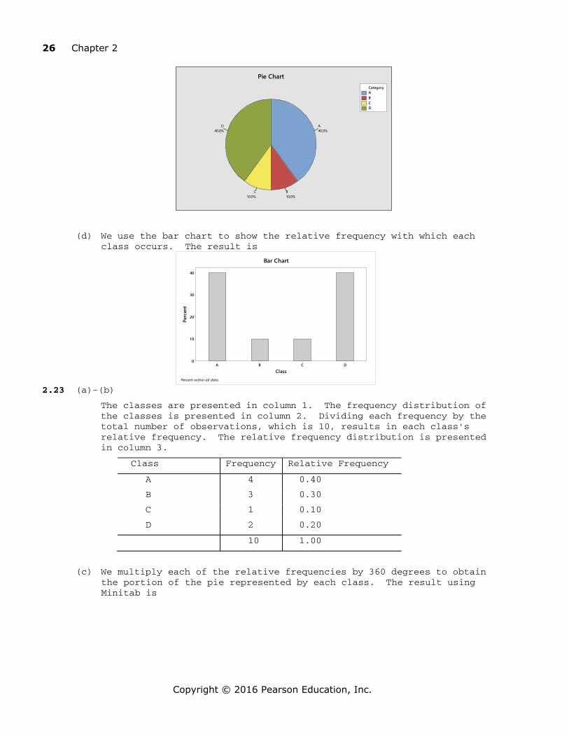
2.23 (a)-(b)
The classes are presented in column 1. The frequency distribution of the classes is presented in column 2. Dividing each frequency by the total number of observations, which is 10, results in each class's relative frequency. The relative frequency distribution is presented in column 3.
Class Frequency Relative Frequency
A 4 0.40
B 3 0.30
C 1 0.10
D 2 0.20
10 1.00
(c) We multiply each of the relative frequencies by 360 degrees to obtain the portion of the pie represented by each class. The result using Minitab is
Section 2.2 27
Copyright © 2016 Pearson Education, Inc.
ABCD
Category
D20.0%
C10.0%
B30.0%
A40.0%
Pie Chart
(d) We use the bar chart to show the relative frequency with which each
class occurs. The result is
DCBA
40
30
20
1 0
0
Class
Perc
ent
Percent within all data.
Bar Chart
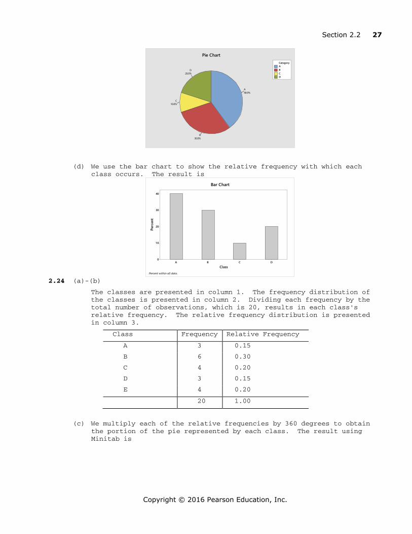
2.24 (a)-(b)
The classes are presented in column 1. The frequency distribution of the classes is presented in column 2. Dividing each frequency by the total number of observations, which is 20, results in each class's relative frequency. The relative frequency distribution is presented in column 3.
Class Frequency Relative Frequency A 3 0.15
B 6 0.30
C 4 0.20
D 3 0.15
E 4 0.20
20 1.00
(c) We multiply each of the relative frequencies by 360 degrees to obtain the portion of the pie represented by each class. The result using Minitab is
28 Chapter 2
Copyright © 2016 Pearson Education, Inc.
ABCDE
Category
E20.0%
D15.0%
C20.0%
B30.0%
A15.0%
Pie Chart
(d) We use the bar chart to show the relative frequency with which each
class occurs. The result is
EDCBA
30
25
20
1 5
1 0
5
0
Class
Perc
ent
Percent within all data.
Bar Chart
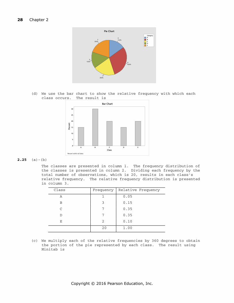
2.25 (a)-(b)
The classes are presented in column 1. The frequency distribution of the classes is presented in column 2. Dividing each frequency by the total number of observations, which is 20, results in each class's relative frequency. The relative frequency distribution is presented in column 3.
Class Frequency Relative Frequency
A 1 0.05
B 3 0.15
C 7 0.35
D 7 0.35
E 2 0.10
20 1.00
(c) We multiply each of the relative frequencies by 360 degrees to obtain the portion of the pie represented by each class. The result using Minitab is
Section 2.2 29
Copyright © 2016 Pearson Education, Inc.
ABCDE
CategoryE
10.0%
D35.0%
C35.0%
B15.0%
A5.0%
Pie Chart
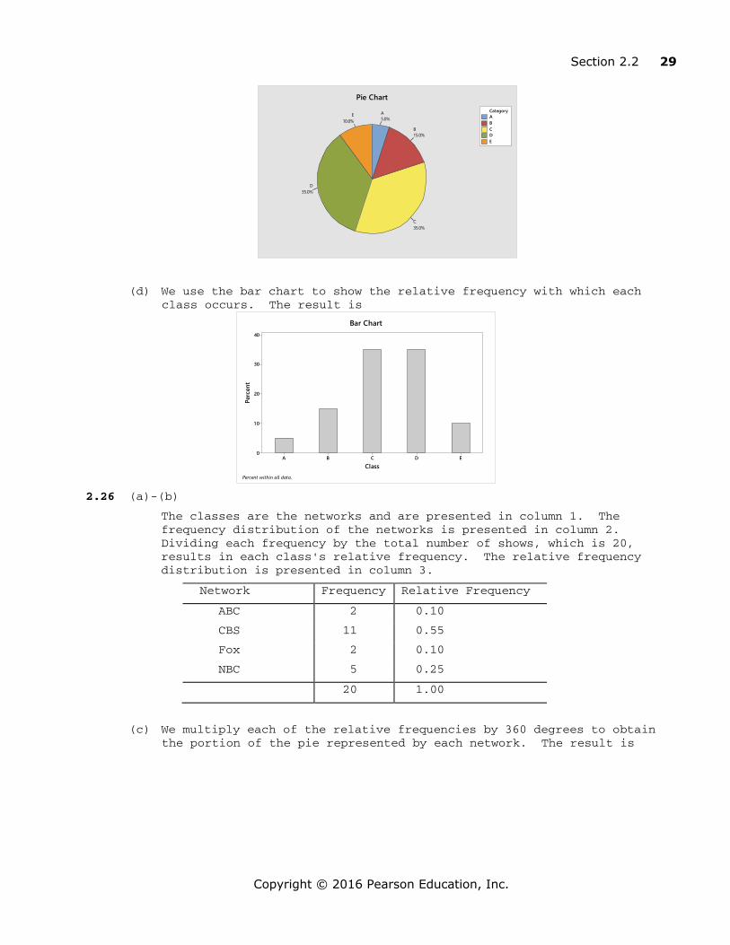
(d) We use the bar chart to show the relative frequency with which each
class occurs. The result is
EDCBA
40
30
20
10
0
Class
Perc
ent
Percent within all data.
Bar Chart
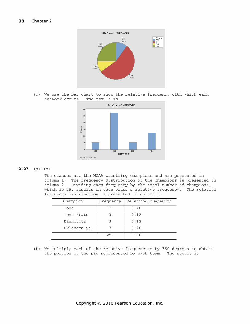
2.26 (a)-(b)
The classes are the networks and are presented in column 1. The frequency distribution of the networks is presented in column 2. Dividing each frequency by the total number of shows, which is 20, results in each class's relative frequency. The relative frequency distribution is presented in column 3.
Network Frequency Relative Frequency ABC 2 0.10
CBS 11 0.55
Fox 2 0.10
NBC 5 0.25
20 1.00
(c) We multiply each of the relative frequencies by 360 degrees to obtain the portion of the pie represented by each network. The result is
30 Chapter 2
Copyright © 2016 Pearson Education, Inc.
ABCCBSFOXNBC
Category
NBC25.0%
FOX10.0%
CBS55.0%
ABC10.0%
Pie Chart of NETWORK
(d) We use the bar chart to show the relative frequency with which each
network occurs. The result is
NBCFOXCBSABC
60
50
40
30
20
1 0
0
NETWORK
Perc
ent
Percent within all data.
Bar Chart of NETWORK
2.27 (a)-(b)
The classes are the NCAA wrestling champions and are presented in column 1. The frequency distribution of the champions is presented in column 2. Dividing each frequency by the total number of champions, which is 25, results in each class's relative frequency. The relative frequency distribution is presented in column 3.
Champion Frequency Relative Frequency
Iowa 12 0.48
Penn State 3 0.12
Minnesota 3 0.12
Oklahoma St. 7 0.28
25 1.00
(b) We multiply each of the relative frequencies by 360 degrees to obtain the portion of the pie represented by each team. The result is

Section 2.2 31
Copyright © 2016 Pearson Education, Inc.
IowaMinnesotaOklahoma St.Penn State
CategoryPenn State
12.0%
Oklahoma St.28.0%
Minnesota12.0%
Iowa48.0%
Pie Chart of CHAMPION
(c) We use the bar chart to show the relative frequency with which each TEAM occurs. The result is
Penn StateOklahoma St.MinnesotaIowa
50
40
30
20
1 0
0
CHAMPION
Perc
ent
Percent within all data.
Bar Chart of CHAMPION
2.28 (a)-(b) The classes are the colleges and are presented in column 1. The frequency distribution of the colleges is presented in column 2. Dividing each frequency by the total number of students in the section of Introduction to Computer Science, which is 25, results in each class's relative frequency. The relative frequency distribution is presented in column 3.
College Frequency Relative Frequency BUS 9 0.36
ENG 12 0.48
LIB 4 0.16
25 1.00
(c) We multiply each of the relative frequencies by 360 degrees to obtain the portion of the pie represented by each college. The result is
ENGBUSLIB
Category
LIB16.0%
BUS36.0%
ENG48.0%
COLLEGE

32 Chapter 2
Copyright © 2016 Pearson Education, Inc.
(b) We use the bar chart to show the relative frequency with which each COLLEGE occurs. The result is
LIBENGBUS
50
40
30
20
10
0
COLLEGE
Perc
ent
COLLEGE
Percent within all data.
2.29 (a)-(b)
The classes are the class levels and are presented in column 1. The frequency distribution of the class levels is presented in column 2. Dividing each frequency by the total number of students in the introductory statistics class, which is 40, results in each class's relative frequency. The relative frequency distribution is presented in column 3.
Class Level Frequency Relative Frequency
Fr 6 0.150
So 15 0.375
Jr 12 0.300
Sr 7 0.175
40 1.000
(c) We multiply each of the relative frequencies by 360 degrees to obtain the portion of the pie represented by each class level. The result is
SoJrSrFr
Category
Fr15.0%
Sr17.5%
Jr30.0%
So37.5%
CLASS
(d) We use the bar chart to show the relative frequency with which each CLASS level occurs. The result is
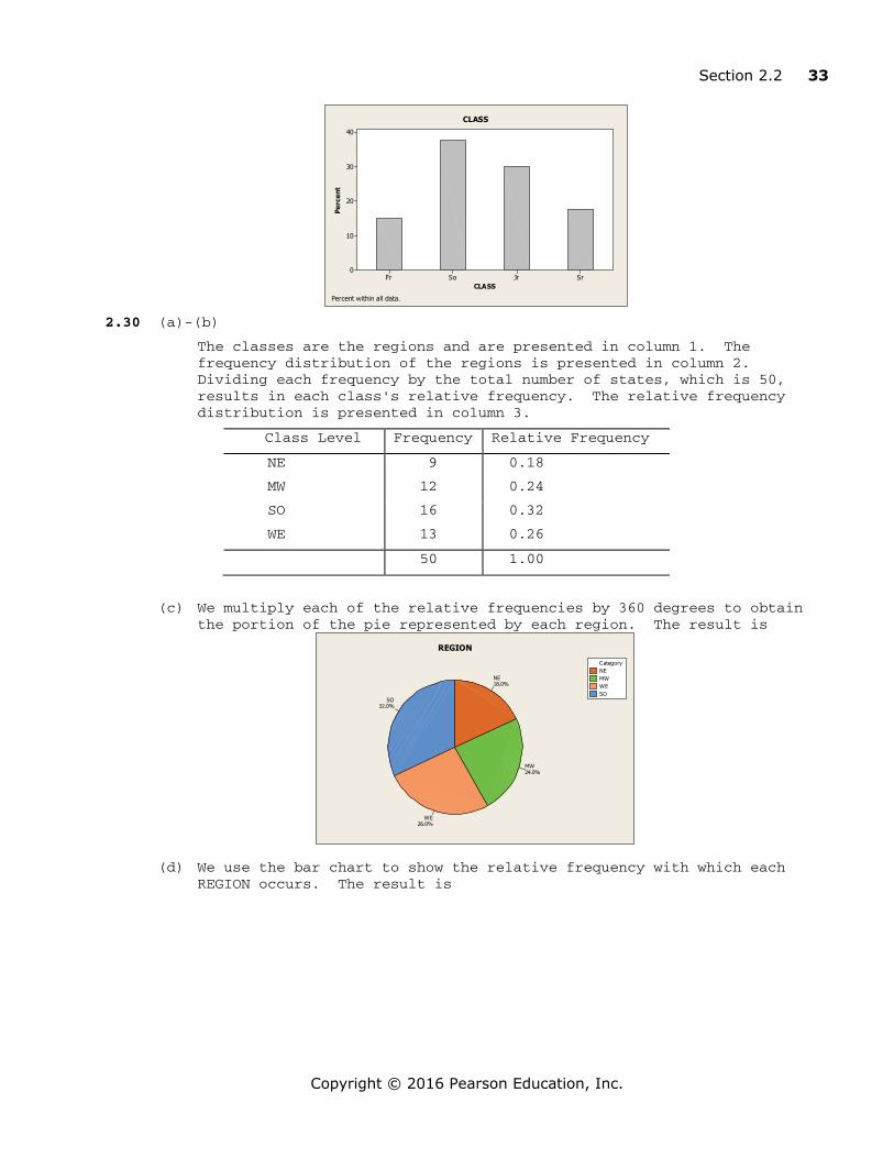
Section 2.2 33
Copyright © 2016 Pearson Education, Inc.
SrJrSoFr
40
30
20
10
0
CLASS
Perc
ent
CLASS
Percent within all data.
2.30 (a)-(b)
The classes are the regions and are presented in column 1. The frequency distribution of the regions is presented in column 2. Dividing each frequency by the total number of states, which is 50, results in each class's relative frequency. The relative frequency distribution is presented in column 3.
Class Level Frequency Relative Frequency NE 9 0.18
MW 12 0.24
SO 16 0.32
WE 13 0.26
50 1.00
(c) We multiply each of the relative frequencies by 360 degrees to obtain the portion of the pie represented by each region. The result is
NEMWWESO
Category
SO32.0%
WE26.0%
MW24.0%
NE18.0%
REGION
(d) We use the bar chart to show the relative frequency with which each REGION occurs. The result is
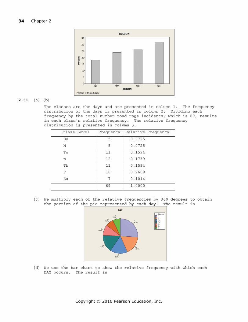
34 Chapter 2
Copyright © 2016 Pearson Education, Inc.
SOWEMWNE
35
30
25
20
15
10
5
0
REGION
Perc
ent
REGION
Percent within all data. 2.31 (a)-(b)
The classes are the days and are presented in column 1. The frequency distribution of the days is presented in column 2. Dividing each frequency by the total number road rage incidents, which is 69, results in each class's relative frequency. The relative frequency distribution is presented in column 3.
Class Level Frequency Relative Frequency
Su 5 0.0725
M 5 0.0725
Tu 11 0.1594
W 12 0.1739
Th 11 0.1594
F 18 0.2609
Sa 7 0.1014
69 1.0000
(c) We multiply each of the relative frequencies by 360 degrees to obtain the portion of the pie represented by each day. The result is
FWTuThSaSuM
CategoryM
7.2%Su
7.2%
Sa10.1%
Th15.9%
Tu15.9%
W17.4%
F26.1%
DAY
(d) We use the bar chart to show the relative frequency with which each DAY occurs. The result is

Section 2.2 35
Copyright © 2016 Pearson Education, Inc.
SaFThWTuMSu
25
20
15
10
5
0
DAY
Perc
ent
DAY
Percent within all data.
2.32 (a) We find each of the relative frequencies by dividing each of the frequencies by the total frequency of 291,176. Due to rounding, the sum of the relative frequency column is 0.9999.
Robbery Type Frequency Relative
Frequency Street/highway 127,403 0.4375
Commercial house 37,885 0.1301
Gas or service station 7,009 0.0241
Convenience store 14,863 0.0510
Residence 49,361 0.1695
Bank 5,777 0.0198
Miscellaneous 48,878 0.1679
291,176 0.9999
(b) We multiply each of the relative frequencies by 360 degrees to obtain
the portion of the pie represented by each robbery type. The result is
Street/highwayCommercial houseGas or service stationConvenience storeResidenceBankMiscellaneous
Category
Miscellaneous16.8%
Bank2.0%
Residence17.0%
Convenience store5.1%Gas or service station
2.4% Commercial house13.0%
Street/highway43.8%
Pie Chart of ROBBERY TYPE
(c) We use the bar chart to show the relative frequency with which each
robbery type occurs. The result is

36 Chapter 2
Copyright © 2016 Pearson Education, Inc.
Miscella
neous
Bank
Residenc
e
Convenien
ce sto
re
Gas or s
ervice
statio
n
Commercial
house
Stree
t/highw
ay
50
40
30
20
1 0
0
ROBBERY TYPEPe
rcen
t of F
REQU
ENCY
Percent within all data.
Bar Chart
2.33 (a) We find the relative frequencies by dividing each of the frequencies by
the total sample size of 509.
Color Frequency Relative Frequency
Brown 152 0.2986
Yellow 114 0.2240
Red 106 0.2083
Orange 51 0.1002
Green 43 0.0845
Blue 43 0.0845
509 1.0000
(b) We multiply each of the relative frequencies by 360 degrees to obtain
the portion of the pie represented by each color of M&M. The result is
0.0844794, 8.4%BLUE
0.0844794, 8.4%GREEN
0.100196, 10.0%ORANGE
0.208251, 20.8%RED
0.223969, 22.4%YELLOW
0.298625, 29.9%BROWN
Pie Chart of RELATIVE FREQUENCY vs COLOR

Section 2.2 37
Copyright © 2016 Pearson Education, Inc.
(c) We use the bar chart to show the relative frequency with which each color occurs. The result is
2.34 (a) We find the relative frequencies by dividing each of the frequencies by
the total sample size of 500.
Political View Frequency Relative Frequency
Liberal 147 0.294
Moderate 237 0.474
Conservative 116 0.232
500 1.000
(b) We multiply each of the relative frequencies by 360 degrees to obtain
the portion of the pie represented by each political view. The result is
LiberalModerateConservative
Category
Conservative23.2%
Moderate47.4%
Liberal29.4%
Pie Chart of VIEW
(c) We use the bar chart to show the relative frequency with which each
political view occurs. The result is
COLOR
RELA
TIVE
FRE
QUEN
CY
BLUEGREENORANGEREDYELLOWBROWN
0.30
0.25
0.20
0.15
0.10
0.05
0.00
Chart of RELATIVE FREQUENCY vs COLOR

38 Chapter 2
Copyright © 2016 Pearson Education, Inc.
ConservativeModerateLiberal
50
40
30
20
1 0
0
POLITICAL VIEWPe
rcen
t of F
REQU
ENCY
Percent within all data.
Bar Chart
2.35 (a) We find the relative frequencies by dividing each of the frequencies by the total sample size of 137,925.
Rank Frequency Relative
Frequency Professor 32,511 0.2357
Associate professor 28,572 0.2072
Assistant professor 59,277 0.4298
Instructor 14,289 0.1036
Other 3,276 0.0238
137,925 1.0000
(b) We multiply each of the relative frequencies by 360 degrees to obtain
the portion of the pie represented by each rank. The result is
ProfessorAssociate professorAssistant professorInstructorother
Categoryother2.4%Instructor
10.4%
Assistant professor43.0%
Associate professor20.7%
Professor23.6%
Pie Chart of RANK
(c) We use the bar chart to show the relative frequency with which each
rank occurs. The result is

Section 2.2 39
Copyright © 2016 Pearson Education, Inc.
OtherInstructorAssistant professorAssociate professorProfessor
40
30
20
1 0
0
RANKPe
rcen
t of F
REQU
ENCY
Percent within all data.
Bar Chart
2.36 (a) We find the relative frequencies by dividing each of the frequencies by the total sample size of 226. The sum of the relative frequency columns is 0.9999 due to rounding.
Drug Sold Frequency Relative
Frequency Marijuana 73 0.3230
Crack cocaine 62 0.2743
Powder cocaine 45 0.1991
Ecstasy 20 0.0885
Methamphetamine 17 0.0752
Heroin 5 0.0221
Other 4 0.0177
226 0.9999
(b) We multiply each of the relative frequencies by 360 degrees to obtain
the portion of the pie represented by each drug type. The result is
MarijuanaCrack cocainePowder cocaineEcstasyMethamphetamineHeroinother
Categoryother1.8%
Heroin2.2%Methamphetamine
7.5%
Ecstasy8.8%
Powder cocaine19.9%
Crack cocaine27.4%
Marijuana32.3%
Pie Chart of DRUG
(c) We use the bar chart to show the relative frequency with which each
rank occurs. The result is

40 Chapter 2
Copyright © 2016 Pearson Education, Inc.
Other
Heroin
Methamphe
tamine
Ecstas
y
Powder
cocaine
Crack cocai
ne
Marijua
na
35
30
25
20
15
10
5
0
DRUG
Perc
ent o
f FRE
QUEN
CY
Percent within all data.
Bar Chart
2.37 (a) We first find the relative frequencies by dividing each of the frequencies by the total sample size of 200.
Color Frequency Relative Frequency
Red 88 0.44
Black 102 0.51
Green 10 0.05
200 1.00
(b) We multiply each of the relative frequencies by 360 degrees to obtain
the portion of the pie represented by each color. The result is
BlackRedGreen
CategoryGreen5.0%
Red44.0%
Black51.0%
COLOR
(c) We use the bar chart to show the relative frequency with which each
color occurs. The result is

Section 2.2 41
Copyright © 2016 Pearson Education, Inc.
GreenBlackRed
50
40
30
20
10
0
NUMBER
Perc
ent
of F
REQU
ENCY
COLOR
Percent within all data.
2.38 (a) The classes are the different levels of health status and are presented in column 1. The frequency distribution of health status is presented in column 2. Dividing each frequency by the total number of people, which is 188.3 million for persons aged 19-64 and 41.5 million for persons aged 65 and over, results in each class's relative frequency. The relative frequency distribution is presented in column 3.
For People aged 19-64
Health Status Frequency Relative Frequency
Excellent or very good 119.7 0.636
Good 48.4 0.257
Fair or poor 20.2 0.107
188.3 1.000
For People aged 65 and over
Health Status Frequency Relative Frequency
Excellent or very good 18.1 0.436
Good 14.2 0.342
Fair or poor 9.2 0.222
41.5 1.000
(b) We multiply each of the relative frequencies by 360 degrees to obtain
the portion of each pie represented by each health status. The results are

42 Chapter 2
Copyright © 2016 Pearson Education, Inc.
1 9-64 65+Excellent /very goodGoodFair or poor
Category
Fair or poor10.7%
Good25.7%
Excellent /very good63.6%
Fair or poor22.2%
Good34.2%
Excellent /very good43.6%
Pie Chart of HEALTH STATUS
(c) A bigger proportion of persons aged 19-64 have a health status of
excellent or very good than persons aged 65 and over. A smaller proportion of persons aged 19-64 have a health status of fair or poor than persons aged 65 and over.
2.39 (a) Using Minitab, retrieve the data from the WeissStats Resource Site. Column 1 contains the type of the vehicle. From the tool bar, select
Stat < Tables < Tally Individual Variables, double-click on TYPE in the first box so that TYPE appears in the Variables box, put a check mark next to Counts and Percents under Display, and click OK. The result is
TYPE Count Percent Bus 21 2.80 Car 667 88.93
Truck 62 8.27 N= 750
(b) The relative frequencies were calculated in part(a) by putting a check
mark next to Percents. 2.8% of the vehicles were busses, 88.93% of the vehicles were cars, and 8.27% of the vehicles were trucks.
(c) Using Minitab, select Graph < Pie Chart, check Chart counts of unique values, double-click on TYPE in the first box so that TYPE appears in the Categorical Variables box. Click Pie Options, check decreasing volume, click OK. Click Labels, enter TYPE in for the title, click Slice Labels, check Category Name, Percent, and Draw a line from label to slice, Click OK twice. The result is
CarTruckBus
CategoryBus2.8%Truck
8.3%
Car88.9%
Pie Chart of TYPE

Section 2.2 43
Copyright © 2016 Pearson Education, Inc.
(d) Using Minitab, select Graph < Bar Chart, select Counts of unique values, select Simple option, click OK. Double-click on TYPE in the first box so that TYPE appears in the Categorical Variables box. Select Chart Options, check decreasing Y, check show Y as a percent, click OK. Select Labels, enter in TYPE as the title. Click OK twice. The result is
BusTruckCar
90
80
70
60
50
40
30
20
10
0
TYPE
Perc
ent
TYPE
Percent within all data.
2.40 (a) Using Minitab, retrieve the data from the WeissStats Resource Site. Column 2 contains the marital status and column 3 contains the number
of drinks per month. From the tool bar, select Stat < Tables < Tally Individual Variables, double-click on STATUS and DRINKS in the first box so that both STATUS and DRINKS appear in the Variables box, put a check mark next to Counts and Percents under Display, and click OK. The results are
STATUS Count Percent DRINKS Count Percent Single 354 19.98 Abstain 590 33.30 Married 1173 66.20 1-60 957 54.01 Widowed 143 8.07 Over 60 225 12.70 Divorced 102 5.76 N= 1772 N= 1772
(b) The relative frequencies were calculated in part(a) by putting a check
mark next to Percents. For the STATUS variable; 19.98% of the US Adults are single, 66.20% are married, 8.07% are widowed, and 5.76% are divorced. For the DRINKS variable, 33.30% of US Adults abstain from drinking, 54.01% have 1-60 drinks per month, and 12.70% have over 60 drinks per month.
(c) Using Minitab, select Graph < Pie Chart, check Chart counts of unique values, double-click on STATUS and DRINKS in the first box so that STATUS and DRINKS appear in the Categorical Variables box. Click Pie Options, check decreasing volume, click OK. Click Multiple Graphs, check On the Same Graphs, Click OK. Click Labels, click Slice Labels, check Category Name, Percent, and Draw a line from label to slice, Click OK twice. The results are
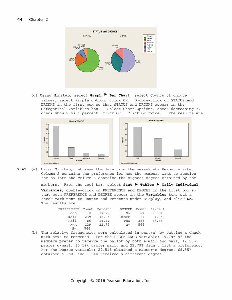
44 Chapter 2
Copyright © 2016 Pearson Education, Inc.
STATUS DRINKSMarriedSingleWidowedDivorcedAbstain1-60Over 60
Category
Divorced5.8%Widowed
8.1%
Single20.0%
Married66.2%
Over 6012.7%
Abstain33.3%
1-6054.0%
STATUS and DRINKS
(d) Using Minitab, select Graph < Bar Chart, select Counts of unique values, select Simple option, click OK. Double-click on STATUS and DRINKS in the first box so that STATUS and DRINKS appear in the Categorical Variables box. Select Chart Options, check decreasing Y, check show Y as a percent, click OK. Click OK twice. The results are
DivorcedWidowedSingleMarried
70
60
50
40
30
20
10
0
STATUS
Perc
ent
Chart of STATUS
Percent within all data.
Over 60Abstain1-60
60
50
40
30
20
10
0
DRINKS
Perc
ent
Chart of DRINKS
Percent within all data.
2.41 (a) Using Minitab, retrieve the data from the WeissStats Resource Site. Column 2 contains the preference for how the members want to receive the ballots and column 3 contains the highest degree obtained by the
members. From the tool bar, select Stat < Tables < Tally Individual Variables, double-click on PREFERENCE and DEGREE in the first box so that both PREFERENCE and DEGREE appear in the Variables box, put a check mark next to Counts and Percents under Display, and click OK. The results are
PREFERENCE Count Percent DEGREE Count Percent Both 112 19.79 MA 167 29.51 Email 239 42.23 Other 11 1.94 Mail 86 15.19 PhD 388 68.55 N/A 129 22.79 N= 566
N= 566 (b) The relative frequencies were calculated in part(a) by putting a check
mark next to Percents. For the PREFERENCE variable; 19.79% of the members prefer to receive the ballot by both e-mail and mail, 42.23% prefer e-mail, 15.19% prefer mail, and 22.79% didn’t list a preference. For the Degree variable; 29.51% obtained a Master’s degree, 68.55% obtained a PhD, and 1.94% received a different degree.
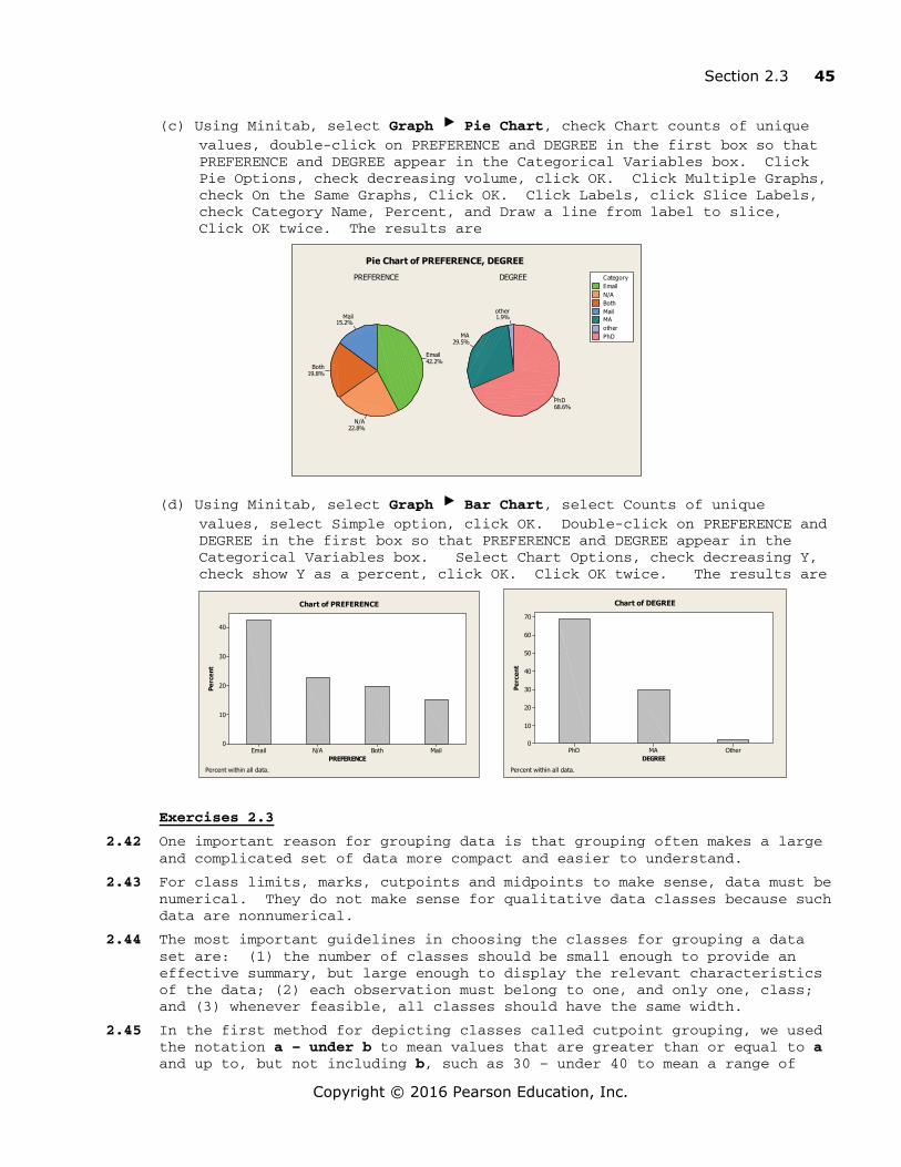
Section 2.3 45
Copyright © 2016 Pearson Education, Inc.
(c) Using Minitab, select Graph < Pie Chart, check Chart counts of unique values, double-click on PREFERENCE and DEGREE in the first box so that PREFERENCE and DEGREE appear in the Categorical Variables box. Click Pie Options, check decreasing volume, click OK. Click Multiple Graphs, check On the Same Graphs, Click OK. Click Labels, click Slice Labels, check Category Name, Percent, and Draw a line from label to slice, Click OK twice. The results are
PREFERENCE DEGREEEmailN/ABothMailMAotherPhD
Category
Mail15.2%
Both19.8%
N/A22.8%
Email42.2%
other1.9%
MA29.5%
PhD68.6%
Pie Chart of PREFERENCE, DEGREE
(d) Using Minitab, select Graph < Bar Chart, select Counts of unique values, select Simple option, click OK. Double-click on PREFERENCE and DEGREE in the first box so that PREFERENCE and DEGREE appear in the Categorical Variables box. Select Chart Options, check decreasing Y, check show Y as a percent, click OK. Click OK twice. The results are
MailBothN/AEmail
40
30
20
10
0
PREFERENCE
Perc
ent
Chart of PREFERENCE
Percent within all data.
OtherMAPhD
70
60
50
40
30
20
10
0
DEGREE
Perc
ent
Chart of DEGREE
Percent within all data.
Exercises 2.3
2.42 One important reason for grouping data is that grouping often makes a large and complicated set of data more compact and easier to understand.
2.43 For class limits, marks, cutpoints and midpoints to make sense, data must be numerical. They do not make sense for qualitative data classes because such data are nonnumerical.
2.44 The most important guidelines in choosing the classes for grouping a data set are: (1) the number of classes should be small enough to provide an effective summary, but large enough to display the relevant characteristics of the data; (2) each observation must belong to one, and only one, class; and (3) whenever feasible, all classes should have the same width.
2.45 In the first method for depicting classes called cutpoint grouping, we used the notation a – under b to mean values that are greater than or equal to a and up to, but not including b, such as 30 – under 40 to mean a range of

46 Chapter 2
Copyright © 2016 Pearson Education, Inc.
values greater than or equal to 30, but strictly less than 40. In the alternate method called limit grouping, we used the notation a-b to indicate a class that extends from a to b, including both. For example, 30-39 is a class that includes both 30 and 39. The alternate method is especially appropriate when all of the data values are integers. If the data include values like 39.7 or 39.93, the first method is more advantageous since the cutpoints remain integers; whereas, in the alternate method, the upper limits for each class would have to be expressed in decimal form such as 39.9 or 39.99.
2.46 (a) For continuous data displayed to one or more decimal places, using the cutpoint grouping is best since the description of the classes is simpler, regardless of the number of decimal places displayed.
(b) For discrete data with relatively few distinct observations, the single value grouping is best since either of the other two methods would result in combining some of those distinct values into single classes, resulting in too few classes, possibly less than 5.
2.47 For limit grouping, we find the class mark, which is the average of the lower and upper class limit. For cutpoint grouping, we find the class midpoint, which is the average of the two cutpoints.
2.48 A frequency histogram shows the actual frequencies on the vertical axis; whereas, the relative frequency histogram always shows proportions (between 0 and 1) or percentages (between 0 and 100) on the vertical axis.
2.49 An advantage of the frequency histogram over a frequency distribution is that it is possible to get an overall view of the data more easily. A disadvantage of the frequency histogram is that it may not be possible to determine exact frequencies for the classes when the number of observations is large.
2.50 By showing the lower class limits (or cutpoints) on the horizontal axis, the range of possible data values in each class is immediately known and the class mark (or midpoint) can be quickly determined. This is particularly helpful if it is not convenient to make all classes the same width. The use of the class mark (or midpoint) is appropriate when each class consists of a single value (which is, of course, also the midpoint). Use of the class marks (or midpoints) is not appropriate in other situations since it may be difficult to determine the location of the class limits (or cutpoints) from the values of the class marks (or midpoints), particularly if the class marks (or midpoints) are not evenly spaced. Class Marks (or midpoints) cannot be used if there is an open class.
2.51 If the classes consist of single values, stem-and-leaf diagrams and frequency histograms are equally useful. If only one diagram is needed and the classes consist of more than one value, the stem-and-leaf diagram allows one to retrieve all of the original data values whereas the frequency histogram does not. If two or more sets of data of different sizes are to be compared, the relative frequency histogram is advantageous because all of the diagrams to be compared will have the same total relative frequency of 1.00. Finally, stem-and-leaf diagrams are not very useful with very large data sets and may present problems with data having many digits in each number.
2.52 The histogram (especially one using relative frequencies) is generally preferable. Data sets with a large number of observations may result in a stem of the stem-and-leaf diagram having more leaves than will fit on the line. In that case, the histogram would be preferable.

Section 2.3 47
Copyright © 2016 Pearson Education, Inc.
2.53 You can reconstruct the stem-and-leaf diagram using two lines per stem. For example, instead of listing all of the values from 10 to 19 on a ‘1’ stem, you can make two ‘1’ stems. On the first, you record the values from 10 to 14 and on the second, the values from 15 to 19. If there are still two few stems, you can reconstruct the diagram using five lines per stem, recording 10 and 11 on the first line, 12 and 13 on the second, and so on.
2.54 For the number of bedrooms per single-family dwelling, single-value grouping is probably the best because the data is discrete with relatively few distinct observations.
2.55 For the ages of householders, given as a whole number, limit grouping is probably the best because the data are given as whole numbers and there are probably too many distinct observations to list them as single-value grouping.
2.56 For additional sleep obtained by a sample of 100 patients by using a particular brand of sleeping pill, cutpoint grouping is probably the best because the data is continuous and the data was recorded to the nearest tenth of an hour.
2.57 For the number of automobiles per family, single-value grouping is probably the best because the data is discrete with relatively few distinct observations.
2.58 For gas mileages, rounded to the nearest number of miles per gallon, limit grouping is probably the best because the data are given as whole numbers and there are probably too many distinct observations to list them as single-value grouping.
2.59 For carapace length for a sample of giant tarantulas, cutpoint grouping is probably the best because the data is continuous and the data was recorded to the nearest hundredth of a millimeter.
2.60 (a) Since the data values range from 1 to 4, we construct a table with classes based on a single value. The resulting table follows.
Single Value Class Frequency 1 2 2 0 3 5 4 3 10
(b) To get the relative frequencies, divide each frequency by the sample size of 10.
Single Value Class Relative Frequency 1 0.20 2 0.00 3 0.50 4 0.30 1.00
(c) The frequency histogram in Figure (a) is constructed using the frequency distribution presented in part (a) of this exercise. Column 1 demonstrates that the data are grouped using classes based on a single value. These single values in column 1 are used to label the horizontal axis of the frequency histogram. When classes are based on a single value, the middle of each histogram bar is placed directly over the single numerical value represented by the class. Also, the height of each bar in the frequency histogram matches the respective frequency in column 2.

48 Chapter 2
Copyright © 2016 Pearson Education, Inc.
Figure (a) Figure (b)
4321
5
4
3
2
1
0
DATA
Freq
uenc
y
4321
50
40
30
20
1 0
0
DATA
Perc
ent
(d) The relative-frequency histogram in Figure (b) is constructed using the relative-frequency distribution presented in part (b) of this exercise. It has the same horizontal axis as the frequency histogram. The middle of each histogram bar is placed directly over the single numerical value represented by the class. Also, the height of each bar in the relative-frequency histogram matches the respective relative frequency in column 2.
2.61 (a) Since the data values range from 1 to 4, we construct a table with classes based on a single value. The resulting table follows.
Single Value Class Frequency 1 2 2 2 3 5 4 1 10
(b) To get the relative frequencies, divide each frequency by the sample size of 10.
Single Value Class Relative Frequency 1 0.20 2 0.20 3 0.50 4 0.10 1.00
(c) The frequency histogram in Figure (a) is constructed using the frequency distribution presented in part (a) of this exercise. Column 1 demonstrates that the data are grouped using classes based on a single value. These single values in column 1 are used to label the horizontal axis of the frequency histogram. When classes are based on a single value, the middle of each histogram bar is placed directly over the single numerical value represented by the class. Also, the height of each bar in the frequency histogram matches the respective frequency in column 2.

Section 2.3 49
Copyright © 2016 Pearson Education, Inc.
Figure (a) Figure (b)
4321
5
4
3
2
1
0
DATA
Freq
uenc
y
4321
50
40
30
20
1 0
0
DATA
Perc
ent
(d) The relative-frequency histogram in Figure (b) is constructed using the relative-frequency distribution presented in part (b) of this exercise. It has the same horizontal axis as the frequency histogram. The middle of each histogram bar is placed directly over the single numerical value represented by the class. Also, the height of each bar in the relative-frequency histogram matches the respective relative frequency in column 2.
2.62 (a) Since the data values range from 0 to 4, we construct a table with classes based on a single value. The resulting table follows.
Single Value Class Frequency 0 2 1 8 2 7 3 2 4 1 20
(b) To get the relative frequencies, divide each frequency by the sample size of 20.
Single Value Class Relative Frequency 0 0.10 1 0.40 2 0.35 3 0.10 4 0.05 1.00
(c) The frequency histogram in Figure (a) is constructed using the frequency distribution presented in part (a) of this exercise. Column 1 demonstrates that the data are grouped using classes based on a single value. These single values in column 1 are used to label the horizontal axis of the frequency histogram. When classes are based on a single value, the middle of each histogram bar is placed directly over the single numerical value represented by the class. Also, the height of each bar in the frequency histogram matches the respective frequency in column 2.
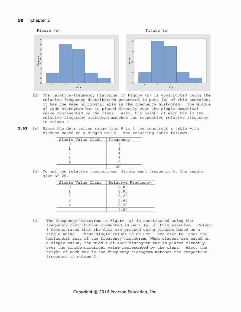
50 Chapter 2
Copyright © 2016 Pearson Education, Inc.
Figure (a) Figure (b)
43210
9
8
7
6
5
4
3
2
1
0
DATA
Freq
uenc
y
43210
40
30
20
1 0
0
DATA
Perc
ent
(d) The relative-frequency histogram in Figure (b) is constructed using the relative-frequency distribution presented in part (b) of this exercise. It has the same horizontal axis as the frequency histogram. The middle of each histogram bar is placed directly over the single numerical value represented by the class. Also, the height of each bar in the relative-frequency histogram matches the respective relative frequency in column 2.
2.63 (a) Since the data values range from 0 to 4, we construct a table with classes based on a single value. The resulting table follows.
Single Value Class Frequency 0 1 1 1 2 4 3 8 4 6 20
(b) To get the relative frequencies, divide each frequency by the sample size of 20.
Single Value Class Relative Frequency 0 0.05 1 0.05 2 0.20 3 0.40 4 0.30 1.00
(c) The frequency histogram in Figure (a) is constructed using the frequency distribution presented in part (a) of this exercise. Column 1 demonstrates that the data are grouped using classes based on a single value. These single values in column 1 are used to label the horizontal axis of the frequency histogram. When classes are based on a single value, the middle of each histogram bar is placed directly over the single numerical value represented by the class. Also, the height of each bar in the frequency histogram matches the respective frequency in column 2.
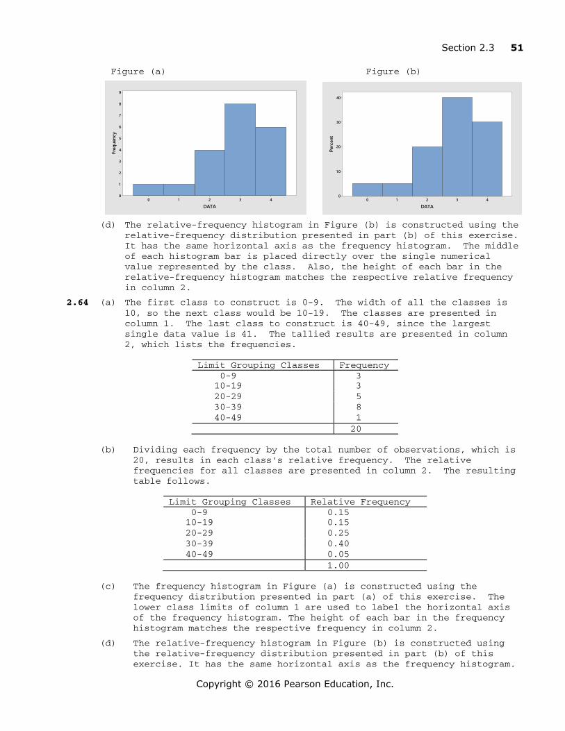
Section 2.3 51
Copyright © 2016 Pearson Education, Inc.
Figure (a) Figure (b)
43210
9
8
7
6
5
4
3
2
1
0
DATA
Freq
uenc
y
43210
40
30
20
1 0
0
DATA
Perc
ent
(d) The relative-frequency histogram in Figure (b) is constructed using the relative-frequency distribution presented in part (b) of this exercise. It has the same horizontal axis as the frequency histogram. The middle of each histogram bar is placed directly over the single numerical value represented by the class. Also, the height of each bar in the relative-frequency histogram matches the respective relative frequency in column 2.
2.64 (a) The first class to construct is 0-9. The width of all the classes is 10, so the next class would be 10-19. The classes are presented in column 1. The last class to construct is 40-49, since the largest single data value is 41. The tallied results are presented in column 2, which lists the frequencies.
(b) Dividing each frequency by the total number of observations, which is 20, results in each class's relative frequency. The relative frequencies for all classes are presented in column 2. The resulting table follows.
(c) The frequency histogram in Figure (a) is constructed using the frequency distribution presented in part (a) of this exercise. The lower class limits of column 1 are used to label the horizontal axis of the frequency histogram. The height of each bar in the frequency histogram matches the respective frequency in column 2.
(d) The relative-frequency histogram in Figure (b) is constructed using the relative-frequency distribution presented in part (b) of this exercise. It has the same horizontal axis as the frequency histogram.
Limit Grouping Classes Frequency 0-9 3 10-19 3 20-29 5 30-39 8 40-49 1 20
Limit Grouping Classes Relative Frequency 0-9 0.15 10-19 0.15 20-29 0.25 30-39 0.40 40-49 0.05 1.00

52 Chapter 2
Copyright © 2016 Pearson Education, Inc.
The height of each bar in the relative-frequency histogram matches the respective relative frequency in column 2.
Figure (a) Figure (b)
504030201 00
9
8
7
6
5
4
3
2
1
0
DATA
Freq
uenc
y
504030201 00
40
30
20
1 0
0
DATA
Perc
ent
2.65 (a) The first class to construct is 0-4. The width of all the classes is 5, so the next class would be 5-9. The classes are presented in column 1. The last class to construct is 25-29, since the largest single data value is 26. The tallied results are presented in column 2, which lists the frequencies.
(b) Dividing each frequency by the total number of observations, which is 20, results in each class's relative frequency. The relative frequencies for all classes are presented in column 2. The resulting table follows.
(c) The frequency histogram in Figure (a) is constructed using the frequency distribution presented in part (a) of this exercise. The lower class limits of column 1 are used to label the horizontal axis of the frequency histogram. The height of each bar in the frequency histogram matches the respective frequency in column 2.
(d) The relative-frequency histogram in Figure (b) is constructed using the relative-frequency distribution presented in part (b) of this exercise. It has the same horizontal axis as the frequency histogram. The height of each bar in the relative-frequency histogram matches the respective relative frequency in column 2.
Limit Grouping Classes Frequency 0-4 5 5-9 5 10-14 1 15-19 4 20-24 2 25-29 3 20
Limit Grouping Classes Relative Frequency 0-4 0.25 5-9 0.25 10-14 0.05 15-19 0.20 20-24 0.10 25-29 0.15 1.00
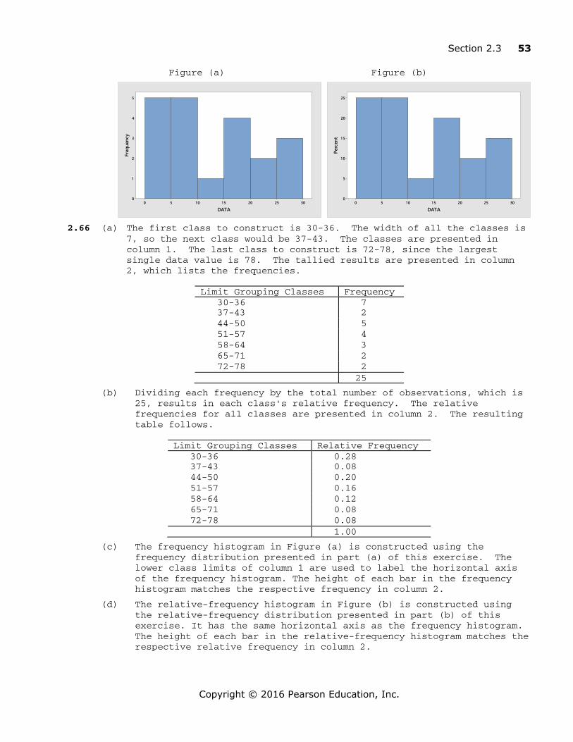
Section 2.3 53
Copyright © 2016 Pearson Education, Inc.
Figure (a) Figure (b)
3025201 51 050
5
4
3
2
1
0
DATA
Freq
uenc
y
3025201 51 050
25
20
1 5
1 0
5
0
DATA
Perc
ent
2.66 (a) The first class to construct is 30-36. The width of all the classes is 7, so the next class would be 37-43. The classes are presented in column 1. The last class to construct is 72-78, since the largest single data value is 78. The tallied results are presented in column 2, which lists the frequencies.
(b) Dividing each frequency by the total number of observations, which is 25, results in each class's relative frequency. The relative frequencies for all classes are presented in column 2. The resulting table follows.
(c) The frequency histogram in Figure (a) is constructed using the frequency distribution presented in part (a) of this exercise. The lower class limits of column 1 are used to label the horizontal axis of the frequency histogram. The height of each bar in the frequency histogram matches the respective frequency in column 2.
(d) The relative-frequency histogram in Figure (b) is constructed using the relative-frequency distribution presented in part (b) of this exercise. It has the same horizontal axis as the frequency histogram. The height of each bar in the relative-frequency histogram matches the respective relative frequency in column 2.
Limit Grouping Classes Frequency 30-36 7 37-43 2 44-50 5 51-57 4 58-64 3 65-71 2 72-78 2 25
Limit Grouping Classes Relative Frequency 30-36 0.28 37-43 0.08 44-50 0.20 51-57 0.16 58-64 0.12 65-71 0.08 72-78 0.08 1.00

54 Chapter 2
Copyright © 2016 Pearson Education, Inc.
Figure (a) Figure (b)
7872655851443730
7
6
5
4
3
2
1
0
DATA
Freq
uenc
y
7872655851443730
30
25
20
1 5
1 0
5
0
DATA
Perc
ent
2.67 (a) The first class to construct is 50-59. The width of all the classes is 10, so the next class would be 60-69. The classes are presented in column 1. The last class to construct is 90-99, since the largest single data value is 98. The tallied results are presented in column 2, which lists the frequencies.
(b) Dividing each frequency by the total number of observations, which is 25, results in each class's relative frequency. The relative frequencies for all classes are presented in column 2. The resulting table follows.
(c) The frequency histogram in Figure (a) is constructed using the frequency distribution presented in part (a) of this exercise. The lower class limits of column 1 are used to label the horizontal axis of the frequency histogram. The height of each bar in the frequency histogram matches the respective frequency in column 2.
(d) The relative-frequency histogram in Figure (b) is constructed using the relative-frequency distribution presented in part (b) of this exercise. It has the same horizontal axis as the frequency histogram. The height of each bar in the relative-frequency histogram matches the respective relative frequency in column 2.
Limit Grouping Classes Frequency 50-59 6 60-69 3 70-79 6 80-89 7 90-99 3 25
Limit Grouping Classes Relative Frequency 50-59 0.24 60-69 0.12 70-79 0.24 80-89 0.28 90-99 0.12 1.00

Section 2.3 55
Copyright © 2016 Pearson Education, Inc.
Figure (a) Figure (b)
1 009080706050
7
6
5
4
3
2
1
0
DATA
Freq
uenc
y
1 009080706050
30
25
20
1 5
1 0
5
0
DATA
Perc
ent
2.68 (a) The first class to construct is 10 – under 15. Since all classes are to be of equal width 5, the second class is 15 – under 20. All of the classes are presented in column 1. The last class to construct is 35 – under 40, since the largest single data value is 38.8. The results of the tallying are presented in column 2, which lists the frequencies.
Cutpoint Grouping Classes Frequency 10 – under 15 4 15 – under 20 5 20 – under 25 7 25 – under 30 3 30 – under 35 0 35 – under 40 1 20
(b) Dividing each frequency by the total number of observations, which is 20, results in each class's relative frequency. The relative frequencies for all classes are presented in column 2.
Cutpoint Grouping Classes Relative Frequency 10 – under 15 0.20 15 – under 20 0.25 20 – under 25 0.35 25 – under 30 0.15 30 – under 35 0.00 35 – under 40 0.05 1.00
(c) The frequency histogram in Figure (a) is constructed using the frequency distribution obtained in part (a) of this exercise. The cutpoints are used to label the horizontal axis. Also, the height of each bar in the frequency histogram matches the respective frequency in column 2.
(d) The relative-frequency histogram in Figure (b) is constructed using the relative-frequency distribution obtained in part (b) of this exercise. It has the same horizontal axis as the frequency histogram. The height of each bar in the relative-frequency histogram matches the respective relative frequency in column 2.
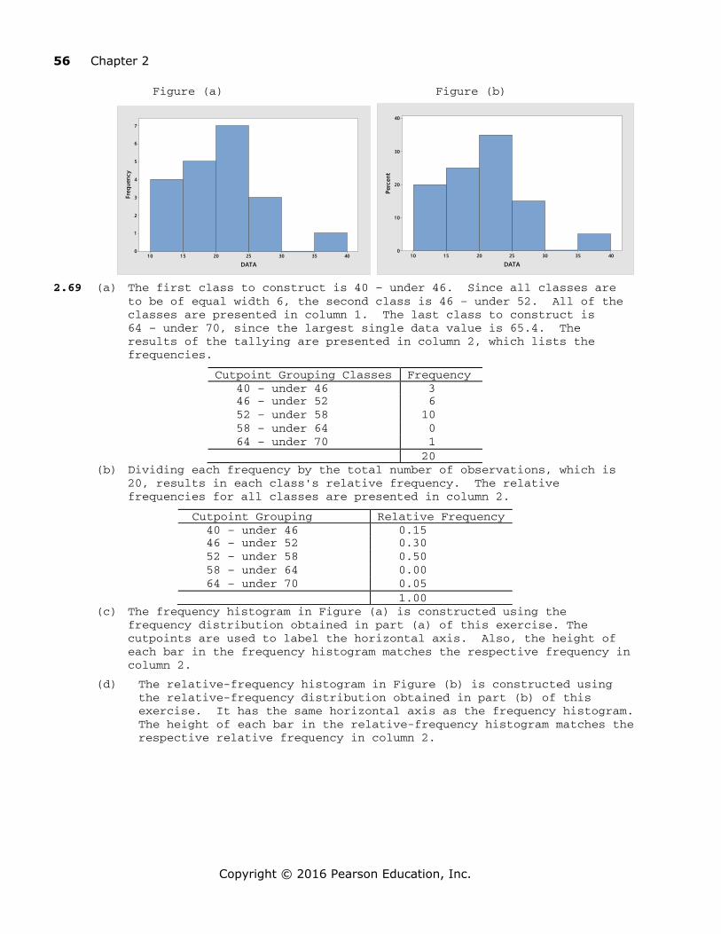
56 Chapter 2
Copyright © 2016 Pearson Education, Inc.
Figure (a) Figure (b)
40353025201 51 0
7
6
5
4
3
2
1
0
DATA
Freq
uenc
y
4035302520151 0
40
30
20
1 0
0
DATA
Perc
ent
2.69 (a) The first class to construct is 40 – under 46. Since all classes are to be of equal width 6, the second class is 46 – under 52. All of the classes are presented in column 1. The last class to construct is 64 – under 70, since the largest single data value is 65.4. The results of the tallying are presented in column 2, which lists the frequencies.
Cutpoint Grouping Classes Frequency 40 – under 46 3 46 – under 52 6 52 – under 58 10 58 – under 64 0 64 – under 70 1 20
(b) Dividing each frequency by the total number of observations, which is 20, results in each class's relative frequency. The relative frequencies for all classes are presented in column 2.
Cutpoint Grouping Relative Frequency 40 – under 46 0.15 46 – under 52 0.30 52 – under 58 0.50 58 – under 64 0.00 64 – under 70 0.05 1.00
(c) The frequency histogram in Figure (a) is constructed using the frequency distribution obtained in part (a) of this exercise. The cutpoints are used to label the horizontal axis. Also, the height of each bar in the frequency histogram matches the respective frequency in column 2.
(d) The relative-frequency histogram in Figure (b) is constructed using the relative-frequency distribution obtained in part (b) of this exercise. It has the same horizontal axis as the frequency histogram. The height of each bar in the relative-frequency histogram matches the respective relative frequency in column 2.
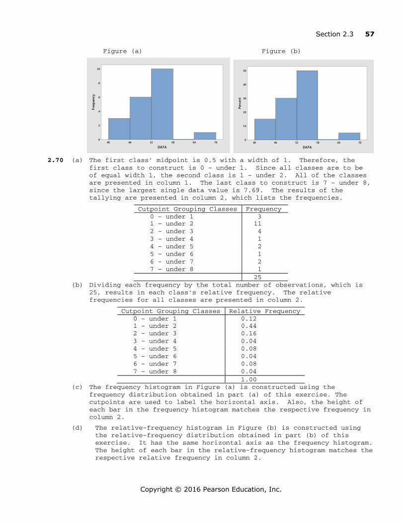
Section 2.3 57
Copyright © 2016 Pearson Education, Inc.
Figure (a) Figure (b)
706458524640
1 0
8
6
4
2
0
DATA
Freq
uenc
y
706458524640
50
40
30
20
1 0
0
DATA
Perc
ent
2.70 (a) The first class’ midpoint is 0.5 with a width of 1. Therefore, the first class to construct is 0 – under 1. Since all classes are to be of equal width 1, the second class is 1 – under 2. All of the classes are presented in column 1. The last class to construct is 7 – under 8, since the largest single data value is 7.69. The results of the tallying are presented in column 2, which lists the frequencies.
Cutpoint Grouping Classes Frequency 0 – under 1 3 1 – under 2 11 2 – under 3 4 3 – under 4 1 4 – under 5 2 5 – under 6 1 6 – under 7 2 7 – under 8 1 25
(b) Dividing each frequency by the total number of observations, which is 25, results in each class's relative frequency. The relative frequencies for all classes are presented in column 2.
Cutpoint Grouping Classes Relative Frequency 0 – under 1 0.12 1 – under 2 0.44 2 – under 3 0.16 3 – under 4 0.04 4 – under 5 0.08 5 – under 6 0.04 6 – under 7 0.08 7 – under 8 0.04
1.00 (c) The frequency histogram in Figure (a) is constructed using the
frequency distribution obtained in part (a) of this exercise. The cutpoints are used to label the horizontal axis. Also, the height of each bar in the frequency histogram matches the respective frequency in column 2.
(d) The relative-frequency histogram in Figure (b) is constructed using the relative-frequency distribution obtained in part (b) of this exercise. It has the same horizontal axis as the frequency histogram. The height of each bar in the relative-frequency histogram matches the respective relative frequency in column 2.
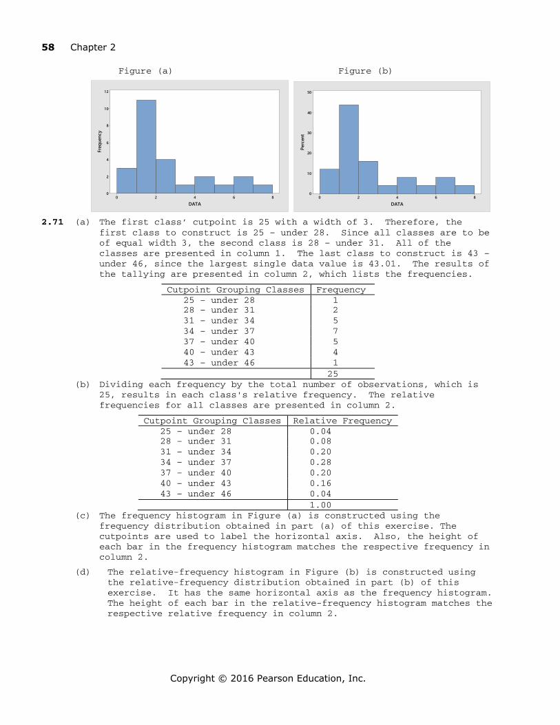
58 Chapter 2
Copyright © 2016 Pearson Education, Inc.
Figure (a) Figure (b)
86420
1 2
1 0
8
6
4
2
0
DATA
Freq
uenc
y
86420
50
40
30
20
1 0
0
DATA
Perc
ent
2.71 (a) The first class’ cutpoint is 25 with a width of 3. Therefore, the first class to construct is 25 – under 28. Since all classes are to be of equal width 3, the second class is 28 – under 31. All of the classes are presented in column 1. The last class to construct is 43 – under 46, since the largest single data value is 43.01. The results of the tallying are presented in column 2, which lists the frequencies.
Cutpoint Grouping Classes Frequency 25 – under 28 1 28 – under 31 2 31 – under 34 5 34 – under 37 7 37 – under 40 5 40 – under 43 4 43 – under 46 1 25
(b) Dividing each frequency by the total number of observations, which is 25, results in each class's relative frequency. The relative frequencies for all classes are presented in column 2.
Cutpoint Grouping Classes Relative Frequency 25 – under 28 0.04 28 – under 31 0.08 31 – under 34 0.20 34 – under 37 0.28 37 – under 40 0.20 40 – under 43 0.16 43 – under 46 0.04 1.00
(c) The frequency histogram in Figure (a) is constructed using the frequency distribution obtained in part (a) of this exercise. The cutpoints are used to label the horizontal axis. Also, the height of each bar in the frequency histogram matches the respective frequency in column 2.
(d) The relative-frequency histogram in Figure (b) is constructed using the relative-frequency distribution obtained in part (b) of this exercise. It has the same horizontal axis as the frequency histogram. The height of each bar in the relative-frequency histogram matches the respective relative frequency in column 2.

Section 2.3 59
Copyright © 2016 Pearson Education, Inc.
Figure (a) Figure (b)
4643403734312825
7
6
5
4
3
2
1
0
DATA
Freq
uenc
y
4643403734312825
30
25
20
1 5
1 0
5
0
DATA
Perc
ent
2.72 The horizontal axis of this dotplot displays a range of possible values. To complete the dotplot, we go through the data set and record data value by placing a dot over the appropriate value on the horizontal axis.
4321DATA
Dotplot of DATA
2.73 The horizontal axis of this dotplot displays a range of possible values. To complete the dotplot, we go through the data set and record data value by placing a dot over the appropriate value on the horizontal axis.
3210DATA
Dotplot of DATA
2.74 The horizontal axis of this dotplot displays a range of possible values. To complete the dotplot, we go through the data set and record data value by placing a dot over the appropriate value on the horizontal axis.
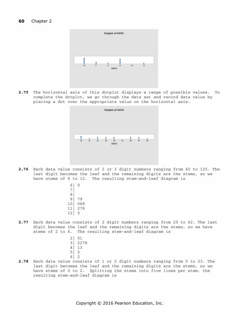
60 Chapter 2
Copyright © 2016 Pearson Education, Inc.
1 51 41 31 21 11 0DATA
Dotplot of DATA
2.75 The horizontal axis of this dotplot displays a range of possible values. To complete the dotplot, we go through the data set and record data value by placing a dot over the appropriate value on the horizontal axis.
383736353433323130DATA
Dotplot of DATA
2.76 Each data value consists of 2 or 3 digit numbers ranging from 60 to 125. The last digit becomes the leaf and the remaining digits are the stems, so we have stems of 6 to 12. The resulting stem-and-leaf diagram is
6| 0 7|
8| 9| 79
10| 068 11| 278 12| 5
2.77 Each data value consists of 2 digit numbers ranging from 20 to 62. The last
digit becomes the leaf and the remaining digits are the stems, so we have stems of 2 to 6. The resulting stem-and-leaf diagram is
2| 01 3| 2278
4| 13 5| 5
6| 2 2.78 Each data value consists of 1 or 2 digit numbers ranging from 5 to 23. The
last digit becomes the leaf and the remaining digits are the stems, so we have stems of 0 to 2. Splitting the stems into five lines per stem, the resulting stem-and-leaf diagram is
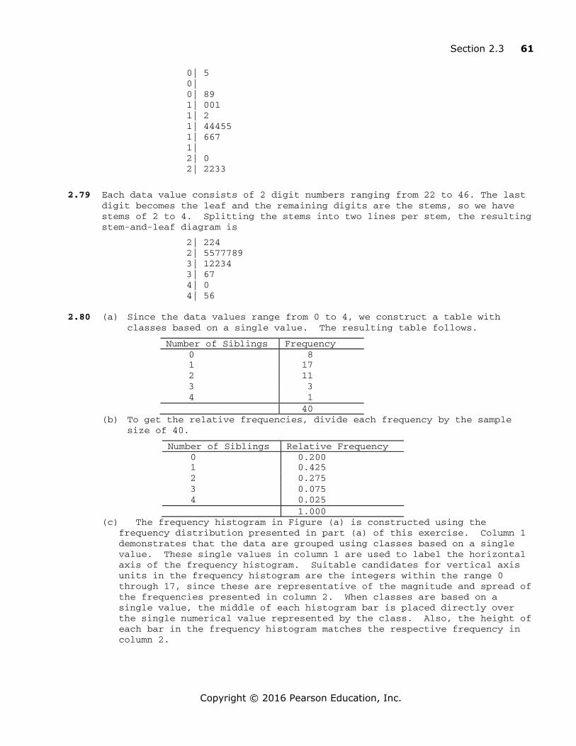
Section 2.3 61
Copyright © 2016 Pearson Education, Inc.
0| 5 0| 0| 89
1| 001 1| 2
1| 44455 1| 667 1|
2| 0 2| 2233
2.79 Each data value consists of 2 digit numbers ranging from 22 to 46. The last digit becomes the leaf and the remaining digits are the stems, so we have stems of 2 to 4. Splitting the stems into two lines per stem, the resulting stem-and-leaf diagram is
2| 224 2| 5577789 3| 12234
3| 67 4| 0
4| 56 2.80 (a) Since the data values range from 0 to 4, we construct a table with
classes based on a single value. The resulting table follows.
Number of Siblings Frequency 0 8 1 17 2 11 3 3 4 1 40
(b) To get the relative frequencies, divide each frequency by the sample size of 40.
Number of Siblings Relative Frequency 0 0.200 1 0.425 2 0.275 3 0.075 4 0.025 1.000
(c) The frequency histogram in Figure (a) is constructed using the frequency distribution presented in part (a) of this exercise. Column 1 demonstrates that the data are grouped using classes based on a single value. These single values in column 1 are used to label the horizontal axis of the frequency histogram. Suitable candidates for vertical axis units in the frequency histogram are the integers within the range 0 through 17, since these are representative of the magnitude and spread of the frequencies presented in column 2. When classes are based on a single value, the middle of each histogram bar is placed directly over the single numerical value represented by the class. Also, the height of each bar in the frequency histogram matches the respective frequency in column 2.

62 Chapter 2
Copyright © 2016 Pearson Education, Inc.
SIBLINGS
Freq
uenc
y
43210
18
16
14
12
10
8
6
4
2
0
Histogram of SIBLINGS
SIBLINGS
Perc
ent
43210
40
30
20
10
0
Histogram of SIBLINGS
Figure (a) Figure (b)
(d) The relative-frequency histogram in Figure (b) is constructed using the relative-frequency distribution presented in part (b) of this exercise. It has the same horizontal axis as the frequency histogram. We notice that the relative frequencies presented in column 2 range in size from 0.025 to 0.425. Thus, suitable candidates for vertical-axis units in the relative-frequency histogram are increments of 0.05 (or 5%), from zero to 0.45 (or 45%). The middle of each histogram bar is placed directly over the single numerical value represented by the class. Also, the height of each bar in the relative-frequency histogram matches the respective relative frequency in column 2.
2.81 (a) Since the data values range from 1 to 7, we construct a table with classes based on a single value. The resulting table follows.
Number of Persons Frequency
1 7
2 13
3 9
4 5
5 4
6 1
7 1
40
(b) To get the relative frequencies, divide each frequency by the sample size of 40.
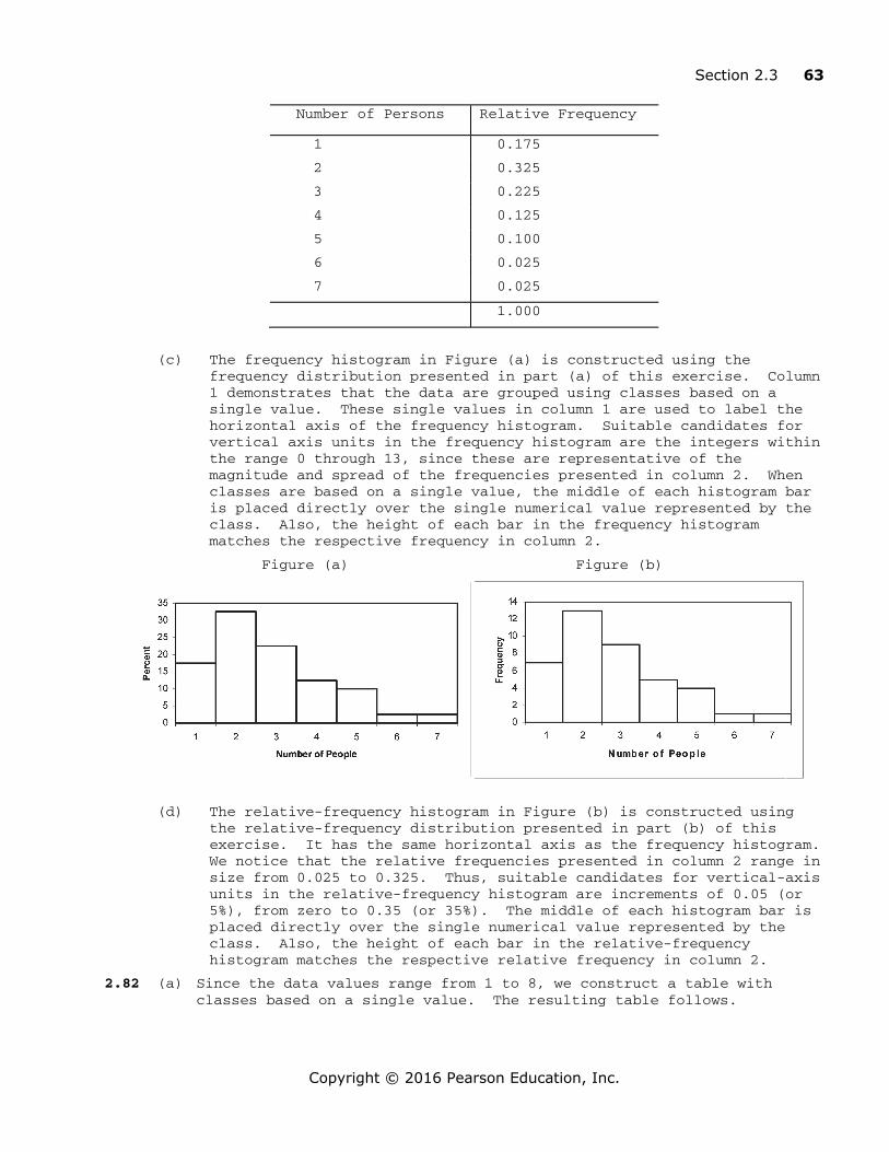
Section 2.3 63
Copyright © 2016 Pearson Education, Inc.
Number of Persons Relative Frequency
1 0.175
2 0.325
3 0.225
4 0.125
5 0.100
6 0.025
7 0.025
1.000
(c) The frequency histogram in Figure (a) is constructed using the frequency distribution presented in part (a) of this exercise. Column 1 demonstrates that the data are grouped using classes based on a single value. These single values in column 1 are used to label the horizontal axis of the frequency histogram. Suitable candidates for vertical axis units in the frequency histogram are the integers within the range 0 through 13, since these are representative of the magnitude and spread of the frequencies presented in column 2. When classes are based on a single value, the middle of each histogram bar is placed directly over the single numerical value represented by the class. Also, the height of each bar in the frequency histogram matches the respective frequency in column 2.
Figure (a) Figure (b)
(d) The relative-frequency histogram in Figure (b) is constructed using the relative-frequency distribution presented in part (b) of this exercise. It has the same horizontal axis as the frequency histogram. We notice that the relative frequencies presented in column 2 range in size from 0.025 to 0.325. Thus, suitable candidates for vertical-axis units in the relative-frequency histogram are increments of 0.05 (or 5%), from zero to 0.35 (or 35%). The middle of each histogram bar is placed directly over the single numerical value represented by the class. Also, the height of each bar in the relative-frequency histogram matches the respective relative frequency in column 2.
2.82 (a) Since the data values range from 1 to 8, we construct a table with classes based on a single value. The resulting table follows.
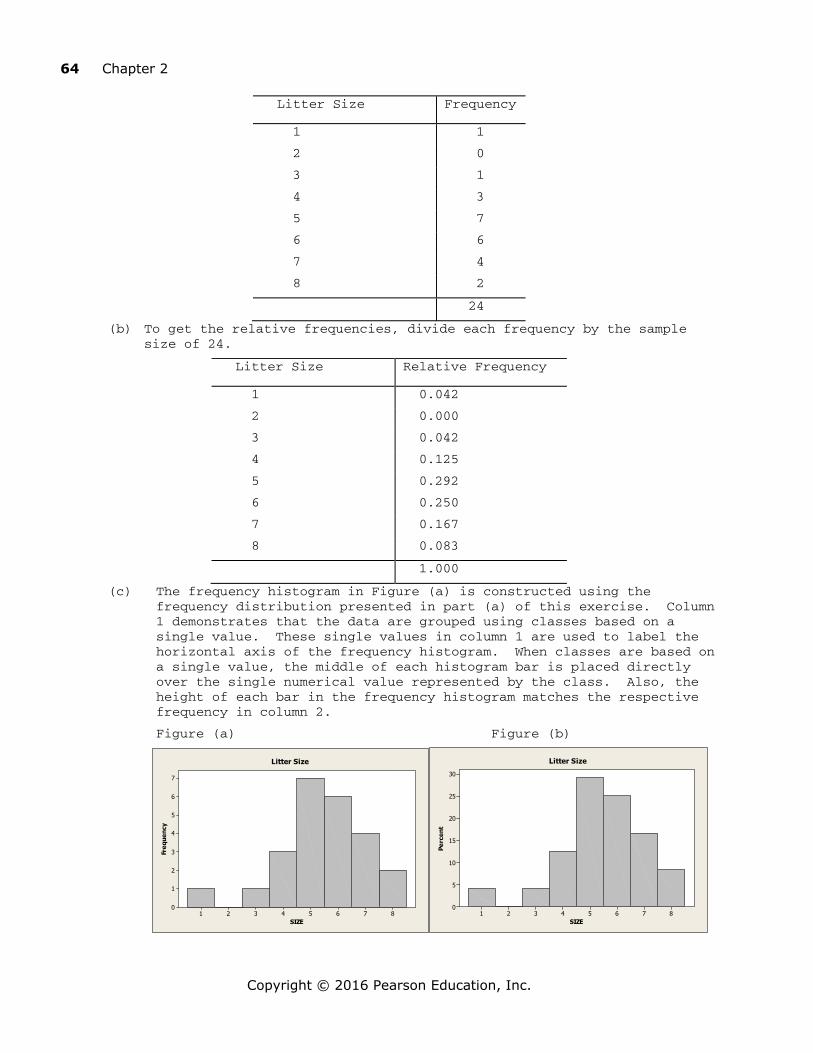
64 Chapter 2
Copyright © 2016 Pearson Education, Inc.
Litter Size Frequency
1 1
2 0
3 1
4 3
5 7
6 6
7 4
8 2
24
(b) To get the relative frequencies, divide each frequency by the sample size of 24.
Litter Size Relative Frequency
1 0.042
2 0.000
3 0.042
4 0.125
5 0.292
6 0.250
7 0.167
8 0.083
1.000
(c) The frequency histogram in Figure (a) is constructed using the frequency distribution presented in part (a) of this exercise. Column 1 demonstrates that the data are grouped using classes based on a single value. These single values in column 1 are used to label the horizontal axis of the frequency histogram. When classes are based on a single value, the middle of each histogram bar is placed directly over the single numerical value represented by the class. Also, the height of each bar in the frequency histogram matches the respective frequency in column 2.
Figure (a) Figure (b)
87654321
7
6
5
4
3
2
1
0
SIZE
Freq
uenc
y
Litter Size
87654321
30
25
20
15
10
5
0
SIZE
Perc
ent
Litter Size

Section 2.3 65
Copyright © 2016 Pearson Education, Inc.
(d) The relative-frequency histogram in Figure (b) is constructed using the relative-frequency distribution presented in part (b) of this exercise. It has the same horizontal axis as the frequency histogram. We notice that the relative frequencies presented in column 2 range in size from 0.000 to 0.292. Thus, suitable candidates for vertical-axis units in the relative-frequency histogram are increments of 0.05 (or 5%), from zero to 0.30 (or 30%). The middle of each histogram bar is placed directly over the single numerical value represented by the class. Also, the height of each bar in the relative-frequency histogram matches the respective relative frequency in column 2.
2.83 (a) Since the data values range from 0 to 5, we construct a table with classes based on a single value. The resulting table follows.
Number of Computers Frequency 0 5 1 22 2 11 3 2 4 4 5 1 45
(b) To get the relative frequencies, divide each frequency by the sample size of 45. The sum of the relative frequency column is 0.999 due to rounding
Number of Computers Relative Frequency 0 0.111 1 0.489 2 0.244 3 0.044 4 0.089 5 0.022 0.999
(c) The frequency histogram in Figure (a) is constructed using the frequency distribution presented in part (a) of this exercise. Column 1 demonstrates that the data are grouped using classes based on a single value. These single values in column 1 are used to label the horizontal axis of the frequency histogram. When classes are based on a single value, the middle of each histogram bar is placed directly over the single numerical value represented by the class. Also, the height of each bar in the frequency histogram matches the respective frequency in column 2.
Figure (a) Figure (b)
543210
25
20
1 5
1 0
5
0
COMPUTERS
Freq
uenc
y
543210
50
40
30
20
1 0
0
COMPUTERS
Perc
ent
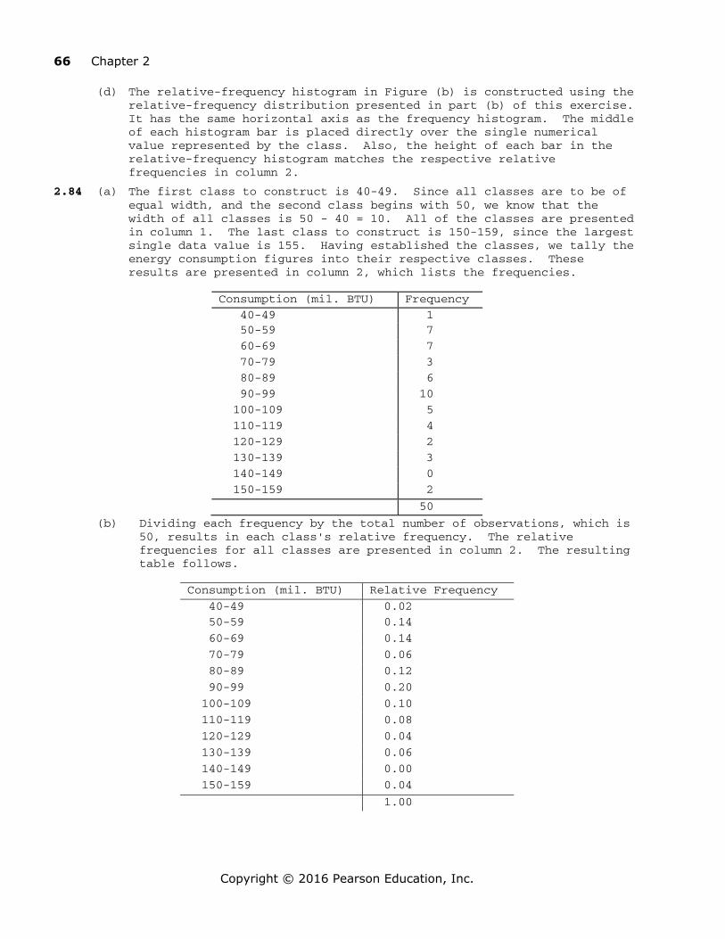
66 Chapter 2
Copyright © 2016 Pearson Education, Inc.
(d) The relative-frequency histogram in Figure (b) is constructed using the relative-frequency distribution presented in part (b) of this exercise. It has the same horizontal axis as the frequency histogram. The middle of each histogram bar is placed directly over the single numerical value represented by the class. Also, the height of each bar in the relative-frequency histogram matches the respective relative frequencies in column 2.
2.84 (a) The first class to construct is 40-49. Since all classes are to be of equal width, and the second class begins with 50, we know that the width of all classes is 50 - 40 = 10. All of the classes are presented in column 1. The last class to construct is 150-159, since the largest single data value is 155. Having established the classes, we tally the energy consumption figures into their respective classes. These results are presented in column 2, which lists the frequencies.
(b) Dividing each frequency by the total number of observations, which is 50, results in each class's relative frequency. The relative frequencies for all classes are presented in column 2. The resulting table follows.
Consumption (mil. BTU) Frequency
40-49 1 50-59 7
60-69 7
70-79 3
80-89 6
90-99 10
100-109 5
110-119 4
120-129 2
130-139 3
140-149 0
150-159 2
50
Consumption (mil. BTU) Relative Frequency
40-49 0.02
50-59 0.14
60-69 0.14
70-79 0.06
80-89 0.12
90-99 0.20
100-109 0.10
110-119 0.08
120-129 0.04
130-139 0.06
140-149 0.00
150-159 0.04
1.00

Section 2.3 67
Copyright © 2016 Pearson Education, Inc.
(c) The frequency histogram in Figure (a) is constructed using the frequency distribution presented in part (a) of this exercise. The lower class limits of column 1 are used to label the horizontal axis of the frequency histogram. Suitable candidates for vertical-axis units in the frequency histogram are the even integers 0 through 10, since these are representative of the magnitude and spread of the frequency presented in column 2. The height of each bar in the frequency histogram matches the respective frequency in column 2.
(d) The relative-frequency histogram in Figure (b) is constructed using the relative-frequency distribution presented in part (b) of this exercise. It has the same horizontal axis as the frequency histogram. We notice that the relative frequencies presented in column 2 vary in size from 0.00 to 0.20. Thus, suitable candidates for vertical axis units in the relative-frequency histogram are increments of 0.05 (or 5%), from zero to 0.20 (or 20%). The height of each bar in the relative-frequency histogram matches the respective relative frequency in column 2.
Figure (a) Figure (b)
160150140130120110100908070605040
10
8
6
4
2
0
ENERGY
Freq
uenc
y
Histogram of ENERGY
160150140130120110100908070605040
20
15
10
5
0
ENERGY
Perc
ent
Histogram of ENERGY
2.85 (a) The first class to construct is 40-44. Since all classes are to be of equal width, and the second class begins with 45, we know that the width of all classes is 45 - 40 = 5. All of the classes are presented in column 1. The last class to construct is 60-64, since the largest single data value is 61. Having established the classes, we tally the age figures into their respective classes. These results are presented in column 2, which lists the frequencies.
(b) Dividing each frequency by the total number of observations, which is 21, results in each class's relative frequency. The relative frequencies for all classes are presented in column 2. The resulting table follows.
Age Frequency 40-44 4 45-49 3 50-54 4 55-59 8 60-64 2 21

68 Chapter 2
Copyright © 2016 Pearson Education, Inc.
(c) The frequency histogram in Figure (a) is constructed using the frequency distribution presented in part (a) of this exercise. The lower class limits of column 1 are used to label the horizontal axis of the frequency histogram. Suitable candidates for vertical-axis units in the frequency histogram are the even integers 2 through 8, since these are representative of the magnitude and spread of the frequency presented in column 2. The height of each bar in the frequency histogram matches the respective frequency in column 2.
(d) The relative-frequency histogram in Figure (b) is constructed using the relative-frequency distribution presented in part (b) of this exercise. It has the same horizontal axis as the frequency histogram. We notice that the relative frequencies presented in column 2 vary in size from 0.095 to 0.381. Thus, suitable candidates for vertical axis units in the relative-frequency histogram are increments of 0.10 (or 10%), from zero to 0.40 (or 40%). The height of each bar in the relative-frequency histogram matches the respective relative frequency in column 2.
Figure (a) Figure (b)
656055504540
9
8
7
6
5
4
3
2
1
0
AGE
Freq
uenc
y
Early-Onset Dementia
656055504540
40
30
20
10
0
AGE
Perc
ent
Early-Onset Dementia
2.86 (a) The first class to construct is 20-22. Since all classes are to be of equal width, and the second class begins with 23, we know that the width of all classes is 23 - 20 = 3. All of the classes are presented in column 1. The last class to construct is 44-46, since the largest single data value is 46. Having established the classes, we tally the cheese consumption figures into their respective classes. These results are presented in column 2, which lists the frequencies.
Age Relative Frequency 40-44 0.190 45-49 0.143 50-54 0.190 55-59 0.381 60-64 0.095 1.000
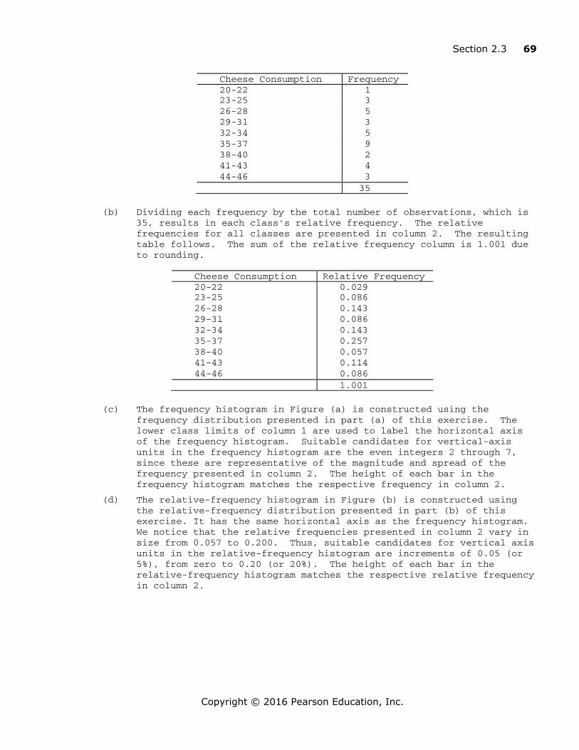
Section 2.3 69
Copyright © 2016 Pearson Education, Inc.
(b) Dividing each frequency by the total number of observations, which is 35, results in each class's relative frequency. The relative frequencies for all classes are presented in column 2. The resulting table follows. The sum of the relative frequency column is 1.001 due to rounding.
(c) The frequency histogram in Figure (a) is constructed using the frequency distribution presented in part (a) of this exercise. The lower class limits of column 1 are used to label the horizontal axis of the frequency histogram. Suitable candidates for vertical-axis units in the frequency histogram are the even integers 2 through 7, since these are representative of the magnitude and spread of the frequency presented in column 2. The height of each bar in the frequency histogram matches the respective frequency in column 2.
(d) The relative-frequency histogram in Figure (b) is constructed using the relative-frequency distribution presented in part (b) of this exercise. It has the same horizontal axis as the frequency histogram. We notice that the relative frequencies presented in column 2 vary in size from 0.057 to 0.200. Thus, suitable candidates for vertical axis units in the relative-frequency histogram are increments of 0.05 (or 5%), from zero to 0.20 (or 20%). The height of each bar in the relative-frequency histogram matches the respective relative frequency in column 2.
Cheese Consumption Frequency 20-22 1 23-25 3 26-28 5 29-31 3 32-34 5 35-37 9 38-40 2 41-43 4 44-46 3 35
Cheese Consumption Relative Frequency 20-22 0.029 23-25 0.086 26-28 0.143 29-31 0.086 32-34 0.143 35-37 0.257 38-40 0.057 41-43 0.114 44-46 0.086 1.001
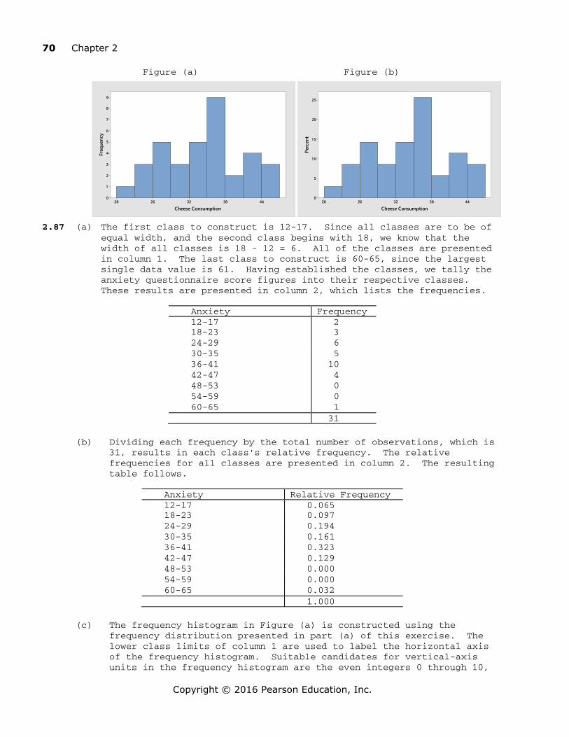
70 Chapter 2
Copyright © 2016 Pearson Education, Inc.
Figure (a) Figure (b)
4438322620
9
8
7
6
5
4
3
2
1
0
Cheese Consumption
Freq
uenc
y
4438322620
25
20
1 5
1 0
5
0
Cheese Consumption
Perc
ent
2.87 (a) The first class to construct is 12-17. Since all classes are to be of equal width, and the second class begins with 18, we know that the width of all classes is 18 - 12 = 6. All of the classes are presented in column 1. The last class to construct is 60-65, since the largest single data value is 61. Having established the classes, we tally the anxiety questionnaire score figures into their respective classes. These results are presented in column 2, which lists the frequencies.
(b) Dividing each frequency by the total number of observations, which is 31, results in each class's relative frequency. The relative frequencies for all classes are presented in column 2. The resulting table follows.
(c) The frequency histogram in Figure (a) is constructed using the frequency distribution presented in part (a) of this exercise. The lower class limits of column 1 are used to label the horizontal axis of the frequency histogram. Suitable candidates for vertical-axis units in the frequency histogram are the even integers 0 through 10,
Anxiety Frequency 12-17 2 18-23 3 24-29 6 30-35 5 36-41 10 42-47 4 48-53 0 54-59 0 60-65 1 31
Anxiety Relative Frequency 12-17 0.065 18-23 0.097 24-29 0.194 30-35 0.161 36-41 0.323 42-47 0.129 48-53 0.000 54-59 0.000 60-65 0.032 1.000
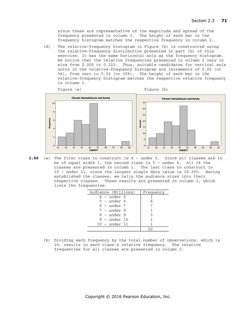
Section 2.3 71
Copyright © 2016 Pearson Education, Inc.
since these are representative of the magnitude and spread of the frequency presented in column 2. The height of each bar in the frequency histogram matches the respective frequency in column 2.
(d) The relative-frequency histogram in Figure (b) is constructed using the relative-frequency distribution presented in part (b) of this exercise. It has the same horizontal axis as the frequency histogram. We notice that the relative frequencies presented in column 2 vary in size from 0.000 to 0.323. Thus, suitable candidates for vertical axis units in the relative-frequency histogram are increments of 0.05 (or 5%), from zero to 0.35 (or 35%). The height of each bar in the relative-frequency histogram matches the respective relative frequency in column 2.
Figure (a) Figure (b)
66605448423630241812
10
8
6
4
2
0
ANXIETY
Freq
uenc
y
Chronic Hemodialysis and Axiety
66605448423630241812
35
30
25
20
15
10
5
0
ANXIETY
Perc
ent
Chronic Hemodialysis and Axiety
2.88 (a) The first class to construct is 4 – under 5. Since all classes are to be of equal width 1, the second class is 5 – under 6. All of the classes are presented in column 1. The last class to construct is 10 – under 11, since the largest single data value is 10.360. Having established the classes, we tally the audience sizes into their respective classes. These results are presented in column 2, which lists the frequencies.
Audience (Millions) Frequency 4 – under 5 1 5 – under 6 6 6 – under 7 7 7 – under 8 1 8 – under 9 3 9 – under 10 1 10 – under 11 1 20
(b) Dividing each frequency by the total number of observations, which is 20, results in each class's relative frequency. The relative frequencies for all classes are presented in column 2.
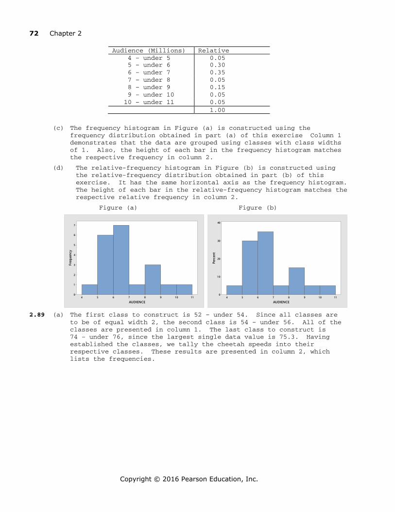
72 Chapter 2
Copyright © 2016 Pearson Education, Inc.
Audience (Millions) Relative 4 – under 5 0.05 5 – under 6 0.30 6 – under 7 0.35 7 – under 8 0.05 8 – under 9 0.15 9 – under 10 0.05 10 – under 11 0.05 1.00
(c) The frequency histogram in Figure (a) is constructed using the frequency distribution obtained in part (a) of this exercise Column 1 demonstrates that the data are grouped using classes with class widths of 1. Also, the height of each bar in the frequency histogram matches the respective frequency in column 2.
(d) The relative-frequency histogram in Figure (b) is constructed using the relative-frequency distribution obtained in part (b) of this exercise. It has the same horizontal axis as the frequency histogram. The height of each bar in the relative-frequency histogram matches the respective relative frequency in column 2.
Figure (a) Figure (b)
1 11 0987654
7
6
5
4
3
2
1
0
AUDIENCE
Freq
uenc
y
1 11 0987654
40
30
20
1 0
0
AUDIENCE
Perc
ent
2.89 (a) The first class to construct is 52 – under 54. Since all classes are to be of equal width 2, the second class is 54 – under 56. All of the classes are presented in column 1. The last class to construct is 74 – under 76, since the largest single data value is 75.3. Having established the classes, we tally the cheetah speeds into their respective classes. These results are presented in column 2, which lists the frequencies.
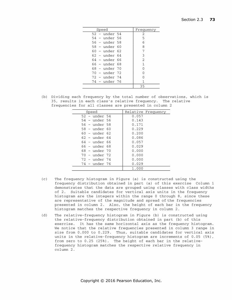
Section 2.3 73
Copyright © 2016 Pearson Education, Inc.
Speed Frequency 52 – under 54 2 54 – under 56 5 56 – under 58 6 58 – under 60 8 60 – under 62 7 62 – under 64 3 64 – under 66 2 66 – under 68 1 68 – under 70 0 70 – under 72 0 72 – under 74 0 74 – under 76 1 35
(b) Dividing each frequency by the total number of observations, which is 35, results in each class's relative frequency. The relative frequencies for all classes are presented in column 2
Speed Relative Frequency 52 – under 54 0.057 54 – under 56 0.143 56 – under 58 0.171 58 – under 60 0.229 60 – under 62 0.200 62 – under 64 0.086 64 – under 66 0.057 66 – under 68 0.029 68 – under 70 0.000 70 – under 72 0.000 72 – under 74 0.000 74 – under 76 0.029 1.000
(c) The frequency histogram in Figure (a) is constructed using the frequency distribution obtained in part (a) of this exercise Column 1 demonstrates that the data are grouped using classes with class widths of 2. Suitable candidates for vertical axis units in the frequency histogram are the integers within the range 0 through 8, since these are representative of the magnitude and spread of the frequencies presented in column 2. Also, the height of each bar in the frequency histogram matches the respective frequency in column 2.
(d) The relative-frequency histogram in Figure (b) is constructed using the relative-frequency distribution obtained in part (b) of this exercise. It has the same horizontal axis as the frequency histogram. We notice that the relative frequencies presented in column 3 range in size from 0.000 to 0.229. Thus, suitable candidates for vertical axis units in the relative-frequency histogram are increments of 0.05 (5%), from zero to 0.25 (25%). The height of each bar in the relative-frequency histogram matches the respective relative frequency in column 2.
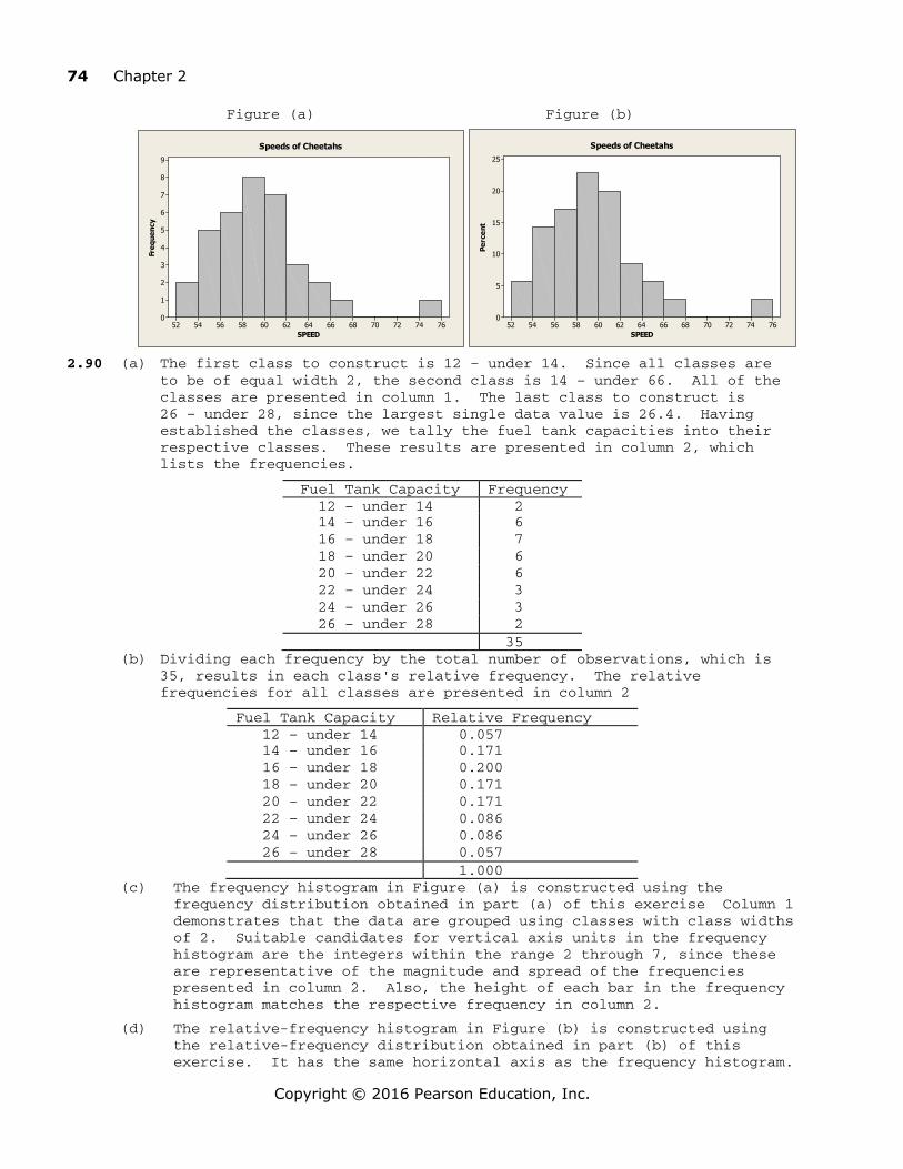
74 Chapter 2
Copyright © 2016 Pearson Education, Inc.
Figure (a) Figure (b)
76747270686664626058565452
9
8
7
6
5
4
3
2
1
0
SPEED
Freq
uenc
ySpeeds of Cheetahs
76747270686664626058565452
25
20
15
10
5
0
SPEED
Perc
ent
Speeds of Cheetahs
2.90 (a) The first class to construct is 12 – under 14. Since all classes are to be of equal width 2, the second class is 14 – under 66. All of the classes are presented in column 1. The last class to construct is 26 – under 28, since the largest single data value is 26.4. Having established the classes, we tally the fuel tank capacities into their respective classes. These results are presented in column 2, which lists the frequencies.
Fuel Tank Capacity Frequency 12 – under 14 2 14 – under 16 6 16 – under 18 7 18 – under 20 6 20 – under 22 6 22 – under 24 3 24 – under 26 3 26 – under 28 2 35
(b) Dividing each frequency by the total number of observations, which is 35, results in each class's relative frequency. The relative frequencies for all classes are presented in column 2
Fuel Tank Capacity Relative Frequency 12 – under 14 0.057 14 – under 16 0.171 16 – under 18 0.200 18 – under 20 0.171 20 – under 22 0.171 22 – under 24 0.086 24 – under 26 0.086 26 – under 28 0.057 1.000
(c) The frequency histogram in Figure (a) is constructed using the frequency distribution obtained in part (a) of this exercise Column 1 demonstrates that the data are grouped using classes with class widths of 2. Suitable candidates for vertical axis units in the frequency histogram are the integers within the range 2 through 7, since these are representative of the magnitude and spread of the frequencies presented in column 2. Also, the height of each bar in the frequency histogram matches the respective frequency in column 2.
(d) The relative-frequency histogram in Figure (b) is constructed using the relative-frequency distribution obtained in part (b) of this exercise. It has the same horizontal axis as the frequency histogram.
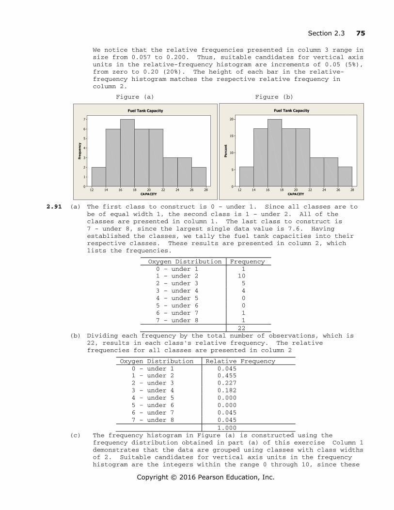
Section 2.3 75
Copyright © 2016 Pearson Education, Inc.
We notice that the relative frequencies presented in column 3 range in size from 0.057 to 0.200. Thus, suitable candidates for vertical axis units in the relative-frequency histogram are increments of 0.05 (5%), from zero to 0.20 (20%). The height of each bar in the relative-frequency histogram matches the respective relative frequency in column 2.
Figure (a) Figure (b)
282624222018161412
7
6
5
4
3
2
1
0
CAPACITY
Freq
uenc
y
Fuel Tank Capacity
282624222018161412
20
15
10
5
0
CAPACITY
Perc
ent
Fuel Tank Capacity
2.91 (a) The first class to construct is 0 – under 1. Since all classes are to be of equal width 1, the second class is 1 – under 2. All of the classes are presented in column 1. The last class to construct is 7 - under 8, since the largest single data value is 7.6. Having established the classes, we tally the fuel tank capacities into their respective classes. These results are presented in column 2, which lists the frequencies.
Oxygen Distribution Frequency 0 – under 1 1 1 – under 2 10 2 – under 3 5 3 – under 4 4 4 – under 5 0 5 – under 6 0 6 – under 7 1 7 – under 8 1 22
(b) Dividing each frequency by the total number of observations, which is 22, results in each class's relative frequency. The relative frequencies for all classes are presented in column 2
Oxygen Distribution Relative Frequency 0 – under 1 0.045 1 – under 2 0.455 2 – under 3 0.227 3 – under 4 0.182 4 – under 5 0.000 5 – under 6 0.000 6 – under 7 0.045 7 – under 8 0.045 1.000
(c) The frequency histogram in Figure (a) is constructed using the frequency distribution obtained in part (a) of this exercise Column 1 demonstrates that the data are grouped using classes with class widths of 2. Suitable candidates for vertical axis units in the frequency histogram are the integers within the range 0 through 10, since these

76 Chapter 2
Copyright © 2016 Pearson Education, Inc.
are representative of the magnitude and spread of the frequencies presented in column 2. Also, the height of each bar in the frequency histogram matches the respective frequency in column 2.
(d) The relative-frequency histogram in Figure (b) is constructed using the relative-frequency distribution obtained in part (b) of this exercise. It has the same horizontal axis as the frequency histogram. We notice that the relative frequencies presented in column 3 range in size from 0.000 to 0.455. Thus, suitable candidates for vertical axis units in the relative-frequency histogram are increments of 0.05 (5%), from zero to 0.50 (50%). The height of each bar in the relative-frequency histogram matches the respective relative frequency in column 2.
Figure (a) Figure (b)
876543210
10
8
6
4
2
0
OXYGEN
Freq
uenc
y
Oxygen Distribution
876543210
50
40
30
20
10
0
OXYGEN
Perc
ent
Oxygen Distribution
2.92 The horizontal axis of this dotplot displays a range of possible exam scores. To complete the dotplot, we go through the data set and record each exam score by placing a dot over the appropriate value on the horizontal axis.
2.93 The horizontal axis of this dotplot displays of range of possible ages of the passenger cars. To complete the dotplot, we go through the data set and record each age by placing a dot over the appropriate value on the horizontal axis.
SCORE9990817263544536
Dotplot of SCORE
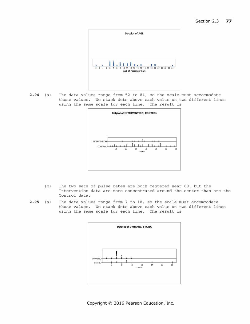
Section 2.3 77
Copyright © 2016 Pearson Education, Inc.
24232221201 91 81 71 61 51 41 31 21 11 098765432AGE of Passenger Cars
Dotplot of AGE
2.94 (a) The data values range from 52 to 84, so the scale must accommodate those values. We stack dots above each value on two different lines using the same scale for each line. The result is
(b) The two sets of pulse rates are both centered near 68, but the Intervention data are more concentrated around the center than are the Control data.
2.95 (a) The data values range from 7 to 18, so the scale must accommodate those values. We stack dots above each value on two different lines using the same scale for each line. The result is
Data85807570656055
INTERVENTION
CONTROL
Dotplot of INTERVENTION, CONTROL
Data181614121086
DYNAMIC
STATIC
Dotplot of DYNAMIC, STATIC

78 Chapter 2
Copyright © 2016 Pearson Education, Inc.
(b) The Dynamic system does seem to reduce acute postoperative days in the hospital on the average. The Dynamic data are centered at about 7 days, whereas the Static data are centered at about 11 days and are much more spread out than the Dynamic data.
2.96 The data values consist of 2 digit numbers followed by a one digit decimal place ranging from 45.5 to 57.0. The last digit following the decimal will be the leaves and the stems will be the remaining digits. Therefore, the stem-and-leaf diagram will have stems of 45 through 57.
45| 5 46| 4 47| 2 48| 0 49| 1 50| 3578 51| 35589 52| 011 53| 355689 54| 13 55| 033 56| 0 57| 0
2.97 Since each data value consists of 2 digits, each beginning with 1, 2, 3, or 4, we will construct the stem-and-leaf diagram with these four values as the stems. The result is
1| 238 2| 1678899 3| 34459 4| 04
2.98 (a) Since each data value consists of a 2 digit number with a one digit decimal, we will make the leaf the decimal digit and the stems the remaining two digit numbers of 28, 29, 30, and 31. The result is
28| 8 29| 368 30| 1247 31| 02
(b) Splitting into two lines per stem, leafs of 0-4 belong in the first stem and leafs of 5-9 belong in the second stem. The result is
28| 8 29| 3 29| 68 30| 124 30| 7 31| 02
(c) The stem-and-leaf diagram in part (b) is more useful because by splitting the stems into two lines per stem, you have created more lines. Part (a) had too few lines.
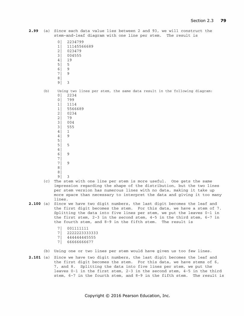
Section 2.3 79
Copyright © 2016 Pearson Education, Inc.
2.99 (a) Since each data value lies between 2 and 93, we will construct the stem-and-leaf diagram with one line per stem. The result is
0| 2234799 1| 11145566689 2| 023479 3| 004555 4| 19 5| 5 6| 9 7| 9 8| 9| 3
(b) Using two lines per stem, the same data result in the following diagram: 0| 2234
0| 799 1| 1114 1| 5566689 2| 0234 2| 79 3| 004 3| 555 4| 1 4| 9 5| 5| 5 6| 6| 9 7| 7| 9 8| 8| 9| 3
(c) The stem with one line per stem is more useful. One gets the same impression regarding the shape of the distribution, but the two lines per stem version has numerous lines with no data, making it take up more space than necessary to interpret the data and giving it too many lines.
2.100 (a) Since we have two digit numbers, the last digit becomes the leaf and the first digit becomes the stem. For this data, we have a stem of 7. Splitting the data into five lines per stem, we put the leaves 0-1 in the first stem, 2-3 in the second stem, 4-5 in the third stem, 6-7 in the fourth stem, and 8-9 in the fifth stem. The result is
7| 001111111 7| 2222223333333 7| 444444445555 7| 66666666677
(b) Using one or two lines per stem would have given us too few lines.
2.101 (a) Since we have two digit numbers, the last digit becomes the leaf and the first digit becomes the stem. For this data, we have stems of 6, 7, and 8. Splitting the data into five lines per stem, we put the leaves 0-1 in the first stem, 2-3 in the second stem, 4-5 in the third stem, 6-7 in the fourth stem, and 8-9 in the fifth stem. The result is
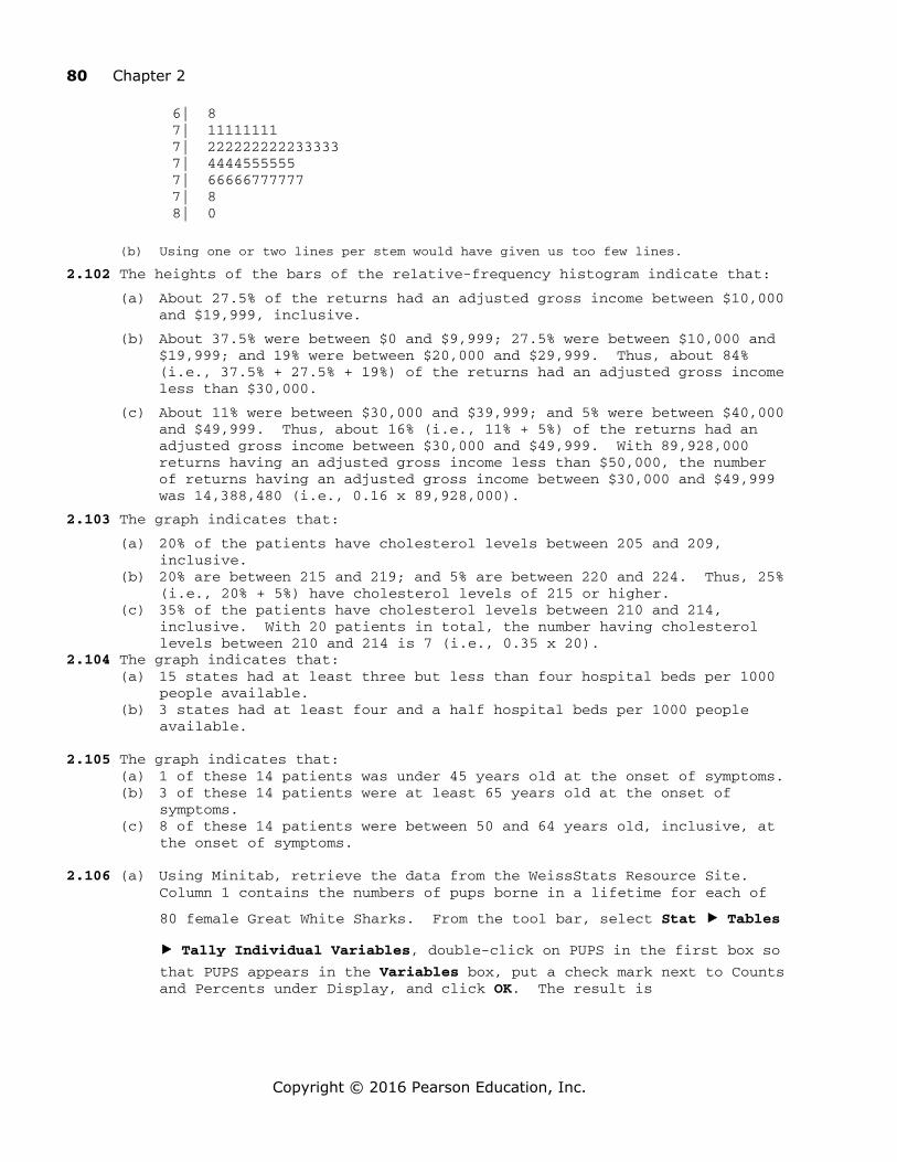
80 Chapter 2
Copyright © 2016 Pearson Education, Inc.
6| 8 7| 11111111 7| 222222222233333 7| 4444555555 7| 66666777777 7| 8 8| 0
(b) Using one or two lines per stem would have given us too few lines.
2.102 The heights of the bars of the relative-frequency histogram indicate that:
(a) About 27.5% of the returns had an adjusted gross income between $10,000 and $19,999, inclusive.
(b) About 37.5% were between $0 and $9,999; 27.5% were between $10,000 and $19,999; and 19% were between $20,000 and $29,999. Thus, about 84% (i.e., 37.5% + 27.5% + 19%) of the returns had an adjusted gross income less than $30,000.
(c) About 11% were between $30,000 and $39,999; and 5% were between $40,000 and $49,999. Thus, about 16% (i.e., 11% + 5%) of the returns had an adjusted gross income between $30,000 and $49,999. With 89,928,000 returns having an adjusted gross income less than $50,000, the number of returns having an adjusted gross income between $30,000 and $49,999 was 14,388,480 (i.e., 0.16 x 89,928,000).
2.103 The graph indicates that:
(a) 20% of the patients have cholesterol levels between 205 and 209, inclusive.
(b) 20% are between 215 and 219; and 5% are between 220 and 224. Thus, 25% (i.e., 20% + 5%) have cholesterol levels of 215 or higher.
(c) 35% of the patients have cholesterol levels between 210 and 214, inclusive. With 20 patients in total, the number having cholesterol levels between 210 and 214 is 7 (i.e., 0.35 x 20).
2.104 The graph indicates that: (a) 15 states had at least three but less than four hospital beds per 1000
people available. (b) 3 states had at least four and a half hospital beds per 1000 people
available. 2.105 The graph indicates that: (a) 1 of these 14 patients was under 45 years old at the onset of symptoms. (b) 3 of these 14 patients were at least 65 years old at the onset of
symptoms. (c) 8 of these 14 patients were between 50 and 64 years old, inclusive, at
the onset of symptoms. 2.106 (a) Using Minitab, retrieve the data from the WeissStats Resource Site.
Column 1 contains the numbers of pups borne in a lifetime for each of
80 female Great White Sharks. From the tool bar, select Stat < Tables < Tally Individual Variables, double-click on PUPS in the first box so that PUPS appears in the Variables box, put a check mark next to Counts and Percents under Display, and click OK. The result is

Section 2.3 81
Copyright © 2016 Pearson Education, Inc.
PUPS Count Percent
3 2 2.50
4 5 6.25
5 10 12.50
6 11 13.75
7 17 21.25
8 17 21.25
9 11 13.75
10 4 5.00
11 2 2.50
12 1 1.25
(b) After retrieving the data from the WeissStats Resource Site, select
Graph < Histogram, choose Simple and click OK. Double click on PUPS in the first box to enter PUPS in the Graphs variables box, and click OK. The frequency histogram is
To change to a relative-frequency histogram, before clicking OK the second time, click on the Scale button and the Y-Scale type tab, and choose Percent and click OK. The graph will look like the frequency histogram, but will have relative frequencies on the vertical scale instead of counts.
The numbers of pups range from 1 to 12 per female with 7 and 8 pups occurring more frequently than any other values.
2.107 (a) Using Minitab, there is not a direct way to get a grouped frequency distribution. However, you can use an option in creating your histogram that will report the frequencies in each of the classes, essentially creating a grouped frequency distribution. Retrieve the data from the WeissStats Resource Site. Column 2 contains the length
of the Beatles songs, in seconds. From the tool bar, select Graph < Histogram, choose Simple and click OK. Double click on LENGTH to enter LENGTH in the Graph variables box. Click Labels, click the Data Labels tab, then check Use y-value labels. Click OK twice. The result is
PUPS
Freq
uenc
y
1210864
18
16
14
12
10
8
6
4
2
0
Histogram of PUPS

82 Chapter 2
Copyright © 2016 Pearson Education, Inc.
4503753002251 5075
70
60
50
40
30
20
1 0
0
LENGTHFr
eque
ncy
1101100113
8
1317
42
70
54
9
331
Above each bar is a label for each of the frequencies. Also, the labeling on the horizontal axis is the midpoint for class, where each class has a width of 25. To change the width of the bars, right Click on the bars and choose Edit Bars, click Binning, click Midpoint/Cutpoint positions:, type 0 50 100 150 200 250 300 350 400 450 500. The result is
5004003002001 000
1 40
1 20
1 00
80
60
40
20
0
LENGTH
Freq
uenc
y
12112
18
42
124
32
51
To get the relative-frequency distribution, follow the same steps as above, but also Click the Scale button, click the Y-scale Type, check Percent, then click OK twice. The result is
5004003002001000
60
50
40
30
20
10
0
LENGTH
Perc
ent
0.4366810.8733620.4366810.4366810.873362
7.86026
18.3406
54.1485
13.9738
2.183410.436681
Above each bar is the percentage for that class, essentially creating a
relative-frequency distribution. You could also transfer these results into a table.
(b) A frequency histogram and a relative frequency distribution were created in part (a).

Section 2.3 83
Copyright © 2016 Pearson Education, Inc.
(c) To obtain the dotplot, select Graph < Dotplot, select Simple in the One Y row, and click OK. Double click on LENGTH to enter LEGNTH in the Graph variables box and click OK. The result is
49042035028021 01 4070LENGTH
Dotplot of LENGTH
(d) The graphs are similar, but not identical. This is because the dotplot preserves the raw data by plotting individual dots and the histogram looses the raw data because it groups observations into grouped classes. The overall impression, however, remains the same. They both are generally the same shape with outliers to the right.
2.108 (a) After entering the data from the WeissStats Resource Site, in Minitab,
select Graph < Stem-and-Leaf, double click on PERCENT to enter PERCENT in the Graph variables box and enter a 10 in the Increment box, and click OK. The result is
Stem-and-leaf of PERCENT N = 51 Leaf Unit = 1.0
(35) 8 00122223334444455566777777888889999 16 9 0000000001111122
(b) Repeat part (a), but this time enter a 5 in the Increment box. The
result is
Stem-and-leaf of PERCENT N = 51 Leaf Unit = 1.0
15 8 001222233344444 (20) 8 55566777777888889999
16 9 0000000001111122
(c) Repeat part (a) again, but this time enter a 2 in the Increment box. The result is
Stem-and-leaf of PERCENT N = 51 Leaf Unit = 1.0
3 8 001
10 8 2222333 18 8 44444555 (8) 8 66777777
25 8 888889999 16 9 00000000011111 2 9 22
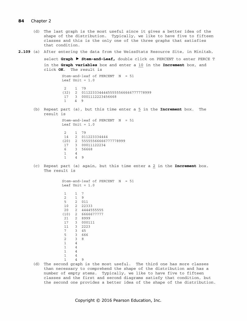
84 Chapter 2
Copyright © 2016 Pearson Education, Inc.
(d) The last graph is the most useful since it gives a better idea of the shape of the distribution. Typically, we like to have five to fifteen classes and this is the only one of the three graphs that satisfies that condition.
2.109 (a) After entering the data from the WeissStats Resource Site, in Minitab,
select Graph < Stem-and-Leaf, double click on PERCENT to enter PERCE T in the Graph variables box and enter a 10 in the Increment box, and click OK. The result is
Stem-and-leaf of PERCENT N = 51 Leaf Unit = 1.0
2 1 79 (32) 2 01122333444455555566666777778999 17 3 0001112223456668 1 4 9
(b) Repeat part (a), but this time enter a 5 in the Increment box. The
result is
Stem-and-leaf of PERCENT N = 51 Leaf Unit = 1.0
2 1 79 14 2 011223334444 (20) 2 55555566666777778999 17 3 00011122234 6 3 56668 1 4 1 4 9
(c) Repeat part (a) again, but this time enter a 2 in the Increment box.
The result is
Stem-and-leaf of PERCENT N = 51 Leaf Unit = 1.0
1 1 7 2 1 9 5 2 011 10 2 22333 20 2 4444555555 (10) 2 6666677777 21 2 8999 17 3 000111 11 3 2223 7 3 45 5 3 666 2 3 8 1 4 1 4 1 4 1 4 1 4 9
(d) The second graph is the most useful. The third one has more classes than necessary to comprehend the shape of the distribution and has a number of empty stems. Typically, we like to have five to fifteen classes and the first and second diagrams satisfy that condition, but the second one provides a better idea of the shape of the distribution.
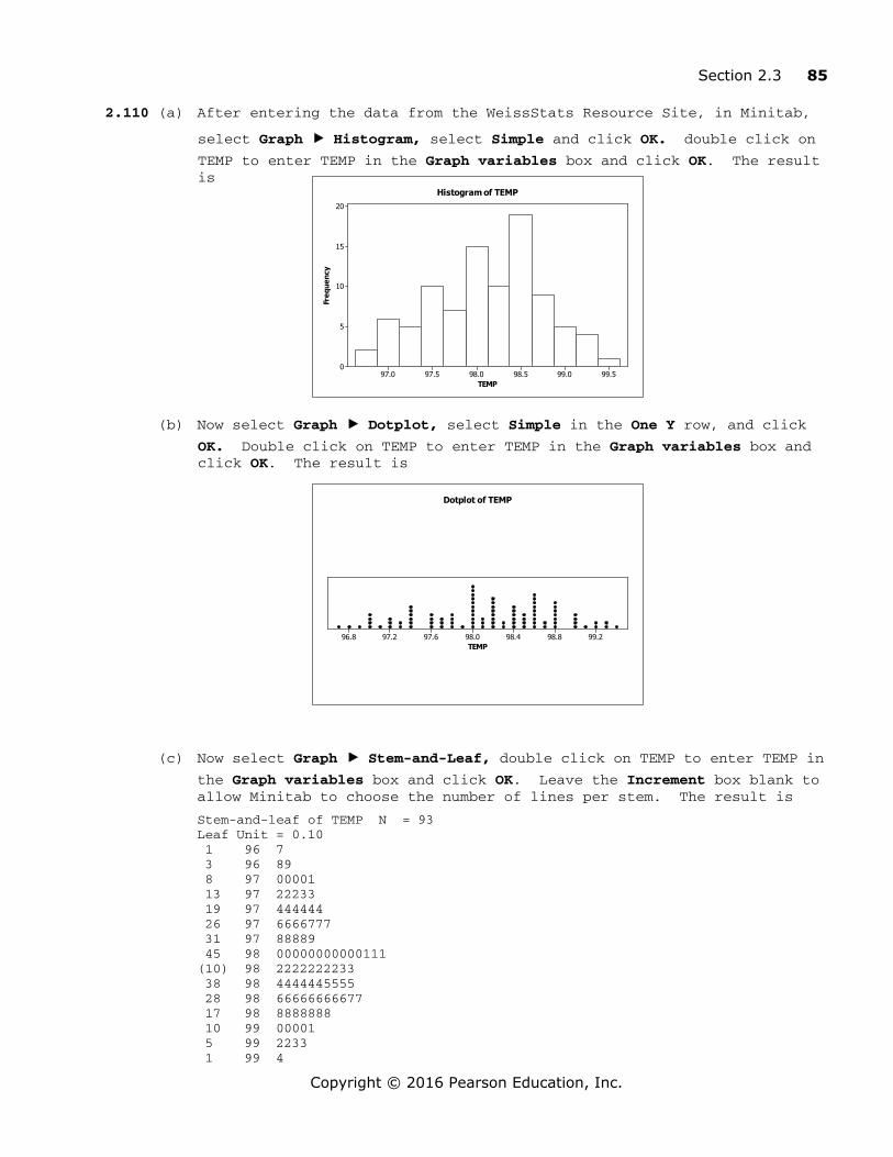
Section 2.3 85
Copyright © 2016 Pearson Education, Inc.
TEMP
Freq
uenc
y
99.599.098.598.097.597.0
20
15
10
5
0
Histogram of TEMP
TEMP99.298.898.498.097.697.296.8
Dotplot of TEMP
2.110 (a) After entering the data from the WeissStats Resource Site, in Minitab,
select Graph < Histogram, select Simple and click OK. double click on TEMP to enter TEMP in the Graph variables box and click OK. The result is
(b) Now select Graph < Dotplot, select Simple in the One Y row, and click OK. Double click on TEMP to enter TEMP in the Graph variables box and click OK. The result is
(c) Now select Graph < Stem-and-Leaf, double click on TEMP to enter TEMP in the Graph variables box and click OK. Leave the Increment box blank to allow Minitab to choose the number of lines per stem. The result is
Stem-and-leaf of TEMP N = 93 Leaf Unit = 0.10 1 96 7 3 96 89 8 97 00001 13 97 22233 19 97 444444 26 97 6666777 31 97 88889 45 98 00000000000111 (10) 98 2222222233 38 98 4444445555 28 98 66666666677 17 98 8888888 10 99 00001 5 99 2233 1 99 4

86 Chapter 2
Copyright © 2016 Pearson Education, Inc.
(d) The dotplot shows all of the individual values. The stem-and-leaf diagram used five lines per stem and therefore each line contains leaves with possibly two values. The histogram chose classes of width 0.25. This resulted in, for example, the class with midpoint 97.0 including all of the values 96.9, 97.0, and 97.1, while the class with midpoint 97.25 includes only the two values 97.2 and 97.3. Thus the ‘smoothing’ effect is not as good in the histogram as it is in the stem-and-leaf diagram. Overall, the dotplot gives the truest picture of the data and allows recovery of all of the data values.
2.111 (a) The classes are presented in column 1. With the classes established, we then tally the exam scores into their respective classes. These results are presented in column 2, which lists the frequencies. Dividing each frequency by the total number of exam scores, which is 20, results in each class's relative frequency. The relative frequencies for all classes are presented in column 3. The class mark of each class is the average of the lower and upper limits. The class marks for all classes are presented in column 4.
Score Frequency Relative Frequency Class Mark
30-39 2 0.10 34.5
40-49 0 0.00 44.5 50-59 0 0.00 54.5 60-69 3 0.15 64.5 70-79 3 0.15 74.5 80-89 8 0.40 84.5 90-100 4 0.20 95.0 20 1.00
(b) The first six classes have width 10; the seventh class had width 11.
(c) Answers will vary, but one choice is to keep the first six classes the same and make the next two classes 90-99 and 100-109. Another possibility is 31-40, 41-50, …, 91-100.
2.112 Answers will vary, but by following the steps we first decide on the approximate number of classes. Since there are 40 observations, we should have 7-14 classes. This exercise states we should have approximately seven classes. Step 2 says that we calculate an approximate class width as (99 – 36)/7 = 9. A convenient class width close to 9 would be a class width of 10. Step 3 says that we choose a number for the lower class limit which is less than or equal to our minimum observation of 36. Let’s choose 35. Beginning with a lower class limit of 35 and width of 10, we have a first class of 35-44, a second class of 45-54, a third class of 55-64, a fourth class of 65-74, a fifth class of 75-84, a sixth class of 85-94, and a seventh class of 95-104. This would be our last class since the largest observation is 99.
2.113 Answers will vary, but by following the steps we first decide on the approximate number of classes. Since there are 37 observations, we should have 7-14 classes. This exercise states we should have approximately eight classes. Step 2 says that we calculate an approximate class width as (278.8 – 129.2)/8 = 18.7. A convenient class width close to 18.7 would be a class width of 20. Step 3 says that we choose a number for the lower cutpoint which is less than or equal to our minimum observation of 129.2. Let’s choose 120. Beginning with a lower cutpoint of 120 and width of 20, we have a first class of 120 – under 140, a second class of 140 – under 160, a third class of 160 – under 180, a fourth class of 180 - under 200, a fifth
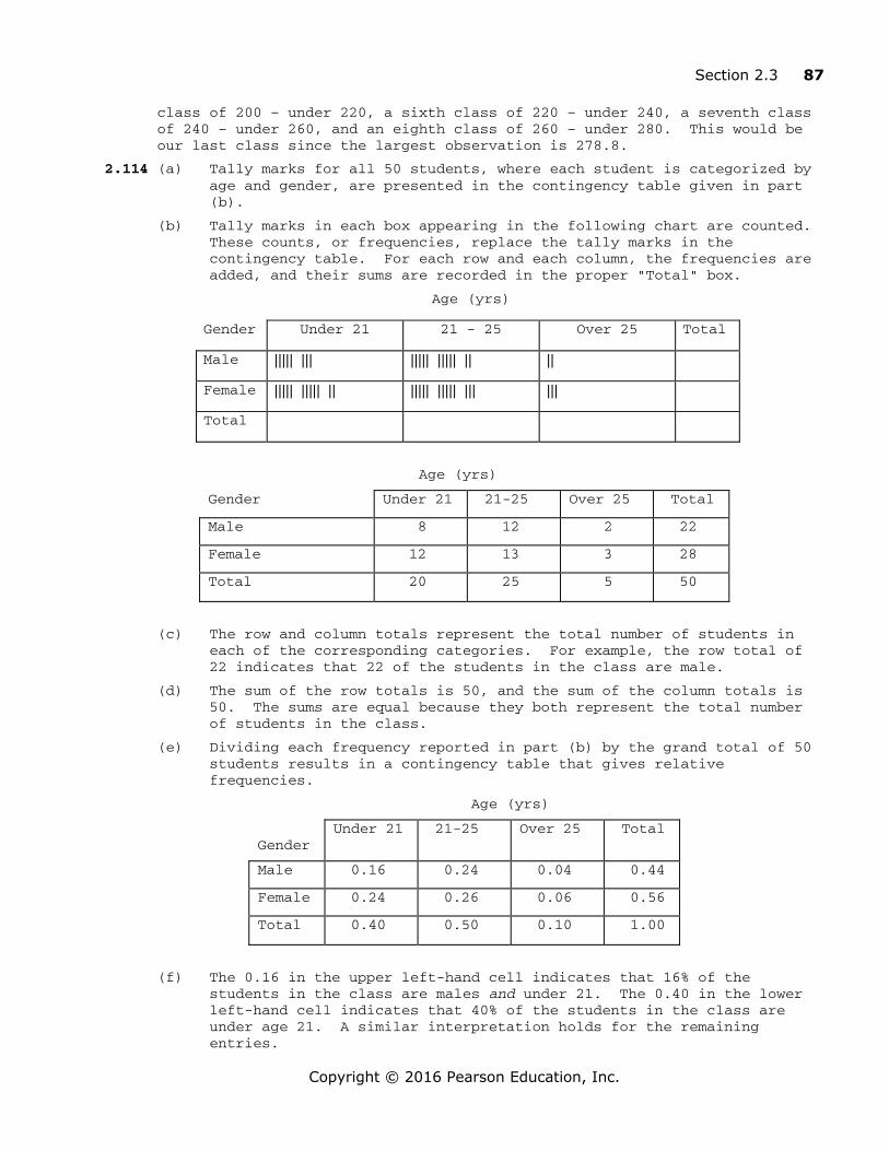
Section 2.3 87
Copyright © 2016 Pearson Education, Inc.
class of 200 – under 220, a sixth class of 220 – under 240, a seventh class of 240 – under 260, and an eighth class of 260 – under 280. This would be our last class since the largest observation is 278.8.
2.114 (a) Tally marks for all 50 students, where each student is categorized by age and gender, are presented in the contingency table given in part (b).
(b) Tally marks in each box appearing in the following chart are counted. These counts, or frequencies, replace the tally marks in the contingency table. For each row and each column, the frequencies are added, and their sums are recorded in the proper "Total" box.
Age (yrs)
Gender Under 21 21 - 25 Over 25 Total
Male ||||| ||| ||||| ||||| || ||
Female ||||| ||||| || ||||| ||||| ||| |||
Total
Age (yrs)
Gender Under 21 21-25 Over 25 Total
Male 8 12 2 22
Female 12 13 3 28
Total 20 25 5 50
(c) The row and column totals represent the total number of students in each of the corresponding categories. For example, the row total of 22 indicates that 22 of the students in the class are male.
(d) The sum of the row totals is 50, and the sum of the column totals is 50. The sums are equal because they both represent the total number of students in the class.
(e) Dividing each frequency reported in part (b) by the grand total of 50 students results in a contingency table that gives relative frequencies.
Age (yrs)
Gender
Under 21 21-25 Over 25 Total
Male 0.16 0.24 0.04 0.44
Female 0.24 0.26 0.06 0.56
Total 0.40 0.50 0.10 1.00
(f) The 0.16 in the upper left-hand cell indicates that 16% of the students in the class are males and under 21. The 0.40 in the lower left-hand cell indicates that 40% of the students in the class are under age 21. A similar interpretation holds for the remaining entries.

88 Chapter 2
Copyright © 2016 Pearson Education, Inc.
2.115 Consider columns 1 and 2 of the energy-consumption data given in Exercise 2.56 part (b). Compute the class mark for each class presented in column 1. Pair each class mark with its corresponding relative frequency found in column 2. Construct a horizontal axis, where the units are in terms of class marks and a vertical axis where the units are in terms of relative frequencies. For each class mark on the horizontal axis, plot a point whose height is equal to the relative frequency of the class. Then join the points with connecting lines. The result is a relative-frequency polygon.
2.116 Consider columns 1 and 2 of the Cheetah speed data given in Exercise 2.61 part (b). Compute the midpoint for each class presented in column 1. Pair each midpoint with its corresponding relative frequency found in column 2. Construct a horizontal axis, where the units are in terms of midpoints and a vertical axis where the units are in terms of relative frequencies. For each midpoint on the horizontal axis, plot a point whose height is equal to the relative frequency of the class. Then join the points with connecting lines. The result is a relative-frequency polygon.
757371696765636159575553
0.25
0.20
0.15
0.10
0.05
0.00
Speed (mph)
Rela
tive
Freq
uenc
y
Cheetah Speeds
2.117 In single value grouping the horizontal axis would be labeled with the value of each class.
2.118 (a) Consider parts (a) and (b) of the energy-consumption data given in Exercise 2.56. The classes are now reworked to present just the lower class limit of each class. The frequencies are reworked to sum the frequencies of all classes representing values less than the specified lower class limit. These successive sums are the cumulative frequencies. The relative frequencies are reworked to sum the relative frequencies of all classes representing values less than the specified class limits. These successive sums are the cumulative relative frequencies. (Note: The cumulative relative frequencies can
Residential Energy Consumption
0.00
0.05
0.10
0.15
0.20
0.25
35 45 55 65 75 85 95 105 115 125 135 145 155 165
BTU (Millions)
Rel
ativ
e Fr
eque
ncy
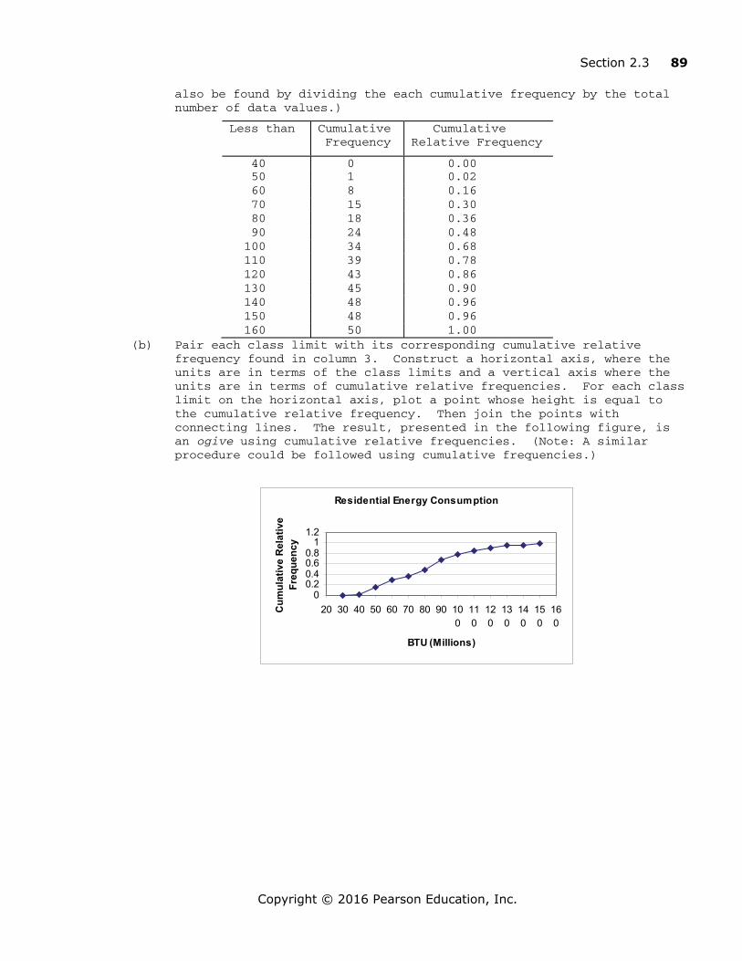
Section 2.3 89
Copyright © 2016 Pearson Education, Inc.
Residential Energy Consumption
00.20.40.60.8
11.2
20 30 40 50 60 70 80 90 100
110
120
130
140
150
160
BTU (Millions)
Cum
ulat
ive
Rel
ativ
e Fr
eque
ncy
also be found by dividing the each cumulative frequency by the total number of data values.)
Less than Cumulative Frequency
Cumulative Relative Frequency
40 0 0.00 50 1 0.02 60 8 0.16 70 15 0.30 80 18 0.36 90 24 0.48 100 34 0.68 110 39 0.78 120 43 0.86 130 45 0.90 140 48 0.96 150 48 0.96 160 50 1.00
(b) Pair each class limit with its corresponding cumulative relative frequency found in column 3. Construct a horizontal axis, where the units are in terms of the class limits and a vertical axis where the units are in terms of cumulative relative frequencies. For each class limit on the horizontal axis, plot a point whose height is equal to the cumulative relative frequency. Then join the points with connecting lines. The result, presented in the following figure, is an ogive using cumulative relative frequencies. (Note: A similar procedure could be followed using cumulative frequencies.)
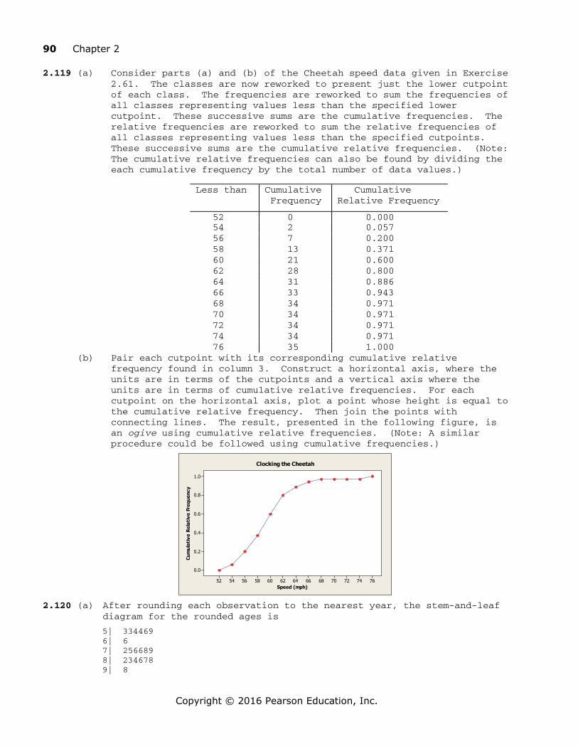
90 Chapter 2
Copyright © 2016 Pearson Education, Inc.
2.119 (a) Consider parts (a) and (b) of the Cheetah speed data given in Exercise 2.61. The classes are now reworked to present just the lower cutpoint of each class. The frequencies are reworked to sum the frequencies of all classes representing values less than the specified lower cutpoint. These successive sums are the cumulative frequencies. The relative frequencies are reworked to sum the relative frequencies of all classes representing values less than the specified cutpoints. These successive sums are the cumulative relative frequencies. (Note: The cumulative relative frequencies can also be found by dividing the each cumulative frequency by the total number of data values.)
(b) Pair each cutpoint with its corresponding cumulative relative frequency found in column 3. Construct a horizontal axis, where the units are in terms of the cutpoints and a vertical axis where the units are in terms of cumulative relative frequencies. For each cutpoint on the horizontal axis, plot a point whose height is equal to the cumulative relative frequency. Then join the points with connecting lines. The result, presented in the following figure, is an ogive using cumulative relative frequencies. (Note: A similar procedure could be followed using cumulative frequencies.)
76747270686664626058565452
1.0
0.8
0.6
0.4
0.2
0.0
Speed (mph)
Cum
ulat
ive
Rela
tive
Freq
uenc
y
Clocking the Cheetah
2.120 (a) After rounding each observation to the nearest year, the stem-and-leaf
diagram for the rounded ages is
5| 334469 6| 6 7| 256689 8| 234678 9| 8
Less than Cumulative Frequency
Cumulative Relative Frequency
52 0 0.000 54 2 0.057 56 7 0.200 58 13 0.371 60 21 0.600 62 28 0.800 64 31 0.886 66 33 0.943 68 34 0.971 70 34 0.971 72 34 0.971 74 34 0.971 76 35 1.000

Section 2.4 91
Copyright © 2016 Pearson Education, Inc.
(b) After truncating each weight by dropping the decimal part, the stem-and-leaf diagram for the rounded weights is
5| 223468 6| 5 7| 245688 8| 123678 9| 7
(c) Although there are minor differences between the two diagrams, the overall impression of the distribution of weights is the same for both diagrams.
2.121 Minitab used truncation. Note that there was a data point of 5.8 in the sample. It would have been plotted with a stem of 0 and a leaf of 6 if it had been rounded. Instead Minitab plotted the observation with a stem of 0 and a leaf of 5.
Section 2.4 2.122 The distribution of a data set is a table, graph, or formula that provides
the values of the observations and how often they occur. 2.123 Sample data are the values of a variable for a sample of the population. 2.124 Population data are the values of a variable for the entire population. 2.125 A sample distribution is the distribution of sample data. 2.126 A population distribution is the distribution of population data. 2.127 A distribution of a variable is the same as a population distribution. 2.128 A smooth curve makes it a little easier to see the shape of a distribution
and to concentrate on the overall pattern without being distracted by minor differences in shape.
2.129 A large simple random sample from a bell-shaped distribution would be expected to have roughly a bell-shaped distribution since more sample values should be obtained, on average, from the middle of the distribution.
2.130 (a) Yes. We would expect both simple random samples to have roughly a reverse J-shaped distribution.
(b) Yes. We would expect some variation in shape between the two sample distributions since it is unlikely that the two samples would produce exactly the same frequency table. It should be noted, however, that as the sample size is increased, the difference in shape for the two samples should become less noticeable.
2.131 Three distribution shapes that are symmetric are bell-shaped, triangular, and Uniform (or rectangular), shown in that order below. It should be noted that there are others as well.
Bell-shaped Triangular Uniform (or rectangular)
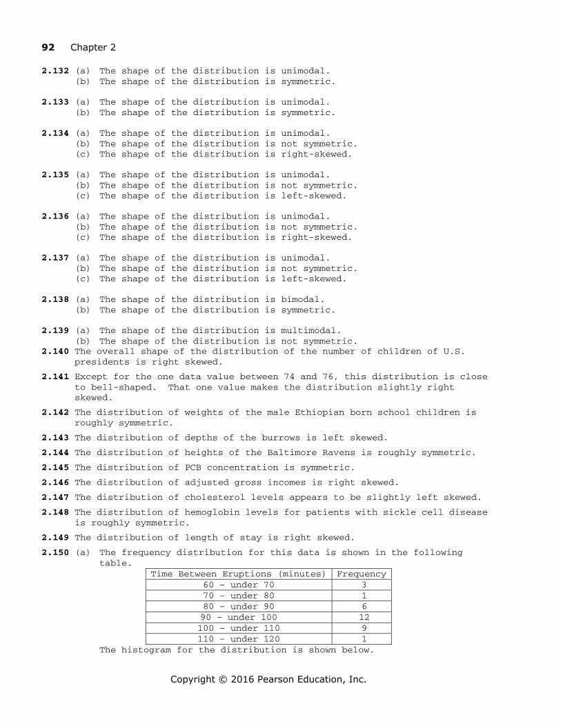
92 Chapter 2
Copyright © 2016 Pearson Education, Inc.
2.132 (a) The shape of the distribution is unimodal. (b) The shape of the distribution is symmetric. 2.133 (a) The shape of the distribution is unimodal. (b) The shape of the distribution is symmetric. 2.134 (a) The shape of the distribution is unimodal. (b) The shape of the distribution is not symmetric. (c) The shape of the distribution is right-skewed. 2.135 (a) The shape of the distribution is unimodal. (b) The shape of the distribution is not symmetric. (c) The shape of the distribution is left-skewed. 2.136 (a) The shape of the distribution is unimodal. (b) The shape of the distribution is not symmetric. (c) The shape of the distribution is right-skewed. 2.137 (a) The shape of the distribution is unimodal. (b) The shape of the distribution is not symmetric. (c) The shape of the distribution is left-skewed. 2.138 (a) The shape of the distribution is bimodal. (b) The shape of the distribution is symmetric. 2.139 (a) The shape of the distribution is multimodal. (b) The shape of the distribution is not symmetric. 2.140 The overall shape of the distribution of the number of children of U.S.
presidents is right skewed.
2.141 Except for the one data value between 74 and 76, this distribution is close to bell-shaped. That one value makes the distribution slightly right skewed.
2.142 The distribution of weights of the male Ethiopian born school children is roughly symmetric.
2.143 The distribution of depths of the burrows is left skewed.
2.144 The distribution of heights of the Baltimore Ravens is roughly symmetric.
2.145 The distribution of PCB concentration is symmetric.
2.146 The distribution of adjusted gross incomes is right skewed.
2.147 The distribution of cholesterol levels appears to be slightly left skewed.
2.148 The distribution of hemoglobin levels for patients with sickle cell disease is roughly symmetric.
2.149 The distribution of length of stay is right skewed.
2.150 (a) The frequency distribution for this data is shown in the following table.
Time Between Eruptions (minutes) Frequency60 – under 70 3 70 – under 80 1 80 – under 90 6 90 – under 100 12 100 – under 110 9 110 – under 120 1
The histogram for the distribution is shown below.

Section 2.4 93
Copyright © 2016 Pearson Education, Inc.
1 201 1 01 0090807060
1 2
1 0
8
6
4
2
0
TIME
Freq
uenc
y
(b) This distribution is unimodal.
(c) This distribution is not symmetric.
(d) This distribution is left skewed.
2.151 (a) The distributions for Year 1 and Year 2 are both unimodal. (b) Both distributions are not symmetric. (c) Both distributions are right skewed. (d) The distribution for Year 1 has a longer right tail indicating more
variation than the distribution for Year 2. They are also not centered in the same place.
2.152 (a) After entering the data from the WeissStats Resource Site, in
Minitab, select Graph <Histogram, select Simple and click OK. Double click on PUPS to enter PUPS in the Graph variables box and click OK. Our result is as follows. Results may vary depending on the type of technology used and graph obtained.
The overall shape of the distribution is unimodal and symmetric.
2.153 (a) After entering the data from the WeissStats Resource Site, in
Minitab, select Graph < Histogram, select Simple and click OK. Double click on LENGTH to enter LENGTH in the Graph variables box and click OK. Our result is as follows. Results may vary depending on the type of technology used and graph obtained.
PUPS
Freq
uenc
y
1210864
18
16
14
12
10
8
6
4
2
0
Histogram of PUPS

94 Chapter 2
Copyright © 2016 Pearson Education, Inc.
4503753002251 5075
70
60
50
40
30
20
1 0
0
LENGTH
Freq
uenc
y
The distribution of LENGTH is unimodal and not symmetric.
(b) The distribution is right skewed.
2.154 (a) In Exercise 2.108, we used Minitab to obtain a stem-and-leaf diagram using 5 lines per stem. That diagram is shown below
Stem-and-leaf of PERCENT N = 51 Leaf Unit = 1.0 3 8 001
10 8 2222333 18 8 44444555 (8) 8 66777777
25 8 888889999 16 9 00000000011111 2 9 22
The overall shape of this distribution is unimodal and not symmetric.
(b) The distribution is left skewed.
2.155 (a) In Exercise 2.109, we used Minitab to obtain a stem-and-leaf diagram using 2 lines per stem. That diagram is shown below.
Stem-and-leaf of PERCENT N = 51 Leaf Unit = 1.0
2 1 79 14 2 011223334444 (20) 2 55555566666777778999 17 3 00011122234 6 3 56668 1 4 1 4 9
The overall shape of this distribution is unimodal and roughly symmetric.
2.156 (a) After entering the data in Minitab, select Graph < Dotplot, select Simple in the One Y row, and click OK. Double click on TEMP to enter TEMP in the Graph variables box and click OK. Our result is as follows. Results may vary depending on the type of technology used and graph obtained.

Section 2.4 95
Copyright © 2016 Pearson Education, Inc.
TEMP99.298.898.498.097.697.296.8
Dotplot of TEMP
The overall distribution of temperatures is roughly unimodal and roughly symmetric.
2.157 (a) After entering the data from the WeissStats Resource Site, in
Minitab, select Graph < Histogram, select Simple and click OK. Double click on LENGTH to enter LENGTH in the Graph variables box and click OK. Our result is as follows. Results may vary depending on the type of technology used and graph obtained.
212019181716
30
25
20
15
10
5
0
LENGTH
Freq
uenc
y
Histogram of LENGTH
The distribution of LENGTH is approximately unimodal and symmetric.
2.158 Class Project. The precise answers to this exercise will vary from class to class.
2.159 The precise answers to this exercise will vary from class to class or individual to individual. Thus your results will likely differ from our results shown below.
(a) We obtained 50 random digits from a table of random numbers. The digits were
4 5 4 6 8 9 9 7 7 2 2 2 9 3 0 3 4 0 0 8 8 4 4 5 3
9 2 4 8 9 6 3 0 1 1 0 9 2 8 1 3 9 2 5 8 1 8 9 2 2
(b) Since each digit is equally likely in the random number table, we expect that the distribution would look roughly uniform.
(c) Using single value classes, the frequency distribution is given by the following table. The relative frequency histogram is shown below.
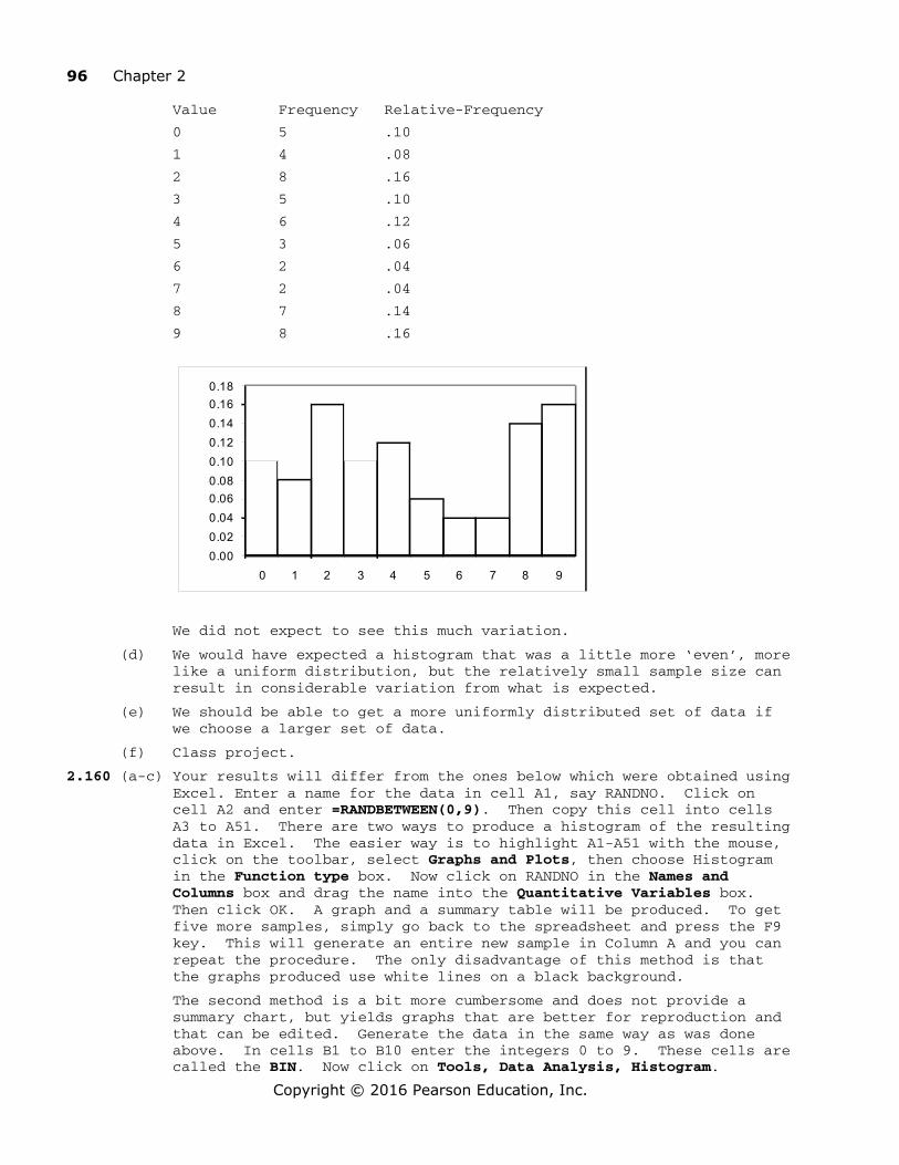
96 Chapter 2
Copyright © 2016 Pearson Education, Inc.
Value Frequency Relative-Frequency
0 5 .10
1 4 .08
2 8 .16
3 5 .10
4 6 .12
5 3 .06
6 2 .04
7 2 .04
8 7 .14
9 8 .16
We did not expect to see this much variation.
(d) We would have expected a histogram that was a little more ‘even’, more like a uniform distribution, but the relatively small sample size can result in considerable variation from what is expected.
(e) We should be able to get a more uniformly distributed set of data if we choose a larger set of data.
(f) Class project.
2.160 (a-c) Your results will differ from the ones below which were obtained using Excel. Enter a name for the data in cell A1, say RANDNO. Click on cell A2 and enter =RANDBETWEEN(0,9). Then copy this cell into cells A3 to A51. There are two ways to produce a histogram of the resulting data in Excel. The easier way is to highlight A1-A51 with the mouse, click on the toolbar, select Graphs and Plots, then choose Histogram in the Function type box. Now click on RANDNO in the Names and Columns box and drag the name into the Quantitative Variables box. Then click OK. A graph and a summary table will be produced. To get five more samples, simply go back to the spreadsheet and press the F9 key. This will generate an entire new sample in Column A and you can repeat the procedure. The only disadvantage of this method is that the graphs produced use white lines on a black background.
The second method is a bit more cumbersome and does not provide a summary chart, but yields graphs that are better for reproduction and that can be edited. Generate the data in the same way as was done above. In cells B1 to B10 enter the integers 0 to 9. These cells are called the BIN. Now click on Tools, Data Analysis, Histogram.
0.000.020.040.060.080.100.120.140.160.18
0 1 2 3 4 5 6 7 8 9

Section 2.4 97
Copyright © 2016 Pearson Education, Inc.
(If Data Analysis is not in the Tools menu, you will have to add it from the original CD.) Click on the Input box and highlight cells A2-A51 with the mouse, then click on the Bin box and highlight cells B1-B10. Finally click on the Output box and enter C1. This will give you a frequency table in columns C and D. Now enter the integers 0 to 9 as text in cells E2 to E11 by entering each digit preceded by a single quote mark, i.e., ‘0, ‘1, etc. In cell F2, enter =D2, and copy this cell into F3 through F11. Now highlight the data in columns E and F with the mouse and click the chart icon, pick the Column graph type, pick the first sub-type, click on the Next button twice, enter any titles desired, remove the legend, and then click on the Next button and then the Finish button. The graph will appear on the spreadsheet as a bar chart with spaces between the bars. Use the mouse to point to any one of the bars and click with the right mouse button. Choose Format Data Series. Click on the Options tab and change the Gap Width to zero, and click OK. Repeat this sequence to produce additional histograms, but use different cells.
[If you would like to avoid repeating most of the above steps, click near the border of the graph and copy the graph to the Clipboard, then go to Microsoft Word or other word processor, and click on Edit on the Toolbar and Paste Special. Highlight Microsoft Excel Chart Object, and click OK. The graphs can be resized in the word processor if necessary. Now go back to Excel and hit the F9 key. This will produce a completely new set of random numbers. Click on Tools, Data Analysis, Histogram, leave all the boxes as they are and click OK. Then click OK to overwrite existing data. A new table will be created and the existing histogram will be updated automatically. We used this process for the following histograms.]
(d) These shapes are about what we expected.
(e) The relative frequency histograms for six samples of digits of size
1000 were obtained using Minitab. Choose Calc < Random Data < Integer..., type 1000 in the Generate rows of data test box, click in
the Store in column(s) text box and type C1 C2 C3 C4 C5 C6, click in the Minimum value text box and type 0, type in the Maximum value text
box and type 9 and click OK. Then choose Graph < Histogram, select the Simple version and click OK, enter C1 C2 C3 C4 C5 C6 in the Graph

98 Chapter 2
Copyright © 2016 Pearson Education, Inc.
C3
Freq
uenc
y
86420
120
100
80
60
40
20
0
Histogram of C3
C4
Freq
uenc
y
86420
120
100
80
60
40
20
0
Histogram of C4
C6
Freq
uenc
y
86420
120
100
80
60
40
20
0
Histogram of C6
C5
Freq
uenc
y
86420
120
100
80
60
40
20
0
Histogram of C5
C2
Freq
uenc
y
86420
120
100
80
60
40
20
0
Histogram of C2
variables text box, C2 in the Graph 2 text box un x, and so on for C3 through C6. Click on the Multiple Graphs button. Click on the On separate graphs button, and check the boxes for Same Y and Same X, including same bins. Click OK and click OK. The following graphs resulted.
The histograms for samples of size 1000 are much closer to the rectangular distribution we expected than are the ones for samples of size 50.
C1
Freq
uenc
y
86420
120
100
80
60
40
20
0
Histogram of C1

Section 2.5 99
Copyright © 2016 Pearson Education, Inc.
C1
Perc
ent
3210-1-2-3
8
7
6
5
4
3
2
1
0
Histogram of C1
2.161 (a) Your result will differ from, but be similar to, the one below which
was obtained using Minitab. Choose Calc < Random Data < Normal..., type 3000 in the Generate rows of data text box, click in the Store in column(s) text box and type C1, and click OK.
(b) Then choose Graph < Histogram, choose the Simple version, click OK, enter C1 in the Graph variables text box, click on the Scale button and then on the Y-Scale Type tab. Check the Percent box and click OK twice.
(c) The histogram in part (b) has the bell, unimodal and symmetric distribution. The sample of 3000 is representative of the population from which the sample was taken.
Section 2.5
2.162 Graphs are sometimes constructed in ways that cause them to be misleading.
2.163 (a) A truncated graph is one for which the vertical axis starts at a value other than its natural starting point, usually zero.
(b) A legitimate motivation for truncating the axis of a graph is to place the emphasis on the ups and downs of the distribution rather than on the actual height of the graph.
(c) To truncate a graph and avoid the possibility of misinterpretation, one should start the axis at zero and put slashes in the axis to indicate that part of the axis is missing.
2.164 Answers will vary.
2.165 (a) A large lower portion of the graph is eliminated. When this is done, differences between district and national averages appear greater than in the original figure.
(b) Even more of the graph is eliminated. Differences between district and national averages appear even greater than in part (a).
(c) The truncated graphs give the misleading impression that, in 2013, the district average is much greater relative to the national average than it actually is.
2.166 (a) A break is shown in the first bar on the left to warn the reader that part of the first bar itself has been removed.
(b) It was necessary to construct the graph with a broken bar to let the reader know that the first bar is actually much taller than it appears. If the true height of the first bar were presented, but without the break, the height would span most of an entire page. This
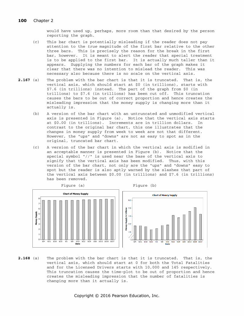
100 Chapter 2
Copyright © 2016 Pearson Education, Inc.
would have used up, perhaps, more room than that desired by the person reporting the graph.
(c) This bar chart is potentially misleading if the reader does not pay attention to the true magnitude of the first bar relative to the other three bars. This is precisely the reason for the break in the first bar, however. It is meant to alert the reader that special treatment is to be applied to the first bar. It is actually much taller than it appears. Supplying the numbers for each bar of the graph makes it clear that there was no intention to mislead the reader. This was necessary also because there is no scale on the vertical axis.
2.167 (a) The problem with the bar chart is that it is truncated. That is, the vertical axis, which should start at $0 (in trillions), starts with $7.6 (in trillions) instead. The part of the graph from $0 (in trillions) to $7.6 (in trillions) has been cut off. This truncation causes the bars to be out of correct proportion and hence creates the misleading impression that the money supply is changing more than it actually is.
(b) A version of the bar chart with an untruncated and unmodified vertical axis is presented in Figure (a). Notice that the vertical axis starts at $0.00 (in trillions). Increments are in trillion dollars. In contrast to the original bar chart, this one illustrates that the changes in money supply from week to week are not that different. However, the "ups" and "downs" are not as easy to spot as in the original, truncated bar chart.
(c) A version of the bar chart in which the vertical axis is modified in an acceptable manner is presented in Figure (b). Notice that the special symbol "//" is used near the base of the vertical axis to signify that the vertical axis has been modified. Thus, with this version of the bar chart, not only are the "ups" and "downs" easy to spot but the reader is also aptly warned by the slashes that part of the vertical axis between $0.00 (in trillions) and $7.6 (in trillions) has been removed.
Figure (a) Figure (b)
10/2710/2010/1310/69/299/229/159/89/18/258/188/118/4
8
7
6
5
4
3
2
1
0
Date
Mon
ey S
uppl
y
Chart of Money Supply
2.168 (a) The problem with the bar chart is that it is truncated. That is, the vertical axis, which should start at 0 for both the Total Fatalities and for the Licensed Drivers starts with 10,000 and 145 respectively. This truncation causes the time-plot to be out of proportion and hence creates the misleading impression that the number of fatalities is changing more than it actually is.
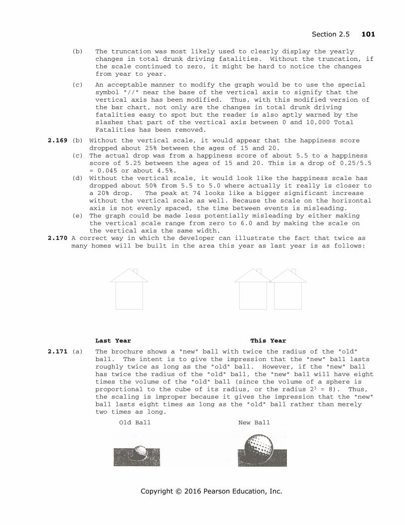
Section 2.5 101
Copyright © 2016 Pearson Education, Inc.
(b) The truncation was most likely used to clearly display the yearly changes in total drunk driving fatalities. Without the truncation, if the scale continued to zero, it might be hard to notice the changes from year to year.
(c) An acceptable manner to modify the graph would be to use the special symbol "//" near the base of the vertical axis to signify that the vertical axis has been modified. Thus, with this modified version of the bar chart, not only are the changes in total drunk driving fatalities easy to spot but the reader is also aptly warned by the slashes that part of the vertical axis between 0 and 10,000 Total Fatalities has been removed.
2.169 (b) Without the vertical scale, it would appear that the happiness score dropped about 25% between the ages of 15 and 20.
(c) The actual drop was from a happiness score of about 5.5 to a happiness score of 5.25 between the ages of 15 and 20. This is a drop of 0.25/5.5 = 0.045 or about 4.5%.
(d) Without the vertical scale, it would look like the happiness scale has dropped about 50% from 5.5 to 5.0 where actually it really is closer to a 20% drop. The peak at 74 looks like a bigger significant increase without the vertical scale as well. Because the scale on the horizontal axis is not evenly spaced, the time between events is misleading.
(e) The graph could be made less potentially misleading by either making the vertical scale range from zero to 6.0 and by making the scale on the vertical axis the same width.
2.170 A correct way in which the developer can illustrate the fact that twice as many homes will be built in the area this year as last year is as follows:
Last Year This Year
2.171 (a) The brochure shows a "new" ball with twice the radius of the "old" ball. The intent is to give the impression that the "new" ball lasts roughly twice as long as the "old" ball. However, if the "new" ball has twice the radius of the "old" ball, the "new" ball will have eight times the volume of the "old" ball (since the volume of a sphere is proportional to the cube of its radius, or the radius 23 = 8). Thus, the scaling is improper because it gives the impression that the "new" ball lasts eight times as long as the "old" ball rather than merely two times as long.
Old Ball New Ball

102 Chapter 2
Copyright © 2016 Pearson Education, Inc.
(b) One possible way for the manufacturer to illustrate the fact that the "new" ball lasts twice as long as the "old" ball is to present pictures of two balls, side by side, each of the same magnitude as the picture of the "old" ball and to label this set of two balls "new ball". This will illustrate the point that a purchaser will be getting twice as much for the money.
Old Ball New Ball
Review Problems For Chapter 2
1. (a) A variable is a characteristic that varies from one person or thing to another.
(b) Variables are quantitative or qualitative.
(c) Quantitative variables can be discrete or continuous.
2. (d) Data are values of a variable.
(e) The data type is determined by the type of variable being observed.
3. A frequency distribution of qualitative data is a table that lists the distinct values of data and their frequencies. It is useful to organize the data and make it easier to understand. A relative-frequency distribution of qualitative data is a table that lists the distinct values of data and a ratio of the class frequency to the total number of observations, which is called the relative frequency.
4. For both quantitative and qualitative data, the frequency and relative-frequency distributions list the values of the distinct classes and their frequencies and relative frequencies. For single value grouping of quantitative data, it is the same as the distinct classes for qualitative data. For class limit and cutpoint grouping in quantitative data, we create groups that form distinct classes similar to qualitative data.
5. The two main types of graphical displays for qualitative data are the bar chart and the pie chart.
6. The bars do not abut in a bar chart because there is not any continuity between the categories. Also, this differentiates them from histograms.
7. Answers will vary. One advantage of pie charts is that it shows the proportion of each class to the total. One advantage of bar charts is that it emphasizes each individual class in relation to each other. One disadvantage of pie charts is that if there are too many classes, the chart becomes confusing. Also, if a class is really small relative to the total, it is hard to see the class in a pie chart.
8. Single value grouping is appropriate when the data are discrete with relatively few distinct observations.

Review Problems 103
Copyright © 2016 Pearson Education, Inc.
9. (a) The second class would have lower and upper limits of 9 and 14. The class mark of this class would be the average of these limits and equal 11.5.
(b) The third class would have lower and upper limits of 15 and 20.
(c) The fourth class would have lower and upper limits of 21 and 26. This class would contain an observation of 23.
10. (a) If the width of the class is 5, then the class limits will be four whole numbers apart. Also, the average of the two class limits is the class mark of 8. Therefore, the upper and lower class limits must be two whole numbers above and below the number 8. The lower and upper class limits of the first class are 6 and 10.
(b) The second class will have lower and upper class limits of 11 and 15. Therefore, the class mark will be the average of these two limits and equal 13.
(c) The third class will have lower and upper class limits of 16 and 20.
(d) The fourth class has limits of 21 and 25, the fifth class has limits of 26 and 30. Therefore, the fifth class would contain an observation of 28.
11. (a) The common class width is the distance between consecutive cutpoints, which is 15 - 5 = 10.
(b) The midpoint of the second class is halfway between the cutpoints 15 and 25, and is therefore 20.
(c) The sequence of the lower cutpoints is 5, 15, 25, 35, 45, ... Therefore, the lower and upper cutpoints of the third class are 25 and 35.
(d) Since the third class has lower and upper cutpoints of 25 and 35, an observation of 32.4 would belong to this class.
12. (a) The midpoint is halfway between the cutpoints. Since the class width is 8, 10 is halfway between 6 and 14.
(b) The class width is also the distance between consecutive midpoints. Therefore, the second midpoint is at 10 + 8 = 18.
(c) The sequence of cutpoints is 6, 14, 22, 30, 38, ... Therefore the lower and upper cutpoints of the third class are 22 and 30.
(d) An observation of 22 would go into the third class since that class contains data greater than or equal to 22 and strictly less than 30.
13. (a) If lower class limits are used to label the horizontal axis, the bars are placed between the lower class limit of one class and the lower class limit of the next class.
(b) If lower cutpoints are used to label the horizontal axis, the bars are placed between the lower cutpoint of one class and the lower cutpoint of the next class.
(c) If class marks are used to label the horizontal axis, the bars are placed directly above and centered over the class mark for that class.
(d) If midpoints are used to label the horizontal axis, the bars are placed directly above and centered over the midpoint for that class.

104 Chapter 2
Copyright © 2016 Pearson Education, Inc.
14.(a)Bell-shaped (b)Triangular (c) Reverse J shape (d)Uniform
15. Answers will vary but here is one possibility.
16. (a) The distribution of the large simple random sample will reflect the distribution of the population, so it would be left-skewed as well.
(b) No. The randomness in the samples will almost certainly produce different sets of observations resulting in shapes that are not identical.
(c) Yes. We would expect both of the simple random samples to reflect the shape of the population and be left-skewed.
17. (a) The first column ranks the hydroelectric plants. Thus, it consists of quantitative, discrete data.
(b) The fourth column provides measurements of capacity. Thus, it consists of quantitative, continuous data.
(c) The third column provides nonnumerical information. Thus, it consists of qualitative data.
18. (a) A single value frequency histogram for the prices of DVD players would be identical to the dotplot in example 2.16 because the classes would be 197 through 224 and the height for each bar in the frequency histogram would reflect the number of dots above each observation in the dotplot.
(b) No. The frequency histogram with cutpoint or class limit grouping would combine some of the single values together which would change the frequencies and the heights of the bars corresponding to those classes.
19. (a) The first class to construct is 40-44. Since all classes are to be of equal width, and the second class begins with 45, we know that the width of all classes is 45 - 40 = 5. All of the classes are presented in column 1 of the grouped-data table in the figure below. The last class to construct does not go beyond 65-69, since the largest single data value is 69. The sum of the relative frequency column is 0.999 due to rounding.

Review Problems 105
Copyright © 2016 Pearson Education, Inc.
Age at Inauguration
Frequency
Relative Frequency
Class Mark
40-44 2 0.045 42
45-49 7 0.159 47
50-54 13 0.295 52
55-59 12 0.273 57
60-64 7 0.159 62
65-69 3 0.068 67
44 0.999
(b) By averaging the lower and upper limits for each class, we arrive at the class mark for each class. The class marks for all classes are presented in column 4.
(c) Having established the classes, we tally the ages into their respective classes. These results are presented in column 2, which lists the frequencies. Dividing each frequency by the total number of observations, which is 44, results in each class's relative frequency. The relative frequencies for all classes are presented in column 3.
(d) The frequency histogram presented below is constructed using the frequency distribution presented above; i.e., columns 1 and 2. Notice that the lower cutpoints of column 1 are used to label the horizontal axis of the frequency histogram. Suitable candidates for vertical-axis units in the frequency histogram are the even integers within the range 2 through 14, since these are representative of the magnitude and spread of the frequencies presented in column 2. The height of each bar in the frequency histogram matches the respective frequency in column 2.
70656055504540
14
12
10
8
6
4
2
0
AGE
Freq
uenc
y
Histogram of AGE
(e) The shape of the inauguration ages is unimodal and symmetric.
20. The horizontal axis of this dotplot displays a range of possible ages for the 44 Presidents of the United States. To complete the dotplot, we go through the data set and record each age by placing a dot over the appropriate value on the horizontal axis.

106 Chapter 2
Copyright © 2016 Pearson Education, Inc.
68646056524844AGE
Age at Inauguration for first 44 Presidents
21. (a) Using one line per stem in constructing the ordered stem-and-leaf diagram means vertically listing the numbers comprising the stems once. The leaves are then placed with their respective stems in order. The ordered stem-and-leaf diagram using one line per stem is presented in the following figure.
4| 236677899 5| 0011112244444555566677778 6| 0111244589
(b) Using two lines per stem in constructing the ordered stem-and-leaf diagram means vertically listing the numbers comprising the stems twice. In turn, if the leaf is one of the digits 0 through 4, it is ordered and placed with the first of the two stem lines. If the leaf is one of the digits 5 through 9, it is ordered and placed with the second of the two stem lines. The ordered stem-and-leaf diagram using two lines per stem is presented in the following figure.
4| 23 4| 6677899 5| 0011112244444 5| 555566677778 6| 0111244 6| 589
(c) The stem-and-leaf diagram in part (b) corresponds to the frequency distribution of Problem 19.
22. (a) Using one line per stem in constructing the ordered stem-and-leaf diagram means vertically listing the numbers comprising the stems once. The leaves are then placed with their respective stems in order. The ordered stem-and-leaf diagram using one line per stem is presented in the following figure.
3| 4778 4| 0467 5| 446677778
6| 0
(b) Using two lines per stem in constructing the ordered stem-and-leaf diagram means vertically listing the numbers comprising the stems twice. In turn, if the leaf is one of the digits 0 through 4, it is ordered and placed with the first of the two stem lines. If the leaf is one of the digits 5 through 9, it is ordered and placed with the second of the two stem lines. The ordered stem-and-leaf diagram using two lines per stem is presented in the following figure.
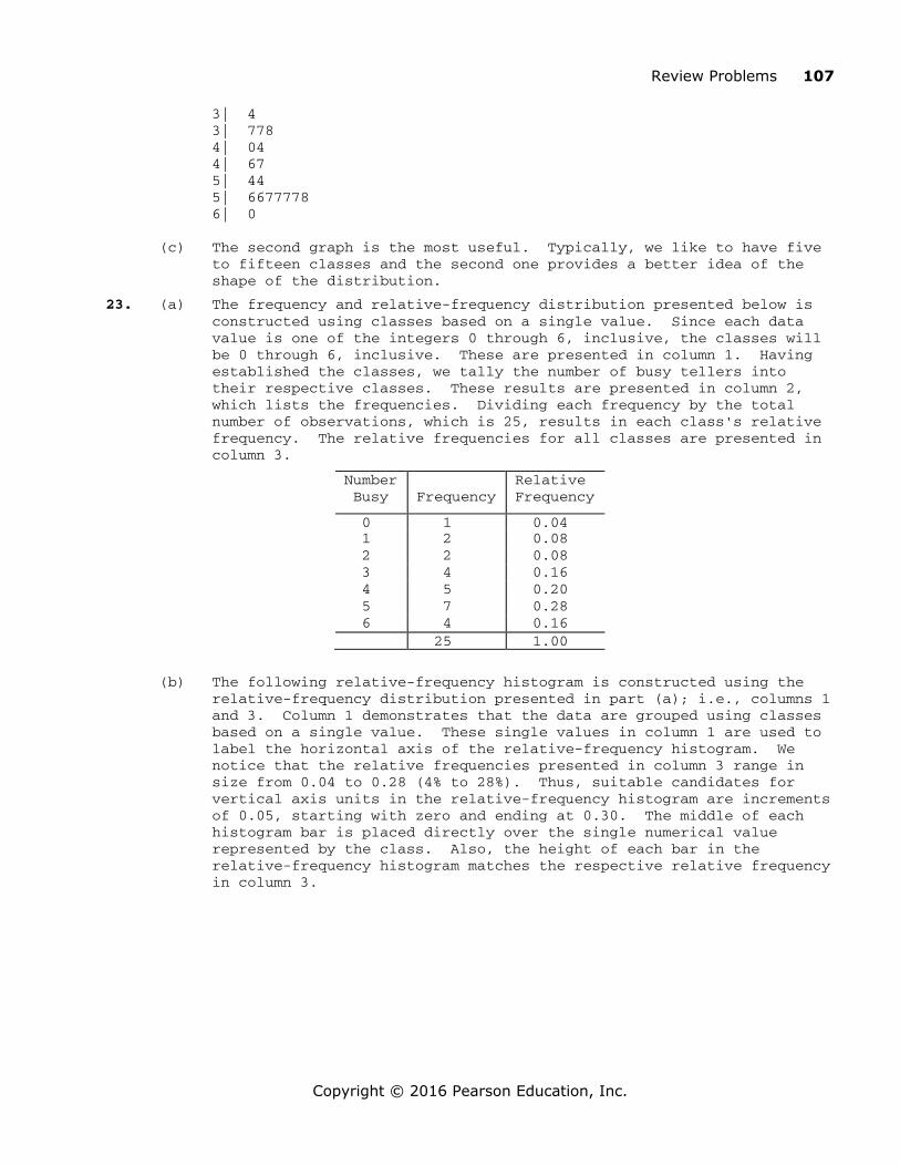
Review Problems 107
Copyright © 2016 Pearson Education, Inc.
3| 4 3| 778 4| 04 4| 67 5| 44 5| 6677778 6| 0
(c) The second graph is the most useful. Typically, we like to have five to fifteen classes and the second one provides a better idea of the shape of the distribution.
23. (a) The frequency and relative-frequency distribution presented below is constructed using classes based on a single value. Since each data value is one of the integers 0 through 6, inclusive, the classes will be 0 through 6, inclusive. These are presented in column 1. Having established the classes, we tally the number of busy tellers into their respective classes. These results are presented in column 2, which lists the frequencies. Dividing each frequency by the total number of observations, which is 25, results in each class's relative frequency. The relative frequencies for all classes are presented in column 3.
Number Busy
Frequency
Relative Frequency
0 1 0.04 1 2 0.08 2 2 0.08 3 4 0.16 4 5 0.20 5 7 0.28 6 4 0.16 25 1.00
(b) The following relative-frequency histogram is constructed using the relative-frequency distribution presented in part (a); i.e., columns 1 and 3. Column 1 demonstrates that the data are grouped using classes based on a single value. These single values in column 1 are used to label the horizontal axis of the relative-frequency histogram. We notice that the relative frequencies presented in column 3 range in size from 0.04 to 0.28 (4% to 28%). Thus, suitable candidates for vertical axis units in the relative-frequency histogram are increments of 0.05, starting with zero and ending at 0.30. The middle of each histogram bar is placed directly over the single numerical value represented by the class. Also, the height of each bar in the relative-frequency histogram matches the respective relative frequency in column 3.
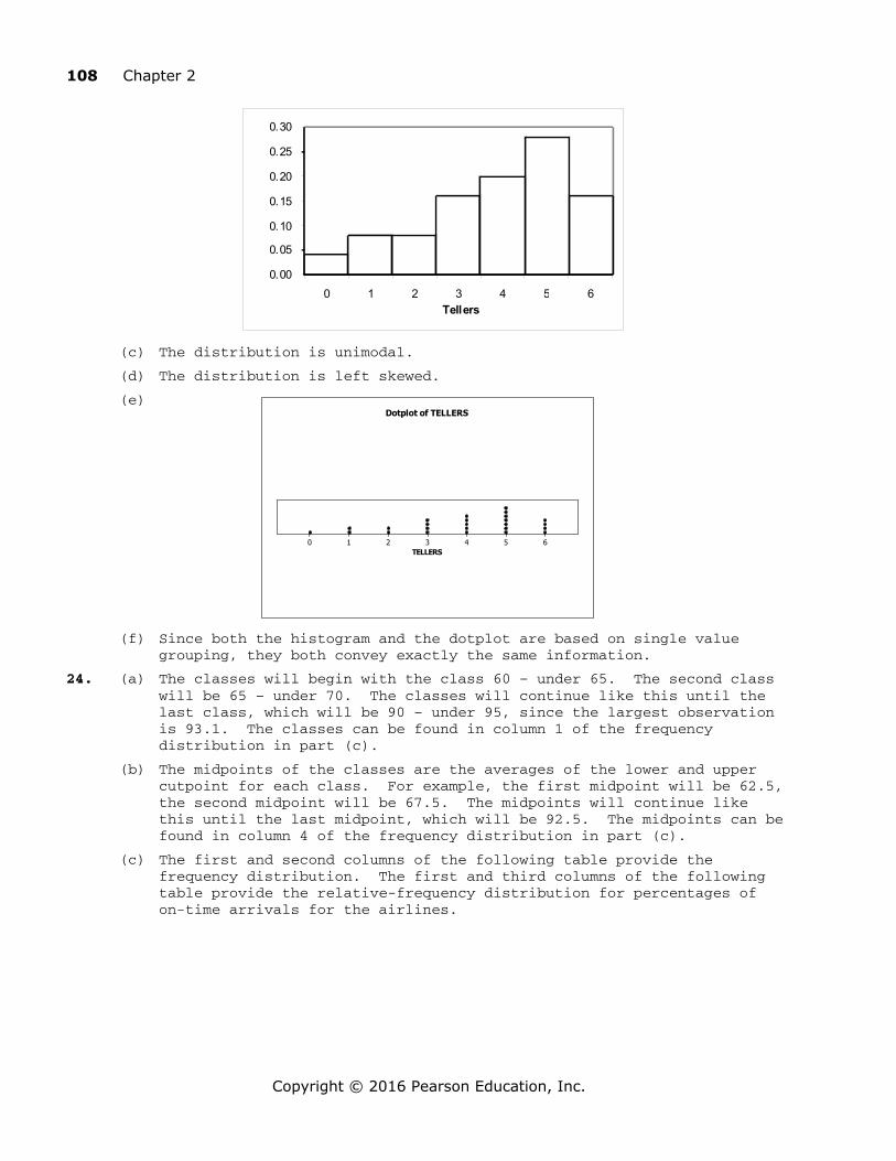
108 Chapter 2
Copyright © 2016 Pearson Education, Inc.
0.00
0.05
0.10
0.15
0.20
0.25
0.30
0 1 2 3 4 5 6Tellers
TELLERS6543210
Dotplot of TELLERS
(c) The distribution is unimodal.
(d) The distribution is left skewed.
(e)
(f) Since both the histogram and the dotplot are based on single value grouping, they both convey exactly the same information.
24. (a) The classes will begin with the class 60 – under 65. The second class will be 65 – under 70. The classes will continue like this until the last class, which will be 90 – under 95, since the largest observation is 93.1. The classes can be found in column 1 of the frequency distribution in part (c).
(b) The midpoints of the classes are the averages of the lower and upper cutpoint for each class. For example, the first midpoint will be 62.5, the second midpoint will be 67.5. The midpoints will continue like this until the last midpoint, which will be 92.5. The midpoints can be found in column 4 of the frequency distribution in part (c).
(c) The first and second columns of the following table provide the frequency distribution. The first and third columns of the following table provide the relative-frequency distribution for percentages of on-time arrivals for the airlines.
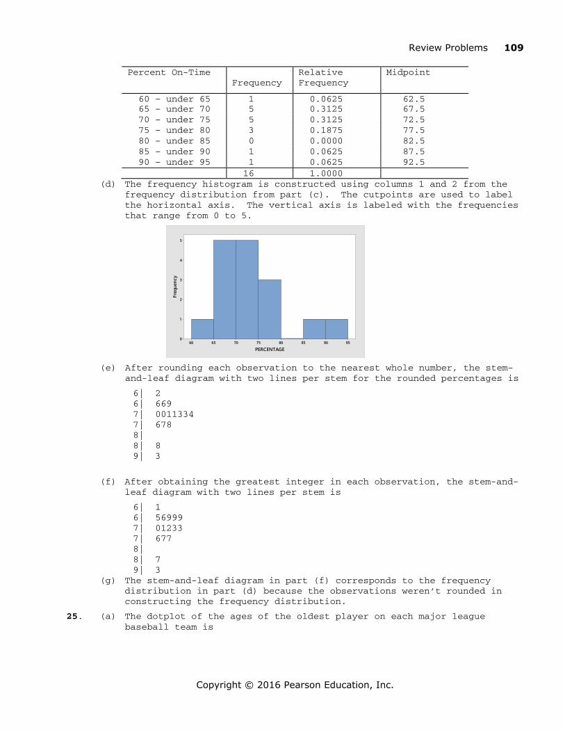
Review Problems 109
Copyright © 2016 Pearson Education, Inc.
Percent On-Time
Frequency
Relative Frequency
Midpoint
60 – under 65 1 0.0625 62.5 65 – under 70 5 0.3125 67.5 70 – under 75 5 0.3125 72.5 75 – under 80 3 0.1875 77.5 80 – under 85 0 0.0000 82.5 85 – under 90 1 0.0625 87.5 90 – under 95 1 0.0625 92.5 16 1.0000
(d) The frequency histogram is constructed using columns 1 and 2 from the frequency distribution from part (c). The cutpoints are used to label the horizontal axis. The vertical axis is labeled with the frequencies that range from 0 to 5.
9590858075706560
5
4
3
2
1
0
PERCENTAGE
Freq
uenc
y
(e) After rounding each observation to the nearest whole number, the stem-
and-leaf diagram with two lines per stem for the rounded percentages is
6| 2 6| 669 7| 0011334 7| 678 8| 8| 8 9| 3
(f) After obtaining the greatest integer in each observation, the stem-and-leaf diagram with two lines per stem is
6| 1 6| 56999 7| 01233 7| 677 8| 8| 7 9| 3
(g) The stem-and-leaf diagram in part (f) corresponds to the frequency distribution in part (d) because the observations weren’t rounded in constructing the frequency distribution.
25. (a) The dotplot of the ages of the oldest player on each major league baseball team is

110 Chapter 2
Copyright © 2016 Pearson Education, Inc.
AGES46444240383634
Dotplot of AGES
(b) The overall shape of the distribution of ages is bimodal and roughly symmetric.
26. (a) The classes are the types of evidence and are presented in column 1. The frequency distribution of the champions is presented in column 2. Dividing each frequency by the total number of submissions, which is 3436, results in each class's relative frequency. The relative frequency distribution is presented in column 3.
Evidence Type Frequency Relative Frequency Firearm 289 0.084
Magazine 161 0.047
Live Cartridge 2727 0.794
Spent Cartridge 259 0.075
3436 1.000
(b) We multiply each of the relative frequencies by 360 degrees to obtain the portion of the pie represented by each evidence type. The result is
FirearmMagazineLive cartridgeSpent cartridge casing
CategorySpent cartridge casing7.5%
Live cartridge79.4%
Magazine4.7%
Firearm8.4%
Pie Chart of EVIDENCE TYPE
(c) We use the bar chart to show the relative frequency with which each EVIDENCE TYPE occurs. The result is

Review Problems 111
Copyright © 2016 Pearson Education, Inc.
Spent cartridge casingLive cartridgeMagazineFirearm
80
70
60
50
40
30
20
1 0
0
EVIDENCE
Perc
ent o
f FRE
QUEN
CY
Percent within all data.
Evidence Type
(d) The most common type of evidence type submitted to crime labs is a live
cartridge which was the type submitted 79.4% of the time.
27. (a) The population consists of the states in the United States. The variable is the division.
(b) The frequency and relative frequency distribution for Region is shown below.
Region Frequency
Relative Frequency
East North Central 5 0.10
East South Central 4 0.08
Middle Atlantic 3 0.06
Mountain 8 0.16
New England 6 0.12
Pacific 5 0.10
South Atlantic 8 0.16
West North Central 7 0.14
West South Central 4 0.08
50 1.000
(c) The pie chart for Region is shown below.
MTNSACWNCNEDENCPACESCWSCMAC
CategoryMAC6.0%
WSC8.0%
ESC8.0%
PAC10.0%
ENC10.0%
NED12.0%
WNC14.0%
SAC16.0%
MTN16.0%
Pie Chart of DIVISION
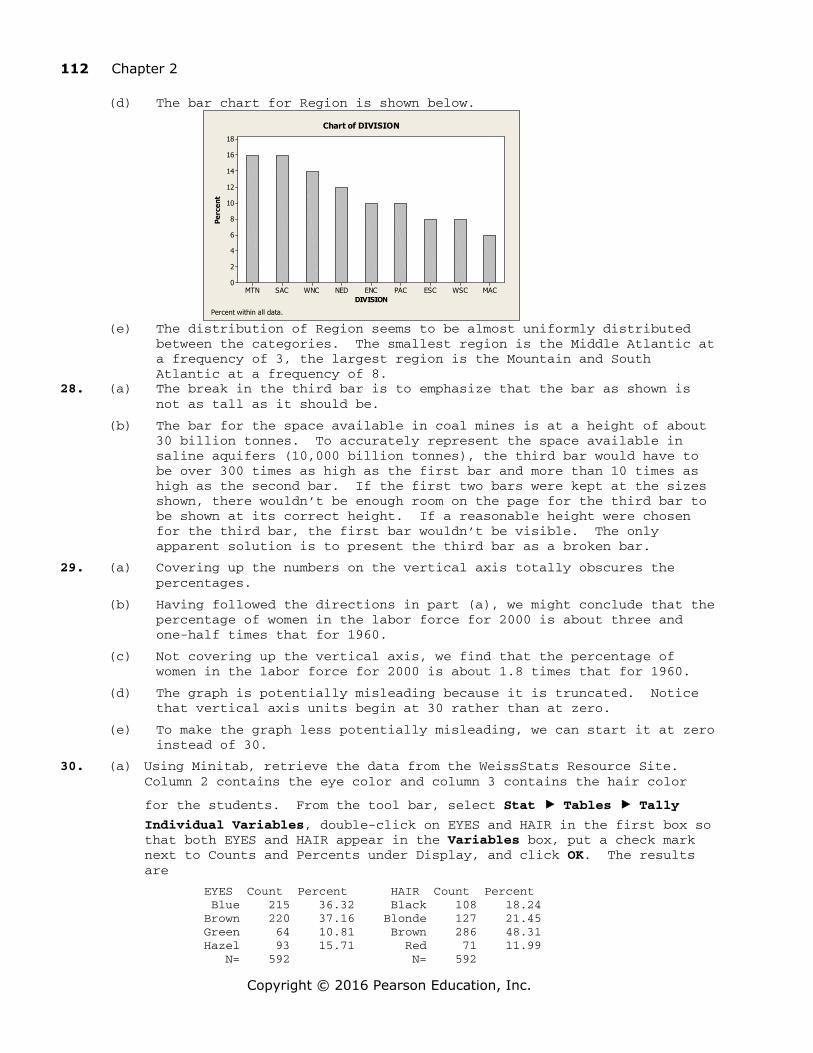
112 Chapter 2
Copyright © 2016 Pearson Education, Inc.
(d) The bar chart for Region is shown below.
MACWSCESCPACENCNEDWNCSACMTN
18
16
14
12
10
8
6
4
2
0
DIVISION
Perc
ent
Chart of DIVISION
Percent within all data. (e) The distribution of Region seems to be almost uniformly distributed
between the categories. The smallest region is the Middle Atlantic at a frequency of 3, the largest region is the Mountain and South Atlantic at a frequency of 8.
28. (a) The break in the third bar is to emphasize that the bar as shown is not as tall as it should be.
(b) The bar for the space available in coal mines is at a height of about 30 billion tonnes. To accurately represent the space available in saline aquifers (10,000 billion tonnes), the third bar would have to be over 300 times as high as the first bar and more than 10 times as high as the second bar. If the first two bars were kept at the sizes shown, there wouldn’t be enough room on the page for the third bar to be shown at its correct height. If a reasonable height were chosen for the third bar, the first bar wouldn’t be visible. The only apparent solution is to present the third bar as a broken bar.
29. (a) Covering up the numbers on the vertical axis totally obscures the percentages.
(b) Having followed the directions in part (a), we might conclude that the percentage of women in the labor force for 2000 is about three and one-half times that for 1960.
(c) Not covering up the vertical axis, we find that the percentage of women in the labor force for 2000 is about 1.8 times that for 1960.
(d) The graph is potentially misleading because it is truncated. Notice that vertical axis units begin at 30 rather than at zero.
(e) To make the graph less potentially misleading, we can start it at zero instead of 30.
30. (a) Using Minitab, retrieve the data from the WeissStats Resource Site. Column 2 contains the eye color and column 3 contains the hair color
for the students. From the tool bar, select Stat < Tables < Tally Individual Variables, double-click on EYES and HAIR in the first box so that both EYES and HAIR appear in the Variables box, put a check mark next to Counts and Percents under Display, and click OK. The results are
EYES Count Percent HAIR Count Percent Blue 215 36.32 Black 108 18.24 Brown 220 37.16 Blonde 127 21.45 Green 64 10.81 Brown 286 48.31 Hazel 93 15.71 Red 71 11.99 N= 592 N= 592
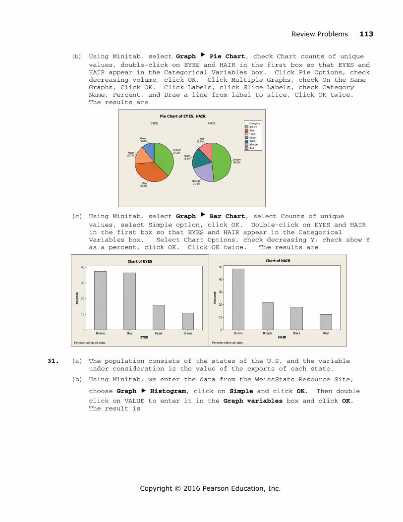
Review Problems 113
Copyright © 2016 Pearson Education, Inc.
(b) Using Minitab, select Graph < Pie Chart, check Chart counts of unique values, double-click on EYES and HAIR in the first box so that EYES and HAIR appear in the Categorical Variables box. Click Pie Options, check decreasing volume, click OK. Click Multiple Graphs, check On the Same Graphs, Click OK. Click Labels, click Slice Labels, check Category Name, Percent, and Draw a line from label to slice, Click OK twice. The results are
EYES HAIRBrownBlueHazelGreenBlackBlondeRed
Category
Green10.8%
Hazel15.7%
Blue36.3%
Brown37.2%
Red12.0%
Black18.2%
Blonde21.5%
Brown48.3%
Pie Chart of EYES, HAIR
(c) Using Minitab, select Graph < Bar Chart, select Counts of unique values, select Simple option, click OK. Double-click on EYES and HAIR in the first box so that EYES and HAIR appear in the Categorical Variables box. Select Chart Options, check decreasing Y, check show Y as a percent, click OK. Click OK twice. The results are
GreenHazelBlueBrown
40
30
20
10
0
EYES
Perc
ent
Chart of EYES
Percent within all data.
RedBlackBlondeBrown
50
40
30
20
10
0
HAIR
Perc
ent
Chart of HAIR
Percent within all data.
31. (a) The population consists of the states of the U.S. and the variable under consideration is the value of the exports of each state.
(b) Using Minitab, we enter the data from the WeissStats Resource Site,
choose Graph < Histogram, click on Simple and click OK. Then double click on VALUE to enter it in the Graph variables box and click OK. The result is
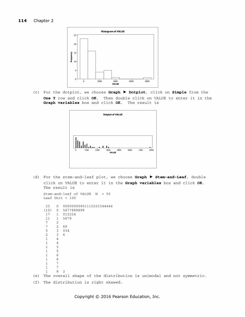
114 Chapter 2
Copyright © 2016 Pearson Education, Inc.
VALUE
Freq
uenc
y
80006000400020000
25
20
15
10
5
0
Histogram of VALUE
VALUE84007200600048003600240012000
Dotplot of VALUE
(c) For the dotplot, we choose Graph < Dotplot, click on Simple from the One Y row and click OK. Then double click on VALUE to enter it in the Graph variables box and click OK. The result is
(d) For the stem-and-leaf plot, we choose Graph < Stem-and-Leaf, double click on VALUE to enter it in the Graph variables box and click OK. The result is
Stem-and-leaf of VALUE N = 50 Leaf Unit = 100 23 0 00000000001112222344444 (10) 0 5677888899 17 1 012224 11 1 5679 7 2 7 2 69 5 3 034 2 3 6 1 4 1 4 1 5 1 5 1 6 1 6 1 7 1 7 1 8 2
(e) The overall shape of the distribution is unimodal and not symmetric.
(f) The distribution is right skewed.

Review Problems 115
Copyright © 2016 Pearson Education, Inc.
32. (a) The population consists of countries of the world, and the variable under consideration is the expected life in years for people in those countries.
(b) Using Minitab, we enter the data from the WeissStats Resource Site,
choose Graph < Histogram, click on Simple and click OK. Then double click on YEARS to enter it in the Graph variables box and click OK. The result is
90847872666054
30
25
20
1 5
1 0
5
0
YEARS
Freq
uenc
y
Histogram of YEARS
(c) For the dotplot, we choose Graph < Dotplot, click on Simple from the One Y row and click OK. Then double click on YEARS to enter it in the Graph variables box and click OK. The result is
9084787266605448YEARS
Dotplot of YEARS
(d) For the stem-and-leaf plot, we choose Graph < Stem-and-Leaf, double click on YEARS to enter it in the Graph variables box and click OK. The result is
Stem-and-leaf of YEARS N = 223 Leaf Unit = 1.0
3 4 999 21 5 000112222223344444 30 5 556677899 50 6 00001112233333333444 73 6 55556666677788888999999 (51) 7 000111111111112222222223333333333344444444444444444 99 7 555555555555566666666666666667777777777788888888888889999999999999 33 8 00000000000011111111111122223444
1 8 9 (e) The overall shape of the distribution is unimodal and not symmetric. (f) This distribution is classified as left skewed.

116 Chapter 2
Copyright © 2016 Pearson Education, Inc.
HIGH
Freq
uenc
y
8472604836
25
20
15
10
5
0
Histogram of HIGH
LOWFr
eque
ncy
8472604836
25
20
15
10
5
0
Histogram of LOW
Data80726456484032
HIGH
LOW
Dotplot of HIGH, LOW
33. (a) The population consists of cities in the U.S., and the variables under consideration are their annual average maximum and minimum temperatures.
(b) Using Minitab, we enter the data from the WeissStats Resource Site,
choose Graph < Histogram, click on Simple and click OK. Double click on HIGH to enter it in the Graph variables box, and double click on LOW to enter it in the Graph variables box. Now click on the Multiple graphs button and click to Show Graph Variables on separate graphs and also check both boxes under Same Scales for Graphs, and click OK twice. The result is
(c) For the dotplot, we choose Graph < Dotplot, click on Simple from the Multiple Y’s row and click OK. Then double click on HIGH and then LOW to enter them in the Graph variables box and click OK. The result is
(d) For the stem-and-leaf diagram, we choose Graph < Stem-and-Leaf, double click on HIGH and then on LOW to enter then in the Graph variables box and click OK. The result is
Stem-and-leaf of HIGH N = 71 Leaf Unit = 1.0 3 4 789 6 5 444 21 5 555677777888999 (17) 6 00001122222333444 33 6 55556677779 22 7 00001122234 11 7 5577889 4 8 444 1 8 5
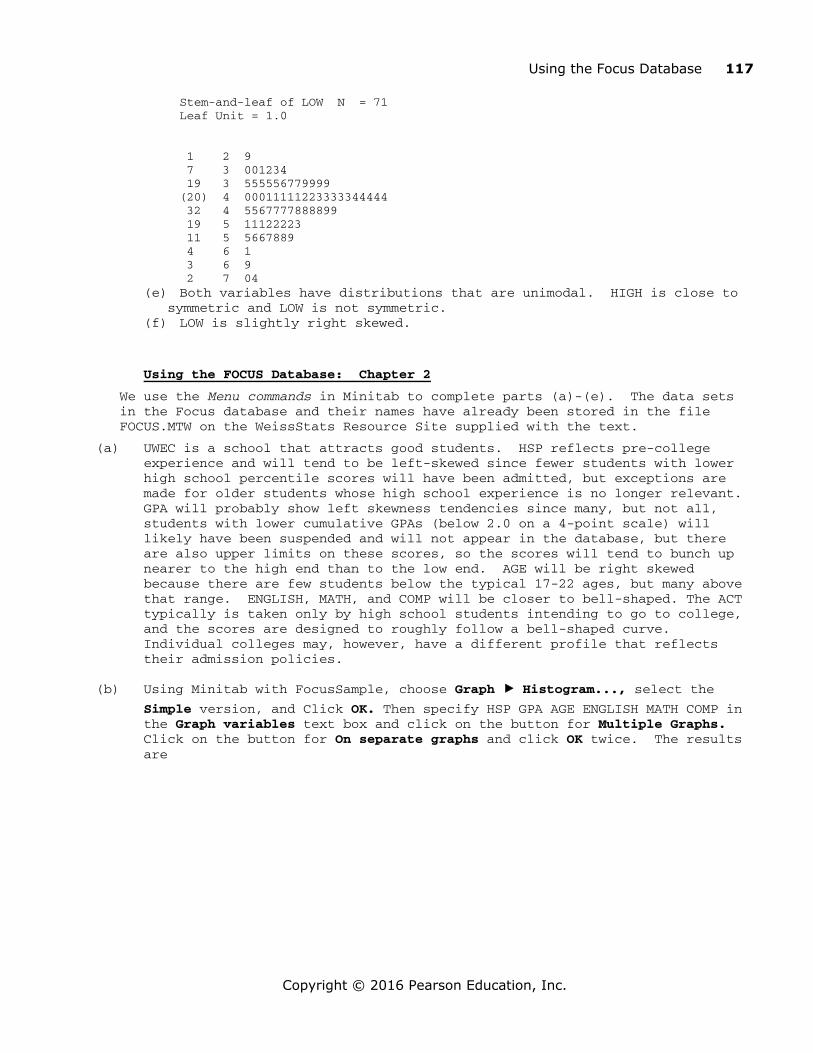
Using the Focus Database 117
Copyright © 2016 Pearson Education, Inc.
Stem-and-leaf of LOW N = 71 Leaf Unit = 1.0 1 2 9 7 3 001234 19 3 555556779999 (20) 4 00011111223333344444 32 4 5567777888899 19 5 11122223 11 5 5667889 4 6 1 3 6 9 2 7 04
(e) Both variables have distributions that are unimodal. HIGH is close to symmetric and LOW is not symmetric.
(f) LOW is slightly right skewed.
Using the FOCUS Database: Chapter 2
We use the Menu commands in Minitab to complete parts (a)-(e). The data sets in the Focus database and their names have already been stored in the file FOCUS.MTW on the WeissStats Resource Site supplied with the text.
(a) UWEC is a school that attracts good students. HSP reflects pre-college experience and will tend to be left-skewed since fewer students with lower high school percentile scores will have been admitted, but exceptions are made for older students whose high school experience is no longer relevant. GPA will probably show left skewness tendencies since many, but not all, students with lower cumulative GPAs (below 2.0 on a 4-point scale) will likely have been suspended and will not appear in the database, but there are also upper limits on these scores, so the scores will tend to bunch up nearer to the high end than to the low end. AGE will be right skewed because there are few students below the typical 17-22 ages, but many above that range. ENGLISH, MATH, and COMP will be closer to bell-shaped. The ACT typically is taken only by high school students intending to go to college, and the scores are designed to roughly follow a bell-shaped curve. Individual colleges may, however, have a different profile that reflects their admission policies.
(b) Using Minitab with FocusSample, choose Graph < Histogram..., select the Simple version, and Click OK. Then specify HSP GPA AGE ENGLISH MATH COMP in the Graph variables text box and click on the button for Multiple Graphs. Click on the button for On separate graphs and click OK twice. The results are

118 Chapter 2
Copyright © 2016 Pearson Education, Inc.
AGE
Freq
uenc
y
333027242118
50
40
30
20
10
0
Histogram of AGE
ENGLISH
Freq
uenc
y
36322824201612
40
30
20
10
0
Histogram of ENGLISH
MATH
Freq
uenc
y
33302724211815
25
20
15
10
5
0
Histogram of MATH
COMP
Freq
uenc
y
3230282624222018
30
25
20
15
10
5
0
Histogram of COMP
The graphs compare quite well with the educated guesses for all six variables.
(d) Using Minitab with Focus, choose Graph < Histogram..., select the Simple version, and Click OK. Then specify HSP GPA AGE ENGLISH MATH COMP in the Graph variables text box and click on the button for Multiple Graphs. Click on the button for On separate graphs and click OK twice. The results are
HSP
Freq
uenc
y
9075604530
25
20
15
10
5
0
Histogram of HSP
GPA
Freq
uenc
y
4.053.603.152.702.251.80
30
25
20
15
10
5
0
Histogram of GPA

Using the Focus Database 119
Copyright © 2016 Pearson Education, Inc.
AGE
Freq
uenc
y
403632282420
1800
1600
1400
1200
1000
800
600
400
200
0
Histogram of AGE
HSP
Freq
uenc
y
98847056422814
350
300
250
200
150
100
50
0
Histogram of HSP
ENGLISH
Freq
uenc
y
363228242016128
700
600
500
400
300
200
100
0
Histogram of ENGLISH
MATH
Freq
uenc
y
3633302724211815
700
600
500
400
300
200
100
0
Histogram of MATH
GPA
Freq
uenc
y
4.053.603.152.702.251.801.350.90
300
250
200
150
100
50
0
Histogram of GPA
We were correct on the first five variables: HSP and GPA are left skewed, AGE is right skewed, ENGLISH and MATH are fairly symmetric. COMP is close to symmetric, but is slightly right skewed. Comparing the graphs for the sample with those for the entire population, we see similarities between each pair of graphs, but the outline of the histogram for the entire population is much smoother than that of the histogram for the sample.
(d) Using Minitab and the FocusSample file, choose Graph < Piechart, click on the Chart raw data button, specify SEX CLASS RESIDENCY TYPE in the Graph variables text box and click on the Labels button. Now click on the tab for Slice Labels, check all four boxes and click OK, click on the button for
COMP
Freq
uenc
y
33302724211815
900
800
700
600
500
400
300
200
100
0
Histogram of COMP

120 Chapter 2
Copyright © 2016 Pearson Education, Inc.
Multiple Graphs and ensure that the button for On the same graph is checked, and click OK twice.
Once the graphs are displayed, we right clicked on the legend that was shown and selected Delete since we already had provided for each slice of the graphs to be labeled.
SEX CLASS
RESIDENCY TYPE
M82, 41.0%
F118, 59.0%
Sophomore59, 29.5%
Senior63, 31.5%
Junior53, 26.5%
Freshman25, 12.5%
Resident154, 77.0%
Nonresident46, 23.0%
Transfer22, 11.0%
Readmit2, 1.0%
New176, 88.0%
Pie Chart of SEX, CLASS, RESIDENCY, TYPE
From the graph of SEX, we see that about 59% of the students are females. From the graph of CLASS, we see that the student sample is about 12.5% Freshmen, 29.5% Sophomores, 26.5% Juniors, and 31.5% Seniors. From the graph of RESIDENCY, we see that about 77% of the students are Wisconsin residents and 23$ are nonresidents. From the graph of TYPE, we see that 88.0% of the students were admitted initially as new students, 11.0% were admitted initially as transfer students, and 1.0% are readmits, that is, students who were initially new or transfer students, left the university, and were later readmitted.
(e) Now repeat part (d) using the entire Focus file. The results are
SEX CLASS
RESIDENCY TYPE
M39.3%
F60.7%
Sophomore29.8%
Senior33.3%
Junior24.1%
Freshman12.8%
Other0.0%
Resident76.1%
Nonresident23.9%
Transfer11.1%
Readmit0.4%
New88.5%
Pie Chart of SEX, CLASS, RESIDENCY, TYPE
From the graph of SEX, we see that about 61% of the students are females. From the graph of CLASS, we see that the student population is about 13% Freshmen, 30% Sophomores, 24% Juniors, and 33% Seniors. From the graph of RESIDENCY, we see that about 76% of the students are Wisconsin residents and 24$ are nonresidents. From the graph of TYPE, we see that 85.5% of the

Case Study 121
Copyright © 2016 Pearson Education, Inc.
students were admitted initially as new students, 11.1% were admitted initially as transfer students, and 0.4% are readmits, that is, students who were initially new or transfer students, left the university, and were later readmitted. We would expect that the two sets of graphs would be approximately the same, but not identical since the sample contains only 200 students out of a population of 6738. This is, in fact, the case. The percentages in each sample graph are very close to the percentages in the corresponding population graph.
Case Study: World’s Richest People
(a) The first column variable is Rank and is quantitative discrete. The second column variable is Name and is qualitative. The third column variable is age and it is quantitative continuous. The fourth column variable is Citizenship and is qualitative. The fifth column variable is Wealth and is quantitative discrete since money involves discrete units, such as dollars and cents. Although, for all practical purposes, Wealth might be considered quantitative continuous data.
(b) The classes are the countries of citizenship and are presented in column 1. The frequency distribution of the champions is presented in column 2. Dividing each frequency by the total number of observations, which is 25, results in each class's relative frequency. The relative frequency distribution is presented in column 3.
Country Frequency Relative Frequency Canada 1 0.04
France 2 0.08
Germany 1 0.04
Hong Kong 2 0.08
India 1 0.04
Italy 1 0.04
Mexico 1 0.04
Spain 1 0.04
Sweden 1 0.04
United States 14 0.56
25 1.00
(c) We multiply each of the relative frequencies by 360 degrees to obtain the portion of the pie represented by each team. The result is
United States
CanadaFranceGermanyHong KongIndiaItalyMexicoSpainSweden
Category
United States56.0%
Sweden4.0%
Spain4.0%
Mexico4.0%
Italy4.0%
India4.0%
Hong Kong8.0%
Germany4.0%
France8.0%
Canada4.0%
Pie Chart of CITIZENSHIP
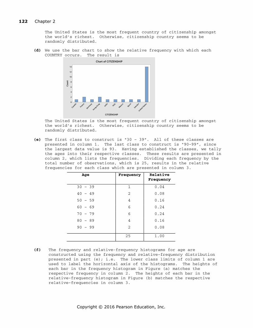
122 Chapter 2
Copyright © 2016 Pearson Education, Inc.
The United States is the most frequent country of citizenship amongst the world’s richest. Otherwise, citizenship country seems to be randomly distributed.
(d) We use the bar chart to show the relative frequency with which each
COUNTRY occurs. The result is
United
States
Sweden
Spain
MexicoIta
lyInd
ia
Hong Kong
Germany
France
Canad
a
1 4
1 2
1 0
8
6
4
2
0
CITIZENSHIP
Coun
t
Chart of CITIZENSHIP
The United States is the most frequent country of citizenship amongst the world’s richest. Otherwise, citizenship country seems to be randomly distributed.
(e) The first class to construct is "30 – 39”. All of these classes are
presented in column 1. The last class to construct is "90-99”, since the largest data value is 93. Having established the classes, we tally the ages into their respective classes. These results are presented in column 2, which lists the frequencies. Dividing each frequency by the total number of observations, which is 25, results in the relative frequencies for each class which are presented in column 3.
Age
Frequency RelativeFrequency
30 – 39 1 0.04
40 – 49 2 0.08
50 – 59 4 0.16
60 – 69 6 0.24
70 – 79 6 0.24
80 – 89 4 0.16
90 – 99 2 0.08
25 1.00
(f) The frequency and relative-frequency histograms for age are constructed using the frequency and relative-frequency distribution presented in part (e); i.e. The lower class limits of column 1 are used to label the horizontal axis of the histograms. The heights of each bar in the frequency histogram in Figure (a) matches the respective frequency in column 2. The heights of each bar in the relative-frequency histogram in Figure (b) matches the respective relative-frequencies in column 3.

Case Study 123
Copyright © 2016 Pearson Education, Inc.
Figure (a) Figure (b)
1 0090807060504030
6
5
4
3
2
1
0
AGE
Freq
uenc
y
Histogram of AGE
1 0090807060504030
25
20
1 5
1 0
5
0
AGE
Perc
ent
Histogram of AGE
(g) The shape of the distribution of age in part (e) is unimodal and is roughly symmetric.
(h) The stem-and-leaf diagram of age using one line per stem is
3| 9 4| 09 5| 5678 6| 345589 7| 133779 8| 2458 9| 03
The stem-and-leaf diagram of age using two lines per stem is
3| 9 4| 0 4| 9 5| 5| 5678 6| 34 6| 5589 7| 133 7| 779 8| 24 8| 58 9| 03
The stem-and-leaf diagram of age using one line per stem corresponds to the histogram in part (f).
(i) The dotplot for age is
88807264564840AGE
Dotplot of AGE
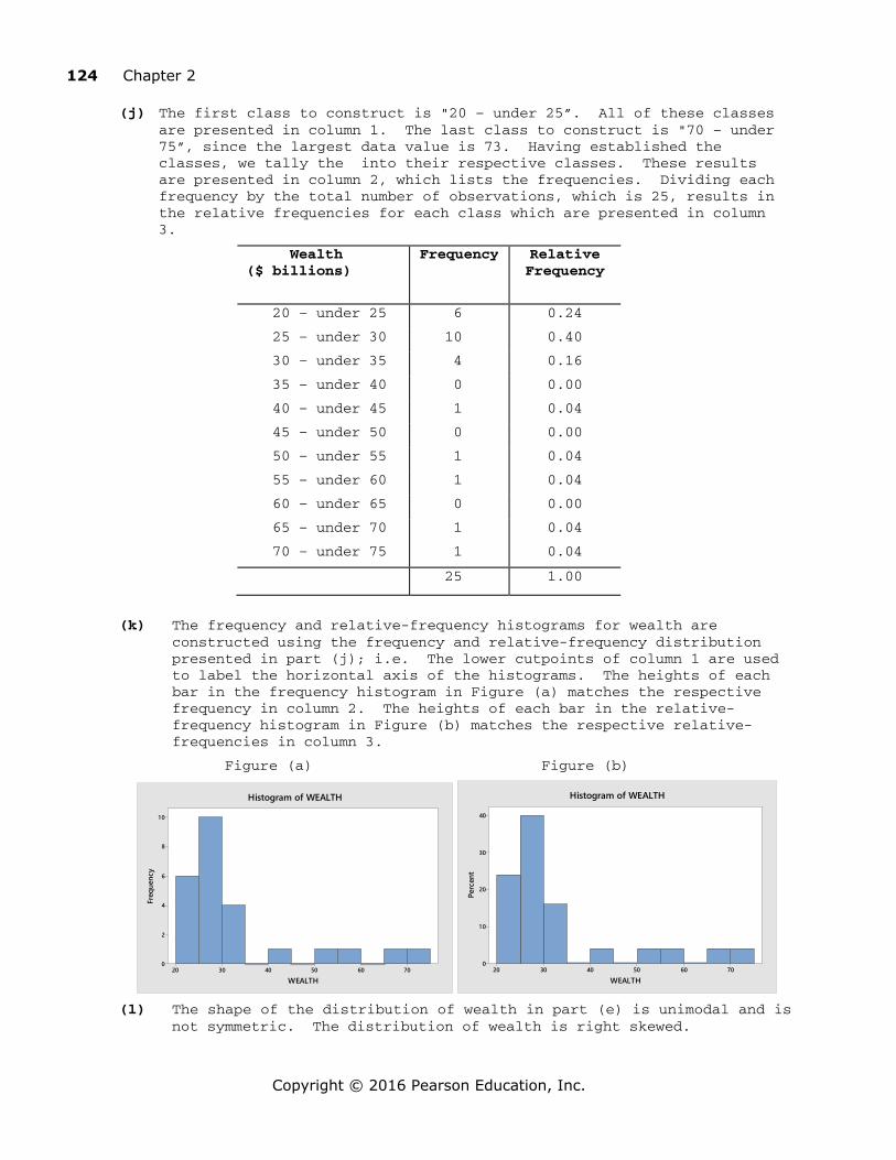
124 Chapter 2
Copyright © 2016 Pearson Education, Inc.
(j) The first class to construct is "20 – under 25”. All of these classes are presented in column 1. The last class to construct is "70 – under 75”, since the largest data value is 73. Having established the classes, we tally the into their respective classes. These results are presented in column 2, which lists the frequencies. Dividing each frequency by the total number of observations, which is 25, results in the relative frequencies for each class which are presented in column 3.
Wealth ($ billions)
Frequency RelativeFrequency
20 – under 25 6 0.24
25 – under 30 10 0.40
30 – under 35 4 0.16
35 – under 40 0 0.00
40 – under 45 1 0.04
45 – under 50 0 0.00
50 – under 55 1 0.04
55 – under 60 1 0.04
60 – under 65 0 0.00
65 – under 70 1 0.04
70 – under 75 1 0.04
25 1.00
(k) The frequency and relative-frequency histograms for wealth are constructed using the frequency and relative-frequency distribution presented in part (j); i.e. The lower cutpoints of column 1 are used to label the horizontal axis of the histograms. The heights of each bar in the frequency histogram in Figure (a) matches the respective frequency in column 2. The heights of each bar in the relative-frequency histogram in Figure (b) matches the respective relative-frequencies in column 3.
Figure (a) Figure (b)
706050403020
1 0
8
6
4
2
0
WEALTH
Freq
uenc
y
Histogram of WEALTH
706050403020
40
30
20
1 0
0
WEALTH
Perc
ent
Histogram of WEALTH
(l) The shape of the distribution of wealth in part (e) is unimodal and is
not symmetric. The distribution of wealth is right skewed.

Case Study 125
Copyright © 2016 Pearson Education, Inc.
(m) Truncating wealth to a whole number, the stem-and-leaf diagram using two lines per stem is
2| 000123 2| 5666667889 3| 0144 3| 4| 3 4| 5| 3 5| 7 6| 6| 7 7| 3
(n) Rounding wealth to a whole number, the dotplot is
7063564942352821Wealth ($ billions)
Dotplot of Wealth
