intrusion detection system using gated recurrent …

INTRUSION DETECTION SYSTEM USING GATED

RECURRENT NEURAL NETWORKS

A Project report submitted in partial fulfillment of the requirements for

the award of the degree of

BACHELOR OF TECHNOLOGY

IN

COMPUTER SCIENCE ENGINEERING

Submitted by

D. KIRAN MAHESH REDDY (316126510073)

B. DEEPIKA (316126510127)

G. ALEKHYA (316126510140)

CH. NAGA VENNELA (316126510134)

Under the guidance of

Mrs. G. PRANITHA

ASSISTANT PROFESSOR

DEPARTMENT OF COMPUTER SCIENCE AND ENGINEERING

ANIL NEERUKONDA INSTITUTE OF TECHNOLOGY AND SCIENCES

(UGC AUTONOMOUS)

(Permanently Affiliated to AU, Approved by AICTE and Accredited by NBA & NAAC with ‘A’ Grade)

Sangivalasa, bheemili mandal, visakhapatnam dist. (A.P)

2019-2020


ANIL NEERUKONDA INSTITUTE OF TECHNOLOGY AND SCIENCES

(UGC AUTONOMOUS)

(Affiliated to AU, Approved by AICTE and Accredited by NBA & NAAC with ‘A’

Grade)

Sangivalasa, Bheemili Mandal, Visakhapatnam dist.(A.P)

BONAFIDE CERTIFICATE

This is to certify that the project report entitled “INTRUSION DETECTION SYSTEM

USING GATED RECURRENT NEURAL NETWORKS” submitted by D. KIRAN

MAHESH REDDY (316126510073), B. DEEPIKA (316126510127), G. ALEKHYA

(316126510140), CH. NAGA VENNELA (316126510134) in partial fulfillment of the

requirements for the award of the degree of Bachelor of Technology in Computer Science

Engineering of Anil Neerukonda Institute of technology and sciences (A), Visakhapatnam

is a record of bonafide work carried out under my guidance and supervision.

Project Guide Head of the Department

Mrs. G. PRANITHA Dr. R. SIVARANJANI

Assistant Professor Professor

Department of CSE Department of CSE

ANITS ANITS

DECLARATION

We, D. KIRAN MAHESH REDDY, B. DEEPIKA, G. ALEKHYA, CH. NAGA

VENNELA, of final semester B.Tech, in the department of Computer Science and

Engineering from ANITS, Visakhapatnam, hereby declare that the project work entitled

“INTRUSION DETECTION SYSTEM USING GATED RECURRENT NEURAL

NETWORKS” is carried out by us and submitted in partial fulfillment of the requirements

for the award of Bachelor of Technology in Computer Science Engineering , under Anil

Neerukonda Institute of Technology & Sciences(A) during the academic year 2016-2020

and has not been submitted to any other university for the award of any kind of degree.

D. KIRAN MAHESH REDDY 316126510073

B. DEEPIKA 316126510127

G. ALEKHYA 316126510140

CH. NAGA VENNELA 316126510134

ACKNOWLEDGEMENT

We would like to express our deep gratitude to our project guide Mrs. G. Pranitha,

Assistant Professor, Department of Computer Science and Engineering, ANITS, for her

guidance with unsurpassed knowledge and immense encouragement. We are grateful to

Dr. R. Sivaranjani, Head of the Department, Computer Science and Engineering, for

providing us with the required facilities for the completion of the project work.

We are very much thankful to the Principal and Management, ANITS,

Sangivalasa, for their encouragement and cooperation to carry out this work.

We also thank our Project Coordinator Mrs. K. S. Deepthi for her support and

encouragement. We express our thanks to all teaching faculty of Department of Computer

Science and Engineering, whose suggestions during reviews helped us in accomplishment

of our project. We would like to thank Mrs. Udaya Lakshmi of the Department of

Computer Science and Engineering for providing us the lab resources in accomplishment

of our project.

We would like to thank our parents, friends, and classmates for their encouragement

throughout our project period. At last but not the least, we thank everyone for supporting

us directly or indirectly in completing this project successfully.

D. KIRAN MAHESH REDDY (316126510073)

B. DEEPIKA (316126510127)

G. ALEKHYA (316126510140)

CH. NAGA VENNELA (316126510134)

i

ABSTRACT

As use of the internet and related technologies which are spreading around the

world, the use of these networks now creates new threats for organizations. An Intrusion

detection system (IDS) plays a major role in preserving network security. So, we proposed

a deep learning-based Intrusion Detection System using recurrent neural networks with

gated recurrent units (GRU-IDS). The dataset used for evaluating the GRU-IDS is that the

NSL-KDD dataset. To reduce the dimensionality of the NSL-KDD dataset we used a

Random Forest classifier for feature selection. The experimental result suggests that the

performance of GRU-IDS is superior compared to traditional machine learning

classification methods.

Keywords- Intrusion detection, Recurrent Neural Network, Gated Recurrent Unit, GRU-

IDS, machine learning, deep learning.

ii

CONTENTS

TITLE Page No.

ABSTRACT i

LIST OF SYMBOLS v

LIST OF FIGURES vi

LIST OF TABLES viii

LIST OF ABBREVATIONS ix

CHAPTER 1. INTRODUCTION

1.1 Introduction 1

1.1.1 Intrusion Detection System 1

1.1.1.1 Types of Intrusion Detection System 2

1.1.1.2 Detection Methods of IDS 3

1.1.2 Machine Learning 3

1.1.2.1 Supervised Learning 4

1.1.2.2 Unsupervised Learning 6

1.1.2.3 Reinforcement Learning 7

1.1.3 Deep Learning 7

1.1.4 Neural Networks 8

1.1.5 Recurrent Neural Networks 9

1.1.5.1 Long Short-Term Memory 12

1.1.5.2 Gated Recurrent Unit 14

1.1.6 Random Forest Classifier 16

1.2 Motivation for the work 17

1.3 Problem Statement 17

1.4 Organization of the thesis 18

CHAPTER 2. LITERATURE SURVEY

2.1 Detailed Analysis on NSL-KDD Dataset Using Various Machine Learning

techniques

19

2.2 Performance Analysis of NSL-KDD dataset using ANN 19

iii

2.3 Ensemble Model for Classification of Attacks with Feature Selection 20

2.4 Feature Selection for Intrusion Detection using NSL-KDD 21

2.5 Deep Long Short-term memory-based classifier for wireless IDS 21

2.6 Deep Learning method with filter-based feature engineering for Wireless IDS 21

2.7 Study on NSL-KDD Dataset for IDS based on Classification Algorithms 22

2.8 Random Forest Modelling for Network Intrusion Detection System 22

2.9 Intrusion Detection System using Data Mining Technique 23

2.10 An Artificial Neural Network based IDS and Classification of Attacks 23

2.11 An effective IDS classifier using LSTM with gradient descent optimization 24

2.12 Existing System

24

CHAPTER 3. METHODOLOGY

3.1 Proposed System 25

3.1.1 System Architecture 25

3.1.2 Dataset Description 25

3.1.3 Flow of the System 31

3.1.4 Data Preprocessing 31

3.1.4.1 Conversion of Non-Numeric to numeric values 31

3.1.4.2 Normalization 32

3.1.5 Feature Selection 32

3.1.6 Working of Gated Recurrent Neural Network 34

3.2 Adam Optimizer 40

3.3 Hyper Parameter 41

3.4 Activation Functions 43

3.5 Evaluation Measures

47

CHAPTER 4. EXPERIMENTAL ANALYSIS AND RESULTS

4.1 System Configuration 49

4.1.1 Software Requirements 49

4.1.2 Hardware Requirements 55

iv

4.2 Sample Code Elaboration 56

4.2.1 Importing the required packages 56

4.2.2 Loading the NSL-KDD dataset 56

4.2.3 Conversion of symbolic features to numeric values 56

4.2.4 Normalization 57

4.2.5 Feature selection using Random Forest Classifier 58

4.2.6 Building the GRU-IDS model 59

4.3 Screenshots 63

4.4 Experimental Analysis and Results

69

CHAPTER 5. CONCLUSION AND FUTURE WORK

5.1 Conclusion 70

5.2 Future work 70

REFERENCES 71

APPENDICES 74

v

LIST OF SYMBOLS

∑ Summation

𝜎 Sigmoid Function

⊙ Hadamard Product

® Registered Trademark

vi

LIST OF FIGURES

Figure No. Topic Name Page No.

1.1 Machine Learning vs Traditional Programming 4

1.2 Neuron 9

1.3 Basic Neural Network 10

1.4 Unfolded Structure of Recurrent Neural Networks 11

1.5 LSTM Cell 13

1.6 GRU Cell 15

3.1 Proposed System 25

3.2 Flow of the System 31

3.3 Working of Random Forest Classifier 34

3.4 Recurrent Neural Network with Gated Recurrent Unit 34

3.5 Gated Recurrent Unit 35

3.6 Update Gate 36

3.7 Reset Gate 37

3.8 Current Memory Gate 38

3.9 Final Memory Gate 39

4.1 Performance of the GRU-IDS model on the training dataset for

epoch 30.

63

4.2 Performance of the GRU-IDS model on the test dataset for epoch

number 30.

63


epoch number 60.

64


number 60.

64


epoch number 120.

65


number 120.

65

vii


epoch number 180.

66


number 180.

66


epoch number 200.

67


number 200.

67


epoch number 300.

68


number 300.

68

viii

LIST OF TABLES

Table No. Topic Name Page No.

3.1 Features of NSL-KDD Dataset 26

3.2 Confusion Matrix 46

4.1 Performance measures of the existing systems 69

4.2 Performance measures of the proposed system 69

ix

LIST OF ABBREVATIONS

IDS Intrusion Detection System

IDPS Intrusion Detection and Prevention System

NIDS Network Intrusion Detection System

HIDS Host Intrusion Detection System

SVM Support Vector Machine

ANN Artificial Neural Networks

KNN k-nearest neighbor

ML Machine Learning

RL Reinforcement Learning

AI Artificial Intelligence

DBN Deep Belief Network

RNN Recurrent Neural Network

LSTM Long Short-Term Memory

GRU Gated Recurrent Unit

RF Random Forest

KDD Knowledge Discovery in Databases

DLSTM Deep Long Short-Term Memory

FFDNN Feed Forward Deep Neural Network

SGD Stochastic Gradient Descent

RMSprop Root Mean Square Propagation

AC Accuracy

TP True Positive

FP False Positive

TN True Negative

FN False Negative

TPR True Positive Rate

DR Detection Rate

PR Precision

FPR False Positive Rate

1

1. INTRODUCTION

1.1. INTRODUCTION

We are now living in a borderless world where there is nothing to break-in i.e, either

the building or computer system. Even though the technology is being elevated, it also has

given rise to new vulnerabilities and threats to the organizations. Intrusion detection system

(IDS) is a type of security management system for computers and networks. An intrusion

detection system (IDS) inspects all outbound and inbound network actions and finds out

the doubtful patterns that may point to network or system intrusion or attack from someone

trying to crack into or conciliate a system. The traditional machine learning technologies

like SVMs, ANNs, Random Forest, Naive Bayes, KNN and J48 have shown good results

in intrusion detection but also have some limitations in performance accuracy. To improve

the performance in intrusion detection we introduced a deep learning-based recurrent

neural network with gated recurrent units. So, we have decided to build up an IDS model

which can detect any abnormal behavior in the network.

1.1. 1. INTRUSION DETECTION SYSTEM

An Intrusion Detection System (IDS) is a system that monitors network traffic for

suspicious activity and issues alerts when such activity is discovered. It is a software

application that scans a network or a system for harmful activity or policy breaching.

Intrusion refers to an unauthorized access to a system or a service by compromising the

system to enter an insecure state. An Intrusion can be featured in terms of Confidentiality,

Integrity, Availability. Confidentiality indicates protecting information from an

unauthorized user. Integrity ensures that the data is accurate and safe guarded even after an

intruder’s modification. Availability brings up the ability to the user to access information

in correct format. The user who does intrusion is called an intruder, who leaves some traces

which are being detected by an Intrusion detection system. Although intrusion detection

systems monitor networks for potentially malicious activity, they are also disposed to false

alarms. Hence, organizations need to fine-tune their IDS products when they first install

them. It means properly setting up the intrusion detection systems to recognize what normal

traffic on the network looks like as compared to malicious activity. Intrusion detection

2

systems offer organizations several benefits, starting with the ability to identify security

incidents. An IDS can be used to help analyze the quantity and types of attacks;

organizations can use this information to change their security systems or implement more

effective controls. An intrusion detection system can also help companies identify bugs or

problems with their network device configurations. These metrics can then be used to

assess future risks. Historically, intrusion detection systems were categorized as passive or

active. A passive IDS that detected malicious activity would generate alert or log entries

but would not take action; an active IDS, sometimes called an intrusion detection and

prevention system (IDPS), would generate alerts and log entries but could also be

configured to take actions, like blocking IP addresses or shutting down access to restricted

resources.

1.1.1.1. TYPES OF INTRUSION DETECTION SYSTEM

• Network Intrusion Detection System (NIDS)

Network intrusion detection systems (NIDS) are set up at a planned point

within the network to examine traffic from all devices on the network. It performs

an observation of passing traffic on the entire subnet and matches the traffic that is

passed on the subnets to the collection of known attacks. Once an attack is identified

or abnormal behavior is observed, the alert can be sent to the administrator. An

example of an NIDS is installing it on the subnet where firewalls are located in

order to see if someone is trying crack the firewall.

• Host Intrusion Detection System (HIDS):

Host intrusion detection systems (HIDS) run on independent hosts or devices

on the network. A HIDS monitors the incoming and outgoing packets from the

device only and will alert the administrator if suspicious or malicious activity is

detected. A HIDS has an advantage over a NIDS in that it may be able to detect

anomalous network packets that originate from inside the organization or malicious

traffic that a NIDS has failed to detect. A HIDS may also be able to identify

malicious traffic that originates from the host itself, such as when the host has been

infected with malware and is attempting to spread to other systems.

3

1.1.1.2. DETECTION METHODS OF IDS:

The two primary methods of detection are signature-based and anomaly-based. Any type

of IDS can detect attacks based on signatures, anomalies, or both.

• Signature-based IDS detects the attacks based on the specific patterns such as

number of bytes or number of 1’s or number of 0’s in the network traffic. It also

detects based on the already known malicious instruction sequence that is used by

the malware. The detected patterns in the IDS are known as signatures. It can easily

detect the attacks whose pattern (signature) already exists in system but it is quite

difficult to detect the new malware attacks as their pattern (signature) is not known.

• Anomaly-based IDS was introduced to detect the unknown malware attacks as

new malware are developed rapidly. In anomaly-based IDS there is use of machine

learning to create a trustful activity model and anything coming is compared with

that model and it is declared suspicious if it is not found in model. Machine learning

based method has a better generalized property in comparison to signature-based

IDS as these models can be trained according to the applications and hardware

configurations.

1.1.2. MACHINE LEARNING:

Machine Learning is undeniably one of the most influential and powerful

technologies in today’s world. More importantly, we are far from seeing its full potential.

Machine Learning is a concept which allows the machine to learn from examples and

experiences. It is a subset of Artificial Intelligence that comprises algorithms programmed

to gather information without explicit instructions at each step. Machine learning is a tool

for turning information into knowledge and is transforming the world by enabling machines

to do all sorts of ‘intelligent’ tasks such as understanding images, human speech, predicting

preferences and many others. With tremendous amount of data, interconnectedness and

huge processing power in small devices, machines are doing things which were not

anticipated until recently. In the past 50 years, there has been an explosion of data. This

mass of data is useless unless we analyze it and find the patterns hidden within. Machine

learning techniques are used to automatically find the valuable underlying patterns within

complex data that we would otherwise struggle to discover. The hidden patterns and

4

knowledge about a problem can be used to predict future events and perform all kinds of

complex decision making. Machine Learning algorithm is trained using a training data set

to create a model. When new input data is introduced to the ML algorithm, it makes a

prediction on the basis of model. The prediction is evaluated for accuracy and if the

accuracy is acceptable, the Machine Learning algorithm is deployed, If the accuracy is not

acceptable, the Machine Learning algorithm is trained again and again with an augmented

training data set.

Figure 1.1 Machine Learning vs Traditional Programming

Types of Machine Learning Algorithms

1. Supervised learning – Train Me!

2. Unsupervised Learning – I am self-sufficient in learning

3. Reinforcement Learning – My life My rules!

1.1.2.1 SUPERVISED LEARNING

Supervised learning is the most popular paradigm for machine learning. It is the

easiest to understand and the simplest to implement. It is the machine learning task of

learning a function that maps an input to an output based on example input-output pairs. It

infers a function from labelled training data consisting of a set of training examples. In

supervised learning, each example is a pair consisting of an input object (typically a vector)

and a desired output value (also called the supervisory signal). A supervised learning

algorithm analyses the training data and produces an inferred function, which can be used

for mapping new examples. Supervised Learning is very similar to teaching a child with the

given data and that data is in the form of examples with labels, we can feed a learning

algorithm with these example-label pairs one by one, allowing the algorithm to predict the

5

right answer or not. Over time, the algorithm will learn to approximate the exact nature of

the relationship between examples and their labels. When fully trained, the supervised

learning algorithm will be able to observe a new, never-before-seen example and predict a

good label for it.

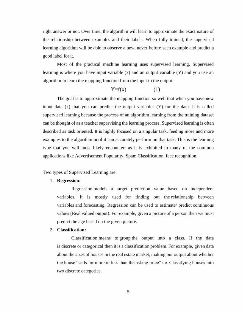
Most of the practical machine learning uses supervised learning. Supervised

learning is where you have input variable (x) and an output variable (Y) and you use an

algorithm to learn the mapping function from the input to the output.

Y=f(x) (1)

The goal is to approximate the mapping function so well that when you have new

input data (x) that you can predict the output variables (Y) for the data. It is called

supervised learning because the process of an algorithm learning from the training dataset

can be thought of as a teacher supervising the learning process. Supervised learning is often

described as task oriented. It is highly focused on a singular task, feeding more and more

examples to the algorithm until it can accurately perform on that task. This is the learning

type that you will most likely encounter, as it is exhibited in many of the common

applications like Advertisement Popularity, Spam Classification, face recognition.

Two types of Supervised Learning are:

1. Regression:

Regression models a target prediction value based on independent

variables. It is mostly used for finding out the relationship between

variables and forecasting. Regression can be used to estimate/ predict continuous

values (Real valued output). For example, given a picture of a person then we must

predict the age based on the given picture.

2. Classification:

Classification means to group the output into a class. If the data

is discrete or categorical then it is a classification problem. For example, given data

about the sizes of houses in the real estate market, making our output about whether

the house “sells for more or less than the asking price” i.e. Classifying houses into

two discrete categories.

6

1.1.2.2 UNSUPERVISED LEARNING

Unsupervised Learning is a machine learning technique, where you do not need to

supervise the model. Instead, you need to allow the model to work on its own to discover

information. It mainly deals with the unlabeled data and looks for previously undetected

patterns in a data set with no pre-existing labels and with a minimum of human supervision.

In contrast to supervised learning that usually makes use of human-labeled data,

unsupervised learning, also known as self-organization, allows for modelling of probability

densities over inputs.

Unsupervised machine learning algorithms infer patterns from a dataset without

reference to known or labeled outcomes. It is the training of machine using information

that is neither classified nor labeled and allowing the algorithm to act on that information

without guidance. Here the task of machine is to group unsorted information according to

similarities, patterns, and differences without any prior training of data. Unlike supervised

learning, no teacher is present that means no training will be given to the machine.

Therefore, machine is restricted to find the hidden structure in unlabeled data by our-self.

For example, if we provide some pictures of dogs and cats to the machine to categorized,

then initially the machine has no idea about the features of dogs and cats, so it categorizes

them according to their similarities, patterns and differences. The Unsupervised Learning

algorithms allows you to perform more complex processing tasks compared to supervised

learning. Although, unsupervised learning can be more unpredictable compared with other

natural learning methods.

Unsupervised learning problems are classified into two categories of algorithms:

• Clustering: A clustering problem is where you want to discover the inherent

groupings in the data, such as grouping customers by purchasing behavior.

• Association: An association rule learning problem is where you want to discover

rules that describe large portions of your data, such as people that buy X also tend

to buy Y.

7

1.1.2.3 REINFORCEMENT LEARNING

Reinforcement Learning (RL) is a type of machine learning technique that enables

an agent to learn in an interactive environment by trial and error using feedback from its

own actions and experiences. Machine mainly learns from past experiences and tries to

perform best possible solution to a certain problem. It is the training of machine learning

models to make a sequence of decisions. Though both supervised and reinforcement

learning use mapping between input and output, unlike supervised learning where the

feedback provided to the agent is correct set of actions for performing a task, reinforcement

learning uses rewards and punishments as signals for positive and negative behavior.

Reinforcement learning is currently the most effective way to hint machine’s creativity.

1.1.3. DEEP LEARNING

Deep learning is a branch of machine learning which is completely based

on artificial neural networks, as neural network is going to mimic the human brain so deep

learning is also a kind of mimic of human brain. In deep learning, we don’t need to

explicitly program everything. The concept of deep learning is not new. It has been around

for a couple of years now. It is on hype nowadays because earlier we did not have that

much processing power and a lot of data. As in the last 20 years, the processing power

increases exponentially, deep learning and machine learning came in the picture.

Deep learning is an artificial intelligence function that imitates the workings of the

human brain in processing data and creating patterns for use in decision making. Deep

learning is a subset of machine learning in artificial intelligence (AI) that has networks

capable of learning unsupervised from data that is unstructured or unlabelled. It has a

greater number of hidden layers and known as deep neural learning or deep neural network.

Deep learning has evolved together with the digital era, which has brought about an

explosion of data in all forms and from every region of the world. This data, known simply

as big data, is drawn from sources like social media, internet search engines, e-

commerce platforms, and online cinemas, among others. This enormous amount of data is

readily accessible and can be shared through fintech applications like cloud computing.

However, the data, which normally is unstructured, is so vast that it could take decades for

humans to comprehend it and extract relevant information. Companies realize the

https://www.geeksforgeeks.org/introduction-machine-learning/

https://www.geeksforgeeks.org/tag/neural-network/

8

incredible potential that can result from unravelling this wealth of information and are

increasingly adapting to AI systems for automated support. Deep learning learns from vast

amounts of unstructured data that would normally take humans decades to understand and

process. Deep learning utilizes a hierarchical level of artificial neural networks to carry out

the process of machine learning. The artificial neural networks are built like the human

brain, with neuron nodes connected like a web. While traditional programs build analysis

with data in a linear way, the hierarchical function of deep learning systems enables

machines to process data with a nonlinear approach.

Architectures:

1. Deep Neural Network – It is a neural network with a certain level of complexity

(having multiple hidden layers in between input and output layers). They are

capable of modelling and processing non-linear relationships.

2. Deep Belief Network (DBN) – It is a class of Deep Neural Network. It is multi-

layer belief networks.

Steps for performing DBN:

a. Learn a layer of features from visible units using

Contrastive Divergence algorithm.

b. Treat activations of previously trained features as visible

units and then learn features of features.

c. Finally, the whole DBN is trained when the learning for the

final hidden layer is achieved.

3. Recurrent (perform same task for every element of a sequence) Neural Network –

Allows for parallel and sequential computation. Like the human brain (large

feedback network of connected neurons). They can remember important things

about the input they received and hence enables them to be more precise.

1.1.4. NEURAL NETWORKS

Neural Network (or Artificial Neural Network) can learn by examples. ANN is an

information processing model inspired by the biological neuron system. ANN biologically

inspired simulations that are performed on the computer to do a certain specific set of tasks

like clustering, classification, pattern recognition etc. It is composed of many highly

9

interconnected processing elements known as the neuron to solve problems. It follows the

non-linear path and process information in parallel throughout the nodes. A neural network

is a complex adaptive system. Adaptive means it can change its internal structure by

adjusting weights of inputs.

Artificial Neural Networks can be best viewed as weighted directed graphs, where

the nodes are formed by the artificial neurons and the connection between the neuron

outputs and neuron inputs can be represented by the directed edges with weights. The ANN

receives the input signal from the external world in the form of a pattern and image in the

form of a vector. These inputs are then mathematically designated by the notations x(n) for

every n number of inputs. Each of the input is then multiplied by its corresponding weights

(these weights are the details used by the artificial neural networks to solve a certain

problem). These weights typically represent the strength of the interconnection amongst

neurons inside the artificial neural network. All the weighted inputs are summed up inside

the computing unit (yet another artificial neuron).

If the weighted sum equates to zero, a bias is added to make the output non-zero or

else to scale up to the system’s response. Bias has the weight and the input to it is always

equal to 1. Here the sum of weighted inputs can be in the range of 0 to positive infinity. To

keep the response in the limits of the desired values, a certain threshold value is

benchmarked. And then the sum of weighted inputs is passed through the activation

function. The activation function is the set of transfer functions used to get the desired

output of it. There are various flavors of the activation function, but mainly either linear or

non-linear set of functions. Some of the most used set of activation functions are the Binary,

Sigmoid (linear) and Tan hyperbolic sigmoidal (non-linear) activation functions.

Figure 1.2 Neuron

10

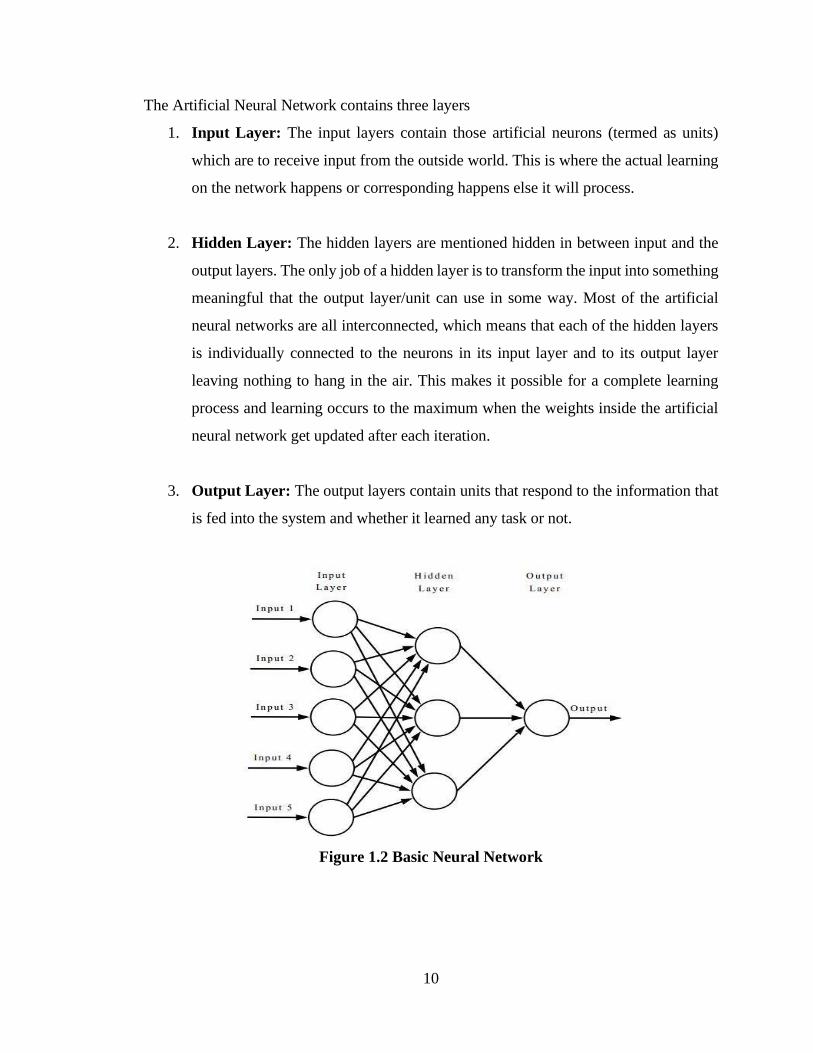
The Artificial Neural Network contains three layers

1. Input Layer: The input layers contain those artificial neurons (termed as units)

which are to receive input from the outside world. This is where the actual learning

on the network happens or corresponding happens else it will process.

2. Hidden Layer: The hidden layers are mentioned hidden in between input and the

output layers. The only job of a hidden layer is to transform the input into something

meaningful that the output layer/unit can use in some way. Most of the artificial

neural networks are all interconnected, which means that each of the hidden layers

is individually connected to the neurons in its input layer and to its output layer

leaving nothing to hang in the air. This makes it possible for a complete learning

process and learning occurs to the maximum when the weights inside the artificial

neural network get updated after each iteration.

3. Output Layer: The output layers contain units that respond to the information that

is fed into the system and whether it learned any task or not.

Figure 1.2 Basic Neural Network

11

1.1.5. RECURRENT NEURAL NETWORKS(RNN)

Recurrent Neural Network (RNN) are a type of Neural Network where the output

from previous step are fed as input to the current step. In traditional neural networks, all

the inputs and outputs are independent of each other, but in cases like when it is required

to predict the next word of a sentence, the previous words are required and hence there is

a need to remember the previous words. Thus, RNN came into existence, which solved this

issue with the help of a Hidden Layer. The main and most important feature of RNN

is Hidden state, which remembers some information about a sequence. A Recurrent Neural

Network (RNN) is a class of artificial neural networks where connections form a directed

graph along a temporal sequence. RNNs are used in deep learning and in the development

of models that simulate the activity of neurons in the human brain. An RNN consists of the

input layer, hidden layer, and an output layer. The main important feature of RNN is the

hidden state which acts like an interface between the input state and output state. RNNs are

different from the traditional feedforward neural networks because it consists of a

directional loop that acts as a memory for storing the previous state's information. Hidden

layers can be more than one depending upon the complexity of the project.

Figure 1.3 Unfolded Structure of Recurrent Neural Networks

The Recurrent Neural Network consists of two weight matrices. The weight matrix

W between the input layer and the hidden layer. The weight matrix U between the hidden

layer at time step t and the other hidden layer at time step t-1.

https://www.geeksforgeeks.org/tag/neural-network/

12

Formula for calculating current state:

ht = f (ht–1, xt) (2)

Where,

ht -> current state

ht-1 -> previous state

xt -> input state

Formula for current hidden state:

ht = tanh (Whh h t-1 + Wxh xt) (3)

Where,

Whh -> weight at recurrent neuron.

Wxh -> weight at input neuron.

Formula for calculating output:

yt = Why ht (4)

Where,

yt -> output

Why -> weight at output layer.

Advantages of Recurrent Neural Network:

1. An RNN remembers each information through time. It is useful in time series

prediction only because of the feature to remember previous inputs as well. This is

called Long Short-Term Memory.

2. Recurrent neural network is even used with convolutional layers to extend the

effective pixel neighbourhood.

Disadvantages of Recurrent Neural Network:

1. Gradient vanishing and exploding problems.

2. Training an RNN is a very difficult task.

3. It cannot process very long sequences if using tanh or relu as an activation function.

1.1.5.1 LONG SHORT-TERM MEMORY(LSTM)

To solve the problem of Vanishing and Exploding Gradients in a deep Recurrent

Neural Network, many variations were developed. One of the most famous of them is

13

the Long Short-Term Memory Network (LSTM). In concept, an LSTM recurrent unit tries

to “remember” all the past knowledge that the network is seen so far and to “forget”

irrelevant data. This is done by introducing different activation function layers called

“gates” for different purposes. Each LSTM recurrent unit also maintains a vector called

the Internal Cell State which conceptually describes the information that was chosen to be

retained by the previous LSTM recurrent unit. A Long Short-Term Memory Network

consists of four different gates for different purposes as described below: -

1. Forget Gate(f): It determines to what extent to forget the previous data.

2. Input Gate(i): It determines the extent of information to be written onto the

Internal Cell State.

3. Input Modulation Gate(g): It is often considered as a sub-part of the input gate

and many literatures on LSTM’s do not even mention it and assume it inside the

Input gate. It is used to modulate the information that the Input gate will write onto

the Internal State Cell by adding non-linearity to the information and making the

information Zero-mean. This is done to reduce the learning time as Zero-mean

input has faster convergence. Although this gate’s actions are less important than

the others and is often treated as a finesse-providing concept, it is good practice to

include this gate into the structure of the LSTM unit.

4. Output Gate(o): It determines what output (next Hidden State) to generate from

the current Internal Cell State.

Figure 1.5 LSTM CELL

14

Working of an LSTM recurrent unit:

1. Take input the current input, the previous hidden state and the previous internal cell

state.

2. Calculate the values of the four different gates by following the below steps: -

3. For each gate, calculate the parameterized vectors for the current input and the

previous hidden state by element-wise multiplication with the concerned vector

with the respective weights for each gate.

4. Apply the respective activation function for each gate elementwise on the

parameterized vectors. Below given is the list of the gates with the activation

function to be applied for the gate.

a. Input Gate: Sigmoid Function

b. Forget Gate: Sigmoid Function

c. Output Gate: Sigmoid Function

d. Input Modulation Gate: Hyperbolic Tangent Function

5. Calculate the current internal cell state by first calculating the element-wise

multiplication vector of the input gate and the input modulation gate, then calculate

the element-wise multiplication vector of the forget gate and the previous internal

cell state and then adding the two vectors.

ct = i ⊙ g + f ⊙ ct-1 (5)

6. Calculate the current hidden state by first taking the element-wise hyperbolic

tangent of the current internal cell state vector and then performing element wise

multiplication with the output gate.

ht = o ⊙ tanh(ct) (6)

1.1.5.2 GATED RECURRENT UNIT(GRU):

To solve the Vanishing-Exploding gradients problem often encountered during the

operation of a basic Recurrent Neural Network, many variations were developed. One of

the most famous variations is the Long Short-Term Memory Network (LSTM). One of the

lesser known but equally effective variations is the Gated Recurrent Unit Network (GRU).

15

Unlike LSTM, it consists of only three gates and does not maintain an Internal Cell State.

The information which is stored in the Internal Cell State in an LSTM recurrent unit is

incorporated into the hidden state of the Gated Recurrent Unit. This collective information

is passed onto the next Gated Recurrent Unit.

The different gates of a GRU are as described below: -

1. Update Gate(z): It determines how much of the past knowledge needs to be passed

along into the future. It is analogous to the Output Gate in an LSTM recurrent unit.

2. Reset Gate(r): It determines how much of the past knowledge to forget. It is

analogous to the combination of the Input Gate and the Forget Gate in an LSTM

recurrent unit.

3. Current Memory Gate(𝒉t): It is often overlooked during a typical discussion on

Gated Recurrent Unit Network. It is incorporated into the Reset Gate just like the

Input Modulation Gate is a sub-part of the Input Gate and is used to introduce some

non-linearity into the input and to also make the input Zero-mean. Another reason

to make it a sub-part of the Reset gate is to reduce the effect that previous

information has on the current information that is being passed into the future.

Figure 1.6 GRU CELL

Where,

xₜ = input at time step t.

hₜ = hidden layer input at time step t.

zₜ = update gate output at time step t.

rₜ = reset gate output at time step t.

16

1.1.6 RANDOM FOREST CLASSIFIER

Random forests are one the most popular machine learning algorithms. They are so

successful because they provide in general a good predictive performance, low overfitting,

and easy interpretability. This interpretability is given by the fact that it is straightforward

to derive the importance of each variable on the tree decision. In other words, it is easy to

compute how much each variable is contributing to the decision. Feature selection using

Random forest comes under the category of Embedded methods. Embedded methods

combine the qualities of filter and wrapper methods. They are implemented by algorithms

that have their own built-in feature selection methods. Random forest has low classification

error compared to other traditional classification algorithms.

Some of the benefits of RF are:

1. Ability to handle numerous input variables without a necessity for variable deletion.

2. Can run on huge data bases efficiently.

3. Provides estimates of important variables for the classification.

4. Random forest overcomes the problem over fitting.

5. Robust to noise and outliers when compared to single classifiers.

6. Lightweight when compared to other boosting methods.

We have made use of the ability of the random classifier method to rank the importance

of the features set to the target variables. We have selected those variables based on the

maximum importance levels. Those features with low values of the importance will add

less information to the learning model and are ignored based on the threshold values of the

importance.

17

1.2 MOTIVATION FOR THE WORK

With the increasingly deep integration of the internet and society, the internet is

changing the way in which people live, study and work, but the various security threats

that we face are becoming more and more serious. So, there is a need for Intrusion

Detection System. To identify these various network attacks, especially unforeseen attacks

is an unavoidable key technical issue. So, we thought of developing an intrusion-detection

system which could be a significant research achievement in the information security field,

can identify an invasion, which could be an ongoing invasion or an intrusion that had

already occurred.

In this project we have chosen the Gated Recurrent Unit (GRU) for implementation.

The basic workflow of a Gated Recurrent Unit Network is like that of a basic RNN which

is illustrated earlier, the main difference between the two is their internal working.

Recurrent Neural Networks suffer from short-term memory. So, LSTM’s and GRU’s were

created as the solution to short-term memory. They have internal mechanisms called gates

that can regulate the flow of information. The gates can learn which data in a sequence is

important to keep or throw away. By doing that, it can pass relevant information down the

long chain of sequences to make predictions. We have decided to work with GRU because

LSTM’s control the exposure of memory content (cell state) while GRU’s expose the entire

cell state to other units in the network. The LSTM unit has separate input and forget gates,

while the GRU performs both operations together via its reset gate. GRU use less training

parameters and use less memory, execute faster and train faster than LSTM.

1.3 PROBLEM STATEMENT

Most of the organizations suffer from attacks which are both from outside and

inside the network. The attacks from outside the network can be handled using firewalls.

But the attacks from inside the network cannot be detected easily. So, there is a need for

Intrusion Detection System which should be accurate enough to detect the unforeseen

attacks in a network. This project proposes a methodology that uses a deep learning

approach using gated recurrent neural networks which is better than traditional machine

learning classification methods to classify a record as an attack or a normal record.

18

1.4 ORGANIZATION OF THE THESIS

Chapter 1 discusses about the introduction to the project and it tells about the tools that is

used for developing the project.

Remaining chapters of the report describes as follows:

Chapter 2 specifies literature survey which includes different existing methods for

constructing the Intrusion Detection System.

Chapter 3 describes about the methodology which includes the system architecture, pre-

processing steps and implementation of our proposed system.

Chapter 4 describes about the software and hardware requirements for the execution of

our proposed system (GRU-IDS), sample code of our project and the experimental results

of our work along with the output screen shots.

Chapter 5 specifies the conclusion and future work.

19

2. LITERATURE SURVEY

2.1. A Detailed Analysis on NSL-KDD Dataset Using Various Machine

Learning Techniques for Intrusion Detection by S. Revathi, A. Malathi.

In [1], they had conducted a detailed study on KDD cup 99 as well as NSL-KDD

dataset which is an updated version of KDD cup 99 so that they can provide a good analysis

on various machine learning techniques for intrusion detection they had classified the

attacks into 4 major attacks i.e, Denial of Service (DoS),Probe, Remote to Local (R2L),

User to Root (U2R), which are present in the dataset, both in testing and training datasets.

They also conducted test accuracy using data mining techniques i.e, Random forest, J48,

SVM, CART and Naive Bayes. And the result has shown that Random Forest has high test

accuracy compared to all other algorithms. So, we are taking this into consideration and

applying this random forest classifier for feature selection.

2.2. Performance Analysis of NSL-KDD dataset using ANN by

Bhupendra Ingre, Anamika Yadav.

In [2], they had conducted performance analysis of NSL-KDD dataset using ANN

which included description of dataset’s i.e,

1. DARPA datasets (1998, 1999 and 2000).

2. The KDD 99 intrusion data is derived from DARPA 98 dataset. Dataset contain 41

features and one more attribute for class.

3. NSL-KDD dataset is offline network data based on KDD 99 dataset. It is an updated

version of KDD 99 dataset which removed all the redundant records.

The methodology which they had proposed applied on NSL-KDD dataset which

having 41 attribute and one class attribute. The training set of NSL-KDD does not include

redundant record and hence reduce the complexity level. There are various advantages of

NSL-KDD data set over the original KDD dataset which were discussed. The training is

performed on KDD Train data which contain 22 attack types and testing is performed on

KDD Test data which contains additional 17 attack type. These attacks can be categories

in four different types with some common properties. The four categories of attacks are:

Denial of Service (DoS), Probe, Remote to Local (R2L), User to Root (U2R). They

20

performed this experiment on MATLAB. Neural network with different hidden layer and

algorithm is used for training 18718 selected patterns and testing 22544 patterns of NSL-

KDD dataset. Training and testing performed on 41 and 29 selected features NSL dataset

with various values of neural network architecture. The training and testing with 41

attributes require more time as compare to 29 selected attributes. The result obtained for

both binary class as well as five class classification (type of attack). Results are analyzed

based on various performance measures and better accuracy was found. The detection rate

obtained is 81.2% and 79.9% for intrusion detection and attack type classification task

respectively for NSLKDD dataset. The performance of the proposed scheme has been

compared with existing scheme and higher detection rate is achieved in both binary class

as well as five class classification problems.

2.3. An Ensemble Model for Classification of Attacks with Feature

Selection based on KDD99 and NSL-KDD Dataset by AK Shrivas, AK

Dewangan.

In [3], they have ensembled two techniques as Artificial Neural Network (ANN)

and Bayesian Net. This ensemble model gives higher accuracy compared two each

individual model like ANN and Bayesian Net. Feature selection is also one of the most

important roles to reduce the irrelevant features and improve classification accuracy. Gain

Ratio (GR) feature selection applied on ensemble of ANN and Bayesian Net techniques

which gives higher accuracy with a smaller number of features. They also have conducted

experiment on Different attacks and normal category along with sample size of both

KDDCUP99 and NSL-KDD data sets.

Simulated results have shown that accuracy for proposed ensemble of ANN and

Bayesian Net is the best as compare to its individuals and other ensemble models. Accuracy

of proposed model is consistent (99.41%) in case of KDD99 data set with all partitions of

data set like 70-30%, 80-20% and 90-10% as training-testing, but accuracy of proposed

model is highest 97.76% in case of NSL-KDD data set with 80-20% training-testing

partitions.

21

2.4. Feature Selection for Intrusion Detection using NSL-KDD by Hee-su

Chae, Byung-oh Jo, Sang-Hyun Choi, Twae-kyung Park.

In [4], they had discussed a detailed description about NSL-KDD dataset and the

types of attacks. They had proposed a new feature selection method using feature average

of total and each class. And they applied one of the efficient classifier decision tree

algorithms for evaluating feature reduction methods and compared proposed methods and

other method. They had calculated the accuracy for the accumulation of the number of

features using the AR ranker and the accuracy of AR, CFS, IG, and GR for the

accumulation of the number of features and Full data. The result had shown the inverse

correlation between accuracy and AR up to 22 features. It was clear that the highest

accuracy is 99.794% at 22 features. The accuracy of full data is 99.763%. The highest CFS

accuracy was 99.781% with 25 features, IG was 99.781% with 23 features, and GR was

99.794% with 19 features.

2.5. A Deep Long Short-term memory-based classifier for wireless

Intrusion Detection System by M Kasongo, Y Sun.

In [5], They had proposed a Deep Long Short-Term Memory (DLSTM) based classifier

for wireless intrusion detection system (IDS). The DLSTM-IDS was trained and tested

using NSL-KDD dataset. Using the NSL-KDD dataset, the model DLSTM-IDS is

compared to the existing methods such as Deep Feed Forward Neural Networks, Support

Vector Machines, k-Nearest Neighbours, Random Forests and Naive Bayes. A feature

selection algorithm based on information gain was used to reduce the feature vector. The

accuracy on training data was 99.51% and the accuracy on test data was 86.99%.

2.6. A Deep Learning method with filter-based feature engineering for

Wireless Intrusion Detection System by M Kasongo, Yanxia Sun.

In [6], a DL method using feed forward deep neural networks (FFDNN) in

conjunction with a filter-based feature selection algorithm using information gain (IG) was

presented. In this research, various experiments were conducted using FFDNN with IG on

the NSL-KDD intrusion detection dataset. The FFDNN-IG was compared the following

22

models: SVM, KNN, NB, Random Forest (RF) and Decision Trees (DT). The results

suggested that for both the binary and the multiclass classification setups, FFDNN-IG

outperformed other models. Moreover, the results demonstrated that depth and the number

of neurons in the network influence the model’s accuracy. The FFDNN-IG gives an

accuracy of 99.37% on the training data and 86.76% on the test data.

2.7. A Study on NSL-KDD Dataset for Intrusion Detection System Based

on Classification Algorithms by L. Dhanabal and Dr. S.P. Shantharajah.

In [7], the analysis of the NSL-KDD data set is made by using various clustering

algorithms available in the WEKA data mining tool. The NSL-KDD data set is analyzed

and categorized into four different clusters depicting the four common different types of

attacks. An in-depth analytical study is made on the test and training data set. Execution

speed of the various clustering algorithms is analyzed. Here the 20% train and test data set

are used. This paper uses the NSL-KDD data set to reveal the most vulnerable protocol that

is frequently used intruders to launch network-based intrusions. Many types of analysis

have been carried out by many researchers on the NSL-KDD dataset employing different

techniques and tools with a universal objective to develop an effective intrusion detection

system. K-means clustering algorithm uses the NSL-KDD data set to train and test various

existing and new attacks. A comparative study on the NSL-KDD data set with its

predecessor KDD99 cup data set is made in by employing the Self Organization Map

(SOM) Artificial Neural Network. An exhaustive analysis on various data sets like KDD99

and NSLKDD are made in using various data mining-based machine learning algorithms

like Support Vector Machine (SVM), Decision Tree, K-nearest neighbor, K-Means and

Fuzzy C-Mean clustering algorithms.

2.8. Random Forest Modeling for Network Intrusion Detection System

by N. Farnaaz and M. A. Jabbar.

In [8], they have built a model for intrusion detection system using random forest

classifier. Random Forest (RF) is an ensemble classifier and performs well compared to

other traditional classifiers for effective classification of attacks.

23

They adopted the following preprocessing techniques to run the experiment.

1. Replace missing values: In Weka, they used to replace missing values filter to

replace all missing feature values in NSL-KDD dataset. This filter replaces all

missing values with the mean and mode from the training data.

2. Discretization: Numeric attributes were discretized by discretization filter using

unsupervised 10 bin discretization.

2.9. Intrusion Detection System using Data Mining Technique: Support

Vector Machine by B. Bhavsar and C. Waghmare.

In [9], they have built a model for Intrusion Detection System using Support Vector

Machine which is one of the most prominent classification algorithms in the data mining

area, but its drawback is its extensive training time. The experimental results showed that

they reduced extensive time required to build SVM model by performing proper data set

pre-processing. They have done a proper selection of SVM kernel function such as

Gaussian Radial Basis Function, attack detection rate of SVM is increased and False

Positive Rate (FPR) is decrease

2.10. An Artificial Neural Network based Intrusion Detection System and

Classification of Attacks by K.S Devi Krishna and B. Ramakrishna.

In [10], the proposed system presents a new approach of intrusion detection system

based on artificial neural network. Multi-Layer Perceptron (MLP) architecture is used for

Intrusion Detection System. The performance and evaluations are performed by using the

set of benchmark data from a KDD (Knowledge discovery in Database) dataset. The

proposed system in this is a Neural Network Intrusion Detection System. It utilizes ANN

(Artificial Neural Network) as a pattern recognition technique. Artificial Neural Network

is an information processing model that is inspired by the biological nervous systems, such

as brain, process information. The most important advantage of Neural Networks in misuse

detection is the ability of the Neural Network to "learn" the characteristics of misuse attacks

and identify instances that are unlike any which have been observed before by the network.

A neural network might be trained to recognize known suspicious events with a high degree

of accuracy. While this would be a very valuable ability, since attackers often emulate the

24

"successes" of others, the network would also gain the ability to apply this knowledge to

identify instances of attacks which did not match the exact characteristics of previous

intrusions.

2.11. An effective intrusion detection system classifier using long short-

term memory with gradient descent optimization by J. Kim and H. Kim.

In [11], an IDS using LSTM RNNs with Gradient Descent Optimization was developed.

The performance metrics used to evaluate the classifier were the precision, the detection

rate, the accuracy, and the false alarm rate (FAR). The LSTM based IDS was then

compared to other IDSs using the following classifier: RNN with Hessian-Free, LSTM

RNN using the stochastic gradient descent (SDG) and Feed Forward Neural Networks. The

results demonstrated that LSTM RNNs using the Nadam gradient descent optimizer

outperformed other IDS models by yielding a detection rate of 98.95% on training data, a

precision of 97.69%, a FAR of 9.98% and an accuracy of 97.54%.

2.12. Existing System

In [12], they had modelled an intrusion detection system based on deep learning

and proposed a deep learning approach for intrusion detection using recurrent neural

networks (RNN-IDS). The RNN-IDS consists of a single input layer, a hidden layer, and a

single output layer. This IDS is trained and tested using the standard NSL-KDD dataset.

The model was then compared with the traditional machine learning classifiers like

Random Forest, Multi-Layer Perceptron, Support Vector Machines, Naive Bayes, and

other machine learning methods proposed by previous researchers on the benchmark data

set. Moreover, they had studied the performance of the model in binary classification and

multiclass classification, and the number of neurons and different learning rate impacts on

the performance of the proposed model. The experimental results show that RNN-IDS is

very suitable for modeling a classification model with high accuracy and that its

performance is superior to that of traditional machine learning classification methods in

both binary and multiclass classification. The RNN-IDS model improves the accuracy of

the intrusion detection and provides a new research method for intrusion detection. The

metrics used for evaluating the RNN-IDS was the detection rate and accuracy. This IDS

gives an accuracy of 99.8% on training data and 83.28% on test data.

25

3. METHODOLOGY

3.1. PROPOSED SYSTEM

We have developed an Intrusion Detection System using a Recurrent Neural

Network with the gated recurrent units. The recurrent neural network comprises the input

unit, hidden unit, and output units. The hidden unit consists of all mathematical

computations. We are taking nsl-kdd dataset as input and it consists of the training and the

testing datasets. First the input data must be pre-processed to remove any irrelevant data

and then we applied the Random Forest Classifier for the Feature Selection on the target

data to reduce the dimensionality of the input data. Then, we fed this input data to the

Recurrent Neural Networks with GRU units to train the GRU-IDS and finally test the

proposed model with the nsl-kdd test dataset.

3.1.1. SYSTEM ARCHITECTURE

Figure 3.1 Proposed System

3.1.2. DATASET DESCRIPTION

The statistical analysis showed that there are important issues in the data set which

highly affects the performance of the systems, and results in a very poor estimation of

anomaly detection approaches. To solve these issues, a new data set as, NSL-KDD is

proposed, which consists of selected records of the complete KDD data set.

26

The advantage of NSL KDD dataset are

1. No redundant records in the train set, so the classifier will not produce any biased

result.

2. No duplicate record in the test set which have better reduction rates.

3. The number of selected records from each difficult level group is inversely

proportional to the percentage of records in the original KDD data set.

The proposed methodology applied on NSL-KDD dataset which is having 41 attribute and

one class attribute. The training is performed on KDDTrain data which contain 22 attack

types and testing is performed on KDDTest data which contains additional 17 attack type.

The attack classes present in the NSL-KDD data set are grouped into four categories:

• Denial of Service (DoS) – A malicious attempt to block system or network

resources and services.

• Probe – This attack collects the information about potential vulnerabilities of the

target system that can later be used to launch attacks on those systems.

• Remote to Local (R2L) – Unauthorized ability to dump data packets to remote

system over network and gain access either as a user or root to do their unauthorized

activity.

• User to Root (U2R) – In this, attackers access the system as a normal user and break

the vulnerabilities to gain administrative privileges.

Table 3.1 Features of NSL-KDD Dataset

Attribute

No.

Attribute Name

Description

Sample

Data

1

Duration

Length of time duration of the connection.

0

2

Protocol_type

Protocol used in the connection.

Tcp

3

Service

Destination network service used.

ftp_data

4

Flag

Status of the connection – Normal or Error.

SF

27

5

Src_bytes

Number of data bytes transferred from source to

destination in single connection.

491

6

Dst_bytes

Number of data bytes transferred from destination

to source in single connection.

0

7

Land

If source and destination IP addresses and port

numbers are equal then, this variable takes value 1

else 0.

0

8

Wrong_fragm ent

Total number of wrong fragments in this

connection.

0

9

Urgent

Number of urgent packets in this connection.

Urgent packets are packets with the urgent bit

activated.

0

10

Hot

Number of hot ‟indicators” in the content such as:

entering a system directory, creating programs, and

executing programs.

0

11

Num_failed_logins

Count of failed login attempts.

0

12

Logged_in

Login Status :1 is successfully logged in; 0

otherwise.

0

13

Num_comp romised

Number of compromised conditions.

0

14

Root_shell

1 if root shell is obtained; 0 otherwise.

0

28

15

Su_attempt ed

1 if “su root” command attempted or used; 0

otherwise.

0

16

Num_root

Number of root accesses or number of operations

performed as a root in the connection.

0

17

Num_file_c reations

Number of file creation operations in the

connection.

0

18

Num_shells

Number of shell prompts.

0

19

Num_access_files

Number of operations on access control files.

0

20

Num_outbound_cmds

Number of outbound commands in an ftp session.

0

21

Is_hot_login

1 if the login belongs to the “hot” list i.e., root or

admin; else 0.

0

22

Is_guest_login

1 if the login is a “guest” login; 0 otherwise.

0

23

Count

Number of connections to the same destination

host as the current connection in the past two.

2

24

Srv_count

Number of connections to the same service (port

number) as the current connection in the past two

seconds.

2

29

25

Serror_rate

The percentage of connections that have activated

the flag (4) s0, s1, s2 or s3, among the connections

aggregated in count (23).

0

26

Srv_serror_rate



aggregated in srv_count (24).

0

27

Rerror_rate


the flag (4) REJ, among the connections


0

28

Srv_rerror_rate



aggregated in srv_count (24).

0

29

Same_srv_rate

The percentage of connections that were to the

same service, among the connections aggregated

in count (23).

1

30

Diff_srv_rate

The percentage of connections that were to

different services, among the connections


0

31

Srv_diff_host_ rat


different destination machines among the

connections aggregated in srv_count (24).

0

30

32

Dst_host_coun t

Number of connections having the same

destination host IP address.

150

33

Dst_host_srv_ count

Number of connections having the same port

Number.

25

34

Dst host_same srv_rate


same service, among the connections aggregated

in dst_host_count (32).

0.17

35

Dst_host_diff_ srv_rate


different services, among the connections

aggregated in dst_host_count (32).

0.03

36

Dst_host_same

_src_port_rate


same source port, among the connections

aggregated in dst_host_srv_count (33).

0.17

37

Dst_host_srv_diff_host_

rate


different destination machines, among the

connections aggregated in dst_host_srv_count

(33).

0

38

Dst_host_serro r_rate




0

39

Dst_host_srv_s

error_rate

The percent of connections that have activated the

flag (4) s0, s1, s2 or s3, among the connections


0

31

3.1.3 FLOW OF THE SYSTEM

Figure 3.2 Flow of the System

3.1.4. DATA PREPROCESSING

3.1.4.1. Conversion of Non-Numeric values to Numeric values

The GRU-IDS can accept only numeric values as input. The NSL-KDD dataset

consists of 41 features out of which 3 are non-numeric features. The non-numeric features

are labelled as ‘protocol_type’, ‘service’ and ‘flag’. These 3 non-numeric features need to

be converted into numeric form. This can be done by creating the binary vectors for the 3

non numeric features i.e, if the feature ‘protocol_type’ has three types of values like ‘tcp’,

40

Dst_host_rerro r_rate




0.05

41

Dst_host_srv_r

error_rate




0

32

‘udp’ and ‘icmp’ then its binary vectors look like (1,0,0), (0,1,0) and (0,0,1). In this way

we performed the same technique for the remaining two features (‘service’ and ‘flag’). By

the end of this process the 41 features are transformed into 122 features.

3.1.4.2. Normalization

The GRU-IDS works with the input which is only in the range of 0 to 1. As the

input data we get is not in the specific range [0-1]. So here we applied a Min-max scaling

technique to scale the input data in the range between 0 to 1. The below equation was

applied to each input feature in the nsl-kdd dataset.

I′ = I − minj

maxj − minj (7)

In the equation (7), I is the unnormalized value of a attribute, I’ is the changed value

of the attribute which is in the normalized form and maxⱼ and minⱼ are the maximum and

minimum values of the jth attribute.

3.1.5. Feature Selection

The NSL-KDD dataset has 41 attributes and one class attribute. From those 41

attributes, some of the attributes will not be useful in the detection of intrusion. So, we are

using the random forest classifier to remove some of the unimportant attributes of the train

and test datasets that resolves the problem of overfitting and decrease the training time of

the GRU-IDS model.

Random forest is a supervised learning algorithm which is used for both

classification as well as regression. But however, it is mainly used for classification

problems. As we know that a forest is made up of trees and more trees means more robust

forest. Similarly, random forest algorithm creates decision trees on data samples and then

gets the prediction from each of them and finally selects the best solution by means of

voting. The random forest is a model made up of many decision trees. Rather than just

simply averaging the prediction of trees (which we could call a “forest”), this model

uses two key concepts that gives it the name random.

33

Random sampling of training observations:

When training, each tree in a random forest learns from a random sample of the data

points. The samples are drawn with replacement, known as bootstrapping, which means that

some samples will be used multiple times in a single tree. The idea is that by training each

tree on different samples, although each tree might have high variance with respect to a set

of the training data, overall, the entire forest will have lower variance but not at the cost of

increasing the bias. At test time, predictions are made by averaging the predictions of each

decision tree. This procedure of training each individual learner on different bootstrapped

subsets of the data and then averaging the predictions is known as bagging, short for

bootstrap aggregating.

Random Subsets of features for splitting nodes:

The other main concept in the random forest is that only a subset of all the features

are considered for splitting each node in each decision tree. Generally, this is set to

sqrt(n_features) for classification meaning that if there are 16 features, at each node in each

tree, only 4 random features will be considered for splitting the node.

Working of Random Forest Algorithm

We can understand the working of Random Forest algorithm with the help of

following steps –

Step 1 − First, start with the selection of random samples from a given dataset.

Step 2 − Next, this algorithm will construct a decision tree for every sample. Then it will

get the prediction result from every decision tree.

Step 3 − In this step, voting will be performed for every predicted result.

Step 4 − At last, select the most voted prediction result as the final prediction result.

The following diagram will illustrate its working –

34

Figure 3.3 Working of Random Forest Classifier

3.1.6. WORKING OF GATED RECURRENT NEURAL NETWORKS

GRUs are improved version of standard recurrent neural network. To solve the

vanishing gradient problem of a standard RNN, GRU uses, so-called, update gate and reset

gate. Basically, these are two vectors which decide what information should be passed to

the output. The special thing about them is that they can be trained to keep information from

long ago, without washing it through time or remove information which is irrelevant to the

prediction. To explain the mathematics behind that process we will examine a single unit

from the following recurrent neural network:

Figure 3.4 Recurrent Neural Network with Gated Recurrent Unit

35

Here is a more detailed version of that single GRU:

Figure 3.5 Gated Recurrent Unit

Update Gate:

We start with calculating the update gate z_t for time step t using the formula:

zt = σ(W(z) xt + U(z) ht-1) (8)

When x_t is plugged into the network unit, it is multiplied by its own weight

W(z). The same goes for h_(t-1) which holds the information for the previous t-1 units

and is multiplied by its own weight U(z). Both results are added together, and a sigmoid

activation function is applied to squash the result between 0 and 1. Following the above

schema, we have:

36

Figure 3.6 Update Gate

The update gate helps the model to determine how much of the past information (from

previous time steps) needs to be passed along to the future. That is powerful because the

model can decide to copy all the information from the past and eliminate the risk of

vanishing gradient problem.

Reset Gate:

Essentially, this gate is used from the model to decide how much of the past

information to forget. To calculate it, we use:

rt = σ(W(r) xt + U(z) ht-1) (9)

This formula is the same as the one for the update gate. The difference comes in

the weights and the gate’s usage, which will see in a bit. The schema below shows where

the reset gate is:

37

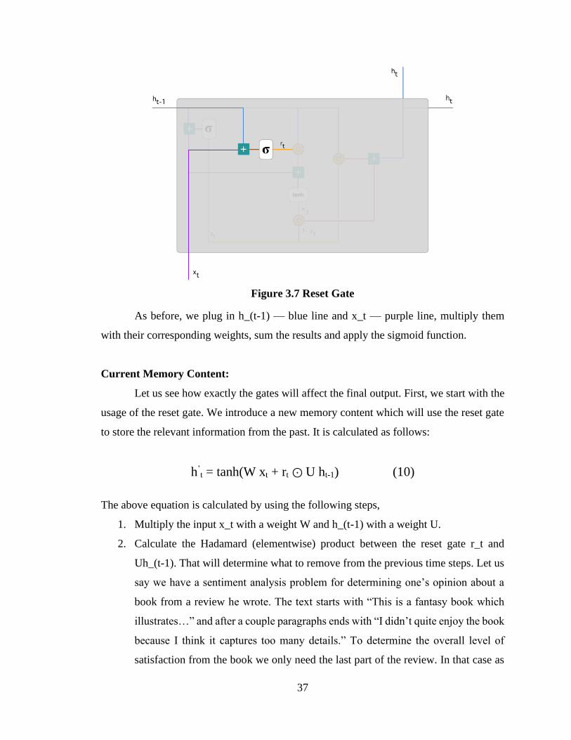
Figure 3.7 Reset Gate

As before, we plug in h_(t-1) — blue line and x_t — purple line, multiply them

with their corresponding weights, sum the results and apply the sigmoid function.

Current Memory Content:

Let us see how exactly the gates will affect the final output. First, we start with the

usage of the reset gate. We introduce a new memory content which will use the reset gate

to store the relevant information from the past. It is calculated as follows:

h’t = tanh(W xt + rt ⊙ U ht-1) (10)

The above equation is calculated by using the following steps,

1. Multiply the input x_t with a weight W and h_(t-1) with a weight U.

2. Calculate the Hadamard (elementwise) product between the reset gate r_t and

Uh_(t-1). That will determine what to remove from the previous time steps. Let us

say we have a sentiment analysis problem for determining one’s opinion about a

book from a review he wrote. The text starts with “This is a fantasy book which

illustrates…” and after a couple paragraphs ends with “I didn’t quite enjoy the book

because I think it captures too many details.” To determine the overall level of

satisfaction from the book we only need the last part of the review. In that case as

38

the neural network approaches to the end of the text it will learn to assign r_t vector

close to 0, washing out the past and focusing only on the last sentences.

3. Sum up the results of step 1 and 2.

4. Apply the nonlinear activation function tanh.

You can clearly see the steps in the Figure 14.

Figure 3.8 Current Memory Gate

We do an element-wise multiplication of h_(t-1) — blue line and r_t — orange line

and then sum the result — pink line with the input x_t — purple line. Finally, tanh is used

to produce h’_t — bright green line.

Final Memory at Current Time Step

As the last step, the network needs to calculate, h_t — vector which holds

information for the current unit and passes it down to the network. In order to do that the

update gate is needed. It determines what to collect from the current memory content —

h’_t and what from the previous steps — h_(t-1).

That is done as follows:

ht = zt ⊙ ht-1 + (1-zt) ⊙ h’t (11)

39

1. Apply element-wise multiplication to the update gate z_t and h_(t-1).

2. Apply element-wise multiplication to (1-z_t) and h’_t.

3. Sum the results from step 1 and 2.

Let us bring up the example about the book review. This time, the most relevant

information is positioned in the beginning of the text. The model can learn to set the vector

z_t close to 1 and keep most of the previous information. Since z_t will be close to 1 at this

time step, 1-z_t will be close to 0 which will ignore big portion of the current content (in

this case the last part of the review which explains the book plot) which is irrelevant for

our prediction. Here is an illustration in Figure 3.9 which emphasizes on the above

equation:

Figure 3.9 Final Memory Gate

Following through, you can see how z_t — green line is used to calculate 1-z_t

which, combined with h’_t — bright green line, produces a result in the dark red line. z_t

is also used with h_(t-1) — blue line in an element-wise multiplication. Finally, h_t — blue

line is a result of the summation of the outputs corresponding to the bright and dark red

lines.

Now, you can see how GRUs are able to store and filter the information using their

update and reset gates. That eliminates the vanishing gradient problem since the model is

not washing out the new input every single time but keeps the relevant information and

passes it down to the next time steps of the network. If carefully trained, they can perform

extremely well even in complex scenarios.

40

Training through Recurrent Neural Network

1. A single time step of the input is provided to the network.

2. Then calculate its current state using set of current input and the previous state.

3. The current ht becomes ht-1 for the next time step.

4. One can go as many time steps according to the problem and join the information

from all the previous states.

5. Once all the time steps are completed the final current state is used to calculate the

output.

6. The output is then compared to the actual output i.e the target output and the error

is generated.

7. The error is then backpropagated to the network to update the weights and hence

the network (RNN) is trained.

3.2 ADAM OPTIMIZER:

Gradient Descent is an iterative optimization algorithm, used to find the minimum

value for a function. The general idea is to initialize the parameters to random values, and

then take small steps in the direction of the “slope” at each iteration. Gradient descent is

highly used in supervised learning to minimize the error function and find the optimal

values for the parameters.

Adam is different to classical stochastic gradient descent. Stochastic gradient

descent maintains a single learning rate (termed alpha) for all weight updates and the

learning rate does not change during training. A learning rate is maintained for each

network weight (parameter) and separately adapted as learning unfolds. The method

computes individual adaptive learning rates for different parameters from estimates of first

and second moments of the gradients.

The authors describe Adam as combining the advantages of two other extensions

of stochastic gradient descent. Specifically:

• Adaptive Gradient Algorithm (AdaGrad) that maintains a per-parameter learning

rate that improves performance on problems with sparse gradients (e.g. natural

language and computer vision problems).

https://machinelearningmastery.com/learning-rate-for-deep-learning-neural-networks/

41

• Root Mean Square Propagation (RMSProp) that also maintains per-parameter

learning rates that are adapted based on the average of recent magnitudes of the

gradients for the weight (e.g. how quickly it is changing). This means the algorithm

does well on online and non-stationary problems (e.g. noisy).

Adam realizes the benefits of both AdaGrad and RMSProp. Instead of adapting the

parameter learning rates based on the average first moment (the mean) as in RMSProp,

Adam also makes use of the average of the second moments of the gradients (the

uncentered variance).Specifically, the algorithm calculates an exponential moving average

of the gradient and the squared gradient, and the parameters beta1 and beta2 control the

decay rates of these moving averages. The initial value of the moving averages and beta1

and beta2 values close to 1.0 (recommended) result in a bias of moment estimates towards

zero. This bias is overcome by first calculating the biased estimates before then calculating

bias-corrected estimates.

3.3 HYPER PARAMETERS

The hyperparameters used in the design of the Gated recurrent neural network have

a great impact on the performance of the network. Although there are many hyper-

parameters involved in the design of a Gated recurrent neural network, the parameters

having the largest impact on the performance of the network are learning rate, number of

hidden layers, number of units/cells in the hidden layer and the number of time-steps.

Learning Rate:

It is a measure of the rate at which the network optimizes the minimization of the

loss function in a neural network. Mathematically, if the loss function is L (X; W, b), then

the goal of the network is to minimize the loss (cost) function L. The weights are constantly

updated to achieve the best possible output reducing the loss value. The learning rate

determines how fast the parameters are updated. One must vary the learning rate during the

training of the neural network to obtain the best results.

Time-Steps:

Selecting the number of time-steps also plays a crucial role in the performance of

the system. The information required to find the correct patterns depends on the number of

time-steps that are required to back propagate. Tuning the number of time-steps improves

42

the output of the network. When more time-steps are selected, the network takes longer to

time to train and vice-versa.

Hidden Units:

The number of cells in a hidden layer determines the amount of computation

performed on the input data. The more hidden units in the network, the longer it takes to

train. The neural network should be trained for a various number of hidden units to verify

the performance of the system.

Hidden Layers:

The stacking of GRU layers makes a multilayer GRU, which has a great impact on

higher dimensional datasets. However, most deep neural networks obtain optimized

performance with a single hidden layer. One must decide on the number of hidden layers

to be used with respect to their data-set size and the dimensions.

Batch size:

Batch size is a term used in machine learning and refers to the number of training

examples utilized in one iteration. The batch size can be one of three options:

1. Batch mode: where the batch size is equal to the total dataset thus making the

iteration and epoch values equivalent.

2. Mini-batch mode: where the batch size is greater than one but less than the total

dataset size. Usually, a number that can be divided into the total dataset size.

3. Stochastic mode: where the batch size is equal to one. Therefore, the gradient and

the neural network parameters are updated after each sample.

Epoch:

In Deep Learning, an epoch is a hyperparameter which is defined before training a

model. One epoch is when an entire dataset is passed both forward and backward through

the neural network only once. Since one epoch is too big to feed to the computer at once

we divide it in several smaller batches.

1 Epoch = 1 Forward pass + 1 Backward pass for ALL training samples.

https://radiopaedia.org/articles/epoch-machine-learning?lang=us

43

Batch Size = Number of training samples in 1 Forward/1 Backward pass. With increase in

Batch size, required memory space increases. Iterations is the number of batches needed to

complete one epoch.

3.4. ACTIVATION FUNCTIONS

Neural network activation functions are a crucial component of deep learning.

Activation functions determine the output of a deep learning model, its accuracy, and the

computational efficiency of training a model—which can make or break a large-scale

neural network. Activation functions also have a major effect on the neural network’s

ability to converge and the convergence speed, or in some cases, activation functions might

prevent neural networks from converging in the first place. In a neural network, numeric

data points called inputs, are fed into the neurons in the input layer. Each neuron has a

weight and multiplying the input number with the weight gives the output of the neuron,

which is transferred to the next layer.

The activation function is a mathematical “gate” in between the input feeding the

current neuron and its output going to the next layer. It can be as simple as a step function

that turns the neuron output on and off, depending on a rule or threshold. Or it can be a

transformation that maps the input signals into output signals that are needed for the neural

network to function. Increasingly, neural networks use non-linear activation functions,

which can help the network learn complex data, compute, and learn almost any function

representing a question, and provide accurate predictions.

3 Types of Activation Functions

1. Binary Step Function

A binary step function is a threshold-based activation function. If the input

value is above or below a certain threshold, the neuron is activated and sends the

same signal to the next layer. The problem with a step function is that it does not

allow multi-value outputs—for example, it cannot support classifying the inputs

into one of several categories.

f (x) = {0 𝑖𝑓 𝑥 >= 0

1 𝑖𝑓 < 0 (12)

44

2. Linear Activation Function

A linear activation function takes the form:

A = cx (13)

It takes the inputs, multiplied by the weights for each neuron, and creates an output

signal proportional to the input. In one sense, a linear function is better than a step

function because it allows multiple outputs, not just yes and no. However, a linear

activation function has two major problems:

i. Not possible to use backpropagation (gradient descent) to train the

model—the derivative of the function is a constant, and has no

relation to the input, X. So, it is not possible to go back and

understand which weights in the input neurons can provide a better

prediction.

ii. All layers of the neural network collapse into one—with linear

activation functions, no matter how many layers in the neural

network, the last layer will be a linear function of the first layer

(because a linear combination of linear functions is still a linear

function). So, a linear activation function turns the neural network

into just one layer.

A neural network with a linear activation function is simply a linear

regression model. It has limited power and ability to handle complexity varying

parameters of input data.

3. Non-Linear Activation Functions

Modern neural network models use non-linear activation functions. They

allow the model to create complex mappings between the network’s inputs and

outputs, which are essential for learning and modelling complex data, such as

images, video, audio, and data sets which are non-linear or have high

dimensionality. Almost any process imaginable can be represented as a functional

computation in a neural network, provided that the activation function is non-linear.

45

Non-linear functions address the problems of a linear activation function:

i. They allow backpropagation because they have a derivative function which

is related to the inputs.

ii. They allow “stacking” of multiple layers of neurons to create a deep neural

network. Multiple hidden layers of neurons are needed to learn complex

data sets with high levels of accuracy.

Some common Nonlinear Activation Functions are as follows:

1. Sigmoid / Logistic

f(x) = sigmoid(x) = 1

1+𝑒−𝑥 (14)

This activation function translates the input ranged in [-Inf; +Inf] to the range

(0,1).

Advantages

• Smooth gradient, preventing “jumps” in output values.

• Output values bound between 0 and 1, normalizing the output of each

neuron.

• Clear predictions—For X above 2 or below -2, tends to bring the Y value

(the prediction) to the edge of the curve, very close to 1 or 0. This enables

clear predictions.

Disadvantages

• Vanishing gradient—for very high or very low values of X, there is almost

no change to the prediction, causing a vanishing gradient problem. This can

result in the network refusing to learn further or being too slow to reach an

accurate prediction.

• Outputs not zero centred.

• Computationally expensive

46

2. Tanh / Hyperbolic Tangent

tanh(x) = 2

1+𝑒−2𝑥 − 1 (15)

This activation function translates the input ranged in [-Inf; +Inf] to the range

(-1, 1).

Advantages

• Zero centred making it easier to model inputs that have strongly negative,

neutral, and strongly positive values.

• Otherwise like the Sigmoid function.

Disadvantages

• Like the Sigmoid function

3. ReLU (Rectified Linear Unit)

RELU (x) = {0 𝑖𝑓 𝑥 < 0

𝑥 𝑖𝑓 𝑥 ≥ 0 (16)

Advantages

• Computationally efficient—allows the network to converge very quickly

• Non-linear—although it looks like a linear function, ReLU has a derivative

function and allows for backpropagation

Disadvantages

• The Dying ReLU problem—when inputs approach zero, or are negative, the

gradient of the function becomes zero, the network cannot perform

backpropagation and cannot learn.

4.Softmax

𝜎(𝑧)𝑗 = 𝑒

𝑧𝑗

∑ 𝑒𝑧𝑘𝐾𝑘=1

(17)

where j = 1, 2, ..., K.

Advantages

• Able to handle multiple classes only one class in other activation

functions—normalizes the outputs for each class between 0 and 1, and

47

divides by their sum, giving the probability of the input value being in a

specific class.

• Useful for output neurons—typically Softmax is used only for the output

layer, for neural networks that need to classify inputs into multiple

categories.

3.5. EVALUATION MEASURES

In our model, the most important performance indicator (Accuracy, AC) of

intrusion detection is used to measure the performance of the RNN-IDS model. In addition

to the accuracy, we introduce the detection rate and false positive rate.

True Positive (TP): It is equivalent to those records that are correctly rejected, and it

denotes the number of anomaly records that are identified as anomaly.

False Positive (FP): It is the equivalent of incorrectly rejected, and it denotes the number

of normal records that are identified as anomaly.

True Negative (TN): It is equivalent to those correctly admitted, and it denotes the number

of normal records that are identified as normal.

False Negative (FN): It is equivalent to those incorrectly admitted, and it denotes the

number of anomaly records that are identified as normal.

We have the following notation:

Accuracy (AC): The percentage of the number of records classified correctly versus total

the records shown in (18).

AC =TP + TN

TP + TN + FP + FN (18)

True Positive Rate (TPR): As the equivalent of the Detection Rate (DR), it shows the

percentage of the number of records identified correctly over the total number of anomaly

records, as shown in (19).

TPR =TP

TP + FN (19)

48

False Positive Rate (FPR): The percentage of the number of records rejected incorrectly

is divided by the total number of normal records, as shown in (20).

FPR = FP

FP + TN (20)

Precision (PR): It is the fraction of data instances predicted as positive that are positive.

PR =TP

TP + FP (21)

F-Measure(F-score): It is also called F-score. It is used to evaluate the correctness of a

test. The F-Score is a measure that takes into consideration both the Precision and the

Recall in order to validate the accuracy. It is the harmonic mean of the Recall (DR) and the

Precision. Best results are achieved when F-measure equal to 1 and worst when F-measure

is 0 and it is expressed as follows:

F − score = 2 ∗(PR ∗ TPR)

(PR + TPR) (22)

The Confusion matrix visualizes the performance of the GRU-IDS model as shown

below.

Table 3.2 Confusion Matrix

49

4. EXPERIMENTAL ANALYSIS AND RESULTS

4.1 SYSTEM CONFIGURATION

4.1.1. Software Requirements

Programming Language: Python 3.7.

Libraries used: NumPy, Pandas, Matplotlib, TensorFlow.

GUI used: Anaconda Navigator.

Python:

Python is open source, interpreted, high level language and provides great approach

for object-oriented programming. It is one of the best languages used by data scientist for

various data science projects/application. Python provide great functionality to deal with

mathematics, statistics, and scientific function. It provides great libraries to deals with data

science application. One of the main reasons why Python is widely used in the scientific

and research communities is because of its ease of use and simple syntax which makes it

easy to adapt for people who do not have an engineering background. It is also more suited

for quick prototyping.

According to engineers coming from academia and industry, deep learning

frameworks available with Python APIs, in addition to the scientific packages have made

Python incredibly productive and versatile. There has been a lot of evolution in deep

learning Python frameworks and it is rapidly upgrading.

NumPy:

NumPy is Python library that provides mathematical function to handle large

dimension array. It provides various method/function for Array, Metrics, and linear

algebra. NumPy stands for Numerical Python. It provides lots of useful features for

operations on n-arrays and matrices in Python. The library provides vectorization of

mathematical operations on the NumPy array type, which enhance performance and speeds

up the execution. It’s very easy to work with large multidimensional arrays and matrices

using NumPy.

https://www.geeksforgeeks.org/python-numpy/

50

Pandas:

Pandas is one of the most popular Python libraries for data manipulation and

analysis. Pandas provide useful functions to manipulate large amount of structured data.

Pandas provide easiest method to perform analysis. It provides large data structures and

manipulating numerical tables and time series data. Pandas is a perfect tool for data

wrangling.

Pandas is designed for quick and easy data manipulation, aggregation, and

visualization. There two data structures in Pandas –

Series – It Handle and store data in one-dimensional data.

Data Frame – It Handle and store Two-dimensional data.

Matplotlib:

Matplotlib is another useful Python library for Data Visualization. Descriptive

analysis and visualizing data are very important for any organization. Matplotlib provides

various method to Visualize data in more effective way. Matplotlib allows to quickly make

line graphs, pie charts, histograms, and other professional grade figures. Using Matplotlib,

one can customize every aspect of a figure. Matplotlib has interactive features like zooming

and planning and saving the Graph in graphics format.

Anaconda:

Anaconda is a free and open-source distribution of the Python and R programming

languages for scientific computing that aims to simplify package management and

deployment. Package versions are managed by the package management system conda.

The Anaconda distribution includes data-science packages suitable for Windows, Linux,

and MacOS. Anaconda distribution comes with 1,500 packages selected from PyPI as well

as the conda package and virtual environment manager. It also includes a GUI, Anaconda

Navigator as a graphical alternative to the command line interface (CLI).

51

Anaconda Navigator:

Anaconda Navigator is a desktop graphical user interface (GUI) included in

Anaconda distribution that allows users to launch applications and manage conda

packages, environments and channels without using command-line commands. Navigator

can search for packages on Anaconda Cloud or in a local Anaconda Repository, install

them in an environment, run the packages and update them. It is available

for Windows, MacOS and Linux.

Jupyter Notebook:

The Jupyter Notebook is an open-source web application that allows you to create

and share documents that contain live code, equations, visualizations, and narrative text. A

Jupyter Notebook document is a JSON document, following a versioned schema, and

containing an ordered list of input/output cells which can contain code, text mathematics,

plots and rich media, usually ending with the “. ipynb" extension.

TensorFlow:

TensorFlow is an open-source software library for dataflow programming across a

range of tasks. It is a symbolic math library, and also used for machine learning applications

such as neural networks. Google open-sourced TensorFlow in November 2015. Since then,

TensorFlow has become the most starred machine learning repository on GitHub.

TensorFlow’s popularity is due to many things, but primarily because of the computational

graph concept, automatic differentiation, and the adaptability of the TensorFlow python

API structure. This makes solving real problems with TensorFlow accessible to most

programmers. Google’s TensorFlow engine has a unique way of solving problems. This

unique way allows for solving machine learning problems very efficiently.

TensorFlow, as the name indicates, is a framework to define and run computations

involving tensors. A tensor is a generalization of vectors and matrices to potentially higher

dimensions. Internally, TensorFlow represents tensors as n-dimensional arrays of base

datatypes. Each element in the Tensor has the same data type, and the data type is always

known. The shape (that is, the number of dimensions it has and the size of each dimension)

https://en.wikipedia.org/wiki/Graphical_user_interface

https://en.wikipedia.org/wiki/Command-line_interface

https://en.wikipedia.org/wiki/Windows

https://en.wikipedia.org/wiki/MacOS

https://en.wikipedia.org/wiki/Linux

52

might be only partially known. Most operations produce tensors of fully known shapes if

the shapes of their inputs are also fully known, but in some cases, it is only possible to find

the shape of a tensor at graph execution time.

Some of the basic tensorflow methods are:

i. tf. name_scope()

A context manager for use when defining a Python op.

tf.name_scope (

name

)

This context manager pushes a name scope, which will make the name of all

operations added within it have a prefix.

For example, to define a new Python op called my_op:

def my_op (a, b, c, name=None):

with tf.name_scope("MyOp") as scope:

a = tf.convert_to_tensor(a, name="a")

b = tf.convert_to_tensor(b, name="b")

c = tf.convert_to_tensor(c, name="c")

# Define some computation that uses `a`, `b`, and `c`.

return foo_op(..., name=scope)

When executed, the Tensors a, b, c, will have names MyOp/a, MyOp/b, and

MyOp/c. If the scope name already exists, the name will be made unique by

appending _n. For example, calling my_op the second time will generate

MyOp_1/a, etc.

Args:

• name: The prefix to use on all names created within the name scope.

Attributes:

• name

Raises:

• ValueError: If name is None, or not a string.

53

ii. tf.Session():

A class for running TensorFlow operations.

tf.Session(

target='', graph=None, config=None

)

A Session object encapsulates the environment in which Operation objects

are executed, and Tensor objects are evaluated. For example:

# Build a graph.

a = tf.constant(5.0)

b = tf.constant(6.0)

c = a * b

# Launch the graph in a session.

sess = tf.Session()

# Evaluate the tensor ‘c’.

print(sess.run(c))

A session may own resources, such as tf.Variable, tf.queue.QueueBase, and

tf.ReaderBase. It is important to release these resources when they are no longer

required. To do this, either invoke the tf.Session.close method on the session or use

the session as a context manager. The following two examples are equivalent:

# Using the `close()` method.

sess = tf.Session()

sess.run(...)

sess.close()

54

Args:

• target: (Optional.) The execution engine to connect to. Defaults to using an

in-process engine. See Distributed TensorFlow for more examples.

• graph: (Optional.) The Graph to be launched (described above).

• config: (Optional.) A ConfigProto protocol buffer with configuration

options for the session.

Attributes:

• graph: The graph that was launched in this session.

• graph_def: A serializable version of the underlying TensorFlow

• graph.sess_str: The TensorFlow process to which this session will connect.

iii. tf. placeholder():

Inserts a placeholder for a tensor that will be always fed.

tf.compat.v1.placeholder(

dtype, shape=None, name=None

)

x = tf.placeholder(tf.float32, shape=(1024, 1024))

y = tf.matmul(x, x)

with tf.Session() as sess:

print(sess.run(y)) # ERROR: will fail because x was not fed.

rand_array = np.random.rand(1024, 1024)

print(sess.run(y, feed_dict={x: rand_array})) # Will succeed.

Args:

• dtype: The type of elements in the tensor to be fed.

• shape: The shape of the tensor to be fed (optional). If the shape is not

specified, you can feed a tensor of any shape.

• name: A name for the operation (optional).

Returns:

• A Tensor that may be used as a handle for feeding a value, but not evaluated

directly.

Raises:

• RuntimeError: if eager execution is enabled

55

iv. tf. variable_scope():

A context manager for defining ops that creates variables (layers).

tf.variable_scope(

name_or_scope, default_name=None, values=None, initializer=None,

regularizer=None,caching_device=None,partitioner=None,custom_getter=None,

reuse=None, dtype=None, use_resource=None, constraint=None,

auxiliary_name_scope=True

)

This context manager validates that the (optional) values are from the same

graph, ensures that graph is the default graph, and pushes a name scope and a

variable scope. If name_or_scope is not None, it is used as is. If name_or_scope is

None, then default_name is used. In that case, if the same name has been previously

used in the same scope, it will be made unique by appending _N to it.

Variable scope allows you to create new variables and to share already

created ones while providing checks to not create or share by accident.

Simple example of how to create a new variable:

with tf..variable_scope("foo"):

with tf.variable_scope("bar"):

v = tf.get_variable("v", [1])

assert v.name == "foo/bar/v:0"

4.1.2. Hardware Requirements

CPU: Intel ® Core ™ i5-5200U CPU @ 2.20 GHz or above.

RAM: minimum 8 GB is required.

Operating System:

• Windows 8 or newer, 32 or 64 bit.

• Ubuntu 14+, 64 bit.

• macOS 10.13+ ,64 bit.

56

4.2 SAMPLE CODE ELABORATION:

4.2.1. Importing the required packages

import pandas as pd

import numpy as np

import tensorflow as tf

tf.reset_default_graph()

import matplotlib.pyplot as plt

from tensorflow.contrib import rnn

4.2.2. Loading the nsl-kdd datasets

train_data = pd.read_csv('nsl-kdd/kdd_train+.csv')

test_data = pd.read_csv('nsl-kdd/kdd_test+.csv')

Xtrain_input = train_data.iloc[:,:-1]

Ytrain_output = train_data.iloc[:,-1]

Xtest_input = test_data.iloc[:,:-1]

Ytest_output = test_data.iloc[:,-1]

4.2.3. Conversion of Symbolic features to Numerical values

training = pd.get_dummies(data=Xtrain_input, columns=['protocol_type', 'service',

'flag'])

testing = pd.get_dummies(data=Xtest_input, columns=['protocol_type', 'service',

'flag'])

traincols = list(training.columns.values)

testcols = list(testing.columns.values)

for col in traincols:

if col not in testcols:

testing[col] = 0

testcols.append(col)

for col in testcols:

if col not in traincols:

training[col] = 0

57

traincols.append(col)

l=[]

for i in range(len(Ytrain_output)):

if Ytrain_output[i] == 'normal':

l.append(1)

else:

l.append(0)

x_train = training

print(x_train.shape)

data={'labels': l}

y_train = pd.DataFrame(data)

print(y_train.shape)

l=[]

for i in range(len(Ytest_output)):

if Ytest_output[i] == 'normal':

l.append(1)

else:

l.append(0)

x_test = testing

print(x_test.shape)

data = {'labels':l}

y_test = pd.DataFrame(data)

print(y_test.shape)

4.2.4. Normalization

cols_to_normalise = list(training.columns.values)[:38]

training[cols_to_normalise] = training[cols_to_normalise].apply(lambda x: (x -

x.min()) / (x.max() - x.min()))

testing[cols_to_normalise] = testing[cols_to_normalise].apply(lambda x: (x -

x.min()) / (x.max() - x.min()))

58

training.replace(np.nan, 0, inplace=True)

testing.replace(np.nan, 0, inplace=True)

traincols = list(training.columns.values)

testcols = list(testing.columns.values)

for col in traincols:

if col not in testcols:

testing[col] = 0

testcols.append(col)

for col in testcols:

if col not in traincols:

training[col] = 0

traincols.append(col)

4.2.5. Feature Selection using Random forest classifier

sel = SelectFromModel(RandomForestClassifier(n_estimators = 100))

sel.fit(x_train, y_train.values.ravel())

selected_feat = x_train.columns[(sel.get_support())]

importances = sel.estimator_.feature_importances_

indices = np.argsort(importances)[::-1]

plt.figure()

plt.title("Feature importances")

plt.bar(range(x_train.shape[1]),importances[indices],color="r",align="center")

plt.xticks(range(x_train.shape[1]), indices)

plt.xlim([-1, x_train.shape[1]])

plt.show()

colnames = x_train.columns[(sel.get_support())]

def select_columns(data_frame, column_names):

new_frame = data_frame.loc[:, column_names]

return new_frame

x_train_reduced = select_columns(x_train,colnames)

x_test_reduced = select_columns(x_test,colnames)

59

X_train = np.array(x_train_reduced)

X_test = np.array(x_test_reduced)

Y_train = np.array(y_train)

Y_test = np.array(y_test)

y_train.columns = ["y1"]

y_train.loc[:,('y2')] = y_train['y1'] ==0

y_train.loc[:,('y2')] = y_train['y2'].astype(int)

Y_train = np.array(y_train)

y_test.columns = ["y1"]

y_test.loc[:,('y2')] = y_test['y1'] ==0

y_test.loc[:,('y2')] = y_test['y2'].astype(int)

Y_test = np.array(y_test)

4.2.6. Building the GRU-IDS model:

# Hyper Parameters

learning_rate = 0.001

training_epochs =180

display_step =1

num_layers = 1

input_dim=X_train.shape[1]

#Input Placeholders

with tf.name_scope('input'):

x = tf.placeholder(tf.float32,shape = [None,input_dim], name = "x-input")

y = tf.placeholder(tf.float32, shape = [None,2],name = "y-input")

#Weights and Biases

with tf.name_scope("weights"):

W = tf.Variable(tf.random_normal([input_dim,2]))

with tf.name_scope("biases"):

b = tf.Variable(tf.random_normal([2]))

60

#Model

with tf.name_scope("splitx"):

newx = tf.split(x,1,0)

with tf.name_scope("MultiRNNcell"):

multicell=tf.contrib.rnn.MultiRNNCell([tf.contrib.rnn.GRUCell(input_di

m) for i in range (num_layers)], state_is_tuple=True)

with tf.variable_scope('gru_cell'):

outputs,states = tf.contrib.rnn.static_rnn(multicell,newx,dtype=tf.float32,

scope = None)

with tf.name_scope("output"):

output = tf.add(tf.matmul(outputs[-1],W),b)

with tf.name_scope("cross_entropy"):

cost = tf.reduce_mean(tf.nn.softmax_cross_entropy_with_logits(labels = y,

logits = output))

with tf.name_scope("train"):

optimizer = tf.train.AdamOptimizer(learning_rate).minimize(cost)

with tf.name_scope("accuracy"):

correct_prediction = tf.equal(tf.argmax(output,1), tf.argmax(y,1))

cast = tf.cast(correct_prediction, tf.float32)

accuracy = tf.reduce_mean(cast)

#create summary for the cost and accuracy

tf.summary.scalar("cost",cost)

tf.summary.scalar("accuracy", accuracy)

summary_op = tf.summary.merge_all()

logs_path = "ids/gru/summary_data"

with tf.Session() as sess:

sess.run(tf.global_variables_initializer())

writer=tf.summary.FileWriter(logs_path,graph = tf.get_default_graph())

61

for i in range (training_epochs):

_,summary=sess.run([optimizer,summary_op],feed_dict={x:X_train,y:Y_t

rain})

writer.add_summary(summary,i)

if (i) % display_step == 0:

print(i,"Cost for this epoch is",sess.run(cost,feed_dict={x

:X_train,y:Y_train}))

print ("Accuracy",accuracy.eval(feed_dict = {x:X_test,y:Y_test}))

print ("test Output is :", sess.run(output,feed_dict = {x:X_test, y:Y_test}))

print ("test labels are :", sess.run(y,feed_dict = {x:X_test, y:Y_test}))

print ("train labels are :", sess.run(x,feed_dict = {x:X_train, y:Y_train}))

pred_class=sess.run(tf.argmax(output,1),feed_dict={x:X_test,y:Y_test})

labels_class = sess.run(tf.argmax(y,1),feed_dict = {x:X_test,y:Y_test})

conf=tf.contrib.metrics.confusion_matrix(labels_class,pred_class,dtype=

tf.int32)

print ("confusion matrix \n", sess.run(conf, feed_dict={x:X_test, y

:Y_test}))

n = tf.cast(labels_class,tf.int64)

TP = conf[0,0]

FN = conf [0,1]

FP = conf[1,0]

TN = conf[1,1]

#Accuracy

Acc = (TP+TN)/(TP+FP+TN+FN)

print ("Accuracy calculated through confusion matrix", sess.run (Acc,

feed_dict = {x:X_test,y:Y_test}))

# Precision

Precision = TP/(TP+FP)

print ("Precision\n",sess.run(Precision,feed_dict ={x:X_test, y:Y_test}))

62

#Recall

Recall = TP/(TP+FN)

print ("Recall (DR)\n", sess.run(Recall,feed_dict={x:X_test,y:Y_test}))

#F score

FScore = 2*((Precision*Recall)/(Precision+Recall))

print ("F1 Score is \n",sess.run(FScore,{x:X_test, y:Y_test}))

#False Alarm Rate

FAR = FP/(FP+TN)

print ("False Alarm Rate is \n",sess.run(FAR,feed_dict

={x:X_test,y:Y_test}))

63

4.3 SCREEN SHOTS

Figure 4.1 Performance of the GRU-IDS model on the training dataset if number of

epochs=30.

Figure 4.2 Performance of the GRU-IDS model on the test dataset if number of

epochs=30.

64


epochs=60.


epochs=60.

65


epochs=120.


epochs=120.

66


epochs=180.


epochs=180.

67


epochs=200.


epochs=200.

68

Figure 4.11 Performance of the GRU-IDS model on the training dataset if number

of epochs=360.


epochs=360.

69

4.4. EXPERIMENTAL ANALYSIS

Table 4.1 Performance measures of existing systems.

IDS SYSTEM Validation Accuracy Test Accuracy

SVM 99.55% 78.32%

KNN 99.42% 73.26%

NB 89.32% 75.62%

RF 99.73% 83.92%

ANN 99.49% 84.17%

RNN 97.53% 82.74%

LSTM 98.12% 85.42%

Table 4.2 Performance measures of the proposed system

Epochs Validation Accuracy Test Accuracy

30 80.19% 76.78%

60 94.74% 88.69%

120 95.90% 89.22%

180 96.43% 90.13%

200 96.60% 89.84 %

360 98.10% 90.06%

70

5. CONCLUSION AND FUTURE WORK

5.1. CONCLUSION

In this study, we designed a new Intrusion Detection System. We propose a new

model which uses GRUs as the main memory unit, combined with a Random Forest

Classifier as a feature selection method to identify network intrusions. Deep learning

techniques were used for training and achieved good performance. Experiments on the

well-known NSL-KDD dataset showed that the system has leading performance. The

overall detection rate was 96.89% on NSL-KDD, with false positive rates as low as 0.03%

and 0.1%, respectively. The experimental results show an accuracy rate of 98.10% on the

training dataset and 90.06% on the test dataset. This model outperforms all the other

existing Intrusion Detection Systems.

5.2. FUTURE WORK

In our future works, we intend to study the performance of individual classes of

attacks in the NSLKDD dataset using the GRU-IDS model. The next step could be to

optimize the system so that it can be applied to real network environments and be

implemented more efficiently and focus on decreasing the time complexity and increasing

the accuracy rate in detecting intrusions in a network.

71

6. REFERENCES

[1] Revathi S, Malathi A. A detailed analysis of NSL-KDD dataset using various machine

learning techniques for intrusion detection. International Journal of Engineering Research

& Technology (IJERT). 2013 Dec;2(12):1848-53.

[2] Bhupendra I, Yadav A. Performance analysis of NSL-KDD dataset using ANN. In 2015

international conference on signal processing and communication engineering systems

2015 Jan 2(pp. 92-96),IEEE.

[3] Shrivas AK, Dewangan AK. An ensemble model for classification of attacks with

feature selection based on KDD99 and NSL-KDD data set. International Journal of

Computer Applications.2014;99(15):8-13.

[4] Chae HS, Jo BO, Choi SH, Park TK. Feature selection for intrusion detection using

NSL-KDD. Recent advances in computer science.2013 Nov:184-7.

[5] Kasongo SM, Sun Y.A Deep Long Short-Term Memory based classifier for Wireless

Intrusion Detection System. ICT Express. 2019 Aug 22.

[6] Kasongo SM, Sun Y.A deep learning method with a filter-based feature engineering

for the wireless intrusion detection system. IEEE Access. 2019 Mar 18; 7:38597-607.

[7] Dhanabal L, Shantharajah SP. A study on NSL-KDD dataset for intrusion detection

system based on classification algorithms. International Journal of Advanced Research in

Computer and Communication Engineering. 2015 Jun;4(6):446-52.

[8] Farnaaz N,Jabbar M A.Random forest modeling for network intrusion detection system.

Procedia Computer Science.2016 Jan 1;89(1):213-7.

72

[9] Bhavsar YB, Waghmare KC. Intrusion detection system using data mining technique:

Support vector machine. International Journal of Emerging Technology and Advanced

Engineering. 2013 Mar;3(3):581-6.

[10] KS D, Ramakrishna BB. An artificial neural network-based intrusion detection system

and classification of attacks. International Journal of Engineering Research and

Applications. 2013.

[11] J. Kim, H. Kim, An effective intrusion detection classifier using longshort-term

memory with gradient descent optimization, in: IEEE Int. Conf. on Platform Technology

and Service, 2017, pp. 1–6.

[12] Yin C, Zhu Y, Fei J, He X. A deep learning approach for intrusion detection using

recurrent neural networks. IEEE Access.2017 Oct 12;5:21954-61.

[13] Sharma S, Gupta R K. Intrusion detection system: A review. International Journal of

Security and its Applications.2015;9(5):69-76.

[14] Allen J, Christie A, Fithen W, McHugh J, Picket J. State of the practice of intrusion

detection technologies. CARNEGIE-MELLON UNIV PITTSBURGH PA SOFTWARE

ENGINEERING INST; 2000 Jan.

[15] Reddy RR, Ramadevi Y, Sunitha KN. Effective discriminant function for intrusion

detection using SVM.in 2016 International Conference on Advances in Computing.

Communications and informatics (ICACCI) 2016 Sep 21(pp.1148-1153). IEEE.

[16] Li W, Yi P, Wu Y, Pan L, Li J.A new intrusion detection system based on KNN

classification algorithm in the wireless sensor network. Journal of Electrical and Computer

Engineering 2014.

73

[17] Sahu S, Mehtre BM. Network intrusion detection system using J48 Detection Tree. In

2015 International Conference on Advances in Computing, Communications, and

Informatics (ICACCI) 2015 Aug 10(pp. 2023-2026). IEEE.

[18] Ashraf N, Ahmad W, Ashraf R. A comparative study of data mining algorithms for

high detection rate in intrusion detection system. Annals of Emerging Technologies in

Computing (AETiC), Print ISSN. 2018:2516-0281.

74

APPENDICES

BASE PAPER

Received September 5, 2017, accepted October 5, 2017, date of publication October 12, 2017, date of current version November 7, 2017.

Digital Object Identifier 10.1109/ACCESS.2017.2762418

A Deep Learning Approach for IntrusionDetection Using Recurrent Neural NetworksCHUANLONG YIN , YUEFEI ZHU, JINLONG FEI, AND XINZHENG HEState Key Laboratory of Mathematical Engineering and Advanced Computing, Zhengzhou 450001, China

Corresponding author: Chuanlong Yin ([email protected])

This work was supported by the National Key Research and Development Program of China under Grant 2016YFB0801601and 2016YFB0801505.

ABSTRACT Intrusion detection plays an important role in ensuring information security, and the keytechnology is to accurately identify various attacks in the network. In this paper, we explore how to modelan intrusion detection system based on deep learning, and we propose a deep learning approach for intrusiondetection using recurrent neural networks (RNN-IDS). Moreover, we study the performance of the model inbinary classification and multiclass classification, and the number of neurons and different learning rateimpacts on the performance of the proposed model. We compare it with those of J48, artificial neuralnetwork, random forest, support vector machine, and other machine learning methods proposed by previousresearchers on the benchmark data set. The experimental results show that RNN-IDS is very suitable formodeling a classification model with high accuracy and that its performance is superior to that of traditionalmachine learning classification methods in both binary and multiclass classification. The RNN-IDS modelimproves the accuracy of the intrusion detection and provides a new research method for intrusion detection.

INDEX TERMS Recurrent neural networks, RNN-IDS, intrusion detection, deep learning, machine learning.

I. INTRODUCTIONWith the increasingly deep integration of the Internet andsociety, the Internet is changing the way in which peoplelive, study and work, but the various security threats thatwe face are becoming more and more serious. How to iden-tify various network attacks, especially unforeseen attacks,is an unavoidable key technical issue. An Intrusion DetectionSystem (IDS), a significant research achievement in the infor-mation security field, can identify an invasion, which could bean ongoing invasion or an intrusion that has already occurred.In fact, intrusion detection is usually equivalent to a classifi-cation problem, such as a binary or a multiclass classificationproblem, i.e., identifying whether network traffic behaviouris normal or anomalous, or a five-category classificationproblem, i.e., identifying whether it is normal or any one ofthe other four attack types: Denial of Service (DOS), Userto Root (U2R), Probe (Probing) and Root to Local (R2L).In short, the main motivation of intrusion detection is toimprove the accuracy of classifiers in effectively identifyingthe intrusive behaviour.

Machine learning methodologies have been widely usedin identifying various types of attacks, and a machine learn-ing approach can help the network administrator take the

corresponding measures for preventing intrusions.However, most of the traditional machine learning method-ologies belong to shallow learning and often emphasizefeature engineering and selection; they cannot effectivelysolve the massive intrusion data classification problem thatarises in the face of a real network application environment.With the dynamic growth of data sets, multiple classificationtasks will lead to decreased accuracy. In addition, shallowlearning is unsuited to intelligent analysis and the forecastingrequirements of high-dimensional learningwithmassive data.In contrast, deep learners have the potential to extract betterrepresentations from the data to create much better models.As a result, intrusion detection technology has experiencedrapid development after falling into a relatively slow period.

After Professor Hinton [1] proposed the theory of deeplearning in 2006, deep learning theory and technology under-went a meteoric rise in the field of machine learning.In this scenario, relevant theoretical papers and practicalresearch findings emerged endlessly and produced remark-able achievements, especially in the fields of speech recog-nition, image recognition [2] and action recognition [3]–[5].The fact that deep learning theory and technology has hada very rapid development in recent years means that a new

219542169-3536 2017 IEEE. Translations and content mining are permitted for academic research only.

Personal use is also permitted, but republication/redistribution requires IEEE permission.See http://www.ieee.org/publications_standards/publications/rights/index.html for more information.

VOLUME 5, 2017

https://orcid.org/0000-0003-0735-9019

C. Yin et al.: Deep Learning Approach for Intrusion Detection Using Recurrent Neural Networks

era of artificial intelligence has opened and offered a com-pletely new way to develop intelligent intrusion detectiontechnology.

Due to growing computational resources, recurrent neuralnetworks (RNNs) (which have been around for decades buttheir full potential has only recently started to become widelyrecognized, such as convolutional neural networks (CNNs))have recently generated a significant development in thedomain of deep learning [6]. In recent years, RNNs haveplayed an important role in the fields of computer vision,natural language processing (NLP), semantic understanding,speech recognition, language modelling, translation, picturedescription, and human action recognition [7]–[9], amongothers.

Because deep learning has the potential to extract betterrepresentations from the data to create much better models,and inspired by recurrent neural networks, we have proposeda deep learning approach for an intrusion detection systemusing recurrent neural networks (RNN-IDS). The main con-tributions of this paper are summarized as follows.

(1) We present the design and implementation of the detec-tion system based on recurrent neural networks. Moreover,we study the performance of the model in binary classifica-tion and multiclass classification, and the number of neuronsand different learning rate impacts on the accuracy.

(2) By contrast, we study the performance of the naivebayesian, random forest, multi-layer perceptron, support vec-tor machine and other machine learning methods in multi-class classification on the benchmark NSL-KDD dataset.

(3) We compare the performance of RNN-IDS with othermachine learning methods both in binary classification andmulticlass classification. The experimental results illustratethat RNN-IDS is very suitable for intrusion detection. Theperformance of RNN-IDS is superior to the traditional clas-sification method on the NSL-KDD dataset in both binaryand multiclass classification, and it improves the accuracy ofintrusion detection, thus providing a new research method forintrusion detection.

The remainder of this paper is organized as follows.In Section II, we review the related research in the field ofintrusion detection, especially how deep learning methodsfacilitate the development of intrusion detection. A descrip-tion of a RNN-based IDS architecture and the performanceevaluation measures are introduced in Section III. Section IVhighlights RNN-IDS with a discussion about the experimen-tal results and a comparison with a few previous studies usingthe NSL-KDD dataset. Finally, the conclusions are discussedin Section V.

II. RELEVANT WORKIn prior studies, a number of approaches based on tra-ditional machine learning, including SVM [10], [11],K-Nearest Neighbour (KNN) [12], ANN [13], Random For-est (RF) [14], [15] and others [16], [17], have been pro-posed and have achieved success for an intrusion detectionsystem.

In recent years, deep learning, a branch of machine learn-ing, has become increasingly popular and has been appliedfor intrusion detection; studies have shown that deep learningcompletely surpasses traditional methods. In [18], the authorsutilize a deep learning approach based on a deep neural net-work for flow-based anomaly detection, and the experimentalresults show that deep learning can be applied for anomalydetection in software defined networks. In [19], the authorspropose a deep learning based approach using self-taughtlearning (STL) on the benchmark NSL-KDD dataset in anetwork intrusion detection system. When comparing its per-formance with those observed in previous studies, the methodis shown to be more effective. However, this category ofreferences focuses on the feature reduction ability of thedeep learning. It mainly uses deep learning methods for pre-training, and it performs classification through the traditionalsupervision model. It is not common to apply the deep learn-ing method to perform classification directly, and there is alack of study of the performance in multiclass classification.

According to [20], RNNs are considered reduced-size neu-ral networks. In that paper, the author proposes a three-layer RNN architecture with 41 features as inputs and fourintrusion categories as outputs, and for misuse-based IDS.However, the nodes of layers are partially connected,the reduced RNNs do not show the ability of deep learn-ing to model high-dimensional features, and the authorsdo not study the performance of the model in the binaryclassification.

With the continuous development of big data and comput-ing power, deep learning methods have blossomed rapidly,and have been widely utilized in various fields. Followingthis line of thinking, a deep learning approach for intrusiondetection using recurrent neural networks (RNN-IDS) is pro-posed in this paper. Compared with previous works, we usethe RNN-based model for classification rather than for pre-training. Besides, we use the NSL-KDD dataset with a sep-arate training and testing set to evaluate their performancesin detecting network intrusions in both binary and multiclassclassification, and we compare it with J48, ANN, RF, SVMand other machine learning methods proposed by previousresearchers.

III. PROPOSED METHODOLOGIESRecurrent neural networks include input units, output unitsand hidden units, and the hidden unit completes the mostimportant work. The RNN model essentially has a one-wayflow of information from the input units to the hidden units,and the synthesis of the one-way information flow from theprevious temporal concealment unit to the current timinghiding unit is shown in Fig. 1. We can regard hidden units asthe storage of the whole network, which remember the end-to-end information. When we unfold the RNN, we can findthat it embodies the deep learning. A RNNs approach can beused for supervised classification learning.

Recurrent neural networks have introduced a directionalloop that can memorize the previous information and apply

VOLUME 5, 2017 21955


FIGURE 1. Recurrent Neural Networks (RNNs).

FIGURE 2. Block diagram of proposed RNN-IDS.

it to the current output, which is the essential differencefrom traditional Feed-forward Neural Networks (FNNs). Thepreceding output is also related to the current output of asequence, and the nodes between the hidden layers are nolonger connectionless; instead, they have connections. Notonly the output of the input layer but also the output of thelast hidden layer acts on the input of the hidden layer.

The step involved in RNN-IDS is shown in Fig. 2.

A. DATASET DESCRIPTIONThe NSL-KDD dataset [21], [22] generated in 2009 is widelyused in intrusion detection experiments. In the latest liter-ature [23]–[25], all the researchers use the NSL-KDD asthe benchmark dataset, which not only effectively solvesthe inherent redundant records problems of the KDD Cup1999 dataset but also makes the number of records reasonablein the training set and testing set, in such a way that the classi-fier does not favour more frequent records. The dataset coversthe KDDTrain+ dataset as the training set and KDDTest+ andKDDTest−21 datasets as the testing set, which has different

TABLE 1. Different classifications in the NSL-KDD dataset.

TABLE 2. Features of NSL-KDD dataset.

normal records and four different types of attack records,as shown in Table 1. The KDDTest−21 dataset is a subset ofthe KDDTest+ and is more difficult for classification.There are 41 features and 1 class label for every traf-

fic record, and the features include basic features (No.1-No.10), content features (No.11 - No.22), and traffic features(No.23 - No.41) as shown in Table 2. According to theircharacteristics, attacks in the dataset are categorized into fourattack types: DoS (Denial of Service attacks), R2L (Root toLocal attacks), U2R (User to Root attack), and Probe (Prob-ing attacks). The testing set has some specific attack typesthat disappear in the training set, which allows it to provide amore realistic theoretical basis for intrusion detection.

B. DATA PREPROCESSING1) NUMERICALIZATIONThere are 38 numeric features and 3 nonnumeric fea-tures in the NSL-KDD dataset. Because the input value ofRNN-IDS should be a numeric matrix, we must convert somenonnumeric features, such as ‘protocol_type’, ‘service’ and‘flag’ features, into numeric form. For example, the feature‘protocol_type’ has three types of attributes, ‘tcp’, ‘udp’,and ‘icmp’, and its numeric values are encoded as binary

21956 VOLUME 5, 2017


vectors (1,0,0), (0,1,0) and (0,0,1). Similarly, the feature‘service’ has 70 types of attributes, and the feature ‘flag’has 11 types of attributes. Continuing in this way, 41-dimensional features map into 122-dimensional features aftertransformation.

2) NORMALIZATIONFirst, according to some features, suchas ‘duration[0,58329]’,‘src_bytes[0,1.3 × 109]’ and ‘dst_bytes[0,1.3 × 109]’,where the difference between the maximum and minimumvalues has a very large scope, we apply the logarithmicscaling method for scaling to obtain the ranges of ‘dura-tion[0,4.77]’, ‘src_bytes[0,9.11]’ and ‘dst_bytes[0,9.11]’.Second, the value of every feature is mapped to the [0,1] rangelinearly according to (1), where Max denotes the maximumvalue and Min denotes minimum value for each feature.

xi =xi −MinMax −Min

(1)

C. METHODOLOGYIt is obvious that the training of the RNN-IDS model consistsof two parts - Forward Propagation and Back Propagation.Forward Propagation is responsible for calculating the out-put values, and Back Propagation is responsible for passingthe residuals that were accumulated to update the weights,which is not fundamentally different from the normal neuralnetwork training.

FIGURE 3. The unfolded Recurrent Neural Network.

According to Fig. 1, an unfolded recurrent neural networkis presented in Fig. 3. The standard RNN is formalized as fol-lows: Given training samples xi(i = 1, 2, . . ., m), a sequenceof hidden states hi (i = 1, 2, . . ., m), and a sequence ofpredictions yi(i = 1, 2, . . ., m). Whx is the input-to-hiddenweight matrix, Whh is the hidden-to-hidden weight matrix,Wyh is the hidden-to-output weight matrix, and the vectors bhand by are the biases [26]. The activation function e is a sig-moid, and the classification function g engages the SoftMaxfunction.

Refer to Fig. 3 and [26], Forward Propagation AlgorithmandWeights Update Algorithm are described as Algorithms 1and 2 respectively.

The objective function associated with RNNs for a singletraining pair (xi, yi) is defined as f(θ ) =L(yi : yi) [26],where L is a distance function which measures the deviationof the predictions yi from the actual labels yi. Let η be thelearning rate and k be the number of current iterations. Givena sequence of labels yi(i = 1, 2, . . ., m).

Algorithm 1 Forward Propagation AlgorithmInput xi(i = 1, 2, . . ., m)Output yi1: for i from 1 to m do2: tι =Whxxi +Whhhi−1+bh3: hi = sigmoid (ti)4: si =Wyhhi+by5: yi = SoftMax (si)6: end for

Algorithm 2 Weights Update AlgorithmInput 〈yi, yi〉(i = 1, 2, . . ., m)Initialization θ = {Whx ,Whh, Wyh, bh, by}Output θ = {Whx ,Whh,Wyh, bh, by}1: for i from k downto 1 do2: Calculate the cross entropy between theoutput value and the label value: L(yi: yi) ← -∑

i∑

j yij log (yij)+ (1− yij) log(1− yij)3: Compute the partial derivative with respect to θi :δi← dL/dθi4: Weight update: θi← θiη + δi5: end for

D. EVALUATION METRICSIn our model, the most important performance indica-tor (Accuracy, AC) of intrusion detection is used to measurethe performance of the RNN-IDS model. In addition to theaccuracy, we introduce the detection rate and false positiverate. The True Positive (TP) is equivalent to those correctlyrejected, and it denotes the number of anomaly records thatare identified as anomaly. The False Positive (FP) is theequivalent of incorrectly rejected, and it denotes the numberof normal records that are identified as anomaly. The TrueNegative (TN) is equivalent to those correctly admitted, andit denotes the number of normal records that are identified asnormal. The False Negative (FN) is equivalent to those incor-rectly admitted, and it denotes the number of anomaly recordsthat are identified as normal. Table 3 shows the definition ofconfusion matrix. We have the following notation:

Accuracy: the percentage of the number of records classi-fied correctly versus total the records shown in (2).

AC =TP+ TN

TP+ TN+ FP+ FN(2)

True Positive Rate (TPR): as the equivalent of the Detec-tion Rate (DR), it shows the percentage of the number ofrecords identified correctly over the total number of anomalyrecords, as shown in (3).

TPR =TP

TP+ FN(3)

False Positive Rate (FPR): the percentage of the number ofrecords rejected incorrectly is divided by the total number of

VOLUME 5, 2017 21957


TABLE 3. Confusion matrix.

normal records, as shown in (4).

FPR =FP

FP+ TN(4)

Hence, the motivation for the IDS is to obtain a higheraccuracy and detection rate with a lower false positive rate.

IV. EXPERIMENT RESULTS AND DISCUSSIONIn this research, we have used one of the most current andbroadest deep learning frameworks - Theano [27]. The exper-iment is performed on a personal notebook ThinkPad E450,which has a configuration of an Intel Core i5-5200U [email protected] GHz, 8 GB memory and does not use GPU accel-eration. Two experiments have been designed to study theperformance of the RNN-IDS model for binary classifica-tion (Normal, anomaly) and five-category classification, suchas Normal, DoS, R2L, U2R and Probe. In order to comparewith other other machine learning methods, contrast experi-ments are designed at the same time. In the binary classifica-tion experiments, we have compared the performance with anANN, naive Bayesian, random forest, multi-layer perceptron,support vector machine and other machine learning methods,as mentioned in [13] and [21]. In the same way, we analysethe multi-classification of the RNN-IDS model based on theNSL-KDD dataset. By contrast, we study the performanceof the ANN, naive Bayesian, random forest, multi-layer per-ceptron, support vector machine and other machine learningmethods in the five-category classification. Finally, we com-pare the performance of the RNN-IDS model with traditionalmethods. Furthermore, we construct the dataset refer to [20]and compare the performance with the reduced-size RNNmethod.

A. BINARY CLASSIFICATIONIn Sec B, we have mapped 41-dimensional features into122-dimensional features, thus the RNN-IDS model has 122input nodes, and 2 output nodes in the binary classificationexperiments. The number of epochs are given 100. To trainthe better model, let the number of hidden nodes be 20,60, 80, 120, and 240 respectively, the learning rate be 0.01,0.1 and 0.5 respectively, then we observe the classificationaccuracy on the NSL-KDD dataset as shown in Table 4. Thedifferent results we obtain show that the accuracy is relate tothe number of hidden nodes and the learning rate.

In our experiment, the model gets a higher accuracy,when there are 80 hidden nodes and the learning rate is 0.1.Table 5 shows the confusion matrix of the RNN-IDS on the

TABLE 4. The accuracy and training time (second) of RNN-IDS withdifferent learning rate and hidden nodes.

TABLE 5. Confusion matrix of 2-category classification on KDDTEST+.

testing set KDDTest+ in the 2-category classification exper-iments. The experiments show that RNN-IDS works with agood detection rate (83.28%) when given 100 epochs for theKDDTrain+ dataset. We obtain 68.55% for the KDDTest−21

dataset and 99.81% for the KDDTrain+ dataset as shownin Fig. 4.

In [21], the authors have shown the results obtained by J48,Naive Bayesian, Random Forest, Multi-layer Perceptron,Support Vector Machine and the other classification algo-rithms, and the artificial neural network algorithm also gives81.2% in [13], which is the recent literature about ANNalgorithms applied in the filed of intrusion detection. Fortu-nately, these results are all based on the same benchmark - theNSL-KDD dataset. Obviously, the performance of RNN-IDSmodel is superior to other classification algorithms in binaryclassification as shown in Fig. 5.

B. MULTICLASS CLASSIFICATIONIn the five-category classification experiments, we find thatthe model has higher accuracy on the KDDTest+ when thereare 80 hidden nodes in the RNN-IDS model, meanwhile the

21958 VOLUME 5, 2017


FIGURE 4. The Accuracy on the KDDTest+ and KDDTest−21 datasets in theBinary Classification.

FIGURE 5. Performance of RNN-IDS and the other models in the binaryclassification.

learning rate is 0.5, and the training is performed 80 timesfrom Table 6.

In order to compare the performance of different classi-fication algorithms on the benchmark dataset for the multi-calss classification as the binary classification experimentsJ48, Naive Bayesian, Random Forest, Multi-layer Percep-tron, Support Vector Machine and other machine learningalgorithms are used to train models through the trainingset (using 10-layer cross-validation) by mean of the open-sourcemachine learning and datamining softwareWeka [28].We then apply the models to the testing set. The results aredescribed in Fig. 6. Compared with the binary classification,the accuracy of classification algorithms is declined in thefive-category classification.

Table 7 shows the confusion matrix of the RNN-IDS onthe test set KDDTest+ in the five-category classificationexperiments. The experiment shows that the accuracy of themodel is 81.29% for the test set KDDTest+ and 64.67% forKDDTest−21, which is better than those obtained using J48,

TABLE 6. The accuracy and training time (second) of RNN-IDS withdifferent learning rate and hidden nodes.

FIGURE 6. Performance of RNN-IDS and the other models in thefive-category classification.

naive bayes, random forest, multi-layer perceptron and theother classification algorithms. In addition, it is better than theartificial neural network algorithm on the test set KDDTest+,which obtained 79.9% in the literature [13]. Table 8 showsthe detection rate and false positive rate of the different attacktypes.

In order to compare the performance of RNN-IDS withthe reduced-size RNN method proposed in [20], we con-structed the training set and testing set from KDD CUP1999 dataset according to the paper. The training and testing

VOLUME 5, 2017 21959


TABLE 7. Confusion matrix for the five-category experiments onKDDTest+.

TABLE 8. Results of the evaluation metrics for the five-categoryclassification.

TABLE 9. Different classifications in the training and testing sets

sets are described in detail in Table 9. In this experiment,the detection rate of the RNN-IDS model gets 97.09% on thetesting dataset, not only higher than the detection rate on theNSL-KDD dataset, but also higher than 94.1% in the lit-erature [20]. The experimental results show that the fullyconnected model has stronger modeling ability and higherdetection rate than the reduced-size RNN model. The train-ing of our model (20 hidden nodes, the learning rate is0.1, and epochs are 50) spends 1765 seconds without anyGPU acceleration, which more than 1383 seconds in theliterature [20].

C. DISCUSSIONBased on the same benchmark, using KDDTrain+ as thetraining set and KDDTest+ and KDDTest−21 as the test-ing set, the experimental results show that for both binaryand multiple classification, the intrusion detection model ofRNN-IDS training through the training set has higher accu-racy than the other machine learningmethods andmaintains ahigh accuracy rate, even in the case of multiple classification.Of course, the model we proposed will spend more time for

training, but using GPU acceleration can reduce the trainingtime.

V. CONCLUSIONSThe RNN-IDS model not only has a strong modelling abilityfor intrusion detection, but also has high accuracy in bothbinary and multiclass classification. Compared with tradi-tional classification methods, such as J48, naive bayesian,and random forest, the performance obtains a higher accu-racy rate and detection rate with a low false positive rate,especially under the task of multiclass classification on theNSL-KDD dataset. The model can effectively improve boththe accuracy of intrusion detection and the ability to recognizethe intrusion type. Of course, in the future research, we willstill pay attention to reduce the training time using GPUacceleration, avoid exploding and vanishing gradients, andstudy the classification performance of LSTM, BidirectionalRNNs algorithm in the field of intrusion detection.

REFERENCES[1] Y. LeCun, Y. Bengio, and G. Hinton, ‘‘Deep learning,’’ Nature, vol. 521,

no. 7553, pp. 436–444, May 2015.[2] J. Schmidhuber, ‘‘Deep learning in neural networks: An overview,’’Neural

Netw., vol. 61, pp. 85–117, Jan. 2015.[3] L. Liu, L. Shao, X. Li, and K. Lu, ‘‘Learning spatio-temporal represen-

tations for action recognition: A genetic programming approach,’’ IEEETrans. Cybern., vol. 46, no. 1, pp. 158–170, Jan. 2016.

[4] A.-A. Liu, Y.-T. Su, W.-Z. Nie, and M. Kankanhalli, ‘‘Hierarchical cluster-ing multi-task learning for joint human action grouping and recognition,’’IEEE Trans. Pattern Anal. Mach. Intell., vol. 39, no. 1, pp. 102–114,Jan. 2017.

[5] J. Wu, Y. Zhang, and W. Lin, ‘‘Good practices for learning to recognizeactions using FV and VLAD,’’ IEEE Trans. Cybern., vol. 46, no. 12,pp. 2978–2990, Dec. 2016.

[6] A. Karpathy. (2015). The unreasonable effectiveness of recurrentneural networks. Andrej Karpathy Blog. [Online]. Available: http://karpathy.github.io/2015/05/21/rnn-effectiveness/

[7] X. Peng, L. Wang, X. Wang, and Y. Qiao, ‘‘Bag of visual words and fusionmethods for action recognition: Comprehensive study and good practice,’’Comput. Vis. Image Understand., vol. 150, pp. 109–125, Sep. 2016.

[8] A.-A. Liu, Y.-T. Su, P.-P. Jia, Z. Gao, T. Hao, and Z.-X. Yang,‘‘Multiple/single-view human action recognition via part-induced mul-titask structural learning,’’ IEEE Trans. Cybern., vol. 45, no. 6,pp. 1194–1208, Jun. 2015.

[9] W. Nie, A. Liu, W. Li, and Y. Su, ‘‘Cross-view action recognition by cross-domain learning,’’ Image Vis. Comput., vol. 55, pp. 109–118, Nov. 2016.

[10] F. Kuang,W. Xu, and S. Zhang, ‘‘A novel hybrid KPCA and SVMwith GAmodel for intrusion detection,’’ Appl. Soft Comput., vol. 18, pp. 178–184,May 2014.

[11] R. R. Reddy, Y. Ramadevi, and K. V. N. Sunitha, ‘‘Effective discriminantfunction for intrusion detection using SVM,’’ in Proc. Int. Conf. Adv.Comput., Commun. Inform. (ICACCI), Sep. 2016, pp. 1148–1153.

[12] W. Li, P. Yi, Y. Wu, L. Pan, and J. Li, ‘‘A new intrusion detection sys-tem based on KNN classification algorithm in wireless sensor network,’’J. Elect. Comput. Eng., vol. 2014, Jun. 2014, Art. no. 240217.

[13] B. Ingre and A. Yadav, ‘‘Performance analysis of NSL-KDD dataset usingANN,’’ in Proc. Int. Conf. Signal Process. Commun. Eng. Syst., Jan. 2015,pp. 92–96.

[14] N. Farnaaz and M. A. Jabbar, ‘‘Random forest modeling for networkintrusion detection system,’’ Procedia Comput. Sci., vol. 89, pp. 213–217,Jan. 2016.

[15] J. Zhang, M. Zulkernine, and A. Haque, ‘‘Random-forests-based networkintrusion detection systems,’’ IEEE Trans. Syst., Man, Cybern. C, Appl.Rev., vol. 38, no. 5, pp. 649–659, Sep. 2008.

[16] J. A. Khan and N. Jain, ‘‘A survey on intrusion detection systems andclassification techniques,’’ Int. J. Sci. Res. Sci., Eng. Technol., vol. 2, no. 5,pp. 202–208, 2016.

21960 VOLUME 5, 2017


[17] A. L. Buczak and E. Guven, ‘‘A survey of data mining and machinelearning methods for cyber security intrusion detection,’’ IEEE Commun.Surveys Tuts., vol. 18, no. 2, pp. 1153–1176, 2nd Quart., 2016.

[18] A. Javaid, Q. Niyaz, W. Sun, and M. Alam, ‘‘A deep learning approach fornetwork intrusion detection system,’’ presented at the 9th EAI Int. Conf.Bio-inspired Inf. Commun. Technol. (BIONETICS), New York, NY, USA,May 2016, pp. 21–26.

[19] T. A. Tang, L. Mhamdi, D. McLernon, S. A. R. Zaidi, and M. Ghogho,‘‘Deep learning approach for network intrusion detection in soft-ware defined networking,’’ in Proc. Int. Conf. Wireless Netw. MobileCommun. (WINCOM), Oct. 2016, pp. 258–263.

[20] M. Sheikhan, Z. Jadidi, and A. Farrokhi, ‘‘Intrusion detection usingreduced-size RNN based on feature grouping,’’ Neural Comput. Appl.,vol. 21, no. 6, pp. 1185–1190, Sep. 2012.

[21] M. Tavallaee, E. Bagheri, W. Lu, and A. A. A. Ghorbani, ‘‘A detailedanalysis of the KDDCUP 99 data set,’’ inProc. IEEE Symp. Comput. Intell.Secur. Defense Appl., Jul. 2009, pp. 1–6.

[22] S. Revathi andA.Malathi, ‘‘A detailed analysis onNSL-KDDdataset usingvarious machine learning techniques for intrusion detection,’’ Int. J. Eng.Res. Technol., vol. 2, pp. 1848–1853, Dec. 2013.

[23] N. Paulauskas and J. Auskalnis, ‘‘Analysis of data pre-processing influenceon intrusion detection using NSL-KDD dataset,’’ in Proc. Open Conf.Elect., Electron. Inf. Sci. (eStream), Apr. 2017, pp. 1–5.

[24] P. S. Bhattacharjee, A. K. M. Fujail, and S. A. Begum, ‘‘Intrusion detectionsystem for NSL-KDD data set using vectorised fitness function in geneticalgorithm,’’ Adv. Comput. Sci. Technol., vol. 10, no. 2, pp. 235–246, 2017.

[25] R. A. R. Ashfaq, X.-Z. Wang, J. Z. Huang, H. Abbas, and Y.-L. He,‘‘Fuzziness based semi-supervised learning approach for intrusion detec-tion system,’’ Inf. Sci., vol. 378, pp. 484–497, Feb. 2017.

[26] J. Martens and I. Sutskever, ‘‘Learning recurrent neural networks withhessian-free optimization,’’ presented at the 28th Int. Conf. Int. Conf.Mach. Learn., Bellevue, WA, USA, Jul. 2011, pp. 1033–1040.

[27] Welcome: Theano 0.9.0 Documentation. Accessed: Feb. 2017. [Online].Available: http://deeplearning.net/software/theano/

[28] Weka 3–Data Mining With Open Source Machine LearningSoftware in Java. Accessed: Dec. 2016. [Online]. Available:http://www.cs.waikato.ac.nz/ml/weka/

CHUANLONG YIN was born in 1985. He iscurrently pursuing the Ph.D. degree with theState Key Laboratory of Mathematical Engineer-ing and Advanced Computing. His research areasare intrusion detection and information security.

YUEFEI ZHU was born in 1962. He is currentlya Professor and a Doctoral Supervisor with theState Key Laboratory of Mathematical Engineer-ing and Advanced Computing. His research areasare intrusion detection, cryptography, and infor-mation security.

JINLONG FEI was born in 1980. He is currentlyan Associate Professor with the State Key Labora-tory of Mathematical Engineering and AdvancedComputing. His research areas are network trafficanalysis and information security.

XINZHENG HE was born in 1978. He is cur-rently pursuing the Ph.D. degree with the StateKey Laboratory of Mathematical Engineering andAdvanced Computing. His research areas are bigdata and information security.

VOLUME 5, 2017 21961

PROJECT PAPER

INTRUSION DETECTION SYSTEM USING

GATED RECURRENT NEURAL

NETWORKS

MRS. G PRANITHA


Anil Neerukonda Institute of Technology and Sciences, Visakhapatnam, Andhra Pradesh, India

[email protected]

D. KIRAN MAHESH REDDY, B. DEEPIKA, G. ALEKHYA, CH.N.VENNELA DEPARTMENT OF COMPUTER SCIENCE AND ENGINEERING

Anil Neerukonda Institute of Technology and Sciences, Visakhapatnam, Andhra Pradesh, India

[email protected], [email protected], [email protected],

[email protected].

Abstract- As use of the net and related technologies which are spreading around the world, the use of those networks

now creates new threats for organizations. An Intrusion detection system(IDS) plays a major role in preserving network

security. During this paper, we propose a deep learning-based Intrusion Detection System using recurrent neural

networks with gated recurrent units(GRU-IDS). The dataset used for evaluating the GRU-IDS is that the NSL-KDD

dataset. To chop back the dimensionality of the NSL-KDD dataset we used a Random Forest classifier for feature

selection. The experimental result suggests that the performance of GRU-IDS is superior compared to traditional

machine learning classification methods.

Keywords- Intrusion detection, Recurrent Neural Network, Gated Recurrent Unit, GRU-IDS, machine learning, deep

learning.

I. INTRODUCTION

The Intrusion Detection System(IDS) assists in preserving the network free from various kinds of attacks by using it

as a software in various computer or network systems. An intrusion detection system(IDS) inspects all outbound and

inbound network actions and finds out the doubtful patterns which will point to network or system intrusion or

attack from someone trying to crack into or conciliate a system[1]. The type of detection techniques seen in

Intrusion detection system are misuse detection and anomaly detection[2]. A misuse detection must know the

attributes or signatures of intrusion. The most drawback of misuse detection is it’s going to be unsuccessful to detect

new attacks. In Anomaly-based IDS, this IDS system first defines the conventional behavior of the network and so

checks whether the particular behavior deviates from the conventional behavior or not, supported that comparison it

defines unknown attacks.

The traditional machine learning technologies like SVMs[3], ANNs[10], Random Forest[4], Naive Bayes[5],

KNN[6] and J48[7] are examined that they show lower accuracy rate in intrusion detection. So we’ve decided to

create up an IDS model that may detect abnormal behavior within the network and generate more accuracy rate in

intrusion detection.

1.1 Intrusion Detection System

In the modern network, IDS has become an important part of all-over network security architecture. Firstly we’d like

to grasp the Intrusion before Intrusion Detection System. Intrusion refers to unauthorized access to a system or a

service by compromising the system to enter into an insecure state. An Intrusion will be featured in terms of

Confidentiality, Integrity, Availability. Confidentiality indicates protecting information from unauthorized users.

Integrity ensures that the information is accurate and safeguarded even after an intruder’s modification. Availability

brings up the power of the user to access information incorrectly format. The user who does intrusion is termed an

intruder, who leaves some traces which are being detected by an Intrusion detection system. The intrusion detection

PAIDEUMA JOURNAL

Vol XIII Issue III 2020

Issn No : 0090-5674

http://www.paideumajournal.com154

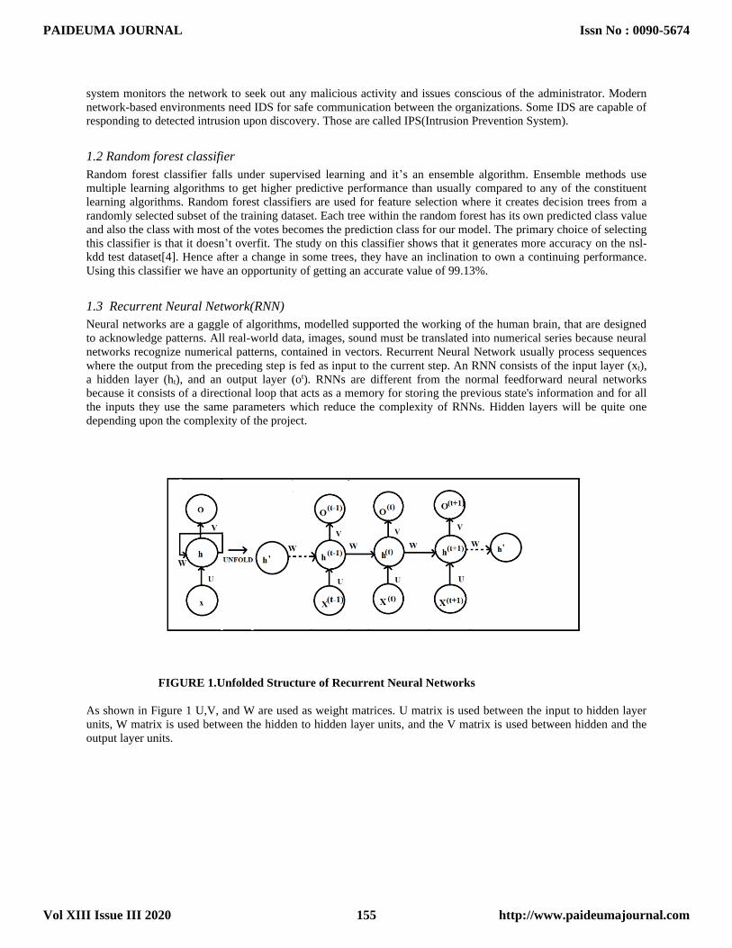
system monitors the network to seek out any malicious activity and issues conscious of the administrator. Modern

network-based environments need IDS for safe communication between the organizations. Some IDS are capable of

responding to detected intrusion upon discovery. Those are called IPS(Intrusion Prevention System).

1.2 Random forest classifier

Random forest classifier falls under supervised learning and it’s an ensemble algorithm. Ensemble methods use

multiple learning algorithms to get higher predictive performance than usually compared to any of the constituent

learning algorithms. Random forest classifiers are used for feature selection where it creates decision trees from a

randomly selected subset of the training dataset. Each tree within the random forest has its own predicted class value

and also the class with most of the votes becomes the prediction class for our model. The primary choice of selecting

this classifier is that it doesn’t overfit. The study on this classifier shows that it generates more accuracy on the nsl-

kdd test dataset[4]. Hence after a change in some trees, they have an inclination to own a continuing performance.

Using this classifier we have an opportunity of getting an accurate value of 99.13%.

1.3 Recurrent Neural Network(RNN)

Neural networks are a gaggle of algorithms, modelled supported the working of the human brain, that are designed

to acknowledge patterns. All real-world data, images, sound must be translated into numerical series because neural

networks recognize numerical patterns, contained in vectors. Recurrent Neural Network usually process sequences

where the output from the preceding step is fed as input to the current step. An RNN consists of the input layer (xt),

a hidden layer (ht), and an output layer (ot). RNNs are different from the normal feedforward neural networks

because it consists of a directional loop that acts as a memory for storing the previous state's information and for all

the inputs they use the same parameters which reduce the complexity of RNNs. Hidden layers will be quite one

depending upon the complexity of the project.

FIGURE 1.Unfolded Structure of Recurrent Neural Networks

As shown in Figure 1 U,V, and W are used as weight matrices. U matrix is used between the input to hidden layer

units, W matrix is used between the hidden to hidden layer units, and the V matrix is used between hidden and the

output layer units.

PAIDEUMA JOURNAL


Issn No : 0090-5674


1.4 Gated Recurrent Unit

Gated Recurrent Unit (GRU) came into existence to overcome the vanishing gradient hassle that is seen in the

regular RNN. GRU was build by using two gates the update and the reset gates. The update gate helps the model to

determine how much past information is needed to be passed along the future. The reset gate is mainly used to select

how much of the past information needs to be forgotten. The reset gate helps the GRU-IDS model to remove

unwanted information in the future.

FIGURE 2. Structure of GRU

Where,

xₜ = input at time step t.

hₜ = hidden layer input at time step t.

zₜ = update gate output at time step t.

rₜ = reset gate output at time step t.

PAIDEUMA JOURNAL


Issn No : 0090-5674


II. RELATED WORK

S.Revathi, A Malathi (2013)[8], done a detailed study on NSL-KDD dataset. They found out that the NSL-KDD

dataset consists of four classes of attacks and one normal class. They have used data mining techniques like J48,

Random forest, Naïve Bayes, CART and SVM to find attack classes from the normal class. The Random Forest

Classifier shows good results on the test dataset accuracy.

Bhupendra Ingre, Anamika Yadav (2015)[9], proposed an Intrusion Detection System using ANN and calculated

various performance measures like Accuracy, Detection Rate, and False Positive Rate. This model shows an

accuracy rate of 81.2% and 79.9% on the train and test NSL-KDD datasets.

AK Shrivas, AK Dewangan (2014)[10], proposed an Intrusion Detection System which is a combination of ANN

and Bayesian net classifier and uses the Gain ratio for reducing the feature vector. This model gave an accuracy of

99.42% with KDD99 and 98.07% with the NSL-KDD data set. So we are considering this and providing result

which is similar to this model.

H Chae, B jo, SH Choi, T Park (2013)[11], proposed a new feature selection method using feature average of total

and each class. They also used a feature reduction algorithm called Decision tree classifier to reduce the

dimensionality of the input vector.

C Yin, Y Zhu, J Fei, X He (2017)[12], developed an Intrusion Detection System using Recurrent neural networks.

This Intrusion Detection System is trained and tested using the benchmarked NSL-KDD dataset. This model was

then compared with the traditional machine learning classifiers like Support Vector Machines, Random Forest,

Naive Bayes, and J48. The metrics used for evaluating the RNN-IDS was the detection rate and accuracy. This

model shows an accuracy rate of 99.81% and 83.3% on the train and test NSL-KDD datasets.

SM Kasongo, Y Sun (2019)[13], proposed an Intrusion Detection System using the technique of Deep Long Short-

Term Memory(DLSTM) for storing the past information without losing it with time. This model outperforms over

the methods such as Deep Feed-forward Neural Networks, Support Vector Machines, k-Nearest Neighbors, Random

Forests and Naive Bayes. A feature selection algorithm based on information gain was used to reduce the feature

vector. To achieve better results Information gain feature selection method was used. The accuracy of this model on

the training and testing datasets was 99.51% and 86.99%.

SM Kasongo, Y Sun (2019)[14], a Deep Learning method using feed-forward deep neural networks(FFDNN)

besides a feature selection algorithm using information gain(IG) was used. In this work, the FFDNN with IG was

evaluated on the nsl-kdd intrusion detection dataset. This model FFDNN-IDS outperforms over various other

models like k-Nearest Neighbors(KNN), Naive Bayes, Support Vector Machine(SVM), Random Forest (RF) and

Decision Trees(DT). This model shows an accuracy rate of 99.37% and 86.76% on the train and test NSL-KDD

datasets.

III. DATASET DESCRIPTION

In our work to deal with the detection of intrusions we have taken the standard NSL-KDD dataset which is an

updated version of kdd cup 99. The advantages of the nsl-kdd dataset are

I. The dataset consists of distinct records so that the classifiers will not produce any biased result.

II. No overfitting of the result.

The NSL-KDD dataset is composed of 41 attributes and one categorized attribute. The training is performed on the

nsl-kdd train dataset which contains 22 attack types and testing is performed on the nsl-kdd test dataset which

contains additional 17 attack types. The attack classes present in nsl-kdd dataset are grouped into four categories

1.Denial of service(DoS): The authorized users will be blocked by intruders from using their service.

2.Probe: This attack collects information about potential vulnerabilities of the target system that can be later used to

launch attacks on that system

3.Remote to Local(R2L): Unauthorized users gain privileges as a root user by dumping the data packets to remote

systems over a network and do unauthorized activities.

4.User to Root(U2R): Intruders access the administrative privileges by entering into the network as normal users.

PAIDEUMA JOURNAL


Issn No : 0090-5674


IV. PROPOSED SYSTEM

We have developed an Intrusion Detection System using a Recurrent Neural Network with the gated recurrent units.

The recurrent neural network comprises the input unit, hidden unit, and output units. The hidden unit consists of all

mathematical computations. We are taking nsl-kdd dataset as input and it consists of the training and the testing

datasets. First the input data has to be pre-processed to remove any irrelevant data and then we applied Feature

Selection on the target data to reduce the dimensionality of the input data. Then, we fed this input data to the

Recurrent Neural Networks with GRU units to train the GRU-IDS and finally test the proposed model with the nsl-

kdd test dataset.

FIGURE 3.Proposed System

4.1 DATA PREPROCESSING

1) Conversion of Non-Numeric values to Numeric values

The GRU-IDS can accept only numeric values as input. The NSL-KDD dataset consists of 41 features out of which

38 are in numerical form and 3 are of string datatype. The non-numeric features are labelled as ‘protocol_type’,

‘service’ and ‘flag’ which are of string type to be converted into numeric form. To do this we used the Hot encoding

technique to convert the non-numeric features to numeric features.

2) Normalization

The GRU-IDS works with the input which is only in the range of 0 to 1. As the input data we get is not in the

specific range[0-1]. So here we applied a Min-max scaling technique to scale the input data in the range between 0

to 1. The below equation was applied to each input feature in the nsl-kdd dataset.

I’= ( I- minⱼ) / ( maxⱼ - minⱼ)

In the above equation, I is the unnormalized value of a particular attribute, I’ is the changed value of the attribute

which is in the normalized form and maxⱼ and minⱼ are the maximum and minimum values of the jth attribute.

PAIDEUMA JOURNAL


Issn No : 0090-5674


4.2 Feature Selection

The NSL-KDD dataset has 41 attributes and one class attribute. From those 41 attributes, some of the attributes will

not be useful in the detection of intrusion. So, we are using the random forest classifier to remove some of the

unimportant attributes of the train and test datasets that resolves the problem of overfitting and decrease the training

time of the GRU-IDS model.

4.3 Designing of the Gated Recurrent Unit

In our work, the proposed system GRU-IDS takes the nsl-kdd train dataset as a input vector (Xₜ) and multiplies it

with the weight matrix(Wz ). From the hidden layer of the previous time step, we take ht-1 as input which gives past

information and then it is also multiplied by the weight matrix (Uz). Wz*Xt and Uz*Xt were added together and

passed to the SoftMax function to get the update gate’s output(Zt) in the range between 0 to 1. This operation will be

useful to prevent the vanishing gradient problem because the model keeps track of all the past information without

any loss. In the same way, the reset gate(rt) is constructed. Now we make use of the reset and update gates in the

GRU cell as shown in Figure 2. To store the relevant information from the past we use the reset gate(rt). First, we

multiply Xt with a weight matrix Wh. Secondly, we apply Hadamard product between the reset gate rt and ht-1 and

sum the result of Hadamard product with Wh*Xt and apply tanh activation function to the obtained result and store

the result in ht’ which stores only the relevant information from the past called as current memory content. Finally

we calculate the final memory at time step t. Now we make use of the update gate(Zt) which consists of the

information to be passed at time step t. Calculate element-wise multiplication between Zt and ht’ and between 1-Zt

and ht-1 then sum up both of them and store the result in ht. The ht will tell the GRU model how much of the past

information to be useful; this will make the GRU model train perfectly without any loss of the past information

V. EVALUATION METRICS

To examine the performance of the GRU-IDS we specifically used Accuracy(AC) as a performance indicator. The

other performance measures used are Detection Rate, and False Positive Rate. The output of the GRU-IDS model is

categorized based on the following four conditions:

True Positive (TP): The number of anomaly records that are correctly classified as anomaly.

False Positive(FP): The number of normal records that are incorrectly classified as anomaly.

True Negative(TN): The number of normal records that are correctly classified as normal.

False Positive(FN): The number of anomaly records that are incorrectly classified as normal.

From the above-defined TP, FP, TN, FN metrics we can define Accuracy, Detection Rate, and False Positive Rate.

Accuracy(AC): It is the percentage of the number of records that are correctly classified out of the total number of

records.

Accuracy = (TP+TN) / (TP+TN+FP+FN)

Detection Rate(DR): It is the percentage of the number of records that are classified correctly out of the total number

of anomaly records.

Detection Rate(DR) = TP / TP+FN

False Positive Rate(FPR): It is the percentage of the number of records that are incorrectly classified out of the total

number of normal records.

False Positive Rate(FPR)= FP / FP + TN

PAIDEUMA JOURNAL


Issn No : 0090-5674


The Confusion matrix visualizes the performance of the GRU-IDS model as shown below.

Table 1. Confusion Matrix

VI. EXPERIMENTALRESULTS

The experimental results show that our proposed system GRU-IDS gives better accuracy on the test dataset

compared to various traditional machine learning classifiers as shown in Table 2. The GRU-IDS also gives more

accuracy rate compared to simple RNN and LSTM based techniques. From Table 3, we observe that our proposed

system’s accuracy varies with the number of hidden nodes present in the hidden layer of recurrent neural networks.

Table 2. Performance of the existing systems.

IDS SYSTEM Validation Accuracy Test Accuracy

SVM 99.55% 78.32%

KNN 99.42% 73.26%

NB 89.32% 75.62%

RF 99.73% 83.92%

ANN 99.49% 84.17%

RNN 97.53% 82.74%

LSTM 98.12% 85.42%

Table 3. Performance of our proposed system GRU-IDS.

Hidden Nodes Validation Accuracy Test Accuracy

40 95.15% 76.78%

80 99.42% 85.34%

120 99.13% 89.22%

160 96.18% 82.17%

200 97.35% 79.19%

PAIDEUMA JOURNAL


Issn No : 0090-5674


VII. CONCLUSION AND FUTURE WORK

This model mainly focused on Intrusion detection with a high accuracy rate using RNN and feature selection

algorithm Random forest classifier. The experimental results shows an accuracy rate of 99.13%.on the training

dataset and 89.22% on the test data. This model outperforms all the other existing Intrusion Detection Systems. In

our future research, we would like to focus on decreasing the time complexity and increasing the accuracy rate in

detecting intrusions in a network system.

VIII. REFERENCES

[1]. Sharma S, Gupta RK. Intrusion detection system: A review. International Journal of Security and

its Applications.2015;9(5):69-76.

[2]. Allen J, Christie A, Fithen W, McHugh J, Picket J. State of the practice of intrusion detection technologies.

CARNEGIE-MELLON UNIV PITTSBURGH PA SOFTWARE ENGINEERING INST; 2000 Jan.

[3].Reddy RR, Ramadevi Y, Sunitha KN. Effective discriminant function for intrusion detection using SVM.in 2016

International Conference on Advances in Computing. Communications and informatics (ICACCI) 2016 Sep

21(pp.1148-1153). IEEE.

[4].Farnaaz N, Jabbar MA.Random forest modeling for network intrusion detection system. Procedia Computer

Science.2016 Jan 1;89(1):213-7.

[5].Selvakumar B, Muneeswaran K. Firefly algorithm based feature selection for network intrusion

detection.Computers & Security. 2019 Mar 1;81:148-55.

[6].Li W, Yi P, Wu Y, Pan L, Li J.A new intrusion detection system based on KNN classification algorithm in the

wireless sensor network. Journal of Electrical and Computer Engineering 2014;2014.

[7].Sahu S, Mehtre BM. Network intrusion detection system using J48 Detection Tree. In 2015 International

Conference on Advances in Computing, Communications, and Informatics (ICACCI) 2015 Aug 10(pp. 2023-2026).

IEEE.

[8].Revathi S, Malathi A. A detailed analysis of NSL-KDD dataset using various machine learning techniques for

intrusion detection. International Journal of Engineering Research & Technology (IJERT). 2013 Dec;2(12):1848-53.

[9]In GRE B, Yadav A. Performance analysis of NSL-KDD dataset using ANN. In 2015 international conference on

signal processing and communication engineering systems 2015 Jan 2(pp. 92-96).IEEE.

[10]. Shrivas AK, Dewangan AK. An ensemble model for classification of attacks with feature selection based on

KDD99 and NSL-KDD data set. International Journal of Computer Applications.2014;99(15):8-13.

[11]. Chae HS, Jo BO, Choi SH, Park TK. Feature selection for intrusion detection using NSL-KDD.Recent

advances in computer science.2013 Nov:184-7.

[12]. Yin C, Zhu Y, Fei J, He X. A deep learning approach for intrusion detection using recurrent neural networks.

Ieee Access.2017 Oct 12;5:21954-61.

[13]. Kasongo SM, Sun Y.A Deep Long Short-Term Memory based classifier for Wireless Intrusion Detection

System. ICT Express. 2019 Aug 22.

[14]. Kasongo SM, Sun Y.A deep learning method with a filter-based feature engineering for the wireless

intrusion detection system. IEEE Access. 2019 Mar 18;7:38597-607.

PAIDEUMA JOURNAL


Issn No : 0090-5674


intrusion detection system using gated recurrent …

Documents