XV International PhD WorkshopOWD 2013, 19-22 October 2013

Influence of a Tracking Data Generation Methodin a Nonlinear Control of a Biped Robot

Adam Wojciech Łukomski, West Pomeranian University of Technology, Szczecin(29.11.2012, prof. Zbigniew Emirsajłow, West Pomeranian University of Technology, Szczecin)

Abstract

This paper presents a short discussion of the influ-ence that an incorrect choice of a tracking data gen-eration method can have during the control of abiped robot. In the analysed example a two-leggedrobot with a torso is controlled using a basic non-linear feedback method.

1 IntroductionIn this paper a basic approach to simulation andcontrol of a 3D bipedal robot is presented. A bipedis a two-legged mechanism that is supposed to bewalking in a human-like fashion, that is with atorso kept in a vertical position and by striking theground each time with a different foot in order tokeep a constant speed of movement.

In general, the robot during simulation, as seenin Fig. 1, can be considered as a hybrid system [3],with continuous states described by dynamics andkinematics of the mechanism. The discrete statesof the robot refer to the type of support phase itis experiencing - if the biped is freely moving inthe gravitational field, then it is called the flightphase, when standing on one leg it is in a single sup-port phase and can be simplified using Pfaffian con-straints into a simple serial manipulator, and whenstanding on both legs it is in a double support phaseand can be treated as a parallel manipulator. Sincethe current work does not assume neither runningnor using both legs for support, only single supportphases will be considered.

The analysis of motion in 3D is done in three ba-sic planes of motion [8], that is sagittal (side view,analysis of leg behaviour), frontal (front view, sta-bilisation of posture) and transverse (top view, nav-igation) as seen in Fig. 2.

One of the reasons for this experiment is toverify whether methods other than Zero-Moment

Figure 1: Sketch of a biped model used for com-puter simulations, all controlled joints are visible.

Point are feasible for usage in simple scenarios withonly fully-actuated phase of support. Results fromthe previous experiment [5] in actuated walking areextended with the usage of a correct torso model,full trajectory for the leg tip and inverse kinematicsthat rewrite it for individual joints [4].

2 Modelling

The robot that is used for verification of the algo-rithms is a standard Robotis Bioloid biped, whichcan be seen in Fig. 3. For this experiment a fulltorso, as seen in Fig. 4, is used in order to simulateproper mass distribution. Both arms are locked ina position slightly away from the torso. The massand inertia data has been derived using CAD mod-els of the robot and FreeCAD program.

In order to write down the kinematics of the

478

Figure 2: Main planes of motion: sagittal, frontaland transverse.

mechanism the Lie algebra elements (6D vectors),that describe the way a joint moves in the 3D space[1], are needed as

s =(ωv

)(1)

where ω is the rotational part and v is the transla-tion, and in particular in the case of pure rotations

s =(

ωz × ω

)(2)

where z is the axis of rotation for the joint.The Lie algebra elements can be either written

in 6D vector form or as an equivalent 4× 4 matrix,using a hat operator

s ∈ se(3), s =(ω v0 0

)(3)

where ω is just a skew-symmetric matrix of a vectorω. If the elements s1, s2, ... describe the rotationsin the mechanism and configuration vector q con-tains matching angles, then the placement and ori-entation of the i-th link can be described by usinga map from Lie algebra se(3) back into Lie groupSE(3), together with an initial placement of i-thlink gi(0) [6], [7]

gi(q) = es1q1es2q2 ...esiqigi(0). (4)

Due to a quite high number of joints, the dynam-ics are derived using a recursive Newton-Euler al-gorithm [2], [5]. The dynamic model in a singlesupport phase is

H(q)q + C(q, q) = Bu (5)

where H is the mass-inertia matrix, vector C com-bines the effects of centripetal, Coriolis and gravityforces, B is an input transformation matrix and u

Figure 3: Robot with torso attached, all control-lable motors shown

is a vector of inputs. This can be transformed intoa standard nonlinear control-affine form

x = f(x) + g(x)u (6)

x =(

qH−1(−C)

)+

(0

H−1Bu

)(7)

where x = ( qq ) is the state.

When the tip of the swing leg of the robottouches the ground, an instantaneous double-support phase occurs, that is an impact that onlychanges the velocity of the robot, not the con-figuration. After a velocity loss legs need to beswitched, in order to use the same kinematics equa-tions, so a simple mapping for both those actions iscreated as (

q+q+

)= I

(q−q−

)I is a function describing impacts (comes fromphysical constraints and integration of dynamicequations) and leg switching, q−,q− is the positionand velocity before, and q+,q+ after the impact.

3 Control methodFor the nonlinear system (6) it is possible to chooseinputs in a way that will linearise it from the input-output perspective. The choice of outputs is de-scribed as

y = h(x) (8)

479

Figure 4: CAD view of a torso with arms in alocked position

and after taking wi derivatives of each output yi,the input signals start to appear directly

yi = hi(x)

yi =yi

∂x= Lfhi + Lghiu = Lfhi,

yi =∂yi

∂xx = L2

fhi + LgLfhiu = L2fhi,

...,

y(wi−1)i = Lwi−1

f hi + LgLwi−2f hiu = Lwi−1

f hi,

y(wi)i = Lwi

f hi + LgLwi−1f hiu.

where Lab is a Lie derivative (directional deriva-tive) of a along b, and after dropping the indices infavor of matrix equations for all inputs and outputs

y(w) = Lwf h+ LgL

w−1f hu

u =(LgL

w−1f h

)−1 (z − Lw

f h)

broughts the outputs into the linear form

y(w) = z. (9)

For the biped the relative degree w for an outputdepending only on the angles is generally 2, andthe can be stabilised to a desired value ri using forexample

zi = k1,i(ri − yi) + k2,i(ri − yi) (10)

the parameters are chosen so that ( 0 Ik1 k2

) is a Hur-witz matrix. If the chosen outputs are simplythe controlled angles then this method will turnthe system into a chain of decoupled second de-gree linear differential equations, if underactuatedthen with an addition of nonlinear functions forthe evolution of uncontrolled variables. As longas the robot centre of pressure remains inside thefoot support region, the robot behaves like a fully-actuated mechanism.

Figure 5: Key postures for the first trackingmethod, sagittal view and COM point

Figure 6: Simulated motion for the first trackingmethod

4 Tracking

Two different methods were used in order to gen-erate tracking data for the robot. The first one isbased on using 2-3 key postures, stored in memoryas full configuration states of the robot, betweenwhich a control system switches during motion.Sample configurations have been captured from hu-man motion using Kinect sensor, see Fig. 5. Speedsfor each posture during the step must be set man-ually by tuning ki,j parameters. A sample simula-tion can be seen in Fig. 14. Since this method uses arather long-distance goal for feedback linearisation,the input signals are expected to be quite high, aswell as initial angular accelerations. This can beseen in Fig. 7 and 8. Nevertheless the overall mo-tion is smooth and acceptable.

Second method involves declaring a starting g0and ending gf positions of feet, both with corre-sponding velocities V 1

0 ,V 12 , and calculating a curve

480

Figure 7: Input signals for the first tracking method

Figure 8: Accelerations for the first trackingmethod

yr in 3D space using de Casteljau algorithm [?],[4]

g1 = g0eV 10 , g2 = gfe

−V 12

V 11 = log(g−1

1 g2)

V 20 = log(e(1−t)V 1

0 etV11 )

V 21 = log(e(1−t)V 1

1 etV12 )

V 30 = log(e(1−t)V 2

0 etV21 )

yr(t) = g0etV 1

0 etV20 etV

30

As the next step, the curve in 3D space needs to betranslated through velocity

xr = log(yr(t−)−1yr(t+))

(where t−, t+ are time moments close to eachother, to ease implementation) into joint velocitiesusing differential inverse kinematics

r = J†(q)xr + (I − J†(q)J(q))qs

where qs is a modification taking into accountphysical limitations of the mechanism [?]

qs = gradψ

ψ(q) = − 12n

n∑i=1

(qi − qim

qimax − qimin

)2

where qim, qimax, qimin - mid-range, maximal andminimal limits for the joints. In the case of an ac-tual robot they are calculated with an aid of theoperator, where a special script does

Figure 9: Simulated motion for the second trackingmethod

• ask the operator to aid the robot in making 10steps

• checks the average data for boundaries, limita-tions

• extends them to fit every occuring data point,+10%

which, despite being just an average of what humanoperator wishes the robot’s movement to be, wasshown to be enough to ensure correct limitationsfor normal motion.

The initial simulation that uses two of thekey posture, together with basic upright veloci-ties (more information is available in [4], but onlysimulations of this particular case and planar casewhere presented, without verification) can be seenin Fig. 9. Inputs and acceleration can be seenin Fig. 10 and 11, and it is clear that motion ismore smooth due to a lack of discontinuity whenit comes to tracking data, that occurs between keypostures. Despite the initial high input signal themotion should be feasible for verification on theavailable hardware.

5 ResultsAfter a computer simulation using dynamic modelthe data regarding configuration is transferred tothe robot for verification. Previous attempts at dif-ferent kinds of control, kinematic and dynamic, ofthe robot has shown, that a simple kinematic loop,where at each time step only positions and veloci-ties are sent and the robots’ servomechanisms workin their inner PID loops, is sufficiently precise forbasic verification of control algorithm’s results.

481

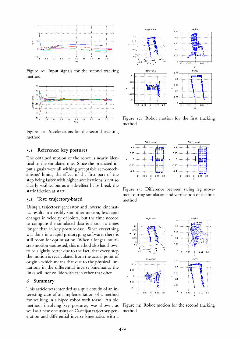
Figure 10: Input signals for the second trackingmethod

Figure 11: Accelerations for the second trackingmethod

5.1 Reference: key posturesThe obtained motion of the robot is nearly iden-tical to the simulated one. Since the predicted in-put signals were all withing acceptable servomech-anisms’ limits, the effect of the first part of thestep being faster with higher accelerations is not soclearly visible, but as a side-effect helps break thestatic friction at start.

5.2 Test: trajectory-basedUsing a trajectory generator and inverse kinemat-ics results in a visibly smoother motion, less rapidchanges in velocity of joints, but the time neededto compute the simulated data is about 10 timeslonger than in key posture case. Since everythingwas done in a rapid prototyping software, there isstill room for optimisation. When a longer, multi-step motion was tested, this method also has shownto be slightly better due to the fact, that every stepthe motion is recalculated from the actual point oforigin - which means that due to the physical lim-itations in the differential inverse kinematics thelinks will not collide with each other that often.

6 SummaryThis article was intended as a quick study of an in-teresting case of an implementation of a methodfor walking in a biped robot with torso. An oldmethod, involving key postures, was shown, aswell as a new one using de Casteljau trajectory gen-eration and differential inverse kinematics with a

Figure 12: Robot motion for the first trackingmethod

Figure 13: Difference between swing leg move-ment during simulation and verification of the firstmethod

Figure 14: Robot motion for the second trackingmethod

482

Figure 15: Difference between swing leg movementduring simulation and verification of the secondmethod

slight modification for taking into considerationphysical limitations. Both were again verified ona bipedal robot, with torso included for addedweight.

The torque-based verification was discarded andnormal kinematic-following approach was used,with acceptable results. Further study into nav-igation in transverse plane should show whetherthe assumptions made in this preliminary study arecorrect.

References[1] Roy Featherstone. A beginner’s guide to 6-d

vectors (part 2)[tutorial]. Robotics & Automa-tion Magazine, IEEE, 17(4):88–99, 2010.

[2] Roy Featherstone and David Orin. Robot dy-namics: equations and algorithms. In Roboticsand Automation, 2000. Proceedings. ICRA’00.IEEE International Conference on, volume 1,pages 826–834, 2000.

[3] Jessy W. Grizzle, Christine Chevallereau,Aaron D. Ames, and Ryan W. Sinnet. 3dbipedal robotic walking: models, feedback con-trol, and open problems. In IFAC Symposiumon Nonlinear Control Systems, 2010.

[4] Adam Wojciech Lukomski. Method for gen-erating a biped swing leg trajectory duringwalking. In International Interdisciplinary PhDWorkshop, Brno, Czech Republic, 2013.

[5] Adam Wojciech Lukomski. Simple experimentof an actuated walking in a biped robot. In 9thInternational Workshop on Robot Motion andControl, 2013.

[6] J. M. Selig. Geometric fundamentals of robotics.Springer Science+ Business Media Incorpo-rated, 2005.

[7] J. M. Selig and Yuanqing Wu. Interpolatedrigid-body motions and robotics. In Intelli-

gent Robots and Systems, 2006 IEEE/RSJ Inter-national Conference on, pages 1086–1091, 2006.

[8] Aydin Tözeren. Human body dynamics: classi-cal mechanics and human movement. SpringerVerlag, 2000.

Author

Adam Wojciech ŁukomskiWest Pomeranian University ofTechnology, Faculty of ElectricalEngineering, Department of Con-trol and Measurementul. 26 Kwietnia 1071-126 Szczecinemail: lukomski@zut.edu.pl

483