inﬂuence of nuclear substructure on gene regulation and...

Influence of Nuclear Substructure on Gene Regulation and Expression

Samuel Isaacson

in collaboration with:Carolyn Larabell (UCSF/LBL),

David McQueen (NYU), Charles Peskin (NYU)

Friday, July 13, 12

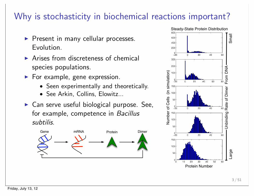
Why is stochasticity in biochemical reactions important?

! Present in many cellular processes.Evolution.

! Arises from discreteness of chemicalspecies populations.

! For example, gene expression.• Seen experimentally and theoretically.• See Arkin, Collins, Elowitz...

! Can serve useful biological purpose. See,for example, competence in Bacillus

subtilis.Gene mRNA Protein Dimer

Num

ber o

f Cel

ls (

in s

imul

atio

n)Protein Number

Steady7State Protein Distribution

Unb

indi

ng R

ate

of D

imer

Fro

m D

NA

Smal

lLa

rge

3 / 51

Friday, July 13, 12

What does the inside of a eukaryotic cell look like?! This is an X-ray CT image of mouse olfactory epithelial cell.! In this example a mouse cell is imaged inside a glass capillary.! Pixel intensity is proportional to density of material in pixel.

4 / 51

Mouse OlfactoryEpithelial Cell

Friday, July 13, 12

What does a nucleus look like in these reconstructions?

5 / 51(Nucleus of Preceding Cell)Friday, July 13, 12

How does subcellular structure influence the dynamics ofbiochemical processes within cells?

! We are exploring this question by studying the e!ect ofthree-dimensional subcellular structure on gene regulation andexpression.

6 / 51

Friday, July 13, 12



6 / 51



! The following processes are influenced by the spatial organizationof cellular substructure:

• Gene Regulation: proteins searching for a DNA binding site withinthe nucleus.

• mRNA export: mRNPs searching for nuclear pores and thentranslocating out of nucleus.

• Protein import: movement of cytosolic proteins to nuclear poresand translocation into the nucleus.

6 / 51Friday, July 13, 12



6 / 51







6 / 51







What is the influence of volume exclusion due to chromatin on

the time required for regulatory proteins to find DNA binding

sites?

6 / 51Friday, July 13, 12

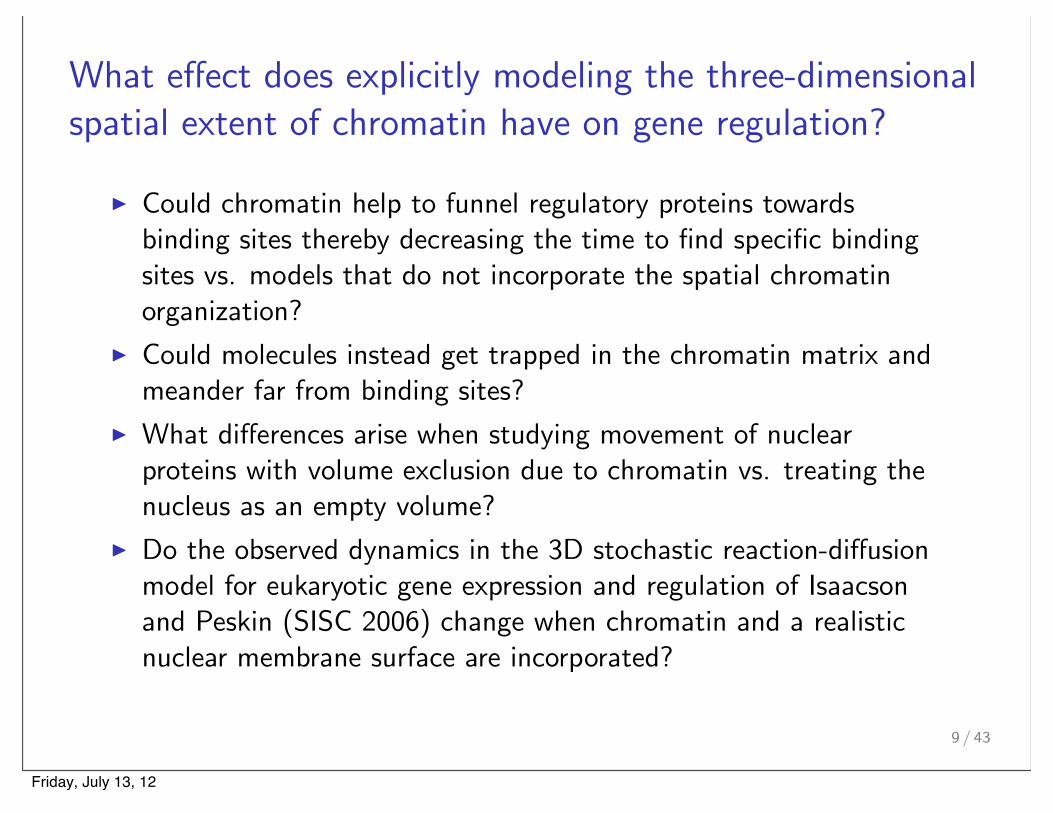
What e!ect does explicitly modeling the three-dimensionalspatial extent of chromatin have on gene regulation?

! Could chromatin help to funnel regulatory proteins towardsbinding sites thereby decreasing the time to find specific bindingsites vs. models that do not incorporate the spatial chromatinorganization?

! Could molecules instead get trapped in the chromatin matrix andmeander far from binding sites?

! What di!erences arise when studying movement of nuclearproteins with volume exclusion due to chromatin vs. treating thenucleus as an empty volume?

! Do the observed dynamics in the 3D stochastic reaction-di!usionmodel for eukaryotic gene expression and regulation of Isaacsonand Peskin (SISC 2006) change when chromatin and a realisticnuclear membrane surface are incorporated?

9 / 43

Friday, July 13, 12

•How can we construct a mathematical model of the time to find a binding site using high-resolution DAPI fluorescence data?

•What happens if we study this question with more quantitative X-ray CT data?

•What properties of nuclear substructure might contribute to our observed results?

Outline:

Friday, July 13, 12

Mouse myoblast cell nucleus(Structured Illumination Microscopy of Schermelleh et al. Science 2008)

Friday, July 13, 12

How to model volume exclusion due to chromatin?

! We assume that regions of higher DAPI fluorescence intensity aremore repulsive (harder to di!use into).

! Volume exclusion due to chromatin is modeled as a repulsivepotential, !i, experienced by di!using regulatory proteins.

! We have considered several functional relationships between thepotential !i and the DAPI fluorescence intensity, Ii.

! For the remainder of the talk we choose a linear relationship,

!i = !maxIi,

Movie of the potential as we move through the cell along z axis.

15 / 43

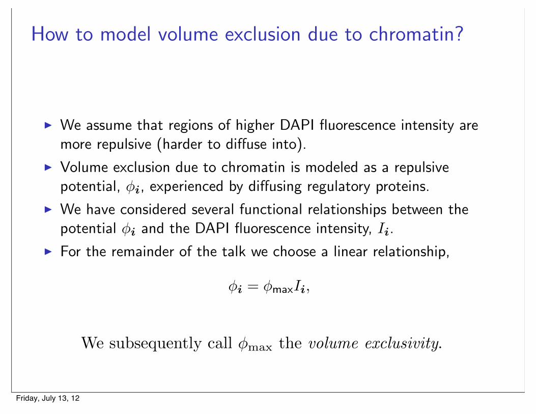
How to model volume exclusion due to chromatin?

! We assume that regions of higher DAPI fluorescence intensity aremore repulsive (harder to di!use into).

! Volume exclusion due to chromatin is modeled as a repulsivepotential, !i, experienced by di!using regulatory proteins.

! We have considered several functional relationships between thepotential !i and the DAPI fluorescence intensity, Ii.

! For the remainder of the talk we choose a linear relationship,

!i = !maxIi,

Movie of the potential as we move through the cell along z axis.

15 / 43

We subsequently call �max

the volume exclusivity.

Friday, July 13, 12

How do we model the search process of a protein for aDNA binding site?

For now, we consider a spatially-continuous model:

! We assume the protein di!uses in the repulsive potential, !(x).

! Motion of the protein within the nucleus is then governed by aFokker-Planck partial di!erential equation.

! The binding site is modeled as a sphere of radius rbind about thethe point, xbind.

! Let D be the di!usion constant of the protein.

! Denote by "(x, t) the probability density the protein has not yetfound the binding site, and is located at x, at time t.

16 / 43Friday, July 13, 12

How do we model the search process of a protein for aDNA binding site? (2)

! Within the nucleus the Fokker-Planck equation describing theprotein’s motion is:

!"

!t(x, t) = D! ·

!

!"(x, t) +1

kBT"(x, t)!#(x, t)

"

! An absorbing boundary condition is used to model binding:

"(x, t) = 0, |x" xbind| = rbind

! At the nuclear membrane a no-flux boundary condition preventsthe protein from di!using out of the nucleus:

"D#

!"(x, t)+1

kBT"(x, t)!#(x, t)

$

·!(x) = 0, #x $ membrane,

where !(x) denotes the normal to the nuclear membrane at x.

17 / 43

Friday, July 13, 12



!"

!t(x, t) = D! ·

!

!"(x, t) +1

kBT"(x, t)!#(x, t)

"




"D#

!"(x, t)+1

kBT"(x, t)!#(x, t)

$


where !(x) denotes the normal to the nuclear membrane at x.

17 / 43



!"

!t(x, t) = D! ·

!

!"(x, t) +1

kBT"(x, t)!#(x, t)

"




"D#

!"(x, t)+1

kBT"(x, t)!#(x, t)

$


where !(x) denotes the normal to the nuclear membrane at x.! However, since the underlying imaging data and potential

are defined on a lattice, we use a discrete approximation to

this equation.17 / 43

Friday, July 13, 12

What is the spatially discrete model?

! We use a discretization of the Fokker-Planck equation that hasthe form of a reaction-di!usion master equation (RDME).

! To account for the nuclear membrane we use an extension of theembedded boundary method of Isaacson et al., SISC (2006).

! Discretization takes into account the intersection of the nuclearmembrane with the natural mesh given by the imaging voxels.

! Movie of a fly-through of the cell showing cut planesperpendicular to the y-axis. Both the Cartesian mesh and thenuclear membrane are shown.

18 / 43

Friday, July 13, 12

How do we discretize the Fokker-Planck equation?Consider the one-dimensional Fokker-Planck equation

!"

!t(x, t) +

!F

!x(x, t) = 0,

where the flux, F (x, t), is given by

F (x, t) = !D

!

!"

!x(x, t) +

"(x, t)

kBT

!#

!x(x)

"

.

20 / 43

Friday, July 13, 12


!"

!t(x, t) +

!F

!x(x, t) = 0,


F (x, t) = !D

!

!"

!x(x, t) +

"(x, t)

kBT

!#

!x(x)

"

.

20 / 43


!"

!t(x, t) +

!F

!x(x, t) = 0,


F (x, t) = !D

!

!"

!x(x, t) +

"(x, t)

kBT

!#

!x(x)

"

.

Let

! pi(t) " "(ih, t), the probability density the regulatory protein isat location ih at time t.

! Fi(t) " F (ih, t) and #i " #(ih).

20 / 43Friday, July 13, 12


!"

!t(x, t) +

!F

!x(x, t) = 0,


F (x, t) = !D

!

!"

!x(x, t) +

"(x, t)

kBT

!#

!x(x)

"

.

20 / 43


!"

!t(x, t) +

!F

!x(x, t) = 0,


F (x, t) = !D

!

!"

!x(x, t) +

"(x, t)

kBT

!#

!x(x)

"

.

Let


! Fi(t) " F (ih, t) and #i " #(ih).

20 / 43


!"

!t(x, t) +

!F

!x(x, t) = 0,


F (x, t) = !D

!

!"

!x(x, t) +

"(x, t)

kBT

!#

!x(x)

"

.

Let


! Fi(t) " F (ih, t) and #i " #(ih).

We look for a discretization of the form

dpidt

(t) +1

h

#

Fi+1/2 ! Fi!1/2

$

= 0.

20 / 43

Friday, July 13, 12

How do we discretize the Fokker-Planck equation? (2)

We also assume that

Fi+1/2 = !("i+1 ! "i) pi ! #("i+1 ! "i) pi+1.

where ! and # are functions to be determined. Notice

Fi+1/2 = [!("i+1 ! "i)! #("i+1 ! "i)]

!

pi+1 + pi2

"

! [!("i+1 ! "i) + #("i+1 ! "i)]

!

pi+1 ! pi2

"

.

We choose the second term to approximate the di!usive componentof the flux, so that the standard three-point discrete Laplacian isrecovered:

!("i+1 ! "i) + #("i+1 ! "i) =2D

h.

21 / 43

Friday, July 13, 12

How we can use detailed balance to determine ! and "?

Following Wang et al. (JTB 2003), in thermodynamic equilibrium weexpect the probability density the molecule is at position x to beproportional to the Boltzmann distribution.

!eq(x) ! e!!(x)/kBT .

We therefore require that

peqi+1 = peqi e(!i!!i+1)/kBT ,

where peqi = limt"# pi(t). Moreover, at thermodynamic equilibriumdetailed balance requires that

Fi+1/2 = 0.

Combining these last two equations we obtain a second equation for "and #.

22 / 43

Friday, July 13, 12

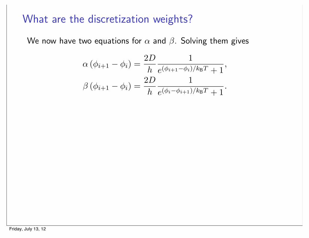
What are the discretization weights?

We now have two equations for ! and ". Solving them gives

! (#i+1 ! #i) =2D

h

1

e(!i+1!!i)/kBT + 1,

" (#i+1 ! #i) =2D

h

1

e(!i!!i+1)/kBT + 1.

! These two functions then determine the flux, Fi+1/2.

! The overall discretization is second order in space.! To discretize the three-dimensional Fokker-Planck equation in

complex geometries! We extend the one-dimensional discretization to three-dimensions.! We use the expressions for the three-dimensional flux from this

discretization in the Cartesian grid embedded boundary method ofIsaacson et al. (SISC 2006).

23 / 43

Friday, July 13, 12



! (#i+1 ! #i) =2D

h

1

e(!i+1!!i)/kBT + 1,

" (#i+1 ! #i) =2D

h

1

e(!i!!i+1)/kBT + 1.





23 / 43



! (#i+1 ! #i) =2D

h

1

e(!i+1!!i)/kBT + 1,

" (#i+1 ! #i) =2D

h

1

e(!i!!i+1)/kBT + 1.





23 / 43Friday, July 13, 12

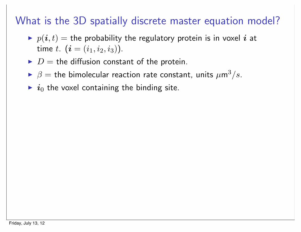
What is the 3D spatially discrete master equation model?

! p(i, t) = the probability the regulatory protein is in voxel i attime t. (i = (i1, i2, i3)).

! D = the di!usion constant of the protein.

! ! = the bimolecular reaction rate constant, units µm3/s.

! i0 the voxel containing the binding site.

24 / 43Friday, July 13, 12






24 / 43






Then

dp

dt(i, t) = D

!

j

[ki,jp(j, t)! kj,ip(i, t)]!!

Vi0

"i,i0p(i0, t),

where"

#

$

ki,j =2DAi,j

hdVj

1exp((!i!!j)/kBT)+1

, i a neighbor of j,

0, else.

24 / 43

Friday, July 13, 12

How to solve the system of di!erential-di!erenceequations?

! We could solve the system of ODEs numerically.! For the voxel mesh determined by the image planes we get a

480x480x37 system of ODEs.! This approach will be impractical when we have more than a few

di!using proteins.! Also, if the binding site location is itself a random variable, then

these equations contain a random coe"cient.! Instead, we create realizations of the stochastic process described

by the ODEs, that of a molecule undergoing a continuous timerandom walk on the voxel lattice in the potential, !i.

! We can exactly simulate this process by the Gillespie method.! In the simulations, the protein hops from voxel i to j with

probability per unit time kj,i.! When entering a voxel, i0, containing a binding site, the protein

can bind with probability per unit time "/Vi0 .

25 / 43

Friday, July 13, 12










25 / 43










25 / 43Friday, July 13, 12

What does a typical protein search process for a DNA binding site look like?In our stochastic reaction-diffusion model we find:

Friday, July 13, 12

How does volume exclusion influence the time needed tofind a specific binding site?

Initial Position

Binding Site

9 / 51

Friday, July 13, 12

How does volume exclusion influence the time needed tofind a specific binding site?

For a di!usion constant of 10 µm2/s, and the initial and binding sitepositions of the previous slide:

t (seconds)

Prob[T

>t]

!max = 0!max = 1!max = 5!max = 40!max = 80

0 200 400 600 800 1000

10!2

10!1

100

!max (kBT )

medianbindingtime(seconds)

0 20 40 60 8090

100

110

120

130

140

See Isaacson, McQueen, and Peskin, PNAS (2011).

10 / 51

Friday, July 13, 12

Can we estimate the binding time distribution?The preceding distributions appear to be well-approximated by anexponential distribution, i.e.

Prob [T > t] ! 1" e!D!t.

We can estimate ! using the numerically calculated medians from ourMonte Carlo simulations. For an exponential distribution

Tmed =ln(2)

D!.

We have investigated several other ways to estimate the observedbinding rate, D!:

! Smoluchowski di!usion limited reaction rate arguments.

! Eigenvalues of the transition rate matrix for the master equation.

! Perturbation theory.30 / 43

Friday, July 13, 12


Prob [T > t] ! 1" e!D!t.


Tmed =ln(2)

D!.






Prob [T > t] ! 1" e!D!t.


Tmed =ln(2)

D!.





Friday, July 13, 12

Can we estimate the binding time distribution?(2)Denote by V the volume of the nucleus.

1. Standard di!usion limited reaction-rate theory

! !4"rbV

.

2. A lattice di!usion limited reaction-rate theory gives

1

!!

16

(2")3V

hxhyhz

!!! !/2

0

d#d$d%"

sin(")hx

#2+

"

sin(#)hy

#2+"

sin($)hz

#2 .

3. Denote by p(t) the vector with components pi(t) = p(i, t). Then

dp

dt(t) = Lp(t),

where L denotes the transition matrix. We can estimate thebinding rate by the smallest eigenvalue of L.

31 / 43

Friday, July 13, 12

Can we estimate the binding time distribution?(3)

For example, when !max = 0 we find the following estimates for therate D":

Monte Carlo DLR Latt. DLR Trans. Mat. Eval.

.005038 ± .000039 .0094 to .0326 .00524 .0050

We have more recently derived estimates for the smallest eigenvalueof L through perturbation theory arguments.

32 / 43

Friday, July 13, 12

How could we do better?

• This data only shows the densest regions of DNA/chromatin.

• To get a better feel for the amount of nuclear DNA we are collaborating with the Larabell Lab to use their X-ray CT imaging data.

• The new X-ray data gives linear absorption coefficients within each voxel that are proportional to the amount of organic material in that voxel.

Friday, July 13, 12

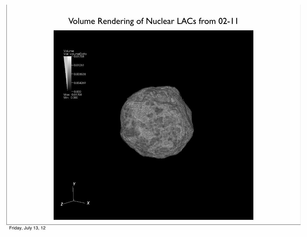
Volume Rendering of Nuclear LACs from 02-11

Friday, July 13, 12

Normalized Histogram of Normalized Nuclear LACs.Markers denote every tenth percentile.

data02-11 data05-14

data05-15 data09-03

Friday, July 13, 12

How do we model the search for a binding site using this new data?

• Still model volume exclusion as a repulsive potential felt by the diffusing protein.

• The potential of each voxel is proportional to the normalized measured LAC of that voxel.

•Again, when the volume exclusivity is zero the protein simply diffuses (the chromatin is not felt by the protein).

•As this parameter is increased the maximum strength of the potential increases, and it becomes substantially more difficult for the protein to enter regions with large LACs.

•We will subsequently use SIM to refer to the structured illumination data and X-ray for the new X-ray CT data.

Friday, July 13, 12

Example simulation with new X-ray CT imaging data:

Friday, July 13, 12

How does binding site position influence the time needed to find a specific binding site?

• Assume the protein initiates its search from a specific pore.

‣ For the SIM data, in each simulation we sample the protein’s initial position from a uniform distribution of all possible pore locations.

‣ For the X-ray CT data, we sample the position randomly from voxels that are on the boundary of the nucleus.

•We restrict the binding site position to subregions of the nucleus with specified intensity/LAC levels.

‣Regions of very high intensity/LAC may correspond to heterochromatin.

‣Regions of low intensity/LAC to euchromatin.

Friday, July 13, 12

−10 0 10 20 30 40 50 60 70 80 9020

40

60

80

100

120

140

160

180

volume exclusivity

med

ian

bind

ing

time

(sec

onds

)

20 to 30 − SIM

20 to 30 − 09 Xray

20 to 30 − 02 Xray

20 to 30 − 05−14−nuc1 Xray

20 to 30 − 05−14−nuc2 Xray

20 to 30 − 05−15 Xray

• Binding site is a randomly chosen voxel in the 20th to 30th percentile of intensity values for each simulation.

• Initial position is chosen randomly from all pores for the SIM data, and randomly from all voxels on the nuclear membrane in the Xray data.

Median Binding Times when Binding Sites are Placed in the 20th to 30th percentile of intensity values.

Friday, July 13, 12

Speedup in fastest median binding time vs. no volume exclusion case.(For binding sites in the 20th to 30th percentile of nuclear voxel intensities.)

NucleiVolume Exclusivity of minimum binding time

(KbT)

Percent speedup vs. no volume exclusion

SIM data

Xray 09

Xray 02

Xray 05-14

Xray 05-14 Nucleus 2

Xray 05-15

40 32.69

10 31.09

10 33.93

10 25.22

10 23.83

10 28.61

Friday, July 13, 12

What do the binding time distributions look like in this case?

0 200 400 600 800 100010−6

10−5

10−4

10−3

10−2

10−1

100

t (seconds)

P[T

< t]

09 − Xray survival time distributions, 20 to 30 case

0151040

How does binding site position influence the time neededto find a specific binding site?

For a di!usion constant of 10 µm2/s.

Binding site sampled fromvoxels with intensities betweenthe 20th and 30th percentiles

of intensity values.

Binding site sampled fromvoxels with intensities betweenthe 20th and 30th percentiles

of intensity values.

t (seconds)

Prob[T

>t]

!max = 0!max = 1!max = 5!max = 40!max = 80

0 500 1000 1500 2000

10!2

10!1

100

!max (kBT )

medianbindingtime(seconds) 20 to 30

40 to 5070 to 8020 to 30 (S)

0 20 40 60 80100

150

200

250

300

350

400

450

34 / 43

SIM survival time distributions, 20 to 30 case

Here

• P[T<t] = probability binding time, T, is less than t.

• Also, note that each legend gives the volume exclusivity for a given curve.

Friday, July 13, 12

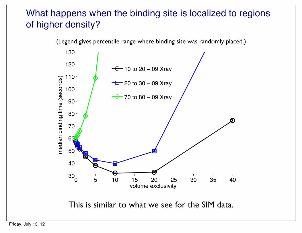
What happens when the binding site is localized to regions of higher density?

(Legend gives percentile range where binding site was randomly placed.)

0 5 10 15 20 25 30 35 4030

40

50

60

70

80

90

100

110

120

130

volume exclusivity

med

ian

bind

ing

time

(sec

onds

)

10 to 20 − 09 Xray

20 to 30 − 09 Xray

70 to 80 − 09 Xray

This is similar to what we see for the SIM data.

Friday, July 13, 12

What “fractal dimension” of euchromatin gives the most consistent binding times to our potential model?

• Based on a threshold LAC, we remove voxels above this LAC from the free space in the nucleus. (i.e. the protein is not allowed to diffuse into them).

‣ We then calculate the box-counting / fractal dimension of the remaining voxels (i.e. the “free space” / euchromatin).

• We set the volume exclusivity to zero so that in the “free space” the protein simply diffuses (i.e. no longer feels the varying density of chromatin).

• Binding sites are still chosen randomly from the subset of free space voxels that are also within the 20th to 30th percentile of intensity values from all nuclear voxels.

• We compare the minimum time to find the binding site over all volume exclusivities vs. the time for a subset of nuclear voxels.

Friday, July 13, 12

What is the box counting dimension / fractal dimension?

•We want to understand / measure how an object fills space.

• For example, consider the Hilbert Curve, a space-filling curve:

The limiting curve is one-

dimensional, but touches every

point in the box. It fills space like a

2D object.

(From Wikipedia)

Friday, July 13, 12

What is the box counting dimension / fractal dimension?

From Wikipedia

• The box counting dimension gives a measure of how an object fills the

underlying space.

• It is given by covering the object with N boxes of size h

• We then count how many, M(h), of the boxes contain a piece of the object.

• It is assumed that as h ! 0, M(h) ⇠ h�d, for some box counting dimen-

sion, d.

d = lim

h!0

log(M(h))

log(1/h)

Friday, July 13, 12

What is the Predicted Fractal Dimension of “Free Space” vs Threshold LAC Value

(slope equals the finest level box counting / fractal dimension)

data02-11

0

1

2

3

slope

0 1normalizedabsorptioncoefficient

data05-14

0

1

2

3

slope


data05-15

0

1

2

3

slope


data09-03

0

1

2

3

slope


data02-11

Distribution of Nuclear LACs

Fractal Dimension vs

Threshold LAC

data05-14 data05-15 data09-03

For all four nuclei we see that the effective box counting dimension of the voxels at or before the first “peak” in the histogram is between

two and three.

Friday, July 13, 12

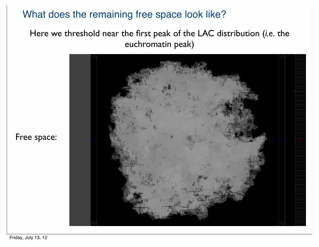
What does the remaining free space look like?

Here we threshold near the first peak of the LAC distribution (i.e. the euchromatin peak)

Free space:

Friday, July 13, 12

How are the threshold level, dimension of free space, and predicted binding time related?

Thresholded Cell / Level

Percent of intensity values at or before the

threshold value.

Finest Level Box Counting Dimension (i.e. estimated fractal

dimension)

Percent difference of median times with thresholding from

minimum median time without thresholding.

Cell 09, Level 24

Cell 09, Level 27

Cell 09, Level 30

Cell 02, Level 27

Cell 02, Level 30

27.21 2.49 -6.45

37.02 2.64 -21.17

45.22 2.74 -22.14

28.93 2.43 2.40

37.32 2.60 -13.12

Friday, July 13, 12

Summary

• Volume exclusion due to chromatin may help speed-up the time required for regulatory proteins to find specific DNA binding sites. ‣ For regions of low chromatin density (low fluorescence), weak

to moderate volume exclusivity gives the fastest times. ‣ For regions of sufficiently high density, very little or no speed-

up is seen in comparison to a model without volume exclusion. • Fastest binding times in potential model are similar to those

where we threshold near the euchromatin peak.‣ At this threshold level, the “free space” in the nucleus has a

box counting dimension of ~2.4-2.5

Friday, July 13, 12

Acknowledgements

• Collaborators: ‣ Carolyn Larabell (UCSF/LBL), X-ray CT data.‣ David McQueen and Charles Peskin, Courant Institute, NYU,

modeling and data analysis.• Ravi Iyengar and SBCNY for support and helpful discussions.• NSF and NIH for support.

Thank you for coming and inviting me!

Friday, July 13, 12

inﬂuence of nuclear substructure on gene regulation and...

Documents