invariant manifolds for stochastic partial differential · invariant manifolds for stochastic...
TRANSCRIPT
INVARIANT MANIFOLDS FOR STOCHASTIC PARTIAL DIFFERENTIALEQUATIONS
JINQIAO DUAN, KENING LU, AND BJORN SCHMALFUSS
ABSTRACT. Invariant manifolds provide the geometric structures for describing and un-derstanding dynamics of nonlinear systems. The theory of invariant manifolds for bothfinite and infinite dimensional autonomous deterministic systems, and for stochastic ordi-nary differential equations is relatively mature. In this paper, we present a unified theoryof invariant manifolds for infinite dimensional random dynamical systems generated bystochastic partial differential equations. We first introduce a random graph transform anda fixed point theorem for non-autonomous systems. Then we show the existence of gener-alized fixed points which give the desired invariant manifolds.
1. INTRODUCTION
Invariant manifolds are essential for describing and understanding dynamical behavior ofnonlinear and random systems. Stable, unstable and center manifolds have been widelyused in the investigation of infinite dimensional deterministic dynamical systems. In thispaper, we are concerned with invariant manifolds for stochastic partial differential equa-tions.
The theory of invariant manifolds for deterministic dynamical systems has a long and richhistory. It was first studied by Hadamard [9], then, by Liapunov [12] and Perron [16] usinga different approach. Hadamard’s graph transform method is a geometric approach, whileLiapunov-Perron method is analytic in nature. Since then, there is an extensive literature onthe stable, unstable, center, center-stable, and center-unstable manifolds for both finite andinfinite dimensional deterministic autonomous dynamical systems (see Babin and Vishik[2] or Bates et al. [3] and the references therein). The theory of invariant manifolds for non-autonomous abstract semilinear parabolic equations may be found in Henry [10]. Invariantmanifolds with invariant foliations for more general infinite dimensional non-autonomousdynamical systems was studied in Chow et al.[6]. Center manifolds for infinite dimensionalnon-autonomous dynamical systems was considered in Chicone and Latushkin [5].
Recently, there are some works on invariant manifolds for stochastic/random ordinary dif-ferential equations by Wanner [24], Arnold [1], Mohammed and Scheutzow [14], andSchmalfuß [19]. Wanner’s method is based on the Banach fixed point theorem on someBanach space containing functions with particular exponential growth conditions, which isessentially the Liapunov-Perron approach. A similar technique has been used by Arnold.In contrast to this method, Mohammed and Scheutzow have applied a classical technique
Date: December 10, 2001.1991 Mathematics Subject Classification. Primary: 60H15; Secondary: 37H05, 37L55, 37L25, 37D10.Key words and phrases. Invariant manifolds, cocycles, non-autonomous dynamical systems, stochastic partial
differential equations, generalized fixed points.
1
2 JINQIAO DUAN, KENING LU, AND BJORN SCHMALFUSS
due to Ruelle [17] to stochastic differential equations driven by semimartingals. In Cara-ballo et al. [22] an invariant manifold for a stochastic reaction diffusion equation of pitch-fork type has been considered. This manifold connects different stationary solutions of thestochastic differential equation. In Koksch and Siegmund [11] the pullback convergencehas been used to construct an inertial manifold for non-autonomous dynamical systems.
In this paper, we will prove the existence of an invariant manifold for a nonlinear stochasticevolution equation with a multiplicative white noise:
���������� ���� ����������
(1)
where � is a generator of a ��� -semigroup satisfying a exponential dichotomy condition,�� ����is a Lipschitz continuous operator with
�� ���� � � , and����
is the noise. The preciseconditions on them will be given in the next section. Some physical systems or fluid sys-tems with noisy perturbations proportional to the state of the system may be modeled bythis equation.
In order to show the existence of an invariant manifold, we will first show this stochasticevolution equation generates a random dynamical system by using a standard technique totransform this equation into a conjugated random evolution equation without a white noisebut with random coefficients. Then, we will prove the existence of an invariant manifoldfor the conjugated random evolution equation, and finally we will transform the resultsback to the original stochastic evolution equation.
Our method showing the existence of an invariant manifold is different from the methodsmentioned above, which is an extension of the result by Schmalfuß [18]. We will introducea random graph transform. This graph transform defines a random dynamical system onthe space of appropriate graphs. One ingredient of a random dynamical system is a cocy-cle (see the next section). An invariant graph of this graph transform is a generalized fixedpoint for cocycles. A generalized fixed point defines an entire trajectory for the cocycle.Applying this fixed point theorem to the graph transform dynamical system we can findunder a gap condition a fixed point contained in the set of Lipschitz continuous graphswhich represent the invariant manifold.
The main assumption is the gap condition formulated by a linear two-dimensional randomequation. This equation allows us to calculate a priori estimate for the fixed point theorem.We note that this linear random differential equation has a nontrivial invariant manifold ifand only if the gap condition is satisfied. Hence, our results are optimal in this sense.
We believe that our technique can be applied to other cases that are treated in Bates et al.[3].
We also note that we do not need to use the semigroup given by the skew product flow.
In Section 2, we recall some basic concepts for random dynamical systems and show thatthe stochastic partial differential equation (1) generates a random dynamical system. Weintroduce a random graph transform in Section 3. A generalized fixed point theorem ispresented in Section 4. Finally, we present the main theorem on invariant manifolds inSection 5.

INVARIANT MANIFOLDS FOR STOCHASTIC PARTIAL DIFFERENTIAL EQUATIONS 3
2. RANDOM DYNAMICAL SYSTEMS
We recall some basic concepts in random dynamical systems. Let ���������� �
be a probabil-ity space. A flow � of mappings ���� ����� is defined on the sample space
�such that
������� ������� � � �����! � �"�$#&%'���)( � �"�$#+*,�)((2)
for�.-�� �+/10 � . This flow is supposed to be
32 � �546������� -measurable, where2 � � is the
collection of Borel sets on the real line � . To have this measurability, it is not allowed toreplace
�by its
�-completion
�87; see Arnold [1] Page 547. In addition, the measure
�is assumed to be ergodic with respect to "� � ����� . Then
$���.�9�.�:� � � � � is called a metricdynamical system.
For our applications, we will consider a special but very important metric dynamical sys-tem induced by the Brownian motion. Let
� � �be a two-sided Wiener process with trajec-
tories in the space � � � � � � of real continuous functions defined on � , taking zero valueat� � � . This set is equipped with the compact open topology. On this set we consider the
measurable flow � � "���. ����� � defined by ����; � ; +< �� �&= ; � � . The distribution of thisprocess generates a measure on
2 � � � � � � � which is called the Wiener measure. Notethat this measure is ergodic with respect to the above flow; see the Appendix in Arnold[1]. Later on we will consider, instead of the whole � � � � � � , a ���� ����� -invariant subset�?> � � � � � � of
�-measure one and the trace @ -algebra
�of2 � � � � � � � with respect
to�
. A set�
is called � � ����� -invariant if � � � � �for��0 � . On
�we consider the
restriction of the Wiener measure also denoted by�
.
The dynamics of the system on the state space A over the flow � is described by a cocycle.For our applications it is sufficient to assume that
A � �CB � is a complete metric space. Acocycle
�is a mapping:
� �D� * � � �EA � Awhich is
)2 � �'4F�G4F2 A �H�.�� -measurable such that�� �!� ; �.I�� � IJ0 A ��� � - � / � ; �.I�� � � � / � ���$#.; � �� � - � ; �.I�� �H�
for�.-�� �+/K0 � * � ; 0L���
andIF0 A . Then
�together with the metric dynamical system
forms a random dynamical system.
Random dynamical systems are usually generated by differential equations with randomcoefficients
�NM ��O ����; � � �H� �� � � � IJ0 �&Por finite dimensional stochastic differential equations
� � �QO �� � ��� SR �� � � � � �� ���� � IT0 �&Pprovided that the global existence and the uniqueness can be ensured. For details seeArnold [1]. We call a random dynamical system continuous if the mappingI9� � �H� ; �.I��is continuous for
�U0 � * and ; 0E� .
4 JINQIAO DUAN, KENING LU, AND BJORN SCHMALFUSS
Now we start our investigation on the following stochastic partial differential equation���������� ���� ����������
(3)
on a separable Banach space A ��� <��B � . Here � is a linear partial differential operator;� � �
is an one dimensional standard Wiener process, and��
describes formally a whitenoise. Note that
� ��is interpreted as a Stratonovich differential. However, the existence
theory for stochastic evolution equations is usually formulated for Ito equations as in DaPrato and Zabczyk [7], Chapter 7. The equivalent Ito equation for (3) is given by
��� � � � � � ��� �� � ��� � � ��� � � ���(4)
In the following, we assume that the linear (unbounded) operator � ��� � � � A gener-ates a strongly continuous semigroup �� � � �� � on A . Furthermore, we assume that � � �satisfies the exponential dichotomy with exponents ��� ���
and bound � , i.e., there existsa continuous projection � * on A such that
(i) � * � � � � � � � � * ;(ii) the restriction � � ��� ��������� , ��� � , is an isomorphism of � * � onto itself, and we
define � � � for�"! �
as the inverse map.(iii) � � * � � � � * � B"# B%$ �'&�() � � �"$ �!�*� �,+-� � � �,+ � B"# B'$ �'&�.) � � �/� �
(5)
where � + �10 = � * .
Denote A + � � + A and A * � � * A . Then, A � A *32 A + .
For simplicity we set � �54 . For instance, if the operator= � is a strongly elliptic and
symmetric differential operator on a smooth domain 6� of order�
under the homogeneousDirichlet boundary conditions, then the above assumptions are satisfied with A �87 / � � .In this case � has the spectrum� - �<< <� 8��9: ;��9 * - 8��9 * / Q< <<where the space spanned by the associated eigenvectors is equal to A . For any
� 9the
associated eigenspace is finite dimensional. The space A * is spanned by the associatedeigenvectors for
� - ��� /D�< < <,�<� 9and �� � � 9 =� 9 * - � ��
.
We assume that�
is Lipschitz continuous on A� �?> ��� )I,- �5= �� )IN/ � �@� B $ 7 �HI,-'= IN/A� Bwith the Lipschitz constant 7 �� . Then, for any initial data
I 0 A , there exists a uniquesolution of (4). For details about the properties of this solution see Da Prato and Zabczyk[7], Chapter 7. We also assume that
�� ���� � � .
The stochastic evolution equation (4) can be written in the following mild integral form:
�� � � � � � � I ;B �� � � =�C � ��� ��� DC � � �� DC �� � �EC FB �
� � �5=�C � �� DC � � � � IT0 Aalmost surely for any
IT0 A . Note that the theory in [7] requires that the associated prob-ability space is complete.
INVARIANT MANIFOLDS FOR STOCHASTIC PARTIAL DIFFERENTIAL EQUATIONS 5
In order to apply the random dynamical systems techniques, we introduce a coordinatetransform converting conjugately a stochastic partial differential equation into an infinitedimensional random dynamical system. Although it is well-known that a large class ofpartial differential equations with stationary random coefficients and Ito stochastic ordi-nary differential equations generate random dynamical systems (for details see Arnold [1],Chapter 1), this problem is still unsolved for stochastic partial differential equations witha general noise term � �� � � � . The reasons are: (i) The stochastic integral is only de-fined almost surely where the exceptional set may depend on the initial state
I; and (ii)
Kolmogorov’s theorem, as cited in Kunita [13] Theorem 1.4.1, is only true for finite di-mensional random fields. Moreover, the cocycle has to be defined for any ; 0J� .However, for the noise term
� � �considered here, we can show that (4) generates a ran-
dom dynamical system. To prove this property, we need the following preparation.
We consider the one-dimensional linear stochastic differential equation:��� �� � � � � ���(6)
A solution of this equation is called an Ornstein-Uhlenbeck process.
Lemma 2.1. i) There exists a "���� ����� -invariant set��092 � � � � � � � of full measure with
sublinear growth:
� ����� >�� ; � �@�� �@� � � � ; 0T�
of�
-measure one.ii) For ; 0J� the random variable
�� ; � � = B �+� &� �;
DC � ��Cexists and generates a unique stationary solution of (6) given by
� ����� ; � � � ���� ����; � � = B �+� &� �"��;
C � �EC � = B �+� &� �;
C � � ��C ; � � �The mapping
�&��� � � ; � is continuous.iii) In particular, we have
� ����� >�� �� � � ; �@�� �@� � � for ; 0E� �
iv) In addition,
� ����� >� 4 � B �� �� � ; � ��C � �for ; 0J� .
Proof. i) It follows from the law of iterated logarithm that there exists a set��- 0�2 � � � � � � � � � �� - � �4 , such that
� ����������� >�� ; � �@�� � � �@������� ����� � �@� � 4
for ; 0J� - . The set of these ; ’s is � � ����� -invariant.
6 JINQIAO DUAN, KENING LU, AND BJORN SCHMALFUSS
ii) This can be proven as in Øksendal [15] Page 35. The existence of the integral on theright hand side for ; 0�� -
follows from the law of iterated logarithm. Using the law ofiterated logarithm again, the functionC � &� � ���� ��� + - # ����* -��
� ; DC �� � ���is an integrable majorant for & ; C �� � for
� 0�� � � = 4 � � � 4� andCT0� +=��� � � . Hence
the continuity at� � 0 � follows straightforwardly from Lebesgue’s theorem of dominated
convergence.
iii) By the law of iterated logarithm, for 4 � � !��:! 4 and ; 0L� -there exists a constant
��� # �3 � such that� ; C �� ��� $ � � # � � C ��@� � $ � � # � � C?� � � �@� � � C $ � �Hence
� ����� > ���� 4 � B �+� &� �;
C �� � �EC ���� $ � � ��� > 4� �@� B �+� &� ��� # � � C?� � � �@� � � ��C � � �
� ����� > ; � �� � �
which gives the convergence relation in iii). Hence, these convergence relations alwaysdefine a ���. "����� -invariant set which has a full measure.
iv) Clearly, � � � � from ii). Hence by the ergodic theorem we obtain iv) for ; 0 � / 02 � � � � � � � . This set
� /is also "���� "����� -invariant. Then we set� � � � -�� � / �
The proof is complete. �We now replace
2 � � � � � � � by� � � � � � � 0�2 � � � � � � � for
�given in Lemma 2.1. The probability measure is the restriction of the Wiener measure
to this new @ -algebra, which is also denoted by�
. In the following we will consider themetric dynamical system
����������'� � � � � �We now back to show that the solution of (4) defines a random dynamical system. To seethis, we consider the random partial differential equation
������ � � ���� ����; � � � � ���3; � � � � ���� � IJ0 A(7)
where�� ; � � � � � & +��
� � � �� & � � � � � � . It is easy to see that for any ; 0 �the function�
has the same global Lipschitz constant 7 as�
. In contrast to the original stochasticdifferential equation, no stochastic integral appears here. The solution can be interpretedin a mild sense
�� � � � &����� �� �"! � �
P �� � � I ;B �� &��#�! ��$�&% � �
P('�� � =�C �&�� � ; � �� C � � �EC �(8)
INVARIANT MANIFOLDS FOR STOCHASTIC PARTIAL DIFFERENTIAL EQUATIONS 7
We note that this equation has a unique solution for every ; 0G�. No exceptional sets
appear. Hence the solution mapping �H� ; ��I �:� �� �H� ; ��I��
generates a random dynamical system. Indeed, the mapping�
is 32 � �&4 ��4 2 A � ����� -
measurable.
Let �� �H� ; ��I � be the solution mapping of (4) which is defined for ; 0J��0E��7 � �� $� � �%4 .We now introduce the transform �
; ��I � � I & + �� � �
(9)
and its inverse transform � + - ; ��I � � I & � � � �(10)
forI60 A and ; 0J� .
Lemma 2.2. Suppose that�
is the random dynamical system generated by (7). Then �H� ; �.I�� �
� + - � � ; �< � % �� �H� ; � � ; ��I � � � � �� �H� ; �.I��(11)
is a random dynamical system. For anyIT0 A this process is a solution version of (4).
Proof. Applying the Ito formula to
� � � ; � ��� �H� ; � � + - ; �.I�� � � gives a solution of (7). The
converse is also true, since
� + - � � ; ��I � and�� �H� ; ��I�� � are defined for any ; 0J� and
� + -is the inverse of
�, and thus
�H� ; ��I �:�� + - ����; � �� �H� ; � � ; ��I � � �
gives a solution of (4) for each ; 0?�. It is easy to check that (11) defines a random
dynamical system. Since�
is measurable with respect to�
so is this �� . �Similar transformations have been used by Caraballo, Langa and Robinson [22] and Schmal-fuß [18]. Note that our transform has the advantage that the solution of (7) generates arandom dynamical system for the ; -wise differential equation.
In Section 5 we will prove the existence of invariant manifolds generated by (7). Theseinvariant manifolds can be transformed into invariant manifolds for (3).
3. RANDOM GRAPH TRANSFORM
In this section, we construct a random graph transform. The fixed point of this transformgives the desired invariant manifold for the random dynamical system
�generated by (7).
We first recall that a multifunction � � �� ; � � � of nonempty closed sets � ; �H� ; 0�, contained in a complete separable metric space
A � � B � is called a random set if
; � ������ ��� � � � � B )I �� �is a random variable for any
IJ0 A .
Definition 3.1. A random set � ; � is called an invariant set if�� �H� ; � � ; � �U> � �"��; � �
If we can represent � by a graph of a Lipschitz mapping�� ; � < � �1A * � A + � A * 2 A + � A
8 JINQIAO DUAN, KENING LU, AND BJORN SCHMALFUSS
such that � ; � � 3I * � � ; �.I * � � ��I * 0 A * �then � ; � is called a Lipschitz continuous invariant manifold.
Let �< � ��A * � A + be a Lipschitz continuous function with Lipschitz constant 7�� ���and also let � � � � . We consider the system of equations
� � � � & � �� �� � ! � �
P � * � � = �� � *
= B �� & � �! �
� � !�� � �P � � * � � =�C � � * �� � ; � � DC ���� DC � � �EC
� � � � & �#�� �� �&! � �
P � + � � � � ���� � B �
� &�� �! �� � !�� � �
P � � + � �5=�C � � + �� � ; � � DC � � DC � � ��C
(12)
on some interval� �!� � � . Note that if (12) has a solution
� �� � on� � � � � then �
����defines
a mapping ��� � � � � ; � � � * � and
� ��
defines another mapping ��
� � ; � � � * � �(13)
This latter mapping
will serve as the random graph transform.
Recall that a random variable ; � � ; � is a generalized fixed point of the mapping
if
� � ; � � ; � � � � � � ; � �(14)
for ; 06��� � ���. We assume that � ; � is a Lipschitz continuous mapping from A * to
A + and it takes zero value at zero. Conditions for the existence of a generalized fixed pointare derived in the next section in the case of
a random dynamical system. The following
theorem describes the relation between generalized fixed points and invariant manifolds.
Theorem 3.2. Suppose that � is the generalized fixed point of the mapping
. Then thegraph of � is the invariant manifold � ; � of the random dynamical system
�generated
by (7).
Proof. Let � ; � be the graph of � ; � such that 3I * � � 3I * � ; � � 0 � ; � . Then forI * � � * 0 A * , we obtain
� � � ; �.I * � ; �.I * � � � � * � � � ; �.I * � ; ��I * � � �,+ �� � � ; �.I * � ; ��I * � �
� � * � + �� � � ; ��� � � � � ; � �� ; � � � * � � ; ���
� � � � ; � � ; � � � * � � �� � * �
� � ; � �� ; � � � * � � � * �� � � ; � � * �U0 � � � ; �by the definition of
�:I * � �
� � � � ; � � ; � � � * � if and only if� * � � * � � � ; �.I * � ; �.I * � � �
For the measurability statement see Section 5 below. �By this theorem, we can find invariant manifolds of the random dynamical system
�gen-
erated by (7) by finding generalized fixed points of the mapping
defined in (13). To doso, we will use a generalized fixed point theorem for cocycles and thus we need to showthat the above mapping
is in fact a random dynamical system. For the remainder of this
section we will show that
defines a random dynamical system. We will achieve this in a
INVARIANT MANIFOLDS FOR STOCHASTIC PARTIAL DIFFERENTIAL EQUATIONS 9
few lemmas.
In the following we denote by � �# -� A *���� � the Banach space of Lipschitz continuous
functions from A * , with value zero at zero, into a Banach space � with the usual (Lips-chitz) norm � � ��� ��� #� � � ���� �#� � �( � B �
� � � *- � = �� � */ �@���� � *- = � */ � B �Moreover, � �� A *���� � denotes the Banach space of bounded continuous functions, withvalue zero at zero and with linearly growth. The norm in this space is defined as� � � ���� � � ���� � � � � B �
� �� � * ������ � * � B �We first present a result about the existence of a solution of the integral system (12). Theproof is quite technical and is given in the Appendix.
Lemma 3.3. Let 7 be the Lipschitz constant of the nonlinear term�� ; �< � in the random
partial differential equation (7). Then for any 0 � �# -� A * � A + �H� ; 0��
, there existsa
��
� � ; � �
such that on� � � � � the integral system (12) has a unique solution � +< �H���� �< � � 0 � "� � �
�� � ���� A *�� A * � ������ A *�� A + � � .
Let � "� � ��
� ��� � be the space of continuous mappings from� � � � � into � . Note that for
some
� ��and 0 � �
# -� A * � A + � , the fixed point problem defined by the integral
system (12) has a contraction constant less than one. Then for
� M ! �and some Lipschitz
continuous function M 0 � �# -� A *�� A + � such that
� M ��� ��� #� $'� ��� ��� #� the same contrac-tion constant can be chosen. This follows from the structure of the contraction constant;see (29) below.
We would like to calculate a priori estimates for the solution of (12). To do this we needthe following lemma and its conclusion on monotonicity will also be used later on.
Lemma 3.4. We consider the differential equations� M � �� � ��� ����; � � = 7 � = 7�� �� M � �� � � �"��; � � 7 � 7��(15)
with generalized initial conditions�
�� ��� � �!� � ���� ��� � ���� � � � � � � � �(16)
Then this system has a unique solution on� �!� � � for some
��
� � � � � ; � ��
. Thisinterval is independent of � . Let �� � �� be solutions of (15) but with the generalized initialconditions�� ���� ��� � �!� �� � � � �� �� ��� �� � � $ �� $ � � � $ �� $ � �Then we have
� $ �� � � $ � � � and� $ �� � �"$ � � �
for�'0 � � � � � .
The proof is given in the Appendix.
Now we can compare the norms for the solution of (12) and that of (15)-(16).
10 JINQIAO DUAN, KENING LU, AND BJORN SCHMALFUSS
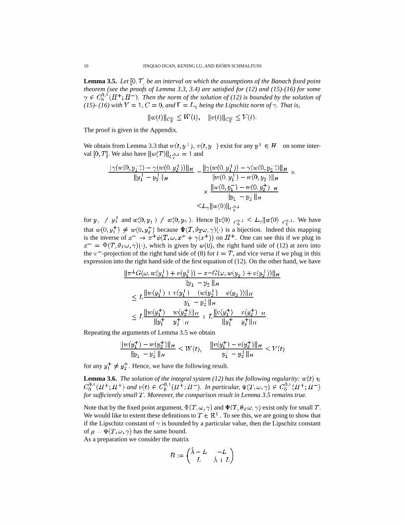
Lemma 3.5. Let� � � � � be an interval on which the assumptions of the Banach fixed point
theorem (see the proofs of Lemma 3.3, 3.4) are satisfied for (12) and (15)-(16) for some 0 � �# -� A * � A + � . Then the norm of the solution of (12) is bounded by the solution of
(15)- (16) with � � 4 , � � � , and � �87 � being the Lipschitz norm of . That is,� � � ��� � �� $ � � � �*��� � ��� � �� $ � � � �The proof is given in the Appendix.
We obtain from Lemma 3.3 that � �H� � * � � �� �H�� * � exist for any
� * 0 A * on some inter-val
� � � � � . We also have� � � ����� ��� #� �%4 and� � �!�� *- � � = � �� �� */ � �@� B� � *- = � */ � B �
� � �� �� *- � � = � � � � */ � �@� B� � � � � *- � = � � � � */ �@� B �
�� � � � � *- �&= � �� � � */ ��� B� � *- = � */ � B$ 7 � � � � �@��� ��� #�
for� *- �� � */
and � �� � � *- � �� � �!�� */ � . Hence
��� � �@��� ��� #� $ 7 � � � ����@��� ��� #� . We have
that � �!�� *- � �� � �� � � */ � because
� � � � � ; � � �< � is a bijection. Indeed this mapping
is the inverse ofI * � � * �� � � ; ��I * )I * � � on A * . One can see this if we plug inI * � �
� � � � ; � � �< � , which is given by � ����
, the right hand side of (12) at zero intothe � * -projection of the right hand side of (8) for
� ��
, and vice versa if we plug in thisexpression into the right hand side of the first equation of (12). On the other hand, we have� � > �� ; � � � *- � �� � *- � � = � > �� ; � � � */ � �� � */ � �@� B� � *- = � */ � B
$ 7 � � � *- � �� � *- � = � � */ � �� � */ � ��� B� � *- = � */ � B$ 7 � � � *- � = � � */ ��� B� � *- = � */ � B 7 � �� � *- �&= � � */ �@� B� � *- = � */ � B �
Repeating the arguments of Lemma 3.5 we obtain� � � *- �5= � � */ �@� B� � *- = � */ � B $ � � �H� ��� � *- �5= �� � */ �@� B� � *- = � */ � B $ � � �
for any� *- �� � */
. Hence, we have the following result.
Lemma 3.6. The solution of the integral system (12) has the following regularity: � � � 0
� �# -� A *�� A * � and
�� � � 0 � �# -� A *�� A + � . In particular,
� � ; � � 0 � �
# -� A *�� A + �
for sufficiently small
�. Moreover, the comparison result in Lemma 3.5 remains true.
Note that by the fixed point argument,
� � ; � � and�
� � � � ; � � exist only for small
�.
We would like to extent these definitions to
� 0 � * . To see this, we are going to show thatif the Lipschitz constant of is bounded by a particular value, then the Lipschitz constantof � � � � ; � � has the same bound.As a preparation we consider the matrix
� � �� �� = 7 = 77 �� 7��
INVARIANT MANIFOLDS FOR STOCHASTIC PARTIAL DIFFERENTIAL EQUATIONS 11
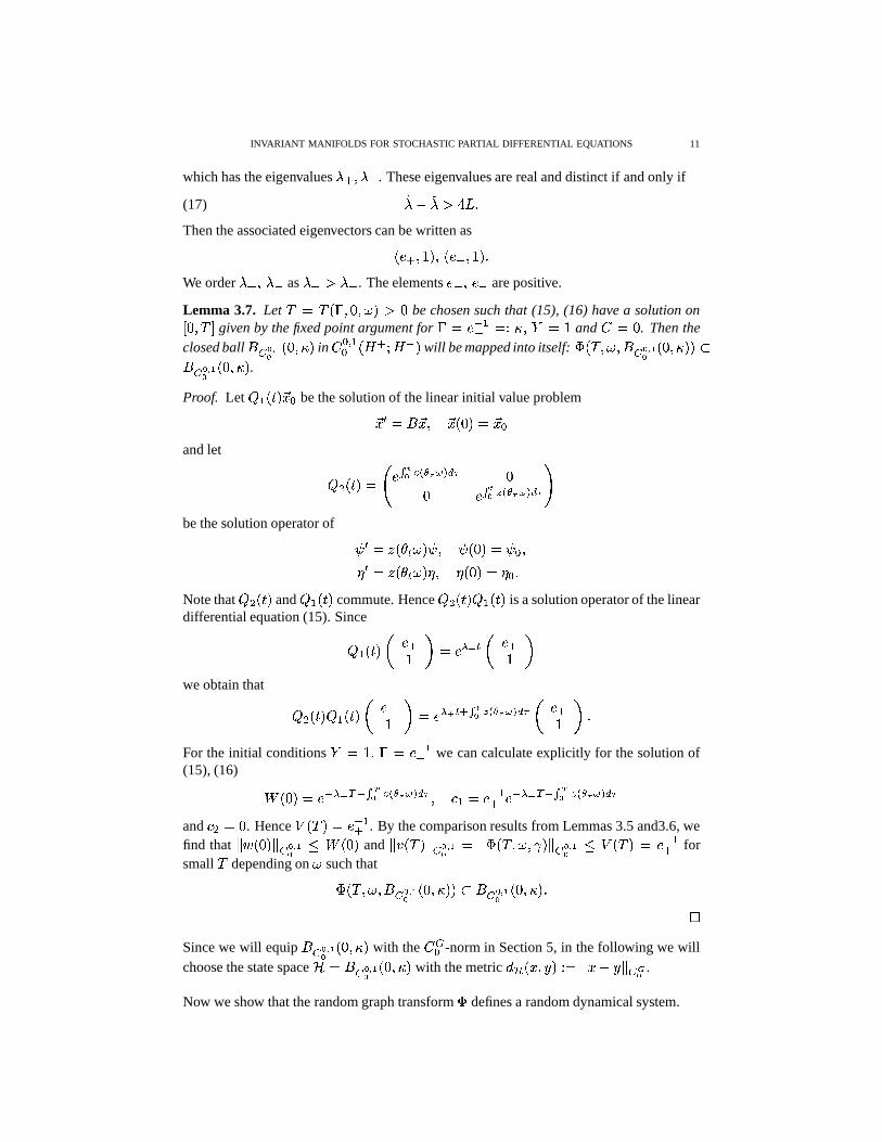
which has the eigenvalues� * � � + . These eigenvalues are real and distinct if and only if
��K='�� �� 7 �(17)
Then the associated eigenvectors can be written as &"* � 4 � � & + � 4 � �
We order� * ��� + as
� * 8� + . The elements & * � & + are positive.
Lemma 3.7. Let
��
� � � � � ; � � be chosen such that (15), (16) have a solution on� � � � � given by the fixed point argument for ��� & + -* � ��� � � � 4 and � � � . Then the
closed ball � � � � #� �� � � � in � �# -� A *�� A + � will be mapped into itself:
� � ; � � � ��� #� �!� � � �U>� � ��� #� �!� � � .
Proof. Let � - � ���I � be the solution of the linear initial value problem�I M � � �I5���I ���� � �I �and let � / � � � � & � �� �
�$�&! � �P �
� & �#�� ��$� ! � �
P be the solution operator of � M � �� � � ; �
� � � � � �
�� �� M � �� � � ; � � � � � � � � � �
Note that � / � � and � - � � commute. Hence � / � � � - � � is a solution operator of the lineardifferential equation (15). Since� - � � � &�*4 � � & ) � � � &"*4 �we obtain that � /� � � � - � � � &"*4 � � & ) � �)* � �� �
� �&! � �P � &�*4 � �
For the initial conditions � ��4 � � � & + -* we can calculate explicitly for the solution of(15), (16)
� ���� � & + ) � � + � �� ��$�&! � �
P �� - � & + -* & + ) � � + � �� ��$�&! � �
P and
/ � � . Hence � �� � & + -* . By the comparison results from Lemmas 3.5 and3.6, we
find that� � ������� ��� #� $ � � �
and� �� � �@��� ��� #� � � � � ; � ����� � � #� $ �
�� � & + -* for
small
�depending on ; such that
� � ; � � � ��� #� �!� � � �U> � � � � #� �� � � � �
�Since we will equip � � ��� #� �!� � � with the � �� -norm in Section 5, in the following we willchoose the state space � � � � � � #� �� � � � with the metric
��� 3I � � � � � �HIK= � � � �� .
Now we show that the random graph transform
defines a random dynamical system.
12 JINQIAO DUAN, KENING LU, AND BJORN SCHMALFUSS
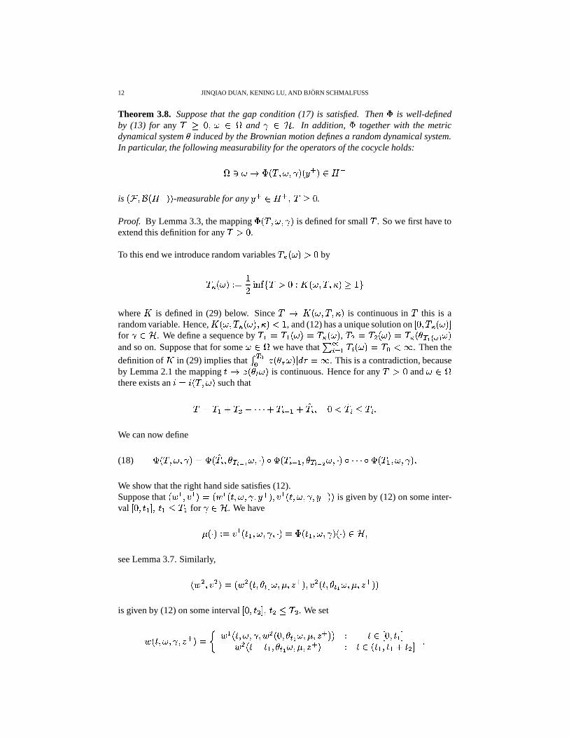
Theorem 3.8. Suppose that the gap condition (17) is satisfied. Then
is well-definedby (13) for any
� � � � ; 0 �and 0 � . In addition,
together with the metric
dynamical system � induced by the Brownian motion defines a random dynamical system.In particular, the following measurability for the operators of the cocycle holds:
� � ; �� � � ; � � � * � 0 A +
is 3�9�.2 A + � � -measurable for any
� * 0 A * �� � �
.
Proof. By Lemma 3.3, the mapping
� � ; � � is defined for small
�. So we first have to
extend this definition for any
� �.
To this end we introduce random variables
��� ; �" � by
� � ; � � � 4� ����� � � � � ; � � � � � � 4
where�
is defined in (29) below. Since
� � � ; � � � � � is continuous in
�this is a
random variable. Hence,� ; � � � ; � � � �"! 4 , and (12) has a unique solution on
� � � � � ; � �for 0 � . We define a sequence by
� - �� - ; � �
� � ; � ,
� / �� / ; � �
� � � � # � � � ; �
and so on. Suppose that for some ; 0 �we have that � � - � � ; � � �
� !�. Then the
definition of�
in (29) implies that � � �� � �� � ; �@� �EC � . This is a contradiction, because
by Lemma 2.1 the mapping� � � ����; � is continuous. Hence for any
� �and ; 0L�
there exists an � � � � � ; � such that��
� - � / �< << � � + - �� � � � ! �� � $ � � �We can now define
� � ; � � � �� � � � ��� # ; � < � % � � + - � � ���� (H; �< � % << < %
� - � ; � � �(18)
We show that the right hand side satisfies (12).Suppose that
� - ��� - � � � - �H� ; � � � * � ��- �H� ; � � � * � � is given by (12) on some inter-
val� � � ��- � � �.- $ � -
for 0 � . We have
� +< � � � � - �.-�� ; � � < � � �.-�� ; � � +< �U0 � �see Lemma 3.7. Similarly,
�/ ��� / � � �
/ �H� �"�$#�; � � � � * �H��� / �H� �"�$# ; � � � � * � �is given by (12) on some interval
� � � ��/ � � �+/ $ � /. We set
� �H� ; � � � * � � �
- �H� ; � � �/ �!� ���$#.; � � � � * � � � �U0 � �!� � - �
�/ �5= � - � ���$# ; � � � � * � � �U0 � - � � - � / �
�
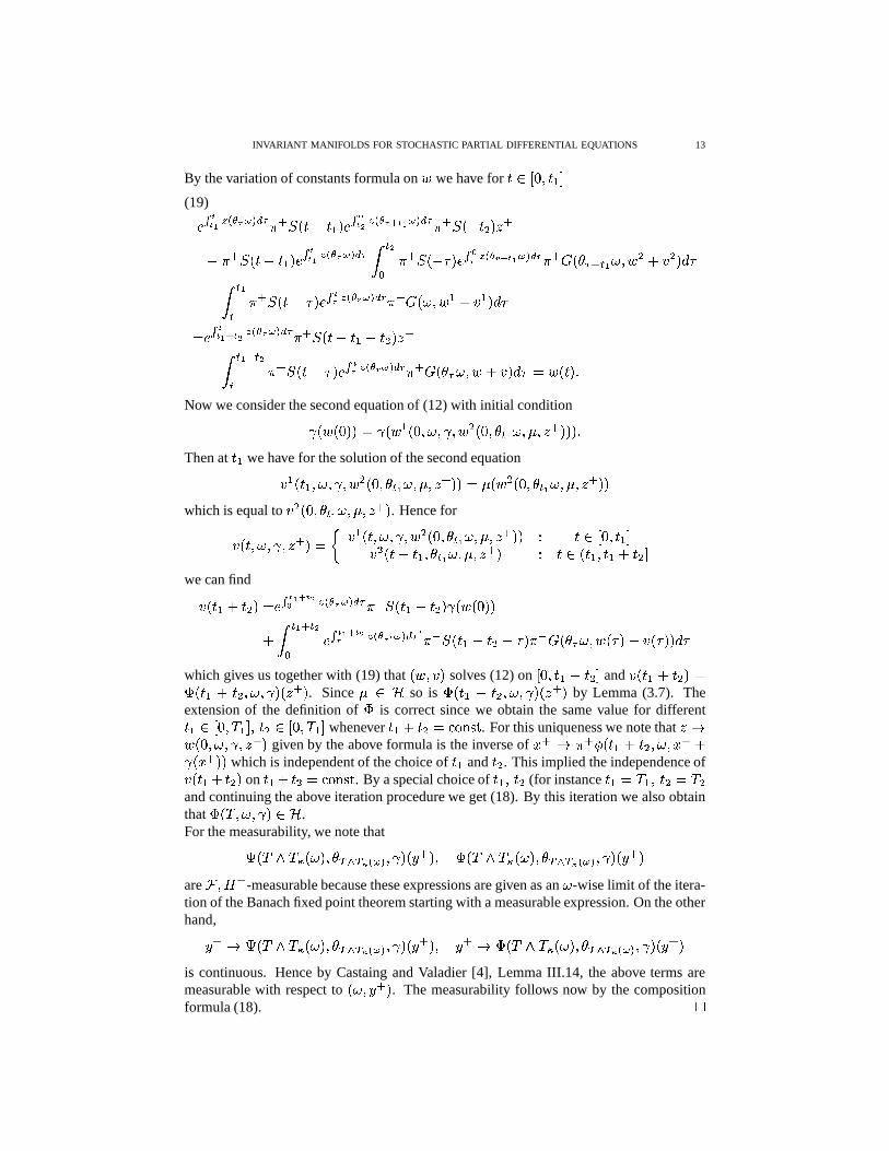
INVARIANT MANIFOLDS FOR STOCHASTIC PARTIAL DIFFERENTIAL EQUATIONS 13
By the variation of constants formula on � we have for� 0 � �!� � - �
& � �� # �� � ! � �
P � * � �5= �.- � & � �� ( ��$� ! �
� #� �P � * � += �+/ ��� *
= � * � � = �.- � & ���� # �� � ! � �
P B � (� � * � +=�C � &�� �! �
� � % �� #
� �P(' � * �� � *,� # ; � �
/ � / � �EC= B �$#
� � * � � =�C � &�� �! ��$�&% � �
P(' � * �� ; � � - � - � �EC� & �#�� #
�� ( �� �&! � �
P � * � �5= � - = � / � � *= B �$# *,�)(
� � * � �5= C � & � �! �� � % � �
P(' � * �� � ; � � �� � �EC � � � � �
(19)
Now we consider the second equation of (12) with initial condition � � � � � � - � � ; � � �
/ �!� � � #.; � � � � * � � � �Then at
��-we have for the solution of the second equation
� - � - � ; � � �/ � � ���$#�; � � � � * � � � � � / �� � �"�$#�; � � � � * � �
which is equal to� / �� � �"�$#�; � � � � * � . Hence for
� �H� ; � � � * � � � - �H� ; � � �
/ �!� ���$#.; � � � � * � � � �U0 � �!� � - �� / �5= � - � ���$# ; � � � � * � � �U0 � - � � - � / �we can find� � - �� / � � &�� � #
�� (� �� �&! � �
P � + � � - �� / � � ��� ��B � # *,� (� & � � #
�� (! �� � ! � � �
P � �,+�� � - �� / = C � �,+ �� � ; � � DC � � DC � � ��C
which gives us together with (19) that � �� � solves (12) on
� �!� � - � / � and�� � - � / � � � - � / � ; � � � * � . Since � 0 � so is
� - � / � ; � � � * � by Lemma (3.7). Theextension of the definition of
is correct since we obtain the same value for different�.- 0 � �!� � - � � �+/ 0 � �!� � - � whenever��- �+/ ��� � � ��� . For this uniqueness we note that
� �� �� � ; � � � * � given by the above formula is the inverse of
I * � � * �� �.- �+/D� ; ��I * )I * � � which is independent of the choice of� -
and�+/
. This implied the independence of� �.- �+/ �on�.- �+/ ��� � � ��� . By a special choice of
��-�� �+/(for instance
�.- �� -�� �+/ �
� /and continuing the above iteration procedure we get (18). By this iteration we also obtainthat
� � ; � �'0 � .
For the measurability, we note that�
��� � ; �H� � ��� ��� � � � � � � * �H�
��� � ; �H� � �� ��� � � � � � � * �
are��� A > -measurable because these expressions are given as an ; -wise limit of the itera-
tion of the Banach fixed point theorem starting with a measurable expression. On the otherhand,� * ���
��� � ; �H� � ��� ��� � � � � � � * �H� � * ��
��� � ; �H� � ��� ��� � � � � � � * �
is continuous. Hence by Castaing and Valadier [4], Lemma III.14, the above terms aremeasurable with respect to
; �� * � . The measurability follows now by the compositionformula (18). �
14 JINQIAO DUAN, KENING LU, AND BJORN SCHMALFUSS
Remark 3.9. i) Note that the solution of (15), (16) can be extended to any time interval� � � � � . Then lemma 3.5, 3.5 remain true for any
� �.
ii) Similar to the extension procedure we can show that�
� � ; � � is defined for any
� �!� ; 0J� and 0 � .
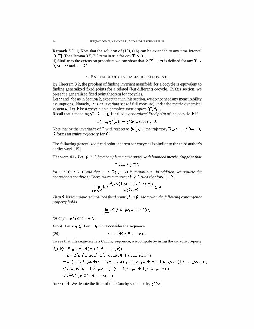
4. EXISTENCE OF GENERALIZED FIXED POINTS
By Theorem 3.2, the problem of finding invariant manifolds for a cocycle is equivalent tofinding generalized fixed points for a related (but different) cocycle. In this section, wepresent a generalized fixed point theorem for cocycles.Let
�and � be as in Section 2, except that, in this section, we do not need any measurability
assumptions. Namely,�
is an invariant set (of full measure) under the metric dynamicalsystem � . Let
be a cocycle on a complete metric space
��'� �����.
Recall that a mapping � � � ���is called a generalized fixed point of the cocycle
if
�H� ; � � ; � � � �� �"��; � for�'0 � �
Note that by the invariance of�
with respect to � � ����� , the trajectory � � � � � � � ; �U0�forms an entire trajectory for
.
The following generalized fixed point theorem for cocycles is similar to the third author’searlier work [19].
Theorem 4.1. Let ��'� �����
be a complete metric space with bounded metric. Suppose that �H� ; ��� �U>��
for ; 0 ��� � � �and that
IG� �H� ; �.I�� is continuous. In addition, we assume thecontraction condition: There exists a constant ! � such that for ; 0J�
��� � � � � ������ ��� 4 � ; �.I��H�� 4 � ; �� � ���� )I � � � $ �
Then
has a unique generalized fixed point � in�
. Moreover, the following convergenceproperty holds
� ����� �H� � + �$; �.I�� � � ; �
for any ; 0J� andIT0��
.
Proof. LetIT0 �
. For ; 0E� we consider the sequence� � � � � +�� ; ��I � � �(20)
To see that this sequence is a Cauchy sequence, we compute by using the cocycle property� � � � � +�� ; ��I �H�� � 4 � � +�� + - ; ��I � �
� � � � � � +�� ; �.I�� �� � � � +�� ; �� 4 � � +�� + - ; ��I � � �� � � 4 � � + - ; �� � = 4 � � +�� ; ��I � � �� 4 � � + - ; �� � = 4 � � +�� ; �� 4 � � +�� + - ; ��I�� � � �$ &�� ��� � = 4 � � +�� ; ��I �H�� � = 4 � � +�� ; �� 4 � � +�� + - ; ��I � � �$ & ��� ��� )I �� 4 � � +�� + - ; ��I � �
for � 0�� . We denote the limit of this Cauchy sequence by � ; � .
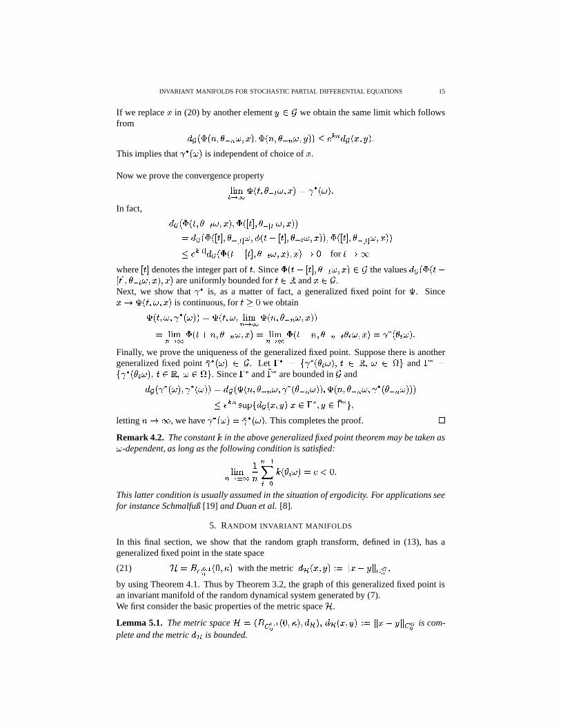
INVARIANT MANIFOLDS FOR STOCHASTIC PARTIAL DIFFERENTIAL EQUATIONS 15
If we replaceI
in (20) by another element�60 �
we obtain the same limit which followsfrom
� � � � � +�� ; ��I �H�� � � � +�� ; � � � �"$ & ��� � � )I �� � �This implies that � ; � is independent of choice of
I.
Now we prove the convergence property� � ���
�H� � + � ; ��I � � � ; � �In fact,
��� �H� � + ��; �.I��H�� "� � � � � + � � � ; �.I�� �� ��� "� � � � � + � � � ; � � � = � � � � � + ��; ��I � �H�� "� � � � � + � � � ; �.I�� �$ &�� � � � ��� � = � � � � � + �$; �.I�� ��I��'� �
for� �
where� � � denotes the integer part of
�. Since
� = � � � � � + ��; ��I � 0 � the values��� �&=� � � � � + � ; ��I �H��I � are uniformly bounded for
�U0 � andIT0 �
.Next, we show that � is, as a matter of fact, a generalized fixed point for
. SinceI9�� �H� ; �.I�� is continuous, for
�/� �we obtain
�H� ; � � ; � � � �H� ; � � ���� �
� � � +�� ; ��I � �� � ���� �
� � � � +�� ; ��I�� � � ���� �
� � � � +�� + ������; ��I � � �� �"��; � �Finally, we prove the uniqueness of the generalized fixed point. Suppose there is anothergeneralized fixed point 6 � ; � 0 �
. Let � � � � �"��; � � � 0 � � ; 0 � and 6� � � 6 � ����; �H� �U0 � � ; 0J� . Since � � and 6� � are bounded in
�and
� � �� ; �H� 6�� ; � � � � � � � � +�� ; � �� � +�� ; � � �� � � � +�� ; � 6�� � +�� ; � � �$ & ��� � ��� ��� 3I � � ��� I60 � � � � 0 6� � �letting � �
, we have � ; � � 6 � ; � . This completes the proof. �Remark 4.2. The constant in the above generalized fixed point theorem may be taken as; -dependent, as long as the following condition is satisfied:
� ���� � > 4
�� + -� � � � � ; � � ! � �
This latter condition is usually assumed in the situation of ergodicity. For applications seefor instance Schmalfuß [19] and Duan et al. [8].
5. RANDOM INVARIANT MANIFOLDS
In this final section, we show that the random graph transform, defined in (13), has ageneralized fixed point in the state space� � � � ��� #� �!� � � with the metric
��� )I �� � � � �HIK= � � ���� �(21)
by using Theorem 4.1. Thus by Theorem 3.2, the graph of this generalized fixed point isan invariant manifold of the random dynamical system generated by (7).We first consider the basic properties of the metric space � .
Lemma 5.1. The metric space � � � � � � #� �� � � � � � � �H� � � 3I �� � � � �HI = � � � �� is com-plete and the metric
� �is bounded.
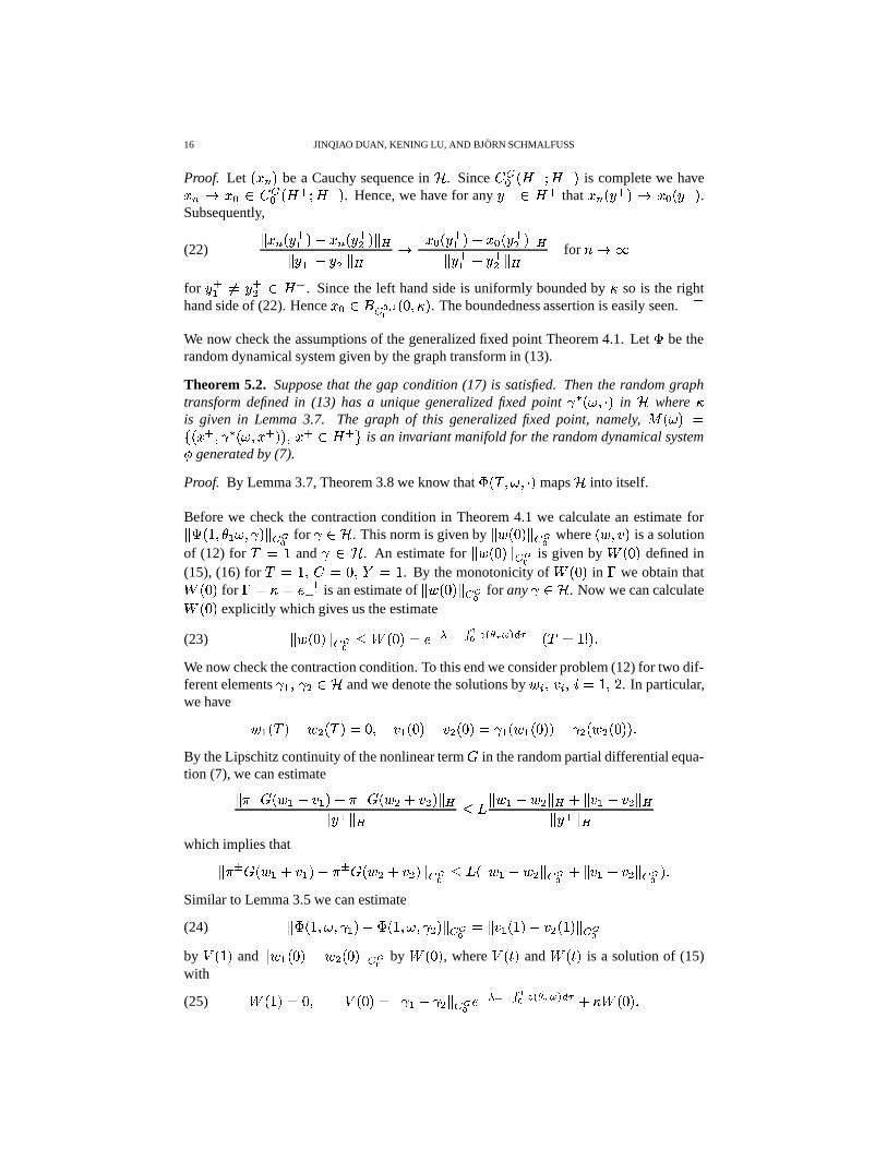
16 JINQIAO DUAN, KENING LU, AND BJORN SCHMALFUSS
Proof. Let 3I��
be a Cauchy sequence in � . Since � �� A *�� A + � is complete we haveI�� I � 0 ���� A *�� A + � . Hence, we have for any
� * 0 A * thatI� � * � � I � � * � .
Subsequently,�HI� � *- � = I
� � */ �@� B� � *- = � */ � B � � I � � *- � = I � � */ �@� B� � *- = � */ � B for � �
(22)
for� *- �� � */ 0 A * . Since the left hand side is uniformly bounded by � so is the right
hand side of (22). HenceI � 0 � � ��� #� �!� � � . The boundedness assertion is easily seen. �
We now check the assumptions of the generalized fixed point Theorem 4.1. Let
be therandom dynamical system given by the graph transform in (13).
Theorem 5.2. Suppose that the gap condition (17) is satisfied. Then the random graphtransform defined in (13) has a unique generalized fixed point � ; � < � in � where �is given in Lemma 3.7. The graph of this generalized fixed point, namely, � ; � � )I * � � ; �.I * � �H� I * 0 A * is an invariant manifold for the random dynamical system�
generated by (7).
Proof. By Lemma 3.7, Theorem 3.8 we know that
� � ; �< � maps � into itself.
Before we check the contraction condition in Theorem 4.1 we calculate an estimate for� � 4 � � - ; � �@� � �� for 0 � . This norm is given by� � � �@� � �� where
� ����� is a solutionof (12) for
�� 4 and 0 � . An estimate for
� � ������ ���� is given by� ���
defined in(15), (16) for
���4 � � � �!� � � 4 . By the monotonicity of
� ����in � we obtain that� ����
for � � � � & + -* is an estimate of� � � �@� � �� for any 0 � . Now we can calculate� ����
explicitly which gives us the estimate� � ����� ���� $ � ���� � &E+ ) � + � #� �� � ! � �
P ��'4�� � �(23)
We now check the contraction condition. To this end we consider problem (12) for two dif-ferent elements - � / 0 � and we denote the solutions by � � � � � � � � 4 � � . In particular,we have
� - ��5= � /
�� � �!� � - ���� = � / ���� � - � - ���� � = / � / ���� � �
By the Lipschitz continuity of the nonlinear term�
in the random partial differential equa-tion (7), we can estimate� � > �� � - �� - �5= � > �� � / � / �@� B� � * � B $ 7 � � - = � / � B ��� - = � / � B� � * � Bwhich implies that� �?> �� � - �� - � = �?> �� � / � / ��� ���� $ 7 � � - = � / � � �� ��� - = � / � � �� � �Similar to Lemma 3.5 we can estimate� 4 � ; � - �5= 4 � ; � / �@� ���� � � � - 4 � = � /� 4 �@� � ��(24)
by � 4 � and� � - � �'= � / ����� ���� by
� � �, where � � � and
� � �is a solution of (15)
with� 4 � � � � � ���� � � - = / � � �� & + ) � + � #� �
� � ! � �P � � ��� �
(25)
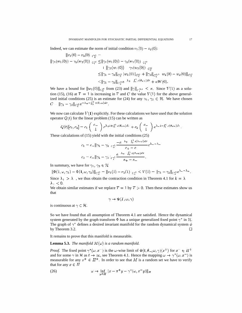
INVARIANT MANIFOLDS FOR STOCHASTIC PARTIAL DIFFERENTIAL EQUATIONS 17
Indeed, we can estimate the norm of initial condition� - � �5= � / � �
:��� - ���5= � / ����� ���� �� - � - ���� �&= / � / � � ��� � �� $ � - � - ��� � = / � - ���� �@� ���� � / � - � � � = /� � / ��� �@� � ��$ � -'= /E� ���� � � - � �@� ���� � /���� � � #� � � - � �5= � / � �@� ����$ � - = / � ���� &E+ ) � + � #� ��$�&! � �
P � � ��� �We have a bound for
� � - ����� ���� from (23) and� ��� � � #� $ � . Since � 4 � as a solu-
tion (15), (16) at
�� 4 is increasing in � and � the value � 4 � for the above general-
ized initial conditions (25) is an estimate for (24) for any - � / 0 � . We have chosen� � � - = / � ���� & + ) � + � #� �
�$� ! � �P .
We now can calculate � 4 � explicitly. For these calculations we have used that the solutionoperator � � � for the linear problem (15) can be written as� � �� - � / � � - � &�*4 � & ) � �)* � �� �
� � ! � �P / � & +4 � & ) �)* � �� �
� � ! � �P �
These calculations of (15) yield with the initial conditions (25) - � & + � - = / � ���� = & + )� + � #� �
�$� ! � �P & * = & + & ) + ) � / � &�* � - = / � ���� & + )
� + � #� �� � ! � �
P & * = & +�
In summary, we have for -�� / 0 �� 4 � ; � - �5=� 4 � ; � / �@� � �� � ��� - 4 �5= � / 4 ��� ���� $ � 4 � � � - = / � � �� & ) + ) � �Since
� * %� + , we thus obtain the contraction condition in Theorem 4.1 for � � + =� * ! � .We obtain similar estimates if we replace
�� 4 by
� ��. Then these estimates show us
that �� � � ; � �
is continuous at 0 � .
So we have found that all assumption of Theorem 4.1 are satisfied. Hence the dynamicalsystem generated by the graph transform
has a unique generalized fixed point � in � .
The graph of � defines a desired invariant manifold for the random dynamical system�
by Theorem 3.2. �It remains to prove that this manifold is measurable.
Lemma 5.3. The manifold � ; � is a random manifold.
Proof. The fixed point � ; ��I * � is the ; -wise limit of �H� � + ��; � � )I * � for
I * 0 A *and for some in � as
�U� , see Theorem 4.1. Hence the mapping ; � � ; ��I * � is
measurable for anyI * 0 A * . In order to see that � is a random set we have to verify
that for anyIJ0 A
; � ������ � B�HI = � * �8= � ; � � * � �@� B(26)

18 JINQIAO DUAN, KENING LU, AND BJORN SCHMALFUSS
is measurable, see Castaing and Valadier [4] Theorem III.9. Let A�� be a countable denseset of the separable space A . Then the right hand side of (26) is equal to
� � �� � B �� IK= � * � = � ; � � * � ��� B(27)
which follows immediately by the continuity of � ; � < � . The measurability of (27) followssince ; � � ; � � * � � is measurable for any
� 0 A . �Under the additional assumption �� ��: ��
we can show that � is an unstable manifolddenoted by � * : For any ; 0 ��� �����
andI 0 � * ; � there exists an
I + � 0 � � + � ; �such that
�� �H� � + ��; ��I + � � � I � I * �� ; ��I * �(28)
andI + � tends to zero. We setI + � � � �H� ; � �� � )I * � � � + ��; ��� �H� ; � � � 3I * � �H� I * � � � * I �
Equation (28) is satisfied becauseI * � � * �� �H� � + ��; �.I * � )I * � � is the inverse ofI * � � �H� ; � � � 3I * � , and because � is the fixed point of the graph transform. The
value� � �H� � � ; � � � )I * �@� ���� can be estimated by
� ����a solution of (15), (16) on
� �!� � �with � � � � � � � and � � 4 and ; � � + � ; .
� � �can be calculated explicitly for any� �
. Hence � � �H� ; � �� � )I * �@� B $ & + ) � � + � �� �� �&! � �
P �HI * � B �(We have to replace ; by � + � ; !) We can derive from Lemma 2.1 iv)B �
+ ��� � ;
� �EC !�� �for any
� �if�
is chosen sufficiently large depending on ; and�. Hence
� � �H� ; � � � )I * �@� � ��tends to zero exponentially. On the other hand we have for � 0 �� �� � + ��; ��� �H� ; � �� � )I * � ��� B%$ � � � �H� ; � �� � 3I * ��� BQ� �
for�&� �
This convergence is exponentially fast. We conclude that � * is the unstable manifold for(7).
However, our intention is to prove that (4) has an invariant (unstable) manifold. On accountof conjugacy of (4) and (7) by (9) and (10) we will now formulate the following result.
Theorem 5.4. Let�
by the random dynamical system generated by (7) and �� be the so-lution version of (4) generated by (11). Then � ; � is the invariant manifold of
�if and
only if �� * ; � �� + - ; � � * ; � � is the invariant manifold of �� . Moreover, if � * is an
unstable manifold, then so is �� * .
Proof. We have the relationship between�
and �� given in Lemma 2.2�� �H� ; � �� * ; � � �� + - � � ; � �� �H� ; � � ; � �� * ; � � � �
�� + - � � ; � �� �H� ; � � * ; � � �U>
� + - � � ; � � * � � ; � � � �� * � � ; � �Note that
� � �� � � ; � has a sublinear growth rate, see Lemma 2.1iii). Thus the transform� + - � + � ; � does not change the exponential convergence of� �H� ; � � ; � � )I * � :�� �H� ; � � � ; � � �� + - � + ��; ��� �H� ; �
� ; � � � ; � � � �H� � � ; � � �
� + - ; � � ; � � �It follows that �� * ; � is unstable. �
INVARIANT MANIFOLDS FOR STOCHASTIC PARTIAL DIFFERENTIAL EQUATIONS 19
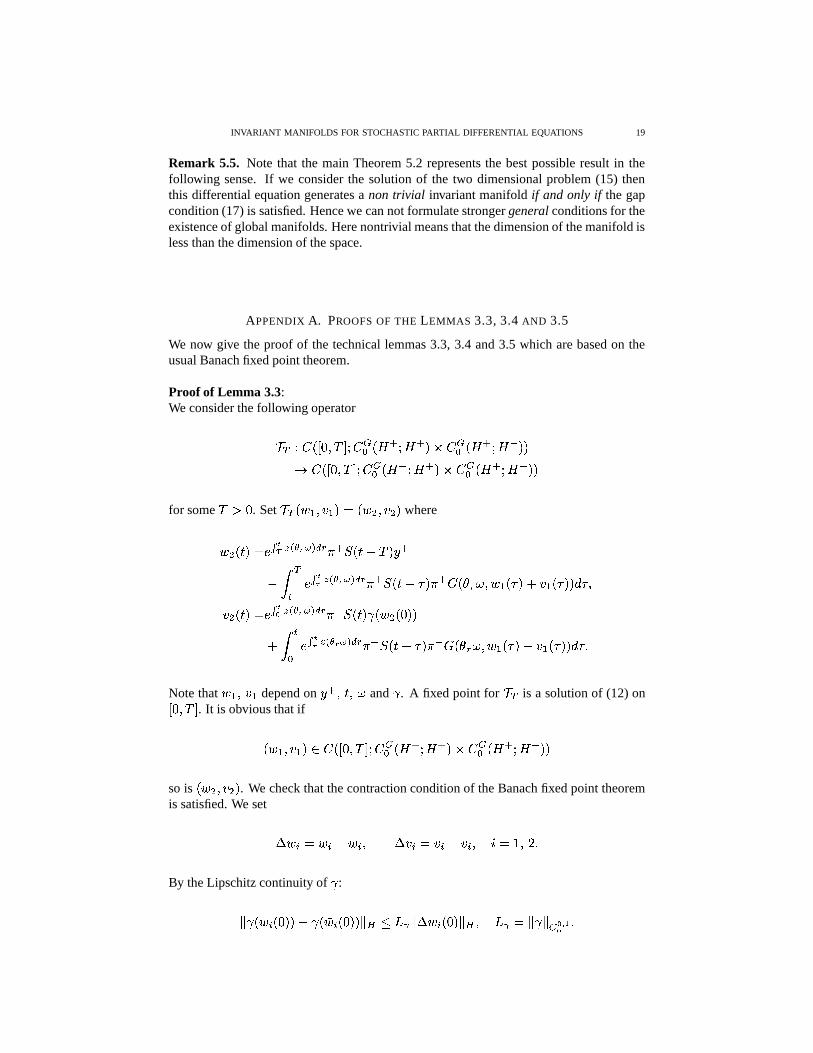
Remark 5.5. Note that the main Theorem 5.2 represents the best possible result in thefollowing sense. If we consider the solution of the two dimensional problem (15) thenthis differential equation generates a non trivial invariant manifold if and only if the gapcondition (17) is satisfied. Hence we can not formulate stronger general conditions for theexistence of global manifolds. Here nontrivial means that the dimension of the manifold isless than the dimension of the space.
APPENDIX A. PROOFS OF THE LEMMAS 3.3, 3.4 AND 3.5
We now give the proof of the technical lemmas 3.3, 3.4 and 3.5 which are based on theusual Banach fixed point theorem.
Proof of Lemma 3.3:We consider the following operator
� � ��� � �!��
� � � �� A * � A * � � � �� A * � A�+ � �� � � �!��
� � � �� A * � A * � � � �� A * � A + � �for some
� �. Set
� � � - ��� - � � � / �� / � where
� / � � � &��#�� �� �&% � �
P(' � * � � = �� � *
= B �� &�� �! �
� �&% � �P(' � * � � =�C � � * �� � ; � � - DC ���� - DC � � �EC �
� / � � � &�� �� ��$�&% � �
P(' �,+�� � � � / ��� �;B �
� &����! �� �"% � �
P(' �,+ � �5=�C � �,+ �� � ; � � - DC � � - DC � � ��C �Note that �
-�� � -depend on
� * � �H� ; and . A fixed point for� � is a solution of (12) on� � � � � . It is obvious that if
� - �� - �U0 � � �!��
� � � �� A * � A * � � � �� A * � A + � �so is
� / �� / � . We check that the contraction condition of the Banach fixed point theoremis satisfied. We set
� � � � � � = 6� � � � � � � � � = 6� � � � �'4 � � �By the Lipschitz continuity of :
� � � ���� �&= 6� � ��� �@� B%$ 7 � � � � � ����� B8� 7 � � � ��� ��� #� �
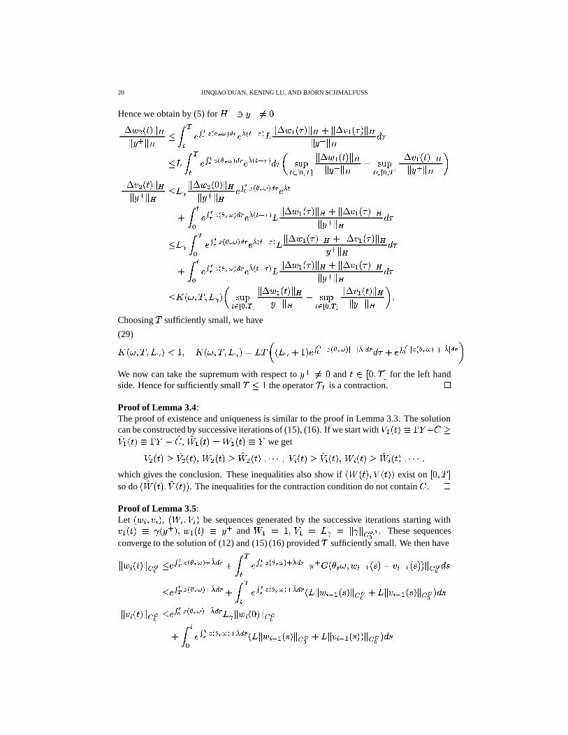
20 JINQIAO DUAN, KENING LU, AND BJORN SCHMALFUSS
Hence we obtain by (5) for A * � � * �� �� � � / � ��� B� � * � B $ B �� &��#�! �
� � % � �P(' &�() � � +� � 7 � � � - DC ��� B � � � - DC ��� B� � * � B �EC
$ 7 B �� &�� �! ��$�&% � �
P('@& () � � + � ��C � ��� ���� � � # � �� � � - � �@� B� � * � B ��� ���� � � # � �
� � � - � �@� B� � * � B �� � � / � ��� B� � * � B $ 7 � � � � /� ����� B� � * � B & � �� �� � % � �
P(' & .) � B �
� &�� �! �� � % � �
P(' & .) � � +� � 7 � � � - DC ��� B � � � - DC ��� B� � * � B ��C$ 7 � B �� &�� �! �
� �"% � �P(' & () � � +� � 7 � � � - DC ��� B � � � - DC ��� B� � * � B ��C
;B �� & � �! �
� �"% � �P(' &�.) � � +� � 7 � � � - DC ��� B � � � - DC ��� B� � * � B ��C
$ � ; � � � 7 � � � � ������ � � # � �� � � - � ��� B� � * � B � ������ � � # � �
� � � - � �@� B� � * � B � �Choosing
�sufficiently small, we have
� ; � � � 7 � ��! 4 � � ; � � � 7 � � �87 � � 7 � 4 � &�� ���� �� �"% � �
� * � () � P(' �EC &�� ���� ��$�&% � �
� * � .) � P(' �(29)
We now can take the supremum with respect to� * �� �
and�80 � �!� � � for the left hand
side. Hence for sufficiently small
� $ 4 the operator� � is a contraction. �
Proof of Lemma 3.4:The proof of existence and uniqueness is similar to the proof in Lemma 3.3. The solutioncan be constructed by successive iterations of (15), (16). If we start with � - � ��� � � � ��� - � ��� �� � �� , �� - � � � � - � ��� � we get
� / � � � �� / � �H� � / � �"� �� / � �U�< < < � � � � �"� �� � � � � � � � � � �� � � �U� << < �which gives the conclusion. These inequalities also show if
� � � � � � � � exist on� �!� � �
so do �� � �H� �� � � � . The inequalities for the contraction condition do not contain � . �
Proof of Lemma 3.5:Let
� � ��� � � , � � � � � � be sequences generated by the successive iterations starting with� - � ��� � * � � � - � ��� � * and� - � 4 � � - � 7 � � � � � � � #� . These sequences
converge to the solution of (12) and (15) (16) provided
�sufficiently small. We then have� � � � �@� ���� $ &����� �
� �"% � � * () P(' ;B �� &�� �� �� �"% � � * () P(' � � * �� ���; � � � + - � � �� � + - � � ��� ���� � $ &����� �
� �"% � � * () P(' B �� &�� �� �� �"% � � * () P(' 7 � � � + - � ��� ���� 7 ��� � + - � �@� ���� � ��� � � � �@� ���� $ &����� �
� �"% � � * .) P('@7 � � � � ����@� � ��FB �
� &��#�� �� �&% � � * .) P(' 7 � � � + - � �@� � �� 7 � � � + - � � ��� ���� � ��
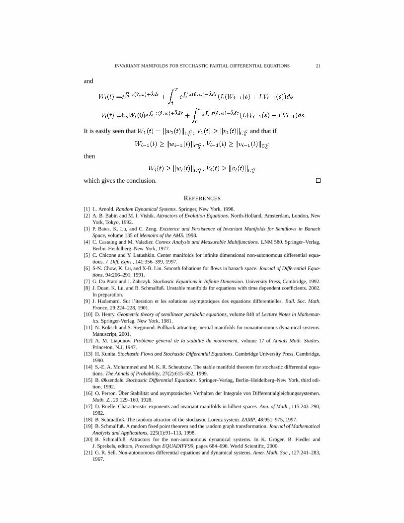
INVARIANT MANIFOLDS FOR STOCHASTIC PARTIAL DIFFERENTIAL EQUATIONS 21
and
� � � � � &����� �� �"% � � * () P(' ;B �� &�� �� �
� �"% � � * () P(' 7 � � + - � � 7�� � + - � � � ��� � � � � Ł �
� � ��� &�� �� �� �"% � � * .) P(' B �� &��#�� �
�$�&% � � * .) P(' 7 � � + - � � 7�� � + - � �� �It is easily seen that
� - � � � � � - � ��� ���� � � - � � � � � - � �@� ���� and that if� � + - � ��� � � � + - � ��� � �� � � � + - � � � � � � + - � �@� ����
then� � � ��� � � � � ��� � �� � � � � � � � � � � �@� ����
which gives the conclusion. �REFERENCES
[1] L. Arnold. Random Dynamical Systems. Springer, New York, 1998.[2] A. B. Babin and M. I. Vishik. Attractors of Evolution Equations. North-Holland, Amsterdam, London, New
York, Tokyo, 1992.[3] P. Bates, K. Lu, and C. Zeng. Existence and Persistence of Invariant Manifolds for Semiflows in Banach
Space, volume 135 of Memoirs of the AMS. 1998.[4] C. Castaing and M. Valadier. Convex Analysis and Measurable Multifunctions. LNM 580. Springer–Verlag,
Berlin–Heidelberg–New York, 1977.[5] C. Chicone and Y. Latushkin. Center manifolds for infinite dimensional non-autonomous differential equa-
tions. J. Diff. Eqns., 141:356–399, 1997.[6] S-N. Chow, K. Lu, and X-B. Lin. Smooth foliations for flows in banach space. Journal of Differential Equa-
tions, 94:266–291, 1991.[7] G. Da Prato and J. Zabczyk. Stochastic Equations in Infinite Dimension. University Press, Cambridge, 1992.[8] J. Duan, K. Lu, and B. Schmalfuß. Unstable manifolds for equations with time dependent coefficients. 2002.
In preparation.[9] J. Hadamard. Sur l’iteration et les solutions asymptotiques des equations differentielles. Bull. Soc. Math.
France, 29:224–228, 1901.[10] D. Henry. Geometric theory of semilinear parabolic equations, volume 840 of Lecture Notes in Mathemat-
ics. Springer-Verlag, New York, 1981.[11] N. Koksch and S. Siegmund. Pullback attracting inertial manifolds for nonautonomous dynamical systems.
Manuscript, 2001.[12] A. M. Liapunov. Probleme general de la stabilite du mouvement, volume 17 of Annals Math. Studies.
Princeton, N.J, 1947.[13] H. Kunita. Stochastic Flows and Stochastic Differential Equations. Cambridge University Press, Cambridge,
1990.[14] S.-E. A. Mohammed and M. K. R. Scheutzow. The stable manifold theorem for stochastic differential equa-
tions. The Annals of Probability, 27(2):615–652, 1999.[15] B. Øksendale. Stochastic Differential Equations. Springer–Verlag, Berlin–Heidelberg–New York, third edi-
tion, 1992.[16] O. Perron. Uber Stabilitat und asymptotisches Verhalten der Integrale von Differentialgleichungssystemen.
Math. Z., 29:129–160, 1928.[17] D. Ruelle. Characteristic exponents and invariant manifolds in hilbert spaces. Ann. of Math., 115:243–290,
1982.[18] B. Schmalfuß. The random attractor of the stochastic Lorenz system. ZAMP, 48:951–975, 1997.[19] B. Schmalfuß. A random fixed point theorem and the random graph transformation. Journal of Mathematical
Analysis and Applications, 225(1):91–113, 1998.[20] B. Schmalfuß. Attractors for the non-autonomous dynamical systems. In K. Groger, B. Fiedler and
J. Sprekels, editors, Proceedings EQUADIFF99, pages 684–690. World Scientific, 2000.[21] G. R. Sell. Non-autonomous differential equations and dynamical systems. Amer. Math. Soc., 127:241–283,
1967.
22 JINQIAO DUAN, KENING LU, AND BJORN SCHMALFUSS
[22] T. Caraballo, J. Langa and J. C. Robinson. A stochastic pitchfork bifurcation in a reaction-diffusion equation.2001. Submitted.
[23] M. I. Vishik. Asymptotic Behaviour of Solutions of Evolutionary Equations. Cambridge University Press,Cambridge, 1992.
[24] T. Wanner. Linearization random dynamical systems. In C. Jones, U. Kirchgraber and H. O. Walther, editors,Dynamics Reported, Vol. 4, 203-269, Springer-Verlag, New York, 1995.
(J. Duan) DEPARTMENT OF APPLIED MATHEMATICS, ILLINOIS INSTITUTE OF TECHNOLOGY, CHICAGO, IL60616, USAE-mail address, J. Duan: [email protected]
(K. Lu) DEPARTMENT OF MATHEMATICS, BRIGHAM YOUNG UNIVERSITY, PROVO, UTAH 84602, USAE-mail address, K. Lu: [email protected]
(B. Schmalfuß) DEPARTMENT OF SCIENCES, UNIVERSITY OF APPLIED SCIENCES, GEUSAER STRASSE,06217 MERSEBURG, GERMANY
E-mail address, B. Schmalfuß: [email protected]