Invariant Measures for Hybrid Stochastic Systems

Xavier Garcia∗ Jennifer Kunze† Thomas Rudelius‡

Anthony Sanchez§ Sijing Shao¶ Emily Speranza‖

Chad Vidden∗∗

August 9, 2012

Abstract

In this paper, we seek to understand the behavior of dynamical sys-tems that are perturbed by a parameter that changes discretely in time.If we impose certain conditions, we can study certain embedded systemswithin a hybrid system as time-homogeneous Markov processes. In par-ticular, we prove the existence of invariant measures for each embeddedsystem and relate the invariant measures for the various systems throughthe flow. We calculate these invariant measures explicitly in several illus-trative examples.

Keywords: Dynamical Systems; Markov processes; Markov chains;stochastic modeling

1 Introduction

An understanding of dynamical systems allows one to analyze the way pro-cesses evolve through time. Usually, such systems are given by differentialequations that model real world phenomena. Unfortunately, these modelsare limited in that they cannot account for random events that may occurin application. These stochastic developments, however, may sometimesbe modeled with Markov processes, and in particular with Markov chains.

∗Department of Mathematics, University of Minnesota - Twin Cities, Minneapolis, MN55455, USA (garci363@umn.edu). Research supported by DMS 0750986 and DMS 0502354†Department of Mathematics, Saint Mary’s College of Maryland, St Marys City, MD 20686,

USA (jckunze@smcm.edu). Research supported by DMS 0750986‡Department of Mathematics, Cornell University, Ithaca, NY 14850, USA

(twr27@cornell.edu). Research supported by DMS 0750986§Department of Mathematics, Arizona State University, Tempe, AZ 85281, USA

(Anthony.Sanchez.1@asu.edu). Research supported by DMS 0750986 and DMS 0502354¶Department of Mathematics, Iowa State University, Ames, IA 50014, USA

(sshao@iastate.edu). Research supported by Iowa State University‖Department of Mathematics, Carroll College, Helena, MT 59625, USA

(esperanza@carroll.edu). Research supported by DMS 0750986∗∗Department of Mathematics, Iowa State University, Ames, IA 50014, USA

(cvidden@iastate.edu). Research supported by Iowa State University.

1

We can unite the two models in order to see how these dynamical systemsbehave with the perturbation induced by the Markov processes, creating ahybrid system consisting of the two components. Complicating matters,these hybrid systems can be described in either continuous or discretetime.

The focus of this paper is studying the way these hybrid systems be-have as they evolve. We begin by defining limit sets for a dynamical systemand stochastic processes. We next examine the limit sets of these hybridsystems and what happens as they approach the limit sets. Concurrently,we define invariant measures and prove their existence for hybrid systemswhile relating these measures to the flow. In addition, we supply exampleswith visuals that provide insight to the behavior of hybrid systems.

2 The Stochastic Hybrid System

In this section, we define a hybrid system.

Definition 1. A Markov process Xt is called time-homogeneous on timeset T if, for all t1, t2, k ∈ T and for any sets A1, A2 ∈ S,

P (Xt1+k ∈ A1|Xt1 ∈ A2) = P (Xt2+k ∈ A1|Xt2 ∈ A2).

Otherwise, it is called time-inhomogeneous.

Definition 2. A Markov chain Xn is a Markov process for which pertur-bations occur on a discrete time set T and finite state space S.

For a Markov chain on the finite state space S with cardinality |S|, itis useful to describe the probabilities of transitioning from one state toanother with a transition matrix

Q ≡

P1→1 . . . P1→|S|. .. .. .

P|S|→1 . . . P|S|→|S|

where Pi→j is the probability of transitioning from state si ∈ S to statesj ∈ S.

Also, for the purposes of this paper, we suppose that our Markov chaintransitions occur regularly at times t = nh for some length of time h ∈ R+

and for all n ∈ N.

Definition 3. Let {Xn}, for Xn ∈ S and n ∈ N, be a sequence of statesdetermined by a Markov chain.

For t ∈ R+, define the Markov chain perturbation Zt = Xb thc, where⌊

th

⌋is the greatest integer less than or equal to t

h.

Note that Zt, instead of being defined only on discrete time values likea Markov chain, is instead a stepwise function defined on continuous time.

Definition 4. Given a compact, complete metric space M and state spaceS as above, define a dynamical system ϕ with random perturbation func-tion Zt, as given in Definition 3, by

ϕ : R+ ×M × S →M

2

with

ϕ(t, x0, Z0) = ϕZt(t− nh, ϕZnh(h, ...ϕZ2h(h, ϕZh(h, ϕZ0(h, x0)))))

where ϕZk represents the deterministic dynamical system ϕ evaluated instate Zk and nh is the largest multiple of h less than t.

For ease of notation, let

xt = ϕ(t, x0, Z0) ∈M

represent the position of the system at time t.

Definition 5. Let

Yt =

(xtZt

)define the hybrid system at time t. In other words, the hybrid systemconsists of both a position xt = ϕ(t, x0, Z0) ∈M and a state Zt ∈ S.

The ω-limit set has the following generalization in a hybrid system.

Definition 6. The stochastic limit set C(x) for an element of our statespace x ∈ M and the hybrid system given above is the subset of M withthe following three properties:

1. Given y ∈M and tk →∞ such that xtk → y, P (y ∈ C(x)) = 1.

2. C(x) is closed.

3. C(x) is minimal: if some set C′(x) has properties 1 and 2, thenC ⊆ C′.

3 The Hybrid System as a Markov Pro-cess

Lemma 7. Each of the following is a Markov process:(i) any deterministic dynamical system ϕ(t, x0) with time set R+.(ii) any Markov chain perturbation Zt with discrete time set contained inR+.(iii) the corresponding hybrid system Yt, as in Definition 5.

Proof. (i) Any deterministic system is trivially a Markov process, sinceϕ(t, x0) is uniquely determined by ϕ(τ, x0) at any single past time τ ∈ R+.

(ii) By definition, a Markov chain is a Markov process. However, theMarkov chain perturbation Zt is not exactly a Markov chain. A Markovchain exists on a discrete time set, in our case given by T = {t ∈ R+|t = nhfor some n ∈ N}; conversely, the time set of Zt is R+, with transitionsbetween states ocurring on the previous time set (that is, at t ≡ 0 modh). Despite this difference, Zt maintains the Markov property: we cancompute P (Zt ∈ A) for any set A based solely on Zτ1 and the values ofthe times t and τ1. Explicitly, the probability that Zt will be in state siat time t is given by

P (Zt = si) =(

(QT )n)ij

3

where n is the number of integer multiples of h (i.e. the number of tran-sitions that occur) between t and τ1. Clearly, this is independent of thestates Zτi for i > 1, so that the random perturbation is indeed a Markovprocess.

(iii) Now, keeping in mind that the hybrid system Yt consists of botha location xt ∈ M in the state space and a value Zt ∈ S of the randomcomponent, we can combine (i) and (ii) to see that the entire system isalso a Markov process. We see from (ii) that Zt follows a Markov process.Furthermore, P (xt ∈ Ax) at time t depends solely on the location xτ1 atany time τ1 < t and the states of the random perturbation sequence Zbetween t and τ1, regardless of any past behavior of the system. Hence,for any collection of sets Aα, α ∈ N,

P (Zt ∈ Az|Zτ1 ∈ Az1 , Zτ2 ∈ Az2 , ..., Zτn ∈ Azn) = P (Zt ∈ Az|Zτ1 ∈ Az1)

and

P (xt ∈ Ax|xτ1 ∈ Ax1 , xτ2 ∈ Ax2 , ..., xτn ∈ Axn) = P (xt ∈ Ax|xτ1 ∈ Ax1).

So,

P (Yt ∈ Ay|Yτ1 ∈ Ay1 , Yτ2 ∈ Ay2 , ..., Yτn ∈ Ayn) = P (Yt ∈ Ay|Yτ1 ∈ Ay1).

Thus, the hybrid system is a Markov process.

Unfortunately, the hybrid system is not time-homogeneous. Recallthat state transitions of Zt occur at times t = nh for n ∈ N. So, the stateof the system at time h

4uniquely determines the system at 3h

4, since there

is no transition in this interval. However, the system at time 5h4

is notdetermined uniquely by the system at 3h

4, since a stochastic transition

occurs at t = h ∈ [ 34, 5

4]. Therefore, with t1 = h

4, t2 = 3h

4, and k = 1

2,

P (Yh4 + 1

2∈ A|Yh

4∈ A0) 6= P (Y 3h

4 + 12∈ A|Y 3h

4∈ A0),

violating Definition 1. However, in order to satisfy the hypotheses ofthe Krylov-Bogolyubov theorem [3, 4] found in Theorem 14, the hybridsystem must be time-homogeneous.

To create a time-homogeneous system, we restrict the time set onwhich our Markov process is defined. Instead of allowing our time set{t, τ1, τ2, τ3, ..., τn} ⊂ R+ to be any decreasing sequence of real numbers,we create time sets t0 +nh for each t0 ∈ [0, h) and n ∈ N. In other words,we define a different time set for each value t0 < h with

{t ∈ R+|t = t0 + nh for some n ∈ N} .

We call the hybrid system on these multiple, restricted time sets the dis-crete system.

Proposition 8. The discrete hybrid system above is a time-homogeneousMarkov process.

Proof. First, we must show that the discrete hybrid system is a Markovprocess. This follows immediately from the proof that our original hybridsystem is a Markov process. Since the Markov property holds for allt, τ1, τ2, ..., τn ∈ R+, it must necessarily hold for the specific time sets

4

{t ∈ R+|∃n ∈ N such that t = t0 + nh}

for each t0 < h.Now, it remains to show that this system is time-homogeneous. Recall

that the time-continuous hybrid system failed to be time-homogeneousbecause its Zt component was not time-homogeneous. Although transi-tions occurred only at regular, discrete time values, a test interval couldbe of any length; an interval of size h

2, for example, might contain either

0 or 1 transitions. However, because our discrete system creates separatetime sets, any time interval - starting and ending within the same timeset - must be of length nh for some n ∈ N, and thus will contain preciselyn potential transitions. So, taking t1, t2 ∈ R+, we know

P (Yt1+nh ∈ A|Yt1 ∈ A0) = P (Yt2+nh ∈ A|Yt2 ∈ A0).

Note that the first component of the hybrid system, xt, is also time-homogeneous under the discrete time system. Given Zt, it can be treatedas a deterministic system, and therefore it is time-homogeneous. Thus,the discrete hybrid system is time-homogeneous.

4 Invariant Measures for the Hybrid Sys-tem

We now introduce several definitions that will lead us to the main resultsof this paper.

Definition 9. Consider a hybrid system Yt and a σ-algebra Σ on thespace M . A measure µ on M is invariant if, for all sets A ∈ Σ and alltimes t ∈ R+,

µ(A) =

∫x0∈M

P (xt ∈ A)µ(dx).

Definition 10. Let (M, T ) be a topological space, and let Σ be a σ-algebraon M that contains the topology T . Let M be a collection of probabilitymeasures defined on Σ. The collection M is called tight if, for any ε > 0,there is a compact subset Kε of M such that, for any measure µ in M,

µ(M\Kε) < ε.

Note that, since µ is a probability measure, it is equivalent to say µ(Kε) >1− ε.

The following definitions are from [3].

Definition 11. Let (M,ρ) be a separable metric space. Let {P(M)}denote the collection of all probability measures defined on M (with itsBorel σ-algebra). A collection K ⊂ {P(M)} of probability measures istight if and only if K is sequentially compact in the space equipped withthe topology of weak convergence.

Definition 12. Consider M with σ-algebra Σ. Let C0(M,R) denote theset of continuous functions from M to R. The probability measure P(t, x, ·)on Σ induces a map

Pt(x) : C0(M,R)→ R

5

with

Pt(x)(f) =

∫y∈M

f(y)P(t, x, dy).

Pt is called a Markov operator.

Definition 13. A Markov operator P is Feller if Pϕ is continuous forevery continuous bounded function ϕ : X → R. In other words, it is Fellerif and only if the map x 7→ P(x, ·) is continuous in the topology of weakconvergence.

We state the Krylov-Bogolyubov Theorem without proof.

Theorem 14. (Krylov-Bogolyubov) Let P be a Feller Markov op-erator over a complete and separable space X. Assume that there existsx0 ∈ X such that the sequence Pn(x0, ·) is tight. Then, there exists atleast one invariant probability measure for P.

We now show that the conditions of the theorem are satisfied by thediscrete hybrid system, yielding the existence of invariant measures as acorollary.

Lemma 15. Given t0 ∈ [0, h), the discrete hybrid system Markov opera-tors Pn for n ∈ N given by

Pnf(Y ) ≡∫M×S

f(Y1)P(nh, Y, dY1)

are Feller.

Proof. We begin by showing that P1 is Feller. By induction, it followsthat Pn is Feller for all n ∈ N. It is clear that there are only finitely manypossible outcomes of running the hybrid system for time h. Namely, thereare at most |S| possible outcomes, where |S| denotes the cardinality of S.Given

Y0 =

(x0

Z0 = si

)∈M × S,

the only possible outcomes at time t = 1 are

Y j1 =

(ϕj(t0, ϕi(h− t0, x))

sj

)for j ∈ {1, ..., |S|} where ϕi, ϕj are the flows of the dynamical systemscorresponding to states si and sj , respectively. The probability of the jth

outcome is given by Pi→j , the probability of transitioning from state sito state sj . Therefore,

P1f(Y ) =

∫M×S

f(Y1)P(h, Y, dY1) =

|S|∑j=1

Pi→jf(Y j1 )

Each ϕi is continuous under the assumption that each flow is con-tinuous with respect to its initial conditions. The map from si to sj iscontinuous since S is finite, so every set is open and hence the inverse im-age of any open set is open. The function f is continuous by hypothesis,and any finite sum of continuous functions is also continuous. ThereforeP1f is also continuous, and hence P1 is Feller.

6

We see now that the conditions of the Krylov-Bogolyubov Theorem(14) hold. Namely, because M and S are compact (the former by assump-tion, the latter since it is finite), M × S is compact. Thus, any collectionof measures is automatically tight, since we can take Kε = X. It is well-known that any compact metric space is also complete and separable.Applying Theorem 14 gives the following corollary, which is one of theprimary results of the paper.

Corollary 16. The discrete hybrid system has an invariant measure foreach t0 ∈ [0, h).

So, rather than speaking of an invariant measure for the time-continuoushybrid system, we can instead imagine a periodic invariant measure cy-cling continuously through h. That is, for each time t0 ∈ [0, h), thereexists a measure µt0 such that for t ≡ 0 (mod h),

µt0(A) =

∫Y ∈M×S

P(t, Y, A)dµt0 .

The measure µt0 above is a measure on the product space M × S, sincethis is where the hybrid system lives. However, what we are really afteris an invariant measure on just M , the space where the dynamical systempart of the hybrid system lives. Fortunately, we can define a measure onM by the following construction.

Proposition 17. Given µt, an invariant probability measure on M × S,the function

µt(A) ≡ µt(A,S)

where A ⊆M is an invariant probability measure on M .

Proof. The fact that µt is a probability measure follows almost imme-diately from the fact that µt is a probability measure. The probabilitythat xt ∈ ∅ is 0, so µt(∅) = 0. The probability that xt ∈ M is 1, soµt(M) = 1. Countable additivity of µt follows from countable additivityof µt. Therefore, µt is a probability measure on M .

Thus far, we have proven the existence of a measure µt0 for t0 ∈ [0, h)such that for t ≡ 0 (mod h),

µt0(A) =

∫x0∈M,s∈S

P (ϕ(t, x0, s) ∈ A)dµt0 .

The following theorem relates the collection of invariant measures {µt0}using the flow ϕ. This is the main result of the paper.

Theorem 18. Given invariant measure µ0, the measure µt defined by

µt(A) =∑s∈S

∫x0∈M

P (ϕ(t, x0, s) ∈ A)dµ0

is also invariant in the sense that µt = µt+nh for n ∈ N.

7

Proof. We will show that µt = µt+h. By induction, this implies thatµt = µt+nh for all n ∈ N. We have

µt+h(A) =∑s∈S

∫x0∈M

P (ϕ(t+ h, x0, s) ∈ A)dµ0.

Applying the definition of conditional probability,∑s∈S

∫x0∈M

P (ϕ(t+ h, x0, s) ∈ A)dµ0 =

∑r∈S

∫y∈M

[P (ϕ(t, y, r) ∈ A)

∑s∈S

∫x0∈M

P (ϕ(h, x0, s) ∈ dy × {r})dµ0

].

Loosely speaking, the probability that a trajectory beginning at (x, s) willend in a set A after a time t + h is the product of the probability thata trajectory beginning at (y, r) will end in A after a time t multipliedby the probability that a trajectory beginning at (x, s) will end at (y, r)after a time h, integrating over all possible pairs (y, r). Here, we haveimplicitly used the fact that the hybrid system is a Markov process toensure that the state of the system at time t + h given the state at timeh is independent of the initial state, and we have avoided the problem oftime-inhomogeneity by considering trajectories that only begin at timescongruent to 0 (mod h).

Furthermore, we have that

µh(dy × {r}) =∑s∈S

∫x0∈M

P (ϕ(h, x0, s) ∈ dy × {r})dµ0

andµh(dy × {r}) = dµh(y, r);

so,

µt+h(A) =∑r∈S

∫y∈M

P (ϕ(t, y, r) ∈ A)dµh.

Since µ0 is invariant by assumption, µ0 = µh. Therefore,

µt+h(A) =∑r∈S

∫y∈M

P (ϕ(t, y, r) ∈ A)dµ0 = µt(A).

5 Examples

Some examples of hybrid systems can be found in [1, 2]. Here, we willexamine two simple cases to illustrate the theory developed above.

8

5.1 A 1-D Hybrid System

We begin with a 1-dimensional linear dynamical system with a stochasticperturbation:

x = −x+ Zt

where Zt ∈ {−1, 1}. Both components of this system have a single, at-tractive equilibrium point: for Zt = 1, this is x = 1, and for Zt = −1,x = −1. At timesteps of length h = 1, Zt is perturbed by a Markovchain given by the transition matrix Q. Q is therefore a 2 × 2 matrix ofnonnegative entries,

Q =

(P1→1 P1→−1

P−1→1 P−1→−1

),

where Pi→j gives the probability of the equilibrium point transitioningfrom i to j at each integer time step. Since the total probability measuremust equal 1, ∑

j

Pi→j = 1, i, j ∈ {1,−1}.

Furthermore, to avoid the deterministic case, we take Pi→j 6= 0 for all i, j.

Proposition 19. The stochastic limit set C(x0) = [−1, 1] for all x0 ∈ R.

Proof. We begin by showing that C(x) ⊂ [−1, 1]: that is, that everypossible trajectory in our system will eventually enter and never leave[−1, 1], meaning that no it is only possible to have t∗ → ∞ such thatx∗ = y for y ∈ [−1, 1]. First, consider x0 ∈ [−1, 1]. If we are in stateZt = 1, then the trajectory is attracted upwards and bounded aboveby x = 1; in state Zt = −1, the trajectory is attracted downwards andbounded below by x = −1. In both cases, the trajectory cannot moveabove 1 or below −1, and so will remain in [−1, 1] for all time.

Now, consider x0 /∈ [−1, 1]. If the trajectory ever enters [−1, 1], bysimilar argument as above, it will remain in that region for all time. So,it remains to show that ϕ(t, x0, Z0) ∈ [−1, 1] for some t ∈ R. First, takex0 > 1. In either state, the trajectory will be attracted downward, andwill eventually enter [1, 2] at time t2. Once there, at the first timestep inwhich Zt = −1 it will cross x = 1 and enter [−1, 1]. And since we havetaken all entries of the transition probability matrix Q to be nonzero, therealmost surely exists a time t3 > t2 for which the state is Zt = −1; then,the trajectory will enter [−1, 1] and never leave. By similar argument, anytrajectory starting at x0 < −1 will enter and never leave [−1, 1]. Thus,C(x) ⊂ [−1, 1].

Now, we must show that [−1, 1] ∈ C(x): that is, that for every tra-jectory ϕ(t, x0, Z0) and every point y ∈ [−1, 1] there is t∗ →∞ such thatϕ(t∗, x0, Z0)→ y. To do this, we really only need to show that given anypoint x0 ∈ [−1, 1] and any transition matrix Q, there almost surely existssome time t∗ with ϕ(t∗, x0, Z0) = x∗. If one such time t∗ is guaranteed toexist, then we can iterate the process for a solution beginning at (t∗, x∗) toproduce an infinite sequence of times. To show that t∗ exists, we calculatea lower bound on the probability that ϕ(tn, x0, Z0) = x∗.

Without loss of generality, suppose that x0 > x∗. We have alreadyshown that any solution will enter [−1, 1], so take sup(x0) = 1. From here,

9

we can calculate the minimum number of necessary consecutive periods,k, for which Zn = −1 in order for a solution with x0 = 1 to decay tox∗. The probability of this sequence of k consecutive periods occurring isgiven by

P1(k) = (P1→−1)(P−1→−1)k−1

if Z0 = 1 andP−1(k) = (P−1→−1)k

if Z0 = −1. Thus, for some t∗ ∈ [0, k],

P (ϕ(t∗, x0, Z0) = x∗) ≥ min(P1(k), P−1(k)) > 0

since Pi→j > 0. So,

P (t∗ /∈ [0, k]) ≤ 1− P (x∗) < 1

andP (t∗ /∈ [0,mk]) ≤ (1− P (x∗))m.

As m → ∞, (1 − P (x∗))m → 0. So, with probability 1, there exists t∗

with ϕ(t∗, x0, Z0) = x∗.By similar argument, for x0 < x∗ and all x∗ ∈ (−1, 1), we can find a

time sequence {tn} such that ϕ(tn, x0, Z0) = x∗. So, we know that for allx∗ ∈ (−1, 1), x∗ ∈ C(x).

So, we have proven that [−1, 1] ⊆ C(x) and (−1, 1) ⊆ C(x). SinceC(x) must by definition be closed, C(x) = [−1, 1].

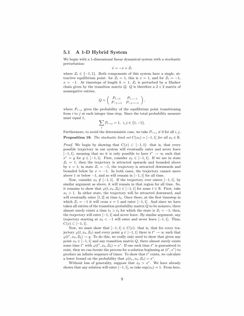
We can study the behavior of this system numerically. Figure 1 (left)depicts a solution calculated for the transition matrix

Q1 =

(.4 .6.5 .5

)with initial values x0 = 2, Z0 = 1.

As expected, the trajectory enters the interval (−1, 1) and stays therefor all time, oscillating between x = −1 and x = 1. Intuitively, it seemsthat the trajectory will cross any x∗ in this interval repeatedly, so thatindeed C(x) = [−1, 1]. This is not quite so clear for the transition matrix

Q2 =

(.1 .9.1 .9

)which yields the trajectory shown in Figure 1 (right) for x0 = 2, Z0 = 1.

It may appear that some set of points near x = 1 might be crossed byour path only a finite number of times. But, as proven above, any pointin (−1, 1) will almost surely be reached infinitely many times as t → ∞,so C(x) = [−1, 1].

Now, we consider the eigenvalues and eigenvectors of the transitionmatrices. The eigenvector of QT1 with eigenvalue 1 is

~v =

(511611

),

10

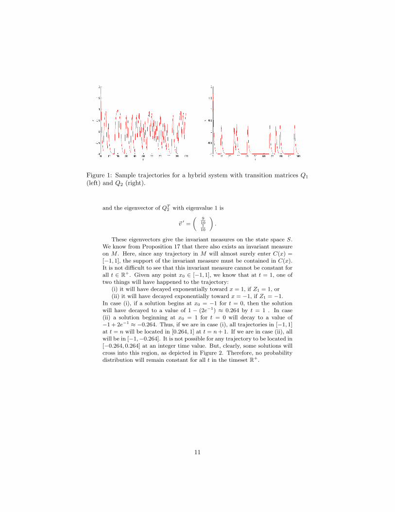
Figure 1: Sample trajectories for a hybrid system with transition matrices Q1

(left) and Q2 (right).

and the eigenvector of QT2 with eigenvalue 1 is

~v ′ =

(910110

).

These eigenvectors give the invariant measures on the state space S.We know from Proposition 17 that there also exists an invariant measureon M . Here, since any trajectory in M will almost surely enter C(x) =[−1, 1], the support of the invariant measure must be contained in C(x).It is not difficult to see that this invariant measure cannot be constant forall t ∈ R+. Given any point x0 ∈ [−1, 1], we know that at t = 1, one oftwo things will have happened to the trajectory:

(i) it will have decayed exponentially toward x = 1, if Z1 = 1, or(ii) it will have decayed exponentially toward x = −1, if Z1 = −1.

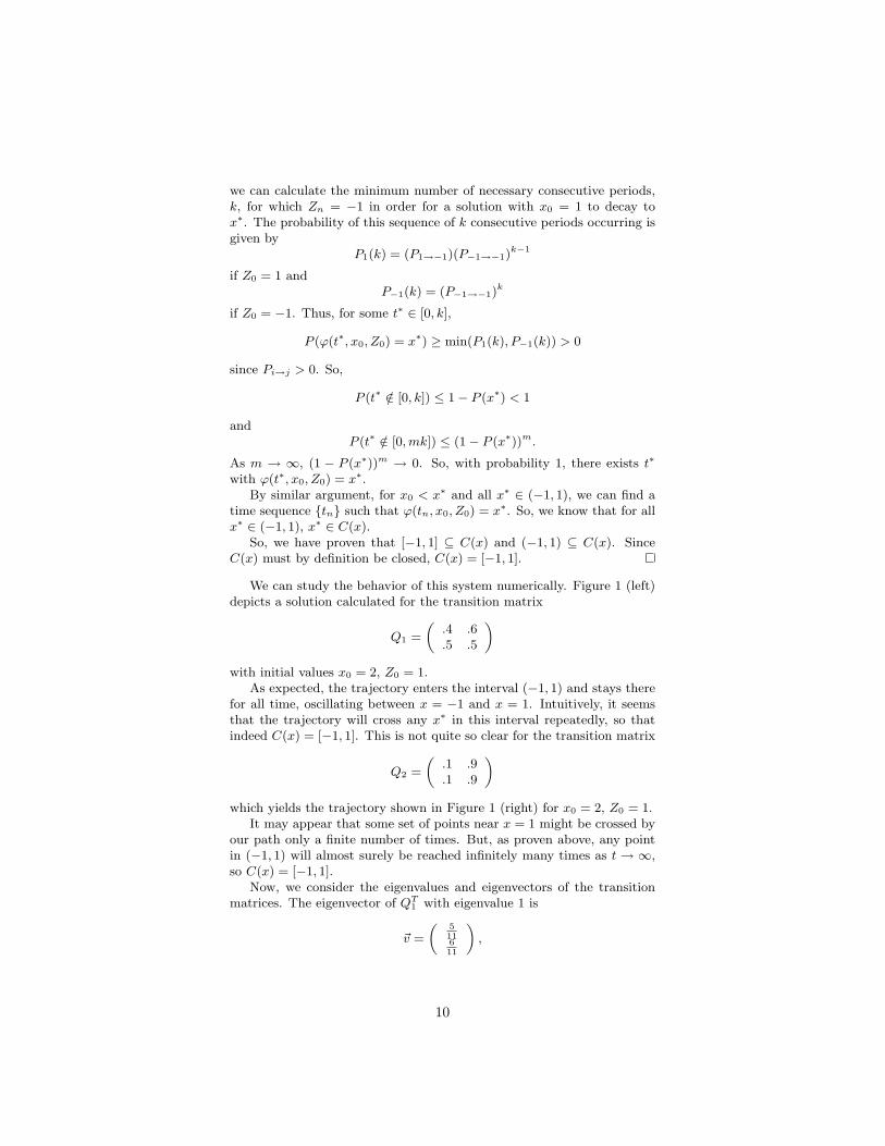
In case (i), if a solution begins at x0 = −1 for t = 0, then the solutionwill have decayed to a value of 1 − (2e−1) ≈ 0.264 by t = 1 . In case(ii) a solution beginning at x0 = 1 for t = 0 will decay to a value of−1 + 2e−1 ≈ −0.264. Thus, if we are in case (i), all trajectories in [−1, 1]at t = n will be located in [0.264, 1] at t = n+ 1. If we are in case (ii), allwill be in [−1,−0.264]. It is not possible for any trajectory to be located in[−0.264, 0.264] at an integer time value. But, clearly, some solutions willcross into this region, as depicted in Figure 2. Therefore, no probabilitydistribution will remain constant for all t in the timeset R+.

11

Figure 2: A spider plot showing all possible trajectories starting at x0 = 0.

However, as Figure 2 suggests, there is some distribution that is invari-ant under t→ t+ n for n ∈ N. Approximations of the invariant measuresat t ∈ [0, 1] for transition matrix Q1 are shown in Figure 3.

Figure 3: The invariant measure µ0 for a hybrid system with transition matrixQ1.

12

5.2 A 2-D Hybrid System

Our second example is a two-dimensional system used to model the ki-netics of chemical reactors. The general system f(x1, x2) is given by

x1 = −λx1 − β(x1 − xc) +BDaf(x1, x2)

x2 = −λx2 +Daf(x1, x2).

[5]Here, we use the following simplified application of the system:

x1 = −x1 − .15(x1 − 1) + .35(1− x2)ex1 + Zt(1− x1)

x2 = −x2 + .05(1− x2)ex1 .

This system is used to describe a Continuous Stirred Tank Reactor (CSTR).This type of reactor is used to control chemical reactions that require acontinuous flow of reactants and products and are easy to control thetemperature with. They are also useful for reactions that require workingwith two phases of chemicals.

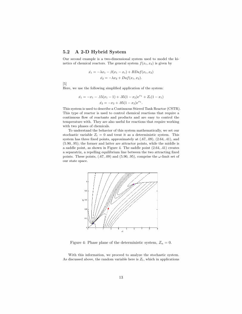
To understand the behavior of this system mathematically, we set ourstochastic variable Zt = 0 and treat it as a deterministic system. Thissystem has three fixed points, approximately at (.67, .09), (2.64, .41), and(5.90, .95); the former and latter are attractor points, while the middle isa saddle point, as shown in Figure 4. The saddle point (2.64, .41) createsa separatrix, a repelling equilibrium line between the two attracting fixedpoints. These points, (.67, .09) and (5.90, .95), comprise the ω-limit set ofour state space.

Figure 4: Phase plane of the deterministic system, Zn = 0.

With this information, we proceed to analyze the stochastic system.As discussed above, the random variable here is Zt, which in applications

13

can take values between −.15 and .15. To understand the full variabilityof this system, we take

Zt ∈ {−.15, 0, .15}

with the transition matrix .3 .3 .4.3 .3 .4.3 .3 .4

,

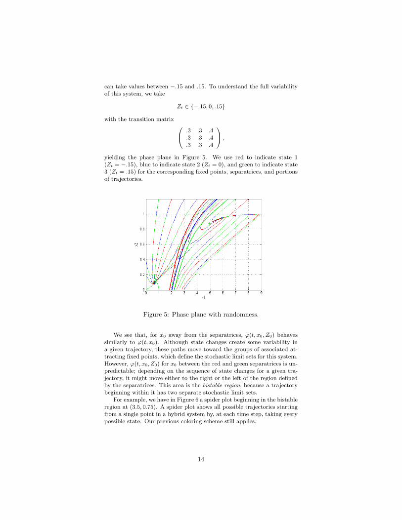
yielding the phase plane in Figure 5. We use red to indicate state 1(Zt = −.15), blue to indicate state 2 (Zt = 0), and green to indicate state3 (Zt = .15) for the corresponding fixed points, separatrices, and portionsof trajectories.

Figure 5: Phase plane with randomness.

We see that, for x0 away from the separatrices, ϕ(t, x0, Z0) behavessimilarly to ϕ(t, x0). Although state changes create some variability ina given trajectory, these paths move toward the groups of associated at-tracting fixed points, which define the stochastic limit sets for this system.However, ϕ(t, x0, Z0) for x0 between the red and green separatrices is un-predictable; depending on the sequence of state changes for a given tra-jectory, it might move either to the right or the left of the region definedby the separatrices. This area is the bistable region, because a trajectorybeginning within it has two separate stochastic limit sets.

For example, we have in Figure 6 a spider plot beginning in the bistableregion at (3.5, 0.75). A spider plot shows all possible trajectories startingfrom a single point in a hybrid system by, at each time step, taking everypossible state. Our previous coloring scheme still applies.

14

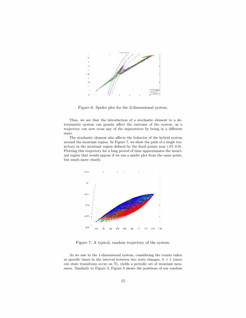
Figure 6: Spider plot for the 2-dimensional system.

Thus, we see that the introduction of a stochastic element to a de-terministic system can grossly affect the outcome of the system, as atrajectory can now cross any of the separatrices by being in a differentstate.

The stochastic element also affects the behavior of the hybrid systemaround the invariant region. In Figure 7, we show the path of a single tra-jectory in the invariant region defined by the fixed points near (.67, 0.9).Plotting this trajectory for a long period of time approximates the invari-ant region that would appear if we ran a spider plot from the same point,but much more clearly.

Figure 7: A typical, random trajectory of the system.

As we saw in the 1-dimensional system, considering the counts takenat specific times in the interval between two state changes, h = 1 (sinceour state transitions occur on N), yields a periodic set of invariant mea-sures. Similarly to Figure 3, Figure 8 shows the positions of our random

15

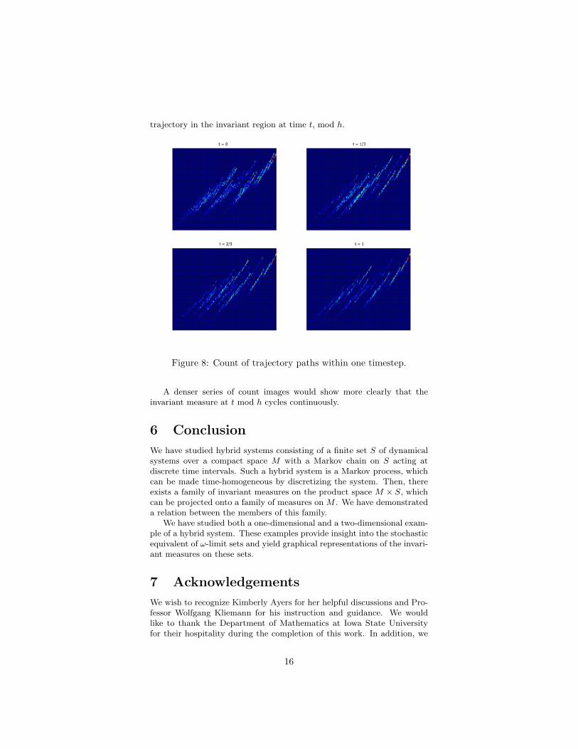
trajectory in the invariant region at time t, mod h.

Figure 8: Count of trajectory paths within one timestep.

A denser series of count images would show more clearly that theinvariant measure at t mod h cycles continuously.

6 Conclusion

We have studied hybrid systems consisting of a finite set S of dynamicalsystems over a compact space M with a Markov chain on S acting atdiscrete time intervals. Such a hybrid system is a Markov process, whichcan be made time-homogeneous by discretizing the system. Then, thereexists a family of invariant measures on the product space M × S, whichcan be projected onto a family of measures on M . We have demonstrateda relation between the members of this family.

We have studied both a one-dimensional and a two-dimensional exam-ple of a hybrid system. These examples provide insight into the stochasticequivalent of ω-limit sets and yield graphical representations of the invari-ant measures on these sets.

7 Acknowledgements

We wish to recognize Kimberly Ayers for her helpful discussions and Pro-fessor Wolfgang Kliemann for his instruction and guidance. We wouldlike to thank the Department of Mathematics at Iowa State Universityfor their hospitality during the completion of this work. In addition, we

16

would like to thank Iowa State University, Alliance, and the NationalScience Foundation for their support of this research.

References

[1] Ayers, K.D. Stochastic Perturbations of the Fitzhugh-Nagurno Equa-tions. Bowdoin College, Maine, 2010.

[2] Baldwin, M.C. Stochastic Analysis of Marotzke and Stone climatemodel. Iowa State University, Ames, 2007.

[3] Hairer, M. Convergence of Markov Processes. University of Warwick,Coventry, UK, 2010.

[4] Hairer, M. Ergodic Properties of Markov Processes. University of War-wick, Coventry, UK, 2006.

[5] Poore, A. B. A Model Equation Arising from Chemical Reactor The-ory. Arch. Rational Mech. Anal. 52 (1974), pp 358-388.

17