inventory management - massachusetts institute of...
TRANSCRIPT
Inventory Management Material Requirements Planning
Caplice
Lecture 10ESD.260 Fall 2003
© Chris Caplice, MIT2MIT Center for Transportation & Logistics – ESD.260
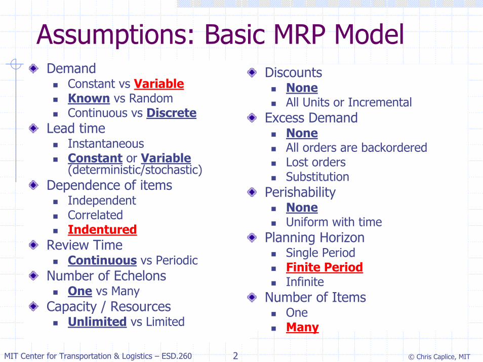
Assumptions: Basic MRP ModelDemand
Constant vs VariableKnown vs RandomContinuous vs Discrete
Lead timeInstantaneous Constant or Variable(deterministic/stochastic)
Dependence of itemsIndependentCorrelatedIndentured
Review TimeContinuous vs Periodic
Number of EchelonsOne vs Many
Capacity / ResourcesUnlimited vs Limited
DiscountsNoneAll Units or Incremental
Excess DemandNoneAll orders are backorderedLost ordersSubstitution
PerishabilityNoneUniform with time
Planning HorizonSingle PeriodFinite PeriodInfinite
Number of ItemsOneMany
© Chris Caplice, MIT3MIT Center for Transportation & Logistics – ESD.260
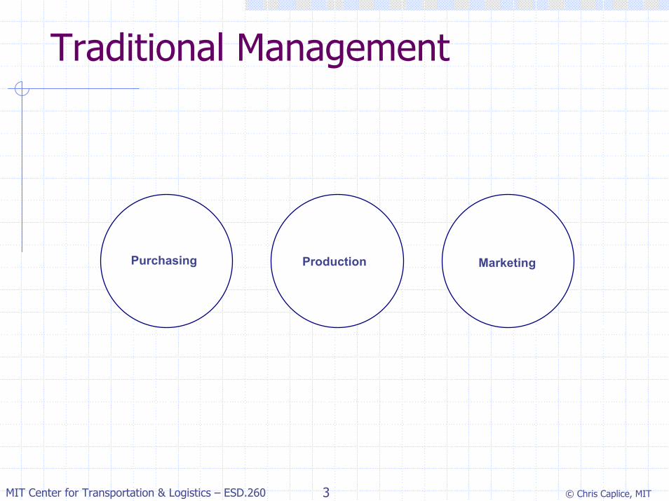
Traditional Management
Purchasing Production Marketing
© Chris Caplice, MIT4MIT Center for Transportation & Logistics – ESD.260
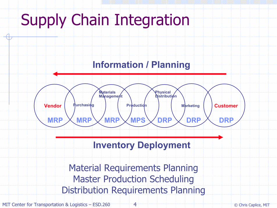
Supply Chain Integration
Information / Planning
Purchasing Production Marketing
MaterialsManagement
PhysicalDistribution
Vendor Customer
MRP DRPMPSMRP MRP DRPDRP
Inventory Deployment
Material Requirements PlanningMaster Production Scheduling
Distribution Requirements Planning
© Chris Caplice, MIT5MIT Center for Transportation & Logistics – ESD.260
Inventory Management so far . . .
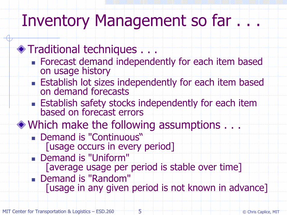
Traditional techniques . . . Forecast demand independently for each item based on usage historyEstablish lot sizes independently for each item based on demand forecastsEstablish safety stocks independently for each item based on forecast errors
Which make the following assumptions . . .Demand is "Continuous“ [usage occurs in every period]
Demand is "Uniform"[average usage per period is stable over time]
Demand is "Random"[usage in any given period is not known in advance]
© Chris Caplice, MIT6MIT Center for Transportation & Logistics – ESD.260
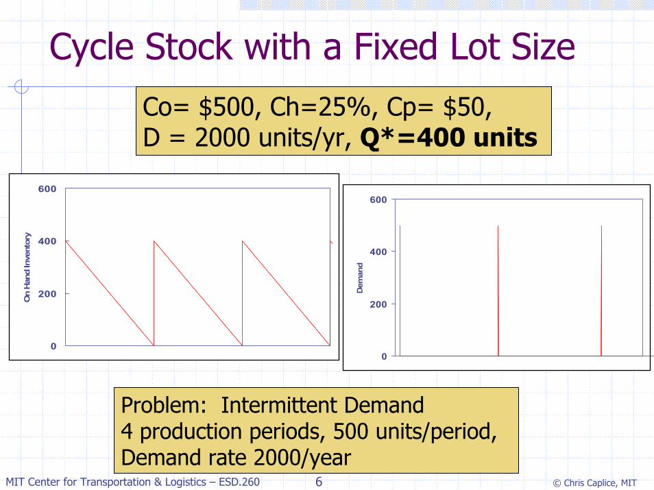
Cycle Stock with a Fixed Lot Size
0
200
400
600
On
Han
d In
vent
ory
Co= $500, Ch=25%, Cp= $50, D = 2000 units/yr, Q*=400 units
0
200
400
600
Dem
and
Problem: Intermittent Demand4 production periods, 500 units/period,Demand rate 2000/year
© Chris Caplice, MIT7MIT Center for Transportation & Logistics – ESD.260
0
200
400
600O
n H
and
Inve
ntor
y
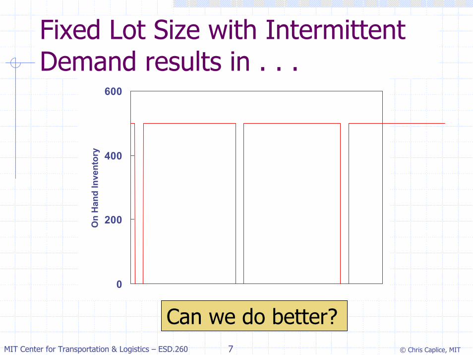
Fixed Lot Size with Intermittent Demand results in . . .
Can we do better?
© Chris Caplice, MIT8MIT Center for Transportation & Logistics – ESD.260
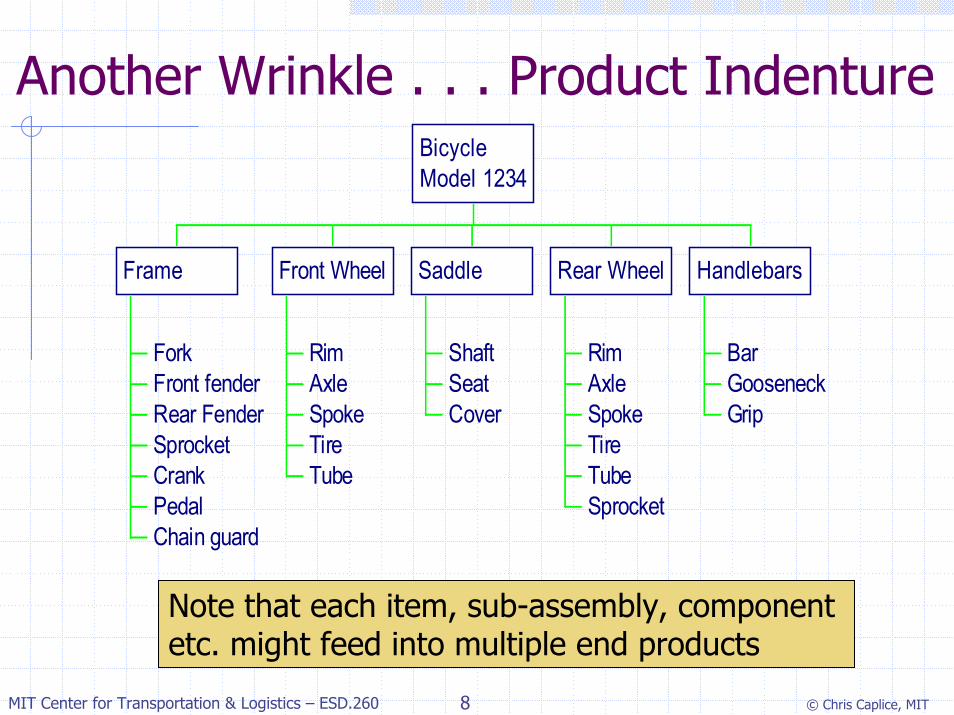
ForkFront fenderRear FenderSprocketCrankPedalChain guard
Frame
RimAxleSpokeTireTube
Front Wheel
ShaftSeatCover
Saddle
RimAxleSpokeTireTubeSprocket
Rear Wheel
BarGooseneckGrip
Handlebars
BicycleModel 1234
Another Wrinkle . . . Product Indenture
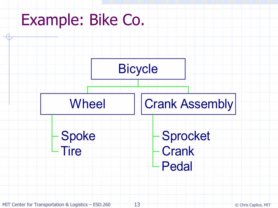
Note that each item, sub-assembly, component etc. might feed into multiple end products
© Chris Caplice, MIT9MIT Center for Transportation & Logistics – ESD.260
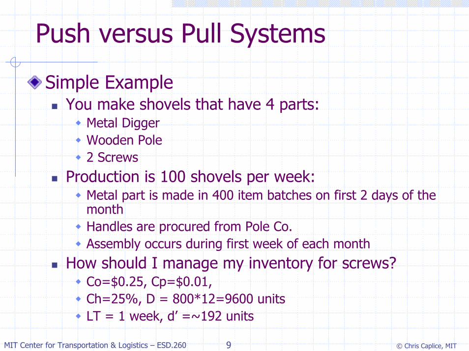
Push versus Pull Systems
Simple ExampleYou make shovels that have 4 parts:
Metal DiggerWooden Pole2 Screws
Production is 100 shovels per week:Metal part is made in 400 item batches on first 2 days of the monthHandles are procured from Pole Co. Assembly occurs during first week of each month
How should I manage my inventory for screws? Co=$0.25, Cp=$0.01, Ch=25%, D = 800*12=9600 unitsLT = 1 week, d’ =~192 units
© Chris Caplice, MIT10MIT Center for Transportation & Logistics – ESD.260
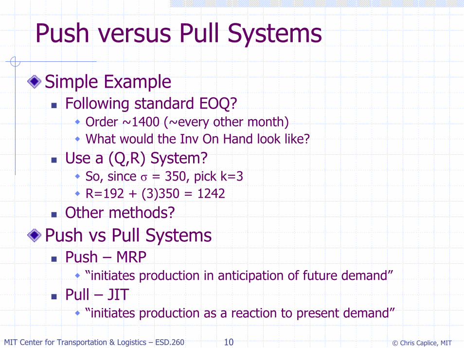
Push versus Pull Systems
Simple ExampleFollowing standard EOQ?
Order ~1400 (~every other month)What would the Inv On Hand look like?
Use a (Q,R) System?So, since σ = 350, pick k=3R=192 + (3)350 = 1242
Other methods?Push vs Pull Systems
Push – MRP“initiates production in anticipation of future demand”
Pull – JIT“initiates production as a reaction to present demand”
© Chris Caplice, MIT11MIT Center for Transportation & Logistics – ESD.260
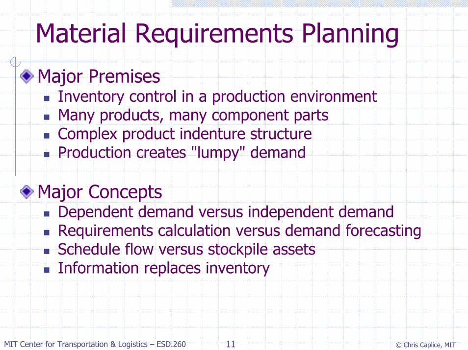
Material Requirements PlanningMajor Premises
Inventory control in a production environmentMany products, many component partsComplex product indenture structureProduction creates "lumpy" demand
Major ConceptsDependent demand versus independent demandRequirements calculation versus demand forecastingSchedule flow versus stockpile assetsInformation replaces inventory
© Chris Caplice, MIT12MIT Center for Transportation & Logistics – ESD.260
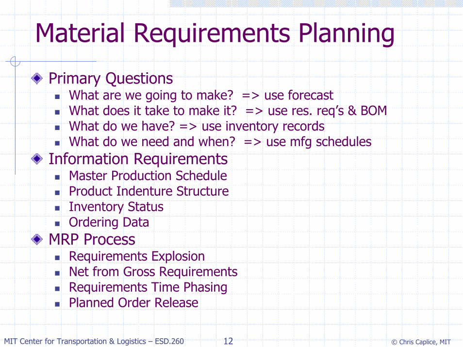
Material Requirements Planning
Primary QuestionsWhat are we going to make? => use forecastWhat does it take to make it? => use res. req’s & BOMWhat do we have? => use inventory recordsWhat do we need and when? => use mfg schedules
Information RequirementsMaster Production ScheduleProduct Indenture StructureInventory StatusOrdering Data
MRP ProcessRequirements ExplosionNet from Gross RequirementsRequirements Time PhasingPlanned Order Release
© Chris Caplice, MIT13MIT Center for Transportation & Logistics – ESD.260
Example: Bike Co.
SpokeTire
Wheel
SprocketCrankPedal
Crank Assembly
Bicycle
© Chris Caplice, MIT14MIT Center for Transportation & Logistics – ESD.260
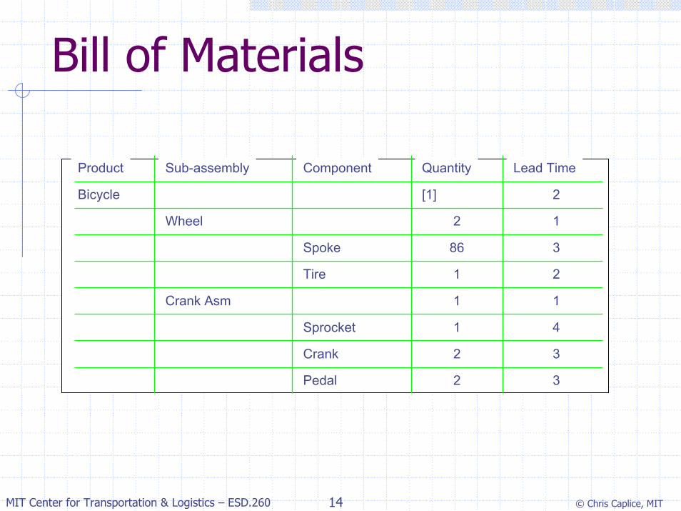
Bill of Materials
Product Sub-assembly Component Quantity Lead Time
Bicycle [1] 2
Wheel 2 1
Spoke 86 3
Tire 1 2
Crank Asm 1 1
Sprocket 1 4
Crank 2 3
Pedal 2 3
© Chris Caplice, MIT15MIT Center for Transportation & Logistics – ESD.260
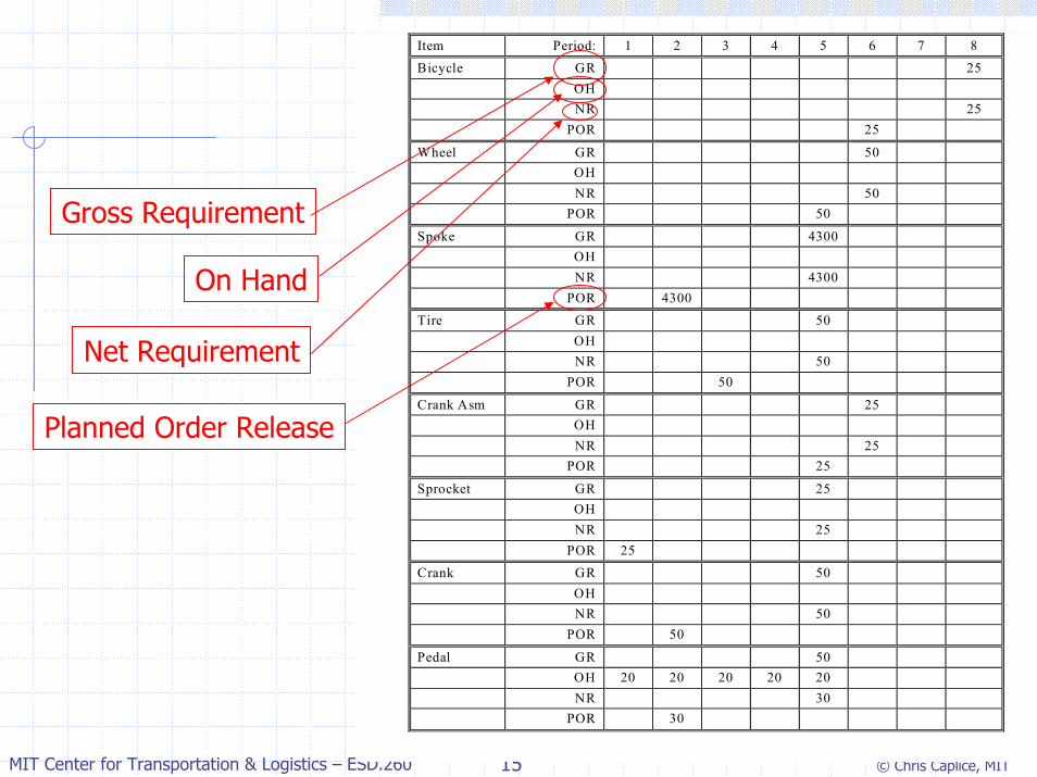
Item Period: 1 2 3 4 5 6 7 8 Bicycle GR 25 OH NR 25 POR 25
Wheel GR 50 OH NR 50 POR 50
Spoke GR 4300 OH NR 4300 POR 4300 Tire GR 50 OH NR 50 POR 50
Crank Asm GR 25 OH NR 25 POR 25
Sprocket GR 25 OH NR 25 POR 25 Crank GR 50 OH NR 50 POR 50
Pedal GR 50 OH 20 20 20 20 20 NR 30 POR 30
Gross Requirement
On Hand
Net Requirement
Planned Order Release
© Chris Caplice, MIT16MIT Center for Transportation & Logistics – ESD.260
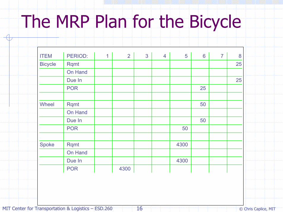
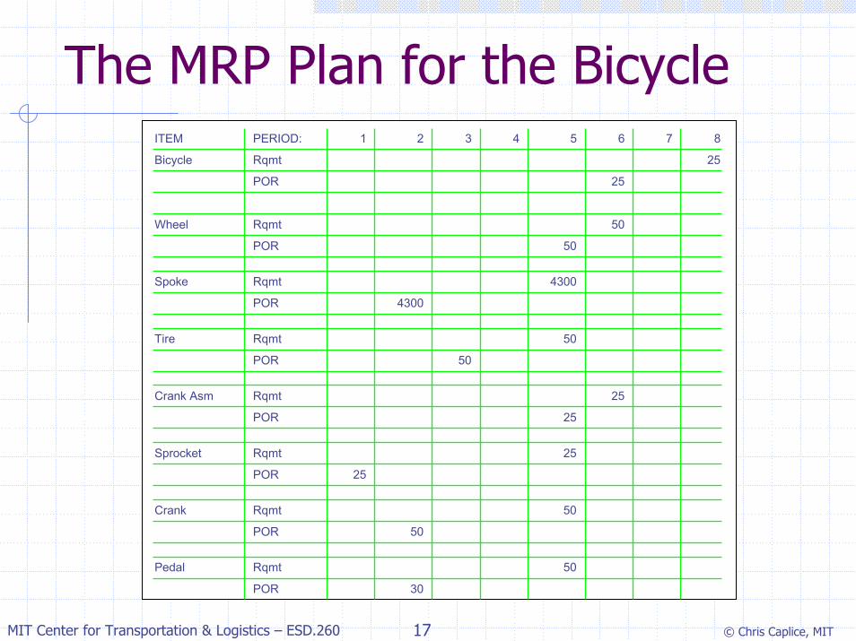
The MRP Plan for the Bicycle
ITEM PERIOD: 1 2 3 4 5 6 7 8Bicycle Rqmt 25
On HandDue In 25POR 25
>> >> >> >> >> >> >> >>Wheel Rqmt 50
On HandDue In 50POR 50
>Spoke Rqmt 4300
On HandDue In 4300POR 4300
© Chris Caplice, MIT17MIT Center for Transportation & Logistics – ESD.260
The MRP Plan for the BicycleITEM PERIOD: 1 2 3 4 5 6 7 8
Bicycle Rqmt 25
POR 25
>> >> >> >> >> >> >> >>
Wheel Rqmt 50
POR 50
Spoke Rqmt 4300
POR 4300
Tire Rqmt 50
POR 50
Crank Asm Rqmt 25
POR 25
Sprocket Rqmt 25
POR 25
Crank Rqmt 50
POR 50
Pedal Rqmt 50
POR 30
© Chris Caplice, MIT18MIT Center for Transportation & Logistics – ESD.260
Two Issues
How do we handle capacity constraints?
How do we handle uncertainty?Safety Stock
Add to existing stockWhere would this be applied?
Safety TimesPad the planned lead timesWhere would this be applied?
© Chris Caplice, MIT19MIT Center for Transportation & Logistics – ESD.260
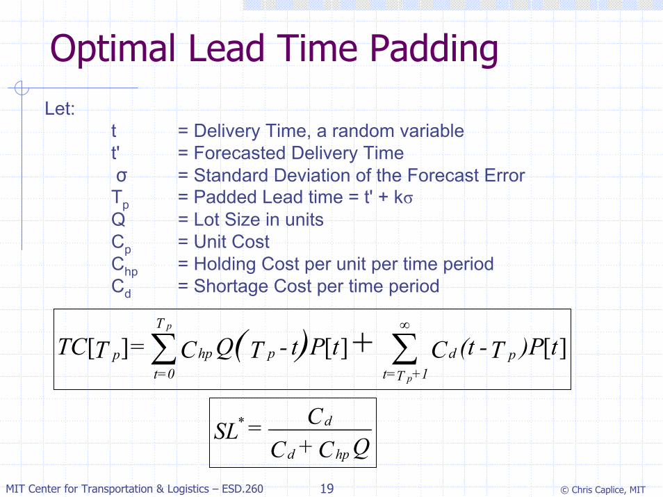
Optimal Lead Time PaddingLet:
t = Delivery Time, a random variablet' = Forecasted Delivery Timeσ = Standard Deviation of the Forecast ErrorTp = Padded Lead time = t' + kσQ = Lot Size in unitsCp = Unit CostChp = Holding Cost per unit per time periodCd = Shortage Cost per time period
][][][ t)PT-(tCtPt-TQC = TTC pd1+T=t
php
T
=0tp
p
p
+ )( ∑∑∞
QC + CC = SL
hpd
d*
© Chris Caplice, MIT20MIT Center for Transportation & Logistics – ESD.260
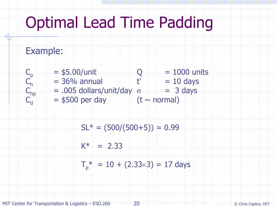
Optimal Lead Time Padding
Example:
Cp = $5.00/unit Q = 1000 unitsCh = 36% annual t' = 10 daysChp = .005 dollars/unit/day σ = 3 daysCd = $500 per day (t ~ normal)
SL* = (500/(500+5)) = 0.99
K* = 2.33
Tp* = 10 + (2.33×3) = 17 days
© Chris Caplice, MIT21MIT Center for Transportation & Logistics – ESD.260
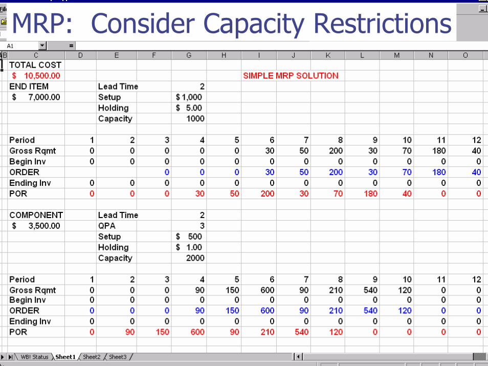
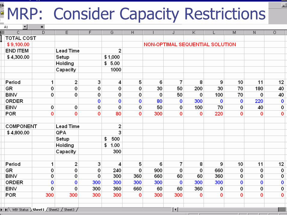
MRP: Consider Capacity Restrictions
© Chris Caplice, MIT22MIT Center for Transportation & Logistics – ESD.260
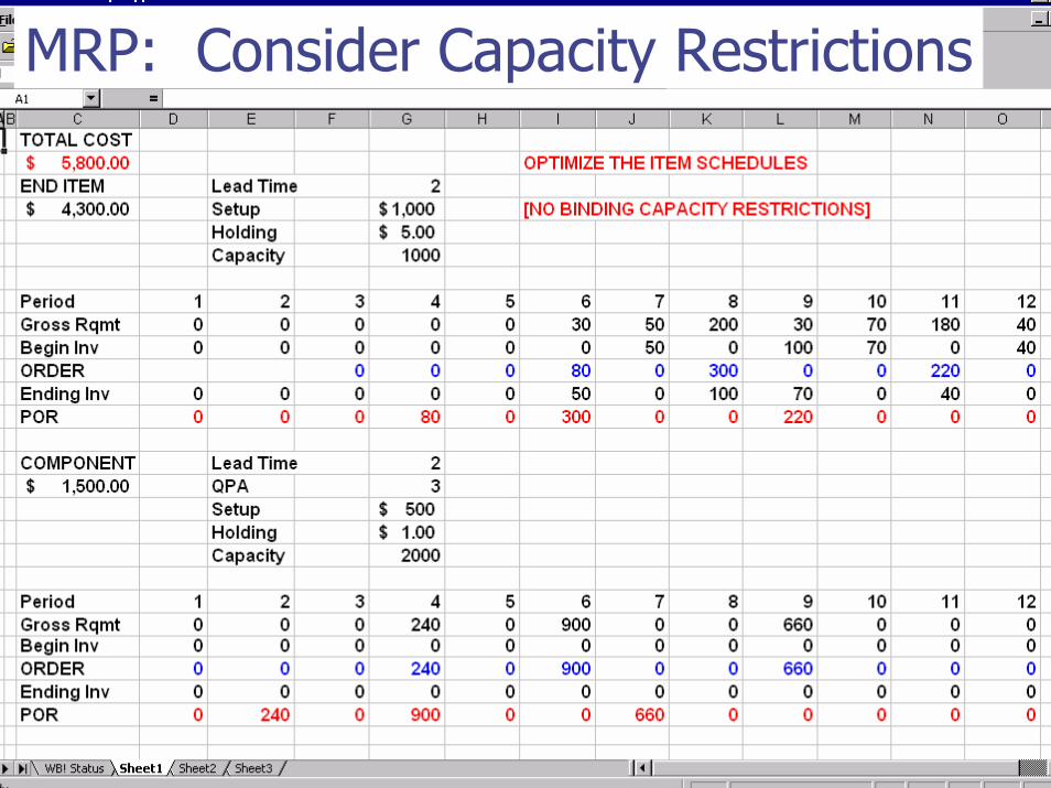
MRP: Consider Capacity Restrictions
© Chris Caplice, MIT23MIT Center for Transportation & Logistics – ESD.260
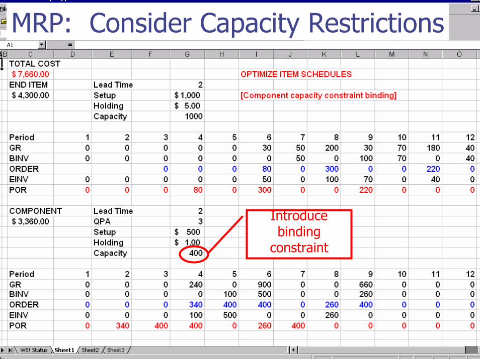
Introduce binding
constraint
MRP: Consider Capacity Restrictions
© Chris Caplice, MIT24MIT Center for Transportation & Logistics – ESD.260
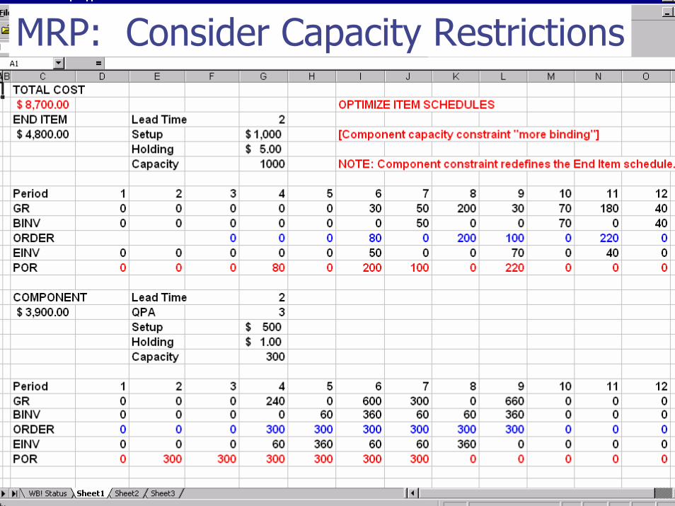
MRP: Consider Capacity Restrictions
© Chris Caplice, MIT25MIT Center for Transportation & Logistics – ESD.260
MRP: Consider Capacity Restrictions
© Chris Caplice, MIT26MIT Center for Transportation & Logistics – ESD.260
Benefits of MRP
Lower Inventory LevelsAble to better manage components Increased visibility
Fewer Stock outsRelationships are defined and explicitAllows for coordination with MPS
Less ExpeditingDue to increased visibility
Fewer Production DisruptionsInput needs are explicitly modeledPlans are integrated
© Chris Caplice, MIT27MIT Center for Transportation & Logistics – ESD.260
Shortcomings of MRPMRP is a scheduling, not a stockage, algorithm
Replaces the forecasting mechanismConsiders indentured structures
MRP does not address how to determine lot sizeDoes not explicitly consider costsWide use of Lot for Lot in practice
MRP systems do not inherently deal with uncertaintyUser must enter these values – by item by production levelTypical use of "safety time“ rather than "safety stock“
MRP assumes constant, known leadtimesBy component and part and production levelBut lead time is often a function of order size and other activity
MRP does not provide incentives for improvementRequires tremendous amount of data and effort to set upInitial values are typically inflated to avoid start up issuesLittle incentive to correct a system “that works”
© Chris Caplice, MIT28MIT Center for Transportation & Logistics – ESD.260
MRP: Evolution of Concepts
Simple MRPFocus on "order launching“Used within production – not believed outside
Closed Loop MRPFocus on production schedulingInteracts with the MPS to create feasible plans
MRP II [Manufacturing Resource Planning]Focus on integrated financial planningTreats the MPS as a decision variableCapacity is considered (Capacity Resource Planning)
Enterprise Resource Planning SystemsCommon, centralized data for all areasImplementation is costly and effort intensiveForces business rules on companies