Ann Oper Res (2010) 176: 7–39DOI 10.1007/s10479-009-0513-8

Inventory management with partially observednonstationary demand

Erhan Bayraktar · Michael Ludkovski

Published online: 29 January 2009© Springer Science+Business Media, LLC 2009

Abstract We consider a continuous-time model for inventory management with Markovmodulated non-stationary demands. We introduce active learning by assuming that the stateof the world is unobserved and must be inferred by the manager. We also assume that de-mands are observed only when they are completely met. We first derive the explicit filteringequations and pass to an equivalent fully observed impulse control problem in terms of thesufficient statistics, the a posteriori probability process and the current inventory level. Wethen solve this equivalent formulation and directly characterize an optimal inventory policy.We also describe a computational procedure to calculate the value function and the optimalpolicy and present two numerical illustrations.

Keywords Inventory management · Markov modulated Poisson process · Hidden Markovmodel · Partially observable demand · Censored demand

1 Introduction

Inventory management aims to control the supply ordering of a firm so that inventory costsare minimized and a maximum of customer orders are filled. These are competing objectivessince low inventory stock reduces storage and ordering costs, whereas high inventory avoidsstock-outs. The problem is complicated by the fact that real-life demand is never station-ary and therefore the inventory policy should be non-stationary as well. A popular methodof addressing this issue is to introduce a regime-switching (or Markov-modulated) demand

E. Bayraktar is supported in part by the National Science Foundation.

E. Bayraktar (!)Department of Mathematics, University of Michigan, Ann Arbor, MI 48109, USAe-mail: erhan@umich.edu

M. LudkovskiDepartment of Statistics and Applied Probability, University of California Santa Barbara,Santa Barbara, CA 93106-3110, USAe-mail: ludkovski@pstat.ucsb.edu

8 Ann Oper Res (2010) 176: 7–39

model. The regime is meant to represent the economic environment faced by the firm anddrives the parameters (frequency and size distribution) of the actual demand process. How-ever, typically this economic environment is unknown. From a modeling perspective, thisleads to a partially observed hidden Markov model for demand. Thus, the inventory managermust simultaneously learn the current environment (based on incoming order information),and adjust her inventory policy accordingly in anticipation of future orders.

The literature on inventory management with non-stationary Markovian demand orig-inated with Song and Zipkin (1993) who considered a continuous-time model where thedemand levels or intensity are modulated by the state of the world, which are assumed tobe observable. The discrete-time counterpart of this model was then analyzed by Sethi andCheng (1997) who allowed a very general cost structure and proved a more formal verifica-tion theorem for existence and regularity of the value function and existence of an optimalfeedback policy. More recent work on fully observed non-stationary demand can be foundin Bensoussan et al. (2005b).

Inventory management with partial information is a classical topic of operations re-search. In the simplest version as analyzed by Azoury (1985), Lovejoy (1990) and refer-ences therein, the demand distribution is unknown and must be learned by the controller.Thus, a finite-horizon discrete time parameter adaptive model is considered, so that the de-mand distribution is taken to be stationary and i.i.d., but with an unknown parameter. Thisparameter is then inferred over time using either an exponential smoothing or a Bayesianlearning mechanism. In these papers the method of solution relied on the special structureof some particular cases (e.g. uniform demand level on [0,w], with w unknown) where adimension reduction is possible, so that the learning update is simplified. Even after that, theproblem remains extremely computationally challenging; accordingly the focus of Lovejoy(1990) has been on studying approximate myopic or limited look-ahead policies.

Another important strand of literature investigates the lost sales uncertainty. In that case,demand is observed only if it is completely met; instead of a back-order, unmet demandis lost. This then creates a partial information problem if demand levels are non-stationary.In particular, demand levels evolving according to a discrete-time Markov chain have beenconsidered in the newsvendor context (completely perishable inventory) by Lariviere andPorteus (1999), Beyer and Sethi (2005), Bensoussan et al. (2007a), and in the general inven-tory management case by Bensoussan et al. (2008). Bensoussan et al. (2005a, 2007b) haveanalyzed the related case whereby current inventory level itself is uncertain.

The main inspiration for our model is the work of Treharne and Sox (2002) who consid-ered a version of the Sethi and Cheng (1997) model but under the assumption that currentworld state is unknown. The controller must therefore filter the present demand distribu-tion to obtain information on the core process. Treharne and Sox (2002) take a partiallyobserved Markov decision processes (POMDP) formulation; since this is computationallychallenging, they focus on empirical study of approximate schemes, in particular myopicand limited look-ahead learning policies, as well as open-loop feedback learning. A relatedproblem of dynamic pricing with unobserved Markov-modulated demand levels has beenrecently considered by Aviv and Pazgal (2005). In that paper, the authors also work in thePOMDP framework and propose a different approximation scheme based on the techniqueof information structure modification.

In this paper we consider a continuous-time model for inventory management withMarkov modulated non-stationary demands. We take the Song and Zipkin (1993) model asthe starting point and introduce active learning by assuming that the state of the core processis unobserved and must be inferred by the controller. We will also assume that the demand isobserved only when it is completely met, otherwise censoring occurs. Our work extends the

Ann Oper Res (2010) 176: 7–39 9

results of Bensoussan et al. (2007a, 2008) and Treharne and Sox (2002) to the continuous-review asynchronous setting. Use of continuous- rather than discrete-time model facilitatessome of our analysis. It is also more realistic in medium-volume problems with many asyn-chronous orders (e.g. computer hardware parts, industrial commodities, etc.), especially inapplications with strong business cycles where demand distribution is highly non-stationary.In a continuous-time model, the controller may adjust inventory immediately after a neworder, but also between orders. This is because the controller’s beliefs about the demand en-vironment are constantly evolving. Such qualitative distinction is not possible with discreteepochs where controls and demand observations are intrinsically paired.

Our method of solution consists of two stages. In the first stage (Sect. 2), we derive ex-plicit filtering equations for the evolution of the conditional distribution of the core process.This is non-trivial in our model where censoring links the observed demand process with thechosen control strategy. We use the theory of partially observed point processes to extendearlier results of Arjas et al. (1992), Ludkovski and Sezer (2007), Bayraktar and Ludkovski(2008) in Proposition 2.1. The piecewise deterministic strong Markov process obtained inProposition 2.1 allows us then to give a simplified and complete proof of the dynamic pro-gramming equations, and describe an optimal policy (see Sect. 3). We achieve this by lever-aging the general probabilistic arguments for the impulse control of piecewise deterministicprocesses of Davis (1993), Costa and Davis (1989), Gatarek (1992) and using direct argu-ments to establish necessary properties of the value function. Our approach is in contrastwith the POMDP and quasi-variational formulations in the aforementioned literature thatmake use of more analytic tools.

Our framework also leads to a different flavor for the numerical algorithm. The closed-form formulas obtained in Sects. 2 and 3 permit us to give a direct and simple-to-implementcomputational scheme that yields a precise solution. Thus, we do not employ any of the ap-proximate policies proposed in the literature, while maintaining a competitive computationalcomplexity.

To summarize, our contribution is a full and integrated analysis of such incompleteinformation setting, including derivation of the filtering equations, characterization of anoptimal policy and a computationally efficient numerical algorithm. Our results show thefeasibility of using continuous-time partially observed models in inventory managementproblems. Moreover, our model allows for many custom formulations, including arbitraryordering/storage/stock-out/salvage cost structures, different censoring formulations, perish-able inventory and supply-size constraints.

The rest of the paper is organized as follows. In the rest of the introduction we will givean informal description of the inventory management problem we are considering. In Sect. 2we make the formulation more precise and show that the original problem is equivalent to afully observed impulse control problem described in terms of sufficient statistics. Moreover,we characterize the evolution of the paths of the sufficient statistics. In Sect. 3 we showthat the value function is the unique fixed point of a functional operator (defined in termsof an optimal stopping problem) and that it is continuous in all of its variables. Using thecontinuity of the value function we describe an optimal policy in Sect. 3.2. In Sect. 3.3 wedescribe how to compute the value function using an alternative characterization. Finally,in Sect. 4 we present two numerical illustrations. Some of the longer proofs are left toAppendices A and B.

1.1 Model description

In this section we give an informal description of the inventory management with partialinformation and the objective of the controller. A rigorous construction is in Sect. 2.

10 Ann Oper Res (2010) 176: 7–39

Let M be the unobservable Markov core process for the economic environment. Weassume that M is a continuous-time Markov chain with finite state space E ! {1, . . . ,m}.The core process M modulates customer orders modeled as a compound Poisson process X.More precisely, let Y1, Y2, . . . be the consecutive order sizes, taking place at times !1,!2, . . . .

Define

N(t) = sup{s : !s < t} (1.1)

to be the number of orders received by time t , and

Xt =N(t)!

k=1

Yk, (1.2)

to be the total order size by time t . Then, the intensity of N (and X) is "i whenever M is atstate i, for i ! E. Similarly, the distribution of Yk is #i conditional on M!k

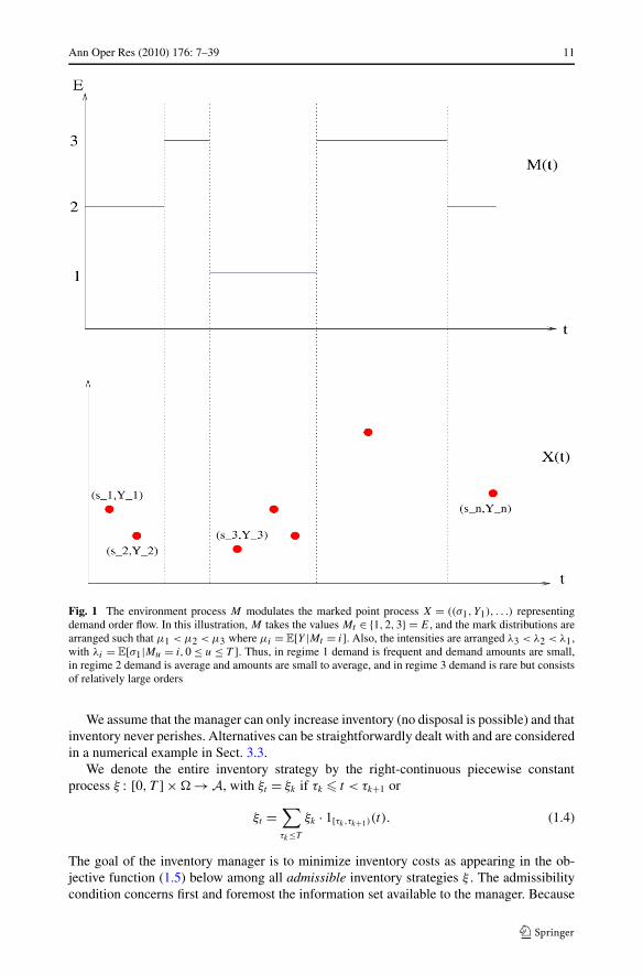
= i. This structureis illustrated schematically in Fig. 1. The assumption of demand following a compoundPoisson process is standard in the OR literature, especially when considering large items(the case of demand level following a jump-diffusion is investigated by Bensoussan et al.2005b).

We assume that orders are integer-sized with a fixed upper bound R, namely

Assumption Each #i , i ! E is a discrete bounded distribution on Z, so that Yk !{1,2, . . . ,R}.

The controller cannot observe M ; neither does she directly see X. Instead, she receivesthe censored order flow W . The order flow W consists of filled order amounts (Z$), whichinformally correspond to the minimum between actual order size and available inventory.Hence, if total inventory is insufficient, a stock-out occurs and the excess order size is leftindeterminate. The model where order flow is always observed will also be considered as aspecial case with zero censoring. The precise description of W will be given in Sect. 2.1.

Let Pt be the current inventory at time t . We assume that inventory has finite stock capac-ity, so that Pt ! [0,P ]. Inventory changes are driven by two variables: filled customer ordersdescribed by W and supply orders. Customer orders are assumed to be exogenous; everyorder is immediately filled to its maximum extent. When a stock-out occurs, we considertwo scenarios:

• If there is no censoring, then the excess order amount is immediately back-ordered at ahigher penalty rate.

• If there is censoring, a lost opportunity cost is assessed in proportion to expected excessorder amount.

Otherwise, the inventory is immediately decreased by the order amount. Supply orders arecompletely at the discretion of the manager. Let %1, %2, . . . denote the supply amounts (with-out back-orders) and &1, &2, . . . the supply times (when supply order is placed).

To summarize, the dynamics of P are (compare to (2.12) below):

"#

$

P!k= (P!k" " Zk), fill customer order

P&k = P&k" + %k, new supply orderdPt = 0 otherwise.

(1.3)

Ann Oper Res (2010) 176: 7–39 11

Fig. 1 The environment process M modulates the marked point process X = ((!1, Y1), . . .) representingdemand order flow. In this illustration, M takes the values Mt ! {1,2,3} = E, and the mark distributions arearranged such that µ1 < µ2 < µ3 where µi = E[Y |Mt = i]. Also, the intensities are arranged "3 < "2 < "1,with "i = E[!1|Mu = i,0 # u # T ]. Thus, in regime 1 demand is frequent and demand amounts are small,in regime 2 demand is average and amounts are small to average, and in regime 3 demand is rare but consistsof relatively large orders

We assume that the manager can only increase inventory (no disposal is possible) and thatinventory never perishes. Alternatives can be straightforwardly dealt with and are consideredin a numerical example in Sect. 3.3.

We denote the entire inventory strategy by the right-continuous piecewise constantprocess % : [0, T ] $ ' % A, with %t = %k if &k " t < &k+1 or

%t =!

&k#T

%k · 1[&k,&k+1)(t). (1.4)

The goal of the inventory manager is to minimize inventory costs as appearing in the ob-jective function (1.5) below among all admissible inventory strategies % . The admissibilitycondition concerns first and foremost the information set available to the manager. Because

12 Ann Oper Res (2010) 176: 7–39

Table 1 Parameters of themodel Parameter Meaning

c(a) Storage cost for a items per unit time

K(a) Instantaneous stock-out cost for a shortage of a items

h Order cost for one item

( Fixed cost of placing an order

) Discount factor for NPV calculation

P Maximum inventory size

R Maximum demand size

only W is observable, the strategy % should be determined by the information generated byW , namely each &k must be a stopping time of the filtration FW ! {F W

t } of W . Similarly, thevalue of each %k is determined by the information F W

&krevealed by W until &k . Also, without

loss of generality we assume that % has a finite number of actions, so that P(&k < T ) % 0as k % &. Since strategies with infinitely many actions will have infinite costs, we cansafely exclude them from consideration. We denote by U (T ) the set of all such admissiblestrategies on a time interval [0, T ].

The selected policy % directly influences current stocks P ; when we wish to emphasizethis dependence we will write Pt ' P

%t . The cost of implementing % is as follows. First,

inventory storage costs at fixed rate c(Pt ) are accessed. We assume that c is positive, in-creasing and continuous. Second, a supply order of size %k costs h · %k + ( , for positive h

and ( . Finally, if a stock-out occurs due to insufficient existing stock, a penalty reflecting thelost opportunity cost is assessed at amount E[K((Yk " P!k")+)|F W

t ]. We assume that thepenalty function K is positive and increasing with K(0) = 0. Thus, the total performance ofa strategy % on the horizon [0, T ] is

% T

0e")t c(Pt ) dt +

!

k:&k<T

e")&k (h · %k + ( ) +!

$:!$<T

e")!$K((Y$ " P!$")+), (1.5)

where ) ( 0 is the discount factor for future revenue. Table 1 summarizes our notation andthe meaning of the model parameters.

Observe that the objective in (1.5) involves the distribution of Zk’s (which affect P ) andYk’s (which enter into objective function through stock-out costs). Both of these depend onthe state M . Since the core process M is unobserved, the controller must therefore carryout a filtering procedure. We postulate that she collects information about M via a Bayesianframework. Let )* = (*1, . . . ,*m) ! (P{M0 = 1}, . . . ,P{M0 = m}) be the initial (prior) be-liefs of the controller about M and P)* the corresponding conditional probability law. Thecontroller starts with beliefs * , observes Z, updates her beliefs and adjusts her inventorypolicy accordingly.

These notions and the precise updating mechanism will be formalized in Sect. 2.4. Thesolution will then proceed in two steps: an initial filtering step and a second optimizationstep. The inference step is studied in Sect. 2, where we introduce the a posteriori probabilityprocess )+. The process )+ summarizes the dynamic updating of controller’s beliefs about theMarkov chain M given her point process observations. The optimal switching problem (2.5)is then analyzed in Sect. 3.

Ann Oper Res (2010) 176: 7–39 13

2 Problem statement

In this section we give a mathematically precise description of the problem and show thatthis problem is equivalent to a fully observed impulse control problem in terms of thestrong Markov process ( )+,P ). We will also describe the dynamics of the sufficient sta-tistics ( )+,P ).

2.1 Core process

Let (', H,P) be a probability space hosting two independent elements: (i) a continuoustime Markov process M taking values in a finite set E, and with infinitesimal generatorQ = (qij )i,j!E , (ii) X(1), . . . ,X(m) which are independent compound Poisson processes withintensities and discrete jump size distributions ("1,#1), . . . , ("m,#m), respectively, m ! E.

The core point process X is given by

Xt ! X0 +% t

0

!

i!E

1{Ms=i} dX(i)s , t ( 0. (2.1)

Thus, X is a Markov-modulated Poisson process (see e.g. Karlin and Taylor 1981); by con-struction, X has independent increments conditioned on M = {Mt }t(0. Denote by !0,!1, . . .

the arrival times of the process X,

!$ ! inf{t > !$"1 : Xt *= Xt"}, $ ( 1 with !0 ' 0.

and by Y1, Y2, . . . the R-valued marks (demand sizes) observed at these arrival times:

Y$ = X!$" X!$", $ ( 1.

Then conditioned on {M!$= i}, the distribution of Y$ is described by #i (dy) = fi(y)dy on

(Z+, B(Z+)).

2.2 Observation process

Starting with the marked point process (M,X), the observable is a point process W which isderived from (M,X). This means that the marks of W are completely determined by (M,X)

(and the control). Fix an initial stock P(1)0 = a. We first construct an auxiliary process W (1).

The first mark of W (1) is (!1,Z1), where !1 is the first arrival time of X and where thedistribution of the first jump size Z1 = (Z1

1,Z21) ! Z conditional on (M,X) given by

P(Z1 = )z|Y1 = y,M!1 = i) = C(y, )z; P (1)!1"),

where C(y, )z;a), y ! Z+, )z ! Z, a ! [0,P ] are the {0,1}-valued censoring functions satis-fying

&)z!Z C(y, )z;a) ! {0,1}. In our context, it is convenient to take Z = Z+ $ {0,,},

where )z ' (z1, z2) ! Z represents a filled order of size z1, and the second componentz2 indicates whether a stock-out occurred or not. Censoring of excess orders then corre-sponds to C(y, )z;p) = 1{(0,p]}(y)1{(y,0)}()z) + 1{(p,R)}(y)1{(+p,,,)}()z). Alternatively, withoutcensoring we take Z = Z+ $ Z+ (second component now indicating actual order size), andC(y, )z;p) = 1{(0,p]}(y)1{(y,y)}()z) + 1{(p,R]}(y)1{(+p,,y)}()z).

Once (!1,Z1) is observed, we update P (1)!1

= a"Z11 ( 0, and set P

(1)t = P (1)

!1for !1 # t <

!2, where !2 is the second arrival time of X. Proceeding as before, we will obtain the markedpoint process W (1) = (!$,Z$) and the corresponding uncontrolled stock process P (1).

14 Ann Oper Res (2010) 176: 7–39

We now introduce the first impulse control. Let {F W (1)

t } be the filtration generated byW (1), and let (&1, %1) be an F W (1)

-stopping time, and an F W (1)

&1-measurable Z+-valued ran-

dom variable, respectively, satisfying &1 # T ,0 # %1 # P " P(1)&1". The impulse control means

that we take W = W (1)1[0,&1), Pt = P(1)t 1[0,&1) and repeat the above construction on the inter-

val [&1, T ] starting with the updated value P (2)&1

= P(1)&1" + %1.

Inductively this provides the auxiliary point processes W (k) together with the im-pulse controls (&k, %k), k = 1,2, . . . . Letting % = (&1, %1, &2, %2, . . .) we finally obtain the% -controlled inventory process P , as well as the % -controlled marked point process W =&

k W (k)1[0,&k). By construction, both P and % are FW -measurable. We denote by Pa,% theresulting probability law of (W,P ).

Summarizing, P is a piecewise-deterministic controlled process taking values in [0,P ]and evolving as in (1.3); the arrival times of W are those of X, and the distribution of itsmarks (Z$) depends inductively on the latest P!$", the mark Y$ of core process X, and thecensoring functions c

pi (y, z). For further details of the above construction of Pa,% we refer

the reader to Davis (1993), pp. 228–230. Our use of censoring functions is similar to theconstruction in Arjas et al. (1992).

2.3 Statement of the objective function in terms of sufficient statistics

Let D ! {)* ! [0,1]m : *1 + · · · + *m = 1} be the space of prior distributions of theMarkov process M . Also, let S(s) = {& : F-stopping time, & # s,P-a.s} denote the set ofall F-stopping times smaller than or equal to s.

Let P)* ,a,% denote the probability measure Pa,% such that the process M has initial distri-bution )* . That is,

P)* ,a,% {A} = *1Pa,% {A|M0 = 1} + · · · + *mPa,% {A|M0 = m} (2.2)

for all A ! F WT . P)* can be similarly defined. In the sequel, when % ' 0, we will denote the

corresponding probability measure by P)* ,a

We define the D-valued conditional probability process )+(t) ! (+1(t), . . . ,+m(t)) suchthat

+i (t) = P)* ,a,% {Mt = i|F Wt }, for i ! E, and t ( 0. (2.3)

Each component of )+ gives the conditional probability that the current state of M is {i}given the information generated by W until the current time t .

Using )+ we convert the original objective (1.5) into the following F-adapted formulation.Observe that given )+(!$), the distribution of Y$ is

&i!E +i (!$")#i . Therefore, starting with

initial inventory a ! [0,P ] and beliefs )* , the performance of a given policy % ! U (T ) is

J % (T , )* , a) ! E)*,a,%

'% T

0e")t c(Pt ) dt +

!

$!N+

e")!$!

i!E

+i (!$)

%

R+K

((y " P!$")+

)#i (dy)

+!

k!N+

e")&k (h%k + ( )

*. (2.4)

The first argument in J % is the remaining time to maturity. Also, (2.4) assumed that theterminal salvage value is zero, so at T the remaining inventory is completely forfeited. The

Ann Oper Res (2010) 176: 7–39 15

inventory optimization problem is to compute

U(T , )* , a) ! inf%!U (T )

J % (T , )* , a), (2.5)

and, if it exists, find an admissible strategy % - attaining this value. Without loss of generalitywe will restrict the set of admissible strategies satisfying

E)* ,a,%

' !

k!N+

e")&k (h · %k + ( )

*< & (2.6)

otherwise infinite costs would be incurred. Note that the admisible strategies have finitelymany switches almost surely for any given path. The equivalence between the “separated”value function in (2.5) and the original setting of (1.5) is standard in Markovian impulsecontrol problems, see e.g. Bertsekas (2005).

The following notation will be used in the subsequent analysis:

I (t) !% t

0

!

i!E

"i1{Ms=i}ds, (2.7)

and

" ! maxi!E

"i . (2.8)

It is worth noting that the probability of no events for the next u time units is P)* {!1 > u} =E)* [e"I (u)].

2.4 Sample paths of ( )+,P ).

In this section we describe the filtering procedure of the controller. In particular, Theo-rem 2.1 explicitly shows the evolution of the processes ( )+,P ). This is non-trivial in ourmodel where censoring links the observed demand process with the chosen control strategy.The description of paths of the conditional probability process when the control does notalter the observations is discussed in Proposition 2.1 in Ludkovski and Sezer (2007) andProposition 2.1 of Bayraktar and Sezer (2006). Filtering with point process observationshas also been studied by Arjas et al. (1992), Elliott and Malcolm (2004, 2005), Allam et al.(2001). Also, see Elliott et al. (1995) for general description of inference in various hiddenMarkov models in discrete time.

Even though the original order process X has conditionally independent increments, thisis no longer true for the observed requests W since the censoring functions depend on Pwhich in turn depends on previous marks of W . Nevertheless, given Ms = i for 0 # s # !$,the interarrival times of W are i.i.d. Exp("i ), and the distribution of Z$ is only a functionof P!$"1 . Therefore, if we take a sample path of W where r-many arrivals are observed on[0, t], then the likelihood of this path would be written as

P)* ,a,% {!k ! dtk,Zk ! d)zk,!r # t; k # r | Ms = i, s # t}

= ["ie""i t1dt1] · · · ["ie""i (tr"tr"1)dtm]e""i (t"tr )

r+

k=1

'!

y

fi(y)C(y, )zk;Ptk")

*

= e""i t

r+

k=1

"idtk · gi()zk;Ptk"), (2.9)

16 Ann Oper Res (2010) 176: 7–39

where

gi()z;p) !!

y!{1,...,R}fi(y)C(y, )z;p),

denotes the conditional likelihood of a request of type )z (which is just the sum of conditionallikelihood of all possible corresponding order sizes y). Note that in the case with censoringgi((z

1, z2);p) = &Rn=p+1 fi(n)1{z2=,} + fi(z

1)1{z2=0}.More generally, we obtain

1{Mt=i} · P)* ,a,!$ ! dt$,Z$ = )z$,!r # t;$ # r

---Ms, s # t.

= 1{Mt=i} · exp

/

0"% t

0

n!

j=1

"j 1{Ms=j }ds

1

2 ·r+

$=1

/

0!

j!E

1{Mt$=j }["j dt$ · gj ()z$;Pt$")]

1

2 .

(2.10)

The above observation leads to the description of the paths of the sufficient statistics( )+,P ).

Proposition 2.1 Let us define )x(t, )*) ' (x1(t, )*), . . . , xm(t, )*)) via

xi(t, )*) ! P)* {!1 > t,Mt = i}P)* {!1 > t} = E)* [1{Mt =i} · e"I (t)]

E)* [e"I (t)] , for i ! E. (2.11)

Then the paths of ( )+,P ) can be described by

"33333333333#

33333333333$

)+(t) = )x(t " !$, )+(!$)), !$ # t < !$+1, $ ! N

+i (!$) = "i fi (Z1$ )+i (!$")

&j!E "j fj (Z1

$ )+j (!$")if Z2

$ = 0;

+i (!$) =&R

y=+P (!$"),+1 "i fi (y)+i (!$")&R

y=+P (!$"),+1&

j!E "j fj (y)+j (!$")if Z2

$ = ,;

P (!$) = P (!$") " Z1$ ;

P (&k) = P (&k") + %k.

(2.12)

Proof See Sect. A.2. The main idea is to express )+i (t) as a ratio of likelihood functions, andto use (2.10) to obtain explicit formulas for likelihood of different observations conditionalon the state of M . #

The deterministic paths described by )x come from a first-order ordinary differential equa-tion. To observe this fact first recall that the components of the vector

)m(t, )*) ' (m1(t, )*), . . . ,mm(t, )*)) !4E)*,a

51{Mt=1} · e"I (t)

6, . . . ,E)* ,a

51{Mt=m} · e"I (t)

67

(2.13)solve dmi(t, )*)/dt = ""imi(t, )*) + &

j!E mj (t, )*) · qj,i (see e.g. Darroch and Morris1968; Neuts 1989; Karlin and Taylor 1981). Now using (2.11) and applying the chain rule

Ann Oper Res (2010) 176: 7–39 17

we obtain

dxi(t, )*)

dt=

/

0!

j!E

qj,ixj (t, )*) " "ixi(t, )*) + xi(t, )*)!

j!E

"j xj (t, )*)

1

2 . (2.14)

Note that since ( )+,P ) is a piecewise deterministic Markov process by the last proposi-tion, the results of Davis (1993) imply that this pair is a strong Markov process.

3 Characterization and continuity of the value function

A standard approach (see e.g. Bertsekas 2005) to solving stochastic control problems makesuse of the dynamic programming (DP) principle. Heuristically, the DP implies that to imple-ment an optimal policy, the manager should continuously compare the intervention value,i.e. the maximum value that can be extracted by immediately ordering the most beneficialamount of inventory, with the continuation value, i.e. maximum value that can be extractedby doing nothing for the time being. In continuous time this leads to a recursive equationthat couples U(t, )* , a) with U(t " dt, )* , b) for b ( a. Such a coupled equation could thenbe solved inductively starting with the known value of U(0, )* , a).

In this section we show that the above intuition is correct and that U satisfies a coupledoptimal stopping problem. More precisely, we show in Theorem 3.1 that it is the unique fixedpoint of a functional operator G that maps functions to value functions of optimal stoppingproblems. This gives a direct and self-contained proof of the DP for our problem. We alsoshow that the sequence of functions that we obtain by iterating G starting at the value ofno-action converges to the value function uniformly. Since G maps continuous functions tocontinuous functions and the convergence is uniform, we obtain that the value function U isjointly continuous with respect to all of its variables. Continuity of the value function leadsto a direct characterization of an optimal strategy in Proposition 3.3. The analysis of thissection parallels the general (infinite horizon) framework of impulse control of piecewisedeterministic processes (pdp) developed by Costa and Davis (1989). We should also pointout that Theorem 3.1 is used to establish an alternative characterization of the value function,see Proposition 3.4, which is more amenable to computing the value function.

First, we will analyze the problem with no intervention. This analysis will facilitate theproofs of the main results in the subsequent subsection.

3.1 Analysis of the problem with no intervention

Let U0 be the value of no-action, i.e.,

U0(T , )* , a)

= E)*,a

8

9% T

0e")t c(Pt )dt +

!

k:!k#T

e")!kK((Yk " P!k")+)

:

;

= E)*,a

8

9% T

0e")t c(Pt ) dt +

!

k:!k#T

e")!k!

i!E

+(i)!k

%

R+K((y " P!k")+)#i (dy)

:

; . (3.1)

We will prove the continuity of U0 in the next proposition; this property will become crucialin the proof of the main result of the next section. But before let us present an auxiliarylemma which will help us prove this proposition.

18 Ann Oper Res (2010) 176: 7–39

Lemma 3.1 For all n ( 2, we have the uniform bound

P)* ,a{T > !n} # "T

n " 1. (3.2)

Proof Step 1. First we will show that

E)*,a5e"u!n

6#

<"

" + u

=n

. (3.3)

The conditional probability of the first jump satisfies P)* {!1 > t |M} = e"I (t). Therefore,

E)* ,a5e"u!1 |M

6= E)*,a

'% &

!1

ue"ut dt---M

*=

% &

0P)* {!1 # t |M}ue"ut dt

=% &

0

51 " e"I (t)

6ue"ut dt

#% &

0

>1 " e""t

?ue"utdt = "

u + ". (3.4)

Since the observed process X has independent increments given M , it readily follows thatE)* ,a

5e"u!n |M

6# "

n/(" + u)n, which immediately implies (3.3).

Step 2. Note that

P)* ,a{T > !n} # E)* 51{T >!n}(T /!n)

6# E)* 5

T/!n

6. (3.5)

Since 1/!n =@ &

0 e"!nudu, an application of Fubini’s theorem together with (3.3)

E)*'

1!n

*#

% &

0

<"

" + u

=n

du = "

n " 1, n ( 2, (3.6)

implies the result. #

Define the jump operators Si through their action on a test function w by

Siw(t, )* , a) !%

R

A

w

<

t,

<"1f1(y)*1&

j!E "j fj (y)*j

, . . . ,"mfm(y)*m&j!E "j fj (y)*j

=

, (a " y)+

=

+ K((y " a)+)

B

#i (dy), for i ! E. (3.7)

The motivation for Si comes from the dynamics of )+ in Proposition 2.1 and studying ex-pected costs if an immediate demand order (of size y) arrives.

Proposition 3.1 U0 is a continuous function.

Ann Oper Res (2010) 176: 7–39 19

Proof Let us define a functional operator - through its action on a test function w by

-w(T , )* , a)

= E)*,a

'% !1.T

0e")t c(p(t, a))dt + 1{!1#T }

Ce")!1

!

i!E

+(i)!1

%

R+K((y " P!1")+)#i (dy)

+ w(T " !1, )+!1 ,P!1)

D*

=% T

0e")u

!

i!E

mi(u, )*) ·5c(p(u, a)) + "i · Siw(T " u, )x(u, )*),p(u, a))

6du. (3.8)

The operator - is motivated by studying expected costs up to and including the first demandorder assuming no-action on the part of the manager.

It is clear from the last line of (3.8) that - maps continuous functions to continuousfunctions. As a result of the strong Markov property of ( )+,P ) we observe that U0 is a fixedpoint of - , and if we define

kn+1(T , )* , a) = -kn(T , )* , a), k0(T , )* , a) = 0, T ! R+, )* ! D, a ! A (3.9)

then kn / U0 (also see Proposition 1 in Costa and Davis 1989). To complete our proof wewill show that kn converges to U0 uniformly (locally in the T variable); since all the elementsof the sequence (kn)n!N are continuous the result then follows.

Using the strong Markov property we can write kn as

kn(T , )* , a) = E)* ,a

8

9% !n.T

0e")t c(Pt ) dt +

!

k:!k#T .!n

e")!kK((Yk " P!k")+)

:

; , (3.10)

from which it follows that

|U0(T , )* , a) " kn(T , )* , a)|

# E)*,a

E

1{T >!n}

<% T

!n

e")t c(P )dt + K(R)!

k(n

e")!k

=F

# E)*,a51{T >!n}

(c(P )T + K(R)(N(T ) " N(!n))

)6

# P)* ,a{T > !n}c(P )T + K(R)E)*,a51{T >!n}N(T )

6

# P)* ,a{T > !n}c(P )T + K(R)G

P)* ,a{T > !n}G

E)*,a[N(T )2], (3.11)

where we used the Cauchy-Schwarz inequality to obtain the last inequality. UsingLemma 3.1, and E)*,a[N(T )2] # "T + ("T )2 we obtain

|U0(T , )* , a) " kn(T , )* , a)| # c(P )T"

n " 1+ K(R)

H"T + ("T )2

I"T

n " 1

# c(P )T"

n " 1+ K(R)

H"T + "

2T

2

I"T

n " 1, (3.12)

20 Ann Oper Res (2010) 176: 7–39

for any T ! [0, T ]. Letting n % & we see that (kn)n!N converges to U0 uniformly on [0, T ].Since T is arbitrary, the result follows. #

3.2 Dynamic programming principle and an optimal control

We are now in position to establish the DP for U and also characterize an optimal strategy. Inour problem the DP takes the form of a coupled optimal stopping problem of Theorem 3.1.

Let us introduce a functional operator M whose action on a test function w is

Mw(T , )* , a) ! minb:a#b#P

,w(T , )* , b) + h(b " a) + (

.. (3.13)

The operator M is called the intervention operator and denotes the minimum cost that canbe achieved if an immediate supply of size b " a is made.

Lemma 3.2 The operator M maps continuous functions to continuous functions.

Proof This result follows since the set valued map a % [a,P ] is continuous (see Proposi-tion D.3 of Hernández-Lerma 1989). #

We will denote the smallest supply order the minimum in (3.13) by

dMw(T , )* , a) ! min,b ! [a,P ] : w(T , )* , b) + h(b " a) + ( = Mw(T , )* , a)

.. (3.14)

Let us define a functional operator G by its action on a test function V as

GV (T , )* , a)

= inf&!S(T )

E)* ,a>% &

0e")sc(Ps) ds +

!

$

!

i

e")!$1{!$#& } )+(i)!l

%

R+K((y " P!$

")+)#i (dy)

+ e")& MV (T " &, )+& ,P& )?, (3.15)

for T ! R+, )* ! D, and a ! A. The above definition is motivated by studying minimalexpected costs incurred by the manager until the first supply order time & .

Lemma 3.3 The operator G maps continuous functions to continuous functions.

Proof This follows as a result of Lemma 3.2: as shown in Corollary 3.1 of Ludkovski andSezer (2007) (see also Remark 3.4 in Bayraktar and Sezer 2006), when Mw is continuous,then the value function Gw of this optimal stopping problem is also continuous. #

Let V0 ! U0 (from (3.1)) and

Vn+1 ! GVn, n ( 0. (3.16)

Clearly, since G is a monotone/positive operator, i.e. for any two functions f1 # f2 we haveGf1 # Gf2, and since V1 # V0, (Vn)n!N is a decreasing sequence of functions. The nexttwo propositions show that this sequence converges (point-wise) to the value function, andthat the value function satisfies the dynamic programming principle. Similar results were

Ann Oper Res (2010) 176: 7–39 21

presented in Propositions 3.2 and 3.3 in Bayraktar and Ludkovski (2008) (for a problemin which the controls do not interact with the observations). The proofs of the followingpropositions are similar, and hence we give them in Appendices A and B for the reader’sconvenience.

Lemma 3.4 Vn(T , )* , a) 0 U(T , )* , a), for any T ! R+, )* ! D, a ! A.

Proof The proof makes use of the fact that the value functions defined by restricting the ad-missible strategies to the ones with at most n ( 1 supply orders up to time T can be obtainedby iterating operator G n-times (starting from U0). This preliminary result is developed inSect. B.1. The details of the proof can be found in Sect. B.2. #

Proposition 3.2 The value function U is the largest solution of the dynamic programmingequation GU = U , such that U # U0.

Proof The result follows from the monotonicity of G and Proposition 3.4. See Sect. B.3 forthe details. #

The theorem below improves the results of Proposition 3.2 and helps us describe anoptimal policy. Let us first point out that U0 and hence U are bounded.

Remark 3.1 It can be observed from the proof of Proposition 3.1 that the value functionU(T , ·, a) is uniformly bounded,

0 # U(T , )* , a) # U0(T , )* , a)

= E)*,a

E% T

0e")sc(Ps) ds +

!

k

e")!k 1{!k#T }K((Yk " P!k")+)

F

#% T

0e")sc(P )ds + E)*,a

E!

k

e")!k 1{!k#T }K(R)

F

# c(P )T + K(R)E)*,a[N(T )] # [c(P ) + K(R)"] · T ,

since N is a counting process with maximum intensity ".

Below is the main result of this section.

Theorem 3.1 The value function U is the unique fixed point of G and it is continuous.

Proof Step 1. Let us fix T > 0. We will first show that U is the unique fixed point of Gand that (Vn)n!N converges to U uniformly on T ! [0, T ], )* ! D, a ! A. Let us restrict ourfunctions U0 and U to T ! [0, T ], )* ! D, a ! A. And we will consider the restriction ofG that acts on functions that are defined on T ! [0, T ], )* ! D, a ! A. Thanks to Lemma 1of Gatarek (1992) (also see Zabczyk 1983) it is enough to show that U0 # kG0 for somek(T ) > 0. (We showed that U0 is continuous in Proposition 3.1 and that U0 is bounded in[0, T ] in Remark 3.1 in order to apply this lemma.) For any stopping time & # T

22 Ann Oper Res (2010) 176: 7–39

U0(T , )* , a) = E)* ,a

'% &

0e")t c(Pt ) dt +

!

k:!k#&

e")!kK((Yk " P!k")+)

+% T

&

e")t c(Pt ) dt +!

k:!k!(&,T ]e")!kK((Yk " P!k")+)

*. (3.17)

Next, we will provide upper bounds for the terms in the second line of (3.17). First, note that

% T

0e")t c(Pt ) dt # C)(& ) !

Ac(P )

)e")& if ) > 0

(T " & )c(P ) if ) = 0.(3.18)

Second,!

k:!k!(&,T ]e")!kK((Yk " P!k")+) # e")&K(R)

!

k

1{!k!(&,T ]}. (3.19)

The expected value of sum on the right-hand-side of (3.19) is bounded above by a constant,namely

E)*,a

E!

k

1{!k!(&,T ]}

F

= E)* ,a[N(T ) " N(& )] # "T . (3.20)

Using the estimates developed in (3.18)–(3.20) back in (3.17), we obtain that

U0(T , )* , a) # E)* ,a

'% &

0e")t c(Pt ) dt +

!

k:!k#&

e")!kK((Yk " P!k")+)

+ e")& (C)(& ) + K(R)"T )

*

#<

C)(0) + K(R)"T

(1 1

=

E)* ,a

'% &

0e")t c(Pt ) dt

+!

k:!k#&

e")!kK((Yk " P!k")+) + e")& (

*. (3.21)

Minimizing the right-hand-side over all admissible stopping times & we obtain that

U0(T , )* , a) #<

C)(0) + K(R)"T

(1 1

=

inf&!S(T )

E)*,a

'% &

0e")t c(Pt ) dt

+!

k:!k#&

e")!kK((Yk " P!k")+) + e")& (

*

#<

C)(0) + K(R)"T

(1 1

=

G0 #<

C) + K(R)"T

(1 1

=

G0,

which establishes the desired result. Moreover since T is arbitrary we see that U is indeedthe unique fixed point of G among all the functions defined on T ! R+, )* ! D, a ! A.

Step 2. We will show that U is continuous. Since (Vn)n!N converges to U uniformly onT ! [0, T ], )* ! D, a ! A for any T < & the proof will follows once we can show that every

Ann Oper Res (2010) 176: 7–39 23

element in the sequence (Vn)n!N is continuous. But this result follows from Lemma 3.3 andthe continuity of U0. #

Using the continuity of the value function, one can prove that the strategy given in thenext proposition is optimal. The proof is analogous to the proof of Proposition 4.1 of Bayrak-tar and Ludkovski (2008).

Proposition 3.3 Let us iteratively define % - = (%0, &0; %1, &1, . . .) via %0 = a, &0 = 0 andA

&k+1 = inf{s ! [&k, T ] : U(T " s, )+(s),Ps) = MU(T " s, )+(s),Ps)};%k+1 = dMU(T " &k+1, )+(&k+1),P&k+1), k = 0,1, . . . ,

(3.22)

with the convention that inf2 = T + ., . > 0, and &k+1 = 0. Then % - is an optimal strategyfor (2.5).

Proposition 3.1 implies that to implement an optimal policy the manager should con-tinuously compare the intervention value MU versus the value function U ( MU . Aslong as, U > MU , it is optimal to do nothing; as soon as U = MU , new inventory inthe amount dMU should be ordered. The overall structure thus corresponds to a time- andbelief-dependent (s, S) strategy which matches the intuition of real-life inventory managers.

Remark 3.2 As a result of the dynamic programming principle, proved in Theorem 3.1, thevalue function U is also expected to be the unique weak solution of a coupled system ofQVIs (quasi-variational inequalities)

" /

/TU(T , )* , a) + AU(T , )* , a) " )U(T , )* , a) + c()* , a) # 0,

U(T , )* , a) ( MU(T , )* , a),

C" /

/TU(T , )* , a) + AU(T , )* , a) " )U(T , )* , a) + c()* , a)

D

$(U((T , )* , a)) " MU(T , )* , a)) = 0.

(3.23)

Here A is the infinitesimal generator (first order integro-differential operator) of the piece-wise deterministic Markov process ( )+,P ), whose paths are given by Proposition 2.1. Todetermine U one could attempt to numerically solve the above multi-dimensional QVI.However, this is a non-trivial task. We will see that the value function can be character-ized in a way that naturally leads to a numerical implementation in Sect. 3.3. Also, having aweak solution is not good enough for existence of optimal control, whereas in Theorem 3.1we directly established the regularity properties of U which lead to a characterization of anoptimal control.

3.3 Computation of the value function

The characterization of the value function U as a fixed point of the operator G is not veryamenable for actually computing U . Indeed, solving the resulting coupled optimal stoppingproblems is generally a major challenge. Recall that U is also needed to obtain an optimalpolicy of Proposition 3.3 which is the main item of interest for a practitioner.

24 Ann Oper Res (2010) 176: 7–39

To address these issues, in the next subsection we develop another dynamic programmingequation that is more suitable for numerical implementation. Namely, Proposition 3.4 pro-vides a representation for U that involves only the operator L which consists of a determin-istic optimization over time. This operator can then be easily approximated on a computerusing a time- and belief-space discretization. We have implemented such an algorithm andin Sect. 4 then use this representation to give two numerical illustrations.

We will show that the value function U satisfies a second dynamic programming princi-ple, namely U is the fixed point of the first jump operator L, whose action on test functionV is given by

L(V )(T , )* , a) ! inft![0,T ]

E)*,a

'% t.!1

0e")sc(p(s, a)) ds + 1{t<!1}e")t MV (T " t, )+t , Pt )

+ e")!1 1{t(!1}V (T " !1, )+!1 ,P!1)

*. (3.24)

This representation will be used in our numerical computations in Sect. 4. Observe thatthe operator L is monotone. Using the characterization of the stopping times of piecewisedeterministic Markov processes (Theorem T.33 in Bremaud 1981, and Theorem A2.3 inDavis 1993), which state that for any & ! S(T ), & . !1 = t . !1 for some constant t , we canwrite

L(V )(T , )* , a) = inf&!S(T )

E)*,a

'% &.!1

0e")sc(p(s, a)) ds + 1{&<!1}e")& MV (T " &, )+& ,P& )

+ e")!1 1{&(!1}V (T " !1, )+!1 ,P!1)

*, (3.25)

The following proposition gives the characterization of U that we will use in Sect. 4.The proof of this result is carried out along the same lines as the proof of Proposition 3.4of Bayraktar and Ludkovski (2008). The main ingredient is Theorem 3.1. We will skip theproof of this result and leave it to the reader as an exercise.

Proposition 3.4 U is the unique fixed point of L. Moreover, the following sequence whichis constructed by iterating L,

W0 ! U0, Wn+1 ! LWn, n ! N, (3.26)

satisfies Wn 3 U (uniformly).

Remark 3.3 Using Fubini’s theorem, (A.7) and (2.13) we can write L as

LV (T , )* , a) = inf0#t#T

JC!

i!E

mi(t, )*)

D· e")t MV (T " t, )x(t, )*),p(t, a))

+% t

0e")u

!

i!E

mi(u, )*) ·4c(p(u, a))

+ "i · SiV (T " u, )x(u, )*),p(u, a))7du

K, (3.27)

in which Si is given by (3.7). Observe that given future values of V (s, ·, ·), s # T , findingL(V )(T , )* , a) involves just a deterministic optimization over t ’s.

Ann Oper Res (2010) 176: 7–39 25

In our numerical computations below we discretize the interval [0, T ] and find the deter-ministic supremum over t ’s in (3.27). We also discretize the domain D using a rectangularmulti-dimensional grid and use linear interpolation to evaluate the jump operator Si of (3.7).Because the algorithm proceeds forward in time with t = 0,,t, . . . , T , for a given time-stept = m,t , the right-hand-side in (3.27) is known and we obtain U(m,t, )* , a) directly. Thesequential approximation in (3.4) is on the other hand useful for numerically implementinginfinite horizon problems.

4 Numerical illustrations

We now present two numerical examples that highlight the structure and various features ofour model. These examples were obtained by implementing the algorithm described in thelast paragraph of Sect. 3.3.

4.1 Basic illustration

Our first example is based on the computational analysis in Treharne and Sox (2002). Themodel in that paper is stated in discrete-time; here we present a continuous-time analogue.Assume that the world can be in three possible states, Mt ! E = {High,Medium,Low}. Thecorresponding demand distributions are truncated negative binomial with maximum sizeR = 18 and

#1 = NegBin(100,0.99), #2 = NegBin(900,0.99), #3 = NegBin(1600,0.99).

This means that the expected demand sizes/standard deviations are (1,1), (9,3) and (16,4)

respectively.The generator of M is taken to be

Q =

/

0"0.8 0.4 0.40.4 "0.8 0.40.4 0.4 "0.8

1

2 ,

so that M moves symmetrically and chaotically between its three states. The horizon isT = 5 with no discounting. Finally, the costs are

c(a) = a, K(a) = 2a, h = 0, ( = 0,

so that there are zero procurement/ordering costs and linear storage/stockout costs. Withzero ordering costs, the controller must consider the trade-off between understocking andoverstocking. Since excess inventory cannot be disposed (and there are no final salvagecosts), overstocking leads to higher future storage costs; these are increasing in the horizonas the demand may be low and the stock will be carried forward for a long period of time. Onthe other hand, understocking is penalized by the stock-out penalty K . The probability ofthe stock-out is highly sensitive to the demand distribution, so that the cost of understockingis intricately tied to current belief )+. Summarizing, as the horizon increases, the optimallevel of stock decreases, as the relative cost of overstocking grows. Thus, as the horizonapproaches the controller stocks up (since that is free to do) in order to minimize possiblestock-outs. Overall, we obtain a time- and belief-dependent basestock policy as in Treharneand Sox (2002).

26 Ann Oper Res (2010) 176: 7–39

Fig. 2 Optimal inventory levels for different time horizons for Sect. 4.1. We plot the regions of constancyfor d-(T , )*) = argmaxa U(T , )* , a), which is the optimal inventory level to maintain given beliefs )* (sinceordering costs are zero), )* ! D = {*1 + *2 + *3 = 1}. Top panels: K(a) = 2a, bottom panels K(a) = 4a;left panels: T = 1, right panels: T = 5

Figure 2 illustrates these phenomena as we vary the relative stockout costs K(a), and theremaining horizon. We show four panels where horizontally the horizon changes and verti-cally the stock-out penalty K changes. We observe that K has a dramatic effect on optimalinventory level (note that in this example ordering costs are zero, so the optimal policy isonly driven by K and c). Also note that the region where optimal policy is d-(T , )*) = 1 isdisjoint in the top two panels.

Figure 3 again follows Treharne and Sox (2002) and shows the effect of different timedynamics of core process M . In the first case, we assume that demands are expected toincrease over time, so that the transition of M follows the phases 1 % 2 % 3. In that case,it is possible that inventory will be increased even without any new events (i.e. &k *= !$).This happens because passage of time implies that the conditional probability)+(3) = P(Mt = 3|FW

t ) increases, and to counteract the corresponding increase in proba-bility of a stock-out, new inventory might be ordered. In the second case, we assume thatdemand will be decreasing over time. In that case, the controller will order less compared tobase case, since chances of overstocking will be increased.

4.2 Example with censoring

In our second example we consider a model that treats censored observations. We assumethat excess demand above available stock is unobserved, and that a corresponding opportu-nity cost is incurred in case of stock-out.

Ann Oper Res (2010) 176: 7–39 27

Fig. 3 Optimal inventory levels for different core process dynamics in Treharne and Sox (2002) (TS02)example of Sect. 4.1. The blue surfaces show U(T , )* ,3) over the triangle )* ! D = {*1 + *2 + *3 = 1};underneath we show the optimal inventory levels d-(T , )*), see Fig. 2. Left panel (case US in TS02):

Q =<

"0.2 0.1 0.10 "0.2 0.20 0 0

=

, right panel (case DS in TS02): Q =<

0 0 00.2 "0.2 00.1 0.1 "0.2

=

. (Note that in TS02 time is

discrete. To be able to make a comparison we choose our generators to make the average holding time in eachstate equal to those of TS02.)

For parameters we choose

Q =C"1 1

1 "1

D, )" =

C21

D, )# =

C0.5 0.4 0.10.1 0.3 0.6

D,

so that demands are of size at most R = 3. Note that in regime 2, demands are less frequentbut of larger size; also to distinguish between regimes it is crucial to observe the full demandsize.

The horizon is T = 3 and costs are selected as

c(a) = 2a, K(a) = 3.2a, h = 1.25, ( = 1,

with P = R = 3. Again, we consider zero salvage value. These parameters have been spe-cially chosen to emphasize the effect of censoring.

We find that the effect of censoring on the value function U is on the order of 3–4%in this example, see Table 2 below. However, this obscures the fact that the optimal poli-cies are dramatically different in the two cases. Figure 4 compares the two optimal policiesgiven that current inventory is empty. In general, as might be expected, censored observa-tions cause the manager to carry extra inventory in order to obtain maximum information.However, counter-intuitively, there are also values of t and )* where censoring can lead tolower inventory (compared to no-censoring). We have observed situations where censoringincreases inventory costs by up to 15%, which highlights the need to properly model thatfeature (the particular example was included to showcase other features we observe below).

4.3 Optimal strategy implementation

In Fig. 5, we present a sample path of the ( )+,P )-process which shows the implementa-tion of the optimal policy as defined in Fig. 4. We consider the above setting with censoredobservations, T = 3 initial +1(0) = 0.6 (since +2(t) ' 1 " +1(t) in this one-dimensionalexample, we focus on just the first component +1(t) = P(Mt = 1)) and initial zero inven-tory, P (0) = 0. In this example, it is optimal for the manager to place new orders only

28 Ann Oper Res (2010) 176: 7–39

Fig. 4 Optimal order levels as a function of time and beliefs given current empty inventory, P(0) = 0. Weplot dMU (T , )* ,0) as a function of time to maturity T on the x-axis and initial beliefs +1(0) = P(M0 = 1)on the y-axis

when inventory is completely exhausted. Thus, dMU(T , )* , a) is non-trivial only for a = 0;otherwise we have dMU(T , )* , a) = a and the manager should just wait.

Since dMU(3, )+(0),0) = 3, it is optimal for the manager to immediately put an orderfor three units, as indicated by an arrow on the y-axis in Fig. 5. Then the manager waitsfor demand orders, in the meantime paying storage costs on the three units on inventory.At time !1, the first demand order (in this case of size two arrives). This results in the updateof the beliefs according to Proposition 2.1 as

+1(!1) = "1 · #1(2) · +1(!1")&2

i=1 "i · #i (2) · +i (!1")= 2 · 0.4 · +1(!1")

2 · 0.4 · +1(!1") + 1 · 0.3 · (1 " +1(!1")).

This demand is fully observed and filled; since dMU(3 " !1, )+!1 ,1) = 1, no new orders areplaced at that time. Then at time !2 we assume that a censored demand (i.e. a demand ofsize more than 1 arrives). This time the update in the beliefs is

+1(!2) = "1 · [#1(2) + #1(3)] · +1(!2")&2

i=1 "i · [#i (2) + #i (3)] · +i (!2")

= 2 · 0.5 · +1(!2")

2 · 0.5 · +1(!2") + 1 · 0.9 · (1 " +1(!2")).

Ann Oper Res (2010) 176: 7–39 29

Fig. 5 Implementation of optimal strategy on a sample path. We plot the beliefs +1(t) = P(Mt = 1)as a function of calendar time t , over the different panels corresponding to P(t). Incoming demand or-ders and placed supply orders are indicated with circles and diamonds respectively. Here T = 3 and)+(0) = [0.6,0.4]. The arrival times are !1 = 1.7,!2 = 1.83,!3 = 1.87 and the corresponding marks areZ1 = (2,0),Z2 = (1,,),Z3 = (1,0), see Sect. 2.4

We see that the censored observation gives very little new information to the manager and+1(!2) is close to +1(!2"). The inventory is now instantaneously brought down to zero, asthe one remaining unit is shipped out (and the rest is assigned an expected lost opportunitycost). Because dMU(T "!2, )+(!2),0) = 1, the manager immediately orders one new unit ofinventory, &1 = !2. Thus, overall we end up with P (!2) = 1. At time !3, a single unit demand(uncensored) is observed; this strongly suggests that M!3 = 1 (due to short time betweenorders and a small order amount), and +1(!3) is indeed large. Given that little time remainstill maturity, it is now optimal to place no more new orders, dMU(T " !3, )+(!3),0) = 0.However, as time elapses, P(Mt = 2) grows and the manager begins to worry about incurringexcessive stock-out costs if a large order arrives. Accordingly, at time &2 4 2.19 (and withoutnew incoming orders) the manager places an order for a new unit of inventory as ( )+,P )

again enters the region where dMU = 1 (see lowermost panel of Fig. 5). As it turns out inthis sample, no new orders are in fact forthcoming until T and the manager will lose thelatter inventory as there are no salvage opportunities.

30 Ann Oper Res (2010) 176: 7–39

Table 2 Results for the comparative statics in Sect. 4.4. Here T = 3 and )+(0) = )* = (0.5,0.5), so thatP(M0 = 1) = P(M0 = 2) = 1

2

Model Value function U(T , )* ,0) Optimal policy dMU (T , )* ,0)

Base case w/out censoring 25.21 2

Base case w/censoring 25.97 3

Reduced stockout costs K(a) = 2a 16.37 0

Zero storage costs c = 0 16.71 3

No fixed ordering costs 22.92 1

Terminal salvage value of 50% 24.75 2

Can buy/sell at cost, ( = 1 24.30 2

4.4 Effect of other parameters

We now compare the effects of other model parameters and ingredients on the value functionand optimal strategy. To give a concise summary of our findings, Table 2 shows the initialvalue function and initial optimal policy for one fixed choice of beliefs )+(0) and time-horizon T .

In particular, we compare the effect of censoring, as well as changes in various costson the value function and a representative optimal policy choice. We also study the effectof salvage opportunities and possibility of selling inventory. Salvaging at x% means thatone adds the initial condition U(0, )* , a) = "x · h · a to (2.5), so that at the terminal datethe manager can recover some of the unit costs associated with unsold inventory. Sellinginventory means that at any point in time the manager can sell back unneeded inventory, sothat %k ! {"P (&k), . . . ,P " P (&k)} and the minimization in (3.13) is over all b ! [0,P ].

As expected, storage costs increase average costs and cause the manager to carry lessinventory; conversely stock-out costs cause the manager to carry more inventory (and alsoincrease the value function). Fixed order costs are also crucial and increase supply ordersizes, as each supply order is very costly to place. We find that in this example, the possibil-ity of salvaging inventory and opportunity to sell inventory have little impact on the valuefunction, which appears to be primarily driven by potential stock-out penalties.

5 Conclusion

In this paper we have presented a probabilistic model that can address the setting of partiallyobserved non-stationary demand in inventory management. Applying the DP intuition, wehave derived and gave a direct proof the dynamic programming equation for the value func-tion and the ensuing characterization of an optimal policy. We have also derived an alter-native characterization that can be easily implemented on a computer. This gives a methodto compute the full value function/optimal policy to any degree of accuracy. As such, ourmodel contrasts with other approaches that only present heuristic policy choices.

Our model can also incorporate demand censoring. Our numerical investigations suggestthat censored demands may have a significant influence on the optimal value to extract andeven a more dramatic impact on the manager’s optimal policies. This highlights the need toproperly model demand censoring in applications. It would be of interest to further studythis aspect of the model and to compare it with real-life experiences of inventory managers.

Ann Oper Res (2010) 176: 7–39 31

Acknowledgements We are grateful to the anonymous referees and the guest editor Moawia Alghalith fortheir careful reading of our paper. Their suggestions prompted us to revise and improve the manuscript insignificant ways.

Appendix A: Proof of Proposition 2.1

A.1 A preliminary result

Lemma A.1 For i ! E, let us define

L)* ,a,%i (t, r : (tk, )zk), k # r) ! E)*,a,%

E

1{Mt=i} · e"I (t) ·r+

k=1

$(tk, )zk)

F

, (A.1)

where

$(t, )z) !!

j!E

1{Mt =j }"j · gj ()z;Pt"). (A.2)

Moreover let L)* ,a,% (t, r : (tk, )zk), k # r) = &j!E L

)* ,a,%j (t, r : (tk, )zk), k # r). Then we have

+i (t) = L)* ,a,%i (t,Nt :(!k ,Zk),k#Nt )

L)* (t,Nt :(!k ,Zk),k#Nt )'

'L

)* ,a,%i (t,r:(tk ,)zk),k#r)

L)* ,a,% (t,r:(tk ,)zk),k#r)

* -----r=Nt ;(tk=!k ,)zk=Zk)k#r

(A.3)

P)* -a.s., for all t ( 0, and for i ! E.

Proof Let 0 be a set of the form

0 = {Nt1 = r1, . . . ,Ntk = rk; (Z1, . . . ,Zrk ) ! B}

where 0 = t0 # t1 # · · · # tk = t with 0 # r1 # · · · # rk for k ! N, and B is a Borel set inB(Rrk ). Since tj and rj ’s are arbitrary, to prove (A.3) by the Monotone Class Theorem it isthen sufficient to establish

E)*,a,%510 · P)* {Mt = i|F W

t }6= E)*,a,%

E

10 · L)* ,a,%i (t,Nt : (!k,Zk), k # Nt)

L)* ,a,% (t,Nt : (!k,Zk), k # Nt)

F

.

Conditioning on the path of M , the left-hand side (LHS) above equals

LHS = E)* ,a,%>1{Mt=i}P)*

,Nt1 = r1, . . . ,Ntk = rk; (Z1, . . . ,Zrk ) ! B

---Ms, s # t.?

= E)* ,a,%

E

1{Mt=i}

%

B$-(t1,...,tk )

P)*,!1 ! ds1, . . . ,!rk ! dsrk ;

Z1 = )z1, . . . ,Zrk = )zrk

---Ms, s # t.F

where

-(t1, . . . , tk) =Ls1, . . . , srk ! Rrk

+ : s1 # · · · # srk # t and srj # tj < srj +1 for j = 1, . . . kM.

32 Ann Oper Res (2010) 176: 7–39

Then, using (2.10) and Fubini’s theorem we obtain

LHS = E)* ,a,%

E

1{Mt=i}

%

B$-(t1,...,tk )

e"I (t)

rk+

$=1

!

j!E

1{Ms$=j }"j gj ()z$;Ps$) ds$

F

=%

B$-(t1,...,tk )

E)* ,a,%

E

1{Mt=i}e"I (t)

rk+

$=1

!

j!E

1{Ms$=j }"j gj ()z$;Ps$)

Frk+

$=1

ds$

=%

B$-(t1,...,tk )

L)* ,a,%i (t, rk : (sj , )zj ), j # rk)

rk+

$=1

ds$

=%

B$-(t1,...,tk )

L)*,a,%i (t, rk : (sj , )zj ), j # rk)

L)*,a,% (t, rk : (!j , Yj ), j # rk)· L)* ,a,% (t, rk : (sj , )zj ), j # rk)

rk+

$=1

ds$

=%

B$-(t1,...,tk )

L)*,a,%i (. . .)

L)*,a,% (. . .)· E)*

E!

i!E

1{Mt=i}e"I (t)

rk+

$=1

!

j!E

1{Ms$=j }"j gj ()zl;Ps$)

Frk+

$=1

ds$.

By another application of Fubini’s theorem, we obtain

LHS = E)*,a,%

E!

i!E

1{Mt =i}

%

B$-(t1,...,tk )

L)* ,a,%i (t, rk : (sj , )zj ), j # rk)

L)* ,a,% (t, rk : (!j , )zj ), j # rk)

$ e"I (t)

rk+

$=1

!

j!E

1{Ms$=i}"j gj ()z$;Ps$) ·

rk+

$=1

ds$

F

= E)*,a,%

'!

i!E

1{Mt =i}E)* ,a,%

'1{Nt1 =r1,...,Ntk

=rk ;(Z1,...,Zrk)!B}

$ L)*,a,%i (t,Nt : (!j ,Zj ), j # Nt)

L)*,a,% (t,Nt : (!j ,Zj ), j # Nt)

----Ms; s # t

**

= E)*,a,%

'E)* ,a,%

'1{Nt1 =r1,...,Ntk

=rk ;(Z1,...,Zrk)!B}

$ L)*,a,%i (t,Nt : (!j ,Zj ), j # Nt)

L)*,a,% (t,Nt : (!j ,Zj ), j # Nt)

----Ms; s # t

**

= E)*,a,%

'10 · L

)* ,a,%i (t,Nt : (!j ,Zj ), j # Nt)

L)* ,a,% (t,Nt : (!j ,Zj ), j # Nt)

*. #

A.2 Proof of Proposition 2.1

Let Ea,%j [·] denote the expectation operator E)* ,a,% [·|M0 = j ], and let tr # t # t + u, then

L)*,a,%i (t + u, r : (tk, )zk), k # r)

=!

j!E

*j · Ea,%j

E

1{Mt+u=i} · e"I (t+u) ·r+

k=1

$(tk, )zk)

F

Ann Oper Res (2010) 176: 7–39 33

=!

j!E

*j · Ea,%j

E

Ea,%j

E

1{Mt+u=i} · e"I (t+u) ·r+

k=1

$(tk, )zk)

-----Ms, s # t

FF

=!

j!E

*j · Ea,%j

E

e"I (t)

<r+

k=1

$(tk, )zk)

=

Ea,%j

E

1{Mt+u=i} · e"(I (t+u)"I (t))

-----Mt

FF

, (A.4)

where the third equality followed from the properties of the conditional expectation and theMarkov property of M . The last expression in (A.4) can be written as

=!

j!E

*j · Ea,%j

E

e"I (t)

<r+

k=1

$(tk, )zk)

=

·!

l!E

1{Mt=l} · Ea,%l

51{Mu=i} · e"I (u)

6F

=!

l!E

Ea,%l

51{Mu=i} · e"I (u)

6· E)*

E

1{Mt=l} · e"I (t)

r+

k=1

$(tk, )zk)

F

=!

l!E

Ea,%l

51{Mu=i} · e"I (u)

6· L)*

l (t, r : (tk, )zk), k # r).

Then the explicit form of )+ in (A.3) implies that for !m # t # t + u < !m+1, we have

+i (t + u) =&

l!E L)*l (t, r : (!k, )zk), k # r) · Ea,%

l [1{Mu=i} · e"I (u)]&

j!E

&l!E L)*

l (t, r : (!k, )zk), k # r) · Ea,%l [1{Mu=j } · e"I (u)]

=&

l!E +l (t) · Ea,%l [1{Mu=i} · e"I (u)]

&j!E

&l!E +l (t) · Ea,%

l [1{Mu=j } · e"I (u)]= E )+t [1{Mu=i} · e"I (u)]

&j!E E )+t [1{Mu=j } · e"I (u)]

= E )+t [1{Mu=i} · e"I (u)]E )+t [e"I (u)]

= P)* {!1 > u,Mu = i}P)* {!1 > u}

-----)*= )+t

. (A.5)

On the other hand, the expression in (A.1) implies

L)*,a,%i (!r+1, r + 1 : (!k,Zk), k # r + 1)

= E)*,a,%

E

1{Mt=i} · e"I (t) ·r+1+

k=1

$(tk, )zk)

F-----t=!r+1;(tk=!k ,yk=Zk)k#r+1

= "igi(Zr+1;P!r+1") · E)*,a,%

E

1{Mt=i} · e"I (t) ·r+

k=1

$(tk, )zk)

F-----t=!r+1;(tk=!k ,)zk=Zk)k#r

. (A.6)

Note that for fixed time t , we have Mt = Mt", P)* ,a,% -a.s. and L)* ,a,xii (t, r : (tk, )zk), k # r) =

L)* ,a,%i (t", r : (tk, )zk), k # r) when tr < t . Then we obtain

L)* ,a,%i (!r+1, r + 1 : (!k,Zk), k # r + 1)

= "igi(Zr+1;P!r+1") · L)* ,a,%i (!r+1", r : (!k,Zk), k # r), (A.7)

34 Ann Oper Res (2010) 176: 7–39

due to (A.6). Hence we conclude that at arrival times !1,!2, . . . of Z, the process )+ exhibitsa jump behavior and satisfies the recursive relation

+i (!r+1) = "igi(Zr+1;P!r+1")L)*i (!r+1", r : (!k,Zk), i # r)

&j!E "j gj (Zr+1;P!r+1")L)*

j (!r+1", r : (!k,Zk), k # r)

= "igi(Zr+1;P!r+1")+i (!r+1")&

j!E "j gj (Zr+1;P!r+1")+j (!r+1")

for r ! N.

Appendix B: Analysis leading to the proof of Proposition 3.2

B.1 Preliminaries

Let us consider the following restricted version of (2.5)

Un(T , )* , a) ! inf%!Un(T )

J % (T , )* , a), n ( 1, (B.1)

in which Un(T ) is a subset of U (T ) which contains strategies with at most n ( 1 supplyorders up to time T .

The following proposition shows that the value functions (Un)n!N of (B.1) which cor-respond to the restricted control problems over Un(T ) can be alternatively obtained via thesequence of iterated optimal stopping problems in (3.16).

Proposition B.1 Un = Vn for n ! N.

Proof By definition we have that U0 = V0. Let us assume that Un = Vn and show thatUn+1 = Vn+1. We will carry out the proof in two steps.

Step 1. First we will show that Un+1 ( Vn+1. Let % ! Un+1(T ),

%t =n+1!

k=0

%k · 1[&k,&k+1)(t), t ! [0, T ],

with &0 = 0 and &n+1 = T , be .-optimal for the problem in (B.1), i.e.,

Un+1(T , )* , a) + . ( J % (T , )* , a). (B.2)

Let % ! Un(T ) be defined as &k = &k+1, %k = %k+1, for k ! N+. Using the strong Markovproperty of ( )+,P ), we can write J % as

J % (T , )* , a) = E)*,a

'% &1

0e")sc(Ps) ds +

!

$

e"!$1{!$#&1}K((Y$ " P!$")+)

+ e")&14J % (T " &1, )+&1 ,P&1" + %1) + h · %1 + (

7*

( E)*,a

'% &1

0e")sc(Ps) ds +

!

$

e"!$1{!$#&1}K((Y$ " P!$")+)

Ann Oper Res (2010) 176: 7–39 35

+ e")&14Vn(T " &1, )+&1 ,P&1" + %1) + h · %1 + (

7*

( E)*,a

'% &1

0e")sc(Ps) ds +

!

$

e"!$1{!$#&1}K((Y$ " P!$")+)

+ e")&1 MVn(T " &1, )+&1 ,P&1")

*

( GVn(T , )* , a) = Vn+1(T , )* , a). (B.3)

Here, the first inequality follows from induction hypothesis, the second inequality followsfrom the definition of M, and the last inequality from the definition of G . As a result of(B.2) and (B.3) we have that Un+1 ( Vn+1 since . > 0 is arbitrary.

Step 2. To show the opposite inequality Un+1 # Vn+1, we will construct a special % !Un+1(T ). To this end let us introduce

A& 1 = inf{t ( 0 : MVn(T " t, )+t , Pt ) # Vn+1(T " t, )+t , Pt ) + .},% 1 = dMVn(T " & 1, )+&1 ,P&1").

(B.4)

Let %t = &nk=0 %k · 1[&k ,&k+1)(t), % ! Un(T ) be .-optimal for the problem in which n inter-

ventions are allowed, i.e. (B.1). Using % we now complete the description of the control% ! Un+1(T ) by assigning,

& k+1 = &k 5 1&1 , % k+1 = %k 5 1&1 , k ! N+, (B.5)

in which 1 is the classical shift operator used in the theory of Markov processes.Note that & 1 is an .-optimal stopping time for the stopping problem in the definition of

GVn. This follows from the classical optimal stopping theory since the process ( )+,P ) hasthe strong Markov property. Therefore,

Vn+1(T , )* , a) + . ( E)*,a

'% &1

0e")sc(Ps) ds +

!

$

e"!$1{!$#&1}K((Y$ " P!$")+)

+ e")&1 MVn(T " & 1, )+&1 ,P&1")

*

( E)*,a

'% &1

0e")sc(Ps) ds +

!

$

e"!$1{!$#&1}K((Y$ " P!$")+)

+ e")&14Un(T " & 1, )+&1 ,P&1" + % 1) + h · % 1 + (

7*, (B.6)

in which the second inequality follows from the definition of % 1 and the induction hypothe-sis. It follows from (B.6) and the strong Markov property of ( )+, %) that

Vn+1(T , )* , a) + 2. ( E)* ,a

'% &1

0e")sc(Ps) ds +

!

$

e"!$1{!$#&1}K((Y$ " P!$")+)

+ e")&14Un(T " & 1, )+&1 ,P&1" + % 1) + . + h · % 1 + (

7*

36 Ann Oper Res (2010) 176: 7–39

( E)* ,a

'% &1

0e")sc(Ps) ds +

!

$

e"!$1{!$#&1}K((Y$ " P!$")+)

+ e")&14J % (T " & 1, )+&1 ,P&1" + %1) + h · % 1 + (

7*

= J % (T , )* , a) # Un+1(T , )* , a). (B.7)

This completes the proof of the second step since . > 0 is arbitrary. #

B.2 Proof of Lemma 3.4

Let us denote V (T , )* , a) ! limn%& Vn(T , )* , a), which is well-defined thanks to themonotonicity of (Vn)n!N. Since Un(T ) 6 U (T ), it follows that Vn(T , )* , a) = Un(T , )* , a) (U(T , )* , a). Therefore V (T , )* , a) ( U(T , )* , a). In the remainder of the proof we will showthat V (T , )* , a) # U(T , )* , a).

Let % ! U (T ) and %t ! %t.&n . Observe that % ! Un(T ). Then

|J % (T , )* , a) " J % (T , )* , a)|

# E)*,a,%

'% T

&n

e")s |c(Ps(%)) " c(Ps(%))|ds +!

k(n+1

e")&k (h · %k + ( )

+!

$

[K((Y$ " Ps(%))+) + K((Y$ " Ps(%))+)]1&n<!$<T

*

# 2c(P )E)* ,a,%

'% T

&n

e")sds

*

+ 2K(R)E)*,a,%

E!

$

1&n<!$<T +!

k(n+1

e")&k (h · %k + ( )

F

. (B.8)

Now, the right-hand-side of (B.8) converges to 0 as n % &. Since there are only finitelymany switches almost surely for any given path,

limn%&

% T

01{s>&n}e")s ds +

!

k(n+1

e")&k (h · %k + ( ) = 0.

The admissibility condition (2.6) along with the dominated convergence theorem impliesthat

limn%&

E)* ,a,%

E% T

&n

e")sds +!

k(n+1

e")&k (h · %k + ( )

F

= 0.

On the other hand,

E)* ,a,%

'!

$

1!$<T

*= E)*,a,% [N(T )] < &,

Ann Oper Res (2010) 176: 7–39 37

(see e.g. the estimate in (3.20)). Therefore by the monotone convergence theorem

limn%&

E)*,a,%

'!

$

1&n<!$<T

*= 0.

As a result, for any 2 > 0 and n large enough, we find

|J % (T , )* , a) " J % (T , )* , a)| # ..

Now, since % ! Un(T ) we have Vn(T , )* , a) = Un(T , )* , a) # J % (T , )* , a) # J % (T , )* , a) + .

for sufficiently large n, and it follows that

V (T , )* , a) = limn%&

Vn(T , )* , a) # J % (T , )* , a) + .. (B.9)

Since % and . are arbitrary, we have the desired result.

B.3 Proof of Proposition 3.2

Step 1. First we will show that U is a fixed point of G . Since Vn ( U , monotonicity of Gimplies that

Vn+1(T , )* , a) ( inf&!S(T )

E)* ,a

'% &

0e")sc(Ps) ds +

!

k

e")!k 1{!k#& }K((Yk " P!k")+)

+ e")& MU(T " &, )+& ,P&")

*.

Taking the limit of the left-hand-side with respect to n we obtain

U(T , )* , a) ( inf&!S(T )

E)*,a

'% &

0e")sc(Ps) ds +

!

k

e")!k 1{!k#& }K((Yk " P!k")+)

+ e")& MU(T " &, )+& ,P&")

*.

Next, we will obtain the reverse inequality. Let & ! S(T ) be an .-optimal stopping time forthe optimal stopping problem in the definition of GU , i.e.,

E)* ,a

E% &

0e")sc(Ps) ds +

!

k

e")!k 1{!k#& }K((Yk " P!k")+) + e")& MU(T " & , )+& ,P&")

F

# GU(T , )* , a) + .. (B.10)

On the other hand, as a result of Proposition 3.4 and the monotone convergence theorem

38 Ann Oper Res (2010) 176: 7–39

U(T , )* , a) = limn%&

Vn(T , )* , a)

# limn%&

E)*,a

'% &

0e")sc(Ps) ds +

!

k

e")!k 1{!k#& }K((Yk " P!k")+)

+ e")& MVn"1(T " & , )+& ,P&")

*

= E)* ,a

'% &

0e")sc(Ps) ds +

!

k

e")!k 1{!k#& }K((Yk " P!k")+)

+ e")& MU(T " & , )+& ,P&")

*. (B.11)

Now, (B.10) and (B.11) together yield the desired result since . is arbitrary.Step 2. Let U be another fixed point of G satisfying U # U0 = V0. Then an induc-

tion argument shows that U # U : Assume that U # Vn. Then GU # GVn = Vn+1, by themonotonicity of G . Therefore for all n, U # Vn, which implies that U # supn Vn = U . #

References

Allam, S., Dufour, F., & Bertrand, P. (2001). Discrete-time estimation of a Markov chain with marked pointprocess observations. Application to Markovian jump filtering. IEEE Transactions on Automatic Con-trol, 46(6), 903–908. ISSN 0018-9286.

Arjas, E., Haara, P., & Norros, I. (1992). Filtering the histories of a partially observed marked point process.Stochastic Processes and their Applications, 40(2), 225–250. ISSN 0304-4149.

Aviv, Y., & Pazgal, A. (2005). A partially observed Markov decision process for dynamic pricing. Manage-ment Science, 51(9), 1400–1416. ISSN 0025-1909.

Azoury, K. S. (1985). Bayes solution to dynamic inventory models under unknown demand distribution.Management Science, 31(9), 1150–1160. ISSN 0025-1909.

Bayraktar, E., & Ludkovski, M. (2009, accepted). Sequential tracking of a hidden Markov chain using pointprocess observations. Stochastic Processes and Their Applications. arXiv:0712.0413.

Bayraktar, E., & Sezer, S. (2006). Quickest detection for a Poisson process with a phase-type change-timedistribution (Technical Report). University of Michigan. arXiv:math/0611563.

Bensoussan, A., Çakanyildirim, M., & Sethi, S. P. (2005a). On the optimal control of partially observedinventory systems. Comptes Rendus Mathematique. Academie Des Sciences. Paris, 341(7), 419–426.ISSN 1631-073X.

Bensoussan, A., Liu, R. H., & Sethi, S. P. (2005b). Optimality of an (s, S) policy with compound Poisson anddiffusion demands: a quasi-variational inequalities approach. SIAM Journal on Control and Optimiza-tion, 44(5), 1650–1676. ISSN 0363-0129 (electronic).

Bensoussan, A., Çakanyildirim, M., & Sethi, S. P. (2007a). A multiperiod newsvendor problem with partiallyobserved demand. Mathematics of Operations Research, 32(2), 322–344. ISSN 0364-765X.

Bensoussan, A., Çakanyildirim, M., & Sethi, S. P. (2007b). Partially observed inventory systems: The case ofzero-balance walk. SIAM Journal on Control and Optimization, 46(1), 176–209. ISSN 0363-0129.

Bensoussan, A., Çakanyildirim, M., Minjarez-Sosa, J., Royal, A., & Sethi, S. (2008). Inventory problems withpartially observed demands and lost sales. Journal of Optimization Theory and Applications, 136(3),321–340.

Bertsekas, D. P. (2005). Dynamic programming and optimal control (Vol. I, 3rd ed.). Belmont: Athena Sci-entific. ISBN 1-886529-26-4.

Beyer, D., & Sethi, S. P. (2005). Average cost optimality in inventory models with Markovian demands andlost sales. In GERAD 25th Anniv. Ser.: Vol. 4. Analysis, control and optimization of complex dynamicsystems (pp. 3–23). New York: Springer.

Bremaud, P. (1981). Point processes and queues. New York: Springer.Costa, O. L. V., & Davis, M. H. A. (1989). Impulse control of piecewise-deterministic processes. Mathematics

of Control, Signals and Systems, 2(3), 187–206. ISSN 0932-4194.

Ann Oper Res (2010) 176: 7–39 39

Darroch, J. N., & Morris, K. W. (1968). Passage-time generating functions for continuous-time finite Markovchains. Journal of Applied Probability, 5(2), 414–426.

Davis, M. H. A. (1993). Markov models and optimization. London: Chapman & Hall.Elliott, R. J., & Malcolm, W. P. (2004). Robust M-ary detection filters and smoothers for continuous-time

jump Markov systems. IEEE Transactions on Automatic Control, 49(7), 1046–1055. ISSN 0018-9286.Elliott, R. J., & Malcolm, W. P. (2005). General smoothing formulas for Markov-modulated Poisson obser-

vations. IEEE Transactions on Automatic Control, 50(8), 1123–1134. ISSN 0018-9286.Elliott, R. J., Aggoun, L., & Moore, J. B. (1995). Estimation and control. In Applications of mathematics

(New York): Vol. 29. Hidden Markov models. New York: Springer. ISBN 0-387-94364-1.Gatarek, D. (1992). Optimality conditions for impulsive control of piecewise-deterministic processes. Math-

ematics of Control, Signals and Systems, 5(2), 217–232. ISSN 0932-4194.Hernández-Lerma, O. (1989). Applied mathematical sciences: Vol. 79. Adaptive Markov control processes.

New York: Springer. ISBN 0-387-96966-7.Karlin, S., & Taylor, H. M. (1981). A second course in stochastic processes. New York: Academic Press.

ISBN 0-12-398650-8.Lariviere, M. A., & Porteus, E. L. (1999). Stalking information: Bayesian inventory management with unob-

served lost sales. Management Science, 45(3), 346–363. ISSN 0025-1909.Lovejoy, W. S. (1990). Myopic policies for some inventory models with uncertain demand distributions.

Management Science, 36(6), 724–738. ISSN 0025-1909.Ludkovski, M., & Sezer, S. (2007). Finite horizon decision timing with partially observable Poisson processes

(Technical Report). University of California Santa Barbara. This article is available at http://www.pstat.ucsb.edu/faculty/ludkovski/papers.html.

Neuts, M. F. (1989). Structured stochastic matrices of M/G/1 type and their applications. New York: Dekker.Sethi, S. P., & Cheng, F. (1997). Optimality of (s, S) policies in inventory models with Markovian demand.

Operations Research, 45(6), 931–939. ISSN 0030-364X.Song, J.-S., & Zipkin, P. (1993). Inventory control in a fluctuating demand environment. Operations Research,

41(2), 351–370. ISSN 0030-364X.Treharne, J. T., & Sox, C. R. (2002). Adaptive inventory control for nonstationary demand and partial infor-

mation. Management Science, 48(5), 607–624. ISSN 0025-1909.Zabczyk, J. (1983). Stopping problems in stochastic control. In Proceedings of the international congress of

mathematicians (pp. 1425–1437).