inventory modeling of perishable goods – jan … · inventory modeling of perishable goods ......
TRANSCRIPT

Inventory modeling of perishable goods
Author: J.W. Arentshorst Supervisor: R. Bekker
Inventory modeling of perishable goods – Jan-Willem Arentshorst
~ II ~
Preface
This paper is part of the ‘Business Mathematics & Informatics’ (BMI) Master Programme at the VU University in Amsterdam. The purpose of the paper is to let the student apply the knowledge
gained and techniques mastered over the past few years. The paper has to describe a business problem and should be handled using mathematics and/or computer science. The supervisor of this thesis was dr. René Bekker. I would like to thank him for his support and his significant contribution to this thesis.
Abstract
Outdating is a significant problem especially in the food industry. This thesis considers replenishment strategies for systems with perishable goods. After posing a model and reviewing literature, the paper tries to give insight on possibly beneficial parameters of order strategies. A special interest lies in finding a practical order strategy. Unfortunately analytical analysis is intractable due to a lack of scalability, therefore simulation is used to optimize various policy parameters. Finally, data obtained from a local supermarket was used to compare the best policy to a real-life situation. The best result was obtained with a strategy with time-dependent safety stock levels and further decreased orders if sales have been low for a specific period.
Keywords: periodic review model, order policies, perishable goods, simulation
Inventory modeling of perishable goods – Jan-Willem Arentshorst
~ III ~
Summary
Goal of this thesis
Inventory modeling is a very important subject in logistics. Reducing costs while maintaining a certain level of customer satisfaction is the core subject in every retail company. The goal of this thesis is to find a decent order strategy with practical value for a system containing perishable
goods. Furthermore, this paper analyzes the parameters that might influence the order strategies of perishable products. The optimal strategy has as a result both little outdating and little lost sales.
Assumptions
Customer arrivals are supposed to be a stuttered Poisson process. The interpretation is that at
Poisson moments, a customer buys n items (n≥1), where n is a geometric random variable with a given parameter q. Since many customers compare expiry dates before purchasing fresh food,
we assume 40% of the customers to purchase FIFO, whereas the other 60% purchases the youngest items, which are usually at the back of the shelves. Furthermore, we assume a 24 hour
lead time for delivery, and our shop is opened seven days a week.
Simulation results
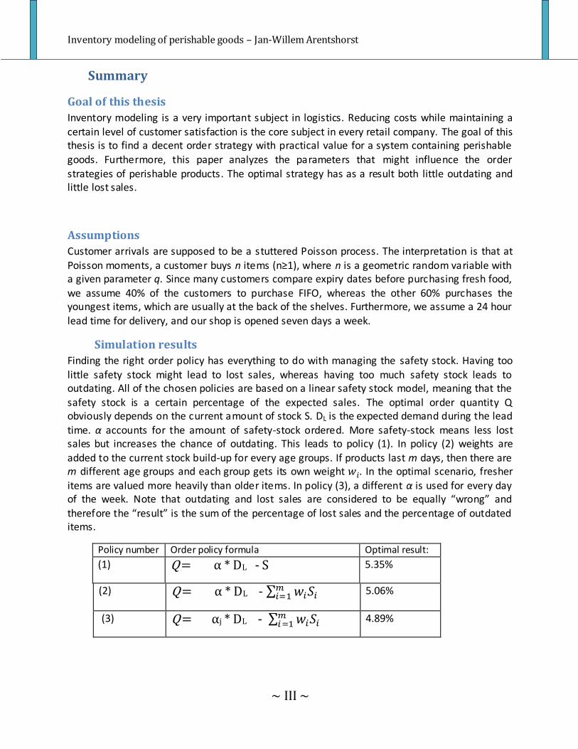
Finding the right order policy has everything to do with managing the safety stock. Having too little safety stock might lead to lost sales, whereas having too much safety stock leads to outdating. All of the chosen policies are based on a linear safety stock model, meaning that the safety stock is a certain percentage of the expected sales. The optimal order quantity Q obviously depends on the current amount of stock S. DL is the expected demand during the lead time. α accounts for the amount of safety-stock ordered. More safety-stock means less lost sales but increases the chance of outdating. This leads to policy (1). In policy (2) weights are added to the current stock build-up for every age groups. If products last m days, then there are m different age groups and each group gets its own weight . In the optimal scenario, fresher
items are valued more heavily than older items. In policy (3), a different α is used for every day of the week. Note that outdating and lost sales are considered to be equally “wrong” and
therefore the “result” is the sum of the percentage of lost sales and the percentage of outdated items.
Policy number Order policy formula Optimal result:
(1) Q = α * DL - S 5.35%
(2) Q = α * DL - 5.06%
(3) Q = αj * DL - 4.89%
Inventory modeling of perishable goods – Jan-Willem Arentshorst
~ IV ~
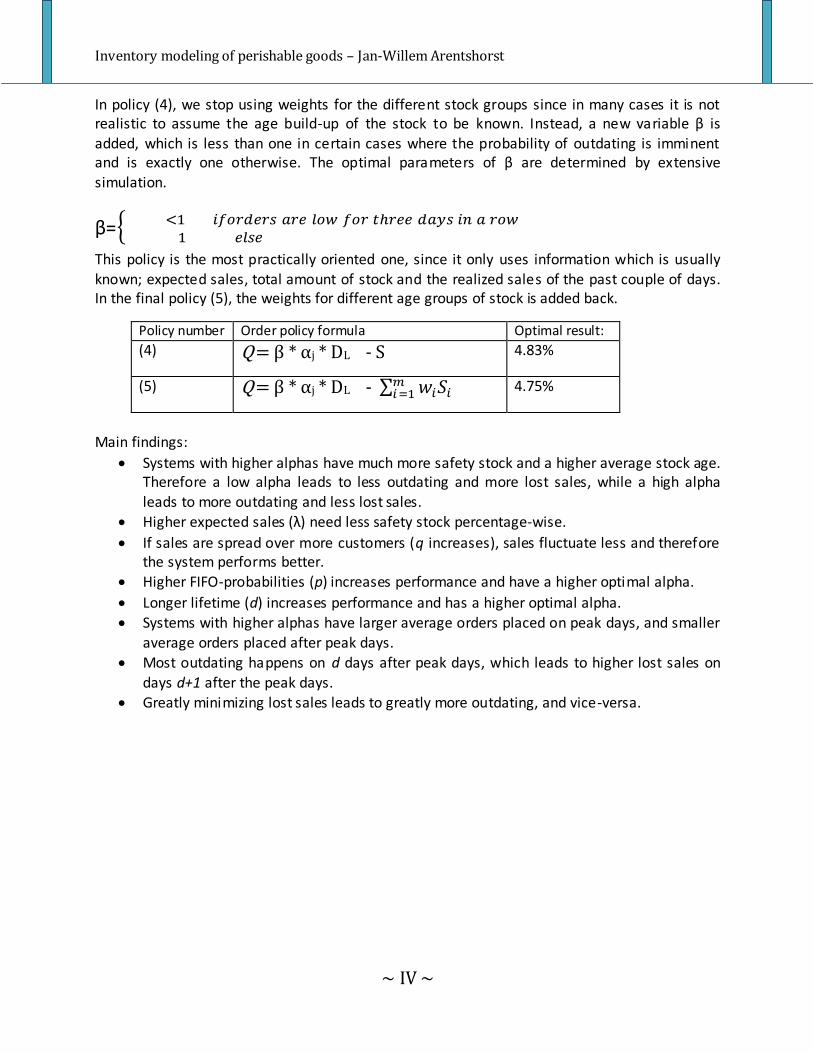
In policy (4), we stop using weights for the different stock groups since in many cases it is not realistic to assume the age build-up of the stock to be known. Instead, a new variable β is added, which is less than one in certain cases where the probability of outdating is imminent and is exactly one otherwise. The optimal parameters of β are determined by extensive simulation.
β=
This policy is the most practically oriented one, since it only uses information which is usually known; expected sales, total amount of stock and the realized sales of the past couple of days. In the final policy (5), the weights for different age groups of stock is added back.
Policy number Order policy formula Optimal result:
(4) Q = β * αj * DL - S 4.83%
(5) Q = β * αj * DL - 4.75%
Main findings:
Systems with higher alphas have much more safety stock and a higher average stock age. Therefore a low alpha leads to less outdating and more lost sales, while a high alpha leads to more outdating and less lost sales.
Higher expected sales (λ) need less safety stock percentage-wise.
If sales are spread over more customers (q increases), sales fluctuate less and therefore the system performs better.
Higher FIFO-probabilities (p) increases performance and have a higher optimal alpha.
Longer lifetime (d) increases performance and has a higher optimal alpha.
Systems with higher alphas have larger average orders placed on peak days, and smaller average orders placed after peak days.
Most outdating happens on d days after peak days, which leads to higher lost sales on
days d+1 after the peak days. Greatly minimizing lost sales leads to greatly more outdating, and vice-versa.
Inventory modeling of perishable goods – Jan-Willem Arentshorst
~ V ~
Comparison to a real life situation:
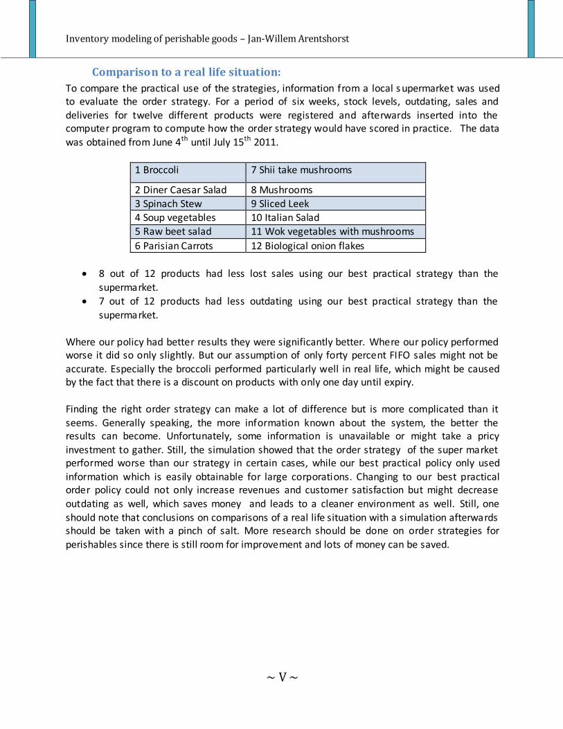
To compare the practical use of the strategies, information from a local s upermarket was used to evaluate the order strategy. For a period of six weeks, stock levels, outdating, sales and
deliveries for twelve different products were registered and afterwards inserted into the computer program to compute how the order strategy would have scored in practice. The data
was obtained from June 4th until July 15th 2011.
1 Broccoli 7 Shii take mushrooms
2 Diner Caesar Salad 8 Mushrooms 3 Spinach Stew 9 Sliced Leek
4 Soup vegetables 10 Italian Salad
5 Raw beet salad 11 Wok vegetables with mushrooms
6 Parisian Carrots 12 Biological onion flakes
8 out of 12 products had less lost sales using our best practical strategy than the
supermarket. 7 out of 12 products had less outdating using our best practical strategy than the
supermarket.
Where our policy had better results they were significantly better. Where our policy performed worse it did so only slightly. But our assumption of only forty percent FIFO sales might not be accurate. Especially the broccoli performed particularly well in real life, which might be caused by the fact that there is a discount on products with only one day until expiry. Finding the right order strategy can make a lot of difference but is more complicated than it seems. Generally speaking, the more information known about the system, the better the results can become. Unfortunately, some information is unavailable or might take a pricy
investment to gather. Still, the simulation showed that the order strategy of the super market performed worse than our strategy in certain cases, while our best practical policy only used
information which is easily obtainable for large corporations. Changing to our best practical order policy could not only increase revenues and customer satisfaction but might decrease
outdating as well, which saves money and leads to a cleaner environment as well. Still, one should note that conclusions on comparisons of a real life situation with a simulation afterwards should be taken with a pinch of salt. More research should be done on order strategies for perishables since there is still room for improvement and lots of money can be saved.
Inventory modeling of perishable goods – Jan-Willem Arentshorst
~ VI ~
Table of contents 1. Introduction ................................................................................................................................ 1
2. The inventory model.................................................................................................................... 2
2.1 The topic of this thesis.......................................................................................................... 2
2.2 Assumption 1: Replenishment .............................................................................................. 2
2.3 Assumption 2: Product lifetime distribution........................................................................... 2
2.4 Assumption 3: FIFO versus LIFO ............................................................................................ 2
2.5 Assumption 4: Demand ........................................................................................................ 3
2.6 Assumption 5: External influences on demand ....................................................................... 4
2.7 Assumption 6: Costs ............................................................................................................. 4
3. Literature review of order policies ................................................................................................ 5
3.1 The history of order policies ................................................................................................. 5
3.2 The Economic Order Quantity ............................................................................................... 5
3.3 The (s,S)-type replenishment policy....................................................................................... 6
3.4 The Newsvendor problem .................................................................................................... 6
3.5 Stochastic multi-period models for perishables ...................................................................... 7
3.6 The topic of this thesis.......................................................................................................... 7
4. Order strategies .......................................................................................................................... 8
4.1 The complexity of perishables............................................................................................... 8
4.2 A non-perishable approach (up-to-S) ..................................................................................... 8
4.3 Age-dependent policies ........................................................................................................ 9
4.4 Policy using previous order information .............................................................................. 10
5. Simulation: settings and programming........................................................................................ 11
5.1 Parameter settings ............................................................................................................. 11
5.2 Batch-means and statistical significance .............................................................................. 12
5.3 Pseudo code ...................................................................................................................... 13
5.4 Performance measures....................................................................................................... 14
6. Simulation: results .................................................................................................................... 15
6.1 Understanding stock behavior using the basic policy ............................................................ 15
6.2 Policies dealing with perishability........................................................................................ 26
6.3 A policy using previous order information ........................................................................... 27
Inventory modeling of perishable goods – Jan-Willem Arentshorst
~ VII ~
7. Comparison to a real life situation .............................................................................................. 29
7.1 Supermarket information ................................................................................................... 29
7.2 Product selection ............................................................................................................... 29
7.3 Data analysis...................................................................................................................... 31
8. Simulation results compared to the real life situation .................................................................. 34
8.1 Settings and assumptions ................................................................................................... 34
8.2 Comparison on lost sales .................................................................................................... 35
8.3 Comparison on outdating ................................................................................................... 37
8.4 Analysis on the constraint that outdating < 2% .................................................................... 39
8.5 Further discussion .............................................................................................................. 40
9. References ................................................................................................................................ 41
Appendix A: Basic Java code .............................................................................................................. 42
Appendix B: Additional graphs and tables........................................................................................... 48
Inventory modeling of perishable goods – Jan-Willem Arentshorst
~ 1 ~
1. Introduction Inventory modeling is one of the most important concepts in logistics. Having a solid inventory
strategy could not only save a company lots of money, but might be the difference between not being able to compete against the competition and having a prominent position in the market
segment.
One of the most important aspects of inventory modeling is the prediction of demand for a certain good. If it would be known beforehand at which moment a certain good will be sold, inventory management would be much simpler. However, planning becomes much more complicated when demand behaves stochastically. Stochasticity causes severe fluctuations in demand with which companies need to deal with. Firms tend to keep their stock high enough to minimize the amount of lost sales, but storage of redundant goods costs both time and money. Since having an adequate balance between these two aspects is essential, it is vital to find the
optimal strategy of how much to replenish and at which moment. The optimal strategy depends on the interests of the management team; what level of lost sales is acceptable and how much
money are the storage cost allowed to accumulate to? Since supply chains are important for nearly every type of industry, the demand for this type of research has increased over the past decades. However, relatively little attention has been devoted to the inventory modeling of perishable goods. Dealing with perishable goods, especially in the food industry, appears to be a significant problem. Outdating in the food industry occurs on a very broad spectrum of products. On one hand there is canned food which is sometimes preservable for over two years, while on the other hand fish and vegetables perish in a few days. Obviously these two different types of products require different approaches and therefore different order strategies. For example, for products which expire rather quickly, the
focus might be less on minimizing lost sales and more on preventing these products passing their expiration dates and minimizing the amount of thrown away goods.
The main purpose of this paper is to identify and quantify the factors influencing the optimal strategy to aid companies in their quest for the optimal replenishment strategy. The best order strategy uses all available information to calculate the optimal replenishment quantities. For instance, the theoretical optimal strategy will probably be influenced by the age distribution of the products, but it is impractical to count the number of items with a certain expiration date for every product on a daily basis. In practice, the optimal model is the one which satisfies best
a certain set of constraints; demand should be met to a certain degree, the amount of perished goods should be small and stock levels should be manageable. Therefore, the goal of this thesis
is to find an operable strategy for perishable goods.
Inventory modeling of perishable goods – Jan-Willem Arentshorst
~ 2 ~
2. The inventory model
2.1 The topic of this thesis
The goal of this thesis is to find a decent order strategy with practical value for a system containing perishable goods. Furthermore, this paper analyzes the parameters that might influence the order strategies of perishable products. But to find such a strategy a correct model
has to be created first. Our model is based on replenishment in supermarkets. This means dealing with perishable goods in an environment with stochastic demand and periodic delivery.
The chosen model is based on a few crucial assumptions, which are listed below.
2.2 Assumption 1: Replenishment
The first assumption regards the replenishment cycle. Deliveries are supposed to arrive at the
start of every day, and orders for the next day need to be placed directly after the delivery. Furthermore, the product can only be ordered in batches of size B. For example, wine is usually
shipped in boxes containing six bottles. Stock shelves are assumed to be abundant and backorders are not allowed.
2.3 Assumption 2: Product lifetime distribution
The second assumption has to do with the lifetime of these goods. In many cases lifetimes are deterministic. This implies that goods perish in exactly d days. This is the case with all kinds of prepacked foods and applies to the regulation regarding donations in blood banks as well; blood has to be used within a certain number of days by law. In completely different cases exponential lifetimes are assumed. Exponential lifetime means an item has a certain probability to perish in a certain amount of time (at a certain rate r), no matter how long the item has been in the system. This applies for instance to radioactive decay, and this assumption makes computations a lot simpler. A lifetime assumption combining both properties is chosen; the so-called shifted exponential distribution. This way products are assumed to last at least d days, and then perish at a certain exponential rate r. Note that assuming r to be infinite or d to be zero leads to
respectively the deterministic or exponential distributions mentioned above.
2.4 Assumption 3: FIFO versus LIFO
Most models assume the oldest goods to be purchased first, which is called First-In-First-Out
(FIFO). In the context of supermarkets FIFO models are usually preferred over other models since they have less outdating than, for example, Last-In-First-Out (LIFO) models. In certain
scenarios, the freshness of the products influences customer satisfaction. In those cases hybrid models are used to combine the advantages of the two policies. FIFO purchases cannot be
guaranteed since customers in supermarkets are usually free to pick a product to their liking, and tend to choose the freshest products available. A fraction p of the customers is assumed to
purchase their groceries FIFO and a fraction (1-p) to purchase LIFO. For quickly perishable goods such as meat and vegetables, up to sixty percent1 of the Dutch consumers explicitly choose
products with the longest shelf life.
1 This percentage was taken from an online article from a research group from the University of Wageningen but is
not available anymore.
Inventory modeling of perishable goods – Jan-Willem Arentshorst
~ 3 ~
2.5 Assumption 4: Demand
There is supposed to be weekly pattern in sales, meaning the expected demands on day i and i+7 are equal. The effects of this weekly pattern was studied by Kahn et al [9]. They found a
clear dependency between customer visits on a specific day and visits exactly one week later, but this specific dependency is not included to reduce unnecessary complexity. The demand for
the observed product is assumed to be a ‘stuttered’ Poisson process. Customer arrivals are alleged to be a time-dependent Poisson process with a known arrival rate (λi) which changes over time. The interpretation is that at Poisson moments, a customer buys n items (n≥1), where
n is a geometric random variable with a given parameter q. The assumption of sales following a Poisson process could be sufficient. But for the Poisson distribution the variance is equal to its
mean, whereas empirical data shows the variance of sales sometimes even doubles the mean. The geometric random variable is used to account for this additional variance, because we now
deal with a random sum of random variables.
Let X1,X2,... be a sequence of independent random variables where each variable has a
geometric distribution with parameter q. It is well know that E =
and Var( ) =
.
Then E = Var( ) + E
2 =
+
=
Let N be a Poisson variable with parameter λ, then E[N] = λ and Var(N) = λ. Now the expected demand is:
E = E * E[N] =
λ =
Now the variance of the demand is: Var
= E[N]Var( ) + E
Var(N)
= λ
+
λ
=
λ
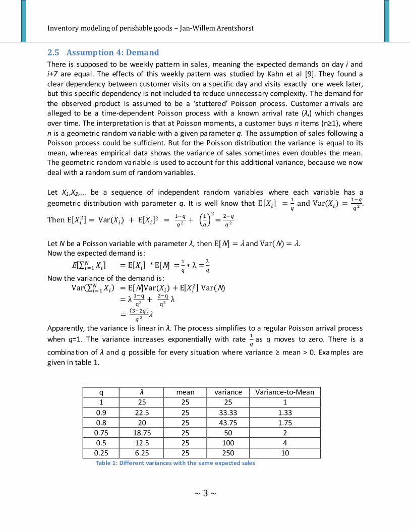
Apparently, the variance is linear in λ. The process simplifies to a regular Poisson arrival process
when q=1. The variance increases exponentially with rate
as q moves to zero. There is a
combination of λ and q possible for every situation where variance ≥ mean > 0. Examples are
given in table 1.
q λ mean variance Variance-to-Mean
1 25 25 25 1
0.9 22.5 25 33.33 1.33
0.8 20 25 43.75 1.75
0.75 18.75 25 50 2
0.5 12.5 25 100 4
0.25 6.25 25 250 10 Table 1: Different variances with the same expected sales

Inventory modeling of perishable goods – Jan-Willem Arentshorst
~ 4 ~
Figure 1 contains the Variance-to-Mean ratio for different values of q. This ratio reflects the
effect of q on the variance. Note that when q decreases, λ has to decrease as well to keep the mean constant. Finally, we assume that Friday and Saturday have twice as customers as the other days of the week.
2.6 Assumption 5: External influences on demand
The product itself is homogenous and is assumed to have no complementary or substitute goods. The effect of substitution is studied by Smith and Agrawal [11]. They conclude that computation is rather complex and requires many substitution probabilities which might be
difficult to obtain, but that substitution effects can have a significant effect on cost reduction and the optimal order policy. Chen and Plambeck [7] show that the usage of substitute goods could lower total stock levels by using hybrid safety stock. The effects of price changes on the optimal inventory policy for perishable goods are studied by Shah [18] and [19]. All of these effects are neglected here for computational reasons.
2.7 Assumption 6: Costs
Another important assumption deals with the costs involved. Most inventory models only include costs for holding inventory to minimize stock, and costs for lost sales to obtain a certain
service level. Our model obviously includes costs for perished goods as well. Costs for delivery
are neglected, since in nearly all cases a single product does not affect the decision of the store to receive a delivery. Also, the costs of placing the product on the shelves will never have a
significant effect on the replenishment policy.
0
1
2
3
4
5
6
7
8
9
10
11
12
13
14
0.2 0.3 0.4 0.5 0.6 0.7 0.8 0.9 1
Var
ian
ce-t
o-m
ean
Geometric parameter q
Variance-to-Mean for different values of q
Figure 1: The curve of the variance-to-mean ratio depending on q
Inventory modeling of perishable goods – Jan-Willem Arentshorst
~ 5 ~
3. Literature review of order policies
3.1 The history of order policies
Inventory modeling is an important topic in Operations Research and has made great progress during the twentieth century. Basically, inventory theory deals with two questions:
How many units should be ordered?
At which time should the order be placed?
This is a brief overview of the development of inventory theory. Listing all models could be a thesis on its own, as shown in [6] and [8], therefore only the more important ones are noted.
Inventory theory started being fully deterministic, and over the years expanded to dealing with stochastic demand and perishability.
3.2 The Economic Order Quantity
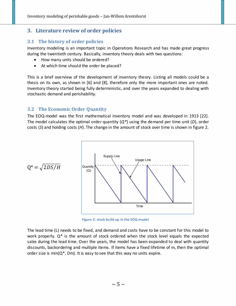
The EOQ-model was the first mathematical inventory model and was developed in 1913 [22].
The model calculates the optimal order quantity (Q*) using the demand per time unit (D), order costs (S) and holding costs (H). The change in the amount of stock over time is shown in figure 2.
Q* =
The lead time (L) needs to be fixed, and demand and costs have to be constant for this model to work properly. Q* is the amount of stock ordered when the stock level equals the expected sales during the lead time. Over the years, the model has been expanded to deal with quantity discounts, backordering and multiple items. If items have a fixed lifetime of m, then the optimal
order size is min(Q*, Dm). It is easy to see that this way no units expire.
Figure 2: stock build-up in the EOQ-model
Inventory modeling of perishable goods – Jan-Willem Arentshorst
~ 6 ~
3.3 The (s,S)-type replenishment policy.
A new inventory policy dealing with stochastic demand over multiple periods was introduced by Arrow, Harris and Marschak in 1951 [21]. This (s,S) policy states that stock should be
replenished to a certain level S at the moment it reaches level s, with s < S. The lead time is considered to be zero and the amount to be replenished is obviously S-s. This type of policies
are called continuous review models. This policy was proven to be optimal for most models with non-perishables and a linear cost structure. Fries [4] proved that the (s,S) policy is not optimal for multi-period models with perishables.
3.4 The Newsvendor problem
The first model regarding perishable goods with stochastic demand was the classical single
period problem [20]. This model is also known as the Newsvendor problem, Newsboy problem or Christmas tree problem. It models a newsvendor who has to decide how many copies of the
papers to stock, knowing that leftover newspapers are worthless and that demand is uncertain. There are two possible types of costs in this situation: the costs of having leftovers (h) and the
costs of having lost sales (k). If the demand distribution D is known, then the optimal order is
.
Here denotes the inverse distribution of the demand. For example, if
= 0.75, then the
optimal order quantity states there should be shortages in 25 percent of the cases. This is an
inventory policy which deals with single-period perishable goods and probabilistic demand. However, the scope of this thesis could be classified as a multi-period newsvendor problem
which appears to be much more complicated. Fries [4] has extended the newsvendor problem to l≥2 days, and assumes zero lead time and a FIFO policy.
Inventory modeling of perishable goods – Jan-Willem Arentshorst
~ 7 ~
3.5 Stochastic multi-period models for perishables
Liu and Lian [17] extended the (s,S) replenishment policy to perishables. They assume immediate replenishment and choose s ≤ -1. This means that a new order will not be made until
at least one customer arrives as soon as the entire stock has been depleted. So they not only allow backorders, but actually encourage it. Schmidt and Nahmias [2] use a special case, fixing s
= S-1. This (S-1,S) model deals with items with fixed shelf life, disallows backordering and places an order as soon as an item has perished or is sold. They use it in context of functioning machines that either brake down or are removed for maintenance. Lian and Neuts [15] adapted
the (s,S) model to a discrete time model by rewriting states to a Markov Chain. Nahmias and Wang [1] on the other hand model a (Q,r) system, which is basically an (s,S) policy with positive
lead times. Ravichandran [3] shows how complex the (s,S) model is for more realistic assumptions, like non-instantaneous lead times, constant shelf life and stochastic demand. He
concludes such models to be quite complex and intractable, and meaningful analysis can only be obtained by simulation. Tekin et al. [14] propose a (Q,r,T) model, in which Q units are ordered
when stock levels drop below r or when T units of time have passed since the last order. This way, the order policy is not only based on the current stock levels but indirectly on the remaining shelf life of the items as well. This is a periodic review model, just like the newsvendor problem, where the other models assume continuous reviewing. This policy is observed to outperform the regular (Q,r) system.
3.6 The topic of this thesis
Apparently, a multi-period, perishable inventory model without backorders and non-stationary probabilistic demand seems to be intractable and too complex to solve analytically. Therefore resorting to simulation is required to find a suboptimal heuristic.
Inventory modeling of perishable goods – Jan-Willem Arentshorst
~ 8 ~
4. Order strategies
4.1 The complexity of perishables
The truly optimal inventory strategy takes every possible piece of information into account, including the weather forecast, upcoming social events, the age distribution of the customers and inflation. But due to computational limitations and a lack of data, a trade-off between
completeness and simplicity has to be made. This trade-off is acceptable because the vast majority of the variation lies within the nature of the demand process itself. For example, an
adequate strategy for non-perishable goods basically needs just three pieces of information; the current amount of stock, information about the lead time and the distribution of the demand for the following period. The ratio between lost sales and overstocking depends on their respective costs.
For perishables, the policy becomes more complex. Because costs for outdating are usually
much higher than holding costs, limiting outdating becomes crucial, especially in a non-FIFO environment. Intuitively, products with longer expected shelf lives should be allowed to have more safety stock than their quickly deteriorating counterparts. In non-FIFO environments, when the current stock approaches its expiration date, less safety stock should be held to decrease outdating. So the perishable order strategy not only depends on the current stock and
expected demand, but on the expected shelf life, the expected fraction of FIFO sales and the age distribution of the stock as well. In the following subsections different order strategies are
discussed that try to deal with this complexity.
4.2 A non-perishable approach (up-to-S)
The first policy is a control group model. It does not take into account any of the perishable-specific information and only depends on current stock level and the expected sales during the lead time. If D is the expected demand per time unit and the single lead time is T, then DL equals
2*D*T in most cases. Note that with this lead time the time between the placement of this order and the arrival of the next order is meant. So it is not just the time until this order is
delivered, but the time until the next order could arrive. The system is replenished with a certain order quantity Q given by:
Q = α * DL - S , (1)
where DL is the expected demand during lead time, S the current stock level and α ≥ 0.
If α = 1, then no safety stock is held. To effectively deal with the stochasticity, α might range from 1.0 to 2.5 depending on the expected sales, and the cost of outdating and lost sales. Take
α = 1.5 for example. Note that if we are dealing with regular Poisson sales with λ = 4, P(X ≥ 6) ≈ 0.21, whereas if λ = 40, P(X ≥ 60) ≈ 0.002. This shows that for higher expected demands, a
smaller fraction of safety stock is needed and a lower α can be taken. It is trivial that α < 1 is not optimal in any practical scenario. Instead of using safety stock with a linear dependency on the
expected demand, a safety stock function with a root or a logarithmic function could also be used, but that is beyond the scope of this thesis.
Inventory modeling of perishable goods – Jan-Willem Arentshorst
~ 9 ~
4.3 Age-dependent policies
The age-dependent policy also takes into account the information regarding possible outdating. There is very little literature regarding such policies in a practical setting, i.e. non-instantaneous
lead times and not fully FIFO sales. When sales are assumed to be fully FIFO, the amount of safety stock is only a little less than its non-perishable equivalent. The difference in safety stock
depends on the expected lifetime of the items. As the expected lifetime of goods increases, the stock level starts to behave more similar to non-perishables.
The policy for LIFO sales is more sensitive to outdating since the freshest products are sold first.
Finding the right balance between minimizing lost sales and minimizing outdating is more difficult. Much less safety stock is held, since the risk of outdating is more imminent. Define as the amount of stock with i remaining days of shelf life. This creates a total of m age categories.
Now remember the non-perishable order formula:
Q = α * DL - S (1)
where DL is the expected demand during lead time, α ≥ 0 and S = ; the current stock
level. We can make (1) age-dependent by changing S into a weighted function:
Q = α * DL - (2)
Adding more or less weight to certain classes of stock might cause the system to order more
when the stock is relatively young, and order less when the stock is relatively old. Also, if the system expects a significant amount of items to be outdated at the end of the day, it might want to increase the order for the following morning. These weights can be more influential in LIFO
situations than in FIFO situations. This is because having an old stock is much more troublesome in LIFO situations, since getting rid of the old stock before outdating gives a high exposure to
lost sales. Note that in (1) all are equal to 1.
If goods have a shelf life of five days, one could understand that orders which arrive on Thursday can safely be somewhat increased, since the Friday and Saturday are coming up and
any leftovers from Thursday should be easily sold during the weekend. On the other hand, placing a massive order on Sunday might be risky. This is why we introduce α j to the order formula, with j being the day of the week. The utility of this variable heavily depends on the expected lifetime of the goods. This variable is for example more useful in LIFO than in FIFO systems. All of these additions lead to the following formula:
Q = αj * DL - (3)

Inventory modeling of perishable goods – Jan-Willem Arentshorst
~ 10 ~
4.4 Policy using previous order information
Using weights for different ages of stock mentioned earlier is not very practical. It would require optical inspection of all inventory on a daily basis to know exactly how much of each type is in
stock, which is not practical at all. This means we will need to find another way to add information about the age distribution of our stock.
As stated before, Tekin et al. [14] proposed a (Q,r,T) policy. This policy orders Q units when stock levels drop below r or when T units of time have passed since the last order. The last part
makes sure the order policy is not only based on the current stock levels but on the remaining shelf life of the items as well. The model was proven to outperform models lacking that addition
in the area of reaching a certain service level. So information is needed that could be an indicator for having rather young or old stock. We could add something similar here as well. We
can use any information about daily sales and order quantities, since these are usually digitally available and often easy to obtain.
For example, it could be an indication of old stock, if order quantities have been rather low for a few days. Having placed a gigantic new order could indicate rather young stock. So the weighting of stock is removed and a new variable β is introduced, which value decreases an order if orders have been low enough for a certain amount of time. The optimal parameters of β can be determined by extensive simulation.
Q = β * αj * DL - S (4)

Inventory modeling of perishable goods – Jan-Willem Arentshorst
~ 11 ~
5. Simulation: settings and programming The policies from chapter 5 were tested in the model specified in chapter 3 by means of simulation. A program was written in JAVA which simulated the stock levels for a series of n days, using the expected demand for each day. Most parameters were varied to give a sensitivity analysis of the order strategies.
5.1 Parameter settings
λi ≥ 0 The expected number of customer arrivals for day i. Statistics from two local supermarkets showed that total sales on Monday, Tuesday, Wednesday, Thursday and Sunday are roughly the same (λ). Sales on Friday and Saturday are roughly twice as much as on the other days (2λ). Note that this weekly pattern was used for convenience only, but other values can be given as input as well.
q ∈ (0,1] The variance in total sales
In some cases the variance is nearly twice as much as the average sales. According to Figure 1, q has to be around 0.75 in these cases.
p ∈ [0,1] The fraction of customers buying FIFO
The (expected) fraction of FIFO sales has a major influence on the probability of outdating. Scenarios with FIFO (p=1), LIFO (p=0) and hybrid sales (p=0.4) were simulated.
d ≥ 0 The minimum (deterministic) lifetime of the goods
The standard minimum lifetime was chosen to be d = 5 days.
r ≥ 0 ∈ [0,1] The exponential decay rate For convenience, we choose r as the expected percentage of the population to perish after d days. We neglect this exponential decay in the standard situation, but this will be part of the sensitivity analysis.
B ≥ 1 The number of items per batch Most simulations were run with B=1, since other values for this parameter did not seem to have a significant effect on the optimal settings, but only seemed to blur the results.
For completeness, a sensitivity analysis was done with B=4.
Default settings: During simulation we chose “default settings” to make comparing easier:
λ = 5, q = 0.75, p = 0.4, d = 5, r = 100%, B = 1
Inventory modeling of perishable goods – Jan-Willem Arentshorst
~ 12 ~
Furthermore, we assumed the lead time to be exactly one day, which is quite realistic for supermarkets. It is convenient to assume delivery arrives “between days”; either after closing or just before opening. By organizing the replenishment and outdating outside of the sale window, there is no need to make a distinction between the daily sales before and after delivery. This assumption makes calculations simpler, and the application of the theory more practical. Moreover, it is not unusual for supermarkets to receive their deliveries either late in the evening or early in the morning. In many of these cases, the expected sales after or before delivery can
be neglected and therefore fit our assumptions.
5.2 Batch-means and statistical significance
One long simulation run of n days is simulated to obtain the number of outdated items D1,....Dn
for a large n. An obvious estimator for the expected percentage of thrown-away items would be the sum of these values divided by the total number of items held in stock.
=
Unfortunately the corresponding confidence interval is not as accurate as it should be, because these values are strongly correlated. The batch-means method is used to solve this problem. In the batch-means method, the simulation is divided into k smaller subruns. Each subrun covers a
period of b =
days. The averages of each subrun are nearly uncorrelated as long as b is large
enough. These subrun averages are used to create reliable confidence intervals. Another
advantage is that because the subruns are uncorrelated, only one period of warm-up data has to be thrown away. For this simulation, b = 25000 days and k = 41. b is chosen such that the
confidence interval around the average is negligible. The warm-up period is arbitrarily chosen to be nearly a year; that is 52 weeks.

Inventory modeling of perishable goods – Jan-Willem Arentshorst
~ 13 ~
5.3 Pseudo code
Pseudo code of the three main methods is shown below; the full code is available in the appendix. Basically, each day consists of four functions: replenishing, ordering, outdating and
selling. The order of the first three functions is interchangeable. This particular order is chosen because it is intuitive. Replenishing and ordering might as well be the final tasks of the day
instead of the first. program start():
do_warmup_period (); for (1 to r subruns)
for (1 to b days) simulateDay();
} }
end program method simulateDay(): replenish_stock(); place_order(); double lambda = expectedArrivals(current_day);
int customers = simulatePoisson(lambda) for (1 to customers){ processCustomer();
} age_stock_and_outdate();
end method method processCustomer(): int sales = geometricDrawing(q); lostsales = max (sales – stock, 0) sales = min (sales, stock) stock –= sales; double random = new Random(0,1); if (random < FIFO-fraction) -> takeOldest(sales); else -> takeNewest(sales);
end method
Inventory modeling of perishable goods – Jan-Willem Arentshorst
~ 14 ~
5.4 Performance measures
The inventory strategy only has to deal with three measures; the amount of lost sales, the amount of outdating and holding costs. Holding costs seem less important in the context of
supermarkets, since the risk of outdating usually has much more influence on the orders than holding costs. Outdating costs can be difficult to calculate. For example, what are the material
values and what is the price of eliminating the items? The costs of lost sales are even more difficult to determine. In certain cases, customers tend to buy a similar good instead if the good is out of stock. So what is the cost of lost sale then? And what if the substitute good is more
expensive? And what is the value of having a high customer satisfaction level? Anyway, finding the right balance between these two measures is a vital as it is arbitrary. Some managers focus
on customer service; everything has to be perfect for the customer and not a single product should be out of stock. For these managers, outdating is just a necessary evil. Other managers
prefer to minimize outdating, for both economical and ecological reasons. They accept lost sales more easily, since customers tend to buy substitution goods instead. So finding the right
balance depends on how heavily each measure is supposed to be weighted. In this thesis, both measures are weighted equally. After all, both lost sales and outdating can be seen as a wrong order in some sense. In the results section, percentages of outdating and lost sales are listed. Both of these values are compared to the total amount ordered instead of the total demand, since the emphasis in this thesis lies in finding the correct order amount and not on optimizing sales. This implies that if one hundred products are in stock, and there has
been a total demand of 105 items, then the total lost sales are considered
5% (of the
ordered amount) whereas usually this percentage would be
4.8%. So in our cases, lost
sales are not the percentage of demand which could not be fulfilled, but the percentage that
the ordered amount should have been bigger. After all, we need to optimize our orders and not our sales. Note that for long-term simulation, this gives nearly the same result.

Inventory modeling of perishable goods – Jan-Willem Arentshorst
~ 15 ~
6. Simulation: results
6.1 Understanding stock behavior using the basic policy
The first inventory strategy simulated was the non-perishable approach explained in Section 5.2. The effect of this strategy depends on finding the optimal alpha, which is a measure for the safety stock:
Q = α * DL - S , (1)
where DL is the expected demand during lead time, S is the current stock level and α ≥ 1.
All the other policies are based on this type of policy strategy. Alpha is also the most influential
variable in our policies. Before expanding the complexity of our order policies, we first need to understand which model parameters influence alpha the most and what the effects of alpha on
the optimal results are.
The optimal value of alpha depends on the perishability (d and r), expected s ales (λ and q) and the fraction of customers buying FIFO (p). Main findings:
A low alpha leads to less outdating and more lost sales, while a high alpha leads to more
outdating and less lost sales. The optimal value of alpha depends on the balance between lost sales and outdating
caused by the characteristics of the system.
Systems with higher alphas have much more safety stock and a higher average stock age.
Larger batch sizes (B) slightly decreases performance, but has no effect on the optimal alpha.
Higher expected sales (λ) cause relatively less fluctuations in demand, which leads to less
outdating. These systems perform better and can afford lower alphas. If sales are spread over more customers (q increases), sales fluctuate less and therefore
the system performs better. Higher FIFO-probabilities (p) increases performance and have a higher optimal alpha.
Longer lifetime (d) increases performance and has a higher optimal alpha.
Exponential decay (r<100%) instead of deterministic decay with the same average shelf life (r=100%) performs worse and has a lower optimal alpha.
Systems with higher alphas have larger average orders placed on peak days, and smaller average orders placed after peak days.
Most outdating happens on d days after peak days, which leads to higher lost sales on days d+1 after the peak days.
Severely minimizing lost sales leads to much more outdating, and vice-versa.
Inventory modeling of perishable goods – Jan-Willem Arentshorst
~ 16 ~
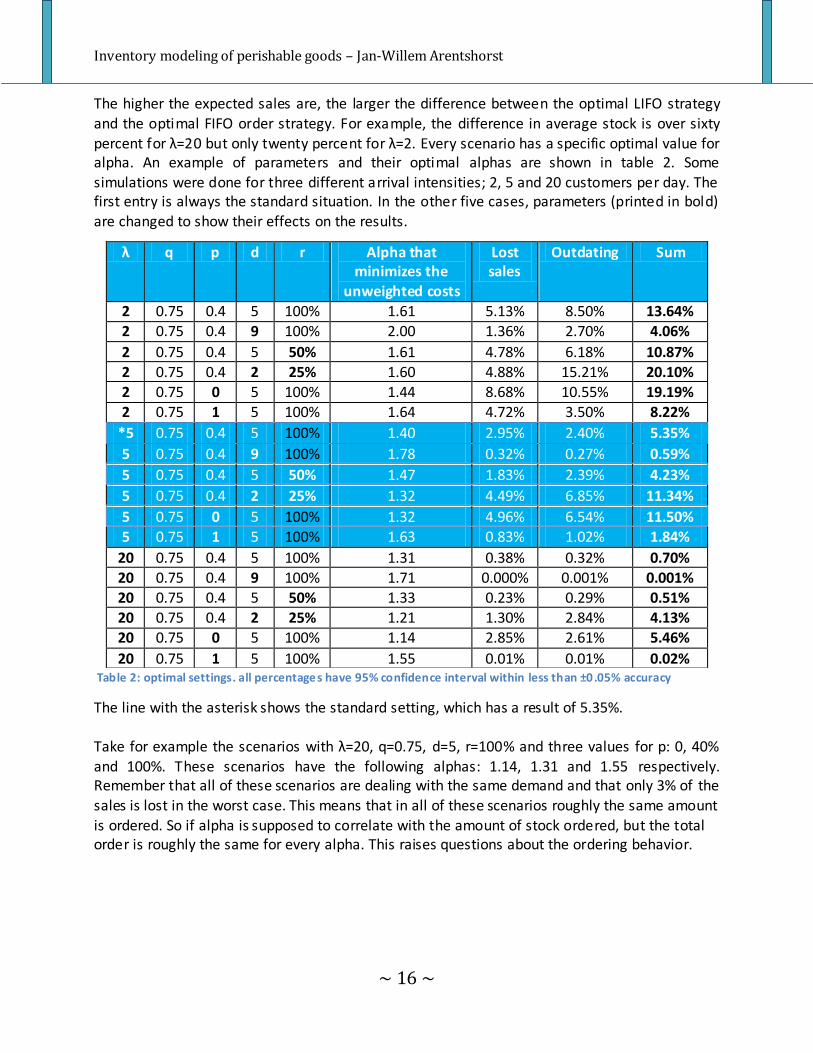
The higher the expected sales are, the larger the difference between the optimal LIFO strategy
and the optimal FIFO order strategy. For example, the difference in average stock is over sixty percent for λ=20 but only twenty percent for λ=2. Every scenario has a specific optimal value for alpha. An example of parameters and their optimal alphas are shown in table 2. Some simulations were done for three different arrival intensities; 2, 5 and 20 customers per day. The first entry is always the standard situation. In the other five cases, parameters (printed in bold) are changed to show their effects on the results.
Table 2: optimal settings. all percentages have 95% confidence interval within less than ±0.05% accuracy
The line with the asterisk shows the standard setting, which has a result of 5.35%.
Take for example the scenarios with λ=20, q=0.75, d=5, r=100% and three values for p: 0, 40%
and 100%. These scenarios have the following alphas: 1.14, 1.31 and 1.55 respectively. Remember that all of these scenarios are dealing with the same demand and that only 3% of the
sales is lost in the worst case. This means that in all of these scenarios roughly the same amount
is ordered. So if alpha is supposed to correlate with the amount of stock ordered, but the total order is roughly the same for every alpha. This raises questions about the ordering behavior.
λ q p d r Alpha that minimizes the
unweighted costs
Lost sales
Outdating Sum
2 0.75 0.4 5 100% 1.61 5.13% 8.50% 13.64%
2 0.75 0.4 9 100% 2.00 1.36% 2.70% 4.06%
2 0.75 0.4 5 50% 1.61 4.78% 6.18% 10.87%
2 0.75 0.4 2 25% 1.60 4.88% 15.21% 20.10% 2 0.75 0 5 100% 1.44 8.68% 10.55% 19.19%
2 0.75 1 5 100% 1.64 4.72% 3.50% 8.22%
*5 0.75 0.4 5 100% 1.40 2.95% 2.40% 5.35%
5 0.75 0.4 9 100% 1.78 0.32% 0.27% 0.59%
5 0.75 0.4 5 50% 1.47 1.83% 2.39% 4.23%
5 0.75 0.4 2 25% 1.32 4.49% 6.85% 11.34%
5 0.75 0 5 100% 1.32 4.96% 6.54% 11.50% 5 0.75 1 5 100% 1.63 0.83% 1.02% 1.84%
20 0.75 0.4 5 100% 1.31 0.38% 0.32% 0.70%
20 0.75 0.4 9 100% 1.71 0.000% 0.001% 0.001% 20 0.75 0.4 5 50% 1.33 0.23% 0.29% 0.51%
20 0.75 0.4 2 25% 1.21 1.30% 2.84% 4.13% 20 0.75 0 5 100% 1.14 2.85% 2.61% 5.46%
20 0.75 1 5 100% 1.55 0.01% 0.01% 0.02%
Inventory modeling of perishable goods – Jan-Willem Arentshorst
~ 17 ~
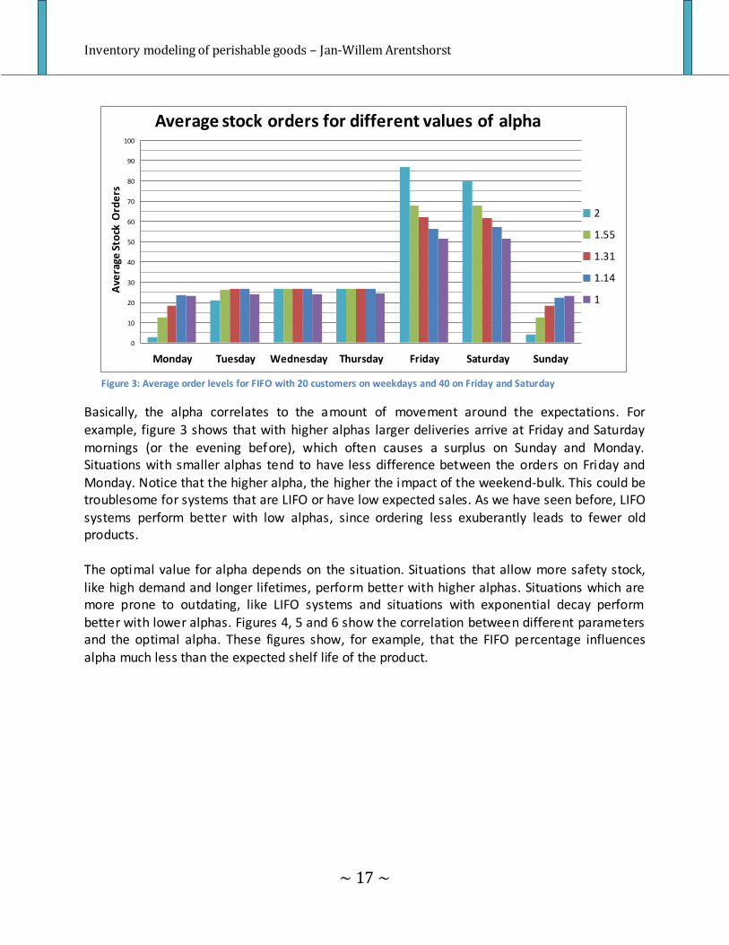
Basically, the alpha correlates to the amount of movement around the expectations. For
example, figure 3 shows that with higher alphas larger deliveries arrive at Friday and Saturday mornings (or the evening before), which often causes a surplus on Sunday and Monday. Situations with smaller alphas tend to have less difference between the orders on Friday and Monday. Notice that the higher alpha, the higher the impact of the weekend-bulk. This could be troublesome for systems that are LIFO or have low expected sales. As we have seen before, LIFO
systems perform better with low alphas, since ordering less exuberantly leads to fewer old products.
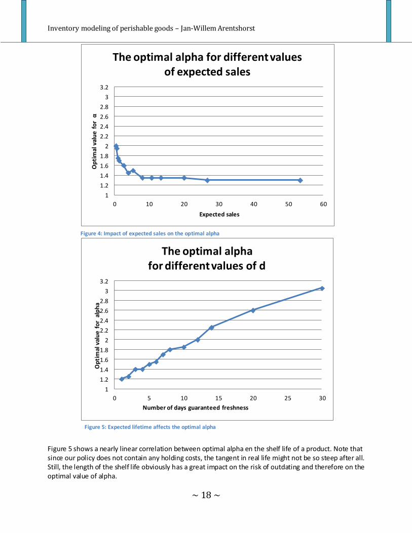
The optimal value for alpha depends on the situation. Situations that allow more safety stock,
like high demand and longer lifetimes, perform better with higher alphas. Situations which are more prone to outdating, like LIFO systems and situations with exponential decay perform
better with lower alphas. Figures 4, 5 and 6 show the correlation between different parameters and the optimal alpha. These figures show, for example, that the FIFO percentage influences
alpha much less than the expected shelf life of the product.
0
10
20
30
40
50
60
70
80
90
100
Monday Tuesday Wednesday Thursday Friday Saturday Sunday
Ave
rage
Sto
ck O
rde
rs
Average stock orders for different values of alpha
2
1.55
1.31
1.14
1
Figure 3: Average order levels for FIFO with 20 customers on weekdays and 40 on Friday and Saturday
Inventory modeling of perishable goods – Jan-Willem Arentshorst
~ 18 ~
Figure 5 shows a nearly linear correlation between optimal alpha en the shelf life of a product. Note that since our policy does not contain any holding costs, the tangent in real life might not be so steep after all. Still, the length of the shelf life obviously has a great impact on the risk of outdating and therefore on the optimal value of alpha.
1
1.2
1.4
1.6
1.8
2
2.2
2.4
2.6
2.8
3
3.2
0 5 10 15 20 25 30
Op
tim
al v
alu
e f
or
alp
ha
Number of days guaranteed freshness
The optimal alpha for different values of d
1
1.2
1.4
1.6
1.8
2
2.2
2.4
2.6
2.8
3
3.2
0 10 20 30 40 50 60
Op
tim
al v
alu
e f
or
α
Expected sales
The optimal alpha for different values of expected sales
Figure 5: Expected lifetime affects the optimal alpha
Figure 4: Impact of expected sales on the optimal alpha
Inventory modeling of perishable goods – Jan-Willem Arentshorst
~ 19 ~
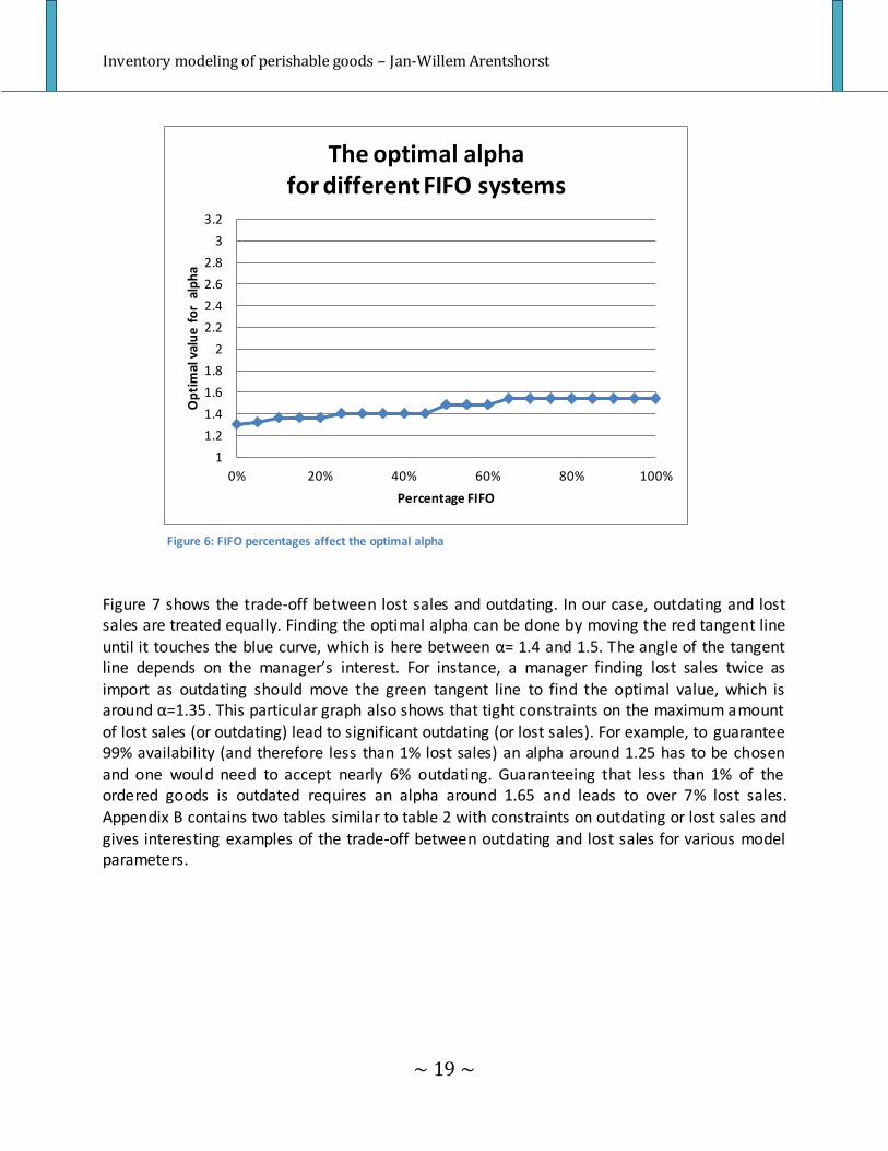
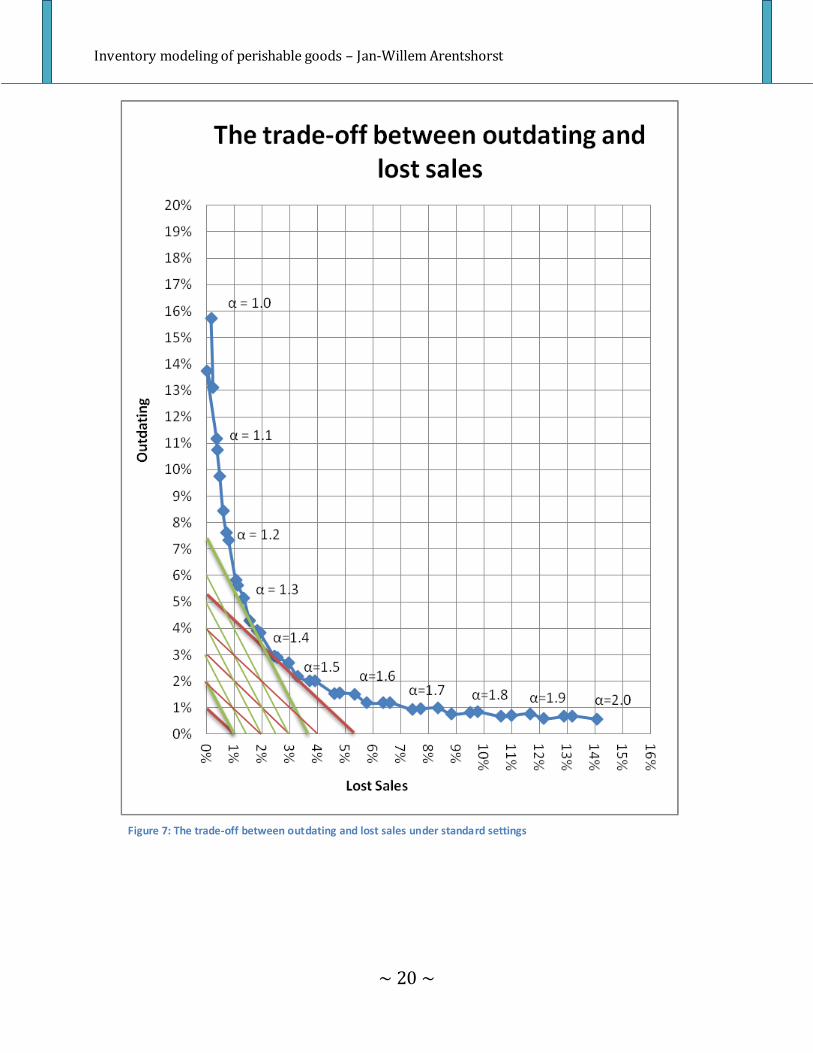
Figure 7 shows the trade-off between lost sales and outdating. In our case, outdating and lost sales are treated equally. Finding the optimal alpha can be done by moving the red tangent line
until it touches the blue curve, which is here between α= 1.4 and 1.5. The angle of the tangent line depends on the manager’s interest. For instance, a manager finding lost sales twice as
import as outdating should move the green tangent line to find the optimal value, which is around α=1.35. This particular graph also shows that tight constraints on the maximum amount of lost sales (or outdating) lead to significant outdating (or lost sales). For example, to guarantee 99% availability (and therefore less than 1% lost sales) an alpha around 1.25 has to be chosen and one would need to accept nearly 6% outdating. Guaranteeing that less than 1% of the ordered goods is outdated requires an alpha around 1.65 and leads to over 7% lost sales. Appendix B contains two tables similar to table 2 with constraints on outdating or lost sales and
gives interesting examples of the trade-off between outdating and lost sales for various model parameters.
1
1.2
1.4
1.6
1.8
2
2.2
2.4
2.6
2.8
3
3.2
0% 20% 40% 60% 80% 100%
Op
tim
al v
alu
e f
or
alp
ha
Percentage FIFO
The optimal alpha for different FIFO systems
Figure 6: FIFO percentages affect the optimal alpha
Inventory modeling of perishable goods – Jan-Willem Arentshorst
~ 20 ~
Figure 7: The trade-off between outdating and lost sales under standard settings
Inventory modeling of perishable goods – Jan-Willem Arentshorst
~ 21 ~
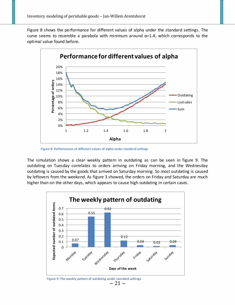
Figure 8 shows the performance for different values of alpha under the standard settings. The
curve seems to resemble a parabola with minimum around α=1.4, which corresponds to the optimal value found before.
The simulation shows a clear weekly pattern in outdating as can be seen in figure 9. The outdating on Tuesday correlates to orders arriving on Friday morning, and the Wednesday
outdating is caused by the goods that arrived on Saturday morning. So most outdating is caused by leftovers from the weekend. As figure 3 showed, the orders on Friday and Saturday are much
higher than on the other days, which appears to cause high outdating in certain cases.
0.07
0.55 0.62
0.12 0.04 0.02 0.04
0
0.1
0.2
0.3
0.4
0.5
0.6
0.7
Exp
ect
ed
nu
mb
er
of
ou
tdat
ed
ite
ms
Days of the week
The weekly pattern of outdating
Figure 9: The weekly pattern of outdating under standard settings
0%
2%
4%
6%
8%
10%
12%
14%
16%
18%
20%
1 1.2 1.4 1.6 1.8 2
Pe
rce
nta
ge o
f o
rde
rs
Alpha
Performance for different values of alpha
Outdating
Lost sales
Sum
Figure 8: Performances of different values of alpha under standard settings
Inventory modeling of perishable goods – Jan-Willem Arentshorst
~ 22 ~
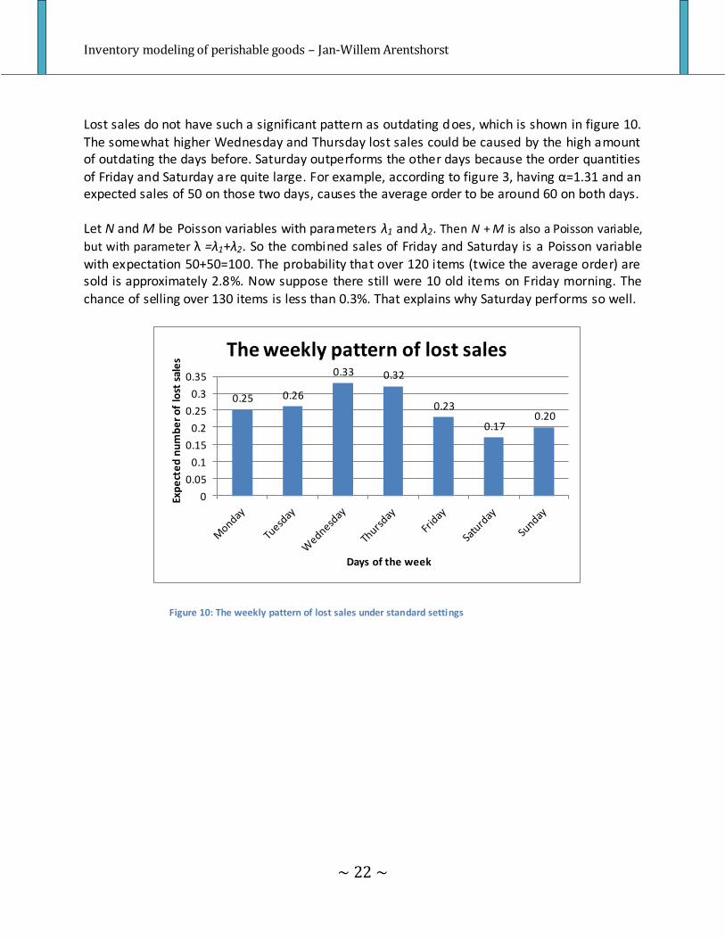
Lost sales do not have such a significant pattern as outdating does, which is shown in figure 10.
The somewhat higher Wednesday and Thursday lost sales could be caused by the high amount of outdating the days before. Saturday outperforms the other days because the order quantities
of Friday and Saturday are quite large. For example, according to figure 3, having α=1.31 and an expected sales of 50 on those two days, causes the average order to be around 60 on both days.
Let N and M be Poisson variables with parameters λ1 and λ2. Then N + M is also a Poisson variable,
but with parameter λ =λ1+λ2. So the combined sales of Friday and Saturday is a Poisson variable
with expectation 50+50=100. The probability that over 120 items (twice the average order) are sold is approximately 2.8%. Now suppose there still were 10 old items on Friday morning. The
chance of selling over 130 items is less than 0.3%. That explains why Saturday performs so well.
Figure 10: The weekly pattern of lost sales under standard settings
0.25 0.26
0.33 0.32
0.23
0.17 0.20
0
0.05
0.1
0.15
0.2
0.25
0.3
0.35
Exp
ect
ed
nu
mb
er
of
lost
sal
es
Days of the week
The weekly pattern of lost sales

Inventory modeling of perishable goods – Jan-Willem Arentshorst
~ 23 ~
Figure 11 shows the average stock buildup for different values of alpha under standard settings.
The difference between start and end of the day increases slightly as alpha rises because a
higher alpha correlates with less lost sales.
Figure 12 shows the average stock age. Items are tagged as being 0, 1, 2, 3 or 4 days in stock and the average of these value is measured. The values are measured in the morning right after
delivery and before opening. The end-day values are measured right before the products age and expire. The average age at the end of the day is slightly older than the one at the beginning
because only 40% is FIFO, so most sales are LIFO.
0
5
10
15
20
25
30
1.0 1.2 1.4 1.6 1.8 2.0
Ave
rage
sto
ck l
eve
l
Alpha
Stock buildup for different alpha
Start of the day
End of the day
0.00
0.20
0.40
0.60
0.80
1.00
1.20
1.40
1.0 1.2 1.4 1.6 1.8 2.0
Ave
rage
sto
ck a
ge
Alpha
Average age of stock for different alpha
Start of the day
End of the day
Figure 11: Average number of items in stock for different values of α under standard settings
Figure 12: Average age of stock for different values of α under standard settings
Inventory modeling of perishable goods – Jan-Willem Arentshorst
~ 24 ~
4.2
2.8 1.7
1.2 0.9
12.5
6.2
2.2 0.6 0.1
27.7
8.5
1.6
0.1 0.0
0.0
5.0
10.0
15.0
20.0
25.0
30.0
Num
ber
of p
rodu
cts
Number of days in the system
Average stock build-up at the end of the day for different systems with 20 expected customers
LIFO
40% FIFO
FIFO
34.2
4.2 2.8
1.7 1.2
34.3
12.5
6.2
2.2
0.6
34.3
27.7
8.5
1.6 0.1
0.0
5.0
10.0
15.0
20.0
25.0
30.0
35.0
40.0
Nu
mb
er
of
pro
du
cts
Number of days in the system
Average stock build-up at the start of the day for different systems with 20 expected customers
LIFO
40% FIFO
FIFO
38.54%
25.95%
15.90% 11.26%
8.34%
47.3%
28.2%
14.7%
7.0%
2.8%
59.32%
26.83%
9.94%
3.15% 0.75%
0.00%
10.00%
20.00%
30.00%
40.00%
50.00%
60.00%
70.00%
Perc
enta
ge o
f p
rodu
cts
Number of days in the system
Average stock build-up at the end of the day for different systems with 20 expected customers
LIFO
40% FIFO
FIFO
Figure 15: Stock build-up at the end of the day
Figure 13: Stock build-up at the start of the day Figure 14: Stock build-up at the start of the day
77.57%
9.43% 6.35%
3.89% 2.76%
61.5%
22.4%
11.1%
4.0% 1.1%
47.44%
38.35%
11.80%
2.23% 0.17%
0.00%
10.00%
20.00%
30.00%
40.00%
50.00%
60.00%
70.00%
80.00%
90.00%
Perc
enta
ge o
f pr
oduc
ts
Number of days in the system
Average stock build-up at the start of the day, for different systems with 20 expected customers
LIFO
40% FIFO
FIFO
Figure 16: Stock build-up at the end of the day
Inventory modeling of perishable goods – Jan-Willem Arentshorst
~ 25 ~
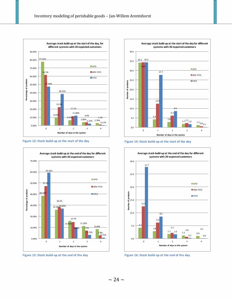
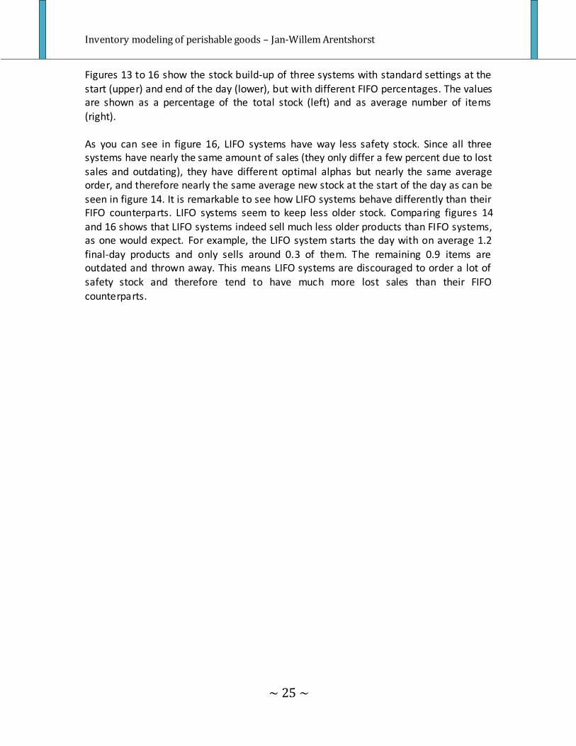
Figures 13 to 16 show the stock build-up of three systems with standard settings at the
start (upper) and end of the day (lower), but with different FIFO percentages. The values are shown as a percentage of the total stock (left) and as average number of items
(right).
As you can see in figure 16, LIFO systems have way less safety stock. Since all three systems have nearly the same amount of sales (they only differ a few percent due to lost
sales and outdating), they have different optimal alphas but nearly the same average order, and therefore nearly the same average new stock at the start of the day as can be seen in figure 14. It is remarkable to see how LIFO systems behave differently than their FIFO counterparts. LIFO systems seem to keep less older stock. Comparing figures 14 and 16 shows that LIFO systems indeed sell much less older products than FIFO systems, as one would expect. For example, the LIFO system starts the day with on average 1.2 final-day products and only sells around 0.3 of them. The remaining 0.9 items are outdated and thrown away. This means LIFO systems are discouraged to order a lot of safety stock and therefore tend to have much more lost sales than their FIFO
counterparts.
Figure 10
Inventory modeling of perishable goods – Jan-Willem Arentshorst
~ 26 ~
6.2 Policies dealing with perishability
The second policy implemented was a policy with different weights for different stock ages. The formula from section 4.3 was used, that is
Q = α * DL - . (2)
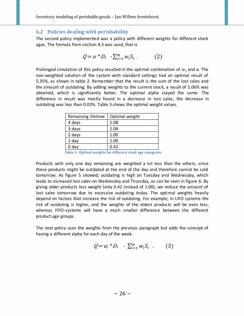
Prolonged simulation of this policy resulted in the optimal combination of and α. The non-weighted solution of the system with standard settings had an optimal result of 5.35%, as shown in table 2. Remember that the result is the sum of the lost sales and the amount of outdating. By adding weights to the current stock, a result of 5.06% was obtained, which is significantly better. The optimal alpha stayed the same. The difference in result was mostly found in a decrease in lost sales; the decrease in outdating was less than 0.03%. Table 3 shows the optimal weight values.
Remaining lifetime Optimal weight
4 days 1.08
3 days 1.04
2 days 1.00 1 day 1.00
0 day 0.42 Table 3: Optimal weights for different stock age categories
Products with only one day remaining are weighted a lot less than the others, since these products might be outdated at the end of the day and therefore cannot be sold tomorrow. As figure 5 showed, outdating is high on Tuesday and Wednesday, which leads to increased lost sales on Wednesday and Thursday, as can be seen in figure 6. By giving older products less weight (only 0.42 instead of 1.00), we reduce the amount of lost sales tomorrow due to excessive outdating today. The optimal weights heavily depend on factors that increase the risk of outdating. For example, in LIFO systems the risk of outdating is higher, and the weights of the oldest products will be even less, whereas FIFO-systems will have a much smaller difference between the different
product age groups.
The next policy uses the weights from the previous paragraph but adds the concept of having a different alpha for each day of the week.
Q = αj * DL - . (3)
Inventory modeling of perishable goods – Jan-Willem Arentshorst
~ 27 ~
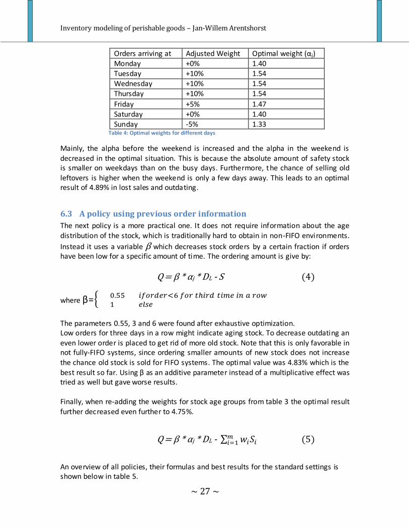
Orders arriving at Adjusted Weight Optimal weight (αj)
Monday +0% 1.40 Tuesday +10% 1.54
Wednesday +10% 1.54 Thursday +10% 1.54
Friday +5% 1.47
Saturday +0% 1.40 Sunday -5% 1.33
Table 4: Optimal weights for different days
Mainly, the alpha before the weekend is increased and the alpha in the weekend is decreased in the optimal situation. This is because the absolute amount of safety stock is smaller on weekdays than on the busy days. Furthermore, the chance of selling old leftovers is higher when the weekend is only a few days away. This leads to an optimal result of 4.89% in lost sales and outdating.
6.3 A policy using previous order information
The next policy is a more practical one. It does not require information about the age distribution of the stock, which is traditionally hard to obtain in non-FIFO environments.
Instead it uses a variable β which decreases stock orders by a certain fraction if orders have been low for a specific amount of time. The ordering amount is give by:
Q = β * αj * DL - S (4)
where β=
The parameters 0.55, 3 and 6 were found after exhaustive optimization. Low orders for three days in a row might indicate aging stock. To decrease outdating an
even lower order is placed to get rid of more old stock. Note that this is only favorable in not fully-FIFO systems, since ordering smaller amounts of new stock does not increase
the chance old stock is sold for FIFO systems. The optimal value was 4.83% which is the best result so far. Using β as an additive parameter instead of a multiplicative effect was tried as well but gave worse results. Finally, when re-adding the weights for stock age groups from table 3 the optimal result further decreased even further to 4.75%.
Q = β * αj * DL - (5)
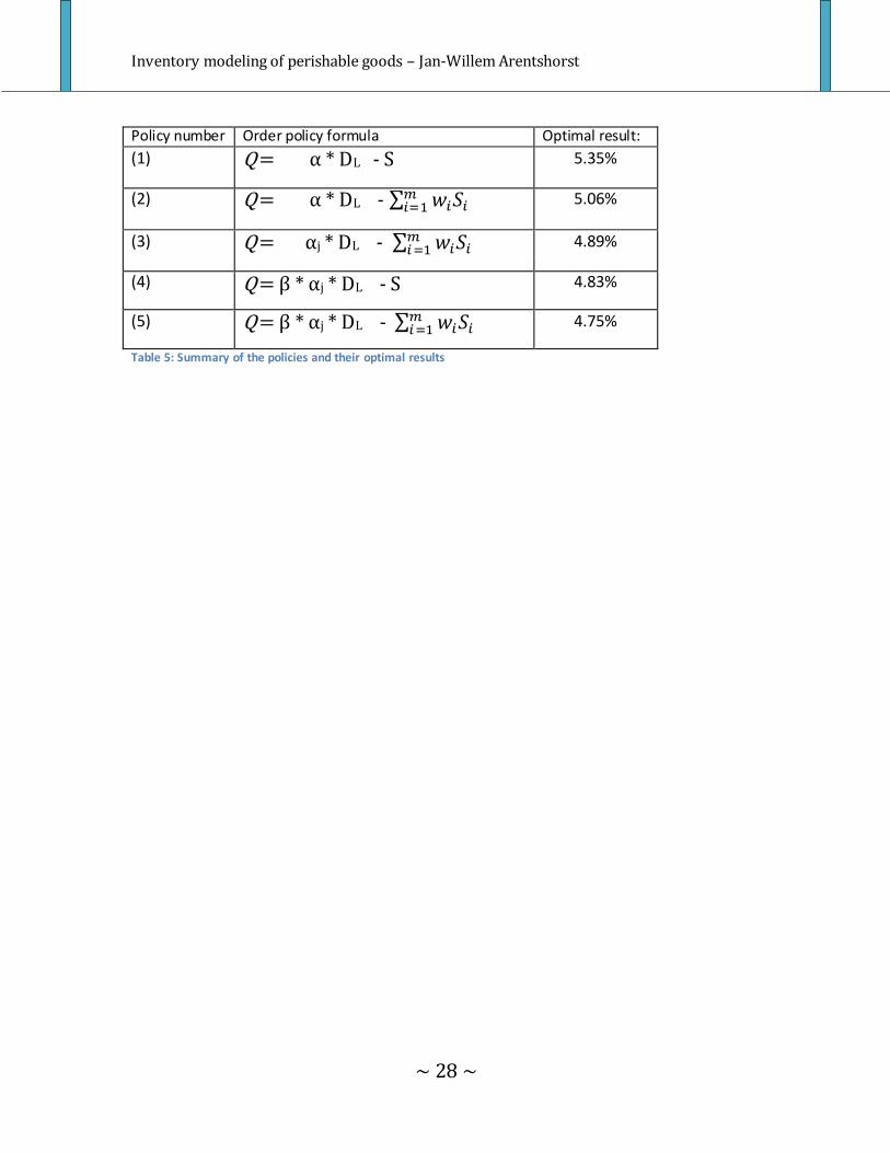
An overview of all policies, their formulas and best results for the standard settings is shown below in table 5.
Inventory modeling of perishable goods – Jan-Willem Arentshorst
~ 28 ~
Policy number Order policy formula Optimal result:
(1) Q = α * DL - S 5.35%
(2) Q = α * DL - 5.06%
(3) Q = αj * DL - 4.89%
(4) Q = β * αj * DL - S 4.83%
(5) Q = β * αj * DL - 4.75%
Table 5: Summary of the policies and their optimal results
Inventory modeling of perishable goods – Jan-Willem Arentshorst
~ 29 ~
7. Comparison to a real life situation
To compare the practical use of the model, information from a local s upermarket was
used to evaluate the order strategy. For a period of six weeks, stock levels, outdating, sales and deliveries for twelve different products were registered and afterwards
inserted into the computer program to compute how the order strategy would have scored in practice. The data was obtained from June 4th until July 15th 2011.
7.1 Supermarket information
The chosen supermarket is located in a Dutch village with approximately 15,000
inhabitants and has a weekly turnover of over €200,000. It is part of a multinational supermarket chain with a prominent position in the Dutch supermarket sector.
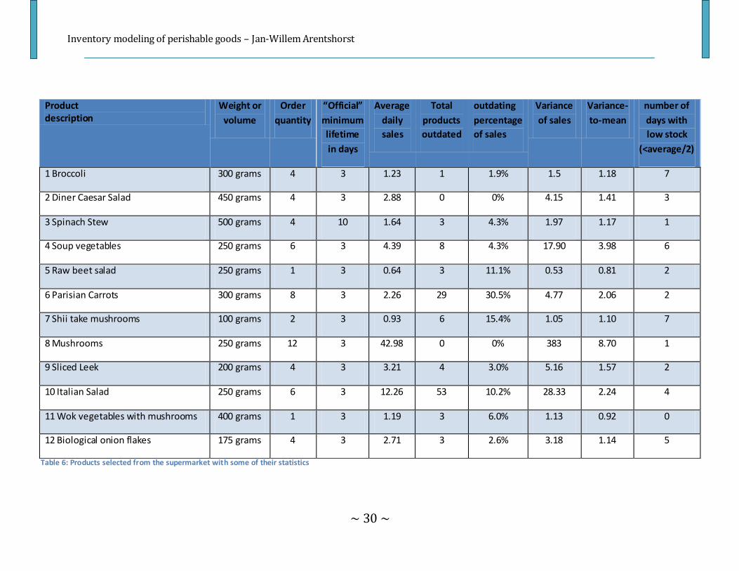
7.2 Product selection
A wide range of products was chosen, each with different average weekly sales and
minimum lifetime (d). In consultation with the local supermarket only products from the ready-to-cook vegetable department were chosen. The products in this department range from prepacked vegetables, like spinach and broccoli, to stir-fry vegetable mixes, mushrooms and prepacked lettuce and salads. This department is of interest because it is traditionally dealing with lots of outdating due to a rather short shelf life and has a somewhat larger profit margin than other products. A total of eighteen products were tracked, but not all could be used for the experiment, because during the interval, five
products were on sale. This dramatically boosted sales that week, which is not incorporated in the model and makes forecasting and parameter estimation even more
delicate. Furthermore, one product became unavailable due to shortages at the distribution centre. In the end, twelve products which are shown in table 6, were left for the real life analysis. It should be noted that the precision of the stated “minimum lifetime in days” is not accurate. This value was obtained from the computer system but it is not very accurate. For instance, the Parisian Carrots are supposed to last a minimum of 3 days, but as the data set shows, carrots arriving Friday evening are not thrown away until Thursday, which is five and a half to six days after arrival. Therefore, a sample was taken from the supermarket to obtain the correct life times. In nearly all cases, the expected life time after delivery was five days instead of three, except for the Spinach Stew which did last ten days. In the simulation, the “sampled” life times were used instead of the “official”
life times.
Inventory modeling of perishable goods – Jan-Willem Arentshorst
~ 30 ~
Product description
Weight or
volume
Order
quantity
“Official”
minimum
lifetime
in days
Average
daily
sales
Total
products
outdated
outdating
percentage
of sales
Variance
of sales
Variance-
to-mean
number of
days with
low stock
(<average/2)
1 Broccoli 300 grams 4 3 1.23 1 1.9% 1.5 1.18 7
2 Diner Caesar Salad 450 grams 4 3 2.88 0 0% 4.15 1.41 3
3 Spinach Stew 500 grams 4 10 1.64 3 4.3% 1.97 1.17 1
4 Soup vegetables 250 grams 6 3 4.39 8 4.3% 17.90 3.98 6
5 Raw beet salad 250 grams 1 3 0.64 3 11.1% 0.53 0.81 2
6 Parisian Carrots 300 grams 8 3 2.26 29 30.5% 4.77 2.06 2
7 Shii take mushrooms 100 grams 2 3 0.93 6 15.4% 1.05 1.10 7
8 Mushrooms 250 grams 12 3 42.98 0 0% 383 8.70 1
9 Sliced Leek 200 grams 4 3 3.21 4 3.0% 5.16 1.57 2
10 Italian Salad 250 grams 6 3 12.26 53 10.2% 28.33 2.24 4
11 Wok vegetables with mushrooms 400 grams 1 3 1.19 3 6.0% 1.13 0.92 0
12 Biological onion flakes 175 grams 4 3 2.71 3 2.6% 3.18 1.14 5
Table 6: Products selected from the supermarket with some of their statistics
Inventory modeling of perishable goods – Jan-Willem Arentshorst
~ 31 ~
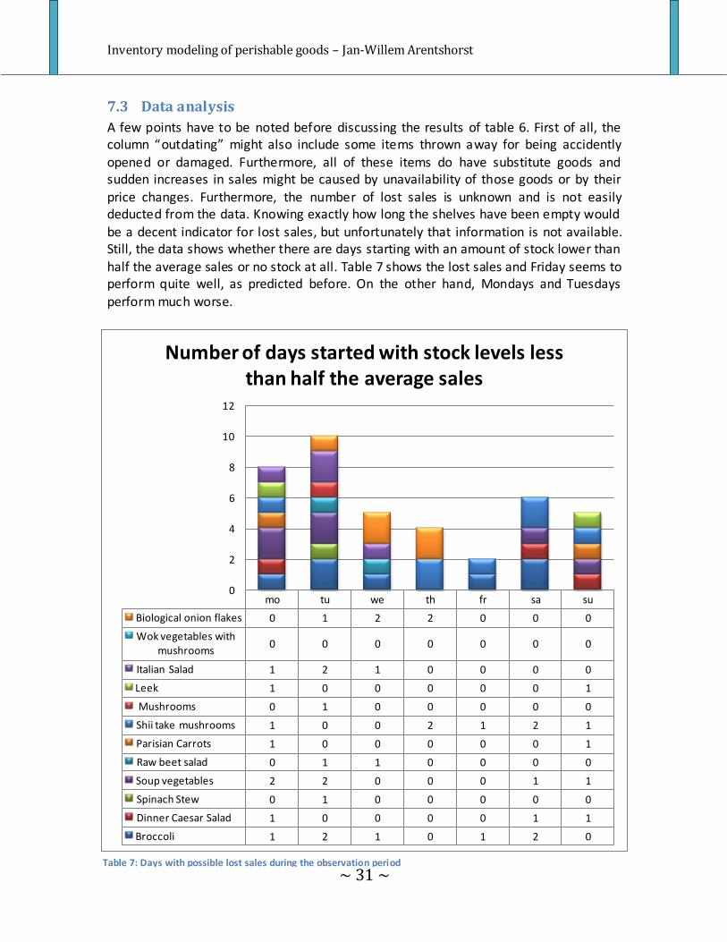
7.3 Data analysis
A few points have to be noted before discussing the results of table 6. First of all, the column “outdating” might also include some items thrown away for being accidently opened or damaged. Furthermore, all of these items do have substitute goods and sudden increases in sales might be caused by unavailability of those goods or by their price changes. Furthermore, the number of lost sales is unknown and is not easily deducted from the data. Knowing exactly how long the shelves have been empty would
be a decent indicator for lost sales, but unfortunately that information is not available. Still, the data shows whether there are days starting with an amount of stock lower than
half the average sales or no stock at all. Table 7 shows the lost sales and Friday seems to perform quite well, as predicted before. On the other hand, Mondays and Tuesdays
perform much worse.
mo tu we th fr sa su
Biological onion flakes 0 1 2 2 0 0 0
Wok vegetables with mushrooms
0 0 0 0 0 0 0
Italian Salad 1 2 1 0 0 0 0
Leek 1 0 0 0 0 0 1
Mushrooms 0 1 0 0 0 0 0
Shii take mushrooms 1 0 0 2 1 2 1
Parisian Carrots 1 0 0 0 0 0 1
Raw beet salad 0 1 1 0 0 0 0
Soup vegetables 2 2 0 0 0 1 1
Spinach Stew 0 1 0 0 0 0 0
Dinner Caesar Salad 1 0 0 0 0 1 1
Broccoli 1 2 1 0 1 2 0
0
2
4
6
8
10
12
Number of days started with stock levels less than half the average sales
Table 7: Days with possible lost sales during the observation period
Inventory modeling of perishable goods – Jan-Willem Arentshorst
~ 32 ~
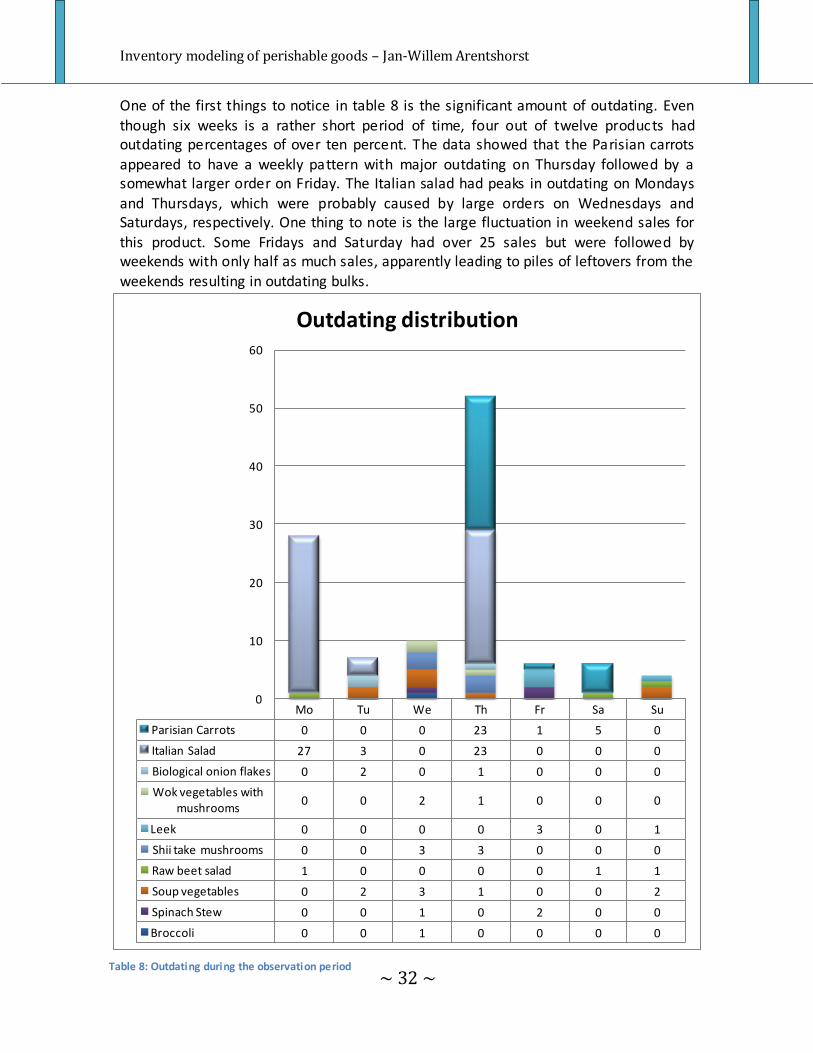
One of the first things to notice in table 8 is the significant amount of outdating. Even
though six weeks is a rather short period of time, four out of twelve products had outdating percentages of over ten percent. The data showed that the Parisian carrots
appeared to have a weekly pattern with major outdating on Thursday followed by a somewhat larger order on Friday. The Italian salad had peaks in outdating on Mondays
and Thursdays, which were probably caused by large orders on Wednesdays and Saturdays, respectively. One thing to note is the large fluctuation in weekend sales for
this product. Some Fridays and Saturday had over 25 sales but were followed by weekends with only half as much sales, apparently leading to piles of leftovers from the weekends resulting in outdating bulks.
Mo Tu We Th Fr Sa Su
Parisian Carrots 0 0 0 23 1 5 0
Italian Salad 27 3 0 23 0 0 0
Biological onion flakes 0 2 0 1 0 0 0
Wok vegetables with mushrooms
0 0 2 1 0 0 0
Leek 0 0 0 0 3 0 1
Shii take mushrooms 0 0 3 3 0 0 0
Raw beet salad 1 0 0 0 0 1 1
Soup vegetables 0 2 3 1 0 0 2
Spinach Stew 0 0 1 0 2 0 0
Broccoli 0 0 1 0 0 0 0
0
10
20
30
40
50
60
Outdating distribution
Table 8: Outdating during the observation period
Inventory modeling of perishable goods – Jan-Willem Arentshorst
~ 33 ~
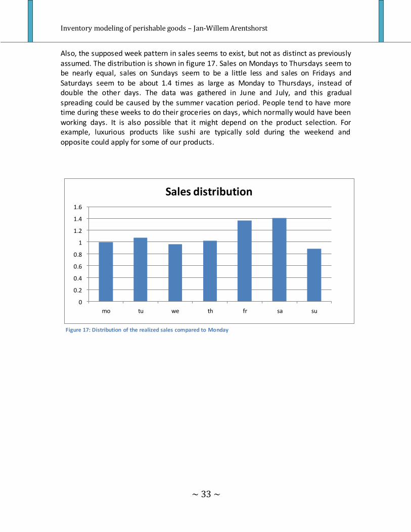
Also, the supposed week pattern in sales seems to exist, but not as distinct as previously
assumed. The distribution is shown in figure 17. Sales on Mondays to Thursdays seem to be nearly equal, sales on Sundays seem to be a little less and sales on Fridays and
Saturdays seem to be about 1.4 times as large as Monday to Thursdays, instead of double the other days. The data was gathered in June and July, and this gradual
spreading could be caused by the summer vacation period. People tend to have more time during these weeks to do their groceries on days, which normally would have been
working days. It is also possible that it might depend on the product selection. For example, luxurious products like sushi are typically sold during the weekend and opposite could apply for some of our products.
0
0.2
0.4
0.6
0.8
1
1.2
1.4
1.6
mo tu we th fr sa su
Sales distribution
Figure 17: Distribution of the realized sales compared to Monday
Inventory modeling of perishable goods – Jan-Willem Arentshorst
~ 34 ~
8. Simulation results compared to the real life situation
8.1 Settings and assumptions
Simulations were run using the store’s data to see if the strategies mentioned in chapter 4 perform properly. The data comprises a total of six weeks. We simulated cycles of 42
days, and did this for each product 100,000 times to obtain accurate results. One should note that we have a significant advantage since the realization of the demand is already
known, whereas the store had to estimate it using historic data of hundreds of stores throughout the Netherlands.
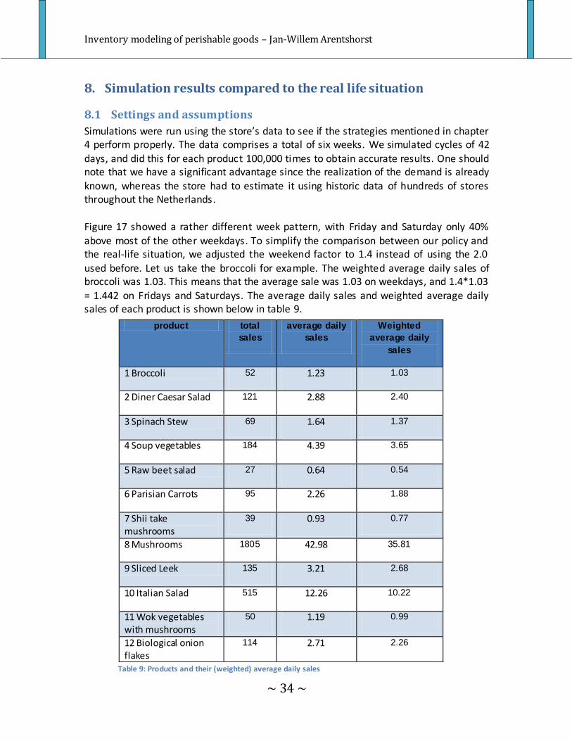
Figure 17 showed a rather different week pattern, with Friday and Saturday only 40%
above most of the other weekdays. To simplify the comparison between our policy and the real-life situation, we adjusted the weekend factor to 1.4 instead of using the 2.0
used before. Let us take the broccoli for example. The weighted average daily sales of broccoli was 1.03. This means that the average sale was 1.03 on weekdays, and 1.4*1.03 = 1.442 on Fridays and Saturdays. The average daily sales and weighted average daily sales of each product is shown below in table 9.
Table 9: Products and their (weighted) average daily sales
product total
sales
average daily
sales
Weighted
average daily
sales
1 Broccoli 52 1.23 1.03
2 Diner Caesar Salad 121 2.88 2.40
3 Spinach Stew 69 1.64 1.37
4 Soup vegetables 184 4.39 3.65
5 Raw beet salad 27 0.64 0.54
6 Parisian Carrots 95 2.26 1.88
7 Shii take mushrooms
39 0.93 0.77
8 Mushrooms 1805 42.98 35.81
9 Sliced Leek 135 3.21 2.68
10 Italian Salad 515 12.26 10.22
11 Wok vegetables with mushrooms
50 1.19 0.99
12 Biological onion flakes
114 2.71 2.26
Inventory modeling of perishable goods – Jan-Willem Arentshorst
~ 35 ~
Using the results from table 8 as input variables, simulations were carried out for each
of the specified products. The supermarket had a certain stock build-up at the begin of the measurements. The age distribution of the stock was unknown, but has a significant
effect on simulation results. Starting with a clean sheet, i.e. entirely young stock, makes it easier for the system to keep outdating to a minimum than if the stock was randomly
divided over all stock ages. Each simulation cycle starts with the same pre-specified amount of initial stock. The age distribution of the stock at the start of a new cycle is
made to resemble the age distribution at the end of the previous cycle. Otherwise, the system would always start out with only fully fresh items, which would not be realistic. For the comparison, the forth policy was used, since this thesis is mainly interested in a practical policy and this policy does not use ‘uncommon’ information like the age distribution of the actual stock. The policy is given by:
Q = β * αj * DL - S , (4) where αj and β were optimized by simulation.
8.2 Comparison on lost sales
Since no information is known about lost sales in the supermarket, we use ‘the number of days with rather low stock’ as a performance measure. The number of days were counted on which the stock at the start of the day was less than half the expected sales of that day. Although it does not give an indication of the total number of lost sales, it does give some insight in how frequent orders are insufficient. We cannot compare our policy with the supermarket using the sum of the percentage of outdating and of lost sales, since we have no information on the amount of outdating. What we can do is fixing one of the two values and determine if our policy performs better. So the
simulated policy tries to accomplish approximately the same number of days with low stock, but with less outdating.
Table 10 shows the comparison between de supermarket and our simulations.
Especially the Parisian Carrots (6) and the Shii take Mushrooms (7) did far better than in practice. The four products listed in red in table 10 are the ones in which our policy
performs worse. Note that the required alpha to match the supermarket is less than one for the Soup vegetables (4), Mushrooms (8) and Italian Salad (10). This means they actually deliberately have lost sales to match the low stock levels, which obviously
decreases the outdating percentages. In real life, this is obviously never an optimal solution. One of the reasons why the mushrooms achieved such low outdating rates is
that they are placed on the bottom shelf in a corner, which makes it very hard for customers not to buy FIFO, achieving no outdating at all. The Italian salad had rather full
shelves but had terrible outdating as can be seen in table 10. This might be caused by an incorrect administrative stock level, i.e. the system contained more products than it
knew about, which rarely happens.

Inventory modeling of perishable goods – Jan-Willem Arentshorst
~ 36 ~
Product description
Realized low
stock in days
Simulated low
stock in days
Realized
outdating
Simulated
Outdating
Simulated
Lost sales
Optimal
alpha
1 Broccoli 7 6.97 1.9% 4.18% 25.15% 1.28
2 Diner Caesar Salad 3 3.31 0% 1.22% 13.81% 1.2
3 Spinach Stew 1 1.2 4.3% 0.62% 8.94% 1.66
4 Soup vegetables 6 6.19 4.3% 0.46% 26.79% 0.98
5 Raw beet salad 2 2.31 11.1% 16.07% 10.76% 2.04
6 Parisian Carrots 2 2.47 30.5% 7.02% 12.80% 1.7
7 Shii take mushrooms 7 6 15.4% 4.94% 25.82% 1.19
8 Mushrooms 1 0.54 0% 0% 51.52% 0.47
9 Sliced Leek 2 2.16 3.0% 1.09% 12.67% 1.19
10 Italian Salad 4 3.68 10.2% 0% 49.46% 0.45
11 Wok vegetables with
mushrooms 0 0.44 6.0% 9.45% 6.72% 1.75
12 Biological onion flakes 5 5.36 2.6% 0.77% 21.63% 1.17
Table 10: Comparison between the supermarket and simulation for a fixed amount of low stock
Inventory modeling of perishable goods – Jan-Willem Arentshorst
~ 37 ~
8.3 Comparison on outdating
The same comparison was done with outdating. Similar to the previous section, we fixed the amount of outdating and compared the difference in days with low stock. The five products colored red are the ones in which our policy performs worse. Table 11 shows that seven out of twelve items would have performed better using our
policy. Note that the alpha of the first two products are below one. Especially the broccoli results were difficult to obtain, since it has a rather low average daily sales and
it is very hard to keep outdating to a minimum under our assumptions of not-fully FIFO. That is why the simulated lost sales are so high for that product. One of the reasons why
the other ‘red’ products performed so well is that the supermarket had an active policy giving a significant discount to all items with one day until expiry, actively increasing the chance customers will take an old item over a younger one.
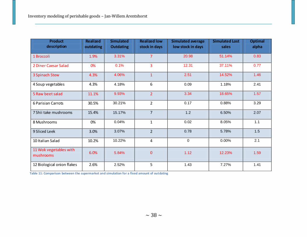
Inventory modeling of perishable goods – Jan-Willem Arentshorst
~ 38 ~
Table 11: Comparison between the supermarket and simulation for a fixed amount of outdating
Product description
Realized
outdating
Simulated
Outdating
Realized low
stock in days
Simulated average
low stock in days
Simulated Lost
sales
Optimal
alpha
1 Broccoli 1.9% 3.31% 7 20.98 51.14% 0.83
2 Diner Caesar Salad 0% 0.1% 3 12.31 37.11% 0.77
3 Spinach Stew 4.3% 4.06% 1 2.51 14.52% 1.46
4 Soup vegetables 4.3% 4.18% 6 0.09 1.18% 2.41
5 Raw beet salad 11.1% 9.93% 2 3.34 18.65% 1.57
6 Parisian Carrots 30.5% 30.21% 2 0.17 0.88% 3.29
7 Shii take mushrooms 15.4% 15.17% 7 1.2 6.50% 2.07
8 Mushrooms 0% 0.04% 1 0.02 8.05% 1.1
9 Sliced Leek 3.0% 3.07% 2 0.78 5.78% 1.5
10 Italian Salad 10.2% 10.22% 4 0 0.00% 2.1
11 Wok vegetables with
mushrooms 6.0% 5.84% 0 1.12 12.23% 1.59
12 Biological onion flakes 2.6% 2.52% 5 1.43 7.27% 1.41
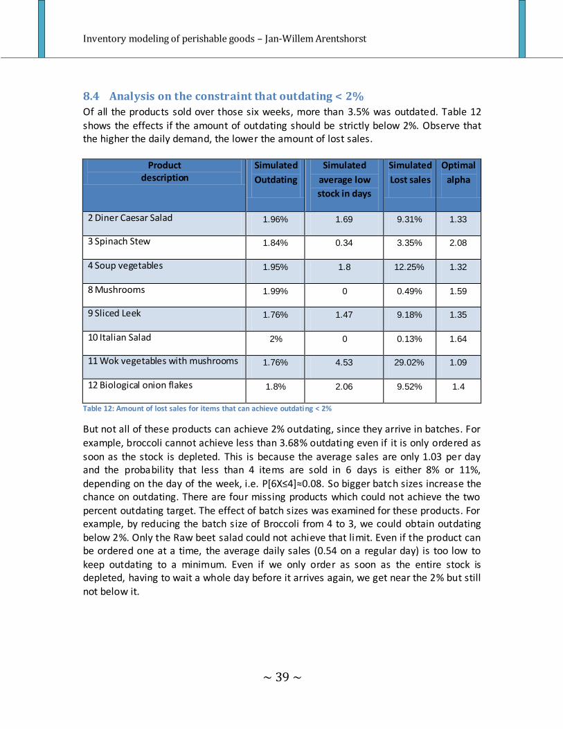
Inventory modeling of perishable goods – Jan-Willem Arentshorst
~ 39 ~
8.4 Analysis on the constraint that outdating < 2%
Of all the products sold over those six weeks, more than 3.5% was outdated. Table 12 shows the effects if the amount of outdating should be strictly below 2%. Observe that the higher the daily demand, the lower the amount of lost sales.
Product description
Simulated
Outdating
Simulated
average low
stock in days
Simulated
Lost sales
Optimal
alpha
2 Diner Caesar Salad 1.96% 1.69 9.31% 1.33
3 Spinach Stew 1.84% 0.34 3.35% 2.08
4 Soup vegetables 1.95% 1.8 12.25% 1.32
8 Mushrooms 1.99% 0 0.49% 1.59
9 Sliced Leek 1.76% 1.47 9.18% 1.35
10 Italian Salad 2% 0 0.13% 1.64
11 Wok vegetables with mushrooms 1.76% 4.53 29.02% 1.09
12 Biological onion flakes 1.8% 2.06 9.52% 1.4
Table 12: Amount of lost sales for items that can achieve outdating < 2%
But not all of these products can achieve 2% outdating, since they arrive in batches. For example, broccoli cannot achieve less than 3.68% outdating even if it is only ordered as
soon as the stock is depleted. This is because the average sales are only 1.03 per day and the probability that less than 4 items are sold in 6 days is either 8% or 11%,
depending on the day of the week, i.e. P[6X≤4]≈0.08. So bigger batch sizes increase the chance on outdating. There are four missing products which could not achieve the two percent outdating target. The effect of batch sizes was examined for these products. For example, by reducing the batch size of Broccoli from 4 to 3, we could obtain outdating below 2%. Only the Raw beet salad could not achieve that limit. Even if the product can be ordered one at a time, the average daily sales (0.54 on a regular day) is too low to keep outdating to a minimum. Even if we only order as soon as the entire stock is depleted, having to wait a whole day before it arrives again, we get near the 2% but still not below it.
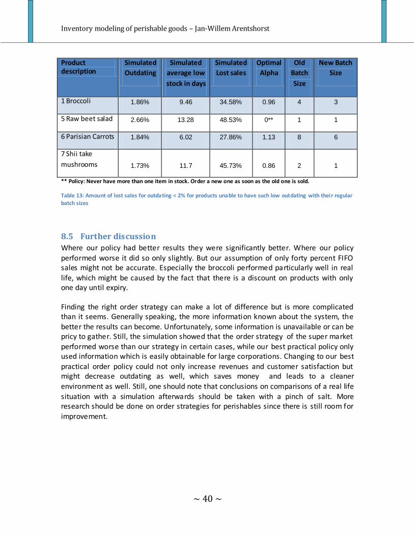
Inventory modeling of perishable goods – Jan-Willem Arentshorst
~ 40 ~
Product description
Simulated
Outdating
Simulated
average low
stock in days
Simulated
Lost sales
Optimal
Alpha
Old
Batch
Size
New Batch
Size
1 Broccoli 1.86% 9.46 34.58% 0.96 4 3
5 Raw beet salad 2.66% 13.28 48.53% 0** 1 1
6 Parisian Carrots 1.84% 6.02 27.86% 1.13 8 6
7 Shii take
mushrooms 1.73% 11.7 45.73% 0.86 2 1
** Policy: Never have more than one item in stock. Order a new one as soon as the old one is sold.
Table 13: Amount of lost sales for outdating < 2% for products unable to have such low outdating with their regular batch sizes
8.5 Further discussion
Where our policy had better results they were significantly better. Where our policy
performed worse it did so only slightly. But our assumption of only forty percent FIFO sales might not be accurate. Especially the broccoli performed particularly well in real
life, which might be caused by the fact that there is a discount on products with only one day until expiry.
Finding the right order strategy can make a lot of difference but is more complicated than it seems. Generally speaking, the more information known about the system, the better the results can become. Unfortunately, some information is unavailable or can be pricy to gather. Still, the simulation showed that the order strategy of the super market performed worse than our strategy in certain cases, while our best practical policy only used information which is easily obtainable for large corporations. Changing to our best
practical order policy could not only increase revenues and customer satisfaction but might decrease outdating as well, which saves money and leads to a cleaner
environment as well. Still, one should note that conclusions on comparisons of a real life situation with a simulation afterwards should be taken with a pinch of salt. More research should be done on order strategies for perishables since there is still room for improvement.
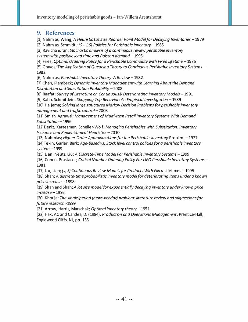
Inventory modeling of perishable goods – Jan-Willem Arentshorst
~ 41 ~
9. References [1] Nahmias, Wang; A Heuristic Lot Size Reorder Point Model for Decaying Inventories – 1979 [2] Nahmias, Schmidtl; (S - 1,S) Policies for Perishable Inventory – 1985 [3] Ravichandran; Stochastic analysis of a continuous review perishable inventory system with positive lead time and Poisson demand – 1995 [4] Fries; Optimal Ordering Policy for a Perishable Commodity with Fixed Lifetime – 1975 [5] Graves; The Application of Queueing Theory to Continuous Perishable Inventory Systems – 1982 [6] Nahmias; Perishable Inventory Theory: A Review – 1982 [7] Chen, Plambeck; Dynamic Inventory Management with Learning About the Demand Distribution and Substitution Probability – 2008 [8] Raafat; Survey of Literature on Continuously Deteriorating Inventory Models – 1991 [9] Kahn, Schmittlein; Shopping Trip Behavior: An Empirical Investigation – 1989 [10] Haijema; Solving large structured Markov Decision Problems for perishable inventory management and traffic control – 2008 [11] Smith, Agrawal; Management of Multi-Item Retail Inventory Systems With Demand Substitution – 1996 [12]Deniz, Karaesmen, Scheller-Wolf; Managing Perishables with Substitution: Inventory Issuance and Replenishment Heuristics – 2010 [13] Nahmias; Higher-Order Approximations for the Perishable-Inventory Problem – 1977 [14]Tekin, Gurler, Berk; Age-Based vs. Stock level control policies for a perishable inventory system – 1999 [15] Lian, Neuts, Liu; A Discrete-Time Model For Perishable Inventory Systems – 1999 [16] Cohen, Prastacos; Critical Number Ordering Policy For LIFO Perishable Inventory Systems – 1981 [17] Liu, Lian; (s, S) Continuous Review Models for Products With Fixed Lifetimes – 1995 [18] Shah; A discrete-time probabilistic inventory model for deteriorating items under a known price increase – 1998 [19] Shah and Shah; A lot size model for exponentially decaying inventory under known price increase – 1993 [20] Khouja; The single-period (news-vendor) problem: literature review and suggestions for future research -1999 [21] Arrow, Harris, Marschak; Optimal inventory theory – 1951 [22] Hax, AC and Candea, D. (1984), Production and Operations Management, Prentice-Hall, Englewood Cliffs, NJ, pp. 135
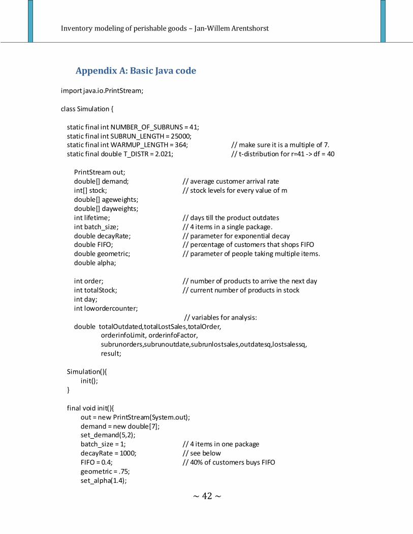
Inventory modeling of perishable goods – Jan-Willem Arentshorst
~ 42 ~
Appendix A: Basic Java code import java.io.PrintStream; class Simulation { static final int NUMBER_OF_SUBRUNS = 41; static final int SUBRUN_LENGTH = 25000; static final int WARMUP_LENGTH = 364; // make sure it is a multiple of 7. static final double T_DISTR = 2.021; // t-distribution for r=41 -> df = 40 PrintStream out; double[] demand; // average customer arrival rate int[] stock; // stock levels for every value of m double[] ageweights; double[] dayweights; int lifetime; // days till the product outdates int batch_size; // 4 items in a single package. double decayRate; // parameter for exponential decay double FIFO; // percentage of customers that shops FIFO double geometric; // parameter of people taking multiple items. double alpha; int order; // number of products to arrive the next day int totalStock; // current number of products in stock int day; int lowordercounter; // variables for analysis: double totalOutdated,totalLostSales,totalOrder, orderinfoLimit, orderinfoFactor, subrunorders,subrunoutdate,subrunlostsales,outdatesq,lostsalessq, result; Simulation(){ init(); } final void init(){ out = new PrintStream(System.out); demand = new double[7]; set_demand(5,2); batch_size = 1; // 4 items in one package decayRate = 1000; // see below FIFO = 0.4; // 40% of customers buys FIFO geometric = .75; set_alpha(1.4);
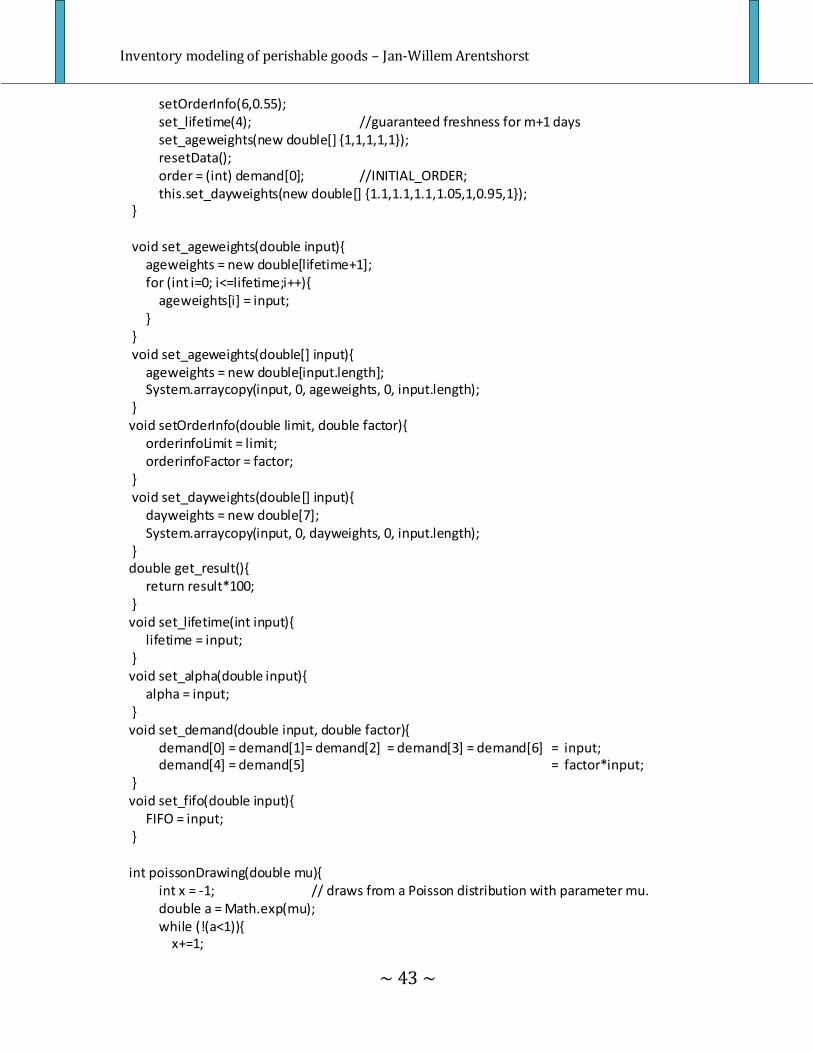
Inventory modeling of perishable goods – Jan-Willem Arentshorst
~ 43 ~
setOrderInfo(6,0.55); set_lifetime(4); //guaranteed freshness for m+1 days set_ageweights(new double[] {1,1,1,1,1}); resetData(); order = (int) demand[0]; //INITIAL_ORDER; this.set_dayweights(new double[] {1.1,1.1,1.1,1.05,1,0.95,1}); } void set_ageweights(double input){ ageweights = new double[lifetime+1]; for (int i=0; i<=lifetime;i++){ ageweights[i] = input; } } void set_ageweights(double[] input){ ageweights = new double[input.length]; System.arraycopy(input, 0, ageweights, 0, input.length); } void setOrderInfo(double limit, double factor){ orderinfoLimit = limit; orderinfoFactor = factor; } void set_dayweights(double[] input){ dayweights = new double[7]; System.arraycopy(input, 0, dayweights, 0, input.length); } double get_result(){ return result*100; } void set_lifetime(int input){ lifetime = input; } void set_alpha(double input){ alpha = input; } void set_demand(double input, double factor){ demand[0] = demand[1]= demand[2] = demand[3] = demand[6] = input; demand[4] = demand[5] = factor*input; } void set_fifo(double input){ FIFO = input; } int poissonDrawing(double mu){ int x = -1; // draws from a Poisson distribution with parameter mu. double a = Math.exp(mu); while (!(a<1)){ x+=1;
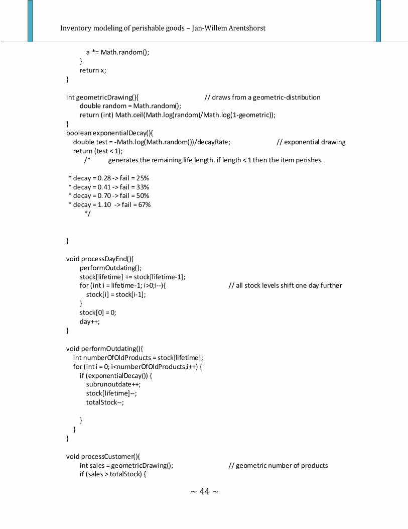
Inventory modeling of perishable goods – Jan-Willem Arentshorst
~ 44 ~
a *= Math.random(); } return x; } int geometricDrawing(){ // draws from a geometric-distribution double random = Math.random(); return (int) Math.ceil(Math.log(random)/Math.log(1-geometric)); } boolean exponentialDecay(){ double test = -Math.log(Math.random())/decayRate; // exponential drawing return (test < 1);
/* generates the remaining life length. if length < 1 then the item perishes. * decay = 0.28 -> fail = 25% * decay = 0.41 -> fail = 33% * decay = 0.70 -> fail = 50% * decay = 1.10 -> fail = 67% */ } void processDayEnd(){ performOutdating(); stock[lifetime] += stock[lifetime-1]; for (int i = lifetime-1; i>0;i--){ // all stock levels shift one day further stock[i] = stock[i-1]; } stock[0] = 0; day++; } void performOutdating(){ int numberOfOldProducts = stock[lifetime]; for (int i = 0; i<numberOfOldProducts;i++) { if (exponentialDecay()) { subrunoutdate++; stock[lifetime]--; totalStock--; } } } void processCustomer(){ int sales = geometricDrawing(); // geometric number of products if (sales > totalStock) {
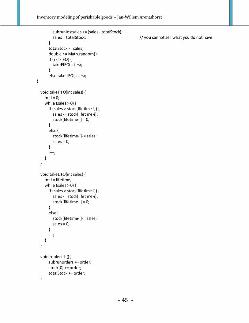
Inventory modeling of perishable goods – Jan-Willem Arentshorst
~ 45 ~
subrunlostsales += (sales - totalStock); sales = totalStock; // you cannot sell what you do not have } totalStock -= sales; double r = Math.random(); if (r < FIFO) { takeFIFO(sales); } else takeLIFO(sales); } void takeFIFO(int sales) { int i = 0; while (sales > 0) { if (sales > stock[lifetime-i]) { sales -= stock[lifetime-i]; stock[lifetime-i] = 0; } else { stock[lifetime-i]-= sales; sales = 0; } i++; } } void takeLIFO(int sales) { int i = lifetime; while (sales > 0) { if (sales > stock[lifetime-i]) { sales -= stock[lifetime-i]; stock[lifetime-i] = 0; } else { stock[lifetime-i]-= sales; sales = 0; } i--; } } void replenish(){ subrunorders += order; stock[0] += order; totalStock += order; }
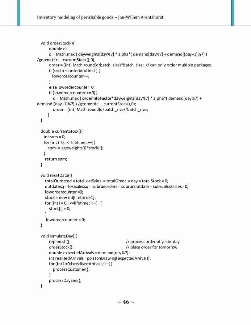
Inventory modeling of perishable goods – Jan-Willem Arentshorst
~ 46 ~
void orderStock(){ double d; d = Math.max ( dayweights[day%7] * alpha*( demand[day%7] + demand[(day+1)%7] ) /geometric - currentStock(),0); order = (int) Math.round(d/batch_size)*batch_size; // can only order multiple packages. if (order < orderinfoLimit ) { lowordercounter++; } else lowordercounter=0; if (lowordercounter >= 3){ d = Math.max ( orderinfoFactor*dayweights[day%7] * alpha*( demand[day%7] + demand[(day+1)%7] ) /geometric - currentStock(),0); order = (int) Math.round(d/batch_size)*batch_size; } } double currentStock(){ int som = 0; for (int i=0; i<=lifetime;i++){ som+= ageweights[i]*stock[i]; } return som; } void resetData(){ totalOutdated = totalLostSales = totalOrder = day = totalStock = 0; outdatesq = lostsalessq = subrunorders = subrunoutdate = subrunlostsales= 0; lowordercounter =0; stock = new int[lifetime+1]; for (int i = 0; i<=lifetime; i++) { stock[i] = 0; } lowordercounter = 0; } void simulateDay(){ replenish(); // process order of yesterday orderStock(); // place order for tomorrow double expectedArrivals = demand[day%7]; int realisedArrivals= poissonDrawing(expectedArrivals); for (int i =0;i<realisedArrivals;i++){ processCustomer(); } processDayEnd(); }
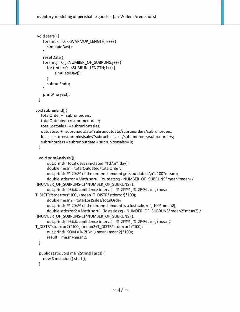
Inventory modeling of perishable goods – Jan-Willem Arentshorst
~ 47 ~
void start() { for (int k = 0; k<WARMUP_LENGTH; k++) { simulateDay(); } resetData(); for (int j = 0; j<NUMBER_OF_SUBRUNS;j++) { for (int i = 0; i<SUBRUN_LENGTH; i++) { simulateDay(); } subrunEnd(); } printAnalysis(); } void subrunEnd(){ totalOrder += subrunorders; totalOutdated += subrunoutdate; totalLostSales += subrunlostsales; outdatesq += subrunoutdate*subrunoutdate/subrunorders/subrunorders; lostsalessq +=subrunlostsales*subrunlostsales/subrunorders/subrunorders; subrunorders = subrunoutdate = subrunlostsales= 0; } void printAnalysis(){ out.printf("Total days simulated: %d.\n", day); double mean = totalOutdated/totalOrder; out.printf("%.2f%% of the ordered amount gets outdated.\n", 100*mean); double stderror = Math.sqrt( (outdatesq - NUMBER_OF_SUBRUNS*mean*mean) / ((NUMBER_OF_SUBRUNS-1)*NUMBER_OF_SUBRUNS) ); out.printf("95%% confidence interval: %.2f%% , %.2f%% .\n", (mean-T_DISTR*stderror)*100 , (mean+T_DISTR*stderror)*100); double mean2 = totalLostSales/totalOrder; out.printf("%.2f%% of the ordered amount is a lost sale.\n", 100*mean2); double stderror2 = Math.sqrt( (lostsalessq - NUMBER_OF_SUBRUNS*mean2*mean2) / ((NUMBER_OF_SUBRUNS-1)*NUMBER_OF_SUBRUNS) ); out.printf("95%% confidence interval: %.2f%% , %.2f%% .\n", (mean2-T_DISTR*stderror2)*100 , (mean2+T_DISTR*stderror2)*100); out.printf("SOM = %.2f \n",(mean+mean2)*100); result = mean+mean2; } public static void main(String[] args) { new Simulation().start(); }
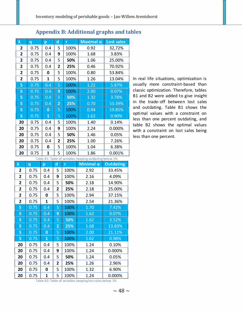
Inventory modeling of perishable goods – Jan-Willem Arentshorst
~ 48 ~
Appendix B: Additional graphs and tables
In real life situations, optimization is usually more constraint-based than
classic optimization. Therefore, tables B1 and B2 were added to give insight
in the trade-off between lost sales and outdating. Table B1 shows the
optimal values with a constraint on less than one percent outdating, and table B2 shows the optimal values with a constraint on lost sales being less than one percent.
Table B1: Table of variables keeping outdating below 1%
λ q p d r Minimal α Outdating
2 0.75 0.4 5 100% 2.92 33.45%
2 0.75 0.4 9 100% 2.16 4.09%
2 0.75 0.4 5 50% 2.18 14.90%
2 0.75 0.4 2 25% 2.18 25.00%
2 0.75 0 5 100% 2.94 37.15%
2 0.75 1 5 100% 2.54 21.36%
5 0.75 0.4 5 100% 1.70 7.42%
5 0.75 0.4 9 100% 1.62 0.07%
5 0.75 0.4 5 50% 1.62 3.52%
5 0.75 0.4 2 25% 1.68 13.83%
5 0.75 0 5 100% 2.00 21.11%
5 0.75 1 5 100% 1.62 0.98%
20 0.75 0.4 5 100% 1.24 0.10% 20 0.75 0.4 9 100% 1.24 0.000%
20 0.75 0.4 5 50% 1.24 0.05%
20 0.75 0.4 2 25% 1.26 2.96%
20 0.75 0 5 100% 1.32 6.90%
20 0.75 1 5 100% 1.24 0.000% Table B2: Table of variables keeping lost sales below 1%
λ q p d r Maximal α Lost sales
2 0.75 0.4 5 100% 0.92 32,72% 2 0.75 0.4 9 100% 1.68 3.83%
2 0.75 0.4 5 50% 1.06 25.00%
2 0.75 0.4 2 25% 0.46 70.92%
2 0.75 0 5 100% 0.80 53.84%
2 0.75 1 5 100% 1.26 13.04%
5 0.75 0.4 5 100% 1.22 5.87%
5 0.75 0.4 9 100% 2.00 0.07% 5 0.75 0.4 5 50% 1.32 3.78%
5 0.75 0.4 2 25% 0.70 53.39%
5 0.75 0 5 100% 0.94 19.85%
5 0.75 1 5 100% 1.62 0.90%
20 0.75 0.4 5 100% 1.40 0.14%
20 0.75 0.4 9 100% 2.24 0.000%
20 0.75 0.4 5 50% 1.46 0.05%
20 0.75 0.4 2 25% 1.00 7.26% 20 0.75 0 5 100% 1.04 6.38%
20 0.75 1 5 100% 1.86 0.001%