Inverse modelling for predicting bothwater and nitrate movement in astructured-clay soil (Red Ferrosol)James M. Kirkham1, Christopher J. Smith2, Richard B. Doyle1 andPhilip H. Brown3

1 Tasmanian Institute of Agriculture, University of Tasmania, Hobart, TAS, Australia2 Land and Water, CSIRO, Canberra, ACT, Australia3 Centre for Plant and Water Science, Central Queensland University, Bundaberg, QLD, Australia

ABSTRACTSoil physical parameter calculation by inverse modelling provides an indirectway of estimating the unsaturated hydraulic properties of soils. However manymeasurements are needed to provide sufficient data to determine unknownparameters. The objective of this research was to assess the use of unsaturated waterflow and solute transport experiments, in horizontal packed soil columns, toestimate the parameters that govern water flow and solute transport. The derivedparameters are then used to predict water infiltration and solute migration in arepacked soil wedge. Horizontal columns packed with Red Ferrosol were used in anitrate diffusion experiment to estimate either three or six parameters of the vanGenuchten–Mualem equation while keeping residual and saturated water content,and saturated hydraulic conductivity fixed to independently measured values.These parameters were calculated using the inverse optimisation routines inHydrus 1D. Nitrate concentrations measured along the horizontal soil columns wereused to independently determine the Langmuir adsorption isotherm. The soilhydraulic properties described by the van Genuchten–Mualem equation, and theNO3

– adsorption isotherm, were then used to predict water and NO3– distributions

from a point-source in two 3D flow scenarios. The use of horizontal columnsof repacked soil and inverse modelling to quantify the soil water retentioncurve was found to be a simple and effective method for determining soil hydraulicproperties of Red Ferrosols. These generated parameters supported subsequenttesting of interactive flow and reactive transport processes under dynamicflow conditions.

Subjects Agricultural Science, Soil Science, Environmental ImpactsKeywords Pedotransfer functions, Water flow, Rosetta, Hydrus, Soil water, Nitrate, Hydrus-1D,Hydrus-2D

INTRODUCTIONSimulation models are useful for examining water and solute movement in soil profiles,such as when improving water and nutrient use efficiency or designing fertigation systems(Cote et al., 2003; Skaggs et al., 2004; Siyal & Skaggs, 2009). There are a number ofsoil water models, such as LeachM (Wagenet & Hutson, 1989), Wet-Up (Cook et al., 2003),

How to cite this article Kirkham JM, Smith CJ, Doyle RB, Brown PH. 2019. Inverse modelling for predicting both water and nitratemovement in a structured-clay soil (Red Ferrosol). PeerJ 6:e6002 DOI 10.7717/peerj.6002

Submitted 30 March 2018Accepted 25 October 2018Published 16 January 2019

Corresponding authorRichard B. Doyle,Richard.Doyle@utas.edu.au

Academic editorSamuel Abiven

Additional Information andDeclarations can be found onpage 19

DOI 10.7717/peerj.6002

Copyright2019 Kirkham et al.

Distributed underCreative Commons CC-BY 4.0

Hydrus 1D (Šimůnek et al., 2008), Hydrus 2D/3D (Šimůnek, Van Genuchten & Šejna,2006), and numerical procedures described by Wu & Chieng (1995a, 1995b) which are allcapable of describing water flow, and in some cases solute transport, in one, two, orthree dimensions. In this study, we selected the suite of Hydrus models, because they cansimulate solute flow under both 1D and 3D conditions. The van Genuchten–Mualemwater content, capillary pressure and hydraulic conductivity models were used to predictwater flow (Šimůnek, Van Genuchten & Šejna, 2006), but physically realistic parametersare needed for the intended application if accurate predictions are to be made.

Inverse optimisation techniques have become increasingly popular for parameterestimation and many soil models now have user-friendly optimisation tools built in(Hopmans et al., 2002; Vrugt & Bouten, 2002; Wöhling, Vrugt & Barkle, 2008; Kandelouset al., 2011). The method involves multiple calculations in which parameters areadjusted, using a method such as the Levenberg–Marquardt or Bayesian procedure, untilpredictions agree sufficiently well with the measured data (Šimůnek, Van Genuchten &Šejna, 2006). This has advantages over other techniques for estimating hydraulicparameters, such as pedotransfer functions (PTFs), because the optimised parameters areestimated directly from measured data for a particular soil hydrological problem ofinterest. Care however must be taken when using this method to ensure parameters arephysically realistic and representative of the spatial scale of interest (Hopmans et al., 2002;Vrugt & Bouten, 2002; Mallants et al., 2007; Wöhling, Vrugt & Barkle, 2008).

Šimůnek et al. (2000) used inverse optimisation to estimate soil hydraulic parametersfrom water content data measured in horizontal absorption columns. Similarly, inverseoptimisation has been used in Hydrus to predict water flow from water potential andcumulative outflow data (Van Dam, Stricker & Droogers, 1994; Hopmans et al., 2002;Arbat et al., 2008). Kandelous & Šimůnek (2010a, 2010b) and Kandelous et al. (2011) usedinverse optimisation to estimate soil hydraulic parameters to predict water distributionfrom a point source, including subsurface irrigation, in the field.Mallants et al. (2007) usedHydrus 2D and cumulative infiltration data from a deep borehole infiltration test in clayeygravel and carbonated loess soil to estimate field-scale soil hydraulic properties.

Despite the increasing popularity of inverse optimisation, there are few publishedexamples in which parameters derived from unsaturated flow absorption columns havebeen tested in 3D flow scenarios. Obtaining parameters for a specific flow scenariodoes not guarantee they will be suitable for extrapolation outside the measured data set towhich they were fitted (Sonnleitner, Abbaspour & Schulin, 2003). Vrugt & Bouten (2002)and Wöhling, Vrugt & Barkle (2008) recommend the use of the Metropolis algorithmto determine parameter uncertainty, given measurement errors and the models inability toperfectly represent the system. However, if the derived parameters can be shown to becapable of approximating the observed water content distribution under contrastingconditions, it is likely they are physically realistic for the conditions being investigated.To this end, Sonnleitner, Abbaspour & Schulin (2003) and Kandelous et al. (2011) usedinverse parameter estimation to improve simulations of water content data underdifferent flow scenarios. Minimising the number of optimised parameters, increases thelikelihood that the parameters are physically realistic (Hopmans et al., 2002).

Kirkham et al. (2019), PeerJ, DOI 10.7717/peerj.6002 2/23

Although several numerical models, including Hydrus (Hanson, Šimůnek & Hopmans,2006), have looked at reactive solute transport (Molinero et al., 2008; Kuntz &Grathwohl, 2009; Nakagawa et al., 2010), validation of the models has been limited.Phillips (2006) used Hydrus and some unpublished data to predict the transport of K+ inunsaturated repacked horizontal columns of reactive soil similar to the one used inthis study. In field-scale simulations using Hydrus 1D, Persicani (1995) and Moradi,Abbaspour & Afyuni (2005) had limited success in simulating reactive metal movementover extended time-scales. However, Rassam & Cook (2002) were able to use modelling ofsolute fluxes in soils to explain results from the field and laboratory measurements ofRassam, Cook & Gardner (2002). Recently, Ramos et al. (2011, 2012) provide exampleswhere Hydrus was successfully used to predict water and solute movement undersaline conditions. Validation of the reactive solute module in Hydrus has receivedconsiderable attention; however a continued effort is needed to demonstrate its ability toproperly investigate soil hydrological processes and reactive transport.

In this paper, we use inverse parameter estimation to determine soil hydraulicproperties frommeasured water content profiles in horizontal soil columns (1D transport),and apply the parameters to predicting water flow from a point source into a wedgeof soil. We also investigated NO3

– transport, using an adsorption isotherm determinedin the horizontal soil columns that were subsequently used in Hydrus 2D/3D to predictNO3

– distributions in the soil wedge under two different irrigation scenarios.

MATERIALS AND METHODSExperiments used surface soil (0–15 cm) of a free-draining, well-structured Red,Mesotrophic, Humose, Ferrosol (Isbell, 1996). Soil was collected from Moina in northwestTasmania, Australia (41�29′28.80″S and 14�60′34.70″E) from a site under long-termpasture. Samples of soil were air-dried at 40 �C, sieved to retain the <2 mm fraction andstored for later use. Chemical and physical properties are presented in Table 1.

Soil pH and electrical conductivity (EC) were measured on 1:5 soil to water extracts(Rayment & Higginson, 1992). Solution concentrations were measured from soil sampleswet to a water content of 0.55 gw g-1 soil. The solution was extracted by centrifugingsamples with 10 cm3 of 1,1,2-trichloro-1,2,2-trifluoroethane (TFE) as described byPhillips & Bond (1989). Exchangeable cations were determined by extraction with 1MNH4Cl after the water-soluble ions had been extracted. Organic carbon was analysed usingthe Walkley & Black (1934) method. Particle size analysis (United States Department ofAgriculture (USDA); Gee & Bauder, 1986) was undertaken by pipette method afterpretreatment to remove both organic carbon and iron oxides (FeO) using hydrogenperoxide and sodium dithionate, respectively (McKenzie, Coughlan & Cresswell, 2002).Semiquantative mineralogy was determined using X-ray diffraction on the pretreated clayfraction from the particle size analysis.

Horizontal solute absorptionAbsorption of a NO3

– solution by the soil was measured in horizontal columns between17 and 50 cm in length depending on absorption periods. The air dry soil was moistened

Kirkham et al. (2019), PeerJ, DOI 10.7717/peerj.6002 3/23

before packing into the columns. Columns were packed (using a drop hammer) withrelatively dry soil (water content 0.15 g g-1) in two to three g increments to achieve a bulkdensity of close to 1.03 g cm-3, which is similar to that measured in the field. Using aMariotte bottle, a 110 mmolc cm

-3 NO3– solution was applied to the inlet of the soil column

at zero suction. The outlet of the column remained open, tamped with cotton wool tohold the soil in place. Flow was stopped at set times and the column divided into sectionsthat ranged from 1 to 2.5 cm. Short sections were place near the wetting front to provide anaccurate measure of the solute and water contents in this area. The soil sections weretransferred to tubes and weighed to determine moist weight.

Two types of column experiments were conducted, and are referred to as Set A andSet B. Each individual experiment in both Set A and Set B used a freshly preparedsoil column. Set A consisted of five experiments with infiltration times of 26, 30,43, 47, and 70 min. In these experiments, water-soluble NO3

– vs distance in thecolumn was determined by adding deionised water to each column section to make asoil-to-water ratio of 1:5.5 (SD ± 0.4). The soil plus water was weighed. Sampleswere shaken for 4 h in an end-over-end shaker, centrifuged at 9,800 m s-2 for 10 min,and the supernatant decanted and weighed. The soil remaining in the tubes wasalso weighed.

Set B involved four columns with absorption times for two of 80 and 320 min for theothers. Duplicate columns in this series were either (i) extracted as in Set A or (ii) the soilsolution was extracted using the TFE method described by Phillips & Bond (1989).

Table 1 Soil chemical and physical properties for the surface soil (0–15 cm depth).

pH 5.8

EC (mS cm-1) 0.10

Soil solutioncations

Ca K Mg Na NH4-N

(mmolc cm-3

soil solution)46.5 19.96 11.04 18.32 13.33

Soil solutionanions

NO3–N Cl PO4–P SO4–S

(mmolc cm-3

soil solution)45.84 15.07 0.52 2.90

Exchangeablecations

Ca K Mg Na

(mmolc g-1 soil) 827.46 114.17 83.34 0

Organic carbon (%) 4.73

Particle sizedistribution (%)

sand silt clay

OC removed 80 12 8

OC and iron oxidesremoved

45 22 33

Clay mineralogy (%) Quartz amorphous Kaolinite,organic

Garnet,Gibbsite

Epidote Smectite, Rutile,Amphibole

25–35 15–25 10–15 5–10 2–5 <5

Kirkham et al. (2019), PeerJ, DOI 10.7717/peerj.6002 4/23

The adsorbed NO3– was extracted by adding a volume of 2M KCl to form a 1:5.5 (SD ± 0.5)

soil:solution ratio (Rayment & Higginson, 1992).The tubes were reweighed and shaken for 1 h to extract adsorbed NO3

–. The soil plus 2MKCl samples were centrifuged at 9,800 m s-2 for 10 min, and the supernatant decantedin preweighed falcon tubes and weighed. The soil remaining in the tubes was washed twice byshaking for 30 min in 20 cm3 deionised water to remove residual salts. The tubes werecentrifuged at 9,800 m s-2 for 10 min and the wash solution discarded. The washed soil wasoven-dried at 105 �C and weighed to give the oven-dry mass of soil in each section.Water andKCl extracts were analysed for NO3

––N on an Alpkem autoanalyser (Alpkem, 1992).

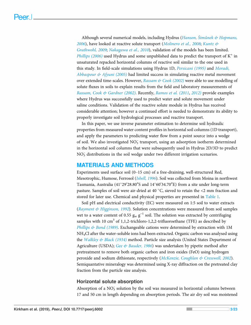
Point-source solute infiltrationPerspex wedges were constructed with the same dimensions described by Li, Zhang & Ren(2003) and packed with dry soil (water content of 0.2 g g-1) to a bulk density of 0.95 g cm-3.All solutions were applied to the 15� corner of the wedge at a depth of five cm(Fig. 1) with a peristaltic pump set to deliver solution at 50 cm3 h-1, equivalent to adripper output of 1,200 cm3 h-1 in a 360� flow environment.

Figure 2 shows the two irrigation scenarios applied to the wedge experiments.Both treatments were irrigated for 0.5 h (equivalent to 25 cm3 of solution) with theNO3

– solution applied to the horizontal columns, that is 110 mmolc NO3– cm-3. This was

immediately followed by a 1.5 h application of solute free water (75 cm3). The soil waseither (i) sampled immediately after the water application (Scenario A) or (ii) allowed torest for 16 h before irrigating again with water for 6 h (300 cm3) prior to sampling(Scenario B). That is, a total of 375 cm3 of water was applied to the wedge in Scenario Bwith samples being taken 24 h after initial application of the solute. A single replicatewas used for Scenario A and Scenario B was duplicated.

Soil was sampled using the method described by Li, Zhang & Ren (2003). Briefly, afive cm grid was placed over the column and a soil core (two cm internal diameter) takenfrom the centre of each grid. Additional soil samples were taken at the edge of the wettingfront. The soil from the core was sub-sampled to determine gravimetric water content

Application point 15O

40 cm

40 cm

Figure 1 Geometry of the wedge apparatus. Full-size DOI: 10.7717/peerj.6002/fig-1

Kirkham et al. (2019), PeerJ, DOI 10.7717/peerj.6002 5/23

and total NO3– concentration (solution and adsorbed). Wet soil was extracted with 2M KCl

(1:10 soil: KCl ratio) and analysed on an Alpkem autoanalyser (Rayment & Higginson,1992). Calculations of total NO3

– partitioned into the solution and the amount of adsorbedNO3

– were done using the adsorption isotherm determined from the horizontalcolumn data (described below).

Nitrate adsorption isothermPartitioning of NO3

– between the adsorbed and solution phases, over the range of soilsolution concentrations in the columns, was measured by displacing the soil solutionwith TFE (Phillips & Bond, 1989). The Langmuir equation (Eq. (1)) was then fitted to thedata to describe the NO3

– adsorption isotherm.

Ca ¼ Cmax fCw

1þ fCw; (1)

where Ca is the concentration of adsorbed solute (mmolc g-1), Cw is the concentration

of solute in the soil solution (mmolc cm-3), Cmax is the maximum amount of solute

that can be adsorbed by the soil (g cm-3), and f determines the magnitude of the initialslope of the isotherm (Sposito, 1989).

StartWater + solute

StartWater + solute

End water/Sample column

Time (hr)

Time (hr)

Endsolute

0 1 2 18 19 20 21 22 23 24

0 1 2 18 19 20 21 22 23 24

Endsolute

Pausewater

Resumewater

Samplecolumn

(A)

(B)

Figure 2 Schematic of the two irrigation scenarios (A) and (B) applied to the wedge columns.Full-size DOI: 10.7717/peerj.6002/fig-2

Kirkham et al. (2019), PeerJ, DOI 10.7717/peerj.6002 6/23

Cmax and f were determined using the Gauss–Newton nonlinear curve model in thestatistical program SAS (version 9.1; SAS, Cary, NC, USA). Cmax and f were determinedto be 23.17 (95% confidence interval (CI) ± 3.43) and 0.00766 (95% CI ± 0.00194),respectively.

Hydrus flow equationsWater flow is described by the Richards equation modified to describe horizontal flowin one dimension with no loss of water due to evaporation of root uptake (Šimůneket al., 2008):

@u

@t¼ @

@xK@c

@x

� �;

where θ is the volumetric water content (cm3 cm-3), t is time (min), x is the horizontaldistance (cm), c is the water tension (cm), and K is the hydraulic conductivity (cm min-1)given by:

Kðc; xÞ ¼ KsatðxÞKrðh; xÞ;where Kr is the relative hydraulic conductivity (no unit) and Ksat is the saturated hydraulicconductivity (cm min-1; Šimůnek et al., 2008).

The modified form of the Richards equation that describes water movement intwo dimensions assuming no loss of water through root uptake or evaporation can bewritten (Šimůnek, Van Genuchten & Šejna, 2006):

@u

@t¼ @

@xiK KA

ij@c

@xj

� �þ KA

iz

� �

where xi (i = 1,2) are the spatial coordinates (cm), and KAij and KA

iz are components of adimensionless anisotropy tensor KA. Assuming flow is isotropic (i.e. K is equal inhorizontal and vertical directions) the diagonal entries of KA

ij equal one and theoff-diagonal entries equal zero (Šimůnek, Van Genuchten & Šejna, 2006).

In the two-dimensional flow scenario K is given by:

Kðc; xÞ ¼ Ksatðx; zÞKrðh; x; zÞ:If the modified form of the Richards equation is applied to planar flow in a vertical crosssection, x1 = x is the horizontal coordinate and x2 = z is the vertical coordinate. This equationcan also describe axisymmetric flow when x1 = x represents a radial coordinate (Gardenaset al., 2005). The transcripts i and j denote either the x or z coordinate.

To solve the Richards equation, Hydrus implements the soil hydraulic functions of thevan Genuchten–Mualem to describe unsaturated hydraulic conductivity in terms of soilwater retention parameters (Šimůnek, Van Genuchten & Šejna, 2006). Water retention isdescribed by Šimůnek, Van Genuchten & Šejna (2006) as:

uðcÞ ¼ urus � ur

½1þ acj jn�m c, 0

us c � 0

8<:

Kirkham et al. (2019), PeerJ, DOI 10.7717/peerj.6002 7/23

and unsaturated conductivity is written (Šimůnek, Van Genuchten & Šejna, 2006):

KðcÞ ¼ KsSle 1� ð1� S1=me Þmh i

2 c, 0

where:

m ¼ 1� 1=n; n > 1

and:

Se ¼ u� urus � ur

In the above equations θr is the residual water content (cm3 cm-3), θs is the saturatedwater content (cm3 cm-3), a (cm-1), n (no unit), and l (no unit) are curve fitting parametersfor the hydraulic conductivity function and Se is the effective water content (cm

3 cm-3).When the van Genuchten–Mualem model is used to solve Richards equation in Hydrus

there are six soil hydraulic parameters required (θr, θs, a, n, l, and Ksat).The Langmuir equation was used to predict the reactive solute transport. In Hydrus,

desorption of a nontransforming solute is described by the generalised nonlinear equation(Šimůnek, Van Genuchten & Šejna, 2006):

Ca ¼ ksCvw

1þ fCvw

; (2)

and:

@Ca

@t¼ ksvCv�1

w

ð1þ fCvwÞ2

@Cw

@tþ Cv

w

1þ fCvw

@ks@t

� ksC2vw

ð1þ fCvwÞ2

@f@t

þ ksCvw lnCw

ð1þ fCvwÞ2

@v

@t; (3)

where ks (cm3 g-1), v (dimensionless), and f (cm3 g-1) are constants. In the case of the

Langmuir equation, ks = Cmax f (where Cmax and f are the Langmuir equation constantsfrom Eq. (1)) and v = 1.

Estimation of flow equations parametersSoil hydraulic parameters for the van Genuchten equation were determined using theinverse optimisation procedure in Hydrus 1D (Šimůnek et al., 2008). Water profile datafrom the soil columns in Set A were used, after removing obvious outliers in the datathat were determined to be due to soil loss during column sampling (Hopmans et al., 2002).The initial water content was set to 0.15 (cm3 cm-3), the measured water content ofthe repacked columns, for all optimisations. Free water absorption was simulated byapplying constant water content boundary condition of 0.64 (cm3 cm-3) to the opening ofthe column. The lower boundary condition was set to free drainage. The maximumnumber of iterations was set to 50 and 86 water content points across five time steps wereused in the inverse scenario from the Set A column experiments. Weighting of inverse datawas by standard deviation and an equal weighting was applied to all the water contentvalues. Residual soil water content (θr), θs, and Ksat were set or optimised depending on theoptimisation scenario (Fit All is the term applied when all parameters were optimisedand Set Measured is used when θr, θs, and Ksat were set to independently measured values).

Kirkham et al. (2019), PeerJ, DOI 10.7717/peerj.6002 8/23

The remaining empirical parameters, a, n, and l were fitted by running the inverseparameter estimation option in Hydrus 1D. The initial values of a, n, and l werebased on the default values given for the Loam soil in Hydrus 1D (a = 1.56, n = 0.173,and l = 0.5).

Initial estimates for θr and θs were 0.05 and 0.58 (cm3 cm-3) and Ksat was set to0.10 cm min-1. Saturated soil water content (θs) and Ksat values were independentlymeasured in falling head Ksat experiments (Reynolds et al., 2002). A column ofwater (4.2 cm in diameter and 12 cm high) was applied to wet repacked soil core packed toa bulk density of 1.0 with air dry soil sieved to <2 mm. The soil cores were two cm high andhad an internal diameter the same as the water column sitting above it. Triplicatemeasurements of conductivity were recorded on four separate cores. Residual soil watercontent (θr) was estimated based on the air-dry soil water content.

The Rosetta PTF model (Schaap, Leij & Van Genuchten, 2001) was used to estimate soilhydraulic properties as a comparison against the inverse modelling method. The soilparticle size measurements (Table 1) and bulk density (1.03 g cm-3) were used to estimatesoil hydraulic parameters. In a second prediction, moisture retention at -33 and-1,500 kPa (0.34 and 0.22 cm3 cm-3, respectively) were also included as inputs intoRosetta. The water content at -33 kPa was determined on a suction table apparatus and-1,500 kPa were determined using pressure plate apparatus (Cresswell, 2002).

Modelling water and solute absorption in soil wedgesHydrus 2D/3D was used to model water distribution in the horizontal column experimentsbased on the same initial and boundary conditions used in Hydrus 1D during inverseoptimisation. Horizontal flow in Hydrus 2D/3D was simulated by setting the geometry to a2D horizontal plane. The geometry of the flow domain was set to a column two cm indiameter and 50 cm long. Soil hydraulic parameters having the lowest values for theobjective function were used to simulate water absorption. Nitrate absorption waspredicted by applying a third-type (Cauchy) solute boundary at the inlet of the column(x = 0 cm) at a constant concentration of 110 mmol NO3

– cm-3. Bulk density was set to themeasured value of 1.03 g cm-3, longitudinal and transverse dispersivities were set to0.3 and 0.03 cm, respectively (Ajdary et al., 2007), and the diffusion coefficient wasneglected as it was considered negligible relative to the dispersion (Hanson, Šimůnek &Hopmans, 2006; Ajdary et al., 2007). Parameters for the Langmuir equation (Eq. (1)) todescribe NO3

– adsorption were determined from the data measured in column Set B.

Modelling water and solute in horizontal columnsTo simulate water and NO3

– distribution in the wedge experiments, a 40 � 40 cm flowdomain was created in a 2D axisymmetrical vertical flow geometry. The infiltration pointat five cm depth was represented by a semicircle with three cm radius. The flux from thesource was 10.61 cm h-1 (Eq. (4)), equivalent to a dripper output of 1,200 cm3 h-1.

s ¼ Q4p r2

; (4)

Kirkham et al. (2019), PeerJ, DOI 10.7717/peerj.6002 9/23

where s is the flux from the surface of the source (cm h-1), Q is the total volumetric flux(cm3 h-1), and r is the radius of the spherical source (cm).

The finite element mesh of the flow domain, which determines the level of modelresolution in the calculations, was set to 0.5 cm in both z and h directions. No flux wasallowed through the column boundaries. The infiltration source was set as a variable fluxboundary so that water and solute applications could be controlled according to thetwo irrigation scenarios described for the wedge columns (Fig. 2). Nitrate absorption waspredicted in the same way as for the horizontal columns. The time-variable boundarycondition was used to apply the solute (110 mmolc NO3

– cm-3) only for the first 0.5 h ofwater application to the column.

Statistical analysisThe root mean square error (RMSE) was calculated as the error between the measured andsimulated water content and NO3

– concentrations. Comparisons of the RMSE valueswith predictions from different parameter sets allowed those that produced the lowesterrors to be identified. Comparisons of simulated RMSE values with those calculated frommeasured data allowed the significance of the model error to be assessed in relationto measurement error. This method has been commonly used to measure the quality ofmodel predictions in previous studies (Skaggs et al., 2004; Ajdary et al., 2007; Arbat et al.,2008; Patel & Rajput, 2008). Part of the inverse modelling in Hydrus 1D allowscalculation of a correlation matrix that specifies the correlation between the fittedcoefficients and statistical information about the fitted parameters.

RESULTSParameter determination and model validation in horizontal columnsValues for soil hydraulic parameters estimated from column Set A are presented in Table 2.The two inverse scenarios produced slightly differing values, with the Fit All parametershaving a lower value for the objective function � than the Set Measured suggestingthat the former gave a slightly closer fit between the predicted and measured soil waterprofiles. The 95% CIs for the optimised values for a, n, and l where smaller compared tothe values when all parameters were optimised. The parameters in the Fit All scenariohad higher uncertainty and greater correlation between fitted parameters compared to theSet Measured parameters (Tables 2 and 3). The correlation matrix shows there werethree high values in the Fit All parameter function compared to one in the Set Measuredresults; a and n being highly correlated (Table 3, bold entries). High correlation values

Table 2 Parameter estimation results for the Fit All and Set Measured parameter sets.

Inversescenario

θr (cm3 cm-3) θs (cm3 cm-3) α (cm-1) n Ksat (LT-1) l F

Fit All 0.112 (0.247) 0.560 (0.007) 0.036 (0.006) 2.030 (0.684) 0.115 (0.061) 3.847 (5.442) 0.014

Set Measured 0.054 (0.003*) 0.580 (0.04*) 0.038 (0.005) 2.335 (0.279) 0.104 (0.029*) 3.175 (0.578) 0.020

Notes:Values in parentheses show the 95% confidence intervals of the estimated parameters. � indicates the value of the objective function.* Independently measured.

Kirkham et al. (2019), PeerJ, DOI 10.7717/peerj.6002 10/23

(magnitude >0.9) indicate parameter nonuniqueness and a correspondingly highuncertainty (Hopmans et al., 2002; Šimůnek & Van Genuchten, 1996). The optimised valueof θr was 0.112 and the 95% CI that ranged from -0.135 to 0.359, which includesthe measured value (0.054 ± 0.003). Saturated water content (θs) was 0.56 (0.553–0.567)and was significantly different from the independently measured values (0.58 ± 0.04;Table 2). The measured Ksat (0.104 ± 0.0299) fall within the 95% CI [0.054–0.176;mean best fit value of 0.115] of the optimised value.

The two parameter sets were tested against independently measured data from thehorizontal columns (Column data Set B) and the point-source wedge experiments.Predicted water distributions and measured water content in the horizontal columns fromcolumn Set B are shown in Fig. 3A. We have plotted θ and NO3

– profiles against theBoltzmann variable X (distance/√time; cm s-1/2; Smiles et al., 1978; Phillips & Bond, 1989).Both parameter sets showed similarly good correspondence to the measured data(continuous and dotted lines), which is confirmed by the RMSE and R2 values (Table 4).Accurate predictions of θ profiles after absorbing water for 80 and 320 min are notsurprising given that data from Set A (27–70 min) are not statistically different from Set Bwhen normalised against the Boltzmann variable. The results, however, do show thatunder the unsaturated absorption scenario, predictions made for longer times (80 and320 min) are still accurate when the predictions are extended beyond the range ofoptimised data. The consistency between predictions based on short time θ and NO3

– data(Set A) and longer time θ and NO3

– data (Set B) further demonstrate the experimentshad a good degree of repeatability and produced consistent data across a range oftime scales.

In comparison, predicted water content using soil hydraulic parameters determined byRosetta are shown in Fig. 4. These data show the piston front to be significantly behindthe measured data (combined data from column Set A and B) especially when thewater content at -33 and -1,500 kPa are included in the model. Removal of the FeO beforedetermining the sand, silt, and clay content did not improve the predictions of waterretention parameters or saturated hydraulic conductivity. Deriving the water retention

Table 3 Correlation matrix of the inverse function.

Fit All θr θs α n Ksat l

θr 1.000

θs 0.016 1.000

a 0.977 -0.046 1.000

n 0.656 –0.243 0.561 1.000

Ksat -0.753 0.118 -0.649 -0.976 1.000

l -0.975 -0.149 -0.941 -0.605 0.737 1.000

Set Measured α n l

a 1.000

n 0.937 1.000

l -0.283 0.063 1.000

Kirkham et al. (2019), PeerJ, DOI 10.7717/peerj.6002 11/23

parameters and saturated hydraulic conductivity with Rosetta, values that use PTFs topredict the Van Genuchten parameters, produced significant inaccuracies in thepredictions (see Fig. 4). In these experiments they are certainly less accurate thanparameters derive from inverse modelling (Fig. 3).

The predicted NO3– distribution is shown in Fig. 3B. The measured and predicted

NO3– distributions were compared from both Set A (27–70 min) and Set B

A

vmc(

3mc

3-)

0.0

0.2

0.4

0.6

B

X (cm s-1/2)

0.0 0.1 0.2 0.3 0.4 0.5

ON

noituloslioS3-

(mclo

m3-)

0

20

40

60

80

100

120

140

μq

Figure 3 (A) Fits of the Fit All (solid line) and Set Measured (dotted line) parameters to the measuredwater profile data (squares) from column Set B not included in the inverse optimisation. (B) Fits forsoil solution NO3

–. Full-size DOI: 10.7717/peerj.6002/fig-3

Table 4 Root mean square error (RMSE) of water and NO3– profiles determined using the Fit All and

Set Measured parameters in comparison to the measured data in the horizontal column experimentspresented in Fig. 3.

Inverse scenario θv (cm3 cm-3) NO3– (μmolc cm

-3 soln)

RMSE R2 RMSE R2

Fit All 0.04 0.89 7.50 0.97

Set Measured 0.05 0.91 7.96 0.97

Measured† 0.04 6.19

Note:† “Measured” indicates the variation in the measured data calculated from the second set of horizontal soil columnswhere two NO3

– and water measurements were made at identical points and times.

Kirkham et al. (2019), PeerJ, DOI 10.7717/peerj.6002 12/23

(80 and 320 min) because the NO3– distribution was not used in the inverse optimisation.

The good prediction of NO3– distribution by the two parameter sets, when the Langmuir

isotherm parameters were included in the simulations, is confirmed by the R2 and RMSEvalues (Table 4). Due to the inaccuracy of water content prediction using Rosetta, no NO3

–

data are presented.

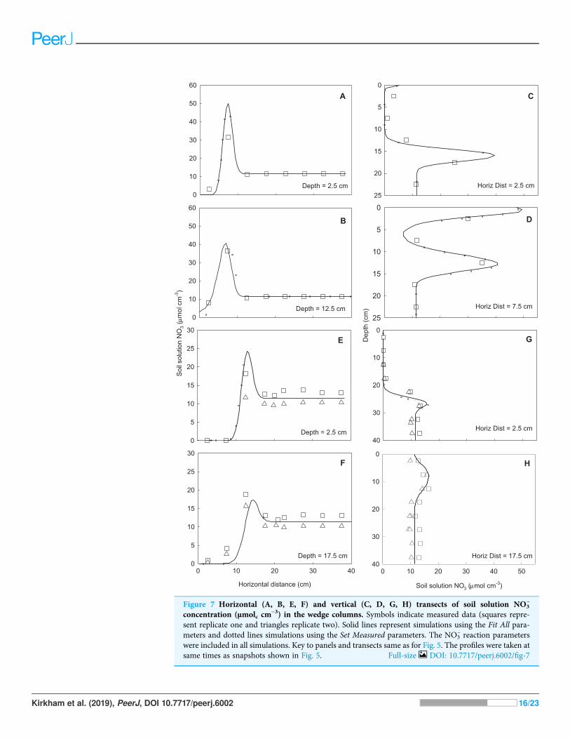
Model validation using 3D wedge infiltrationThe predicted distributions of water and NO3

– throughout the soil wedge after thetwo irrigation scenarios are shown in Fig. 5. This figure also shows the positionsof horizontal and vertical transects presented in Figs. 6 and 7. These figures show theagreement between the measured and predicted water and NO3

– profiles in the wedge.Comparisons of the RMSE and R2 calculations indicated that both the Fit All andSet Measured parameter sets predicted very similar distributions, although the Fit Allparameters produced slightly better predictions of NO3

– distribution in the longerirrigation scenario. The measured RMSE, calculated from columns where duplicatemeasurements were taken at identical times and locations, were similar to the RMSE of thepredicted values (Table 5). This indicates that the errors between the measured andpredicted values were very similar to the errors of replicate measurements at identicalpoints and times in the wedge experiments. The predictions achieved using thetwo parameter sets were therefore considered to be suitable to estimate water andNO3

– distribution in the point-source flow scenario of the wedge column. The “SetMeasured” parameters are preferred because there is less auto correlation between thefitted parameters (a, n, l).

X (cm sec-1/2)

0.0 0.1 0.2 0.3 0.4 0.5

vmc(

3mc/

3 )

0.1

0.2

0.3

0.4

0.5

0.6

0.7

θ

Figure 4 Predicted volumetric water content using Rosetta derived soil hydraulic parameters andmeasured water profile data (squares) against the Boltzmann variable (X). The solid line representsderived parameters using particle size data measured after removal of iron oxides and no water contentdata; the dash line represents parameters predicted using particle size without removing iron oxides andwithout water content data; the dash-dot–dash line refers to parameter predicted using particle sizewithout removing iron oxides and with soil water content at -33 and -1,500 kPa; the dash-dot-dot–dashline refers to parameters predicted using particle size after removing iron oxides and with soil watercontent at -33 and -1,500 kPa. Full-size DOI: 10.7717/peerj.6002/fig-4

Kirkham et al. (2019), PeerJ, DOI 10.7717/peerj.6002 13/23

DISCUSSIONInverse optimisation using Hydrus-1D can be used to effectively estimate soil hydraulicproperties from simple 1D flow experiments. The flow parameters derived from1D columns were suitable for describing flow under more complex 3D flow scenarios.These results show that the use of absorption columns offers an alternative to PTFmethods and has the advantage that the parameters are determined using data from theactual soil type under consideration.

Comparisons of optimised parameters with independently measured data in thehorizontal column showed that the fitted parameters were able to accurately predict waterdistribution in these flow scenarios. Further, water distribution could be accurately

Figure 5 Estimation of water and NO3– in the wedge experiment scenario using the Set Measured

parameters. (A) and (C) show water content (cm3 cm-3) and NO3– (mmol cm-3), respectively, for

irrigation scenario A (2 h experiment, Fig. 2). (B) and (D) show water content (cm3 cm-3) andNO3

– (mmol cm-3), respectively, for irrigation scenario B (24 h experiment, Fig. 2). Horizontal andvertical transects and their symbols correspond to the water and solute profile plots in Figs. 6 and 7.

Full-size DOI: 10.7717/peerj.6002/fig-5

Kirkham et al. (2019), PeerJ, DOI 10.7717/peerj.6002 14/23

Depth = 12.5 cm0.0

0.1

0.2

0.3

0.4

0.5

0.6

Depth = 2.5 cmv

mc(3

mc3-)

0.0

0.1

0.2

0.3

0.4

0.5

0.6Horiz Dist = 2.5 cm

0

5

10

15

20

25

Horiz Dist = 7.5 cm

)mc(

htpeD

0

5

10

15

20

25

Depth = 2.5 cm0.0

0.2

0.4

0.6

Depth = 17.5 cm

Horizontal distance (cm)

0 5 10 15 20 25 300.0

0.2

0.4

0.6

Horiz Dist = 2.5 cm0

10

20

30

40

Horiz Dist = 17.5 cm

v (cm3 cm-3)

0.0 0.2 0.4 0.6

0

10

20

30

40

A

B

C

D

E

F

G

H

θ

θ

Figure 6 Horizontal (A, B, E, F) and vertical transects (C, D, G, H) of water content (cm3 cm-3) in thewedge columns. The symbols indicate measured data (squares represent replicate one and trianglesreplicate two). Solid lines represent simulations using the Fit All parameters and the dotted linessimulations using the Set Measured parameters. A to D show transects from irrigation scenario A(2 h experiment, Fig. 2) and E to H show transects from irrigation scenario B (24 h experiment, Fig. 2).Location of transects is shown in Fig. 5. The profiles were taken at same times as snapshots shown inFig. 5. Full-size DOI: 10.7717/peerj.6002/fig-6

Kirkham et al. (2019), PeerJ, DOI 10.7717/peerj.6002 15/23

Depth = 12.5 cm0

10

20

30

40

50

60

Depth = 2.5 cmO

NnoituloslioS

3(

mclom

3-)

0

10

20

30

40

50

60

Horiz Dist = 2.5 cm

0

5

10

15

20

25

Horiz Dist = 7.5 cm)mc(

htpeD

0

5

10

15

20

25

Horiz Dist = 2.5 cm

0

10

20

30

40

Horiz Dist = 17.5 cm

Soil solution NO3 ( mol cm-3)

0 10 20 30 40 50

0

10

20

30

40

Depth = 2.5 cm0

5

10

15

20

25

30

Depth = 17.5 cm

Horizontal distance (cm)

0 10 20 30 400

5

10

15

20

25

30

A

B

C

D

E

F

G

H

μ

μ

Figure 7 Horizontal (A, B, E, F) and vertical (C, D, G, H) transects of soil solution NO3–

concentration (μmolc cm-3) in the wedge columns. Symbols indicate measured data (squares repre-

sent replicate one and triangles replicate two). Solid lines represent simulations using the Fit All para-meters and dotted lines simulations using the Set Measured parameters. The NO3

– reaction parameterswere included in all simulations. Key to panels and transects same as for Fig. 5. The profiles were taken atsame times as snapshots shown in Fig. 5. Full-size DOI: 10.7717/peerj.6002/fig-7

Kirkham et al. (2019), PeerJ, DOI 10.7717/peerj.6002 16/23

predicted for absorption periods four times longer than the data used in the inverseoptimisation. This provides preliminary evidence that the parameters can predict waterdistribution outside the range of fitted values. However, this result is not surprising becausethe measured water content profiles coalesce to a single curve when presented against theBoltzmann variable X (cm s-1/2). Further evidence for this was provided by testing theparameters in the alternative point-source 3D flow scenario. The results presentedin this paper demonstrate there is scope to use soil hydraulic parameters obtained fromsimple horizontal absorption experiments to accurately estimate water flow under morecomplex 3D conditions in uniform repack soil conditions (isotropic).

The inverse optimisations in this study produced two parameter sets that were capableof providing good predictions of water flow in the two flow scenarios. Hopmans et al.,(2002) suggests that if various parameter sets produce similar model outcomes, the soilhydraulic parameters may be unidentifiable and the inverse optimisation may be ill-posed.However, our data (Table 2) shows that the values identified in the two scenarios arewithin the 95% CI estimates of the predictions; the difference between the parameter setsare therefore not significant. Limiting the number of parameters optimised in theinverse procedure reduced the uncertainty of the fitted parameters without significantlyaffecting the accuracy of model predictions. Further, the Fit All scenario gave highcorrelations of three parameters in comparison to the one high value for the Set Measuredscenario (Table 3). Limiting the number of parameters in the inverse scenario wasshown to be advantageous because parameter variation was reduced. These findings areconsistent with the recommendations of Hopmans et al. (2002) but contrast with thestudy of Sonnleitner, Abbaspour & Schulin (2003). The latter work indicated thatmaximising the number of variables in the inverse optimisation increased the ability ofparameters to describe water flow in alternative scenarios.

In our wedge study, only minor differences were observed between predictions when thenumber of optimised parameters was reduced. Furthermore, reducing the number ofparameters in the inverse optimisation was advantageous because parameter uncertaintywas reduced (Table 2). Our results show that, where practical, there is benefit inconducting additional measurements to estimate θs and Ksat, which are two of the mostsensitive parameters of the model (Arbat et al., 2008). The benefits of using measured

Table 5 Root mean square error (RMSE) of the fit of the two parameter sets used to predict waterand NO3

– distribution in the wedge experiments.

Parameters Irrigation treatment θv (cm3 cm-3) NO3– (μmolc cm

-3 solution)

RMSE R2 RMSE R2

Fit All Scenario A 0.04 0.94 2.40 0.95

Scenario B 0.03 0.97 3.05 0.81

Set Measured Scenario A 0.04 0.96 2.16 0.95

Scenario B 0.02 0.98 3.43 0.76

Measured† 0.03 2.64

Note:† “Measured” RMSE values indicate the variation in the measured data calculated from the wedge experiments fromIrrigation Scenario B columns where two NO3

– and water measurements were made at identical points in the wedges.

Kirkham et al. (2019), PeerJ, DOI 10.7717/peerj.6002 17/23

parameters, in combination with inverse modelling of water content data, has also beendemonstrated by Kandelous et al. (2011). In these columns, hydraulic conductivity is notindependently measured; rather sorptivity is measured and the hydraulic conductivitymust be inferred with a model.

Including solute reaction parameters enables the Hydrus model to accurately predictreactive solute distribution in the soil. The retardation in the NO3

– relative to the inflowingwater indicates that the solute was adsorbed by the soil. Sorption of NO3

– wasincluded in Hydrus by using the Langmuir equation to approximate the partitioning ofNO3

– between the soil solution and the adsorbed phases. The Langmuir equation has beenused previously to describe solute adsorption in soil (Katou, Clothier & Green, 1996;Qafoku, Sumner & Radcliffe, 2000; Phillips, 2006).

The distribution of solutes adsorbed to soil during water flow has been simulated underpoint-source infiltration in previous studies using Hydrus 2D/3D (Hanson, Šimůnek &Hopmans, 2006). However, validation under these flow scenarios has received littleattention. Ben-Gal & Dudley (2003) observed that predictions of reactive P transport froma drip irrigation system showed a similar distribution to measured data, but they did notmake any statistical comparisons. Reactive solute transport was previously validatedunder other flow scenarios (Persicani, 1995; Moradi, Abbaspour & Afyuni, 2005).Our results validate the inclusion of the Langmuir equation in Hydrus for the prediction ofreactive solute movement for 1D and 3D flow conditions. Furthermore, the resultsshow that reactive solute parameters determined from relatively simple 1D adsorptioncolumns can be used to accurately predict solute distribution under 3D conditions.

Other studies that have used Hydrus to predict water movement through soils haveutilised PTFs to estimate soil hydraulic parameters (Epino et al., 1996; Skaggs et al., 2004;Li, Zhang & Rao, 2005; Phillips, 2006; Siyal & Skaggs, 2009). The suitability of parameterspredicted by PTFs relies on the amount of data collected from soils with similarparticle size distribution, bulk density, and water-holding capacity. We investigated use ofthe Rosetta model (Schaap, Leij & Van Genuchten, 2001) to obtain parameters for thesame Red Ferrosol used here, but it provided less accurate estimates of water distributionin comparison to parameters determined from inverse modelling (Fig. 4). The high valueof the pore connectivity parameter, l (Table 2), that resulted from inverse optimisationis in contrast to the value of 0.5 used on the Rosetta model (Cook & Cresswell, 2007).This difference may explain the limitations of Rosetta to accurately predict water flow inthe repacked columns in these particular experiments.

This finding contrasts with those of Kandelous & Šimůnek (2010a) where parametersestimated from Rosetta produced acceptable predictions of water movement in laboratorystudies. The differing results in our study may be in part due to the limited data forAustralian Red Ferrosols available in the Rosetta soil database. In general, thispaper confirms that inverse optimisation is advantageous provided enough data hasbeen collected over a sufficient range of water contents (Šimůnek et al., 2000; Sonnleitner,Abbaspour & Schulin, 2003). The use of inverse optimisation applied to horizontalinfiltration columns provides a simple technique to accurately determine reactionparameters.

Kirkham et al. (2019), PeerJ, DOI 10.7717/peerj.6002 18/23

If parameters determined from inverse optimisation are to successfully describe waterflow in alternative scenarios the soil properties must be the same. This was achieved in ourlaboratory because careful packing was possible in both the horizontal columns and soilwedges. For a field scenario, a similar method of predicting water and solute flow would needlaboratory experiments on undisturbed cores. Similarly, Kandelous & Šimůnek (2010a)found that parameters suitable for describing water movement in packed laboratory columnswere not capable of describing water distribution in an undisturbed field soil.

CONCLUSIONInverse modelling procedures in Hydrus confirm that soil hydraulic parameterscan be reliably obtained from simple 1D diffusive water uptake soil column studies.The derived parameters are capable of accurately describing diffusive water movementover extended times and in alternative dynamic flow scenarios to those in which they werefitted. These results demonstrate that simple water uptake column experiments can beused to provide suitable flow conditions for accurate determination of reaction parametersunder dynamic flow conditions. Reducing the number of parameters in the optimisationprocedures by imposing independently measured values for θs, θr, and Ksat decreasedparameter uncertainty (or increased parameter uniqueness) without significantlyimpacting the accuracy of model predictions. These results show there is merit in pursuingthis method in more complex scenarios since it may provide a simpler and cheaper way ofdetermining hydraulic parameters in field conditions.

Solution NO3– and adsorbed NO3

– concentrations collected from a combined wateruptake-NO3

– tracer test provided the data to fit the reaction parameters for the Langmuirisotherm, which in turn were included in the Hydrus model to predict reactivesolute transport. We have demonstrated the ability of HYDRUS to integrate unsaturatedflow processes and independently determined reactive transport processes based onindependent experiments involving the complex interplay of dynamic flow andreactive transport.

ACKNOWLEDGEMENTSWe thank Dr Freeman Cook for his assistance with Hydrus modelling and Dr David Smilesfor providing his expertise in experimental design and analysis.

ADDITIONAL INFORMATION AND DECLARATIONS

FundingAn Australian Federal Government Postgraduate Scholarship supported Dr. Kirkam’sresearch. The funders had no role in study design, data collection and analysis, decision topublish, or preparation of the manuscript.

Grant DisclosureThe following grant information was disclosed by the authors:Australian Federal Government Postgraduate Scholarship.

Kirkham et al. (2019), PeerJ, DOI 10.7717/peerj.6002 19/23

Competing InterestsThe authors declare that they have no competing interests.

Author Contributions� James M. Kirkham conceived and designed the experiments, performed the experiments,analyzed the data, contributed reagents/materials/analysis tools, prepared figures and/ortables, authored or reviewed drafts of the paper, approved the final draft.

� Christopher J. Smith conceived and designed the experiments, analyzed the data,contributed reagents/materials/analysis tools, authored or reviewed drafts of the paper,approved the final draft.

� Richard B. Doyle conceived and designed the experiments, authored or reviewed draftsof the paper, approved the final draft.

� Philip H. Brown conceived and designed the experiments, authored or reviewed drafts ofthe paper, approved the final draft.

Data AvailabilityThe following information was supplied regarding data availability:

Raw data is available as Supplemental Files.

Supplemental InformationSupplemental information for this article can be found online at http://dx.doi.org/10.7717/peerj.6002#supplemental-information.

REFERENCESAjdary K, Singh DK, Manoj Singh AK, Khanna M. 2007. Modelling of nitrogen leaching from

experimental onion field under drip fertigation. Agricultural Water Management 89(1–2):15–28DOI 10.1016/j.agwat.2006.12.014.

Alpkem. 1992. The flow solution. Wilsonville: Alpkem Corporation.

Arbat G, Puig-Bargues J, Bonany J, Barragan J, Ramirez De Cartagena F. 2008.Monitoring soilwater status for micro-irrigation management versus modelling approach.Biosystems Engineering 100(2):286–296 DOI 10.1016/j.biosystemseng.2008.02.008.

Ben-Gal A, Dudley LM. 2003. Phosphorus availability under continuous point source irrigation.Soil Science Society of America Journal 67(5):1449–1456 DOI 10.2136/sssaj2003.1449.

Cook FJ, Cresswell HP. 2007. Estimation of soil hydraulic properties. In: Carter MR,Gregorich EG, eds. Soil samplIng and methods of analysis, canadian society of soil science.Boca Raton: Taylor and Francis, LLC, 1139–1161.

Cook FJ, Thorburn PJ, Fitch P, Bristow KL. 2003. WetUp: a software tool to displayapproximate wetting patterns from drippers. Irrigation Science 22(3–4):129–134DOI 10.1007/s00271-003-0078-2.

Cote CM, Bristow P, Charlesworth PB, Cook FJ, Thorburn PJ. 2003. Analysis of soil wettingand solute transport in subsurface trickle irrigation. Irrigation Science 22(3–4):143–156DOI 10.1007/s00271-003-0080-8.

Cresswell HP. 2002. The soil water characteristic. In: McKenzie N, Coughlan K, Cresswell HP, eds.soil physical measurement and interpretation for land evaluation. Collingwood: CSIROPublishing, 59–84.

Kirkham et al. (2019), PeerJ, DOI 10.7717/peerj.6002 20/23

Epino A, Mallants D, Vanclooster M, Feyen J. 1996. Cautionary notes on the use of pedotransferfunctions for estimating soil hydraulic properties. Agricultural Water Management29(3):235–253 DOI 10.1016/0378-3774(95)01210-9.

Gardenas AI, Hopmans JW, Hanson BR, Šimůnek J. 2005. Two-dimensional modeling of nitrateleaching for various fertigation scenarios under micro-irrigation. Agricultural WaterManagement 74(3):219–242 DOI 10.1016/j.agwat.2004.11.011.

Gee GW, Bauder JW. 1986. Particle-size analysis. In: Klute A, ed. Methods of soil analysis. Part 1.Physical and mineralogical methods. Madison: ASA and SSSA, 383–411.

Hanson BR, Šimůnek J, Hopmans JW. 2006. Evaluation of urea–ammonium–nitrate fertigationwith drip irrigation using numerical modeling. Agricultural Water Management86(1–2):102–113 DOI 10.1016/j.agwat.2006.06.013.

Hopmans JW, Šimůnek J , Romano N, Durner W. 2002. Inverse methods. In: Dane JH, Topp GC,eds.Methods of soil analysis. Part 4. Physical methods Chapter. Vol. 3. Madison: SSSA, 963–1008.

Isbell RF. 1996. The Australian soil classification. Collingwood: CSIRO Publishing.

Kandelous MM, Šimůnek J. 2010a. Comparison of numerical, analytical and empirical modelsto estimate wetting pattern for surface and subsurface drip irrigation. Irrigation Science28(5):435–444 DOI 10.1007/s00271-009-0205-9.

Kandelous MM, Šimůnek J. 2010b. Numerical simulations of water movement in asubsurface drip irrigation system under field and laboratory conditions usingHYDRUS-2D. Agricultural Water Management 97(7):1070–1076DOI 10.1016/j.agwat.2010.02.012.

Kandelous MM, Šimůnek J, Van Genuchten MT, Malek K. 2011. Soil water content distributionsbetween two emitters of a subsurface drip irrigation system. Soil Science Society of AmericaJournal 75(2):488–497 DOI 10.2136/sssaj2010.0181.

Katou H, Clothier BE, Green SR. 1996. Anion transport involving competitive adsorption duringtransient water flow in an Andisol. Soil Science Society of America Journal 60(5):1368–1375DOI 10.2136/sssaj1996.03615995006000050011x.

Kuntz D, Grathwohl P. 2009. Comparison of steady-state and transient flow conditions onreactive transport of contaminants in the vadose soil zone. Journal of Hydrology369(3–4):225–233 DOI 10.1016/j.jhydrol.2009.02.006.

Li J, Zhang J, Rao M. 2005. Modeling of water flow and nitrate transport under surface dripfertigation. Transactions of the ASAE 48(2):627–637 DOI 10.13031/2013.18336.

Li J, Zhang J, Ren J. 2003. Water and nitrogen distribution as affected by fertigation ofammonium nitrate from a point source. Irrigation Science 22(1):19–30.

Mallants D, Antonov D, Karastanev D, Perko J. 2007. Innovative in-situ determination ofunsaturated hydraulic properties in deep Loess sediments in North-West Bulgaria. In:Proceedings of the 11th International Conference on Environmental Remediation and RadioactiveWaste Management (ICEM07–7202), Bruges, 1–7.

McKenzie N, Coughlan K, Cresswell H. 2002. Soil physical measurement and interpretation forland evaluation. Melbourne: CSIRO.

Molinero J, Raposo JR, Galindez JM, Arcos D, Guimera J. 2008. Coupled hydrogeologicaland reactive transport modelling of the Simpevarp area (Sweden). Applied Geochemistry23(7):1957–1981 DOI 10.1016/j.apgeochem.2008.02.020.

Moradi A, Abbaspour KC, Afyuni M. 2005. Modelling field-scale cadmium transport below theroot zone of a sewage sludge amended soil in an arid region in Central Iran. Journal ofContaminant Hydrology 79(3–4):187–206 DOI 10.1016/j.jconhyd.2005.07.005.

Kirkham et al. (2019), PeerJ, DOI 10.7717/peerj.6002 21/23

Nakagawa K, Hosokawa T, Wada SI, Momii K, Jinno K, Berndtsson R. 2010.Modelling reactivesolute transport from groundwater to soil surface under evaporation. Hydrological Processes24(5):608–617 DOI 10.1002/hyp.7555.

Patel N, Rajput TBS. 2008. Dynamics and modeling of soil water under subsurface drip irrigatedonion. Agricultural Water Management 95(12):1335–1349 DOI 10.1016/j.agwat.2008.06.002.

Persicani D. 1995. Analysis of leaching behaviour of sludge-applied metals in two field soils.Water, Air, & Soil Pollution 83(1–2):1–20 DOI 10.1007/BF00482590.

Phillips IR. 2006. Modelling water and chemical transport in large undisturbed soil coresusing HYDRUS-2D. Australian Journal of Soil Research 44(1):27–34 DOI 10.1071/SR05109.

Phillips IR, Bond WJ. 1989. Extraction procedure for determining solution andexchangeable ions on the same soil sample. Soil Science Society of America Journal53(4):1294–1297 DOI 10.2136/sssaj1989.03615995005300040050x.

Qafoku NP, Sumner ME, Radcliffe DE. 2000. Anion transport in columns of variable chargesubsoils: nitrate and chloride. Journal of Environmental Quality 29(2):484–493DOI 10.2134/jeq2000.00472425002900020017x.

Rassam DW, Cook FJ. 2002. Numerical simulations of water flow and solute transport applied toacid sulphate soils. Journal of Irrigation and Drainage Engineering 128(2):107–115DOI 10.1061/(ASCE)0733-9437(2002)128:2(107).

Rassam DW, Cook FJ, Gardner EA. 2002. Field and laboratory studies of acid sulphate soils.Journal of Irrigation and Drainage Engineering 128(2):100–106DOI 10.1061/(ASCE)0733-9437(2002)128:2(100).

Rayment GE, Higginson FR. 1992. Australian laboratory handbook of soil and waterchemical methods. Melbourne: Inkata Press.

Reynolds WD, Elrick DE, Youngs EG, Amoozegar A, Booltink HWG, Bouma J. 2002. Saturatedand field-saturated water flow parameters. In: Dane JH, Topp GC, eds. Methods of soil analysis.Part 4. Physical methods. Madison: SSSA, 797–878.

Ramos TB, Simunek J, Goncalves MC, Martins JC, Prazeres A, Castanheira NL, Pereira LS.2011. Field evaluation of a multicomponent solute transport model in soils irrigated with salinewaters. Journal of Hydrology 407(1–4):129–144 DOI 10.1016/j.jhydrol.2011.07.016.

Ramos TB, Simunek J, Goncalves MC, Martins JC, Prazeres A, Pereira LS. 2012.Two-dimensional modeling of water and nitrogen fate from sweet sorghum irrigated with freshand blended saline waters. Journal of Hydrology 111:87–104 DOI 10.1016/j.agwat.2012.05.007.

Schaap MG, Leij FJ, Van Genuchten MT. 2001. Rosetta: a computer program for estimatingsoil hydraulic parameters with hierarchical pedotransfer functions. Journal of Hydrology251(3–4):163–176 DOI 10.1016/S0022-1694(01)00466-8.

Šimůnek J, Hopmans JW, Nielsen DR, Van Genuchten MT. 2000. Horizontal infiltrationrevisited using parameter estimation. Soil Science 165(9):708–717DOI 10.1097/00010694-200009000-00004.

Šimůnek J, Šejna M, Saito H, Sakai M, Van Genuchten MT. 2008. The HYDRUS-1D softwarepackage for simulating the movement of water, heat, and multiple solutes in variably saturatedmedia, Version 4.0, HYDRUS Software Series 3. Riverside: Department of EnvironmentalSciences, University of California Riverside, 315. Available at https://www.pc-progress.com/Downloads/Pgm_hydrus1D/HYDRUS1D-4.08.pdf.

Šimůnek J, Van Genuchten MT. 1996. Estimating unsaturated soil hydraulic properties fromtension disc infiltrometer data by numerical inversion.Water Resources Research 32:2683–2696.

Šimůnek J, Van Genuchten MT, Šejna M. 2006. The HYDRUS software package for simulatingtwo- and three-dimensional movement of water, heat, andmultiple solutes in variably-saturatedmedia.

Kirkham et al. (2019), PeerJ, DOI 10.7717/peerj.6002 22/23

Technical manual. Version 1.0. Prague: PC Progress, 241. Available at https://www.pc-progress.com/downloads/Pgm_Hydrus3D/HYDRUS3D%20Technical%20Manual.pdf.

Siyal AA, Skaggs TH. 2009. Measured and simulated soil wetting patterns under porous claypipe sub-surface irrigation. Agricultural Water Management 96(6):893–904DOI 10.1016/j.agwat.2008.11.013.

Skaggs TH, Trout TJ, Šimůnek J, Shouse PJ. 2004. Comparison of HYDRUS-2D simulations ofdrip irrigation with experimental observations. Journal of Irrigation and Drainage Engineering130(4):304–310 DOI 10.1061/(ASCE)0733-9437(2004)130:4(304).

Smiles DE, Philip JR, Knight JH, Elrick DE. 1978. Hydrodynamic dispersion duringabsorption of water by soil. Soil Science Society of America Journal 42(2):229–234DOI 10.2136/sssaj1978.03615995004200020002x.

Sonnleitner MA, Abbaspour KC, Schulin R. 2003. Hydraulic and transport properties of theplant-soil system estimated by inverse modelling. European Journal of Soil Science54(1):127–138 DOI 10.1046/j.1365-2389.2002.00491.x.

Sposito G. 1989. The chemistry of soils. New York: Oxford University Press.

Van Dam JC, Stricker JNM, Droogers P. 1994. Inverse method to determine soil hydraulicfunctions from multistep outflow experiments. Soil Science Society of America Journal58(3):647–652 DOI 10.2136/sssaj1994.03615995005800030002x.

Vrugt JA, Bouten W. 2002. Validity of first order approximations to describe parameteruncertainty in soil hydrological models. Soil Science Society of America Journal 66(6):1740–1751DOI 10.2136/sssaj2002.1740.

Wagenet RJ, Hutson JL. 1989. LEACHM: Leaching estimation and solute movement – a processedbased model of water and solute movement, transformations, plant uptake and chemical reactionsin the unsaturated zone. Continuum Vol. 2. Ithica: Water Resources Institute, CornellUniversity.

Walkley A, Black IA. 1934. An examination of the Degtjareff method for determining soil organicmatter and a proposed modification of the chromic acid titration method. Soil Science37(1):29–38 DOI 10.1097/00010694-193401000-00003.

Wöhling T, Vrugt JA, Barkle GF. 2008. Comparison of three multiobjective optimizationalgorithms for inverse modeling of vadose zone hydraulic properties. Soil Science Society ofAmerica Journal 72(2):305–319 DOI 10.2136/sssaj2007.0176.

Wu G, Chieng ST. 1995a. Modeling multicomponent reactive chemical transport innonisothermal unsaturated/saturated soils. Part 1. Mathematical model development.Transactions of the ASAE 38(3):817–826 DOI 10.13031/2013.27896.

Wu G, Chieng ST. 1995b. Modeling multicomponent reactive chemical transport innonisothermal unsaturated/saturated soils. Part 2. Numerical simulations. Transactions of theASAE 38(3):827–838 DOI 10.13031/2013.27897.

Kirkham et al. (2019), PeerJ, DOI 10.7717/peerj.6002 23/23