INVERSE UNCERTAINTY QUANTIFICATION OF TRACE PHYSICAL MODEL

PARAMETERS USING BAYESIAN ANALYSIS

BY

GUOJUN HU

THESIS

Submitted in partial fulfillment of the requirements

for the degree of Master of Science in Nuclear, Plasma, and Radiological Engineering

in the Graduate College of the

University of Illinois at Urbana-Champaign, 2015

Urbana, Illinois

Master’s Committee:

Assistant Professor Tomasz Kozlowski, Adviser

Assistant Professor Caleb Brooks

ii

ABSTRACT

Forward quantification of uncertainties in code responses require knowledge of input model

parameter uncertainties. Nuclear thermal-hydraulics codes such as RELAP5 and TRACE do not

provide any information on physical model parameter uncertainties. A framework was developed

to quantify input model parameter uncertainties based on Maximum Likelihood Estimation

(MLE), Bayesian Maximum A Priori (MAP), and Markov Chain Monte Carlo (MCMC)

algorithm for physical models using relevant experimental data.

The objective of the present work is to perform the sensitivity analysis of the code input

(physical model) parameters in TRACE and calculate their uncertainties using an MLE, MAP

and MCMC algorithm, with a particular focus on the subcooled boiling model. The OECD/NEA

BWR full-size fine-mesh bundle test (BFBT) data will be used to quantify selected physical

model uncertainty of the TRACE code. The BFBT is based on a multi-rod assembly with

measured data available for single or two-phase pressure drop, axial and radial void fraction

distributions, and critical power for a wide range of system conditions. In this thesis, the

steady-state cross-sectional averaged void fraction distribution from BFBT experiments is used

as the input for inverse uncertainty algorithm, and the selected physical model’s Probability

Distribution Function (PDF) is the desired output quantity.

iii

ACKNOWLEDGMENTS

First, I want to thank Prof. Tomasz Kozlowski and Prof. Caleb Brooks for making this thesis

possible. In the spring of 2014, Prof. Kozlowski took me into his group and started to guide me

into a research world. Since then, Prof. Kozlowski has been a wonderful mentor to me, both in

respect to research projects and this mater thesis. Prof. Caleb Brooks was the instructor of one

important course about the two-phase flow model. This course helped me a lot in understanding

the two-phase flow and was one important basis of this thesis. Prof. Caleb Brooks is also one of

the committee of this thesis and provides a lot of important comments and suggestion.

I also want to thank Dr. Rijan Shrestha, Xu Wu, Travis Mui and Stefan Tosic. Dr. Shrestha

firstly introduced the inverse uncertainty quantification algorithm in our group and his PhD work

is one very important reference in this thesis. Xu is a PhD candidate in our group and helped me

a lot in both our daily discussions and other research problems. Travis is a graduate student in

our group and he offered great help in the final formatting of the thesis. Stefan is an

undergraduate student in our group and helped in the review this thesis.

I would also want to thank U.S Nuclear Regulatory Commission for funding this work.

iv

TABLE OF CONTENTS

LIST OF FIGURES ....................................................................................................................... vi

LIST OF TABLES ........................................................................................................................ vii

LIST OF ALGORITHMS ............................................................................................................ viii

1 Introduction ............................................................................................................................... 1

1.1 Best-estimate and uncertainty analysis .............................................................................. 1

1.2 Two-phase two-fluid model description ............................................................................ 4

1.3 Organization of the thesis .................................................................................................. 8

2 Theory of parameter estimation .............................................................................................. 10

2.1 Notation and definitions ................................................................................................... 10

2.2 Prior distribution .............................................................................................................. 12

2.3 Posterior distribution ........................................................................................................ 14

2.3.1 Posterior distribution: general form .......................................................................... 14

2.3.2 Posterior distribution: normal form .......................................................................... 15

2.3.3 Application implementation...................................................................................... 16

2.4 Maximum Likelihood Estimation and Expectation-Maximization algorithm ................. 21

2.4.1 Maximization step ..................................................................................................... 21

2.4.2 Expectation step ........................................................................................................ 22

2.5 Maximum A Posterior (MAP) algorithm ......................................................................... 25

2.6 Markov Chain Monte Carlo (MCMC) ............................................................................. 26

2.7 Summary of Chapter 2 ..................................................................................................... 29

3 Numerical tests........................................................................................................................ 30

3.1 Numerical data ................................................................................................................. 30

3.2 MLE test results ............................................................................................................... 31

3.3 MAP test results ............................................................................................................... 33

3.3.1 Prior distribution ....................................................................................................... 33

3.3.2 Estimation results ...................................................................................................... 34

3.4 MCMC test results ........................................................................................................... 35

3.4.1 Proposal distribution ................................................................................................. 35

3.4.2 Prior distribution ....................................................................................................... 35

3.4.3 Test results ................................................................................................................ 36

3.5 Summary of Chapter 3 ..................................................................................................... 38

4 Application to BFBT benchmark ............................................................................................ 39

4.1 Description of BFBT benchmark ..................................................................................... 39

v

4.2 Accuracy analysis of TRACE prediction ......................................................................... 41

4.3 Sensitivity analysis of model parameters ......................................................................... 44

4.4 Validation of linearity assumption ................................................................................... 45

4.5 Inverse uncertainty quantification with MLE, MAP and MCMC ................................... 46

4.5.1 Criterion for selecting test cases ............................................................................... 46

4.5.2 Inverse uncertainty quantification results with MLE................................................ 46

4.5.3 Inverse uncertainty quantification results with MAP ............................................... 47

4.5.4 Inverse uncertainty quantification results with MCMC............................................ 48

4.6 Validation of MLE, MAP and MCMC results ................................................................ 49

4.6.1 Validation of MLE results with Test assembly 4...................................................... 49

4.6.2 Validation of MLE result vs MCMC result .............................................................. 51

4.7 Summary of Chapter 4 ..................................................................................................... 52

5 Discussion ............................................................................................................................... 54

6 Conclusion .............................................................................................................................. 55

7 Future Work ............................................................................................................................ 56

REFERENCES ............................................................................................................................. 57

vi

LIST OF FIGURES

Figure 1 Likelihood function convergence of DATA-II: MLE test ............................................. 33

Figure 2 Comparison between estimated solutions of different algorithms with DATA-II ......... 33

Figure 3 Sampled distribution of θ using uniform prior distribution for DATA-II ...................... 37

Figure 4 Void fraction measurement, 4 axial elevations are denoted by the measurement systems’

name: DEN #3, DEN #2, DEN # 1 and CT .................................................................................. 40

Figure 5 Test assembly and radial power distribution used for the void distribution measurements

(Neykov, 2006) ............................................................................................................................. 41

Figure 6 Comparison of TRACE and measurement void fraction ............................................... 43

Figure 7 Validation of linearity assumption for physical model parameters ................................ 45

Figure 8 Schematic view of the forward uncertainty propagation process (Hu, 2015) ................ 50

Figure 9 Comparison of TRACE predictions without and with uncertainty information of model

parameters ..................................................................................................................................... 50

Figure 10 Error distribution of TRACE calculation without and with uncertainty information in

model parameters .......................................................................................................................... 52

vii

LIST OF TABLES

Table 1 Practical meaning of important variables ........................................................................ 19

Table 2 Summary of various algorithms ....................................................................................... 29

Table 3 Creation of data for the numerical test of MLE, MAP, MCMC ...................................... 30

Table 4 Numerical data sets .......................................................................................................... 31

Table 5 Comparison of estimated solutions from different MLE algorithms ............................... 31

Table 6 Hyperparameter values used in MAP estimates .............................................................. 34

Table 7 Comparison of estimated solutions with different MAP algorithms ............................... 34

Table 8 Prior distribution used in MCMC test.............................................................................. 35

Table 9 Comparison between estimated solutions with different MCMC algorithms ................. 37

Table 10 Variation of experimental conditions (Neykov, 2006) .................................................. 42

Table 11 Sensitivity coefficients † for Test assembly 4 at 4 axial locations (U.S. NRC, 2010) .. 44

Table 12 Estimated distribution of two model parameters with MLE .......................................... 46

Table 13 Value of prior distribution hyperparameters used in MAP application ......................... 47

Table 14 Estimated distribution of two model parameters with MAP ......................................... 48

Table 15 Prior distribution used in MCMC application ............................................................... 48

Table 16 Estimated distribution of two model parameters with MCMC...................................... 48

viii

LIST OF ALGORITHMS

Algorithm 1 MLE (E-M) algorithm .............................................................................................. 24

Algorithm 2 MAP (E-M) algorithm .............................................................................................. 26

Algorithm 3 Metropolis-Hastings algorithm: 1-D ........................................................................ 28

Algorithm 4 Metropolis-Hastings algorithm: multi-D .................................................................. 29

1

1 Introduction

1.1 Best-estimate and uncertainty analysis

U.S. NRC (Nuclear Regulatory Committee) advocated Best-Estimate calculations for the

understanding of Emergency Core Cooling System (ECCS) performance during reactor

transients (U.S. NRC, 1989). The term “best-estimate” is used to indicate the attempt to predict

realistic thermal-hydraulics response of a reactor system. In terms of modeling

thermal-hydraulics transient problem, the NRC has developed and assessed several advanced

best-estimate code, including TRACE and RELAP5 (U.S. NRC, 2010; U.S. NRC, 2001). These

codes predict the major phenomena observed over a broad range of thermal-hydraulics and fuel

tests, such as Loss Of Coolant Accident (LOCA) and Reflooding, and could be used to perform

best-estimate calculations of Emergency Core Cooling System (ECCS) performance.

The conservative approach provides a bound to the prediction by considering extreme (bounding)

conditions. In a best-estimate calculation the model results should predict the mean of

experimental data. In addition, a best-estimate calculation should consider the effects of all

important variables whenever possible; if some variables are not possible or practical to consider

in a phenomenon, the effect of omitting these variables should be provided in the form of

computational uncertainty. In other words, this requires the analysis of uncertainty of a

best-estimate calculation.

Besides the specific requirements of a best-estimate calculation, analysis of uncertainty is also

important for code verification and validation (V&V). V&V are usually defined as a primary

means to assess the accuracy and reliability of simulations. Verification is separated into two

different groups: code verification and solution verification. The code verification assesses the

reliability of software code, while the solution verification deals with the numerical accuracy of

the computational model. In comparison, validation is defined as assessment of the physical

modeling accuracy of a computational simulation by comparing with experimental data.

Conceptually, verification is the process that ensures that the physical models are correctly

2

solved by the computer code, while validation is the process that ensures that the physical

models are suitable for predicting desired phenomena by comparison with experiment (U.S.

NRC, 1989).

The reliability of predictions of the system codes is closely related to the validation of their

physical models. For example, the accuracy of void fraction prediction in a Boiling Water

Reactor (BWR) is very important, because void fraction has a significant effect on the reactivity,

pressure drop, critical heat flux and many other phenomena which are relevant for safety margin

evaluation (Boyack, 1990). The uncertainties of code predictions should be provided along with

these predictions, which require an uncertainty analysis of the code by propagation of input

uncertainties to the output predictions.

Uncertainty is an estimation of scatter in a measurement or in a predicted (e.g. simulation) result,

usually determined with a certain level of confidence (often 95%) (Jaynes, 2003). Considering a

model’s prediction of output results as a function of uncertain input parameters, propagation of

uncertainty is the effect of the input uncertainties on the output results. In other words, this

quantifies the variation of the outputs due to the variation (range and distribution) of input

parameters. For example, for a variable measured in an experiment, the uncertainty due to

measurement limitations (limited number of measurements, instrument precision, etc.) will

propagate to the outputs.

Sources of uncertainty may include (Kennedy, 2001):

parameter uncertainty/variability, which comes from the input parameters to the

computer model; either the exact value of the input parameters is unknown or there is

variability in the input parameters.

model discrepancy, which comes from the lack of knowledge of the true physics behind

the phenomena. In this thesis, a framework based on Bayesian analysis is used to

quantify the uncertainty of physical models.

numerical uncertainty, which comes from numerical errors and numerical

approximations, such as truncation error, runoff error, interpolation error, etc.

experimental uncertainty, which comes from variability of experimental measurement.

3

Uncertainty is usually separated into two types:

statistical uncertainty, which is due to the fact that the unknowns are different each time

we measure. Usually, statistical uncertainty is capable of being estimated using

probability distribution.

systematic uncertainty, which is due to the fact that there are things that we do not know.

Despite a variety of sources of uncertainty, this thesis focuses on quantifying the model

discrepancy (physical model uncertainty) and their statistical uncertainties.

Uncertainty Analysis (UA) aims to quantify the overall uncertainty associated with the output as

a result of uncertainties in the input parameters (Neykov, 2006). There are basically two parts in

an uncertainty analysis: quantifying the overall uncertainties in outputs and quantifying the

uncertainties in the input parameters. The first part, called Forward Uncertainty Propagation

(Kennedy, 2001) is the process of quantifying uncertainties in outputs. It focuses on the influence

of the parametric (input) variability on the outputs. The second part, called Inverse Uncertainty

Quantification (Kennedy, 2001) is a process of estimating the discrepancy between the

experiment and mathematical model or estimating the values of unknown (input) parameters in

the model given experimental measurements of a system and computer simulation results.

Generally speaking, the inverse part is much more difficult than the forward part and sometimes

it is ill-posed, meaning there might not exist a unique solution for the inverse problem. In this

thesis, we are focusing on the inverse uncertainty quantification, and the forward uncertainty

propagation will be used to validate the framework and solution of the inverse problem.

Many methods are available for both forward and inverse problems. For the forward uncertainty

propagation, common methods (Lee, 2009), include Monte Carlo simulations (Mooney, 1997),

perturbation methods, polynomial chaos expansion (PCE), first-order reliability method (FORM),

and full factorial numerical integration (FFNI). For inverse uncertainty quantification, common

methods include likelihood-based methods such as Maximum-Likelihood Estimation (MLE)

(Scholz, 1985) and Bayesian-based methods (Gelman, 2014), such as Maximum A Posteriori

(MAP) and Markov Chain Monte Carlo (MCMC) (Gilks, 2005).

4

In this thesis, the Monte Carlo sampling simulations will be used for the forward problems and a

framework based on Bayesian analysis (MAP, MCMC) will be derived for the inverse problem.

Since the concept of likelihood is directly related to Bayesian analysis, a likelihood-based

method (MLE) will also be used for a consistency comparison with Bayesian-based methods

(MAP, MCMC). These methods will be demonstrated by estimating uncertainties in the physical

models used in TRACE code, such as interfacial drag coefficient, interfacial heat transfer

coefficient, etc.

1.2 Two-phase two-fluid model description

In the process of forward uncertainty propagation, possible input parameters may include

(Kennedy, 2001):

Boundary and Initial Conditions (BICs), such as mass flow rate, inlet fluid temperature

(or inlet sub-cooling), system pressure and power (or outlet quality)

Geometry, such as fuel rod diameter, the cladding thickness, flow area, etc.

Physical model parameters used in the code, such as single-phase and two-phase heat

transfer coefficients, interfacial and wall friction coefficients, void drift model parameters,

etc.

The uncertainties and related Probability Density Functions (PDF) of BICs and geometry are

usually determined by the experimental team, manufacturing tolerances or sometimes are

suggested by researchers based on experience. With such information, forward uncertainty

propagation could be done with the help of uncertainty analysis packages, such as DAKOTA

(Giunta, 2007). However, PDFs for the physical models are the most important and the most

difficult to obtain. This is because the physical models closure relations are usually implemented

as empirical correlations directly in the computational code and are not directly available to the

code user for manipulation.

Two-Phase Two-Fluid (TPTF) model (Ishii, 2010) is used in several advanced reactor

thermal-hydraulics codes, including TRACE, RELAP5 and COBRA. The main difficulty in

solving a two-phase flow problem comes from our lack of understanding and modeling of the

5

interaction mechanism at the interface between two phases. A number of correlations are used in

modeling the interfacial transfer mechanism (especially the interfacial momentum transfer) and

uncertainties in these correlations propagate to uncertainties in TPTF model predictions.

The conservation equations and the main correlations used in a TPTF model are described below.

TRACE uses the simplified conservation equations (Ishii, 2010), (U.S. NRC, 2010),

Conservation of mass,

∂(𝛼𝑔𝜌𝑔)

∂𝑡+ ∇ ⋅ (𝛼𝑔𝜌𝑔��𝑔) =Γ

𝑔 (1)

∂(𝛼𝑙𝜌𝑙)

∂𝑡+ ∇ ⋅ (𝛼𝑙𝜌𝑙��𝑙) =Γ

𝑙 (2)

conservation of momentum,

∂(𝛼𝑔𝜌𝑔��𝑔)

∂𝑡+ ∇ ⋅ (𝛼𝑔𝜌𝑔��𝑔��𝑔) = −𝛼𝑔∇𝑃𝑔 + 𝛼𝑔𝜌𝑔�� − 𝑓𝑖 + 𝑓𝑤𝑔 +Γ

𝑔𝑉𝑖 (3)

∂(𝛼𝑙𝜌𝑙��𝑙)

∂𝑡+ ∇ ⋅ (𝛼𝑙𝜌𝑙��𝑙��𝑙) = −𝛼𝑙∇𝑃𝑙 + 𝛼𝑙𝜌𝑙�� + 𝑓𝑖 + 𝑓𝑤𝑙 +Γ

𝑙𝑉𝑖 (4)

conservation of energy,

∂[𝛼𝑔𝜌𝑔(𝑒𝑔+

𝑣𝑔2

2)]

∂𝑡+ ∇ ⋅ [𝛼𝑔𝜌𝑔(𝑒𝑔 +

𝑃

𝜌𝑔+

𝑣𝑔2

2)��𝑔)] = 𝑞𝑖𝑔 + 𝑞𝑤𝑔 + 𝑞𝑑𝑔 + 𝛼𝑔𝜌𝑔�� ⋅ ��𝑔 +

Γ𝑔

ℎ𝑣′ + (−𝑓𝑖 + 𝑓𝑤𝑔) ⋅ V𝑔 (5)

∂[𝛼𝑙𝜌𝑙(𝑒𝑙+

𝑣𝑙2

2)]

∂𝑡+ ∇ ⋅ [𝛼𝑙𝜌𝑙(𝑒𝑙 +

𝑃

𝜌𝑙+

𝑣𝑙2

2)��𝑙)] = 𝑞𝑖𝑙 + 𝑞𝑤𝑙 + 𝑞𝑤𝑠𝑎𝑡 + 𝑞𝑑𝑙 + 𝛼𝑙𝜌𝑙�� ⋅

��𝑙 +Γ𝑙ℎ𝑙

′ + (𝑓𝑖 + 𝑓𝑤𝑙) ⋅ ��𝑙 (6)

where, the subscript (𝑔, 𝑙) denotes gas and liquid phase.

𝛼𝑔, 𝛼𝑙 : gas/liquid phase volume fraction, 𝛼 = 𝛼𝑔 is void fraction.

𝜌𝑔, 𝜌𝑙 : gas/liquid phase density.

��𝑔, ��𝑙 : gas/liquid phase velocity.

P : pressure.

𝑒𝑔, 𝑒𝑙 : gas/liquid phase internal energy.

�� : gravity.

𝑓𝑖 : the force per unit volume due to shear at the phase interface.

𝑓𝑤𝑔, 𝑓𝑤𝑙:the wall shear force per unit volume acting on the gas/liquid phase.

6

𝑉𝑖 : the flow velocity at the phase interface.

𝑞𝑖𝑔, 𝑞𝑖𝑙 : the phase interface to gas/liquid heat transfer flux.

𝑞𝑤𝑔, 𝑞𝑤𝑙 : the wall to gas/liquid heat transfer flux.

𝑞𝑑𝑔, 𝑞𝑑𝑙 : the power deposited directly to the gas/liquid phase.

𝑞𝑤𝑠𝑎𝑡 : the wall to liquid heat flux that goes directly to boiling.

ℎ𝑣′ , ℎ𝑙

′ : the vapor/liquid enthalpy.

Closure is obtained for these equations using normal thermodynamic relations and correlations

for phase change, heat source and force terms. The forces terms in momentum equations are cast

into the following forms using the correlations for friction coefficients (U.S. NRC, 2010). For

example,

𝑓𝑖 = 𝐶𝑖(��𝑔 − ��𝑙)|��𝑔 − ��𝑙| (7)

𝑓𝑤𝑔 = −𝐶𝑤𝑔��𝑔|��𝑔| (8)

Where, 𝐶𝑖 is the interfacial drag coefficient, 𝐶𝑤𝑔 is the gas phase wall drag coefficient.

The heat transfer flux terms in the energy equations are formed with Newton’s law and the

correlations for heat transfer coefficients (U.S. NRC, 2010). For example,

𝑞𝑤𝑔 = ℎ𝑤𝑔𝑎𝑤(𝑇𝑤 − 𝑇𝑔) (9)

𝑞𝑖𝑔 = ℎ𝑖𝑔𝑎𝑖(𝑇𝑠𝑣 − 𝑇𝑔) (10)

Where, 𝑎𝑤 is the heated surface area per volume of fluid and 𝑎𝑖 is the interfacial area per unit

volume. ℎ𝑤𝑔 is the heat transfer coefficient (HTC) for wall to gas phase. ℎ𝑖𝑔 is the interfacial

HTC at the gas interface. (𝑇𝑔, 𝑇𝑤, 𝑇𝑠𝑣) are the temperature of gas, wall and saturated vapor.

Similar forms exist for other heat transfer fluxes.

Closure relationships used to define these drag coefficients and heat transfer coefficients are

provided with TRACE code (U.S. NRC, 2010). Four coefficients are mainly analyzed in this

thesis: Single phase liquid to wall HTC, Subcooled boiling HTC, Wall drag coefficient and

Interfacial drag (bubbly/slug Rod Bundle-Bestion) coefficient. As an example, let’s take a look

at the Interfacial drag (bubbly/slug Rod Bundle-Bestion) coefficient. It is modeled as,

𝐶𝑖 =𝛼𝑔(1−𝛼𝑔)

3𝑔∆𝜌

��𝑔,𝑗2 (

1−𝐶0⟨𝛼𝑔⟩

1−⟨𝛼𝑔⟩��𝑔 − 𝐶0��𝑙)

2

/|𝑣𝑔 − 𝑣𝑙|2 (11)

Where, ∆𝜌 is the density difference between liquid and gas phases, ⟨∗⟩ denotes area averaged

7

properties. ��𝑔,𝑗 and 𝐶0 are drift flux velocity and the distribution parameter. For a rod bundle,

��𝑔,𝑗 and 𝐶0 are modeled as,

��𝑔,𝑗 = 0.188√𝑔∆𝜌𝐷ℎ/𝜌𝑔 (12)

𝐶0 = 1.0 (13)

Where, 𝐷ℎ is the hydraulic diameter.

Details about the modeling of other coefficients in TRACE are covered in the TRACE theory

manual (U.S. NRC, 2010). Note that uncertainties in Eq. (11-13) will propagate to the

uncertainties of the interfacial drag coefficient. It is the uncertainty of these coefficients that is

important in uncertainty analysis and is the focus of this thesis.

When these correlations were originally developed, their accuracy and reliability was studied

with particular experiments (Ishii, 1977) (Kaichiro, 1984) (Zuber, 1965). However, once these

correlations were implemented in a thermal-hydraulics code (e.g. RELAP5, TRACE) and used

for different physical systems, the accuracy and uncertainties information of these correlations

was no longer known to the code user. Therefore, further work to quantify the accuracy and the

uncertainties of the input physical models (correlations) is of critical need, which is the objective

of this thesis.

A valid experiment benchmark is necessary for both the forward uncertainty propagation and

inverse uncertainty quantification. One of the most valuable and publicly available databases for

the thermal-hydraulics modeling of BWR channels is the OECD/NEA BWR Full-size Fine-mesh

Bundle Test (BFBT) benchmark, which includes sub-channel void fraction measurements in a

full-scale BWR fuel assembly (Neykov, 2006). This thesis uses the BFBT benchmark to conduct

uncertainty analysis of the thermal-hydraulics code system TRACE.

8

1.3 Organization of the thesis

The organization of this thesis is as follows:

Chapter 1: Introduction.

This chapter introduces the requirements of uncertainty quantification in current

Best-Estimate calculations and available uncertainty quantification concepts and methods.

Because the main simulation tool used in this thesis is TRACE, the Two-Phase

Two-Fluid model used in reactor thermal-hydraulics codes is also described.

Chapter 2: Theory of parameter estimation.

In this chapter, Maximum Likelihood Estimation (MLE), Maximum A Posteriori (MAP)

and Markov Chain Monte Carlo (MCMC) are derived in detail.

Chapter 3: Numerical tests.

In this chapter, the previously derived algorithms are applied to three sets of synthetic

numerical data for verification.

Chapter 4: Application to BFBT benchmark.

In this chapter, the previously derived algorithms are applied to BFBT benchmark data to

estimate the probability distribution of two physical model parameters. The estimation

results are then validated by forward uncertainty TRACE calculations using estimated

distribution of model parameters.

Chapter 5: Discussion

In this chapter, the valuable features of MLE, MAP and MCMC algorithms are discussed.

Chapter 6: Conclusion

In this chapter, the main analysis and derivation conducted in this work is summarized.

Chapter 7: Future Work

In this chapter, some issues and limitations of MLE, MAP and MCMC algorithms and

possible future work are addressed.

9

10

2 Theory of parameter estimation

In this chapter, the theory behind the estimation of parameters of interest using Bayesian

Analysis is described in detail.

2.1 Notation and definitions

Before the derivation of algorithms, let us start with the clarification of several important terms.

Let 𝑋 be the output quantity of interest (such as the void fraction in a thermal-hydraulics

experiment). Consider 𝑋 be a continuous random variable. Let 𝑓(𝑥; ��) be the probability

distribution function, where �� is a parameter vector, such as the mean and variance of a random

variable. It is the �� that we usually need to estimate.

Here are the most important definitions that will be used through the thesis,

Expectation (or mean). The expectation of a continuous random variable is defined as,

E(𝑋) = ∫ 𝑥𝑓(𝑥; ��)𝑑𝑥 (14)

where we usually denote E(𝑋) as ��.

Variance. The variance of a random variable is defined as,

Var(𝑋) = E((𝑋 − ��)2) (15)

Covariance. The covariance between two random variables is defined as,

Cov(𝑋, 𝑌) = E((𝑋 − ��)(𝑌 − ��)) (16)

Covariance Matrix. If 𝑋, 𝑌 is replace with random vectors ��, �� , respectively, the

covariance matrix is defined as,

Cov(��, ��) = E((�� − E(��))(�� − E(��))𝑇) (17)

where the superscript 𝑇 is the transpose operator.

Conditional Expectation. The conditional expectation represents the expectation value of

a random variable 𝑋 given the value of another random variable 𝑌, and is denoted as

E(𝑋|𝑌).

Minimum Mean Square Error (MMSE) estimator. If we are trying to estimate the

conditional expectation of random variable 𝑋 using the given the observed value of

11

random variable 𝑌, a MMSE estimator �� minimizes the expectation value of the square

of the error, that is

�� = 𝑔(𝑌), 𝑔(𝑌) minimizes E((𝑋 − 𝑔(𝑌))2) (18)

where, 𝑔(𝑌) is a function of random variable 𝑌. Probability theory shows that it is

E(𝑋|𝑌) that minimizes E((𝑋 − 𝑔(𝑌))2) and is the MMSE estimator.

Linear MMSE estimator. If we constrain our search for 𝑔(𝑌) in a linear function space,

meaning 𝑔(𝑌) = 𝑎𝑌 + 𝑏, we get the so called linear MMSE estimator, denoted as

E(𝑋|𝑌),

�� = E(𝑋|𝑌) = cov(𝑋, 𝑌)cov(𝑌, 𝑌)−1(𝑌 − ��) + �� (19)

where, ��(𝑋|𝑌) is an approximation to 𝐸(𝑋|𝑌), and

E((𝑋 − E(𝑋|𝑌))2) ≥ E((𝑋 − E(𝑋|𝑌))2) (20)

note that the equal sign happens when 𝑋 and 𝑌 are jointly Gaussian random

variables/vector.

Prior distribution. In Bayesian statistical inference, a prior distribution of a random

variable is the probability distribution that expresses our belief or experience about the

quantity before we observe some evidence. For example, we might have some

information (PDF) about the parameter vector ��, denoted as a prior distribution 𝜋(��).

Likelihood function. A likelihood function is a function of the parameters, such as ��, of a

statistical model and depends on the observed output 𝑥. Mathematically, the likelihood

of a parameter vector �� given observed output 𝑥 is defined as the probability of these

𝑥 happen given ��,

𝐿(��|𝑥) = 𝑓(𝑥; ��) (21)

Posterior distribution. In Bayesian statistical inference, a posterior distribution of a

random variable is the distribution of this random variable conditioned on observed

evidence or output, it relates both the prior information 𝜋(��) and the likelihood 𝐿(��|𝑥).

Mathematically, the posterior distribution, denoted as 𝜋(��|𝑥) , is calculated using

Bayesian’s theorem,

𝜋(��|𝑥) =𝐿(��|𝑥)𝜋(��)

∫ 𝐿(��|𝑥)𝜋(��))𝑑��≡ 𝐾(𝑥)𝐿(��|𝑥)𝜋(��) (22)

Markov process and stationary distribution. A Markov process is a random process 𝑋 if

12

𝑋 is given at present, the future and the past of 𝑋 are independent. If a Markov process

is aperiodic and irreducible, there exists a stationary distribution that the process will

converge to, starting from any initial state (Gilks, 2005). Mathematically,

��𝑘+1 = ��𝑘𝐏 (23)

lim𝑘→∞

��𝑘 = ��∞, ∀��0 (24)

where, ��𝑘, ��∞ denotes the distribution at state 𝑘 and stationary distribution, 𝐏 is the

probability transition matrix selected for different problems.

The goal of this thesis, given the observed output quantities 𝑥 (e.g. void fraction), is to estimate

the parameter vector �� (e.g. input model uncertainty) based on our prior knowledge about ��.

2.2 Prior distribution

Based on our prior knowledge about the parameter vector ��, different prior distributions 𝜋(��)

might be chosen, including primarily non-informative prior distribution, conjugate prior

distribution, reference prior, etc. This thesis will focus mainly on non-informative and conjugate

prior distribution.

Non-informative prior: a non-informative prior distribution is applied when we have no prior

knowledge/preference about �� . Conceptually, we might say that since we have no prior

preference about ��, the probability distribution of �� is “even” everywhere.

For different forms of 𝑓(𝑥; ��), the prior distribution might belong to a location parameter family

or a scale parameter family (Gelman, 2014),

Location parameter. A parameter 𝜃 belongs to a location parameter family if 𝑓(𝑥; 𝜃)

has the form of 𝜙(𝑥 − 𝜃). For example, in a normal distribution 𝑁(𝜇, 𝜎2), the mean

value 𝜇 is a location parameter, change in 𝜇 does not affect the shape of the

distribution function. A prior distribution for location parameters is,

𝜋(𝜃) ≡ 1 (25)

Scale parameter. A parameter 𝜃 belongs to a scale parameter family if 𝑓(𝑥; 𝜃) has the

13

form of 𝜃−1𝜙(𝑥

𝜃) . For example, in a normal distribution 𝑁(𝜇, 𝜎2) , the standard

deviation 𝜎 is a scale parameter. A prior distribution for scale parameters is,

𝜋(𝜃) ≡1

𝜃, (𝜃 > 0) (26)

Conjugate prior: a conjugate prior distribution is applied if we expect the posterior distribution

to have same form as the prior distribution. Recall Eq. (22); to get the posterior distribution

𝜋(��|𝑥), a multi-dimensional integration is required to obtain 𝐾(𝑥). However, it is usually very

difficult or not possible to do the integration analytically. If a conjugate prior distribution is used,

we can easily obtain the posterior distribution by replacing 𝐾(𝑥) with the appropriate function

since we know the family that the posterior distribution belongs to.

For example, if 𝑋 follows a normal distribution 𝑁(𝜇, 𝜎2) and �� = (𝜇, 𝜎2), a conjugate prior

distribution for �� is available,

If 𝜎2 is known, the conjugate prior distribution for 𝜇 is a normal distribution 𝑁(𝛽, 𝜏2),

𝜋(𝜇) =1

√2𝜋𝜏exp(−

(𝜇−𝛽)2

2𝜏2 ) (27)

where, 𝛽, 𝜏2 are known hyperparameters associated with the prior information.

If 𝜇 is known, the conjugate prior distribution for 𝜎2 is an inverse-gamma distribution

Γ−1(𝑟/2, 𝜆/2),

𝜋(𝜎2) = Γ−1(𝑟/2, 𝜆/2) =(𝜆/2)𝑟/2

Γ(𝑟/2)(𝜎2)−(𝑟/2+1)exp(−

𝜆

2𝜎2) (28)

where, 𝑟, 𝜆 are known hyperparameters associated with the prior information.

If both 𝜇 and 𝜎2 are unknown, the conjugate prior distribution for (𝜇, 𝜎2) is

normal-inverse gamma distribution,

𝜋1(𝜇|𝜎2) = 𝑁(𝛽, 𝜎2/𝑘) (29)

𝜋2(𝜎2) = Γ−1(𝑟/2, 𝜆/2) (30)

where, 𝑘 is a known hyperparameter. The joint distribution of (𝜇, 𝜎2) is,

𝜋(𝜇, 𝜎2) = 𝜋1(𝜇|𝜎2)𝜋2(𝜎2) ∝ (𝜎2)−[(𝑟+1)/2+1]exp{−1

2𝜎2[𝑘(𝜇 − 𝛽)2 + 𝜆]}

(31)

14

Conceptually, if we are to use a conjugate prior distribution, our prior knowledge about the

parameter �� is the prior distribution family and hyperparameter set (𝛽, 𝜏2 or 𝑘, 𝑟, 𝜆).

General prior: for a specific problem, we might need a more general prior distribution than a

non-informative or conjugate prior distribution. For example, if we know that the parameter 𝜃

is only physical on an interval [𝑎, 𝑏] and we have no other information, we might want to use a

uniform distribution in the interval; if we know that the parameter 𝜃 is always positive and is

most likely to be small, we might want to use a gamma/inverse-gamma or a lognormal prior

distribution. A general prior distribution adds difficulty to the overall analysis and parameter

estimation, but the estimation is likely to be more reasonable.

2.3 Posterior distribution

2.3.1 Posterior distribution: general form

Once we know the form of 𝑓(𝑥; ��) and the observed value 𝑥, we can calculate the posterior

distribution. Here, we assume 𝑋 follows a normal distribution.

Let �� = (𝑋1, 𝑋2, … , 𝑋𝑗 , … , 𝑋𝐽) be a random vector of dimension 𝐽 , where 𝑋𝑗 ’s are

independent random variables and 𝑋𝑗 follows a distribution 𝑓𝑗(𝑥𝑗; ��𝑗) . Since 𝑋𝑗 ’s are

independent random variables, the joint distribution of �� is,

𝐹(��|��) = ∏ 𝐽𝑗=1 𝑓𝑗(𝑥𝑗; ��𝑗) (32)

where, �� = (𝑥1, 𝑥2, … , 𝑥𝑗 , … , 𝑥𝐽) and �� = (��1, ��2, … , ��𝑗 , … , ��𝐽) are the output vector (e.g.

void fraction) and parameter vector (e.g. input model uncertainty), respectively.

Let 𝐱 = (��1, ��2, … , ��𝑖, … , ��𝑁) be 𝑁 observed samples/outputs of random vector �� and ��𝑖’s

are independent to each other. Then, by definition the likelihood function is,

𝐿(��|𝐱) = ∏ 𝑁𝑖=1 𝐹(��𝑖; ��) = ∏ 𝑁

𝑖=1 ∏ 𝐽𝑗=1 𝑓𝑗(𝑥𝑖

𝑗; ��𝑗) (33)

Note that Eq. (33) is a general representation of likelihood function for 𝐽 random variables with

each random variable have 𝑁 observed samples.

15

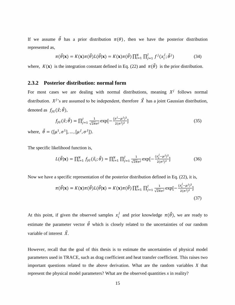
If we assume �� has a prior distribution 𝜋(𝜃) , then we have the posterior distribution

represented as,

𝜋(��|𝐱) = 𝐾(𝐱)𝜋(��)𝐿(��|𝐱) = 𝐾(𝐱)𝜋(��) ∏ 𝑁𝑖=1 ∏ 𝐽

𝑗=1 𝑓𝑗(𝑥𝑖𝑗; ��𝑗) (34)

where, 𝐾(𝐱) is the integration constant defined in Eq. (22) and 𝜋(��) is the prior distribution.

2.3.2 Posterior distribution: normal form

For most cases we are dealing with normal distributions, meaning 𝑋𝑗 follows normal

distribution. 𝑋𝑗’s are assumed to be independent, therefore �� has a joint Gaussian distribution,

denoted as 𝑓𝐽𝐺(��; ��),

𝑓𝐽𝐺(��; ��) = ∏ 𝐽𝑗=1

1

√2𝜋𝜎𝑗 exp[−(𝑥𝑗−𝜇𝑗)2

2(𝜎𝑗)2 ] (35)

where, �� = ([𝜇1, 𝜎1], … , [𝜇 𝐽, 𝜎𝐽]).

The specific likelihood function is,

𝐿(��|𝐱) = ∏ 𝑁𝑖=1 𝑓𝐽𝐺(��𝑖; ��) = ∏ 𝑁

𝑖=1 ∏ 𝐽𝑗=1

1

√2𝜋𝜎𝑗 exp[−(𝑥𝑖

𝑗−𝜇𝑗)2

2(𝜎𝑗)2 ] (36)

Now we have a specific representation of the posterior distribution defined in Eq. (22), it is,

𝜋(��|𝐱) = 𝐾(𝐱)𝜋(��)𝐿(��|𝐱) = 𝐾(𝐱)𝜋(��) ∏ 𝑁𝑖=1 ∏ 𝐽

𝑗=1

1

√2𝜋𝜎𝑗 exp[−(𝑥𝑖

𝑗−𝜇𝑗)2

2(𝜎𝑗)2 ]

(37)

At this point, if given the observed samples 𝑥𝑖𝑗 and prior knowledge 𝜋(��), we are ready to

estimate the parameter vector �� which is closely related to the uncertainties of our random

variable of interest ��.

However, recall that the goal of this thesis is to estimate the uncertainties of physical model

parameters used in TRACE, such as drag coefficient and heat transfer coefficient. This raises two

important questions related to the above derivation. What are the random variables X that

represent the physical model parameters? What are the observed quantities x in reality?

16

Since the physical model coefficients are our random variables of interest, it is clear that 𝑋𝑗

should represent these physical model coefficients. Ideally, we would like to observe the value of

these physical model coefficients, meaning 𝑥𝑖𝑗, in each specific experiment or calculation. In

practice, it is impossible to directly measure the physical model coefficients. A further step is

necessary to relate observable quantities to physical model coefficients ( 𝑋𝑗).

2.3.3 Application implementation

The output quantity that we can observe/calculate in an experiment/calculation is temperature,

void fraction and pressure drop. Mathematically, these output quantities are a deterministic

function of the physical model coefficients, which means that the output quantities contain the

same statistical information as the physical model coefficients in certain conditions. The

necessary conditions are described below.

Let 𝑌 denote experimentally observable output quantity, such as temperature, void fraction and

pressure drop. 𝑌 should be a deterministic function the physical model coefficient 𝑋, which

gives,

𝑌 = 𝑌(𝑋) (38)

The statement that 𝑌 contains the same information as 𝑋 means: if we have observed samples

𝐲, the following conditional distribution equation is correct under certain conditions,

𝜋(��|𝑥) = 𝜋(��|𝑦) (39)

The necessary condition is that the function 𝑌(𝑋) is invertible.

Now, let’s consider the multi-variable case, meaning 𝑌 is a function of vector ��,

𝑌 = 𝑌(��) (40)

where, following the previous notation, �� is a 𝐽-dimensional vector.

First let’s consider a simple case 𝐽 = 2 and then generalize the result to other dimension,

𝑌1 = 𝑌1(𝑋1, 𝑋2) (41)

and let’s assume 𝑌1 is a linear function of ��,

17

𝑌1 = 𝑌01 + 𝑎1,1(𝑋1 − 𝑥0

1) + 𝑎1,2(𝑋2 − 𝑥02) (42)

where, 𝑎1,1, 𝑎1,2 are used to denote the sensitivity coefficient of 𝑌 with respect to 𝑋1, 𝑋2, that

is 𝑎1,𝑗 =∂𝑌1

∂𝑋𝑗. 𝑥01, 𝑥0

2 are nominal values of 𝑋1, 𝑋2, respectively. It is clear that the assumption

shown in Eq. (42) can be derived from Taylor series expansion. Since 𝑥01, 𝑥0

2 are known

constants and 𝑎1,1, 𝑎1,2 are also known constants (obtained from sensitivity analysis), to

simplify the notation let’s absorb 𝑥01, 𝑥0

2 into constant 𝑌01, Eq. (42) simplifies to,

𝑌1 = 𝑌01 + 𝑎1,1𝑋1 + 𝑎1,2𝑋2 (43)

Note that 𝑌1 alone contains less information than 𝑋1, 𝑋2. In other words, it is not possible to

invert 𝑌1 to obtain 𝑋1, 𝑋2 . There are two ways to solve this problem, described in the

following two sections, 2.3.3.1 and 2.3.3.2.

2.3.3.1 MLE 1: multiple output variables

A possible solution is to have another random variable 𝑌2 that is also a deterministic function

of 𝑋1, 𝑋2. Following the same assumption as 𝑌1, 𝑌2 it simplifies to,

𝑌2 = 𝑌02 + 𝑎2,1𝑋1 + 𝑎2,2𝑋2 (44)

Then, the condition to invert Y becomes,

det𝐀 = det (𝑎1,1 𝑎1,2

𝑎2,1 𝑎2,2) ≠ 0 (45)

where 𝐀 is the sensitivity coefficient matrix. The condition shown in Eq. (45) means the

sensitivity coefficient matrix is invertible.

This is easier to generalize after rewriting Eqs. (43) and (44) in a matrix form,

�� = ��0 + 𝐀�� (46)

where, �� = (𝑌1, 𝑌2)T and ��0 = (𝑌01, 𝑌0

2)T.

Before continuing the derivation, it is useful to clarify 𝑌1 and 𝑌2. As said earlier, 𝑌1 and 𝑌2

are output quantities (observables) in a thermal-hydraulic experiment, such as temperature, void

fraction or pressure drop. The choice of 𝑌1 and 𝑌2 is not unique, but the condition shown in

Eq. (45) has to be satisfied and will be the main constraint in selecting 𝑌1 and 𝑌2 when the

18

inverse uncertainty algorithm is applied to a practical thermal-hydraulics problem.

Since �� contains the same information as ��, we have,

𝜋(��|��) = 𝜋(��|��) (47)

Because each component of �� follows a Gaussian distribution and each component of �� is a

linear combination of ��, �� follows a jointly Gaussian distribution. The following are the

statistical properties of ��,

��𝑥 = E(��) = (𝜇1

𝜇2) (48)

��𝑦 = E(��) = (𝑌0

1 + 𝑎1,1𝜇1 + 𝑎1,2𝜇2

𝑌02 + 𝑎2,1𝜇1 + 𝑎2,2𝜇2) (49)

𝚺𝑥 = cov(��, ��) = ((𝜎1)2 0

0 (𝜎2)2) (50)

𝚺𝑦 = cov(��, ��) = ((𝑎1,1)2(𝜎1)2 + (𝑎1,2)2(𝜎2)2 𝑎1,1𝑎2,1(𝜎1)2 + 𝑎1,2𝑎2,2(𝜎2)2

𝑎1,1𝑎2,1(𝜎1)2 + 𝑎1,2𝑎2,2(𝜎2)2 (𝑎2,1)2(𝜎1)2 + (𝑎2,2)2(𝜎2)2 )

(51)

Note that 𝑌1 and 𝑌2 are usually not independent.

Now we rewrite Eq. (48) – Eq. (51) into a matrix form as,

��𝑦 = ��0 + 𝐀��𝑥 (52)

𝚺𝑦 = 𝐀𝚺𝑥𝐀T (53)

and the joint distribution of �� is,

𝑓(��; ��) =1

2𝜋|𝚺𝑦|−

1

2exp[−1

2(�� − ��𝑦)T𝚺𝑦

−1(�� − ��𝑦)] (54)

To clarify, Table 1 gives a practical meaning of the most important variables.

19

Table 1 Practical meaning of important variables

Variables Meaning

�� input model parameter random variable

�� output random variable from experimental measurement

��0 output random variable from code prediction

�� random error of experimental measurement

𝐀 sensitivity coefficient matrix

𝜇𝑥, 𝚺𝑥 mean and covariance matrix of input model parameter random variable

𝜇𝑦, 𝚺𝑦 mean and covariance matrix of output random variable

𝜇𝑒 , 𝚺𝑒 mean and covariance matrix of random error of experimental measurement

Two additional considerations have to be made for completeness,

Random error: in the previous derivation, random error of an experimental measurement

is ignored. The random error is usually assumed to be mean-zero and does not depend on

�� or ��.

For different observed sample 𝑖, the sensitivity coefficient matrix and other quantities

might be different. This is modified in the following equations by consistently adding the

subscript 𝑖 to relevant quantities.

The previous equations now become,

��𝑖 = ��0,𝑖 + 𝐀𝑖�� + ��𝑖 (55)

��𝑦,𝑖 = ��0,𝑖 + 𝐀𝑖��𝑥 (56)

𝚺𝑦,𝑖 = 𝐀𝑖𝚺𝑥𝐀𝑖T + 𝚺𝑒,𝑖 (57)

𝑓𝑖(��; ��) =1

2𝜋|𝚺𝑦,𝑖|

−1

2exp[−1

2(�� − ��𝑦,𝑖)

T𝚺𝑦,𝑖−1(�� − ��𝑦,𝑖)] (58)

If there are 𝑁 sets of observed samples, the posterior distribution can be written as a function of

𝐲. The assumption is that ��𝑖’s are independent to each other,

𝐿1(��|𝐲) = ∏ 𝑁𝑖=1

1

2𝜋|𝚺𝑦,𝑖|

−1

2exp[−1

2(��𝑖 − ��𝑦,𝑖)

T𝚺𝑦,𝑖−1(��𝑖 − ��𝑦,𝑖)] (59)

𝜋1(��|𝐲) = 𝐾(𝐲)𝜋(��) ∏ 𝑁𝑖=1

1

2𝜋|𝚺𝑦,𝑖|

−1

2exp[−1

2(��𝑖 − ��𝑦,𝑖)

T𝚺𝑦,𝑖−1(��𝑖 − ��𝑦,𝑖)] (60)

The subscript 1 in the likelihood function and posterior distribution denotes MLE 1, the

subscript 𝑖 is used to denote 𝑖’th observed sample, while the superscript 𝑗 is used to denote

20

𝑗’th variable.

Eqs. (59) and (60) are the starting point for the following MLE, MAP and MCMC estimates.

2.3.3.2 MLE 2: assumption of independence between output variables

Though a single 𝑌1 has less information than 𝑋1, 𝑋2, we usually have more than one observed

value of 𝑌1 , that is we have 𝑌11, 𝑌2

1, ⋯ , 𝑌𝑁1 . These 𝑌𝑖

1 ’s contain enough information for

estimating 𝑋1, 𝑋2. The issue is that 𝑌𝑖1’s are correlated with each other and it is difficult to

obtain their joint distribution. In order to proceed, 𝑌𝑖1’s are assumed to be independent of each

other. Without confusion, let’s drop the superscript and denote the output variables as

𝑌1, 𝑌2, ⋯ , 𝑌𝑖, ⋯ , 𝑌𝑁, then,

𝑌𝑖 = 𝑌0,𝑖 + 𝐴𝑖�� + 𝐸𝑖 (61)

𝜇𝑦,𝑖 = 𝑌0,𝑖 + 𝐴𝑖𝜇𝑥 (62)

Σ𝑦,𝑖 = 𝐴𝑖Σ𝑥𝐴𝑖T + Σ𝑒,𝑖 (63)

𝑓𝑖(��; ��) =1

√2πΣ𝑦,𝑖exp[−

(𝑦𝑖−𝜇𝑦,𝑖)2

2Σ𝑦,𝑖] (64)

Note that the difference between Eqs. (55) – (58) and Eqs. (61) – (64) is that 𝐴𝑖 is now a vector.

The posterior distribution can be written as,

𝐿2(��|𝐲) = ∏ 𝑁𝑖=1

1

√2𝜋Σ𝑦,𝑖exp[−

(𝑦𝑖−𝜇𝑦,𝑖)2

2Σ𝑦,𝑖] (65)

𝜋2(��|𝐲) = 𝐾(𝐲)𝜋(��) ∏ 𝑁𝑖=1

1

√2𝜋Σ𝑦,𝑖exp[−

(𝑦𝑖−𝜇𝑦,𝑖)2

2Σ𝑦,𝑖] (66)

The subscript 2 in the likelihood function and posterior distribution denotes MLE 2.

2.3.3.3 Difference between MLE 1 and MLE 2

Though Eqs. (59) (60) and Eqs. (65) (66) have similar form, they are not identical because of the

additional assumption used to obtain Eqs. (65) (66). The difference is whether we deal with

multiple output variables (MLE 1) or single output variable (MLE 2). If we need to estimate 𝐽

model parameters, we need to provide 𝐽 output variables for solution of MLE 1 and a single

output variable for solution of MLE 2. The MLE 1 provides a chance to estimate the correlation

21

between different input model parameters. The capabilities and limitations of each model are

discussed when these two solutions are applied to numerical data.

2.4 Maximum Likelihood Estimation and

Expectation-Maximization algorithm

We will derive solution algorithm for MLE with MLE 1 Eq. (59) and then generalize the results

to MLE 2 by replacing vectors and matrixes with scalars and vectors, respectively.

The idea behind MLE is to maximize the likelihood function to solve for the parameter vector ��.

Though direction maximization could be done using for example Newton’s method, an

Expectation-Maximization (E-M) algorithm (Malachlan, 2007) (Shrestha, 2015) is usually

applied to maximize the likelihood function. There are 2 steps in E-M algorithm,

Maximization. Assuming the covariance matrix 𝚺𝑥 is known, ��𝑥 could be solved by

maximize the likelihood function.

��𝑥,new = max��𝑥

𝐿1(��|𝐲) (67)

Expectation. Once the ��𝑥 is obtained, the covariance matrix 𝚺𝑥 can be updated using

conditional expectation.

𝚺𝑥,new = E[(�� − ��𝑥,new)(�� − ��𝑥,new)T|𝐲] (68)

The reason that E-M algorithm works is that the likelihood is guaranteed to increase.

Since maximizing the logarithm of the likelihood function is the same as maximizing the

likelihood function itself, it is easier to proceed with maximizing the logarithm of the likelihood

function, called log-likelihood,

log𝐿1(��|𝐲) = ∑ 𝑁𝑖=1 [−

1

2log|𝚺𝑦,𝑖| − log2𝜋 −

1

2(��𝑖 − ��𝑦,𝑖)

T𝚺𝑦,𝑖−1(��𝑖 − ��𝑦,𝑖)] (69)

2.4.1 Maximization step

Note that the log-likelihood in Eq. (69) is a quadratic function of ��𝑥 due to the particular

properties of Gaussian distribution. By taking a derivative of the log-likelihood with respect to

22

��𝑥 and setting it equal be zero, we get a system of linear equations for solving ��𝑥,

∂log𝐿1(��|𝐲)

∂��𝑥= 0 (70)

which gives,

𝐌𝐿��𝑥 = ��𝐿 (71)

where,

𝐌𝐿 = (∑ 𝑁

𝑖=1 (𝑎1,1,𝑖, 𝑎2,1,𝑖)𝚺𝑦,𝑖−1(𝑎1,1,𝑖, 𝑎2,1,𝑖)

T ∑ 𝑁𝑖=1 (𝑎1,1,𝑖, 𝑎2,1,𝑖)𝚺𝑦,𝑖

−1(𝑎1,2,𝑖, 𝑎2,2,𝑖)T

∑ 𝑁𝑖=1 (𝑎1,2,𝑖, 𝑎2,2,𝑖)𝚺𝑦,𝑖

−1(𝑎1,1,𝑖, 𝑎2,1,𝑖)T ∑ 𝑁

𝑖=1 (𝑎1,2,𝑖, 𝑎2,2,𝑖)𝚺𝑦,𝑖−1(𝑎1,2,𝑖, 𝑎2,2,𝑖)

T)

(72)

��𝐿 = (∑ 𝑁

𝑖=1 (𝑎1,1,𝑖, 𝑎2,1,𝑖)𝚺𝑦,𝑖−1(��𝑖 − ��0,𝑖)

∑ 𝑁𝑖=1 (𝑎1,1,𝑖, 𝑎2,1,𝑖)𝚺𝑦,𝑖

−1(��𝑖 − ��0,𝑖)) (73)

In the matrix form,

𝐌𝐿 = ∑ 𝑁𝑖=1 𝐀𝑖

T𝚺𝑦,𝑖−1𝐀𝑖 (74)

��𝐿 = ∑ 𝑁𝑖=1 𝐀𝑖

T𝚺𝑦,𝑖−1(��𝑖 − ��0,𝑖) (75)

An update to ��𝑥 is obtained by solving Eq. (71).

2.4.2 Expectation step

Since the mean vector ��𝑥 has been updated, the expectation step updates the covariance matrix

of 𝑋 conditioned on the observed output 𝑌,

(𝜎𝑗)new2 = E[(𝑋𝑗 − 𝜇𝑗)2|��𝑖] (76)

= E[(𝑋𝑗 − ��𝑗 + ��𝑗 − 𝜇𝑗)2|��𝑖]

= E[(𝑋𝑗 − ��𝑗)2|��𝑖] + E[(��𝑗 − 𝜇𝑗)2|��𝑖] + E[(𝑋𝑗 − ��𝑗)(��𝑗 − 𝜇𝑗)|��𝑖]

where, ��𝑗 is the linear MMSE of 𝑋𝑗 conditioned on ��𝑖.

Using the properties of linear MMSE, we have,

��𝑗 = cov[𝑋𝑗 , ��𝑖]cov[��𝑖, ��𝑖]−1(��𝑖 − ��𝑦,𝑖) + 𝜇𝑗 (77)

E[(𝑋𝑗 − ��𝑗)2|��𝑖] = cov[𝑋𝑗 , 𝑋𝑗] − cov[𝑋𝑗 , ��𝑖]cov[��𝑖, ��𝑖]−1cov[��𝑖, 𝑋𝑗] (78)

E[(��𝑗 − 𝜇𝑗)2|��𝑖] = {cov[𝑋𝑗 , ��𝑖]cov[��𝑖 , ��𝑖]−1(��𝑖 − ��𝑦,𝑖)}2 (79)

E[(𝑋𝑗 − ��𝑗)(��𝑗 − 𝜇𝑗)|��𝑖] = 0 (80)

23

Using the above substitutions, we get,

(𝜎𝑗)new2 = (𝜎𝑗)old

2 − cov[𝑋𝑗 , ��𝑖]cov[��𝑖, ��𝑖]−1cov[��𝑖, 𝑋𝑗] + {cov[𝑋𝑗 , ��𝑖]cov[��𝑖, ��𝑖]

−1(��𝑖 −

��𝑦,𝑖)}2 (81)

Since we have 𝑁 sets of observed output, the effect of each set could be added to the update of

the covariance matrix by a simple average,

(𝜎𝑗)new2 = (𝜎𝑗)old

2

+1

𝑁∑ 𝑁

𝑖=1 (−cov[𝑋𝑗 , ��𝑖]cov[��𝑖, ��𝑖]−1cov[��𝑖, 𝑋𝑗] + {cov[𝑋𝑗 , ��𝑖]cov[��𝑖, ��𝑖]

−1(��𝑖 − ��𝑦,𝑖)}2) (82)

With the help of two new covariance matrixes, Eq. (82) could be written in a matrix form,

𝚺𝑥𝑦,𝑖 = cov(��, ��𝑖) = 𝐀𝑖𝚺𝑥 (83)

𝐝𝚺𝑥 = ∑ 𝑁𝑖=1 (−𝚺𝑥𝑦,𝑖

T 𝚺𝑦,𝑖−1𝚺𝑥𝑦,𝑖 + [𝚺𝑥𝑦,𝑖

T 𝚺𝑦,𝑖−1(��𝑖 − ��𝑦,𝑖)][𝚺𝑥𝑦,𝑖

T 𝚺𝑦,𝑖−1(��𝑖 − ��𝑦,𝑖)]T)

(84)

𝚺𝑥,new = 𝚺𝑥,old +1

𝑁diag(𝐝𝚺𝑥) (85)

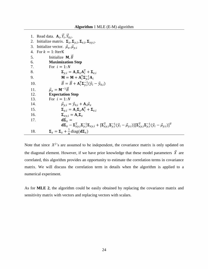
Algorithm 1 shows the MLE algorithm.

24

Algorithm 1 MLE (E-M) algorithm

1. Read data. 𝐀𝑖, ��𝑖, ��0,𝑖.

2. Initialize matrix. 𝚺𝑥, 𝚺𝑦,𝑖, 𝚺𝑒,𝑖, 𝚺𝑥𝑦,𝑖.

3. Initialize vector. ��𝑥, ��𝑦,𝑖

4. For 𝑘 = 1: IterK

5. Initialize 𝐌, ��

6. Maximization Step

7. For 𝑖 = 1: 𝑁

8. 𝚺𝑦,𝑖 = 𝐀𝑖𝚺𝑥𝐀𝑖T + 𝚺𝑒,𝑖

9. 𝐌 = 𝐌 + 𝐀𝑖T𝚺𝑦,𝑖

−1𝐀𝑖

10. �� = �� + 𝐀𝑖T𝚺𝑦,𝑖

−1(��𝑖 − ��0,𝑖)

11. ��𝑥 = 𝐌−1��

12. Expectation Step

13. For 𝑖 = 1: 𝑁

14. ��𝑦,𝑖 = ��0,𝑖 + 𝐀𝑖��𝑥

15. 𝚺𝑦,𝑖 = 𝐀𝑖𝚺𝑥𝐀𝑖T + 𝚺𝑒,𝑖

16. 𝚺𝑥𝑦,𝑖 = 𝐀𝑖𝚺𝑥

17. 𝐝𝚺𝑥 =

𝐝𝚺𝑥 − 𝚺𝑥𝑦,𝑖T 𝚺𝑦,𝑖

−1𝚺𝑥𝑦,𝑖 + [𝚺𝑥𝑦,𝑖T 𝚺𝑦,𝑖

−1(��𝑖 − ��𝑦,𝑖)][𝚺𝑥𝑦,𝑖T 𝚺𝑦,𝑖

−1(��𝑖 − ��𝑦,𝑖)]T

18. 𝚺𝑥 = 𝚺𝑥 +1

𝑁diag(𝐝𝚺𝑥)

Note that since 𝑋𝑗’s are assumed to be independent, the covariance matrix is only updated on

the diagonal element. However, if we have prior knowledge that these model parameters �� are

correlated, this algorithm provides an opportunity to estimate the correlation terms in covariance

matrix. We will discuss the correlation term in details when the algorithm is applied to a

numerical experiment.

As for MLE 2, the algorithm could be easily obtained by replacing the covariance matrix and

sensitivity matrix with vectors and replacing vectors with scalars.

25

2.5 Maximum A Posterior (MAP) algorithm

The main idea behind MAP is to maximize the posterior distribution for solving the parameter

vector ��. The difference between the likelihood function and the posterior distribution is the

prior distribution 𝜋(��) and a constant 𝐾(𝐲). Using the concept of Expectation-Maximization,

the MAP solution algorithm is derived in a similar way, by adding the effect of the prior

distribution.

Let 𝐌𝜋, ��𝜋 be the coefficient matrix and source vector due to the effect of prior distribution,

respectively. 𝐌𝜋, ��𝜋 could be obtained by differentiating the logarithm of prior distribution. For

example, if the normal-inverse gamma prior distribution is used, 𝐌𝜋, ��𝜋 will be used in the

maximization step for solving ��𝑥 as,

𝐌𝜋 = diag(𝑘1

(𝜎1)2 , ⋯ ,𝑘𝑗

(𝜎𝑗)2 , ⋯ ,𝑘𝐽

(𝜎𝐽)2) (86)

��𝜋 = [𝑘1𝛽1

(𝜎1)2 , ⋯ ,𝑘𝑗𝛽𝑗

(𝜎𝑗)2 , ⋯ ,𝑘𝐽𝛽𝐽

(𝜎𝐽)2]T (87)

Using these correction terms, the MAP’s version of the coefficient matrix and source vector for

solving 𝜇𝑥 becomes,

𝐌𝑝 = 𝐌𝐿 + 𝐌𝜋 (88)

��𝑝 = ��𝐿 + ��𝜋 (89)

where, the subscript 𝑝 denotes posterior distribution. Then the MAP algorithm is shown in

Algorithm 2.

26

Algorithm 2 MAP (E-M) algorithm

1. Read data. 𝐀𝑖, ��𝑖, ��0,𝑖.

2. Initialize matrix. 𝚺𝑥, 𝚺𝑦,𝑖, 𝚺𝑒,𝑖, 𝚺𝑥𝑦,𝑖.

3. Initialize vector. ��𝑥, ��𝑦,𝑖

4. Choose a prior distribution.

5. For 𝑘 = 1: IterK

6. Initialize 𝐌, 𝐌𝜋, ��, ��𝜋

7. Maximization Step

8. For 𝑖 = 1: 𝑁

9. 𝚺𝑦,𝑖 = 𝐀𝑖𝚺𝑥𝐀𝑖T + 𝚺𝑒,𝑖

10. 𝐌 = 𝐌 + 𝐀𝑖T𝚺𝑦,𝑖

−1𝐀𝑖

11. �� = �� + 𝐀𝑖T𝚺𝑦,𝑖

−1(��𝑖 − ��0,𝑖)

12. 𝐌 = 𝐌 + 𝐌𝜋

13. �� = �� + ��𝜋

14. ��𝑥 = 𝐌−1��

15. Expectation Step

16. For 𝑖 = 1: 𝑁

17. ��𝑦,𝑖 = ��0,𝑖 + 𝐀𝑖��𝑥

18. 𝚺𝑦,𝑖 = 𝐀𝑖𝚺𝑥𝐀𝑖T + 𝚺𝑒,𝑖

19. 𝚺𝑥𝑦,𝑖 = 𝐀𝑖𝚺𝑥

20. 𝐝𝚺𝑥 =

𝐝𝚺𝑥 − 𝚺𝑥𝑦,𝑖T 𝚺𝑦,𝑖

−1𝚺𝑥𝑦,𝑖 + [𝚺𝑥𝑦,𝑖T 𝚺𝑦,𝑖

−1(��𝑖 − ��𝑦,𝑖)][𝚺𝑥𝑦,𝑖T 𝚺𝑦,𝑖

−1(��𝑖 − ��𝑦,𝑖)]T

21. 𝚺𝑥 = 𝚺𝑥 +1

𝑁diag(𝐝𝚺𝑥)

2.6 Markov Chain Monte Carlo (MCMC) Recall that the MLE and MAP algorithms developed thus far are based on the particular

properties of the normal distribution, the conjugate distribution and the linearity assumption. If

any of these conditions are not satisfied, the application of MLE and MAP would be difficult

because we would not be able to obtain an explicit analytical form of the likelihood function and

posterior distribution. The MCMC process solves this problem.

Recall that the posterior distribution 𝜋(��|𝐲) can be generalized as the following form,

𝜋(��|𝐲) = 𝐾(𝐲)𝜋(��)𝐿(��|𝐲) (90)

However, difficulties exist in calculating 𝐾(𝐲), 𝜋(��) and 𝐿(��|𝐲) when the distribution of 𝑌

and the posterior distribution is general:

𝐿(��|𝐲). Recall that in the derivation of MLE and MAP, 𝑋 is assumed to follow a

27

Gaussian distribution and thus 𝑌 also follows a Gaussian distribution with an additional

linearity assumption. If these assumptions are not satisfied, analytical maximization of

the likelihood function becomes impossible.

𝜋(��). In the previous derivation, 𝜋(𝜃) is differentiable in real space 𝑅 or positive real

space 𝑅+ to ensure that the analytical differentiation is possible. However, in practice

the parameter vector might only be physical on a certain interval. For example, in

estimating a model parameter (e.g. subcooled boiling heat transfer coefficient), we have

prior knowledge that the correct value of this model parameter should be close to the

nominal value used in the code and should always be positive, but this prior knowledge is

difficult to be considered in MLE and MAP algorithm.

𝐾(𝐲). Unless a conjugate prior distribution is used, which depends on the distribution

family of 𝑋, the constant 𝐾(𝐲) is obtained with a multi-dimensional integration as

given in Eq. (22). This integration is both analytically and numerically difficult.

These difficulties can be overcome using MCMC process. The idea behind MCMC is to sample

the posterior distribution without knowledge of the explicit form of the posterior distribution.

This sampling is implemented by using an iterative Monte Carlo sampling, which usually forms

a Markov Chain. We need to devise an aperiodic and irreducible Markov Chain that converges to

the posterior distribution of interest, that is to devise the probability transition matrix 𝐏.

Many sampling methods exist, such as Metropolis-Hastings sampling, Gibbs sampling and other

advanced methods (Gilks, 2005). Among these methods, Metropolis-Hastings sampling (Chib,

1995) has the least requirements on the posterior distribution and will be used in this thesis.

Metropolis-Hastings algorithm

Let’s start with a posterior distribution 𝜋(𝜃|𝐲) which only has a scalar parameter 𝜃. In order to

proceed, a proposal distribution 𝑔(𝜉|𝜃𝑘) is needed, where 𝜉 is a dummy variable used to

denote a random process. This proposal distribution gives the rule of how the Markov Chain

proceeds given a current state 𝜃𝑘. The Metropolis-Hastings algorithm proceeds in three main

steps:

28

1. Sample a proposal variable 𝜉 from 𝑔(𝜉|𝜃𝑘).

2. Calculate the acceptance probability.

𝑟(𝜉, 𝜃𝑘) = min{1,𝜋(𝜉|𝐲)𝑔(𝜃𝑘|𝜉)

𝜋(𝜃𝑘|𝐲)𝑔(𝜉|𝜃𝑘)} (91)

3. Accept (𝜃𝑘+1 = 𝜉) or drop (𝜃𝑘+1 = 𝜃𝑘) with probability 𝑟(𝜉, 𝜃𝑘).

The following Algorithm 3 shows these steps.

Algorithm 3 Metropolis-Hastings algorithm: 1-D

1. Initialize 𝜃0.

2. Choose the proposal distribution.

3. For 𝑘 = 0: IterK

4. Sample a proposal variable 𝜉 from 𝑔(𝜉|𝜃𝑘).

5. Calculate the accept probability. 𝑟 = min{1,𝜋(𝜉|𝐲)𝑔(𝜃𝑘|𝜉)

𝜋(𝜃𝑘|𝐲)𝑔(𝜉|𝜃𝑘)}

6. Sample a uniformly distributed random variable 𝜂 in [0,1].

7. If (𝜂 < 𝑟), 𝜃𝑘+1 = 𝜉; else continue.

The algorithm could be different for different forms of posterior distribution and choice of

proposal distribution. If the proposal distribution were close to the posterior distribution, the

algorithm would be more efficient because more proposed random variables would be accepted.

For multi-dimensional parameter vector ��, �� can be sampled element by element using the

Metropolis-Hastings algorithm:

1. Sample a proposal variable 𝜉𝑚 from 𝑔𝑚(𝜉|𝜃𝑘,𝑚).

2. Update the proposal element 𝜉𝑚 to the mth

element of parameter vector ��𝑘 as 𝜉,

𝜉 = (𝜃𝑘,1, 𝜃𝑘,2, ⋯ , 𝜉𝑚, 𝜃𝑘,𝑚+1, ⋯ ) (92)

3. Calculate the acceptance probability.

𝑟(𝜉, ��𝑘) = min{1,𝜋(��|𝐲)𝑔𝑚(𝜃𝑘,𝑚|𝜉𝑚)

𝜋(��𝑘|𝐲)𝑔𝑚(𝜉𝑚|𝜃𝑘,𝑚)} (93)

4. Accept (𝜃𝑘+1,𝑚 = 𝜉𝑚) or drop (𝜃𝑘+1,𝑚 = 𝜃𝑘,𝑚) with probability 𝑟(𝜉, ��𝑘).

The multi-dimensional version of the sampling algorithm is shown in the following Algorithm

4.

29

Algorithm 4 Metropolis-Hastings algorithm: Multi-dimensional

1. Initialize ��0.

2. Choose the proposal distribution.

3. For 𝑘 = 0: IterK

4. For 𝑚 = 1: M

5. Sample a proposal variable 𝜉𝑚 from 𝑔𝑚(𝜉|𝜃𝑘,𝑚).

6. Update the mth

element of ��𝑘 with 𝜉𝑚 as 𝜉.

7. Calculate the accept probability. 𝑟 = min{1,𝜋(��|𝐲)𝑔𝑚(𝜃𝑘,𝑚|𝜉𝑚)

𝜋(��𝑘|𝐲)𝑔𝑚(𝜉𝑚|𝜃𝑘,𝑚)}

8. Sample a uniformly distributed random variable 𝜂 in [0,1].

9. If (𝜂 < 𝑟), 𝜃𝑘+1,𝑚 = 𝜉𝑚; else continue.

2.7 Summary of Chapter 2

In this chapter, detailed derivation is provided for the Maximum Likelihood Estimation (MLE),

Maximum A Posterior (MAP) method and Expectation-Maximization (E-M) algorithms. In

addition, the concept of Markov Chain Monte Carlo (MCMC) and the Metropolis-Hastings

sampling method for MCMC is provided.

Variations on these algorithms include different methods of processing output variables (single

or multiple), output correlations (independent or correlated) and prior distributions (none,

conjugate, non-informative or uniform). A summary of possible variations and their capabilities

are listed in Table 2.

Table 2 Summary of various algorithms

Algorithms Output variables Output Correlation Prior distribution

MLE 1a multiple independent N/A

MLE 1b multiple correlated N/A

MLE 2 single independent N/A

MAP 1 multiple correlated conjugate

MAP 2 single independent conjugate

MCMC 1 multiple independent non-informative

MCMC 2 multiple independent conjugate

MCMC 3 multiple independent uniform

In the following Chapters, we will test these algorithms with numerical data (with known

solution) and then apply them to an experimental benchmark (without known solution).

30

3 Numerical tests

Before the algorithms are applied to an experimental benchmark data, we will first test the three

algorithms (MLE, MAP, MCMC) with a set of numerical data.

3.1 Numerical data

Recall from Table 1, a numerical data set (��𝑖, ��0,𝑖, 𝐀𝑖, ��𝑖) is needed as input to the algorithm.

The input random variable �� is to be estimated. For the numerical test the distribution of �� is

known. Then, (��𝑖, ��0,𝑖, 𝐀𝑖 , ��𝑖) will be generated randomly and related to ��. Table 3 summarizes

how the data are generated.

Table 3 Creation of data for the numerical test of MLE, MAP, MCMC

Variables Meaning Data

�� input model parameter sampled from (��𝑥, 𝚺𝑥)

��𝑖 error from experiment measurement sampled uniformly from 𝜀0 ∗ [−0.5,0.5]

𝚺𝑒,𝑖 covariance matrix of error 1/12 ∗ 𝜀02 ∗ 𝐈

𝐀𝑖 sensitivity coefficient matrix sampled uniformly from 𝑎0 ∗ [−0.5,0.5]

��0,𝑖 output from code prediction sampled uniformly from 𝑦0 ∗ [−0.5,0.5]

��𝑖 output from experiment measurement ��𝑖 = ��0,𝑖 + 𝐀𝑖��𝑖 + ��𝑖

In Table 3, 𝜀0, 𝑎0, 𝑦0 are used to denote the intensity of these random variables. By adjusting

𝜀0, 𝑎0, 𝑦0 and ��𝑥, 𝚺𝑥 , various numerical data can be produced. For testing purposes, three

primarily set of data are created using the parameters shown in Table 4.

31

Table 4 Numerical data sets

Variables DATA-I DATA-II DATA-III

�� Independent Gaussian Correlated Gaussian Independent Uniform

𝜇𝑥 ± ��𝑥 −2.0 ± 2.0 −2.0 ± 2.0 −2.0 ± 2.0

2.0 ± 4.0 2.0 ± 4.0 2.0 ± 4.0 Correlation 0.0 0.5 0.0

𝜀0 2.0 2.0 2.0

𝑎0 5.0 5.0 5.0

𝑦0 10.0 10.0 10.0

(𝑁, 𝐽) (100,2) (100,2) (100,2)

As shown in Table 4, DATA-I and DATA-II are created using jointly Gaussian distributions

without and with correlation, respectively; DATA-III is created using an independent uniform

distribution, which should be difficult to estimate using both MLE and MAP algorithm. Note that

the ratio of 𝜀0 to 𝑦0 represents the relative error of the measurement, which could be freely

adjusted.

3.2 MLE test results

After applying the MLE algorithm to the three sets of data, the statistical properties of the input

data X are estimated (Table 5). All iterations were started with a zero mean vector and identity

covariance matrix.

Table 5 Comparison of estimated solutions from different MLE algorithms

Algorithm Variables DATA-I DATA-II DATA-III

Exact

�� Independent

Gaussian

Correlated

Gaussian Independent Uniform

��𝑥 ± ��𝑥 −2.0 ± 2.0 −2.0 ± 2.0 −2.0 ± 2.0

2.0 ± 4.0 2.0 ± 4.0 2.0 ± 4.0

correlation 0.0 0.5 0.0

MLE 1a ��𝑥 ± ��𝑥

-2.27 ± 2.07 -2.28 ± 2.05 -1.87 ± 2.10

1.60 ± 3.87 1.41 ± 4.05 2.06 ± 4.04

correlation N/A N/A N/A

MLE 1b ��𝑥 ± ��𝑥

-2.27 ± 2.07 -2.28 ± 2.07 -1.86 ± 2.10

1.60 ± 3.87 1.41 ± 4.09 2.06 ± 4.04

correlation 0.03 0.57 -0.03

MLE 2 ��𝑥 ± ��𝑥

-2.14 ± 1.73 -2.17 ± 1.66 -1.70 ± 2.12

1.47 ± 4.20 1.17 ± 4.22 2.23 ± 4.10

correlation N/A N/A N/A

32

Figure 1 shows how the likelihood function converges with the E-M iterations for DATA-II, the

convergence profile is similar for other data set. Figure 2 shows the comparison between

estimated solutions of different data sets and algorithms. Based on the likelihood convergence

profile and the estimate results comparison, the following statements can be made,

The likelihood function. Regardless of different solution algorithms and different data sets,

the likelihood function is increasing monotonically with the E-M iteration. This is desired

behavior because we want to maximize the likelihood function, which verifies the

reliability of the algorithms. For the data sets used, the likelihood function converges to a

maximum after about 20 E-M iterations, the number of iterations depends on specific

data.

The mean value estimation. Regardless of different solution algorithms and different data

sets, the mean values are estimated consistently close to the exact solution (-2.0, 2.0). The

deficiency in the estimation of different solution algorithm comes from the random error

(𝜀0) and the limited number of data (𝑁).

The covariance matrix estimation. Regardless of different solution algorithms and

different data sets, the variances are estimated close to the exact variances (4.0, 16.0).

However, the estimation of MLE 1a, 1b is better than the estimation of MLE 2. Besides,

MLE 1a, 2 are not capable of estimating the correlation terms, while MLE 1b finds the

correlation terms very well. The MLE 1b is better compared with MLE 1a.

The random error. For the purpose of this study the correct (exact) covariance matrix of

the error is used when the algorithms are applied to the data. If the information about the

error is incorrect or not known, the estimation of the covariance matrix (𝚺𝑥) of input

model parameters will be worse.

33

Figure 1 Likelihood function convergence of DATA-II: MLE test

Figure 2 Comparison between estimated solutions of different algorithms with DATA-II

3.3 MAP test results

3.3.1 Prior distribution

As mentioned earlier, a conjugate prior distribution is chosen for the MAP algorithm. Since �� is

assumed to be jointly Gaussian distribution, the prior distribution is chosen to be normal-inverse

gamma distribution,

0 2 4 6 8 10 12 14 16 18 200.84

0.86

0.88

0.9

0.92

0.94

0.96

0.98

1

1.02

E-M iteration

No

rm

ali

zed

lik

eli

ho

od

DATA-II: MLE test (Likelihoood) convergence

MLE 1a

MLE 1b

MLE 2

1 2-2.5

-2

-1.5

-1

-0.5

0

0.5

1

1.5

2

x: mean value of X

Est

ima

ted

mea

n v

alu

e

DATA2: MLE (mean value estimation)

Exact

MLE 1a

MLE 1b

MLE 2

1 20

2

4

6

8

10

12

14

16

18

x: variance X

Est

ima

ted

va

ria

nce

DATA2: MLE (variance estimation)

Exact

MLE 1a

MLE 1b

MLE 2

34

𝜋(��) ∝ ∏ 𝐽𝑗=1 [(𝜎𝑗)2]−[(𝑟𝑗+1)/2+1]exp{−

1

2(𝜎𝑗)2 [𝑘𝑗(𝜇𝑗 − 𝛽𝑗)2 + 𝜆𝑗]} (94)

Our prior knowledge is indicated by the hyperparameters (𝑟𝑗 , 𝑘𝑗 , 𝛽𝑗 , 𝜆𝑗). For example, 𝛽𝑗 and

𝜆𝑗

𝑟𝑗−2 is our prior knowledge of the expected value of 𝜇𝑗 and (𝜎𝑗)2. Usually 𝑟𝑗 is chosen to be

3, thus 𝜆𝑗 is the expectation value of (𝜎𝑗)2. Table 6 gives the values of the hyperparameters

used in the following MAP calculations.

Table 6 Hyperparameter values used in MAP estimates

Variables Meaning Value

𝑟 shape factor of normal-inverse gamma distribution (3, 3)T

�� shape factor of normal-inverse gamma distribution (1.0, 1.0)T

𝛽 expectation value of prior �� (−2.0, 2.0)T

𝜆 expectation value of prior ��2 (4.0, 16.0)T

Note that exact value of the mean and variance of �� is used for 𝛽 and 𝜆.

3.3.2 Estimation results

Using the hyperparameters given in Table 6, the MAP algorithm is applied to the data sets and

the estimation results are shown in Table 7.

Table 7 Comparison of estimated solutions with different MAP algorithms

Algorithm Variables DATA-I DATA-II DATA-III

Exact

�� Independent

Gaussian

Correlated

Gaussian

Independent

Uniform

��𝑥 ± ��𝑥 −2.0 ± 2.0 −2.0 ± 2.0 −2.0 ± 2.0

2.0 ± 4.0 2.0 ± 4.0 2.0 ± 4.0

Correlation 0.0 0.5 0.0

MAP 1 ��𝑥 ± ��𝑥

-2.26 ± 2.04 -2.27 ± 2.04 -1.86 ± 2.07

1.61 ± 3.81 1.42 ± 4.03 2.06 ± 3.98

Correlation 0.03 0.58 -0.03

MAP 2 ��𝑥 ± ��𝑥

-2.14 ± 1.71 -2.17 ± 1.63 -1.71 ± 2.09

1.47 ± 4.13 1.17 ± 4.16 2.23 ± 4.04

Correlation N/A N/A N/A

The results show that the estimation results from MAP algorithm are close to the exact solution.

35

MAP 2 results have larger error on the estimation than MAP 1, just like what was observed with

the MLE algorithm.

3.4 MCMC test results

As was described in Section 2.6, MCMC algorithm requires a prior distribution, likelihood

function and a proposal distribution.

3.4.1 Proposal distribution

The proposal distribution affects the efficiency of the sampling scheme, which means that if the

proposal distribution is close to the posterior distribution, the sampling scheme is more efficient

because more sampled data will be accepted. However, for the purpose of this thesis, the

efficiency of the sampling scheme is not the goal. To simplify the problem, the proposal

distribution is chosen to be a Gaussian distribution,

𝑔(𝜉|𝜃𝑘)~𝑁(𝜃𝑘 , 𝜎2) (95)

where 𝜎2 is the variance data sampled at the previous step. This proposal distribution is also

called the independent proposal distribution, because

𝑔(𝜃𝑘|𝜉)

𝑔(𝜉|𝜃𝑘)= 1 (96)

3.4.2 Prior distribution

Three types of prior distribution mentioned in Section 2.2 are tested, including non-informative

prior, conjugate prior and general prior. Table 8 summarizes the prior distributions used in

this thesis.

Table 8 Prior distribution used in MCMC test

Algorithms Prior type Prior distribution

MCMC 1 Non-informative 𝜋(��) = ∏ 𝐽𝑗=1

1

(𝜎𝑗)2

MCMC 2 Conjugate 𝜋(��) ∝ ∏ 𝐽𝑗=1 [(𝜎𝑗)2]−[(𝑟𝑗+1)/2+1]exp{−

1

2(𝜎𝑗)2[𝑘𝑗(𝜇𝑗 −

𝛽𝑗)2 + 𝜆𝑗]}

MCMC 3 Uniform 𝜃𝑘 distribute uniformly in [𝑎𝑘, 𝑏𝑘]

The conjugate prior distribution is chosen to be the same as the prior distribution used in the

MAP algorithm. For general prior distribution, a multi-variable uniform distribution is chosen. A

36

uniform distribution is chosen due to the fact that we might have a prior knowledge that the

model parameters of interest only exist in a certain interval. In this MCMC test, because the

exact mean values are (−2.0, 2.0) and variances are (4.0, 16.0), [𝑎𝑘, 𝑏𝑘] is chosen to be

[−4.0, 4.0] and [0, 36], respectively.

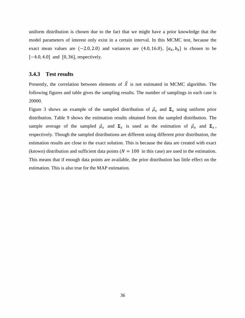
3.4.3 Test results

Presently, the correlation between elements of �� is not estimated in MCMC algorithm. The

following figures and table gives the sampling results. The number of samplings in each case is

20000.

Figure 3 shows an example of the sampled distribution of ��𝑥 and 𝚺𝑥 using uniform prior

distribution. Table 9 shows the estimation results obtained from the sampled distribution. The

sample average of the sampled ��𝑥 and 𝚺𝑥 is used as the estimation of ��𝑥 and 𝚺𝑥 ,

respectively. Though the sampled distributions are different using different prior distribution, the

estimation results are close to the exact solution. This is because the data are created with exact

(known) distribution and sufficient data points (𝑁 = 100 in this case) are used in the estimation.

This means that if enough data points are available, the prior distribution has little effect on the

estimation. This is also true for the MAP estimation.

37

Figure 3 Sampled distribution of θ using uniform prior distribution for DATA-II

Table 9 Comparison between estimated solutions with different MCMC algorithms

Algorithm Variables DATA-I DATA-II DATA-III

Exact

�� Independent

Gaussian

Correlated

Gaussian Independent Uniform

��𝑥 ± ��𝑥 −2.0 ± 2.0 −2.0 ± 2.0 −2.0 ± 2.0

2.0 ± 4.0 2.0 ± 4.0 2.0 ± 4.0

correlation 0.0 0.5 0.0

MCMC 1 ��𝑥 ± ��𝑥

-2.26 ± 2.11 -2.29 ± 2.08 -1.5 ± 2.14

1.58 ± 3.92 1.41 ± 4.12 2.08 ± 4.09

correlation N/A N/A N/A

MCMC 2 ��𝑥 ± ��𝑥

-2.26 ± 2.07 -2.28 ± 2.04 -1.86 ± 2.10

1.60 ± 3.87 1.41 ± 4.05 2.04 ± 4.04

correlation N/A N/A N/A

MCMC 3 ��𝑥 ± ��𝑥

-2.26 ± 2.13 -2.28 ± 2.11 -1.88 ± 2.17

1.60 ± 3.97 1.43 ± 4.17 2.06 ± 4.15

correlation N/A N/A N/A

-4 -3 -2 -10

1000

2000

3000

4000

x,1

Co

un

t

-2 0 2 40

1000

2000

3000

4000

x,2

Co

un

t

2 4 6 8 100

1000

2000

3000

4000

2

x,1

Co

un

t

10 20 30 400

1000

2000

3000

4000

2

x,2

Co

un

t

38

3.5 Summary of Chapter 3

In this chapter, three data sets with different distribution were created for testing purposes. The

data sets were created to be as practical and comprehensive as possible by considering different

distribution types, correlation between variables and the error (or noise) found in real data. These

data points were then used in testing MLE, MAP and MCMC algorithms.

For these data sets, estimations by all three types of algorithm (MLE, MAP and MCMC)were

reasonably close to the exact solution, however some algorithms may have larger differences

between the exact and estimated solution. For example, MLE, MAP 1a, 2 and MCMC

algorithms are not capable of estimating the correlation between variables, whereas MCMC is

capable of estimating a general prior distribution, which is very useful when the algorithm is

applied to practical data.

In terms of the estimation results, no significant difference was observed between different

algorithms, because sufficient data points were used. In other words, prior knowledge is not the

most significant criterion if the number of data points is large enough.

39

4 Application to BFBT benchmark

One of the most valuable publicly available databases for the thermal-hydraulics modeling of

BWR channels is the OECD/NEA BWR Full-size Fine-mesh Bundle Test (BFBT) benchmark,

which includes sub-channel void fraction measurements in a representative BWR fuel assembly

(Neykov, 2006). In this chapter, the BFBT benchmark data will be used to conduct inverse

uncertainty quantification of physical model parameters in the thermal-hydraulics code system

TRACE, using methods developed in previous Chapters. Then, the results will be validated by a

forward uncertainty propagation analysis using the probability density functions obtained from

the inverse uncertainty quantification.

This Chapter is organized to follow the order of performed the analysis:

Section 4.1: Description of BFBT benchmark.

Section 4.2: Accuracy analysis (AA) of TRACE prediction.

Section 4.3: Sensitivity analysis (SA) (Gajev, 2014) of model parameters.

Section 4.4: Validation of linearity assumption.

Section 4.5: Inverse uncertainty quantification (IUQ) with MLE, MAP and MCMC.

Section 4.6: Validation of MLE, MAP and MCMC results.

Section 4.7: Summary of the Chapter.

4.1 Description of BFBT benchmark

The BFBT benchmark is a valuable benchmark for the sub-channel analysis of two-phase flow in

BWR rod bundles. This benchmark is specified such that it can be used to compare numerical

predictions of system, sub-channel or CFD void distribution and critical power to full-scale

experimental data on a prototypical BWR rod bundle. The void distribution and critical power

has been measured in the BFBT facility in a multi-rod assembly with typical BWR reactor power

and fluid conditions. The facility is able to simulate the high-pressure, high-temperature fluid

conditions found in BWRs. An electrically heated rod bundle was used to simulate a full-scale

BWR fuel assembly (Neykov, 2006).

40

There are two types of void distribution measurement systems: an X-ray CT scanner and an

X-ray densitometer shown in Figure 4. Three X-ray densitometers (DEN #3, #2 and #1) are

located at three axial elevations within the heated section. The X-ray CT scanner is located 50

mm above the heated section. Under steady-state conditions, fine mesh void distributions were

measured using the X-ray CT scanner. The X-ray densitometer measurements were performed at

three axial elevations. In the BFBT benchmark data library, the measured fine mesh void

distributions were also processed to give the cross-sectional averaged void fraction, which is

used in this thesis for comparison with TRACE predictions. Both transient and steady-state void

fractions were measured (Neykov, 2006), but only steady-state measurements are used in this

thesis.

Figure 4 Void fraction measurement, 4 axial elevations are denoted by the measurement systems’

name: DEN #3, DEN #2, DEN # 1 and CT

Two types of BWR assemblies are simulated in the BFBT test facility, a current (contemporary

to the experiment) 8 × 8 fuel bundle and an 8 × 8 high burn-up bundle. There are five

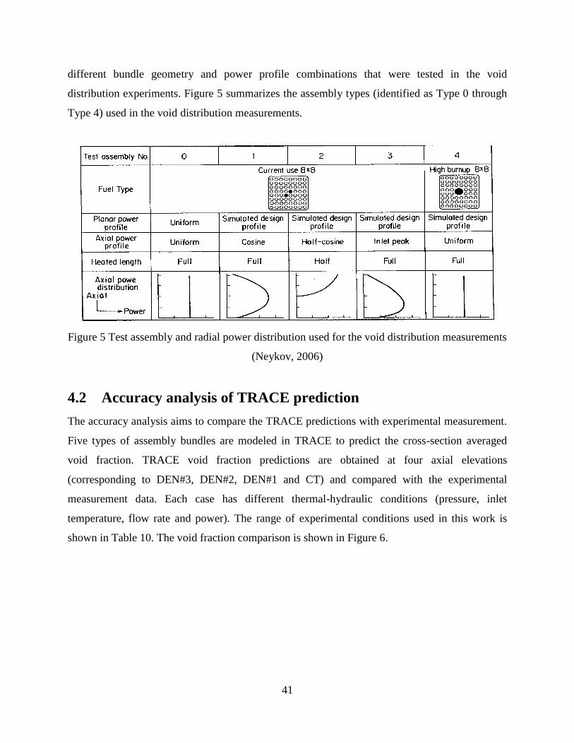
41

different bundle geometry and power profile combinations that were tested in the void

distribution experiments. Figure 5 summarizes the assembly types (identified as Type 0 through

Type 4) used in the void distribution measurements.

Figure 5 Test assembly and radial power distribution used for the void distribution measurements

(Neykov, 2006)

4.2 Accuracy analysis of TRACE prediction

The accuracy analysis aims to compare the TRACE predictions with experimental measurement.

Five types of assembly bundles are modeled in TRACE to predict the cross-section averaged

void fraction. TRACE void fraction predictions are obtained at four axial elevations

(corresponding to DEN#3, DEN#2, DEN#1 and CT) and compared with the experimental

measurement data. Each case has different thermal-hydraulic conditions (pressure, inlet

temperature, flow rate and power). The range of experimental conditions used in this work is

shown in Table 10. The void fraction comparison is shown in Figure 6.

42

Table 10 Variation of experimental conditions (Neykov, 2006)

Parameters Variations

Pressure (MPa) 3.9 - 8.7

Inlet temperature ( ∘C) 238 - 292

Inlet subcooling (kJ/kg) 50. - 56.

Flow rate ( t/h) 10. - 70.

Power (MW) 0.62 - 7.3

Exit quality (%) 8 - 25

Exit void fraction (%) 45 - 90

Figure 6 shows a comparison between the predicted and measured void fraction at four axial

elevations (DEN #3, DEN #2, DEN #1 and CT). Overall TRACE captures correct trend. In

general, TRACE predictions for the lowest and highest axial elevations (DEN #3 and CT) are

close to the measurement. However, TRACE predictions in the middle elevations (DEN #2 and

DEN #1) tend to under-estimate the void fraction, with an absolute difference of about 5-10%.

Both measurement and TRACE uncertainties contribute to the difference.

43

Figure 6 Comparison of TRACE and measurement void fraction

0 10 20 30 40 50 60 70 80 90 1000

10

20

30

40

50

60

70

80

90

100

Measured void fraction (%)

Pred

icte

d v

oid

fra

cti

on

(%

)

Void Fraction comparison for assembly: 0

CT

DEN.#1

DEN.#2

DEN.#3

0 10 20 30 40 50 60 70 80 90 1000

10

20

30

40

50

60

70

80

90

100

Measured void fraction (%)

Pred

icte

d v

oid

fra

cti

on

(%

)

Void Fraction comparison for assembly: 1

CT

DEN.#1

DEN.#2

DEN.#3

0 10 20 30 40 50 60 70 80 90 1000

10

20

30

40

50

60

70

80

90

100

Measured void fraction (%)

Pred

icte

d v

oid

fra

cti

on

(%

)

Void Fraction comparison for assembly: 2

CT

DEN.#1

DEN.#2

DEN.#3

0 10 20 30 40 50 60 70 80 90 1000

10

20

30

40

50

60

70

80

90

100

Measured void fraction (%)

Pred

icte

d v

oid

fra

cti

on

(%

)

Void Fraction comparison for assembly: 3

CT

DEN.#1

DEN.#2

DEN.#3

0 10 20 30 40 50 60 70 80 90 1000

10

20

30

40

50

60

70

80

90

100

Measured void fraction (%)

Pred

icte

d v

oid

fra

cti

on

(%

)

Void Fraction comparison for assembly: 4

CT

DEN.#1

DEN.#2

DEN.#3

0 10 20 30 40 50 60 70 80 90 100-20

-10

0

10

20

30

40

Measured void fraction (%)

Ab

solu

te e

rro

r o

f p

red

icti

on

TRACE void fraction prediction error

CT

DEN.#1

DEN.#2

DEN.#3

44

4.3 Sensitivity analysis of model parameters

Many parameters contribute to the uncertainties in TRACE prediction. The focus of this thesis is

the internal physical model parameters used in TRACE. TRACE (version 5.0 Patch 4) includes

options for uncertainty quantification by allowing the adjustment of 36 physical model

parameters from the input file. Following a sensitivity analysis of all 36 physical models, Table

11 (Hu, 2015) shows four parameters that are the most important (most sensitive) for void

fraction prediction. Sensitivity analysis shows that other physical model parameters, such as

liquid to interface bubbly-slug heat transfer coefficient and nucleate boiling heat transfer

coefficient, have little to no effect on void fraction prediction. These coefficients are not shown

in Table 11.

Table 11 Sensitivity coefficients † for Test assembly 4 at 4 axial locations (U.S. NRC, 2010)

Parameters DEN #3 DEN #2 DEN #1 CT

Single phase liquid to wall heat transfer -4.22 -0.36 -0.20 -0.03

Subcooled boiling heat transfer -10.77 -0.38 -0.20 -0.03

Wall drag -0.63 -1.28 -1.66 -2.97

Interfacial drag (bubbly/slug Rod

Bundle-Bestion)

0.73 1.94 2.25 0.93

†: Sensitivity coefficient = Δ𝑌

Δ𝑋

𝑋

𝑌∗ 100%

Table 11 shows an example of the calculated sensitivity coefficients. In the table, a

positive/negative sensitivity coefficient means that the predicted void fraction

increases/decreases with the parameters. From the sensitivity coefficient, we see that different

coefficients dominate at different locations. The sensitivity of single-phase liquid to wall heat

transfer coefficient decreases greatly at higher axial positions, because the single-phase liquid

exists primarily in the lower regions. Similarly, the subcooled boiling heat transfer is only

dominant in lower positions where subcooled boiling would occur. However, the drag force

tends to dominate in higher positions, thus the sensitivity is larger there. The sensitivity

coefficients are different for different thermal-hydraulic conditions and assembly geometry.

These four physical models are observed to be important for all BFBT cases. The sensitivity

coefficients are necessary for the sensitivity coefficient matrix (A) for MLE, MAP and MCMC

algorithm.

45

4.4 Validation of linearity assumption

Thus far, we have prepared necessary data for inverse uncertainty quantification by performing

accuracy analysis ( ��, ��0 ) and sensitivity analysis (A). However, the inverse uncertainty

quantification using MLE, MAP and MCMC relies on the linear assumption made in Eq. (42). It

is very important to validate this assumption prior to application.

Figure 7 Validation of linearity assumption for physical model parameters

Figure 7 shows the relation between the predicted void fraction and the four model parameters:

single-phase heat transfer coefficient, subcooled boiling heat transfer coefficient, wall drag

coefficient and interfacial drag (bubbly/slug Rod Bundle-Bestion) for one case. Figure 7(a)

shows that for void fraction prediction at the lowest axial position (DEN #3), the linearity

assumption is valid for a ±0.5 variation of model parameters. Figure 7(b) shows that for void

fraction prediction at the middle of heated section (DEN #2), the linearity assumption is valid for

a smaller variation of model parameters. The results are qualitatively similar for other axial

locations and other test cases. For this work, we use the model parameter variation of [-0.5, 0.5]

as the range where the linearity assumption is valid.

-0.5 -0.4 -0.3 -0.2 -0.1 0 0.1 0.2 0.3 0.4 0.5-4

-2

0

2

4

6

8

Relative change in model parameters

Ch

an

ge i

n v

oid

fra

cti

on

ou

tpu

t

Linearity relation in location DEN #3 assembly 4

Single phase heat transfer

Subcooled boiling heat transfer

Wall drag

Interfacial drag (bubbly/slug Rod Bundle-Bestion)

-0.5 -0.4 -0.3 -0.2 -0.1 0 0.1 0.2 0.3 0.4 0.5-2

-1.5

-1

-0.5

0

0.5

1

Relative change in model parameters

Ch

an

ge i

n v

oid

fra

cti

on

ou

tpu

t

Linearity relation in location DEN #2 assembly 4

Single phase heat transfer

Subcooled boiling heat transfer

Wall drag

Interfacial drag (bubbly/slug Rod Bundle-Bestion)

(a) (b)

46

4.5 Inverse uncertainty quantification with MLE, MAP and

MCMC

Before we can apply the MLE, MAP and MCMC algorithm, we also need information for the

random error of the experimental measurement. In this work, we assume the experimental error

is uniformly distributed on [-5, 5].

Many data sets could be used for the inverse uncertainty quantification algorithm. For the

purpose of this thesis, we use the data from Test assembly 4 axial location DEN #3. Two model

parameters, subcooled boiling heat transfer coefficient and interfacial drag (bubbly/slug Rod

Bundle-Bestion), are chosen as the �� random variables because they have the largest sensitivity

coefficients.

4.5.1 Criterion for selecting test cases

Some cases in the BFBT benchmark are invalid for inverse uncertainty quantification calculation,

and there are two main reasons why. One reason is that the measured void fraction is obviously

wrong, in some cases being less than 0 or larger than 1. The other reason is that the sensitivity

coefficient is too small, which makes the sensitivity coefficient matrix (A) close to singular.

Three criteria are implemented to select appropriate test cases:

1. The measured void fraction should be positive.

2. The predicted void fraction should be positive.

3. The absolute value of the sensitivity coefficient should be larger than a pre-set tolerance

(0.1 in this work).

4.5.2 Inverse uncertainty quantification results with MLE

We apply the MLE algorithm with the data obtained in the previous sections. The results are

listed in Table 12.

Table 12 Estimated distribution of two model parameters with MLE

Algorithms Subcooled boiling HTC Interfacial drag(bubbly/slug) Correlation

MLE 1a 1.15 ± 0.05 1.70 ± 0.15 N/A

MLE 1b 1.15 ± 0.05 1.70 ± 0.17 0.31

MLE 2 1.17 ± 1.36 1.76 ± 0.49 N/A

47

Three MLE algorithms give consistent results for the mean value of the model parameters, but

the algorithm MLE 2 gives a significantly higher variance. The mean value is a translation

parameter estimated by the maximization step and has little dependence on the variance

estimation. The algorithm MLE 2 gives a larger variance because of the independence

assumption between the output variables. Another observation is that the correlation calculated

by MLE 1b shows that these two model parameters are loosely and positively correlated.

4.5.3 Inverse uncertainty quantification results with MAP

The application of MAP algorithm requires that we provide the hyperparameters of the conjugate

prior distribution, which have to be estimated by some prior knowledge. The results from MLE

estimation is a good choice if the MAP algorithm is applied to different data. If the same data are

used, we should provide some prior knowledge.

Table 13 shows the assumption of the conjugate prior distribution. Because we do not have prior

information on the expectation value of prior �� and ��2, they are both assumed to be 1.0. A

mean value of 1.0 means the model parameters should not be adjusted. This is a critical

limitation for the application of MAP algorithm.

Table 13 Value of prior distribution hyperparameters used in MAP application

Variables Meaning Value

𝑟 shape factor of normal-inverse gamma distribution (3,3)T

�� shape factor of normal-inverse gamma distribution (1.0,1.0)T

𝛽 expectation value of prior �� (1.0,1.0)T

𝜆 expectation value of prior ��2 (1.0,1.0)T

The MAP results are shown in Table 14. We see that because of our prior information, the

estimated mean value of the two model parameters is closer to 1.0 compared with MLE

estimation . In addition, the estimated correlation is smaller, because the two model parameters

are independent in prior distribution. If different prior distribution is used, the estimation results

will change. For example, based on accuracy analysis in Section 4.2, we might be able to

qualitatively estimate what the prior distribution should be and then choose more appropriate

prior distribution.

48

Table 14 Estimated distribution of two model parameters with MAP

Algorithms Subcooled boiling HTC Interfacial drag(bubbly/slug) Correlation

MAP 1 1.06 ± 0.21 1.24 ± 0.46 0.16

MAP 2 1.08 ± 1.23 1.31 ± 0.49 N/A

4.5.4 Inverse uncertainty quantification results with MCMC

The application of MCMC algorithm requires a prior distribution. The prior distributions used in

this work for MCMC 1, 2, 3 are listed in Table 15.

Table 15 Prior distribution used in MCMC application

Algorithms Prior type Prior distribution

MCMC 1 Non-informative 1

(𝜎1)2(𝜎2)2

MCMC 2 Conjugate the same as Table 13

MCMC 3 Uniform �� ∈ [0.5,1.5] × [0.5,1.5], ��2 ∈ [0. ,1.0] × [0. ,1.0]

The results of MCMC estimation are listed in Table 16. The main observations are:

For MCMC 1, the estimation results are close to MLE estimation, which is expected

because we add little information than the MLE by adding the non-informative prior

distribution.

For MCMC 2, the estimation results are close to the MAP 1 estimation, because these

two algorithms use the same posterior distribution.

For MCMC 3, the estimation results are limited to a range where the linearity

assumption is valid. Test on MCMC 3 with a larger interval, for example �� ∈ [0. ,2.0] ×

[0. ,2.0], the estimation results becomes closer to MLE estimation, because we add less

limitation/information to the prior distribution.

Table 16 Estimated distribution of two model parameters with MCMC

Algorithms Subcooled boiling HTC Interfacial drag(bubbly/slug) Correlation

MCMC 1 1.15 ± 0.05 1.69 ± 0.21 N/A

MCMC 2 1.11 ± 0.29 1.46 ± 0.52 N/A

MCMC 3 1.11 ± 0.12 1.32 ± 0.50 N/A

49

4.6 Validation of MLE, MAP and MCMC results

In Section 4.5, we obtained physical model uncertainty estimates with different algorithms.

However, we do not know if these uncertainty estimates are valid. In this section, we are going to

validate these estimation results by performing forward uncertainty propagation using BFBT

benchmark data that was not used in Section 4.5 for the physical model uncertainty estimates. A

Monte Carlo sampling-based uncertainty propagation method is used: we sample the model

parameters according to their estimated distributions, perform TRACE calculations and process

the uncertainties of TRACE predictions.

There are 8 estimation results in Section 4.5, from which we selected two bounding results to

perform the forward uncertainty propagation calculation: results from MLE 1a (Table 12) and

MCMC 3 (Table 16).The physical model uncertainty estimates presented in Section 4.5 were

obtained with data obtained from axial location (DEN #3) of Test assembly 4. To validate the

results with forward uncertainty propagation, we are going to perform new TRACE calculations

for different axial locations.

4.6.1 Validation of MLE results with Test assembly 4

The forward uncertainty propagation process includes the following steps:

1. Monte Carlo sampling: the selected model parameters are sampled according to their

distribution.

2. TRACE input preparation: the model parameters are adjusted in TRACE input file based

on sampled values.

3. TRACE calculation: void fraction is predicted at different axial locations.

4. Uncertainty information: the uncertainty information is derived from TRACE predictions.

Figure 8 shows a schematic view of the forward uncertainty propagation process. This process

takes significant computational effort because thousands of TRACE calculations are required.

However, the computation time can be reduced by performing TRACE calculations

simultaneously.

50

Figure 8 Schematic view of the forward uncertainty propagation process (Hu, 2015)

Figure 9 Comparison of TRACE predictions without and with uncertainty information of model

parameters

0 5 10 15 20 25 30 35 40 45 500

5

10

15

20

25

30

35

40

45

50

Measured void fraction (%)

Pred

icte

d v

oid

fra

cti

on

(%

)

Assembly 4101: DEN #3

TRACE-MLE 1a

TRACE-nominal

0 10 20 30 40 50 60 70 800

10

20

30

40

50

60

70

80

Measured void fraction (%)

Pred

icte

d v

oid

fra

cti

on

(%

)

Assembly 4101: DEN #2

TRACE-MLE 1a

TRACE-nominal

0 10 20 30 40 50 60 70 800

10

20

30

40

50

60

70

80

Measured void fraction (%)

Pred

icte

d v

oid

fra

cti

on

(%

)

Assembly 4: DEN #1

TRACE-MLE 1a

TRACE-nominal

20 30 40 50 60 70 8020

30

40

50

60

70

80

Measured void fraction (%)

Pred

icte

d v

oid

fra

cti

on

(%

)

Assembly 4: CT

TRACE-MLE 1a

TRACE-nominal

(a) (b)

(c) (d)

51

Figure 9 shows the comparison of TRACE predictions without and with uncertainty information

of model parameters. Based on the comparison, we find:

DEN #3: The MLE estimation was performed using data from this position. The original

TRACE predictions (TRACE-nominal) do not include uncertain model parameters, as

TRACE underestimates the void fraction in some cases while overestimates the void

fraction in other cases. The MLE algorithm tries to minimize the global error by adjusting

the two model parameters. The new TRACE predictions (TRACE-MLE 1a) are closer to

the measured data, see Figure 9(a).

DEN #2, 1: Though MLE estimation does not use data in these two locations, the new

TRACE predictions (TRACE-MLE 1a) are better than the original TRACE predictions

(TRACE-nominal), see Figure 9(b), 9(c). It is possible to further improve the TRACE

predictions at location DEN #2, 1 by performing MLE estimation using data from these

locations.

CT: At this location, where the void fraction is considerably larger, the flow regime has

typically developed into annular or mist flow. The two selected models, subcooled

boiling heat transfer coefficient and interfacial drag (bubbly-slug), have little effect on

the void fraction at this location. The new TRACE predictions (TRACE-MLE 1a) are

essentially the same as the original predictions (TRACE-nominal), see Figure 9(d).

4.6.2 Validation of MLE result vs MCMC result

We validated the results from algorithm MCMC 3 the same way as MLE1a in Section 4.6.1.

Because the void fraction comparison is very similar to Figure 9, we compare the error

distribution between TRACE-nominal, TRACE-MLE1a and TRACE-MCMC3, the comparison

is shown in Figure 10.

52

Figure 10 Error distribution of TRACE calculation without and with uncertainty information in

model parameters

Figure 10 shows that the TRACE-MLE1a and TRACE-MCMC3 prediction error is distributed

more towards smaller error compared with TRACE predictions without uncertainty model

parameters (TRACE-nominal). However, comparison of MLE 1a and MCMC 3 shows that the

MLE 1a results are more accurate than MCMC 3 results. This is most likely due to using an

inaccurate prior distribution.

4.7 Summary of Chapter 4

In this Chapter, we applied the MLE, MAP and MCMC algorithms to BFBT benchmark data and

estimated the uncertainty distribution of two model parameters: subcooled boiling heat transfer

coefficient and interfacial drag (bubbly/slug rod bundle) coefficient.

These algorithms tend to give various estimation results. This is expected especially for MAP

and MCMC algorithms, because the assumption of the unknown prior distribution is difficult and

vary. Despite the differences in these algorithms, we find that the estimation results are

consistent. For example, if the prior distribution for MCMC algorithm is chosen to be uniform (1)

0 2 4 6 8 10 120

10

20

30

40

50

60

70

Absolute error

co

un

t

Error distribution: Assembly 4

TRACE-Nominal

TRACE-MCMC 3

TRACE-MLE 1a

53

on the entire domain, the MLE and MCMC algorithms are mathematically identical; this is what

we find from the comparison of MLE results with MCMC 1 and MCMC 3.

After obtaining the uncertainty estimates, we validated the uncertainty estimates by applying the

estimated distributions of model parameters to TRACE prediction. The new predictions succeed

in reducing the void fraction prediction error, but it is not possible to eliminate all prediction

error. We are only adjusting two model parameters, and there exists uncertainties in all model

parameters.

This work shows the difficulty of choosing a proper prior distribution for Bayesian-based MAP

and MCMC algorithms, which is the primary limitation of Bayesian-based methods. However, if

we could obtain accurate prior information, the MAP and MCMC algorithms would be more

powerful than MLE algorithm.

54

5 Discussion

There are several important features in the algorithms developed in this thesis. The first feature is

the potential to apply the algorithm to estimate many physical models simultaneously. The

algorithms developed in thesis are all generalized into matrix/vector form, which makes them

valid for any number of input physical parameters and outputs. For example, we can estimate the

uncertainties of three or more physical models at the same time provided with a consistent

sensitivity coefficient matrix and output data. We tested the algorithms with only two input

physical parameters because of the considerable computation load in calculating the sensitivity

coefficients using TRACE. In addition, the algorithms could be implemented in any

programming language very easily.

The second feature is that the MAP and MCMC algorithm considers prior information. Given the

prior information and new experiment data, the MAP and MCMC algorithms are capable of

updating our knowledge of the uncertainty in the models. The available prior information and

single experiment data might not be enough to give the correct uncertainty information. However,

this feature enables us update our knowledge whenever there is new experiment data.

The third feature is the capability of the MCMC algorithm in processing any form of prior

information and different models. Compared with the MLE and MAP algorithm, the MCMC

algorithm is capable of working with more general likelihood functions and prior distributions.

For example, we could avoid the linearity assumption with more advanced MCMC algorithm

and get a more accurate estimation. Future work on developing advanced MCMC algorithm

would be valuable.

The fourth feature is the wide application field of these algorithms. These algorithms do not

depend on any properties of experiment nor of modeling. Thus, the algorithms could be applied

to many other problems. For example, the algorithm could be applied to estimate the

uncertainties of cross section data used in a neutron transport problem.

55

6 Conclusion

Uncertainty information of physical model parameters is important for the purposes of

uncertainty quantification, such as best estimate plus uncertainty calculation. In this work, the

MLE, MAP and MCMC algorithms based on Bayesian analysis are developed, tested and

applied. Numerical tests with artificial data verified the implementation of these algorithms. The

application of these algorithms to BFBT benchmark data shows the typical work flow for

applying these algorithms. Also, the application to BFBT benchmark data validated these

algorithms.

We applied the MLE, MAP and MCMC algorithms to BFBT benchmark data and estimated the

uncertainty distribution of two model parameters: subcooled boiling heat transfer coefficient and

interfacial drag (bubbly/slug rod bundle) coefficient. These algorithms tend to give various

estimation results. This is expected especially for MAP and MCMC algorithms, because the

assumption of the unknown prior distribution is difficult and vary. Despite the differences in

these algorithms, we find that the estimation results are consistent.

After obtaining the uncertainty estimates, we validated the uncertainty estimates by applying the

estimated distributions of model parameters to TRACE prediction. The new predictions succeed

in reducing the void fraction prediction error, but it is not possible to eliminate all prediction

error. We are only adjusting two model parameters, and there exists uncertainties in all model

parameters. Application of the algorithms to other physical models and experimental data will be

helpful for future work.

56

7 Future Work

These algorithms are capable of reducing prediction error and provide uncertainty information

for further analysis. However, a few problems exist and needs future work.

Assumption: A lot of assumptions were made to derive the algorithms. Two main assumptions

are an assumed Gaussian distribution of output variables and an assumed linearity relation

between input model parameters and output variables. These assumptions are required to obtain

an analytical form of likelihood function. However, the statistical information of these variables

is not known. For a more general case, it might be not possible to get analytical form of

likelihood function. There is a way to process more general case by calculating and maximizing

the likelihood function numerically. The likelihood function could be calculated numerically

using Monte Carlo integration and could be maximized using Newton’s method. However, the

numerical calculation is much more expensive and has convergence issues.

Uncertain parameters: In practical application, such as with TRACE, many uncertain

parameters contribute to prediction error. In current algorithms, we are unable to account for

other uncertain parameters except for selected model parameters, which means the validity of

estimated results is not guaranteed.

Prior information: As evident, the prior information is critical in applying MAP and MCMC

algorithm. Unless we are confident with our prior information, it is not reliable to apply the MAP

and MCMC algorithm. An algorithm to initially estimate the prior information might be helpful,

but the algorithm would not work on the same data as MLE, MAP and MCMC.

Experimental data: The validity of experimental data determines the validity of estimated

results. For example, if obviously incorrect measurements exist, we would need to find and

remove these data before applying the algorithms. The process of removing data negates the

validity of estimation results. A standard algorithm in choosing data is necessary.

57

REFERENCES Boyack, B. (1990). Quantifying reactor safety margins part1: An overview of the code scaling,

applicability, and uncertainty evalulation methodology. Nuclear Engineering and Design.

Chib, S. (1995). Understanding the metropolis-hastings algorithm. The amerian statistican, 49(4),

327-335.

Gajev, I. (2014). Sensitivity analysis of input uncertain parameters on BWR stability using

TRACE/PARCS. Annals of Nuclear Energy, 67, 49-58.

Gelman, A. (2014). Bayesian data analysis. London: Chapman & Hall/CRC.

Gilks, W. R. (2005). Markov Chain monte carlo. John Wiley & Sons, Ltd.

Giunta, A. A. (2007). DAKOTA, a multilevel parallel object-oriented framework for design

optimization, parameter estimation, uncertainty quantification, and sensitivity analysis:

Version 4.1 reference manual. Albuquerque: NM: Sandia National Laboratories.

Hu, G. (2015). Uncertainty quantification of TRACE subcooled boiling model using BFBT

experiments. The 16th International Topical Meeting of Reactor Thermal Hydraulics

(NURETH-16). Chicago.

Ishii, M. (1977). One-dimensional drift-flux model and constitutive equations for relative motion

between phases in various two-phase flow regimes. Chicago: Argonne National Lab.

Ishii, M. (2010). Thermo-fluid dynamics of two-phase flow. Springer Science & Bussiness

Media.

Jaynes, E. T. (2003). Probability theory: the logic of science. Cambridge university press.

Kaichiro, M. (1984). Flow regime transitation criteria for upward two-phase flow in vertical

tubes. International Journal of Heat and Mass Transfer, 27(5), 723-737.

Kennedy, M. C. (2001). Bayesian calibration of computer models. Journal of the Roya Statistical

Society, Series B, 424-462.

Lee, S. H. (2009). A comparative study of uncertainty propagation methods for black-box-type

problems. Structural and Multidisciplinary Optimization, 116, 239-253.

Malachlan, G. (2007). The EM algorithms and extensions. John Wiley & Sons.

Mooney, C. Z. (1997). Monte Carlo simulation. Sage Publication.

Neykov, B. (2006). NUPEC BWR Full-size Fine-mesh Bundle Test (BFBT) Benchmark. OECD

Papers 6.7.

Scholz, F. W. (1985). Maximum likelihood estimation. Encyclopedia of Statistical Sciences.

Shrestha, R. (2015). Inverse uncertainty quantification of input model parameters for

thermal-hydraulics simulations using expectation-maximization under Bayesian

framework. Journal of Applied Statistics, 1-16.

U.S. NRC. (1989). Best-estimate calculation of emergency core cooling system performance.

U.S. Nuclera Regulartory Commission, Office of Nuclear Regulatory Research.

U.S. NRC. (2001). RELAP5/MOD3.3 code manual Vols. 1-8. Rockvile: Idaho Falls, ID:

Information Systems Laboratories.

U.S. NRC. (2010). TRACE V5.0 Theory Mannual-Field Equations, Solution Methods and

Physical Models. U.S. Nuclear Regulatory Commission.

Zuber, N. (1965). Average volumetric concentration in two-phase flow systems. Journal of Heat

Transfer, 87(4), 453-468.