F A C U L T Y O F S C I E N C E U N I V E R S I T Y O F C O P E N H A G E N

Inversion of Block Tridiagonal Matrices Egil Kristoffer Gorm Hansen & Rasmus Koefoed Jakobsen Department of Computer Science – January 14th, 2010

Supervisor: Stig Skelboe

Abstract

We have implemented a prototype of the parallel block tridiagonal matrix inver-sion algorithm presented by Stig Skelboe [Ske09] using C# and the Microsoft.NETplatform. The performance of our implementation was measured using the Monoruntime on a dual Intel Xeon E5310 (a total of eight cores) running Linux. Wi-thin the context of the software and hardware platform, we feel our results supportSkelboes theories. We achieved speedups of 7.348 for inversion of block tridiago-nal matrices, 7.734 for LU-factorization, 7.772 for minus – matrix – inverse-matrixmultiply (−A · B−1), and 7.742 for inversion of matrices.

Resumé

Vi har implementeret en prototype i C# og Microsoft.NET af den parallellealgoritme til invertering af blok-tridiagonale matricer præsenteret af Stig Skelboe[Ske09]. Vi har foretaget ydelsesmålinger af vores prototype ved hjælp af Mono påen dual Intel Xeon E5310 (i alt otte kerner), der kører Linux. Vi mener at haveunderstøttet Skelboes teorier, indenfor rammerne af platformen. Vores resultaterinkluderer speedups på optil 7,348 for invertering af blok-tridiagonale matricer, 7,734for LU-faktorisering, 7,772 for minus – matrix – invers-matrix multiplikation (−A ·B−1), and 7,742 for invertering matricer.

2

ContentsList of Figures 5

List of Listings 6

List of Tables 7

1 Introduction 8

2 Theory and description of the algorithms 92.1 Theory . . . . . . . . . . . . . . . . . . . . . . . . . . . . . . . . . . . . . . 92.2 Tiling . . . . . . . . . . . . . . . . . . . . . . . . . . . . . . . . . . . . . . 102.3 The matrix operations . . . . . . . . . . . . . . . . . . . . . . . . . . . . . 10

2.3.1 LU-factorization . . . . . . . . . . . . . . . . . . . . . . . . . . . . . 112.3.2 Minus – matrix – inverse-matrix multiply . . . . . . . . . . . . . . . 132.3.3 Matrix Inverse . . . . . . . . . . . . . . . . . . . . . . . . . . . . . . 14

2.4 Utilizing the combined operations in block tridiagonal matrix inversion . . 16

3 Implementation 183.1 Workflow . . . . . . . . . . . . . . . . . . . . . . . . . . . . . . . . . . . . 183.2 Overall design . . . . . . . . . . . . . . . . . . . . . . . . . . . . . . . . . . 203.3 Components . . . . . . . . . . . . . . . . . . . . . . . . . . . . . . . . . . . 20

3.3.1 Manager (and workers) . . . . . . . . . . . . . . . . . . . . . . . . . 203.3.2 IProducer<T> . . . . . . . . . . . . . . . . . . . . . . . . . . . . . . 223.3.3 The matrix operation producer pattern . . . . . . . . . . . . . . . . 233.3.4 The straightforward producers . . . . . . . . . . . . . . . . . . . . . 233.3.5 The LUFactorization producer . . . . . . . . . . . . . . . . . . . . . 243.3.6 The MinusMatrixInverseMatrixMultiply producer . . . . . . . . . . 263.3.7 The Inverse producer . . . . . . . . . . . . . . . . . . . . . . . . . . 273.3.8 The BlockTridiagonalMatrixInverse producer . . . . . . . . . . . . . 273.3.9 Possible improvements and issues . . . . . . . . . . . . . . . . . . . 28

4 Performance measurements 314.1 Experiment setup . . . . . . . . . . . . . . . . . . . . . . . . . . . . . . . . 314.2 Experiment results and analysis . . . . . . . . . . . . . . . . . . . . . . . . 34

4.2.1 Presentation and analysis of LU-factorization . . . . . . . . . . . . 354.2.2 Presentation and analysis of Inverse and Minus – Matrix – Inverse-

Matrix Multiply . . . . . . . . . . . . . . . . . . . . . . . . . . . . . 374.2.3 Presentation and analysis of Multiply, Plus Multiply, Minus Plus Plus 394.2.4 Presentation and analysis of Block Tridiagonal Matrix Inversion . . 40

4.3 Possible improvements . . . . . . . . . . . . . . . . . . . . . . . . . . . . . 424.4 What could have been . . . . . . . . . . . . . . . . . . . . . . . . . . . . . 43

3

5 Conclusion 44

References 45

A Measurement results 46BTM 10x750x750 - collected statistics . . . . . . . . . . . . . . . . . . . . . . . 48BTM 10x750x750 - calculated statistics . . . . . . . . . . . . . . . . . . . . . . . 49BTM 10x750x750 - measurement including extra statistics - collected statistics

part 1 . . . . . . . . . . . . . . . . . . . . . . . . . . . . . . . . . . . . . . 50BTM 10x750x750 - measurement including extra statistics - collected statistics

part 2 . . . . . . . . . . . . . . . . . . . . . . . . . . . . . . . . . . . . . . 51BTM 10x750x750 - measurement including extra statistics - calculated statistics 52BTM 10x500x500 - collected statistics . . . . . . . . . . . . . . . . . . . . . . . 53BTM 10x500x500 - calculated statistics . . . . . . . . . . . . . . . . . . . . . . . 54BTM 100x100x200 - measurement including extra statistics - collected statistics 55BTM 100x100x200 - measurement including extra statistics - calculated statistics 56BTM 100x100x200 - collected and calculated statistics . . . . . . . . . . . . . . 57BTM 100x50x100 - collected and calculated statistics . . . . . . . . . . . . . . . 58BTM 100x150x250 - collected and calculated statistics . . . . . . . . . . . . . . 59BTM 200x100x200 - collected and calculated statistics . . . . . . . . . . . . . . 60BTM 50x100x200 - collected and calculated statistics . . . . . . . . . . . . . . . 61LU-factorization: 3000x3000 - collected and calculated statistics . . . . . . . . . 62Inverse: 2500x2500 - collected and calculated statistics . . . . . . . . . . . . . . 63Minus – Matrix – Inverse-Matrix Multiply: 2500x2500 - collected and calculated

statistics . . . . . . . . . . . . . . . . . . . . . . . . . . . . . . . . . . . . . 64MinusPlusPlus: 5000x5000 - collected and calculated statistics . . . . . . . . . . 65Multiply: 2500x2500 - collected and calculated statistics . . . . . . . . . . . . . 66PlusMultiply: 2500x2500 - collected and calculated statistics . . . . . . . . . . . 67

4

List of Figures1 A sketch of how the quadratic block tridiagonal matrix, A, could look. . . 92 The tiling of a block aij . . . . . . . . . . . . . . . . . . . . . . . . . . . . 113 Tiled LU-factorization . . . . . . . . . . . . . . . . . . . . . . . . . . . . . 124 This illustrates how the psuedocode in figure 3 on page 12 runs . . . . . . 135 The modified psuedocode for tiled minus – matrix – inverse-matrix multiply 146 PIM algorithm for row i of c = bl−1 . . . . . . . . . . . . . . . . . . . . . . 157 Tiled matrix inversion from [Ske09], figure 9. Note that i and j are inter-

changed to improve readability. . . . . . . . . . . . . . . . . . . . . . . . . 158 The second iteration of calculating column 3 of the first step of Inverse . . 169 The scheduling of column 1 of the first step of the tiled matrix inverse . . . 1710 The scheduling of the first column of the second step of the tiled matrix

inverse . . . . . . . . . . . . . . . . . . . . . . . . . . . . . . . . . . . . . . 1711 Conceptual workflow of the parallel computations. . . . . . . . . . . . . . . 1912 Manager class diagram . . . . . . . . . . . . . . . . . . . . . . . . . . . . . 2013 Workflow of the GetWork method. . . . . . . . . . . . . . . . . . . . . . . . 2114 A generic interface called IProducer<T> . . . . . . . . . . . . . . . . . . . 2215 The workflow of the Find method in the OperationEnumerator class . . . . 2416 Template for the parallel operation pattern . . . . . . . . . . . . . . . . . . 2617 Speedup chart for parallel LU-factorization . . . . . . . . . . . . . . . . . . 3618 Speedup chart for parallel Inverse . . . . . . . . . . . . . . . . . . . . . . . 3719 Speedup chart for parallel Minus – Matrix – Inverse-Matrix Multiply . . . 3920 Speedup chart for parallel Block Tridiagonal Matrix Inversion . . . . . . . 41

5

Listings1 The implementation of the modified PDS algorithm . . . . . . . . . . . . . 252 This listing shows the implementation of the minus – matrix – inverse-matrix

multiply scheduling algorithm. . . . . . . . . . . . . . . . . . . . . . . . . . 293 This listing shows the implementation of the block matrix inverse scheduling

algortihm. . . . . . . . . . . . . . . . . . . . . . . . . . . . . . . . . . . . . 30

6

List of Tables1 Overview of experiments and matrix sizes used. . . . . . . . . . . . . . . . 322 Overview of best achieved speedups . . . . . . . . . . . . . . . . . . . . . . 343 Single threaded to single threaded tiled speedups . . . . . . . . . . . . . . 354 Speedup table for parallel LU-factorization . . . . . . . . . . . . . . . . . . 355 Speedup table for parallel Inverse . . . . . . . . . . . . . . . . . . . . . . . 386 Speedup table for parallel Minus – Matrix – Inverse-Matrix Multiply . . . 387 Summary of best speedups attained with eight threads in the different ex-

periments conducted. . . . . . . . . . . . . . . . . . . . . . . . . . . . . . . 408 Overview of best achieved speedups . . . . . . . . . . . . . . . . . . . . . . 449 BTM 10x750x750 - collected statistics . . . . . . . . . . . . . . . . . . . . . 4810 BTM 10x750x750 - calculated statistics . . . . . . . . . . . . . . . . . . . . 4911 BTM 10x750x750 - measurement including extra statistics - collected sta-

tistics part 1 . . . . . . . . . . . . . . . . . . . . . . . . . . . . . . . . . . . 5012 BTM 10x750x750 - measurement including extra statistics - collected sta-

tistics part 2 . . . . . . . . . . . . . . . . . . . . . . . . . . . . . . . . . . . 5113 BTM 10x750x750 - measurement including extra statistics - calculated sta-

tistics . . . . . . . . . . . . . . . . . . . . . . . . . . . . . . . . . . . . . . 5214 BTM 10x500x500 - collected statistics . . . . . . . . . . . . . . . . . . . . . 5315 BTM 10x500x500 - calculated statistics . . . . . . . . . . . . . . . . . . . . 5416 BTM 100x100x200 - measurement including extra statistics - collected sta-

tistics. . . . . . . . . . . . . . . . . . . . . . . . . . . . . . . . . . . . . . . 5517 BTM 100x100x200 - measurement including extra statistics - calculated sta-

tistics . . . . . . . . . . . . . . . . . . . . . . . . . . . . . . . . . . . . . . 5618 BTM 100x100x200 - collected and calculated statistics . . . . . . . . . . . 5719 BTM 100x50x100 - collected and calculated statistics . . . . . . . . . . . . 5820 BTM 100x150x250 - collected and calculated statistics . . . . . . . . . . . 5921 BTM 200x100x200 - collected and calculated statistics . . . . . . . . . . . 6022 BTM 50x100x200 - collected and calculated statistics . . . . . . . . . . . . 6123 LU-factorization: 3000x3000 - collected and calculated statistics . . . . . . 6224 Inverse: 2500x2500 - collected and calculated statistics . . . . . . . . . . . 6325 Minus – Matrix – Inverse-Matrix Multiply: 2500x2500 - collected and cal-

culated statistics . . . . . . . . . . . . . . . . . . . . . . . . . . . . . . . . 6426 MinusPlusPlus: 5000x5000 - collected and calculated statistics . . . . . . . 6527 Multiply: 2500x2500 - collected and calculated statistics . . . . . . . . . . 6628 PlusMultiply: 2500x2500 - collected and calculated statistics . . . . . . . . 67

7

1 IntroductionPerforming calculations in parallel is of increasing importance due to the stagnation inprocessor speed and increase in the number of processors and cores in computers. In thearticle [Ske09], Stig Skelboe presents a theoretical solution to the parallelization of inversionof a block tridiagonal matrix.

In this report we have documented our efforts to test Skelboes theories in practicethrough a prototype framework developed in C# on the Microsoft.NET platform. Theexperiments were performed on an eight core machine running Linux using the Monoruntime.

While we do reiterate key parts of Skelboes article related to our work, it may bebeneficial for the reader to have copy at hand. A general knowledge of object orienteddesign and the challenges of parallel programming is also suggested.

All the source code, full set of measurement results, and the source material for this re-port are available online at http://github.com/egil/Inversion-of-Block-Tridiagonal-Matricesor on the accompanying compact disc.

8

2 Theory and description of the algorithmsIn this section we will take a closer look at the theory and algorithms presented in [Ske09],and the modifications and derivations we have made. We do not recount [Ske09] in itsentirety. The content of this section is the basis for the implementation presented insection 3 on page 18.

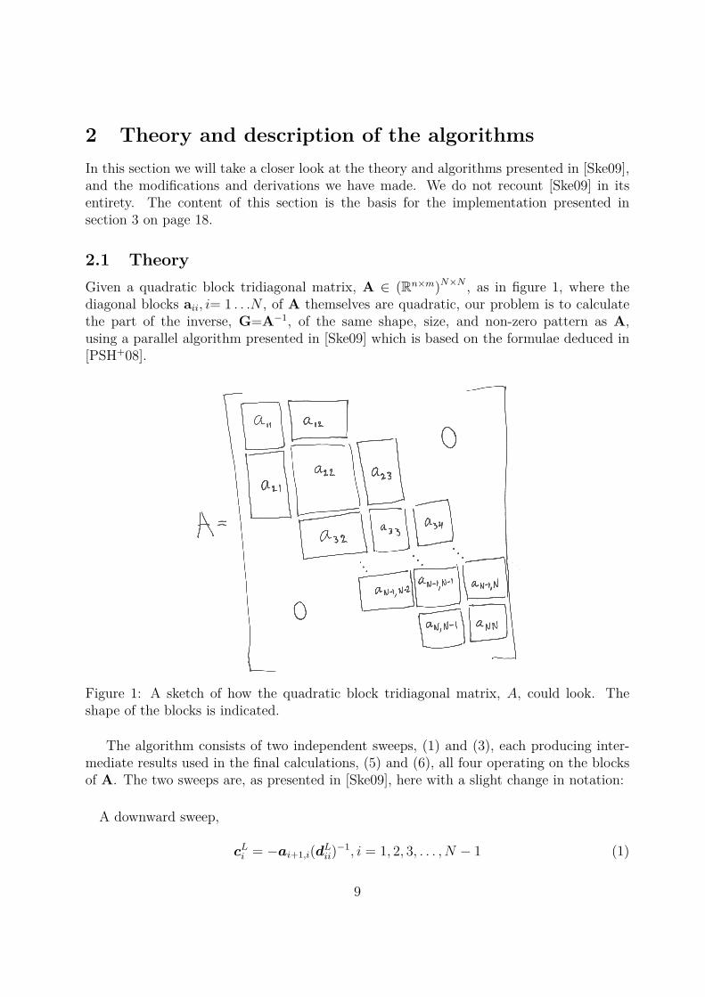
2.1 TheoryGiven a quadratic block tridiagonal matrix, A ∈ (Rn×m)N×N , as in figure 1, where thediagonal blocks aii, i= 1 . . .N , of A themselves are quadratic, our problem is to calculatethe part of the inverse, G=A−1, of the same shape, size, and non-zero pattern as A,using a parallel algorithm presented in [Ske09] which is based on the formulae deduced in[PSH+08].

Figure 1: A sketch of how the quadratic block tridiagonal matrix, A, could look. Theshape of the blocks is indicated.

The algorithm consists of two independent sweeps, (1) and (3), each producing inter-mediate results used in the final calculations, (5) and (6), all four operating on the blocksof A. The two sweeps are, as presented in [Ske09], here with a slight change in notation:

A downward sweep,

cLi = −ai+1,i(dLii)−1, i = 1, 2, 3, . . . , N − 1 (1)

9

where dL11 = a11

dLii = aii + cLi−1ai−1,i (2)An upward sweep,

cRi = −ai−1,i(dRii)−1, i = N,N − 1, N − 2, . . . , 2 (3)

where dRNN = aNN

dRii = aii + cRi+1ai+1,i (4)The final calculations for the blocks gij of G = A−1 are,

gii = (−aii + dLii + dRii)−1, i = 1, 2, 3, . . . , N (5)

gij = gii · cRi+1 · cRi+2 · · · cRj for i < j (6)gij = gii · cLi−1 · cLi−2 · · · cLj for i > j

2.2 TilingThe formulae presented in section 2.1 on the previous page work on a per block basis. Inorder to distribute the work over several processors, each block, aij, of A, is divided intoa number of tiles akl, making aij a block matrix on its own.

Figure 2 on the following page illustrates how a block aij is tiled into a block matrix.Note that the rightmost and bottom tiles may not be quadratic due to the tile size n notdividing the size of the block O and P .

It is important to use the same tile size, n, and tiling strategy on all blocks in order forthe tiled matrix operations to be meaningful.

Failing to do this, the formulae will be rendered incorrect at best, because numbers inthe wrong positions in the original matrix will be operated on. Most likely though, thetiled matrix operations will fail on account of tiles not matching size requirements whenfor example multiplying or adding two tiles together.

2.3 The matrix operationsIn this section we will look at some of the algorithms used in our calculations of theformulae presented in section 2.1 on the previous page.

We have modified the tiled matrix – inverse-matrix multiply algorithm from [Ske09]section 4 to incorporate the minus operation, which is always used in calculation of formulae(1) and (3), resulting in a tiled minus – matrix – inverse-matrix multiply algorithm.

When calculating formula (1), we first LU-factorize the term dLii before applying thetiled minus – matrix – inverse-matrix multiply algorithm.

Also, when calculating formula (2), we use a combined tiled addition and tiled matrixmultiplication named tiled plus – multiply when computing dLii .

10

Figure 2: The tiling of a block aij of size O×P into a block matrix of size N×M whereN= dO/ne ,M= dP/ne, and n is the chosen tile size. The tiles akl, k<N, j<M are of sizen×n. Unless n divides bothN andM , the rightmost tiles, akM are of size n×(P−

⌊Pn

⌋), and

the bottom tiles aNl are of size (O−⌊On

⌋)×n, making aNM of size (O−

⌊On

⌋)× (P−

⌊Pn

⌋).

The same tiled matrix operations are used in (3) and (4).In the calculations of the diagonal elements, gii, in (5), −aii+dLii+dRii is combined into

one tiled minus – plus – plus operation, LU-factorized and then inverted.The last formula (6) is a series of tiled matrix-matrix multiplications.Plus – multiply, minus – plus – plus, and matrix multiplication are all delightfully

parallel; there are no dependencies among the tiles, and we will not go into much detailwith these.

2.3.1 LU-factorization

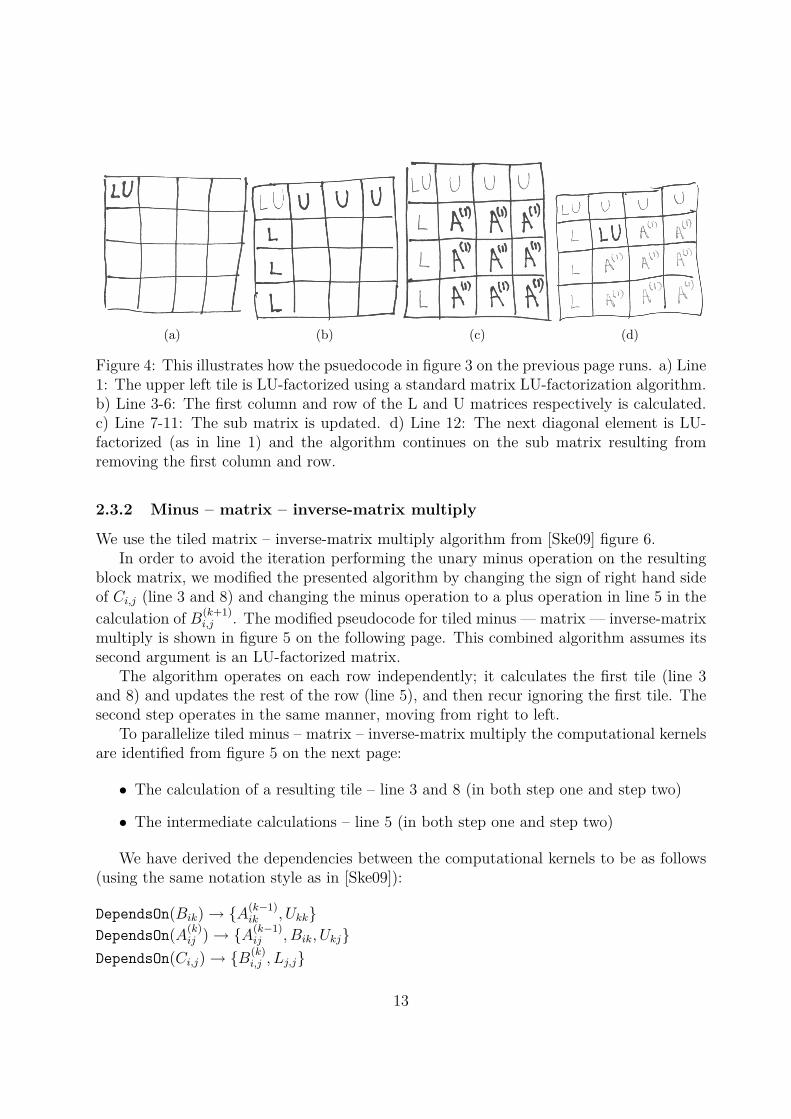
The psuedocode in figure 3 on the following page is from [Ske09]. Figure 4 on page 13illustrates how tiled LU-factorization is carried out.

To parallelize the algorithm in figure 3, the computational kernels are identified asfollows:

11

1 L11U11 = A(0)11

2 for k = 1 : (N − 1)3 for i = (k + 1) : N4 Lik = A(k−1)

ik U−1kk

5 Uki = L−1kkA

(k−1)ki

6 end7 for i = (k + 1) : N8 for j = (k + 1) : N9 A

(k)ij = A(k−1)

ij − LikUkj10 end11 end12 Lk+1,k+1Uk+1,k+1 = A(k)

k+1,k+113 end

Figure 3: Tiled LU-factorization

• Line 1 and 12 is an LU-factorization

• In line 4 there is an matrix inverse-matrix multiply

• In line 5 there is an inverse-triangular-matrix – matrix multiply

• Line 9 has a matrix – matrix multiply add

The dependencies, which are visible from the pseudocode, are summarized in the fol-lowing DependsOn function, reproduced from [Ske09] section 3.2.2. An operation is neverstarted before its dependencies are satisfied.

DependsOn(LiiUii)→ {A(i−1)ii }

DependsOn(A(k)ij )→ {A(k−1)

ij , Lik, Ukj}DependsOn(Lij)→ {A(j−1)

ij , Ujj}DependsOn(Uij)→ {Lii, A(i−1)

ij }

A scheduling of the operations is presented in [Ske09] section 3.2.2, basically interleavingthe for loops of the algorithm to continually free many dependencies1. The naive way toschedule the computational kernels results in periods where only one operation is runnable.To eliminate this when utilizing more cores, we will use the modified pipelined diagonalsweep elimination algorithm exemplified in [Ske09], figure 4.

1Finding the optimal scheduling is an NP-complete problem, so we will limit ourselves to the schedulesuggested in [Ske09].

12

(a) (b) (c) (d)

Figure 4: This illustrates how the psuedocode in figure 3 on the previous page runs. a) Line1: The upper left tile is LU-factorized using a standard matrix LU-factorization algorithm.b) Line 3-6: The first column and row of the L and U matrices respectively is calculated.c) Line 7-11: The sub matrix is updated. d) Line 12: The next diagonal element is LU-factorized (as in line 1) and the algorithm continues on the sub matrix resulting fromremoving the first column and row.

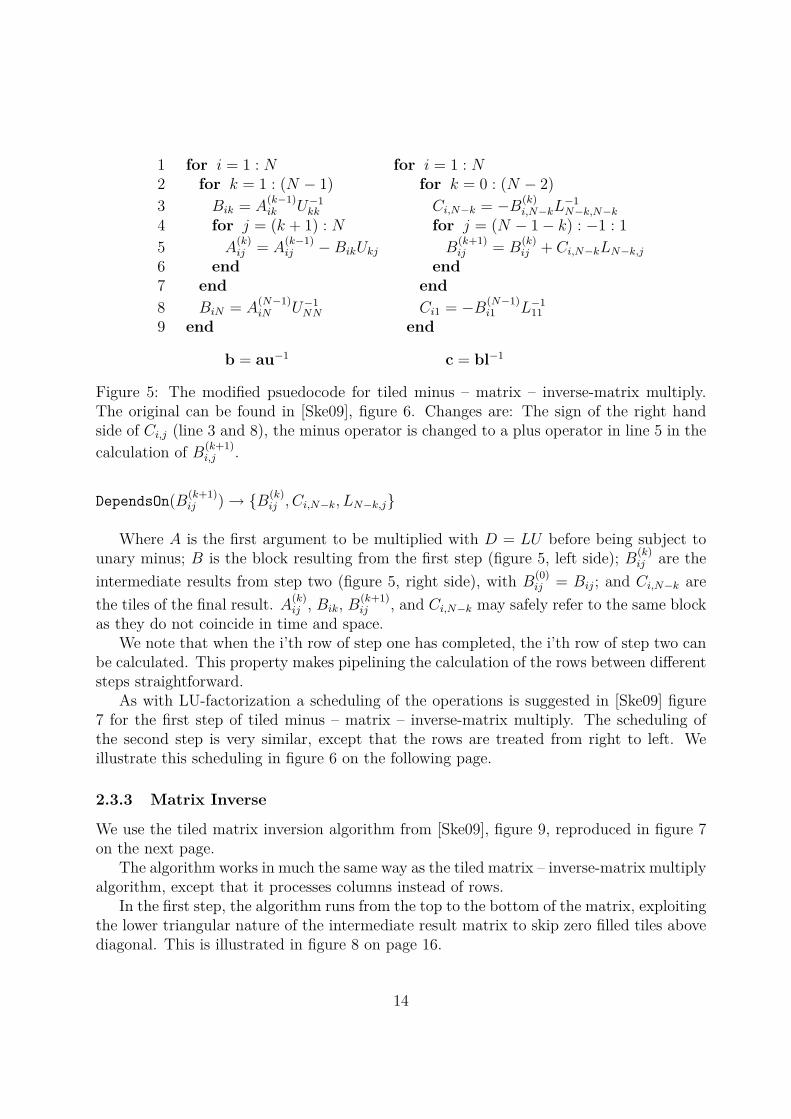
2.3.2 Minus – matrix – inverse-matrix multiply

We use the tiled matrix – inverse-matrix multiply algorithm from [Ske09] figure 6.In order to avoid the iteration performing the unary minus operation on the resulting

block matrix, we modified the presented algorithm by changing the sign of right hand sideof Ci,j (line 3 and 8) and changing the minus operation to a plus operation in line 5 in thecalculation of B(k+1)

i,j . The modified pseudocode for tiled minus — matrix — inverse-matrixmultiply is shown in figure 5 on the following page. This combined algorithm assumes itssecond argument is an LU-factorized matrix.

The algorithm operates on each row independently; it calculates the first tile (line 3and 8) and updates the rest of the row (line 5), and then recur ignoring the first tile. Thesecond step operates in the same manner, moving from right to left.

To parallelize tiled minus – matrix – inverse-matrix multiply the computational kernelsare identified from figure 5 on the next page:

• The calculation of a resulting tile – line 3 and 8 (in both step one and step two)

• The intermediate calculations – line 5 (in both step one and step two)

We have derived the dependencies between the computational kernels to be as follows(using the same notation style as in [Ske09]):

DependsOn(Bik)→ {A(k−1)ik , Ukk}

DependsOn(A(k)ij )→ {A(k−1)

ij , Bik, Ukj}DependsOn(Ci,j)→ {B(k)

i,j , Lj,j}

13

1 for i = 1 : N for i = 1 : N2 for k = 1 : (N − 1) for k = 0 : (N − 2)3 Bik = A(k−1)

ik U−1kk Ci,N−k = −B(k)

i,N−kL−1N−k,N−k

4 for j = (k + 1) : N for j = (N − 1− k) : −1 : 15 A

(k)ij = A(k−1)

ij −BikUkj B(k+1)ij = B(k)

ij + Ci,N−kLN−k,j6 end end7 end end8 BiN = A(N−1)

iN U−1NN Ci1 = −B(N−1)

i1 L−111

9 end end

b = au−1 c = bl−1

Figure 5: The modified psuedocode for tiled minus – matrix – inverse-matrix multiply.The original can be found in [Ske09], figure 6. Changes are: The sign of the right handside of Ci,j (line 3 and 8), the minus operator is changed to a plus operator in line 5 in thecalculation of B(k+1)

i,j .

DependsOn(B(k+1)ij )→ {B(k)

ij , Ci,N−k, LN−k,j}

Where A is the first argument to be multiplied with D = LU before being subject tounary minus; B is the block resulting from the first step (figure 5, left side); B(k)

ij are theintermediate results from step two (figure 5, right side), with B(0)

ij = Bij; and Ci,N−k arethe tiles of the final result. A(k)

ij , Bik, B(k+1)ij , and Ci,N−k may safely refer to the same block

as they do not coincide in time and space.We note that when the i’th row of step one has completed, the i’th row of step two can

be calculated. This property makes pipelining the calculation of the rows between differentsteps straightforward.

As with LU-factorization a scheduling of the operations is suggested in [Ske09] figure7 for the first step of tiled minus – matrix – inverse-matrix multiply. The scheduling ofthe second step is very similar, except that the rows are treated from right to left. Weillustrate this scheduling in figure 6 on the following page.

2.3.3 Matrix Inverse

We use the tiled matrix inversion algorithm from [Ske09], figure 9, reproduced in figure 7on the next page.

The algorithm works in much the same way as the tiled matrix – inverse-matrix multiplyalgorithm, except that it processes columns instead of rows.

In the first step, the algorithm runs from the top to the bottom of the matrix, exploitingthe lower triangular nature of the intermediate result matrix to skip zero filled tiles abovediagonal. This is illustrated in figure 8 on page 16.

14

1: Ci52: B

(1)i4

3: B(1)i3 Ci4

4: B(1)i2 B

(2)i3

5: B(1)i1 B

(2)i2 Ci3

6: B(2)i1 B

(3)i2

7: B(3)i1 Ci2

8: B(4)i1

9: Ci1

Figure 6: The scheduling of row i of the second step of the tiled minus - matrix - inverse-matrix multiply algorithm, using the same notation as [Ske09] figure 7. In this examplethe block matrix has 5 columns. The figure is read line by line.

1 for j = 1 : N for j = 1 : N2 for k = 0 : (N − j − 1) for k = 0 : (N − 2)3 Fk+j,j = L−1

k+j,k+jR(k)k+j,j GN−k,j = U−1

N−k,N−kF(k)N−k,j

4 for i = (j + k + 1) : N for i = (N − 1− k) : −1 : 15 R

(k+1)ij = R(k)

ij − Li,k+jFk+j,j F(k+1)ij = F (k)

ij − Ui,N−kGN−k,j6 end end7 end end8 FNj = L−1

NNR(N−j)Nj G1j = U−1

11 F(N−1)1j

9 end end

f = l−1r g = u−1f

Figure 7: Tiled matrix inversion from [Ske09], figure 9. Note that i and j are interchangedto improve readability.

In the second step, the algorithm runs from the bottom all the way to the top of thematrix.

To parallelize the tiled matrix inverse algorithm, the computational kernels are identi-fied as seen in figure 7:

• The calculation of a resulting tile – line 3 and 8 (in both step one and step two)

• The intermediate calculations – line 5 (in both step one and step two)

We have derived the dependencies between the computational kernels to be as follows:

15

Figure 8: The second iteration of calculating column 3 of the first step of Inverse. Thetiles above the diagonal are skipped. The example is of size 5× 5

DependsOn(Fk+j,j)→ {L−1k+j,k+j, R

(k)k+j,j}

DependsOn(R(k+1)ij )→ {R(k)

ij , Li,k+j, Fk+j,j}DependsOn(Gi,j)→ {U−1

i,i , F(k)i,j }

DependsOn(F (k+1)ij )→ {F (k)

ij , Ui,N−k, GN−k,j}

Fk+j,j, R(k+1)ij , GN−k,j, and F (k+1)

ij do not refer to the same tiles at the same time, andcan hence safely refer to same block matrix.

Similar to the pipelined properties of the parallel tiled matrix – inverse-matrix multiplyalgorithm, when the i’th column of step one is complete, the i’th column of step two canproceed.

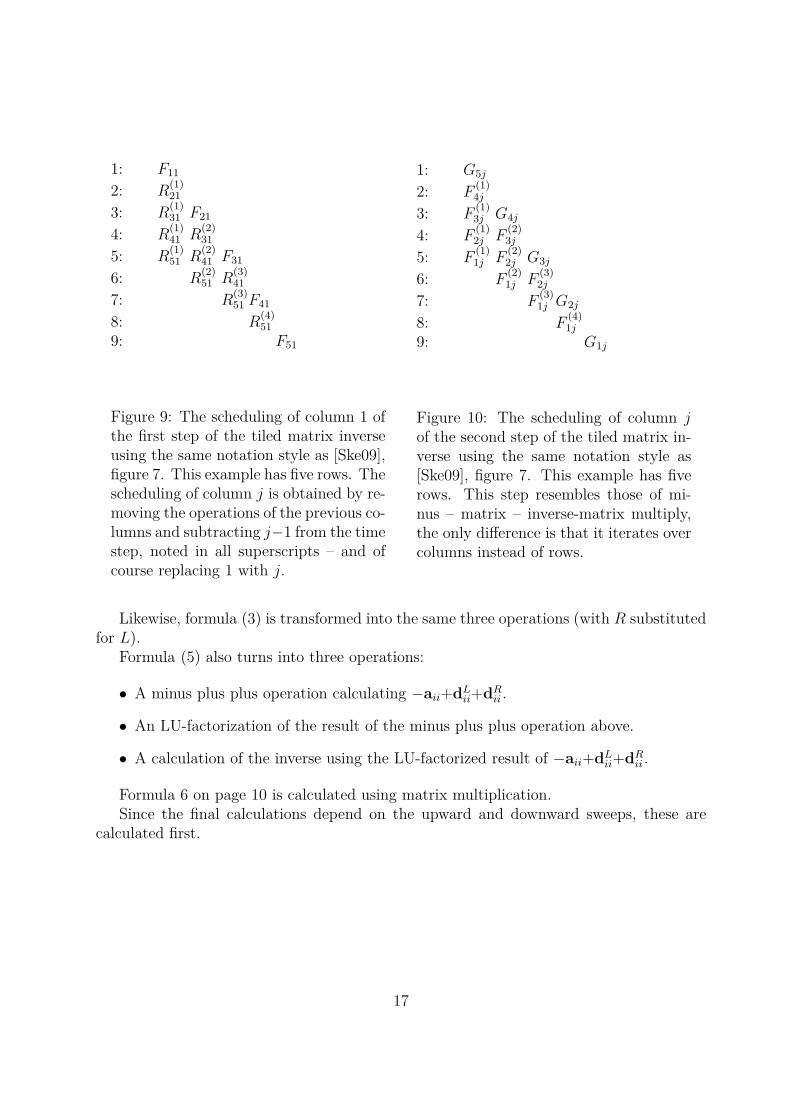
As suggested in [Ske09] section 5, we have derived a schedule similar to that of the tiledmatrix – inverse-matrix multiply algorithm. See figure 9 and 10 on the following page foran illustration of the schedule of step one and two respectively.

2.4 Utilizing the combined operations in block tridiagonal ma-trix inversion

When putting it all together, formula (1) becomes three operations:

• A plus multiply operation is used to calculate dLii from (2)

• An LU-factorization of dLii from (1)

• A minus – matrix – inverse-matrix multiply operation calculating cLi−1 from (1)

16

1: F11

2: R(1)21

3: R(1)31 F21

4: R(1)41 R

(2)31

5: R(1)51 R

(2)41 F31

6: R(2)51 R

(3)41

7: R(3)51 F41

8: R(4)51

9: F51

Figure 9: The scheduling of column 1 ofthe first step of the tiled matrix inverseusing the same notation style as [Ske09],figure 7. This example has five rows. Thescheduling of column j is obtained by re-moving the operations of the previous co-lumns and subtracting j−1 from the timestep, noted in all superscripts – and ofcourse replacing 1 with j.

1: G5j

2: F(1)4j

3: F(1)3j G4j

4: F(1)2j F

(2)3j

5: F(1)1j F

(2)2j G3j

6: F(2)1j F

(3)2j

7: F(3)1j G2j

8: F(4)1j

9: G1j

Figure 10: The scheduling of column jof the second step of the tiled matrix in-verse using the same notation style as[Ske09], figure 7. This example has fiverows. This step resembles those of mi-nus – matrix – inverse-matrix multiply,the only difference is that it iterates overcolumns instead of rows.

Likewise, formula (3) is transformed into the same three operations (with R substitutedfor L).

Formula (5) also turns into three operations:

• A minus plus plus operation calculating −aii+dLii+dRii .

• An LU-factorization of the result of the minus plus plus operation above.

• A calculation of the inverse using the LU-factorized result of −aii+dLii+dRii .

Formula 6 on page 10 is calculated using matrix multiplication.Since the final calculations depend on the upward and downward sweeps, these are

calculated first.

17

3 ImplementationWe have implemented the following components:

• A matrix and block tridiagonal matrix.

• Support functions to tile and untile matrices and block tridiagonal matrices.

• Mathematical functions on both matrices and tiled matrices. These include thefollowing basic matrix operations: addition, subtraction, multiplication, and unaryminus. We also have matrix inverse and LU factorization and for the purpose ofour project we added some combined operations to speed things up: “plus multiply”(a + b ∗ c), “minus plus plus” (−a + b + c), “minus matrix inverse matrixmultiply” (−a ∗ b−1).

• Functions to compute the inverse of a block tridiagonal matrix as well as a tiled blocktridiagonal matrix.

• A parallel version of all mathematical functions mentioned above.

• A parallel version of the function to compute the inverse of a tiled block tridiagonalmatrix.

The matrix operations mentioned above only support calculations on doubles. It would,however, be trivial to add support for complex numbers due to our use of C# support forgeneric programming.

All our code is supported by a unit test suite that covers the use cases we need. Wedo not guarantee a correct result in other cases, for example we do not do input validationwhich could prevent division by zero. This could happen if the input matrix is singular.

We also have a few support runtimes that help with testing and generating randomdatasets, which we will not go into in this paper.

3.1 WorkflowIn the following section, we will look at how our parallel library works, how computationalkernels are produced and assigned processor time, and how communication between thedifferent parts of the system works.

The main players in our design are a producer of computational kernels, a mana-ger that consumes the computational kernels and a number of workers (threads) thatprocesses the computational kernels for the manager.

18

The producer A producer can be anything from a simple parallel matrix multiplicationto something that represents a full collection of formulae – like the complete inversion of atiled block tridiagonal matrix – as long as it produces only runnable computational kernels.

A producer is able to indicate to the manager that all computational kernels have beenproduced, or that it does not have any runnable computational kernels at the time ofinquiry.

The manager The manager is responsible for starting a suitable number of workers, eachrunning in their own thread, delivering computational kernels to them from its associatedproducer, and, when the producer is finished, terminate the workers and exit.

The worker The workers execute computational kernels and, once done, ask for morework. If there is no work available at a given time, the worker will take a break and wakeup again when more work may be available again.

We have illustrated how these parts interact in figure 11.

Math operation or

formulae producer

Runnable

computational

kernels

Manager

Worker Worker Worker

Workers execute

computational kernels

one at the time

The manager requests

computational kernels from

the producer

Figure 11: Conceptual workflow of the parallel computations.

19

Figure 12: A class diagram of the Manager class.

3.2 Overall designAt the core, we tried to keep the code simple and easy to understand. To achieve this,we have utilized many of the build-in constructs in the .net framework. Examples of thisinclude generics, which allowed us to have a single matrix class that is used both as atiled matrix, block matrix and a standard matrix, and the build in support for the iteratorpattern, which made the implementations of the different producers much cleaner.

For speed we tried our best to keep the code lock free, only employing one very fastspin wait lock in the code section where the manager requests computational kernels froma producer for its workers.

The computational kernels are represented by the .net Action class. An action encap-sulates a method that takes no parameters and does not return a value.

Since a matrix operation cannot start before its data is ready, we created a class calledOperationResults which encapsulates the data matrix and a bit matrix of the same size.Each bit in the bit matrix indicates whether the corresponding position in the data matrixis ready; the advantage of using a bit matrix compared to a table of boolean values is thesmaller memory footprint.

This makes it possible for the result of one matrix operation to be the input of anothermatrix operation. Besides allowing us to chain matrix operations together, it also allowsus to pipeline operations by starting a matrix operation before the preceding operation hasfully completed.

3.3 Components3.3.1 Manager (and workers)

As the class diagram in figure 12 shows, the Manager class can be instantiated with thenumber of desired workers (threadCount). If threadCount is omitted the Manager classdefaults to the number of logical processors in the computer.

The Start method starts the worker threads and the Join method allows the caller to

20

join on all the worker threads, thus blocking until all work is done.The GetWork method is a private method where the workers exist.The workers are represented by the build-in class Thread. The Thread class takes a

method as its argument, and once started, the thread will keep running until it reachesthe end of that method or is terminated from the outside. The method that is handed toour workers is GetWork.

A closer look at the GetWork method In figure 13 we illustrate the workflow of theGetWork method.

Work ready? NoIs producer

finished?

Yes

No

Yes

When done

Start

End

Try getting work

from producer

Exit (terminates

worker)

Pulse (notify)

waiting workers

Execute

computational

kernel

Wait untill notifiedPulsed (notified)

1

2

3

4

Figure 13: Workflow of the GetWork method.

We have to use a lock during GetWork when requesting a computational kernel (step1 in figure 13), to ensure that a computational kernel is handed out only once. The timeit takes the producer to either generate a ready computation kernel or signal the threadto wait is very short, so using a SpinWaitLock instead of a regular lock prevents a threadfrom blocking when the lock is contented. For a thread to enter a blocking state in .net, itwould require a context switch to kernel mode, which is a very expensive operation. Witha SpinWaitLock we stay in user mode with very little overhead as a result.

We do have a very subtle race condition in the GetWork workflow.Consider this: Looking at figure 13, imagine Worker 1 asks the producer for work in

step 1, but the producer does not return anything. Worker 1 then proceeds to check ifthe producer is finished (i.e. all of its computational kernels have been processed). If theproducer is not finished Worker 1 has to enter a waiting state, where it is notified the next

21

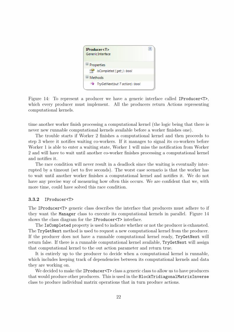
Figure 14: To represent a producer we have a generic interface called IProducer<T>,which every producer must implement. All the producers return Actions representingcomputational kernels.

time another worker finish processing a computational kernel (the logic being that there isnever new runnable computational kernels available before a worker finishes one).

The trouble starts if Worker 2 finishes a computational kernel and then proceeds tostep 3 where it notifies waiting co-workers. If it manages to signal its co-workers beforeWorker 1 is able to enter a waiting state, Worker 1 will miss the notification from Worker2 and will have to wait until another co-worker finishes processing a computational kerneland notifies it.

The race condition will never result in a deadlock since the waiting is eventually inter-rupted by a timeout (set to five seconds). The worst case scenario is that the worker hasto wait until another worker finishes a computational kernel and notifies it. We do nothave any precise way of measuring how often this occurs. We are confident that we, withmore time, could have solved this race condition.

3.3.2 IProducer<T>

The IProducer<T> generic class describes the interface that producers must adhere to ifthey want the Manager class to execute its computational kernels in parallel. Figure 14shows the class diagram for the IProducer<T> interface.

The IsCompleted property is used to indicate whether or not the producer is exhausted.The TryGetNext method is used to request a new computational kernel from the producer.If the producer does not have a runnable computational kernel ready, TryGetNext willreturn false. If there is a runnable computational kernel available, TryGetNext will assignthat computational kernel to the out action parameter and return true.

It is entirely up to the producer to decide when a computational kernel is runnable,which includes keeping track of dependencies between its computational kernels and datathey are working on.

We decided to make the IProducer<T> class a generic class to allow us to have producersthat would produce other producers. This is used in the BlockTridiagonalMatrixInverseclass to produce individual matrix operations that in turn produce actions.

22

3.3.3 The matrix operation producer pattern

Generally, all the classes that implement the IProducer<Action> interface have the follo-wing components:

AbstractOperation an internal class used to represent an abstract operation. It encap-sulates the indices of tiles in the matrix to perform a given operation on. It may also holdan operation type that indicates the mathematical operation to perform. An example ofwhere an operation type is necessary is in the LU Factorization operation, where we needto keep track of whether we are calculating an A, L, U or an LU.

AbstractOperationGenerator a private method that returns an iterator over a se-quence of abstract representations of computational kernels. This sequence is generatedlazily through .nets iterator pattern, instead of having it hardcoded at compile time. Thissaves a lot of memory since only a fraction of the total abstract operations is in memoryat any time.

OperationEnumerator the iterator returned by AbstractOperationGenerator is wrap-ped inside this class. This class has an internal buffer of abstract operations and allowsa caller to retrieve an abstract operation matching a specified predicate. Internally, theproducer will call a method called Find on this class to determine if there are any runnableabstract operations available. The workflow diagram in figure 15 on the following pageillustrates this.

IsRunnable a method used to decide if a given abstract operation is runnable, thatis, the required data is ready. This method is used as the predicate when querying theoperation enumerator. IsRunnable is roughly equivalent to the function DependsOn. Themore complex matrix operations use internal status tables to keep track of the progress.They are updated by the end of a computational kernel and read from the IsRunnablemethod.

GenerateAction a method that converts an abstract operation into an actual compu-tational kernel.

This basic structure is exemplified in figure 16 on page 26.

3.3.4 The straightforward producers

In the category “straightforward producers” we have Multiply, MinusPlusPlus, PlusMultiply,TileOperation, UntileOperation, and SimpleProducer. SimpleProducer is a specialproducer that only produces one computational kernel, a computational kernel it receivesas its argument. It is used in the BlockTridiagonalMatrixInverse producer to do a fewsimple copy operations of data where needed.

23

Is internal buffer

below threshhold?

No

Fill buffer with abstract operations

from AbstractOperationGeneratorYes

Does the buffer contain an

abstract operation matching the

predicate (IsRunnable)

Yes

Returns first

matching abstract

operation and

removes it from

the internal buffer

End

Return nullNo

Call to Find method

(_gen.Find(IsRunnable))

Figure 15: The workflow of the Find method in the OperationEnumerator class. Theinternal buffer threshold is half the buffer size, which is two times the number of physicalcores in the computer.

None of the abovementioned producers have internal status to keep track of intermediateresults and none of them have a specialized operation type.

Since there is no particular order of processing of the individual tiles in the inputdata, the AbstractOperationGenerator in each producer just iterates from one end ofthe output matrix to the other.

The IsRunnable method in each producer merely checks to see if the ingoing tile isready – except for Multiply and PlusMultiply which checks the entire row and columnrequired.

3.3.5 The LUFactorization producer

The LUFactorization producer is a direct implementation of the algorithm described in[Ske09]. The AbstractOperationGenerator produces the suggested optimal computationsequence in section 3.2.1 in [Ske09]. See listing 1 on the following page for our implemen-tation of the AbstractOperationGenerator method.

Each AbstractOperation returned contains an operation type, which can be an LU,L, U, or A, corresponding to lines 1 and 12, 4, 5, and 9 in the pseudocode in figure 3 onpage 12 respectively.

The producer uses an internal status table to keep track of progress. Each positionin the status table contains the time step from figure 3 on page 12, with the value of−1 indicating the completion of the corresponding tile. The status table is used by theIsRunnable method to verify that conditions are met before allowing a computational

24

1 private static IEnumerable < AbstractOperation <OpType >> AbstractOperationGenerator (int N)2 {3 // PDS elimination algorithm from Stigs article §3 .2.14 for (int stage = 1, endStage = 3 * (N - 1) + 1; stage <= endStage ; stage ++)5 {6 // Lower bound : The first sweep completes after 2 ∗N − 1 stages and at each succesive stage another7 // sweep completes . Thus at stage S > 2 ∗N − 1, S − (2 ∗N − 1) sweeps have completed and S − (2 ∗N − 1) + 18 // is the first to be processed .9 // Upper bound : For every third _completed_ stages , a new sweep can start . Thus at stage four

10 // the second sweep can start .11 for (int sweep = System .Math.Max (1, stage - (2 * N - 1) + 1) , endSweep = ( stage - 1) / 3 + 1; sweep <= endSweep ;

sweep ++)12 {13 // generate sweep14 // sweep = is the diagonal sweep number , sweep ∈ [1, N ]15 // tsum = is the sum of the indices in the antidiagonal line to process , tsum ∈ [2 ∗ sweep, 2 ∗N ]16 // tsum is calculated like this : the index sum of elements being processed at stage S17 // is S + 1. Each sweep is one step behind the previous , and thus is at index sum18 // stage + 1− (sweep− 1). ( Sweeps start at one ).19 int tsum = stage + 1 - ( sweep - 1);20 int iMax = System .Math.Min(N, tsum - sweep );21 int iMin = System .Math.Max(tsum - N, sweep );2223 // if it has a diagonal element , do it first24 if (tsum % 2 == 0)25 {26 var i = tsum / 2;2728 if (i == sweep )29 {30 yield return new AbstractOperation <OpType >(i, i, OpType .LU);31 continue ; // jump to start of for loop again32 }33 yield return new AbstractOperation <OpType >(i, i, sweep , OpType .A);34 }3536 if (tsum - sweep <= N)37 {38 // do Lij and Uij second39 yield return new AbstractOperation <OpType >( iMax , sweep , OpType .L);40 yield return new AbstractOperation <OpType >( sweep , tsum - iMin , OpType .U);41 }4243 // walk the anti diagonal with indices tsum− j, j44 // The j index of the sub matrix to be updated using

45 // A(k)i,j

operations is bounded by sweep + 1 and tsum− (sweep + 1)46 // when above the antidiagonal and tsum−N and N when below47 // the antidiagonal .48 for (int j = System .Math.Max( sweep + 1, tsum - N); j <= System .Math.Min(tsum - ( sweep + 1) , N); j++)49 {50 // skip the diagonal , already calculated above51 if (j != tsum - j)52 {53 yield return new AbstractOperation <OpType >( tsum - j, j, sweep , OpType .A);54 }55 }56 }57 }58 }

Listing 1: This listing shows the implementation of the modified PDS algorithm from[Ske09]. Take special note of the “yield return” statements. The yield returnstatements are part of a .net construct called an iterator block. “When a yield returnstatement is reached, the current location is stored. Execution is restarted from thislocation the next time that the iterator is called” (as described in the MSDN library).With all the state management handled by .net, creating the generator as specified in[Ske09] became much easier. Mathematical details are described in the code comments.

25

Figure 16: A collapsed version of the parallel matrix multiply operation. All other matrixoperations have an identical implementation of IsCompleted and TryGetNext.

kernel to be processed.

3.3.6 The MinusMatrixInverseMatrixMultiply producer

As with the LUFactorization producer, we have managed to implement the pipelinedminus – matrix – inverse-matrix multiply algorithm derived in section 2.3.2 on page 13.Listing 2 on page 29 shows our implementation of the scheduling.

Each AbstractOperation returned contains an operation type, which can be an A, Bb,Bc, or C, where A corresponds to line 5 in step 1, Bb corresponds to line 3 and 8 in step1, Bc corresponds to line 5 in step 1 and C corresponds to line 3 and 8 in step 2, fromfigure 5 on page 14.

To keep track of the progress of the intermediate results, we use two status tables, onefor each step. As with LU-factorization, each position in the status table contains the timestep, with the value of −1 indicating the completion of the corresponding tile.

Since it is possible to perform the calculations of each row in parallel, theAbstractOperationGenerator of MinusMatrixInverseMatrixMultiply will not produceAbstractOperations directly, but instead return an AbstractOperationGenerator foreach of the rows in the result matrix. So it is in essence an AbstractOperationGeneratorgenerator. To enable pipelining of the rows we use a special version of theOperationEnumerator class mentioned earlier, PipelinedOperationEnumerator;the PipelinedOperationEnumerator class does this by always trying to find a runnablecomputational kernel in the first row in its pipeline, only looking for runnable computatio-nal kernels in the following rows if that fails.

The internal buffer in the PipelinedOperationEnumerator class is never longer thanthe number of physical cores in the computer, since there is no need to have any moreready to keep all processors busy.

26

3.3.7 The Inverse producer

As noted in 2.3.3 on page 14, the matrix inverse scheduling follow the same pattern as theminus – matrix – inverse-matrix multiply scheduling.

From an implementation standpoint, they are also quite similar. It also uses twointernal status tables to keep track of progress. The AbstractOperationGenerator ofthe matrix inverter producer is also an AbstractOperationGenerator generator, theonly difference is that the AbstractOperationGenerators that are generated generatesAbstractOperations over each column in the result matrix, instead of each row, otherwiseit is the same concept.

Each AbstractOperation returned contains an operation type, which can be either aF, R, G, or H, where F corresponds to line 3 and line 8 in step 1, R corresponds to line5 in step 1, G corresponds to line 3 and 8 in step 2 and H corresponds to line 5 in step 2(see psuedocode in figure 7 on page 15).

The code in listing 3 on page 30 displays the AbstractOperationGenerators.

3.3.8 The BlockTridiagonalMatrixInverse producer

To calculate the inverse of a block tridiagonal matrix we use theBlockTridiagonalMatrixInverse producer. It differs from the other producers in that itproduces other producers – i.e. the previously mentioned matrix operations, and is thusnot directly compatible with the Manager class.The PipelinedBlockTridiagonalMatrixInverse andNonPipelinedBlockTridiagonalMatrixInverse classes are wrappers that acts as an in-termediate between the Manager class and the BlockTridiagonalMatrixInverse produ-cer. As the names suggest, the first tries to pipeline the matrix operations coming fromBlockTridiagonalMatrixInverse, while the latter does not.

The non pipelined wrapper does not advance to the next matrix operation until thecurrent one is completed. The pipelined wrapper keeps two matrix operations at hand,issuing runnable computational kernels from the secondary only when none are availablefrom the primary. When the primary is completed, the secondary is promoted and a newone is retrieved in its place.

Because of the serial nature of the calculations of formulae (1) through (6), we decidedto have only two operations in the pipeline since there will almost never be any runnablecomputational kernels available in a third matrix operation.

We have chosen to implement a straightforward scheduling for the computation of theformulae from section 2.1 on page 9. The first operation is a tile operation, after thatcomes the upward sweep followed by the downward sweep and then the final calculations.Once everything is done we untile the block tridiagonal matrix again.

In order to pipeline matrix operations, they need to be created before their input dataexists. This poses a challenge since it requires a pointer to the future location of the inputdata. We solved this with the OperationResult class mentioned in 3.2 on page 20. It canbe shared between different matrix operations, one using it to save the result in and one

27

or more using it as input.The IsCompleted property and the bit table of the OperationResults class are used

to communicate the status of the entire block matrix or individual tiles in the block matrixbetween matrix operations. There need not be data embedded in an OperationResult,it can simply exist as a link between matrix operations until one of them decides to fill indata and update the appropriate status.

3.3.9 Possible improvements and issues

Many of the obvious improvements we see are related to pipelining.When it comes to memory usage we are quite wasteful, performing almost none of

the calculations inplace and keeping the results of the upward and downward sweeps inmemory through the entire block tridiagonal matrix inverse computation. If we where toanalyse the individual computations closer we would be able to determine when it is safeto throw away unneeded intermediate results, as well as which would be suitable as inplaceoperations.

Another realm we see possibilities in is how aggressive some of the matrix operationsare about starting their calculations. Currently MinusMatrixInverseMatrixMultiply,Inverse, and LUFactorize all wait until their entire input is ready. In theory, they couldstart computation as soon as the required number of tiles is ready from the previous matrixoperation. This is not trivial though, since one matrix operation has to be absolutelysure it does no longer need a tile in its result before flagging it as done. Otherwise,subsequent matrix operations performing inplace operations might alter the data affectingthe calculations of the remaining tiles in the previous matrix operation.

When comparing the results of a single threaded tiled block tridiagonal matrix inversionwith the results of the one in parallel, the two sometimes differ by around 1.0E−10. Webelieve that this is due to unintended reordering of computational kernels. A finer grainedtuning of when the different matrix operations assume its input data is ready should solvethis inaccuracy.

There is also the already mentioned issue with the race condition in the GetWork me-thod (see 3.3.1 on page 21) that might give us a slight speedup in general during paralleloperations if fixed.

All of the above issues seem within our grasp, the only thing missing is time.

28

1 private static IEnumerable < OperationEnumerator < AbstractOperation <OpType >>> AbstractOperationGenerator (int M, int N)2 {3 for (int i = 1; i <= M; i++)4 {5 yield return new OperationEnumerator < AbstractOperation <OpType >>( B_RowActionGenerator (i, N),

Constants . MAX_QUEUE_LENGTH );6 }78 for (int i = 1; i <= M; i++)9 {

10 yield return new OperationEnumerator < AbstractOperation <OpType >>( C_RowActionGenerator (i, N),Constants . MAX_QUEUE_LENGTH );

11 }12 }1314 // Implementation of PIM algorithm from [ Ske09 ], figure 7.15 private static IEnumerable < AbstractOperation <OpType >> B_RowActionGenerator (int i, int N)16 {17 for (int step = 1; step <= 2 * (N - 1) + 1; step ++)18 {19 // The first N steps , sweep 1 is the first .20 // From then on one sweep is completed at every step .21 int sweep = System .Math.Max (0, step - N);22 for (int j = System .Math.Min(step , N); j >= step / 2 + 1; j--)23 {24 sweep ++;25 if (j == sweep )26 {27 // First operation is Bij28 yield return new AbstractOperation <OpType >(i, j, j, OpType .Bb);29 }30 else31 {

32 // The rest are A(sweep)ij

operations

33 yield return new AbstractOperation <OpType >(i, j, sweep , OpType .A);34 }35 }36 }37 }3839 // A PIM based on [ Ske09 ] figure 7, but moving right to left .40 // See the minus matrix inverse matrix multiply scheduling figure elsewhere in this paper .41 private static IEnumerable < AbstractOperation <OpType >> C_RowActionGenerator (int i, int N)42 {43 for (int step = 1; step <= 2 * (N - 1) + 1; step ++)44 {45 int sweep = System .Math.Max (0, step - N);4647 // As seen in [ Ske09 ] figure 7, the first N steps the j48 // index start at step, the rest of the steps j starts49 // at N . It then counts down to , as seen in the figure , sweep/2 + 1.50 for (int j = System .Math.Max(N - (step - 1) , 1); j <= N - (step / 2); j++)51 {52 sweep ++;53 if (j == N - ( sweep - 1))54 {55 yield return new AbstractOperation <OpType >(i, j, sweep , OpType .C);56 }57 else58 {59 yield return new AbstractOperation <OpType >(i, j, sweep , OpType .Bc);60 }61 }62 }63 }

Listing 2: This listing shows the implementation of the minus – matrix – inverse-matrixmultiply scheduling algorithm.

29

1 private static IEnumerable < OperationEnumerator < AbstractOperation <OpType >>> AbstractOperationGenerator (int N)2 {3 for (int i = 1; i <= N; i++)4 {5 yield return new OperationEnumerator < AbstractOperation <OpType >>( F_ColumnAbstractActionGenerator (i, N),

Constants . MAX_QUEUE_LENGTH );6 }78 for (int i = 1; i <= N; i++)9 {

10 yield return new OperationEnumerator < AbstractOperation <OpType >>( G_ColumnAbstractActionGenerator (i, N),Constants . MAX_QUEUE_LENGTH );

11 }12 }1314 // A generator for the schedule of Inverse step 1. It is the15 // same schedule as that of minus matrix inverse matrix multiply , except16 // that i and j are interchanged17 // and some elements are skipped as they do not contribute to the result .18 private static IEnumerable < AbstractOperation <OpType >> F_ColumnAbstractActionGenerator (int j, int N)19 {20 // Sweeps starting at elements above the diagonal are skipped21 // by starting at the step where sweep j starts .22 for (int step = 2 * (j - 1) + 1; step <= 2 * (N - 1) + 1; step ++)23 {24 // Skip to sweep j25 int sweep = System .Math.Max(j - 1, step - N);2627 // For the N steps , j − 1 rows28 // are skipped .29 for (int i = System .Math.Min(step - (j - 1) , N); i >= step / 2 + 1; i--)30 {31 sweep ++;32 if (i == sweep )33 {34 // The timestep ( third parameter ) is moved to begin at 1.35 yield return new AbstractOperation <OpType >(i, j, sweep - (j - 1) , OpType .F);36 }37 else38 {39 // The timestep ( third parameter ) is moved to begin at 1.40 yield return new AbstractOperation <OpType >(i, j, sweep - (j - 1) - 1, OpType .R);41 }42 }43 }44 }4546 // A generator for the schedule of Inverse step 2. It is identical to the scheduler47 // of minus matrix inverse matrix multiply step 2, with i and j48 // interchanged .49 private static IEnumerable < AbstractOperation <OpType >> G_ColumnAbstractActionGenerator (int j, int N)50 {51 for (int step = 1; step <= 2 * (N - 1) + 1; step ++)52 {53 int sweep = System .Math.Max (0, step - N);54 for (int i = System .Math.Max(N - (step - 1) , 1); i <= N - (step / 2); i++)55 {56 sweep ++;57 if (i == N - ( sweep - 1))58 {59 yield return new AbstractOperation <OpType >(i, j, sweep , OpType .G);60 }61 else62 {63 yield return new AbstractOperation <OpType >(i, j, sweep - 1, OpType .H);64 }65 }66 }67 }

Listing 3: This listing shows the implementation of the block matrix inverse schedulingalgortihm.

30

4 Performance measurementsIn this section we will present our performance measurements, the results they producedand a discussion of these. To keep the main report within a tolerable length, we try tolimit the number of tables and graphs, and refer to the appendix as well as the online copyor the attached media for all our test results. Only results deemed important are included,but most if not all are discussed.

4.1 Experiment setupDuring the first months of development we only had access to a laptop with an Intel CoreDue 2 processor, limiting our testing ability. Later in the process we gained access to aneight core machine due to Brian Vinter and the Minimum intrusion Grid (MiG)2 team atDIKU, which we are very grateful for. All our results presented in this section are basedon experiments performed on this computer.

Hardware (DIKUs MiG eight core system):

• 2 x Intel Xeon Processor E5310 @ 1.6 GHz, with 8 MB Level 2 cache, 128 KB Level1 cache

• 8 GB RAM

• Running Linux 2.6.28-14-server Ubuntu SMP

• Mono version 2.0.1

Our software platform is the Microsoft.NET3 platform, but we are able run our codewithout too many problems on Linux through the Mono4 runtime. We did run into afew issues with the version of Mono installed in DIKUs system; specifically, the garbagecollector would crash when we tried to perform measurements with very large datasets.The issue is fixed in a later version of Mono but unfortunately, it was not possible to installthat on the test computer.

Another limitation with our setup is that we were physically unable to disable a certainnumber of cores. We desired to run our measurements with 1, 2, 4, 6, and 8 threads active,and had we been able to disable for example four of the cores when running measurementswith four threads, the impact of other processes needing CPU time would be equalled out.With that said, we do not consider this a big issue but it is noteworthy nonetheless.

Table 1 on the following page lists all the experiments we performed. All experimentswere conducted in both single threaded, single threaded tiled and parallel modes. For

2www.migrid.org3www.microsoft.com/NET/4www.mono-project.com - An open source, cross-platform, implementation of C# and the CLR that is

binary compatible with Microsoft.NET.

31

the parallel modes, all measurements were run with 1, 2, 4, 6, and 8 threads. For bothsingle threaded tiled and parallel mode the tile size used ranged from 10 to 150. Someexperiments were not feasible or meaningful with some tile sizes, either because the runningtime became too short or because Mono would crash when a small tile size resulted in toomany tiles, i.e. objects, in memory.

We use the following notation in this section:

• BTM is short for Block Tridiagonal Matrix

• 100x150x250 means BTM with 100 elements along the diagonal, giving a total of 298(3 ∗ 100− 2) elements. Each element is a block matrix of a random size between 150and 250 containing random numbers.

• 5000x5000 means a matrix of 5000 by 5000 elements (numbers), all random values.

Operation BTM Matrix SizeLU-factorization −

√3000x3000

Inverse −√

2500x2500Minus – matrix – inverse-matrix multiply −

√2500x2500

PlusMultiply −√

2500x2500Multiply −

√2500x2500

MinusPlusPlus −√

5000x5000Block Tridiagonal Matrix Inverse

√− 50x100x200

Block Tridiagonal Matrix Inverse√

− 200x100x200Block Tridiagonal Matrix Inverse

√− 100x50x100

Block Tridiagonal Matrix Inverse√

− 100x100x200Block Tridiagonal Matrix Inverse

√− 100x150x250

Block Tridiagonal Matrix Inverse√

− 10x500x500Block Tridiagonal Matrix Inverse

√− 10x750x750

Table 1: Overview of experiments and matrix sizes used.

There is an obvious upper bound on how large we can make in particular the blocktridiagonal matrices for testing due to the previously mentioned Mono bug, for example, ablock tridiagonal matrix of 100x300x500 would not run. Instead, we reduced the numberof block matrices, allowing us to increase the block size.

We were also unable to run the individual matrix operations with larger datasets thanthose specified. Smaller datasets resulted in very short running times, which did not yieldany conclusive results. Nonetheless the chosen sizes are within the magnitude set forth in[Ske09].

32

Statistics gathered during measurements The statistics gathered during our mea-surements include the following:

• The total running time of the operation

• The number of threads used (parallel mode only)

• The tile size used (single threaded tiled and parallel mode only)

• The total number of computational kernels processed (parallel mode only)

• The total number of times workers failed to retrieve a runnable computational kernelfrom the producer (parallel mode only)

• The total number of times workers received a runnable computational kernel from thesecondary producer (only in parallel pipelined mode – i.e. block tridiagonal matrixinversion).

Besides allowing us to calculate speedups, we also use the following formulae:

Speedup = running time of baseline implementationrunning time of experiment

% times workers did not receive work =#times failed to get work

(#times failed to get work + #computational kernels)

% computational kernels pipelined =#times received work from secondary producer

#computational kernelsFor two of the block tridiagonal matrix inversion experiments, we also logged:

• The total running time in ticks

• The total number of ticks workers slept, waiting for another worker to notify themof possible new available computational kernels.

• The total number of ticks workers spent spinning, waiting to be allowed to requesta computational kernel (the spin wait lock around the TryGetWork method in theproducer).

33

The above statistics allowed us to calculate percentage of time spent sleeping as well asthe percentage of time spent contending the spin wait lock. These are calculated like this:

% spinning time = #ticks spinning#threads× running time in ticks

% sleeping time = #sleeping ticks#threads × running time in ticks

Since the total running time is not based on how many ticks the program actually used,but rather the amount of ticks that passed during the entire execution of the experiment,the above formulae present the best case scenario, where none of the threads are interruptedby the operating system or other components in the runtime like the garbage collector.Nevertheless, we feel they are still valid and bring good insight into the overhead causedby our scheduling algorithms.

4.2 Experiment results and analysisIn table 2 we present the best possible speedups achieved in the different matrix operations,as well as the configuration used. In the following subsections we will go into the resultfrom the experiments for each matrix operation.

Matrix operation Tile size Matrix orBTM size

Best speedup

LU-factorization 100 3000x3000 7.734Inverse 90 2500x2500 7.742Minus – matrix – inverse-matrix multiply 90 2500x2500 7.772PlusMultiply 150 2500x2500 7.838Multiply 150 2500x2500 7.858MinsPlusPlus 10 5000x5000 2.716Block Tridiagonal Matrix Inverse 80 10x750x750 7.348

Table 2: Overview of best achieved speedups using 8 threads. It turned out to be veryhard to achieve speedups with a larger number of threads in the MinusPlusPlus operatoin.The speedup in the table was logged with only two threads active. We discuss the issueswith MinusPlusPlus in section 4.2.3 on page 39

For a baseline comparison, we used the results collected from the single threaded andsingle threaded tiled implementations. Interestingly, going from a non-tiled to a tiledimplementation yields significant speedups. The table 3 on the following page shows theinitial speedups we attain going from non-tiled to tiled.

The reason for the speedups we get when tiling may be that the processor keeps theindividual tiles in local cache longer while performing calculations, limiting the overheadof communication between main memory and the CPU, resulting in better utilization ofthe processor caches.

34

Matrix operation Tile size Matrix orBTM size

Speedup

LU-factorization 50 3000x3000 2.110Inverse 40 2500x2500 4.329Minus – matrix – inverse-matrix multiply 50 2500x2500 5.085PlusMultiply 60 2500x2500 2.776Multiply 60 2500x2500 2.793MinusPlusPlus 100 5000x5000 5.065Block Tridiagonal Matrix Inverse 40 10x750x750 2.368

Table 3: Single threaded to single threaded tiled speedups

Tiling is not always the best solution though. On DIKUs computer, where the processorhas a rather large L1 cache available, the added overhead of tiling results in slowdownswhen the blocks in a block tridiagonal matrix gets below approximately 150x150.

4.2.1 Presentation and analysis of LU-factorization

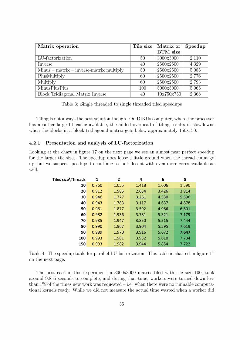
Looking at the chart in figure 17 on the next page we see an almost near perfect speedupfor the larger tile sizes. The speedup does loose a little ground when the thread count goup, but we suspect speedups to continue to look decent with even more cores available aswell.

Tiles size\Threads 1 2 4 6 8

10 0.760 1.055 1.418 1.606 1.590

20 0.912 1.585 2.634 3.426 3.914

30 0.946 1.777 3.261 4.530 5.596

40 0.943 1.783 3.117 4.637 4.878

50 0.961 1.877 3.592 4.966 6.601

60 0.982 1.936 3.781 5.321 7.179

70 0.985 1.947 3.850 5.515 7.444

80 0.990 1.967 3.904 5.595 7.619

90 0.989 1.970 3.916 5.672 7.647

100 0.993 1.981 3.932 5.610 7.734

150 0.993 1.982 3.944 5.854 7.722

Table 4: The speedup table for parallel LU-factorization. This table is charted in figure 17on the next page.

The best case in this experiment, a 3000x3000 matrix tiled with tile size 100, tookaround 9.855 seconds to complete, and during that time, workers were turned down lessthan 1% of the times new work was requested – i.e. when there were no runnable computa-tional kernels ready. While we did not measure the actual time wasted when a worker did

35

3

4

5

6

7

8

Speedup

10

20

40

50

60

70

100

0

1

2

3

4

5

6

7

8

1 2 4 6 8

Speedup

Threads

10

20

40

50

60

70

100

150

Perfect

Figure 17: Speedup chart for parallel LU-factorization. Note that some tile sizes arefiltered out to make the chart more readable, the full dataset can be found in table 4 onthe previous page

not receive work from the LU-factorize producer, the very low number of “misses” gives usa strong indication that the modified PDS algorithm presented in [Ske09] and reiteratedin section 2.3.1 on page 11 does indeed work well.

We clearly see that the smaller tile sizes are not able to produce a respectable speedup.Even though workers were almost never turned down asking for work (1.22E-6% of thetime for tile size 10, or in numbers, 11 times out of 9,045,061), the large amount of smalltiles resulted in very fast computational kernels and a lot more scheduling. The smallertile sizes also resulted in poor utilization of processor cache, by not coming close to fillingthe cache, which certainly did not help running times either.

With larger datasets it is possible that we could have produced slightly better speedups.With smaller datasets we saw speedups drop when the matrix size came close to the tilesize, for example in the case of a 150x150 block matrix. This is expected as the overhead ofscheduling takes a more significant amount of time and there are fewer tiles than workers.

Running times and other statistics are printed in the appendix in table 23 on page 62.

36

4.2.2 Presentation and analysis of Inverse and Minus – Matrix – Inverse-Matrix Multiply

Our experiments with Inverse and Minus – Matrix – Inverse-Matrix Multiply yielded verysimilar results (and oddities), so we will look at them together. Considering the similarnature of their implementation, this is no surprise.

In general, tile sizes in the range of 70 to 150 all resulted in speedups above 7.4, andspeedups are, as with LU-factorization, close to perfect with those tile sizes.

As the charts in figure 19 on page 39 and figure 18 reveal, we calculated the speedupbased on the results of our parallel implementation running with one thread. We did thisbecause our parallel implementation actually produced better running times with just onethread than the single threaded tiled version.

3

4

5

6

7

8

Speedup

10

20

30

40

50

90

0

1

2

3

4

5

6

7

8

1 2 4 6 8

Speedup

Threads

10

20

30

40

50

90

150

Perfect

Figure 18: Speedup chart for parallel Inverse. Note that some tile sizes are filtered out tomake the chart more readable, the full dataset can be found in table 5 on the next page

The speedup from the single threaded tiled version to the parallel version using onethread is 1.4 on average over all tile sizes, and comparing the single threaded tiled versionto the parallel version running with eight threads yielded speedups above 10.0, in the case

37

Tile size\Threads 1 2 4 6 8

10 1.000 1.364 1.863 2.131 2.076

20 1.000 1.733 2.979 3.877 4.511

30 1.000 1.886 3.481 4.864 6.131

40 1.000 1.847 3.654 4.891 6.488

50 1.000 1.952 3.827 5.568 7.178

60 1.000 1.973 3.859 5.679 7.420

70 1.000 1.992 3.933 5.800 7.606

80 1.000 1.992 3.945 5.830 7.707

90 1.000 1.990 3.954 5.863 7.742

100 1.000 1.993 3.961 5.868 7.630

150 1.000 1.995 3.935 5.779 7.531

Table 5: The speedup table for parallel Inverse. This table is charted in figure 18 on theprevious page.

Tile size\Threads 1 2 4 6 8

10 1.000 1.429 1.878 2.131 2.090

20 1.000 1.716 2.899 3.777 4.389

30 1.000 1.893 3.491 4.871 6.023

40 1.000 1.943 3.358 4.738 5.661

50 1.000 1.984 3.780 5.585 7.067

60 1.000 1.988 3.870 5.673 7.398

70 1.000 1.994 3.934 5.824 7.642

80 1.000 1.993 3.954 5.863 7.718

90 1.000 1.995 3.967 5.887 7.772

100 1.000 1.998 3.974 5.905 7.733

150 1.000 1.994 3.949 5.880 7.667

Table 6: The speedup table for parallel Minus – Matrix – Inverse-Matrix Multiply. Thistable is charted in figure 19 on the next page.

of Inverse, and above 11.5 with Minus – Matrix – Inverse-Matrix Multiply.One possible explanation could be that the scheduling implemented in the parallel

version has an effect even with only one thread in play. The order in which the different tilesare computed may result in less communication between processor and memory, resultingin better speed. Also, very little synchronisation is required when only one thread isrunning.

Another reason could be a less than optimal single threaded tiled implementation ofInverse and Minus – Matrix – Inverse-Matrix Multiply on our part, even though we producesignificant speedups compared to our non-tiled implementation.

Oddities aside, we do think that the PIM algorithm presented in [Ske09] has provenitself, at least with our experiment setup. With the tile sizes that resulted in the best

38

3

4

5

6

7

8

Speedup

10

20

30

40

50

60

70

80

0

1

2

3

4

5

6

7

8

1 2 4 6 8

Speedup

Threads

10

20

30

40

50

60

70

80

90

100

150

Perfect

Figure 19: Speedup chart for parallel Minus – Matrix – Inverse-Matrix Multiply. Notethat some tile sizes are filtered out to make the chart more readable, the full dataset canbe found in table 6 on the previous page

speedups, the number of times a worker did not get a runnable computational kernel fromthe producer was less than 2% in both operations, with a total running time at around 11seconds for Inverse and 16 seconds for Minus – Matrix – Inverse-Matrix Multiply.

Running times and other statistics are printed in the appendix in table 24 on page 63and in table 25 on page 64.

4.2.3 Presentation and analysis of Multiply, Plus Multiply, Minus Plus Plus

Both Multiply and Plus Multiply have near optimal speedups of about 7.8, which is nobig surprise since they are both delightfully parallel. We note that both keep all threadsbusy at all time; there is no waiting for runnable computational kernels at any time duringexecution. See table 27 on page 66 and table 28 on page 67 for running times and otherstatistics.

We also expected great speedups for our Minus Plus Plus operation, but it turns out

39

that running it in parallel did not produce good results at all. 2.716 was best speedupachieved with a tile size of 10 using 6 threads. Actually, anything above two threads resultsin disappointing speedups; it was especially bad with eight threads where we actuallymanaged to get a slowdown. Table 26 on page 65 reveals the dreadful results.

The obvious reason lies in the fact that the running time of computational kernels toscheduling overhead ratio is too small, due to the simple nature of the minus and plusmatrix operations. We might have been able to get better measurement results if we hadbeen able to run with a larger dataset; this was not possible due to Mono crashing whena large number of objects are created in memory.

In practice, we suspect that one would need a very large matrix – say in the rangeof 15000x15000 to see a significant speedup with more than a few threads. A matrix of5000x5000 used in our experiments only took our single threaded tiled implementation 0.9seconds to complete, not leaving much room for parallelization. In cases with block sizes inthe lower thousands, as are the practical use cases reported in [Ske09], one might considernot running MinusPlusPlus in parallel at all.

4.2.4 Presentation and analysis of Block Tridiagonal Matrix Inversion

For the block tridiagonal matrix inversion experiments we varied the number of blocks aswell as their size. The best speedup with eight threads in each experiment is displayed intable 7.

BTM size Tile size Speedup100x50x100 30 1.84750x100x200 40 4.258100x100x200 35 4.545200x100x200 35 4.604100x150x250 40 5.57110x500x500 90 7.17410x750x750 80 7.348

Table 7: Summary of best speedups attained with eight threads in the different experimentsconducted.

Looking at the summary table, we clearly see a pattern. Block sizes have great impacton the speedup, while the number of blocks has negligible impact.

When running with only 4 threads, we see decent speedups of around 3.1 on lower blocksizes as well. The chart in figure 20 on the following page illustrates this. It shows thebest possible speedup achieved for all BTM sizes as a function of thread count. All but100x50x100 is able to produce a speedup of over 3.0 with 4 threads. Raising the threadcount, only BTMs with blocks bigger than 500x500 are able to retain the growth of theirspeedup.

40

This is not a surprising result considering the small amount of tiles produced whentiling the smaller block matrices. Tiling a block matrix of size 150x150 with a tile size of30 only results in 5 blocks, making it hard to keep more than 4 workers busy.

4

5

6

7

8

Speedup

100x50x100

50x100x200

100x100x200

200x100x200

100x150x250

0

1

2

3

4

5

6

7

8

1 2 4 6 8

Speedup

Threads

100x50x100

50x100x200

100x100x200

200x100x200

100x150x250

10x500x500

10x750x750

Perfect

Figure 20: Speedup chart for parallel Block Tridiagonal Matrix Inversion.

If we take a closer look at the numbers gathered in our best case scenario, we processeda 10x750x750 BTM tiled with a tile size of 80, in 35.676 seconds resulting in a speedup of7.348. That tile size resulted in 10 tiles per block, which in turn resulted in workers gettingturned down for runnable computational kernels 9.492% of the time they asked. However,only 3% of the total running time was actually spent sleeping – waiting for other workersto notify them of possible new work being available – and only 0.5% of the running timewas spent spinning while waiting their turn to ask the producer for work.

The statistics collected running with a BTM of size 100x100x200, tiled with tile size35, explains the poor speedup of 4.545. With an average of 5 tiles in each block, the eightthreads did not receive runnable computational kernels 31.16% of the time they requestedit and spent 11.06% of their time sleeping. Those numbers are not surprising since thereare eight workers contending for five tiles in each block. We also registered a large 15.03%of time spent spin waiting for the producer lock, which makes sense since more workers will

41

arrive at the spin wait lock at the same time due to being woken up by workers completingwork.

Full tables with all the cited data can be found in appendix A on page 46.

4.3 Possible improvementsWhile we are happy with the speedups we are able to produce for block tridiagonal matrixinversion, we do see a few obvious areas where we could improve things.

As already mentioned, the attempt at parallelizing the minus plus plus operation shouldbe reconsidered. It speaks in its favour that it is very pipeline friendly; it can startcomputation on the individual tiles in its input as soon as they are ready, and as soon asa tile in a its result matrix is finished, a following matrix operation can start its work onthat particular tile.

In contrast LU-factorization, Inverse and Minus – Matrix – Inverse-Matrix Multiply alllack proper pipelining capabilities. In their current state they have to wait until all theirinput is completely ready before beginning their computations. The reason for this is thatthey all clone their input and perform the calculations inplace on the clone. We believe wecan alleviate this without changing the general design of our framework given more time.

Besides making some of the matrix operations more pipeline friendly, we could look intobreaking apart the serial nature of the tridiagonal block inversion algorithm by interleavingthe operations that do not depend on each other. For example, the upward and downwardsweeps could be interleaved as they are completely independent.

In general we have observed that BTM operations are not pipelined very much. Weexpect both enhancements mentioned above to improve on this. In particular we expectavoiding operation interdependencies to give good results. BTMs with smaller block sizes– i.e. few tiles – will benefit the most from improved pipelining.

Another improvement that all matrix operations probably could benefit from, is tocompletely remove the sleeping state a worker can enter if it does not receive any workfrom the producer; instead of going to sleep it simply retries until receiving a computa-tional kernel, or the producer completes. This would eliminate the notification step afterthe processing of a computational kernel and get rid of the race condition mentioned insection 3.3.1 on page 21.

Continuing on that path, designing a manager without a lock around the call to theTryGetWork method could be an adventurous undertaking. The benefits of this might bemore significant if the amount of workers (i.e. cores) goes from eight to 16, 32 or evenhigher. A solution based on a lock free implementation of a linked list or priority queuecould be an option. We toyed with a few designs during development, but optimizationsperformed by the .net compiler and CPU at runtime, like reordering of read and writeinstructions in some conditions, makes it hard at best to write lock free code, and evenmore difficult to verify.

42

4.4 What could have beenOur measurements are far from comprehensive; here are some of the things we would haveliked to measure had time allowed:

• Measure the total time spent processing computational kernels (in ticks).

• Measure the total time spent retrieving computational kernels from the producer(this would allow us to better calculate the overhead of the scheduling).

• Measure the actual CPU utilization during execution.

• Measure the cache hit-miss ratio during execution.

With the above data, it would have been possible to get a better idea of how muchtime was spent during execution by other things like garbage collection, other processesoutside our program or the OS itself.

We are, however, uncertain if measuring CPU utilization, cache hit-miss ratio, andadvanced profiling in general is possible on the MiG system.

It would also have been great to run all the parallel experiments with the extra ticksstatistics we only had time to gather for a few selected BTM experiments. Obviously, awider range of experiments, especially larger block sizes and higher tile sizes, would havebeen interesting.

While we do not expect there to be any noteworthy overhead of pipelining individualblocks in a BTM, it would have been good to confirm this. As mentioned in section 4.1on page 31, the issues with Mono prevented us from playing much with number of blockswhile using larger block sizes, so even though DIKUs computer has enough memory toallow us to compute a BTM of 50x750x750 or even 100x750x750, Mono would not playnice.

On the hardware side, it would have been of great interest to run our performancemeasurements on different hardware, in particular hardware with more than eight cores.

43

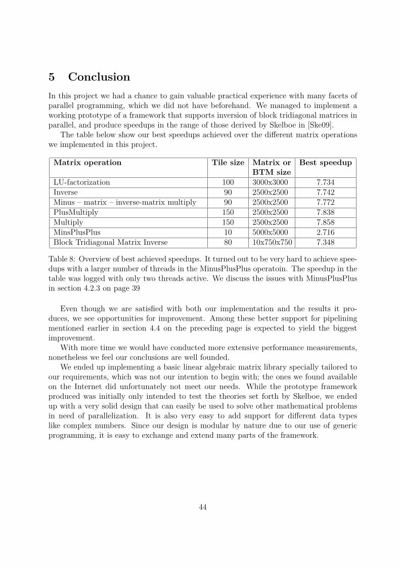
5 ConclusionIn this project we had a chance to gain valuable practical experience with many facets ofparallel programming, which we did not have beforehand. We managed to implement aworking prototype of a framework that supports inversion of block tridiagonal matrices inparallel, and produce speedups in the range of those derived by Skelboe in [Ske09].

The table below show our best speedups achieved over the different matrix operationswe implemented in this project.

Matrix operation Tile size Matrix orBTM size

Best speedup

LU-factorization 100 3000x3000 7.734Inverse 90 2500x2500 7.742Minus – matrix – inverse-matrix multiply 90 2500x2500 7.772PlusMultiply 150 2500x2500 7.838Multiply 150 2500x2500 7.858MinsPlusPlus 10 5000x5000 2.716Block Tridiagonal Matrix Inverse 80 10x750x750 7.348

Table 8: Overview of best achieved speedups. It turned out to be very hard to achieve spee-dups with a larger number of threads in the MinusPlusPlus operatoin. The speedup in thetable was logged with only two threads active. We discuss the issues with MinusPlusPlusin section 4.2.3 on page 39

Even though we are satisfied with both our implementation and the results it pro-duces, we see opportunities for improvement. Among these better support for pipeliningmentioned earlier in section 4.4 on the preceding page is expected to yield the biggestimprovement.

With more time we would have conducted more extensive performance measurements,nonetheless we feel our conclusions are well founded.

We ended up implementing a basic linear algebraic matrix library specially tailored toour requirements, which was not our intention to begin with; the ones we found availableon the Internet did unfortunately not meet our needs. While the prototype frameworkproduced was initially only intended to test the theories set forth by Skelboe, we endedup with a very solid design that can easily be used to solve other mathematical problemsin need of parallelization. It is also very easy to add support for different data typeslike complex numbers. Since our design is modular by nature due to our use of genericprogramming, it is easy to exchange and extend many parts of the framework.

44

References[PSH+08] Dan Erik Petersen, Hans Henrik B. Sørensen, Per Christian Hansen, Stig Skel-

boe, and Kurt Stokbro. Block tridigonal matrix inversion and fast transmissioncalculations. Journal of Computational Physics, pages 3174–3190, 2008.

[Ske09] Stig Skelboe. The scheduling of a parallel tiled matrix inversion. 2009.

45

A Measurement resultsIn this section we list all the statistics gathered which are mentioned in the report. Boththose listed here and even more may be found online at http://github.com/egil/Inversion-of-Block-Tridiagonal-Matrices/tree/master/Rapport/Experiments/ or on the CD accom-panying this report.

• BTM 10x750x750 - collected statistics: table 9 on page 48

• BTM 10x750x750 - calculated statistics: table 10 on page 49

• BTM 10x750x750 - measurement including extra statistics - collected statistics part1: table 11 on page 50

• BTM 10x750x750 - measurement including extra statistics - collected statistics part2: table 12 on page 51

• BTM 10x750x750 - measurement including extra statistics - calculated statistics:table 13 on page 52

• BTM 10x500x500 - collected statistics: table 14 on page 53

• BTM 10x500x500 - calculated statistics: table 15 on page 54

• BTM 100x100x200 - measurement including extra statistics - collected statistics:table 16 on page 55

• BTM 100x100x200 - measurement including extra statistics - calculated statistics:table 17 on page 56

• BTM 100x100x200 - collected and calculated statistics: table 18 on page 57

• BTM 100x50x100 - collected and calculated statistics: table 19 on page 58

• BTM 100x150x250 - collected and calculated statistics: table 20 on page 59

• BTM 200x100x200 - collected and calculated statistics: table 21 on page 60

• BTM 50x100x200 - collected and calculated statistics: table 22 on page 61

• LU-factorization: 3000x3000 - collected and calculated statistics: table 23 on page 62

• Inverse: 2500x2500 - collected and calculated statistics: table 24 on page 63

• Minus – Matrix – Inverse-Matrix Multiply: 2500x2500 - collected and calculatedstatistics: table 25 on page 64

• MinusPlusPlus: 5000x5000 - collected and calculated statistics: table 26 on page 65

46

• Multiply: 2500x2500 - collected and calculated statistics: table 27 on page 66

• PlusMultiply: 2500x2500 - collected and calculated statistics: table 28 on page 67

47

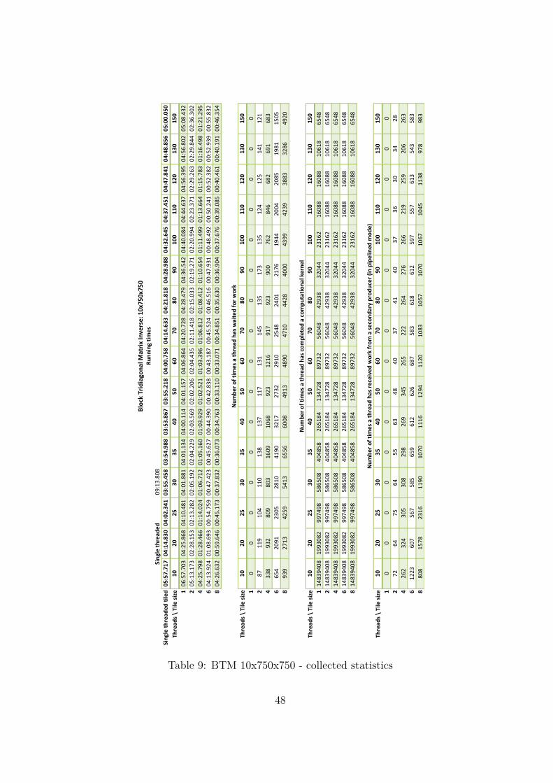
09:13.808

Sin

gle

thre

ade

d t

iled

05

:57

.71

70

4:1

4.8

30

04

:02

.34

10

3:5

5.4

58

03

:54

.98

80

3:5

3.8

67

03

:55

.21

80

4:0

0.7

58

04

:14

.63

30

4:2

1.8

18

04

:28

.98

80

4:3

2.6

45

04

:37

.45

10

4:4

7.8

41

04

:48

.85

60

5:0

0.0

50

Thre

ads

\ Ti

le s

ize

10

20

25

30

35

40

50

60

70

80

90

10

01

10

12

01

30

15

0

106:57.703

04:25.868

04:10.481

04:01.881

04:01.134

04:00.114

04:01.157

04:06.864

04:20.728

04:28.479

04:36.542

04:40.084

04:44.637

04:56.395

04:56.802

05:08.432

205:13.173

02:28.153

02:13.282

02:05.192

02:04.229

02:03.569

02:02.206

02:04.435

02:11.418

02:15.033

02:19.271

02:20.994

02:23.371

02:29.263

02:29.844

02:36.302

404:25.798

01:28.466

01:14.024

01:06.712

01:05.160

01:03.929

01:02.521

01:03.396

01:06.812

01:08.412

01:10.654

01:11.499

01:13.664

01:15.783

01:16.498

01:21.295

604:13.924

01:08.693

00:54.759

00:47.423

00:45.627

00:44.390

00:42.838

00:43.187

00:45.524

00:46.516

00:47.931

00:48.492

00:50.241

00:52.382

00:52.939

00:55.832

804:26.632

00:59.646

00:45.173

00:37.832

00:36.073

00:34.763

00:33.110

00:33.071

00:34.851

00:35.630

00:36.904

00:37.676

00:39.085

00:40.461

00:40.191

00:46.354

Thre

ads

\ Ti

le s

ize

10

20

25

30

35

40

50

60

70

80

90

10

01

10

12

01

30

15

0

10

00

00

00

00

00

00

00

0

287

119

104

110

138

137

117

131

145

135

173

135

124

125

141

121

4338

932

809

803

1609

1068

923

1216

917

923

900

762

846

682

691

683

6654

2091

2305

2810

4190

3217

2732

2910

2548

2401

2176

1944

2004

2085

1981

1505

8939

2713

4259

5413

6556

6008

4913

4890

4710

4428

4000

4399

4239

3883

3286

4920

Thre

ads

\ Ti

le s

ize

10

20

25

30

35

40

50

60

70

80

90

10

01

10

12

01

30

15

0

114839408

1993082

997498

586508

404858

265184

134728

89732

56048

42938

32044

23162

16088

16088

10618

6548

214839408

1993082

997498

586508

404858

265184

134728

89732

56048

42938

32044

23162

16088

16088

10618

6548

414839408

1993082

997498

586508

404858

265184

134728

89732

56048

42938

32044

23162

16088

16088

10618

6548

614839408

1993082

997498

586508

404858

265184

134728

89732

56048

42938

32044

23162

16088

16088

10618

6548

814839408

1993082

997498

586508

404858

265184

134728

89732

56048

42938

32044

23162

16088

16088

10618

6548

Thre

ads

\ Ti

le s

ize

10

20

25

30

35

40

50

60

70

80

90

10

01

10

12

01

30

15

0

10

00

00

00

00

00

00

00

0

272

64

75

64

55

63

48

40

37

41

40

37

36

30

34

28

4262

324

305

308

298

269

345

265

222

264

276

266

219

259

206

263

61223

607

567

585

659

612

626

687

583

618

612

597

557

613

543

583

8808

1578

2316

1190

1070

1116

1294

1120

1083

1057

1070

1067

1045

1138

978

983

Nu

mb

er

of

tim

es a

th

read

ha

s co

mp

lete

d a

co

mp

uta

tio

na

l ker

ne

l

Nu

mb

er

of

tim

es a

th

read

has

rec

eive

d w

ork

fro

m a

sec

on

dar

y p

rod

uce

r (i

n p

ipe

lined

mo

de

)

Blo

ck T

rid

iago

nal

Mat

rix

Inve

rse

: 10

x75

0x7

50

Ru

nn

ing

tim

es

Sin

gle

thre

ade

d

Nu

mb

er

of

tim

es a

th

read

has

wai

ted

fo

r w

ork

Table 9: BTM 10x750x750 - collected statistics

48

Thre

ads

\ Ti

le s

ize

10

20

25

30

35

40

50

60

70

80

90

10

01

10

12

01

30

15

0

10.856

0.958

0.968

0.973

0.975

0.974

0.975

0.975

0.977

0.975

0.973

0.973

0.975

0.971

0.973

0.973

21.142

1.720

1.818

1.881

1.892

1.893

1.925

1.935

1.938

1.939

1.931

1.934

1.935

1.928

1.928

1.920

41.346

2.881

3.274

3.529

3.606

3.658

3.762

3.798

3.811

3.827

3.807

3.813

3.766

3.798

3.776

3.691

61.409

3.710

4.426

4.965

5.150

5.268

5.491

5.575

5.593

5.629

5.612

5.622

5.522

5.495

5.456

5.374

81.342

4.272

5.365

6.224

6.514

6.727

7.104

7.280

7.306

7.3

48

7.289

7.237

7.099

7.114

7.187

6.473

Thre

ads\

#tile

s7

53

83

02

52

21

91

51

31

11

09

87

76

5

10.000%

0.000%

0.000%

0.000%

0.000%

0.000%

0.000%

0.000%

0.000%

0.000%

0.000%

0.000%

0.000%

0.000%

0.000%

0.000%

20.001%

0.006%

0.010%

0.019%

0.034%

0.052%

0.087%

0.146%

0.258%

0.313%

0.537%

0.579%

0.765%

0.771%

1.311%

1.814%

40.002%

0.047%

0.081%

0.137%

0.396%

0.401%

0.680%

1.337%

1.610%

2.104%

2.732%

3.185%

4.996%

4.067%

6.110%

9.445%

60.004%

0.105%

0.231%

0.477%

1.024%

1.199%

1.987%

3.141%

4.348%

5.296%

6.359%

7.743%

11.077%

11.473%

15.723%

18.689%

80.006%

0.136%

0.425%

0.914%

1.594%

2.215%

3.518%

5.168%

7.752%

9.348%

11.098%

15.961%

20.854%

19.443%

23.633%

42.902%

Thre

ads\

#tile

s7

53

83

02

52

21

91

51

31

11

09

87

76

5

10.000%

0.000%

0.000%

0.000%

0.000%

0.000%

0.000%

0.000%

0.000%

0.000%

0.000%

0.000%

0.000%

0.000%

0.000%

0.000%

20.000%

0.003%

0.008%

0.011%

0.014%

0.024%

0.036%

0.045%

0.066%

0.095%

0.125%

0.160%

0.224%

0.186%

0.320%

0.428%

40.002%

0.016%

0.031%

0.053%

0.074%

0.101%

0.256%

0.295%

0.396%

0.615%

0.861%

1.148%

1.361%

1.610%

1.940%

4.016%

60.008%

0.030%

0.057%

0.100%

0.163%

0.231%

0.465%

0.766%

1.040%

1.439%

1.910%

2.577%

3.462%

3.810%

5.114%

8.903%

80.005%

0.079%

0.232%

0.203%

0.264%

0.421%

0.960%

1.248%

1.932%

2.462%

3.339%

4.607%

6.496%

7.074%

9.211%

15.012%

Blo

ck T

rid

iago

nal

Mat

rix

Inve

rse

: 1

0x7

50

x75

0Sp

eed

up

% t

ime

s a

thre

ad a

ske

d in

va

in f

or

wo

rk (

#wai

ted

fo

r w

ork

/ (

#wai

ted

fo

r w

ork

+ #

co

mp

uta

tio

nal

ke

rne

ls))

% c

om

pu

tati

on

al k

ern

els

pip

elin

ed

= #

rece

ive

d w

ork

fro

m s

eco

nd

ary

pro

du

cer

/ #t

ota

l co

mp

uta

tio

nal

ker

ne

ls

Table 10: BTM 10x750x750 - calculated statistics

49

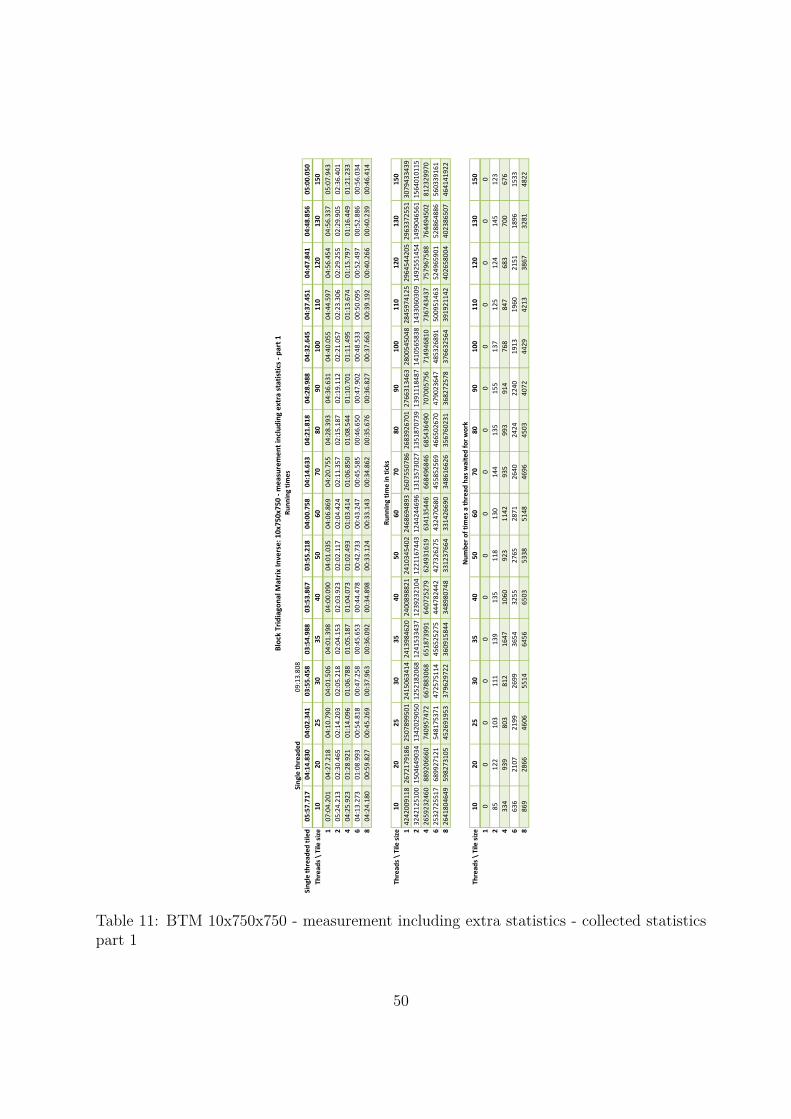
09:13.808

Sin

gle

th

read

ed

tile

d0

5:5

7.7

17

04

:14

.83

00

4:0

2.3

41

03

:55

.45

80

3:5

4.9

88

03

:53

.86

70

3:5

5.2

18

04

:00

.75

80

4:1

4.6

33

04

:21

.81

80

4:2

8.9

88

04

:32

.64

50

4:3

7.4

51

04

:47

.84

10

4:4

8.8

56

05

:00

.05

0

Thre

ads

\ Ti

le s

ize

10

20

25

30

35

40

50

60

70

80

90

10

01

10

12

01

30

15

0

107:04.201

04:27.218

04:10.790

04:01.506

04:01.398

04:00.090

04:01.035

04:06.869

04:20.755

04:28.393

04:36.631

04:40.055

04:44.597

04:56.454

04:56.337

05:07.943

205:24.213

02:30.465

02:14.203

02:05.218

02:04.153

02:03.923

02:02.117

02:04.424

02:11.357

02:15.187

02:19.112

02:21.057

02:23.306

02:29.255

02:29.905

02:36.401

404:25.923

01:28.921

01:14.096

01:06.788

01:05.187

01:04.073

01:02.493

01:03.414

01:06.850

01:08.544

01:10.701

01:11.495

01:13.674

01:15.797

01:16.449

01:21.233

604:13.273

01:08.993

00:54.818

00:47.258

00:45.653

00:44.478

00:42.733

00:43.247

00:45.585

00:46.650

00:47.902

00:48.533

00:50.095

00:52.497

00:52.886

00:56.034

804:24.180

00:59.827

00:45.269

00:37.963

00:36.092

00:34.898

00:33.124

00:33.143

00:34.862

00:35.676

00:36.827

00:37.663

00:39.192

00:40.266

00:40.239

00:46.414

Thre

ads

\ Ti

le s

ize

10

20

25

30

35

40

50

60

70

80

90

10

01

10

12

01

30

15

0

14242009118

2672179186

2507899501

2415063414

2413984620

2400898821

2410345402

2468694893

2607550786

2683926701

2766313463

2800545048

2845974125

2964544205

2963372551

3079433439

23242125100

1504649034

1342029050

1252182068

1241533437

1239232104

1221167443

1244244696

1313573027

1351870739

1391118487

1410565838

1433060309

1492551454

1499046561

1564010115

42659232460

889206660

740957472

667883068

651873991

640725279

624931619

634135446

668496846

685436490

707005756

714946810

736743437

757967588

764494502

812329970

62532725517

689927121

548175371

472575114

456525275

444782442

427326275

432470680

455852569

466502670

479023647

485326891

500951463

524965901

528864886

560339161

82641804649

598273105

452691953

379629722

360915844

348980748

331237664

331426690

348616626

356760231

368272578

376632564

391921142

402658004

402386507

464141922

Thre

ads

\ Ti

le s

ize

10

20

25

30

35

40

50

60

70

80

90

10

01

10

12

01

30

15

0

10

00

00

00

00

00

00

00

0

285

122

103

111

139

135

118

130

144

135

155

137

125

124

145

123

4334

939

803

812

1647

1060

923

1142

935

993

914

768

847

683

700

676

6636

2107

2199

2699

3654

3255

2765

2871

2640

2424

2240

1913

1960

2151

1896

1533

8869

2866

4606

5514

6456

6503

5338

5148

4696

4503

4072

4429

4213

3867

3281

4822

Blo

ck T

rid

iago

nal

Mat

rix

Inve

rse

: 1

0x7

50

x75

0 -

me

asu

rem

en

t in

clu

din

g e

xtra

sta

tist

ics

- p

art

1R

un

nin

g ti

me

s

Sin

gle

th

read

ed

Ru

nn

ing

tim

e in

tic

ks

Nu

mb

er

of

tim

es

a th

read

has

wai

ted

fo

r w

ork

Table 11: BTM 10x750x750 - measurement including extra statistics - collected statisticspart 1

50

Thre

ads

\ Ti

le s

ize

10

20

25

30

35

40

60

70

80

90

10

01

10

12

01

30

15

0

10

00

00

00

00

00

00

00

0

2304101

258042

972279

1422697

1612817

1997475

2025225

3538088

4203045

7095577

9846004

12894185

15678763

15351466

26235682

40282350

41124453

2123062

3088697

3682706

7742428

7039673

13483165

18405319

25587755

27583538

35688951

40570512

84361395

52863483

79745855

156380504

62617478

4230258

5587169

8157334

12067828

15573508

28989445

32250161

53029085

52893528

61873905

75183786

124317884

150494076

178426689

253332021

84278760

5605261

23809612

20341704

16597911

26540923

49974589

47685782

71257666

83869469

99103570

147212160

231551122

204795478

209853587

543283351

Thre

ads

\ Ti

le s

ize

10

20

25

30

35

40

50

60

70

80

90

10

01

10

12

01

30

15

0

128996761

4393868

2210942

1160685

924416

554032

318116

198969

132985

114561

86084

65050

48639

48269

35188

25543

2109338797

11826906

10980935

3295801

3138570

3419888

1952690

1784954

1475015

1004678

838166

846317

1079625

760706

742895

829705

4377234464

24741508

15132527

13271935

12147474

8561003

6979827

5978627

6362598

4467233

4979997

4151781

3612779

4119721

3369186

3471825

6799281171

43622460

39786969

17560152

16134436

15436618

12780984

15245762

8352171

8512016

7071339

5741215

7839001

7427045

8670213

6484582

81663980312

74271539

38847565

33912749

27899860

23509329

18871561

25938072

14399287

12920876

14864492

12033895

12786103

10186583

10991742

28021891

Thre

ads

\ Ti

le s

ize

10

20

25

30

35

40

50

60

70

80

90

10

01

10

12

01

30

15

0

114839408

1993082

997498

586508

404858

265184

134728

89732

56048

42938

32044

23162

16088

16088

10618

6548

214839408

1993082

997498

586508

404858

265184

134728

89732

56048

42938

32044

23162

16088

16088

10618

6548

414839408

1993082

997498

586508

404858

265184

134728

89732

56048

42938

32044

23162

16088

16088

10618

6548

614839408

1993082

997498

586508

404858

265184

134728

89732

56048

42938

32044

23162

16088

16088

10618

6548

814839408

1993082

997498

586508

404858

265184

134728

89732

56048

42938

32044

23162

16088

16088

10618

6548

Thre

ads

\ Ti

le s

ize

10

20

25

30

35

40

50

60

70

80

90

10

01

10

12

01

30

15

0

10

00

00

00

00

00

00

00

0

263

61

73

64

53

63

48

40

39

39

40

37

34

29

32

28

4247

257

309

309

294

271

346

264

224

264

278

261

221

256

201

263

6441

584

563

601

651

591

635

687

571

622

607

591

562

609

552

577

8660

1022

1191

1238

1079

1155

1279

1148

1125

1050

1071

1077

1050

1127

977

994

Nu

mb

er

of

tick

s a

thre

ad h

as w

aite

d f

or

wo

rk

Nu

mb

er

of

tick

s a

thre

ad h

as w

aite

d t

o e

nte

r Tr

yGe

tWo

rk m

eth

od

Nu

mb

er

of

tim

es

a th

read

has

co

mp

lete

d a

co

mp

uta

tio

nal

ke

rne

l

Nu

mb

er

of

tim

es

a th

read

has

re

ceiv

ed

wo

rk f

rom

a s

eco

nd

ary

pro

du

cer

(in

pip

elin

ed

mo

de

)

Blo

ck T

rid

iago

nal

Mat

rix

Inve

rse

: 1

0x7

50

x75

0 -

me

asu

rem

en

t in

clu

din

g e

xtra

sta

tist

ics

- p

art

2R

un

nin

g ti

me

s

Table 12: BTM 10x750x750 - measurement including extra statistics - collected statisticspart 2

51

Thre

ads

\ Ti

le s

ize

10

20

25

30

35

40

50

60

70

80

90

10

01

10

12

01

30

15

0

10.843

0.954

0.966

0.975

0.973

0.974

0.976

0.975

0.977

0.976

0.972

0.974

0.975

0.971

0.975

0.974

21.103

1.694

1.806

1.880

1.893

1.887

1.926

1.935

1.938

1.937

1.934

1.933

1.936

1.929

1.927

1.918

41.345

2.866

3.271

3.525

3.605

3.650

3.764

3.797

3.809

3.820

3.805

3.813

3.766

3.798

3.778

3.694

61.412

3.694

4.421

4.982

5.147

5.258

5.504

5.567

5.586

5.612

5.615

5.618

5.538

5.483

5.462

5.355

81.354

4.259

5.353

6.202

6.511

6.701

7.101

7.264

7.304

7.339

7.304

7.239

7.079

7.148

7.179

6.465

Thre

ads

\ Ti

le s

ize

10

20

25

30

35

40

50

60

70

80

90

10

01

10

12

01

30

15

0

10.000%

0.000%

0.000%

0.000%

0.000%

0.000%

0.000%

0.000%

0.000%

0.000%

0.000%

0.000%

0.000%

0.000%

0.000%

0.000%

20.005%

0.009%

0.036%

0.057%

0.065%

0.081%

0.083%

0.142%

0.160%

0.262%

0.354%

0.457%

0.547%

0.514%

0.875%

1.288%

40.011%

0.060%

0.104%

0.138%

0.297%

0.275%

0.539%

0.726%

0.957%

1.006%

1.262%

1.419%

2.863%

1.744%

2.608%

4.813%

60.017%

0.102%

0.170%

0.288%

0.441%

0.584%

1.131%

1.243%

1.939%

1.890%

2.153%

2.582%

4.136%

4.778%

5.623%

7.535%

80.020%

0.117%

0.657%

0.670%

0.575%

0.951%

1.886%

1.799%

2.555%

2.939%

3.364%

4.886%

7.385%

6.358%

6.519%

14.631%

Thre

ads

\ Ti

le s

ize

10

20

25

30

35

40

50

60

70

80

90

10

01

10

12

01

30

15

0

10.684%

0.164%

0.088%

0.048%

0.038%

0.023%

0.013%

0.008%

0.005%

0.004%

0.003%

0.002%

0.002%

0.002%

0.001%

0.001%

21.686%

0.393%

0.409%

0.132%

0.126%

0.138%

0.080%

0.072%

0.056%

0.037%

0.030%

0.030%

0.038%

0.025%

0.025%

0.027%

43.546%

0.696%

0.511%

0.497%

0.466%

0.334%

0.279%

0.236%

0.238%

0.163%

0.176%

0.145%

0.123%

0.136%

0.110%

0.107%

65.260%

1.054%

1.210%

0.619%

0.589%

0.578%

0.498%

0.588%

0.305%

0.304%

0.246%

0.197%

0.261%

0.236%

0.273%

0.193%

87.873%

1.552%

1.073%

1.117%

0.966%

0.842%

0.712%

0.978%

0.516%

0.453%

0.505%

0.399%

0.408%

0.316%

0.341%

0.755%

#Tile

s7

53

83

02

52

21

9#V

ALU

E!1

31

11

09

87

76

5

10.000%

0.000%

0.000%

0.000%

0.000%

0.000%

0.000%

0.000%

0.000%

0.000%

0.000%

0.000%

0.000%

0.000%

0.000%

0.000%

20.001%

0.006%

0.010%

0.019%

0.034%

0.051%

0.088%

0.145%

0.256%

0.313%

0.481%

0.588%

0.771%

0.765%

1.347%

1.844%

40.002%

0.047%

0.080%

0.138%

0.405%

0.398%

0.680%

1.257%

1.641%

2.260%

2.773%

3.209%

5.001%

4.073%

6.185%

9.358%

60.004%

0.106%

0.220%

0.458%

0.894%

1.213%

2.011%

3.100%

4.498%

5.344%

6.534%

7.629%

10.860%

11.793%

15.151%

18.970%

80.006%

0.144%

0.460%

0.931%

1.570%

2.394%

3.811%

5.426%

7.731%

9.492%

11.275%

16.052%

20.753%

19.379%

23.606%

42.410%

#Tile

s7

53

83

02

52

21

91

51

31

11

09

87

76

5

10.000%

0.000%

0.000%

0.000%

0.000%

0.000%

0.000%

0.000%

0.000%

0.000%

0.000%

0.000%

0.000%

0.000%

0.000%

0.000%

20.000%

0.003%

0.007%

0.011%

0.013%

0.024%

0.036%

0.045%

0.070%

0.091%

0.125%

0.160%

0.211%

0.180%

0.301%

0.428%

40.002%

0.013%

0.031%

0.053%

0.073%

0.102%

0.257%

0.294%

0.400%

0.615%

0.868%

1.127%

1.374%

1.591%

1.893%

4.016%

60.003%

0.029%

0.056%

0.102%

0.161%

0.223%

0.471%

0.766%

1.019%

1.449%

1.894%

2.552%

3.493%

3.785%

5.199%

8.812%

80.004%

0.051%

0.119%

0.211%

0.267%

0.436%

0.949%

1.279%

2.007%

2.445%

3.342%

4.650%

6.527%

7.005%

9.201%

15.180%

Blo

ck T

rid

iago

nal

Mat

rix

Inve

rse:

10

x75

0x7

50

- c

alcu

late

d s

tats

- m

eas

ure

me

nt

incl

ud

ing

ext

ra s

tati

stic

sSp

ee

du

p

% c

om

pu

tati

on

al k

ern

els

pip

elin

ed

= #

rece

ive

d w

ork

fro

m s

eco

nd

ary

pro

du

cer

/ #t

ota

l co

mp

uta

tio

nal

ke

rne

ls

% t

ime

s a

thre

ad a

ske

d in

vai

n f

or

wo

rk (

#wai

ted

fo

r w

ork

/ (

#wai

ted

fo

r w

ork

+ #

co

mp

uta

tio

nal

ke

rne

ls))

Spin

nin

g ti

me

in %

(#t

icks

sp

inn

ing/

(#th

read

s *

#to

tal t

icks

)

Wai

tin

g ti

me

in %

(#t

icks

wai

ted

/(#t

hre

ads

* #t

ota

l tic

ks)

Table 13: BTM 10x750x750 - measurement including extra statistics - calculated statistics

52

02:11.638

Sin

gle

thre

ade

d t

iled

01

:46

.02

30

1:1

7.0

99

01

:14

.39

50

1:1

3.1

97

01

:13

.64

30

1:1

3.6

91

01

:14

.71

40

1:1

8.2

54

01

:25

.01

90

1:2

7.1

79

01

:28

.44

30

1:2

9.6

63

01

:33

.71

00

1:4

0.5

89

01

:37

.58

10

1:4

8.7

11

Thre

ads

\ Ti

le s

ize

10

20

25

30

35

40

50

60

70

80

90

10

01

10

12

01

30

15

0

102:02.019

01:20.786

01:17.319

01:15.532

01:16.143

01:16.051

01:17.018

01:20.801

01:27.763

01:29.964

01:31.134

01:32.583

01:36.944

01:44.318

01:40.686

01:52.565

201:29.131

00:44.930

00:40.991

00:39.288

00:39.238

00:38.728

00:38.933

00:40.796

00:44.244

00:45.373

00:46.113

00:46.937

00:48.853

00:52.413

00:51.132

00:56.452

401:14.854

00:26.142

00:22.662

00:20.910

00:20.551

00:20.116

00:20.031

00:20.848

00:22.589

00:23.144

00:23.433

00:24.433

00:25.426

00:26.764

00:26.166

00:28.805

601:11.848

00:20.242

00:16.760

00:14.777

00:14.462

00:14.001

00:13.785

00:14.287

00:15.502

00:16.044

00:16.356

00:16.893

00:16.952

00:18.578

00:19.452

00:22.342

801:15.239

00:17.422

00:14.016

00:12.106

00:11.494

00:11.045

00:10.744

00:11.075

00:12.297

00:12.438

00:12.329

00:13.921

00:14.335

00:15.978

00:17.955

00:22.306

Thre

ads

\ Ti

le s

ize

10

20

25

30

35

40

50

60

70

80

90

10

01

10

12

01

30

15

0

10

00

00

00

00

00

00

00

0

286

112

107

139

157

131

111

145

132

103

124

118

90

101

100

46

4352

813

791

1174

1352

1204

847

761

714

663

553

662

613

479

426

312

6660

2031

2355

2947

2869

2662

2356

1983

1761

1966

1688

1469

1086

1529

2156

2707

8898

2972

4324

4738

4383

4452

4147

3502

4193

3775

3005

4659

4894

5630

6012

6922

Thre

ads

\ Ti

le s

ize

10

20

25

30

35

40

50

60

70

80

90

10

01

10

12

01

30

15

0

14470458

586508

307418

192668

134728

89732

42938

32044

23162

16088

10618

6548

6548

6548

3674

3674

24470458

586508

307418

192668

134728

89732

42938

32044

23162

16088

10618

6548

6548

6548

3674

3674

44470458

586508

307418

192668

134728

89732

42938

32044

23162

16088

10618

6548

6548

6548

3674

3674

64470458

586508

307418

192668

134728

89732

42938

32044

23162

16088

10618

6548

6548

6548

3674

3674

84470458

586508

307418

192668

134728

89732

42938

32044

23162

16088

10618

6548

6548

6548

3674

3674

Thre

ads

\ Ti

le s

ize

10

20

25

30

35

40

50

60

70

80

90

10

01

10

12

01

30

15

0

10

00

00

00

00

00

00

00

0

268

57

71

70

44

41

40

40

41

40

40

31

33

29

30

28

4461

340

305

226

303

265

289

274

275

264

238

266

255

259

252

247

6485

565

575

585

691

656

557

621

738

612

564

587

533

587

517

520

8719

1256

1343

1161

1146

1145

1222

1092

1216

1189

859

992

983

1170

518

487

Nu

mb

er

of

tim

es a

th

read

ha

s co

mp

lete

d a

co

mp

uta

tio

na

l ker

ne

l

Nu

mb

er

of

tim

es a

th

read

has

rec

eive

d w

ork

fro

m a

sec

on

dar

y p

rod

uce

r (i

n p

ipe

lined

mo

de

)

Blo

ck T

rid

iago

nal

Mat

rix

Inve

rse

: 10

x50

0x5

00

Ru

nn

ing

tim

es

Sin

gle

thre

ade

d

Nu

mb

er

of

tim

es a

th

read

has

wai

ted

fo

r w

ork

Table 14: BTM 10x500x500 - collected statistics

53

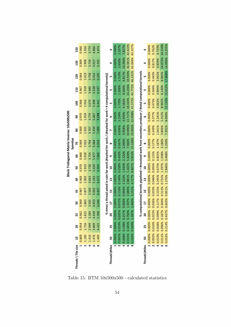
Thre

ads

\ T

ile s

ize

10

20

25

30

35

40

50

60

70

80

90

10

01

10

12

01

30

15

0

10.869

0.954

0.962

0.969

0.967

0.969

0.970

0.968

0.969

0.969

0.970

0.968

0.967

0.964

0.969

0.966

21.190

1.716

1.815

1.863

1.877

1.903

1.919

1.918

1.922

1.921

1.918

1.910

1.918

1.919

1.908

1.926

41.416

2.949

3.283

3.501

3.583

3.663

3.730

3.754

3.764

3.767

3.774

3.670

3.686

3.758

3.729

3.774

61.476

3.809

4.439

4.953

5.092

5.263

5.420

5.477

5.484

5.434

5.407

5.308

5.528

5.414

5.017

4.866

81.409

4.425

5.308

6.046

6.407

6.672

6.954

7.066

6.914

7.009

7.1

74

6.441

6.537

6.295

5.435

4.874

Thre

ads\

#til

es5

02

52

01

71

51

31

09

87

65

55

44

10.000%

0.000%

0.000%

0.000%

0.000%

0.000%

0.000%

0.000%

0.000%

0.000%

0.000%

0.000%

0.000%

0.000%

0.000%

0.000%

20.002%

0.019%

0.035%

0.072%

0.116%

0.146%

0.258%

0.450%

0.567%

0.636%

1.154%

1.770%

1.356%

1.519%

2.650%

1.237%

40.008%

0.138%

0.257%

0.606%

0.994%

1.324%

1.934%

2.320%

2.990%

3.958%

4.950%

9.182%

8.560%

6.817%

10.390%

7.827%

60.015%

0.345%

0.760%

1.507%

2.085%

2.881%

5.202%

5.828%

7.066%

10.890%

13.717%

18.324%

14.226%

18.930%

36.981%

42.423%

80.020%

0.504%

1.387%

2.400%

3.151%

4.727%

8.807%

9.852%

15.328%

19.005%

22.058%

41.572%

42.772%

46.231%

62.069%

65.327%

Thre

ads\

#til

es5

02

52

01

71

51

31

09

87

65

55

44

10.000%

0.000%

0.000%

0.000%

0.000%

0.000%

0.000%

0.000%

0.000%

0.000%

0.000%

0.000%

0.000%

0.000%

0.000%

0.000%

20.002%

0.010%

0.023%

0.036%

0.033%

0.046%

0.093%

0.125%

0.177%

0.249%

0.377%

0.473%

0.504%

0.443%

0.817%

0.762%

40.010%

0.058%

0.099%

0.117%

0.225%

0.295%

0.673%

0.855%

1.187%

1.641%

2.241%

4.062%

3.894%

3.955%

6.859%

6.723%

60.011%

0.096%

0.187%

0.304%

0.513%

0.731%

1.297%

1.938%

3.186%

3.804%

5.312%

8.965%

8.140%

8.965%

14.072%

14.154%

80.016%

0.214%

0.437%

0.603%

0.851%

1.276%

2.846%

3.408%

5.250%

7.391%

8.090%

15.150%

15.012%

17.868%

14.099%

13.255%

Spe

ed

up

% t

ime

s a

thre

ad a

sked

in v

ain

fo

r w

ork

(#w

aite

d f

or

wo

rk /

(#w

aite

d f

or

wo

rk +

# c

om

pu

tati

on

al k

ern

els)

)

% c

om

pu

tati

on

al k

ern

els

pip

elin

ed

= #

rece

ive

d w

ork

fro

m s

eco

nd

ary

pro

du

cer

/ #

tota

l co

mp

uta

tio

nal

ke

rnel

s

Blo

ck T

rid

iago

nal

Mat

rix

Inve

rse

: 1

0x5

00

x50

0

Table 15: BTM 10x500x500 - calculated statistics

54

00:28.844

Single threaded tiled 00:35.931 00:29.149 00:29.396 00:29.771 00:30.918 00:31.626 00:34.250 00:44.089

Threads\Tile size 10 20 25 30 35 40 50 80

1 00:43.680 00:31.897 00:31.840 00:31.900 00:33.021 00:33.721 00:36.410 00:46.363

2 00:35.409 00:18.323 00:17.631 00:17.022 00:17.342 00:17.571 00:18.838 00:24.085

4 00:26.509 00:11.111 00:10.029 00:09.522 00:09.524 00:09.584 00:10.479 00:17.260

6 00:25.370 00:09.206 00:07.976 00:07.392 00:07.370 00:07.616 00:08.986 00:16.276

8 00:26.789 00:08.468 00:07.175 00:06.617 00:06.876 00:07.263 00:08.793 00:16.295

Threads\Tile size 10 20 25 30 35 40 50 80

1 436796830 318965547 318398418 318998784 330213611 337207605 364104044 463627655

2 354086622 183232187 176305556 170217905 173422537 175714606 188383942 240852394

4 265093182 111112070 100293350 95222379 95238037 95835960 104789494 172596906

6 253699271 92058172 79759151 73922197 73698647 76159640 89857368 162761572

8 267890285 84684925 71747739 66170256 68758358 72627232 87929902 162954640

Threads\Tile size 10 20 25 30 35 40 50 80

1 0 0 0 0 0 0 0 0

2 905 1177 1045 939 705 676 514 727

4 2933 5976 5630 4719 4108 4816 6108 10653

6 3889 10498 10929 12351 14887 17764 24701 24810

8 5046 12377 17459 24215 32372 37131 42357 38680

Threads\Tile size 10 20 25 30 35 40 50 80

1 0 0 0 0 0 0 0 0

2 23317810 5589715 5225665 3808068 2998467 3732693 4613512 13488118

4 1716684 5741442 11679993 8607371 10753315 15155553 29291670 206661835

6 2892627 10223197 14162404 17698011 31680469 46029251 116931771 473141847

8 4329215 12533728 19059691 32792417 60858211 105644421 229119280 762393221

Threads\Tile size 10 20 25 30 35 40 50 80

1 2957673 536404 294542 192498 137273 96275 62235 30312

2 19496968 5985715 5218119 5282740 4644290 4083294 3762193 2386368

4 61590818 28487372 31422423 18627873 17088280 15421740 15800857 12183751

6 142140066 52803308 57247886 49187868 39221097 39435194 30711715 22858410

8 284279706 93711314 100592991 86512226 82683584 75223380 61247381 43159139

Threads\Tile size 10 20 25 30 35 40 50 80

1 1651403 252168 145990 92237 65228 45475 28427 11678

2 1651403 252168 145990 92237 65228 45475 28427 11678

4 1651403 252168 145990 92237 65228 45475 28427 11678

6 1651403 252168 145990 92237 65228 45475 28427 11678

8 1651403 252168 145990 92237 65228 45475 28427 11678

Threads\Tile size 10 20 25 30 35 40 50 80

1 0 0 0 0 0 0 0 0

2 714 530 490 488 434 451 445 361

4 2624 2938 2683 2704 2715 2537 2156 1246

6 4321 6178 6333 6064 5642 4655 3555 1392

8 5399 11036 11606 10162 8236 6699 3965 1417

Running times

Block Tridiagonal Matrix Inverse: 100x100x200 - measurement including extra statistics

Running time in ticks

Number of times a thread has waited for work

Number of ticks a thread has waited to enter TryGetWork method

Number of times a thread has completed a computational kernel

Number of times a thread has received work from a secondary producer (in pipelined mode)

Single threaded non tiled

Number of ticks a thread has waited for work

Table 16: BTM 100x100x200 - measurement including extra statistics - collected statistics.

55

Threads\Tile size 10 20 25 30 35 40 50 80

1 0.823 0.914 0.923 0.933 0.936 0.938 0.941 0.951

2 1.015 1.591 1.667 1.749 1.783 1.800 1.818 1.831

4 1.355 2.623 2.931 3.127 3.246 3.300 3.268 2.554

6 1.416 3.166 3.686 4.027 4.195 4.153 3.811 2.709

8 1.341 3.442 4.097 4.499 4.497 4.354 3.895 2.706

Threads\Tile size 10 20 25 30 35 40 50 80

1 0.0000% 0.0000% 0.0000% 0.0000% 0.0000% 0.0000% 0.0000% 0.0000%

2 3.2927% 1.5253% 1.4820% 1.1186% 0.8645% 1.0621% 1.2245% 2.8001%

4 0.1619% 1.2918% 2.9115% 2.2598% 2.8227% 3.9535% 6.9882% 29.9342%

6 0.1900% 1.8509% 2.9594% 3.9902% 7.1644% 10.0730% 21.6884% 48.4494%

8 0.2020% 1.8501% 3.3206% 6.1947% 11.0638% 18.1826% 32.5713% 58.4820%

Threads\Tile size 10 20 25 30 35 40 50 80

1 0.6771% 0.1682% 0.0925% 0.0603% 0.0416% 0.0286% 0.0171% 0.0065%

2 2.7531% 1.6334% 1.4799% 1.5518% 1.3390% 1.1619% 0.9985% 0.4954%

4 5.8084% 6.4096% 7.8326% 4.8906% 4.4857% 4.0230% 3.7697% 1.7648%

6 9.3378% 9.5598% 11.9627% 11.0900% 8.8697% 8.6299% 5.6964% 2.3407%

8 13.2647% 13.8323% 17.5255% 16.3427% 15.0316% 12.9468% 8.7068% 3.3107%

Threads\#tiles 15 8 6 5 5 4 3 2

1 0.0000% 0.0000% 0.0000% 0.0000% 0.0000% 0.0000% 0.0000% 0.0000%

2 0.0548% 0.4646% 0.7107% 1.0078% 1.0693% 1.4648% 1.7760% 5.8605%

4 0.1773% 2.3150% 3.7132% 4.8672% 5.9248% 9.5763% 17.6864% 47.7050%

6 0.2349% 3.9967% 6.9647% 11.8092% 18.5820% 28.0903% 46.4934% 67.9950%

8 0.3046% 4.6786% 10.6816% 20.7940% 33.1680% 44.9495% 59.8398% 76.8100%

Threads\#tiles 15 8 6 5 5 4 3 2

1 0.0000% 0.0000% 0.0000% 0.0000% 0.0000% 0.0000% 0.0000% 0.0000%

2 0.0432% 0.2102% 0.3356% 0.5291% 0.6654% 0.9918% 1.5654% 3.0913%

4 0.1589% 1.1651% 1.8378% 2.9316% 4.1623% 5.5789% 7.5843% 10.6696%

6 0.2617% 2.4500% 4.3380% 6.5744% 8.6497% 10.2364% 12.5057% 11.9198%

8 0.3269% 4.3764% 7.9499% 11.0173% 12.6265% 14.7312% 13.9480% 12.1339%

% computational kernels pipelined = #received work from secondary producer / #total computational

kernels

% times a thread asked in vain for work (#waited for work / (#waited for work + # computational

kernels))

Spinning time in % (#ticks spinning/(#threads * #total ticks)

Waiting time in % (#ticks waited/(#threads * #total ticks)

Speedup for 100x100x200 - measurement including extra statistics

Table 17: BTM 100x100x200 - measurement including extra statistics - calculated statistics

56

00:28.844

Single threaded tiled 00:35.931 00:29.149 00:29.396 00:29.771 00:30.918 00:31.626 00:34.250 00:44.089

Threads \ Tile size 10 20 25 30 35 40 50 80

1 00:43.429 00:31.784 00:31.788 00:31.836 00:33.008 00:33.769 00:36.375 00:46.351

2 00:33.037 00:18.446 00:17.729 00:16.969 00:17.398 00:17.635 00:18.805 00:24.173

4 00:26.486 00:11.161 00:10.124 00:09.527 00:09.531 00:09.607 00:10.477 00:17.273

6 00:25.338 00:09.133 00:08.072 00:07.384 00:07.387 00:07.608 00:08.978 00:16.252

8 00:26.868 00:08.435 00:07.230 00:06.597 00:06.802 00:07.527 00:08.809 00:16.364

Threads \ Tile size 10 20 25 30 35 40 50 80

1 0 0 0 0 0 0 0 0

2 927 1206 1052 927 697 680 517 723

4 3134 6163 5601 4702 4148 4830 6192 10753

6 4251 10689 11193 12513 15105 18311 24870 24932

8 5471 13204 17830 24653 32676 38343 42820 38784

Threads \ Tile size 10 20 25 30 35 40 50 80

1 1651403 252168 145990 92237 65228 45475 28427 11678

2 1651403 252168 145990 92237 65228 45475 28427 11678

4 1651403 252168 145990 92237 65228 45475 28427 11678

6 1651403 252168 145990 92237 65228 45475 28427 11678

8 1651403 252168 145990 92237 65228 45475 28427 11678

Threads \ Tile size 10 20 25 30 35 40 50 80

1 0 0 0 0 0 0 0 0

2 704 515 491 492 449 439 432 363

4 2588 2941 2697 2692 2699 2551 2181 1239

6 4771 6276 6374 6102 5629 4689 3593 1379

8 7576 11302 11803 10078 8385 6577 3888 1414

Threads \ #tiles 15 8 6 5 5 4 3 2

1 0.000% 0.000% 0.000% 0.000% 0.000% 0.000% 0.000% 0.000%

2 0.056% 0.476% 0.715% 0.995% 1.057% 1.473% 1.786% 5.830%

4 0.189% 2.386% 3.695% 4.850% 5.979% 9.601% 17.886% 47.938%

6 0.257% 4.066% 7.121% 11.946% 18.803% 28.707% 46.663% 68.102%

8 0.330% 4.976% 10.884% 21.091% 33.376% 45.746% 60.101% 76.858%

Threads \ #tiles 15 8 6 5 5 4 3 2

1 0.000% 0.000% 0.000% 0.000% 0.000% 0.000% 0.000% 0.000%

2 0.043% 0.204% 0.336% 0.533% 0.688% 0.965% 1.520% 3.108%

4 0.157% 1.166% 1.847% 2.919% 4.138% 5.610% 7.672% 10.610%

6 0.289% 2.489% 4.366% 6.616% 8.630% 10.311% 12.639% 11.809%

8 0.459% 4.482% 8.085% 10.926% 12.855% 14.463% 13.677% 12.108%

Threads \ Tile size 10 20 25 30 35 40 50 80

1 0.827 0.917 0.925 0.935 0.937 0.937 0.942 0.951

2 1.088 1.580 1.658 1.754 1.777 1.793 1.821 1.824

4 1.357 2.612 2.904 3.125 3.244 3.292 3.269 2.552

6 1.418 3.192 3.642 4.032 4.185 4.157 3.815 2.713

8 1.337 3.456 4.066 4.513 4.545 4.202 3.888 2.694

% computational kernels pipelined = #received work from secondary producer / #total

computational kernels

Single threaded non tiled

Speedup

% times a thread asked in vain for work (#waited for work / (#waited for work + #

computational kernels))

Block Tridiagonal Matrix Inverse: 100x100x200Running times

Number of times a thread has waited for work

Number of times a thread has completed a computational kernel

Number of times a thread has received work from a secondary producer (in pipelined

mode)

Table 18: BTM 100x100x200 - collected and calculated statistics

57

00:03.580

Single threaded tiled 00:05.130 00:04.654 00:04.836 00:05.089 00:05.262 00:05.750 00:06.248 00:08.925

Threads \ Tile size 10 20 25 30 35 40 50 80

1 00:06.655 00:05.480 00:05.711 00:05.810 00:05.943 00:06.434 00:06.893 00:09.493

2 00:05.726 00:03.486 00:03.353 00:03.391 00:03.450 00:03.804 00:04.350 00:07.449

4 00:03.934 00:02.596 00:02.388 00:02.506 00:02.680 00:02.857 00:03.404 00:06.165

6 00:03.722 00:02.368 00:02.383 00:02.537 00:02.672 00:02.966 00:03.673 00:06.363

8 00:04.204 00:02.688 00:02.665 00:02.754 00:03.095 00:03.276 00:03.956 00:06.659

Threads \ Tile size 10 20 25 30 35 40 50 80

1 0 0 0 0 0 0 0 0

2 980 654 469 476 487 589 907 1393

4 3114 3659 4600 6975 8490 9177 9539 5748

6 3825 9261 14913 17053 18500 19494 17493 10014

8 4166 16100 21558 23735 26030 27163 24250 13088

Threads \ Tile size 10 20 25 30 35 40 50 80

1 249083 46203 28834 19178 13634 11622 7383 3838

2 249083 46203 28834 19178 13634 11622 7383 3838

4 249083 46203 28834 19178 13634 11622 7383 3838

6 249083 46203 28834 19178 13634 11622 7383 3838

8 249083 46203 28834 19178 13634 11622 7383 3838

Threads \ Tile size 10 20 25 30 35 40 50 80

1 0 0 0 0 0 0 0 0

2 713 527 567 506 426 405 398 132

4 2694 2573 2205 1850 1380 1278 706 288

6 4822 5390 3818 2481 1676 1430 748 383

8 6405 7551 4019 2660 1741 1444 778 454

Threads \ #tiles 8 4 3 3 3 2 2 1

1 0.000% 0.000% 0.000% 0.000% 0.000% 0.000% 0.000% 0.000%

2 0.392% 1.396% 1.601% 2.422% 3.449% 4.824% 10.941% 26.630%

4 1.235% 7.338% 13.758% 26.670% 38.375% 44.122% 56.370% 59.962%

6 1.512% 16.697% 34.089% 47.067% 57.571% 62.649% 70.321% 72.293%

8 1.645% 25.841% 42.781% 55.310% 65.626% 70.035% 76.660% 77.325%

Threads \ #tiles 8 4 3 3 3 2 2 1

1 0.000% 0.000% 0.000% 0.000% 0.000% 0.000% 0.000% 0.000%

2 0.286% 1.141% 1.966% 2.638% 3.125% 3.485% 5.391% 3.439%

4 1.082% 5.569% 7.647% 9.646% 10.122% 10.996% 9.563% 7.504%

6 1.936% 11.666% 13.241% 12.937% 12.293% 12.304% 10.131% 9.979%

8 2.571% 16.343% 13.938% 13.870% 12.770% 12.425% 10.538% 11.829%

Threads \ Tile size 10 20 25 30 35 40 50 80

1 0.771 0.849 0.847 0.876 0.885 0.894 0.906 0.940

2 0.896 1.335 1.442 1.501 1.525 1.512 1.436 1.198

4 1.304 1.793 2.025 2.031 1.963 2.013 1.835 1.448

6 1.378 1.965 2.029 2.006 1.969 1.939 1.701 1.403

8 1.220 1.731 1.815 1.848 1.700 1.755 1.579 1.340

Speedup

Number of times a thread has received work from a secondary producer (in pipelined

mode)

Number of times a thread has completed a computational kernel

Number of times a thread has waited for work

Block Tridiagonal Matrix Inverse: 100x50x100Running times

Single threaded

% times a thread asked in vain for work (#waited for work / (#waited for work + #

computational kernels))

% computational kernels pipelined = #received work from secondary producer / #total

computational kernels

Table 19: BTM 100x50x100 - collected and calculated statistics

58

01:05.174

Single threaded tiled 01:20.381 01:03.626 01:02.792 01:02.916 01:04.203 01:05.476 01:09.813 01:26.184

Threads \ Tile size 10 20 25 30 35 40 50 80

1 01:34.607 01:07.534 01:06.342 01:06.060 01:07.404 01:09.196 01:13.347 01:30.349

2 01:10.393 00:38.385 00:36.193 00:35.096 00:35.206 00:35.757 00:37.670 00:46.128

4 00:58.738 00:22.911 00:20.393 00:19.132 00:18.932 00:19.145 00:19.823 00:28.090

6 00:55.554 00:18.505 00:15.785 00:14.288 00:13.990 00:14.023 00:14.711 00:25.014

8 00:58.329 00:16.875 00:13.674 00:12.059 00:11.728 00:11.753 00:13.309 00:24.353

Threads \ Tile size 10 20 25 30 35 40 50 80

1 0 0 0 0 0 0 0 0

2 951 1358 1348 1180 1074 941 693 545

4 3174 8174 7435 6373 5868 5168 4156 9780

6 4960 13554 14569 14382 13835 13736 17908 28221

8 5920 15534 20370 23481 26835 31794 45561 46373

Threads \ Tile size 10 20 25 30 35 40 50 80

1 3570840 531437 296253 186817 124708 89590 53670 18683

2 3570840 531437 296253 186817 124708 89590 53670 18683

4 3570840 531437 296253 186817 124708 89590 53670 18683

6 3570840 531437 296253 186817 124708 89590 53670 18683

8 3570840 531437 296253 186817 124708 89590 53670 18683

Threads \ Tile size 10 20 25 30 35 40 50 80

1 0 0 0 0 0 0 0 0

2 730 535 478 469 432 440 421 416

4 2485 2953 2829 2784 2738 2716 2639 1790

6 4651 6328 6471 6385 6207 6099 5385 2381

8 6224 11377 11796 11900 11381 10405 8078 2645

Threads \ #tiles 20 10 8 7 6 5 4 3

1 0.000% 0.000% 0.000% 0.000% 0.000% 0.000% 0.000% 0.000%

2 0.027% 0.255% 0.453% 0.628% 0.854% 1.039% 1.275% 2.834%

4 0.089% 1.515% 2.448% 3.299% 4.494% 5.454% 7.187% 34.360%

6 0.139% 2.487% 4.687% 7.148% 9.986% 13.294% 25.019% 60.168%

8 0.166% 2.840% 6.434% 11.166% 17.708% 26.193% 45.914% 71.282%

Threads \ #tiles 20 10 8 7 6 5 4 3

1 0.000% 0.000% 0.000% 0.000% 0.000% 0.000% 0.000% 0.000%

2 0.020% 0.101% 0.161% 0.251% 0.346% 0.491% 0.784% 2.227%

4 0.070% 0.556% 0.955% 1.490% 2.196% 3.032% 4.917% 9.581%

6 0.130% 1.191% 2.184% 3.418% 4.977% 6.808% 10.034% 12.744%

8 0.174% 2.141% 3.982% 6.370% 9.126% 11.614% 15.051% 14.157%

Threads \ Tile size 10 20 25 30 35 40 50 80

1 0.850 0.942 0.946 0.952 0.953 0.946 0.952 0.954

2 1.142 1.658 1.735 1.793 1.824 1.831 1.853 1.868

4 1.368 2.777 3.079 3.289 3.391 3.420 3.522 3.068

6 1.447 3.438 3.978 4.403 4.589 4.669 4.746 3.445

8 1.378 3.770 4.592 5.217 5.474 5.571 5.246 3.539

Block Tridiagonal Matrix Inverse: 100x150x250Running times

% times a thread asked in vain for work (#waited for work / (#waited for work + #

computational kernels))

% computational kernels pipelined = #received work from secondary producer / #total

computational kernels

Speedup

Single threaded

Number of times a thread has waited for work

Number of times a thread has completed a computational kernel

Number of times a thread has received work from a secondary producer (in pipelined

Table 20: BTM 100x150x250 - collected and calculated statistics

59

01:01.022

Single threaded tiled 01:17.464 01:03.200 01:02.677 01:03.449 01:05.466 01:06.956 01:11.692 01:33.501

Threads \ Tile size 10 20 25 30 35 40 50 80

1 01:32.749 01:07.685 01:07.170 01:07.336 01:09.692 01:11.420 01:16.030 01:38.308

2 01:13.440 00:38.841 00:37.338 00:36.016 00:36.918 00:37.233 00:39.304 00:51.107

4 00:57.117 00:24.226 00:21.564 00:20.204 00:20.276 00:20.414 00:21.848 00:36.057

6 00:54.501 00:19.784 00:17.366 00:15.693 00:15.578 00:16.115 00:18.588 00:33.771

8 00:57.565 00:18.286 00:15.523 00:14.096 00:14.220 00:15.195 00:18.224 00:33.936

Threads \ Tile size 10 20 25 30 35 40 50 80

1 0 0 0 0 0 0 0 0

2 1877 2461 2184 1922 1533 1380 1121 1390

4 6436 12934 11367 9896 8684 9540 11906 21617

6 8568 21403 23030 25510 29067 35532 48849 51184

8 10422 25705 36579 49136 64410 77364 85808 80608

Threads \ Tile size 10 20 25 30 35 40 50 80

1 3502566 543984 303448 196180 137217 96742 57702 24944

2 3502566 543984 303448 196180 137217 96742 57702 24944

4 3502566 543984 303448 196180 137217 96742 57702 24944

6 3502566 543984 303448 196180 137217 96742 57702 24944

8 3502566 543984 303448 196180 137217 96742 57702 24944

Threads \ Tile size 10 20 25 30 35 40 50 80

1 0 0 0 0 0 0 0 0

2 1470 1049 962 921 902 911 868 747

4 5193 5771 5338 5579 5408 5047 4271 2767

6 9555 12476 12626 12481 11382 9891 7155 3050

8 13157 22637 23719 21099 17272 14146 7893 3101

Threads \ #tiles 15 8 6 5 5 4 3 2

1 0.000% 0.000% 0.000% 0.000% 0.000% 0.000% 0.000% 0.000%

2 0.054% 0.450% 0.715% 0.970% 1.105% 1.406% 1.906% 5.278%

4 0.183% 2.322% 3.611% 4.802% 5.952% 8.976% 17.104% 46.427%

6 0.244% 3.786% 7.054% 11.507% 17.480% 26.862% 45.846% 67.234%

8 0.297% 4.512% 10.758% 20.030% 31.945% 44.435% 59.792% 76.368%

Threads \ #tiles 15 8 6 5 5 4 3 2

1 0.000% 0.000% 0.000% 0.000% 0.000% 0.000% 0.000% 0.000%

2 0.042% 0.193% 0.317% 0.469% 0.657% 0.942% 1.504% 2.995%

4 0.148% 1.061% 1.759% 2.844% 3.941% 5.217% 7.402% 11.093%

6 0.273% 2.293% 4.161% 6.362% 8.295% 10.224% 12.400% 12.227%

8 0.376% 4.161% 7.816% 10.755% 12.587% 14.622% 13.679% 12.432%

Threads \ Tile size 10 20 25 30 35 40 50 80

1 0.835 0.934 0.933 0.942 0.939 0.937 0.943 0.951

2 1.055 1.627 1.679 1.762 1.773 1.798 1.824 1.830

4 1.356 2.609 2.907 3.140 3.229 3.280 3.281 2.593

6 1.421 3.195 3.609 4.043 4.202 4.155 3.857 2.769

8 1.346 3.456 4.038 4.501 4.604 4.406 3.934 2.755

% times a thread asked in vain for work (#waited for work / (#waited for work + #

computational kernels))

% computational kernels pipelined = #received work from secondary producer / #total

computational kernels

Speedup

Block Tridiagonal Matrix Inverse: 200x100x200Running times

Single threaded

Number of times a thread has waited for work

Number of times a thread has completed a computational kernel

Number of times a thread has received work from a secondary producer (in pipelined

Table 21: BTM 200x100x200 - collected and calculated statistics

60

00:15.105

Single threaded tiled 00:18.724 00:15.308 00:15.325 00:15.569 00:16.029 00:16.541 00:17.885 00:23.361

Threads \ Tile size 10 20 25 30 35 40 50 80

1 00:22.315 00:17.124 00:16.970 00:17.567 00:17.386 00:17.822 00:19.075 00:24.551

2 00:15.313 00:10.257 00:09.391 00:11.141 00:09.420 00:09.316 00:10.018 00:12.770

4 00:11.751 00:06.374 00:05.784 00:06.950 00:05.264 00:05.274 00:05.534 00:09.079

6 00:11.067 00:05.189 00:04.754 00:05.692 00:04.160 00:04.277 00:04.725 00:08.510

8 00:11.690 00:04.896 00:04.334 00:05.535 00:03.850 00:03.885 00:04.636 00:08.649

Threads \ Tile size 10 20 25 30 35 40 50 80

1 0 0 0 0 0 0 0 0

2 473 624 557 467 364 318 247 341

4 1566 3246 2820 2364 2232 2375 2809 5284

6 2087 5501 5763 6317 7019 9079 12366 12794

8 2592 6827 8989 11955 16262 19139 22146 19390

Threads \ Tile size 10 20 25 30 35 40 50 80

1 868587 136561 75543 49493 33507 24185 14933 6194

2 868587 136561 75543 49493 33507 24185 14933 6194

4 868587 136561 75543 49493 33507 24185 14933 6194

6 868587 136561 75543 49493 33507 24185 14933 6194

8 868587 136561 75543 49493 33507 24185 14933 6194

Threads \ Tile size 10 20 25 30 35 40 50 80

1 0 0 0 0 0 0 0 0

2 366 257 230 239 239 252 222 197

4 1261 1438 1350 1341 1340 1246 1120 694

6 2286 3228 3148 3101 2802 2513 1851 794

8 2903 5794 5979 5216 4308 3676 2000 821

Threads \ #tiles 15 8 6 5 5 4 3 2

1 0.000% 0.000% 0.000% 0.000% 0.000% 0.000% 0.000% 0.000%

2 0.054% 0.455% 0.732% 0.935% 1.075% 1.298% 1.627% 5.218%

4 0.180% 2.322% 3.599% 4.559% 6.245% 8.942% 15.832% 46.036%

6 0.240% 3.872% 7.088% 11.319% 17.320% 27.294% 45.298% 67.379%

8 0.298% 4.761% 10.634% 19.455% 32.675% 44.176% 59.727% 75.790%

Threads \ #tiles 15 8 6 5 5 4 3 2

1 0.000% 0.000% 0.000% 0.000% 0.000% 0.000% 0.000% 0.000%

2 0.042% 0.188% 0.304% 0.483% 0.713% 1.042% 1.487% 3.180%

4 0.145% 1.053% 1.787% 2.709% 3.999% 5.152% 7.500% 11.204%

6 0.263% 2.364% 4.167% 6.266% 8.362% 10.391% 12.395% 12.819%

8 0.334% 4.243% 7.915% 10.539% 12.857% 15.200% 13.393% 13.255%

Threads \ Tile size 10 20 25 30 35 40 50 80

1 0.839 0.894 0.903 0.886 0.922 0.928 0.938 0.952

2 1.223 1.492 1.632 1.397 1.702 1.776 1.785 1.829

4 1.593 2.402 2.650 2.240 3.045 3.136 3.232 2.573

6 1.692 2.950 3.224 2.735 3.853 3.867 3.785 2.745

8 1.602 3.127 3.536 2.813 4.163 4.258 3.858 2.701

Speedup

Number of times a thread has received work from a secondary producer (in pipelined

Number of times a thread has completed a computational kernel

Number of times a thread has waited for work

Block Tridiagonal Matrix Inverse: 50x100x200Running times

Single threaded

% times a thread asked in vain for work (#waited for work / (#waited for work + #

computational kernels))

% computational kernels pipelined = #received work from secondary producer / #total

computational kernels

Table 22: BTM 50x100x200 - collected and calculated statistics

61

Single threaded non tiled:  02:24.780

Single threaded tiled 01:43.661 01:15.727 01:09.575 01:08.689 01:08.622 01:09.392 01:13.261 01:14.291 01:15.838 01:16.218 01:22.236

Threads \ Tile size 10 20 30 40 50 60 70 80 90 100 150

1 02:16.335 01:23.040 01:13.512 01:12.817 01:11.394 01:10.638 01:14.407 01:15.028 01:16.697 01:16.790 01:22.784

2 01:38.298 00:47.781 00:39.151 00:38.534 00:36.564 00:35.852 00:37.618 00:37.771 00:38.492 00:38.477 00:41.492

4 01:13.089 00:28.754 00:21.334 00:22.034 00:19.106 00:18.351 00:19.028 00:19.031 00:19.364 00:19.386 00:20.853

6 01:04.537 00:22.102 00:15.360 00:14.812 00:13.817 00:13.042 00:13.283 00:13.277 00:13.370 00:13.585 00:14.047

8 01:05.203 00:19.348 00:12.432 00:14.081 00:10.395 00:09.666 00:09.842 00:09.751 00:09.917 00:09.855 00:10.649

Threads \ Tile size 10 20 30 40 50 60 70 80 90 100 150

1 0 0 0 0 0 0 0 0 0 0 0

2 3 3 3 3 3 3 3 3 3 3 3

4 8 12 18 17 17 17 20 21 22 18 19

6 9 15 38 38 41 35 49 52 50 48 45

8 11 26 45 72 69 74 91 93 89 94 99

Threads \ Tile size 10 20 30 40 50 60 70 80 90 100 150

1 9045050 1136275 338350 143450 73810 42925 27434 19019 13685 9455 2870

2 9045050 1136275 338350 143450 73810 42925 27434 19019 13685 9455 2870

4 9045050 1136275 338350 143450 73810 42925 27434 19019 13685 9455 2870

6 9045050 1136275 338350 143450 73810 42925 27434 19019 13685 9455 2870

8 9045050 1136275 338350 143450 73810 42925 27434 19019 13685 9455 2870

Threads \ Tile size 10 20 30 40 50 60 70 80 90 100 150

1 0.000% 0.000% 0.000% 0.000% 0.000% 0.000% 0.000% 0.000% 0.000% 0.000% 0.000%

2 0.000% 0.000% 0.001% 0.002% 0.004% 0.007% 0.011% 0.016% 0.022% 0.032% 0.104%

4 0.000% 0.001% 0.005% 0.012% 0.023% 0.040% 0.073% 0.110% 0.161% 0.190% 0.658%

6 0.000% 0.001% 0.011% 0.026% 0.056% 0.081% 0.178% 0.273% 0.364% 0.505% 1.544%

8 0.000% 0.002% 0.013% 0.050% 0.093% 0.172% 0.331% 0.487% 0.646% 0.984% 3.334%

Threads \ Tile size 10 20 30 40 50 60 70 80 90 100 150

1 0.760 0.912 0.946 0.943 0.961 0.982 0.985 0.990 0.989 0.993 0.993

2 1.055 1.585 1.777 1.783 1.877 1.936 1.947 1.967 1.970 1.981 1.982

4 1.418 2.634 3.261 3.117 3.592 3.781 3.850 3.904 3.916 3.932 3.944

6 1 606 3 426 4 530 4 637 4 966 5 321 5 515 5 595 5 672 5 610 5 854

Number of times a thread has waited for work

Speedup

LU‐factorization: 3000x3000 matrixRunning times

% times a thread asked in vain for work (#waited for work / (#waited for work + # computational kernels))

Number of times a thread has completed a computational kernel

6 1.606 3.426 4.530 4.637 4.966 5.321 5.515 5.595 5.672 5.610 5.854

8 1.590 3.914 5.596 4.878 6.601 7.179 7.444 7.619 7.647 7.734 7.722

Table 23: LU-factorization: 3000x3000 - collected and calculated statistics

62

Single threaded non tiled:  08:38.534

Single threaded tiled 03:07.846 02:14.102 02:02.850 01:59.780 01:59.983 02:00.532 02:07.749 02:08.967 02:11.261 02:12.450 02:23.733

Threads \ Tile size 10 20 30 40 50 60 70 80 90 100 150

1 02:29.847 01:34.949 01:24.777 01:21.720 01:21.399 01:21.296 01:25.870 01:26.448 01:28.097 01:28.810 01:36.365

2 01:49.892 00:54.776 00:44.943 00:44.251 00:41.698 00:41.204 00:43.116 00:43.389 00:44.262 00:44.555 00:48.307

4 01:20.419 00:31.873 00:24.354 00:22.364 00:21.271 00:21.064 00:21.833 00:21.911 00:22.282 00:22.423 00:24.492

6 01:10.308 00:24.489 00:17.429 00:16.707 00:14.620 00:14.316 00:14.804 00:14.829 00:15.025 00:15.135 00:16.676

8 01:12.190 00:21.046 00:13.827 00:12.595 00:11.340 00:10.956 00:11.290 00:11.217 00:11.379 00:11.640 00:12.796

Threads \ Tile size 10 20 30 40 50 60 70 80 90 100 150

1 0 0 0 0 0 0 0 0 0 0 0

2 3 3 4 4 3 4 4 5 4 3 4

4 10 26 54 40 27 42 35 126 31 28 50

6 20 61 208 222 88 185 161 328 192 90 160

8 23 74 300 319 190 459 506 289 173 366 321

Threads \ Tile size 10 20 30 40 50 60 70 80 90 100 150

1 10479250 1317750 402220 170688 85850 51170 32412 22880 15428 11050 3570

2 10479250 1317750 402220 170688 85850 51170 32412 22880 15428 11050 3570

4 10479250 1317750 402220 170688 85850 51170 32412 22880 15428 11050 3570

6 10479250 1317750 402220 170688 85850 51170 32412 22880 15428 11050 3570

8 10479250 1317750 402220 170688 85850 51170 32412 22880 15428 11050 3570

Inverse: 2500x2500 matrixRunning times

Number of times a thread has waited for work

Number of times a thread has completed a computational kernel

% times a thread asked in vain for work (#waited for work / (#waited for work + # computational kernels))

Threads \ Tile size 10 20 30 40 50 60 70 80 90 100 150

1 0.000% 0.000% 0.000% 0.000% 0.000% 0.000% 0.000% 0.000% 0.000% 0.000% 0.000%

2 0.000% 0.000% 0.001% 0.002% 0.003% 0.008% 0.012% 0.022% 0.026% 0.027% 0.112%

4 0.000% 0.002% 0.013% 0.023% 0.031% 0.082% 0.108% 0.548% 0.201% 0.253% 1.381%

6 0.000% 0.005% 0.052% 0.130% 0.102% 0.360% 0.494% 1.413% 1.229% 0.808% 4.290%

8 0.000% 0.006% 0.075% 0.187% 0.221% 0.889% 1.537% 1.247% 1.109% 3.206% 8.250%

Threads \ Tile size 10 20 30 40 50 60 70 80 90 100 150

1 1.254 1.412 1.449 1.466 1.474 1.483 1.488 1.492 1.490 1.491 1.492

2 1.709 2.448 2.733 2.707 2.877 2.925 2.963 2.972 2.966 2.973 2.975

4 2.336 4.207 5.044 5.356 5.641 5.722 5.851 5.886 5.891 5.907 5.869

6 2.672 5.476 7.049 7.169 8.207 8.419 8.629 8.697 8.736 8.751 8.619

8 2.602 6.372 8.885 9.510 10.581 11.001 11.315 11.497 11.535 11.379 11.233

Threads \ Tile size 10 20 30 40 50 60 70 80 90 100 150

1 1.000 1.000 1.000 1.000 1.000 1.000 1.000 1.000 1.000 1.000 1.000

2 1.364 1.733 1.886 1.847 1.952 1.973 1.992 1.992 1.990 1.993 1.995

4 1.863 2.979 3.481 3.654 3.827 3.859 3.933 3.945 3.954 3.961 3.935

6 2.131 3.877 4.864 4.891 5.568 5.679 5.800 5.830 5.863 5.868 5.779

8 2.076 4.511 6.131 6.488 7.178 7.420 7.606 7.707 7.742 7.630 7.531

Speedup relative to 1 thread

Speedup

Table 24: Inverse: 2500x2500 - collected and calculated statistics

63

13:35.111

Single threaded tiled 04:31.700 03:06.800 02:46.100 02:41.700 02:40.300 02:40.900 02:48.400 02:50.200 02:52.000 02:53.000 03:04.600

Threads \ Tile size 10 20 30 40 50 60 70 80 90 100 150

1 03:48.649 02:19.881 02:05.970 02:02.404 02:00.583 02:00.544 02:06.090 02:07.014 02:08.584 02:09.520 02:17.737

2 02:39.952 01:21.536 01:06.562 01:02.993 01:00.773 01:00.642 01:03.222 01:03.723 01:04.440 01:04.840 01:09.074

4 02:01.768 00:48.250 00:36.084 00:36.453 00:31.903 00:31.149 00:32.054 00:32.120 00:32.417 00:32.592 00:34.880

6 01:47.283 00:37.039 00:25.863 00:25.837 00:21.589 00:21.249 00:21.651 00:21.665 00:21.841 00:21.935 00:23.423

8 01:49.384 00:31.868 00:20.914 00:21.623 00:17.064 00:16.295 00:16.500 00:16.457 00:16.545 00:16.748 00:17.965

Threads \ Tile size 10 20 30 40 50 60 70 80 90 100 150

1 0 0 0 0 0 0 0 0 0 0 0

2 3 4 4 4 4 4 4 5 4 3 4

4 9 24 55 37 25 39 41 140 36 24 49

6 18 57 180 172 96 187 198 344 213 108 96

8 27 100 375 425 203 526 537 611 180 443 291

Threads \ Tile size 10 20 30 40 50 60 70 80 90 100 150

1 15687500 1968750 599760 254016 127500 75852 47952 33792 22736 16250 5202

2 15687500 1968750 599760 254016 127500 75852 47952 33792 22736 16250 5202

4 15687500 1968750 599760 254016 127500 75852 47952 33792 22736 16250 5202

6 15687500 1968750 599760 254016 127500 75852 47952 33792 22736 16250 5202

8 15687500 1968750 599760 254016 127500 75852 47952 33792 22736 16250 5202

Single threaded non tiled: 

Minus ‐‐ Matrix ‐‐ Inverse‐Matrix Multiply: 2500x2500 matrixRunning times

Number of times a thread has waited for work

Number of times a thread has completed a computational kernel

% times a thread asked in vain for work (#waited for work / (#waited for work + # computational kernels))

Threads \ Tile size 10 20 30 40 50 60 70 80 90 100 150

1 0.000% 0.000% 0.000% 0.000% 0.000% 0.000% 0.000% 0.000% 0.000% 0.000% 0.000%

2 0.000% 0.000% 0.001% 0.002% 0.003% 0.005% 0.008% 0.015% 0.018% 0.018% 0.077%

4 0.000% 0.001% 0.009% 0.015% 0.020% 0.051% 0.085% 0.413% 0.158% 0.147% 0.933%

6 0.000% 0.003% 0.030% 0.068% 0.075% 0.246% 0.411% 1.008% 0.928% 0.660% 1.812%

8 0.000% 0.005% 0.062% 0.167% 0.159% 0.689% 1.107% 1.776% 0.785% 2.654% 5.298%

Threads \ Tile size 10 20 30 40 50 60 70 80 90 100 150

1 1.188 1.335 1.319 1.321 1.329 1.335 1.336 1.340 1.338 1.336 1.340

2 1.699 2.291 2.495 2.567 2.638 2.653 2.664 2.671 2.669 2.668 2.672

4 2.231 3.872 4.603 4.436 5.025 5.165 5.254 5.299 5.306 5.308 5.292

6 2.533 5.043 6.422 6.258 7.425 7.572 7.778 7.856 7.875 7.887 7.881

8 2.484 5.862 7.942 7.478 9.394 9.874 10.206 10.342 10.396 10.330 10.276

Threads \ Tile size 10 20 30 40 50 60 70 80 90 100 150

1 1.000 1.000 1.000 1.000 1.000 1.000 1.000 1.000 1.000 1.000 1.000

2 1.429 1.716 1.893 1.943 1.984 1.988 1.994 1.993 1.995 1.998 1.994

4 1.878 2.899 3.491 3.358 3.780 3.870 3.934 3.954 3.967 3.974 3.949

6 2.131 3.777 4.871 4.738 5.585 5.673 5.824 5.863 5.887 5.905 5.880

8 2.090 4.389 6.023 5.661 7.067 7.398 7.642 7.718 7.772 7.733 7.667

Speedup relative to 1 thread

Speedup

Table 25: Minus – Matrix – Inverse-Matrix Multiply: 2500x2500 - collected and calculatedstatistics

64

00:03.925

Single threaded tiled 00:05.500 00:01.900 00:01.100 00:01.500 00:00.900 00:01.000 00:00.800 00:00.800 00:00.800 00:00.800 00:00.800

10 20 30 40 50 60 70 80 90 100 150

1 00:02.802 00:01.673 00:01.336 00:01.226 00:01.078 00:01.085 00:00.819 00:00.728 00:00.729 00:00.705 00:00.768

2 00:02.419 00:01.489 00:01.260 00:00.971 00:00.548 00:00.506 00:00.457 00:00.572 00:00.702 00:00.545 00:00.592

4 00:02.282 00:00.814 00:00.501 00:01.052 00:01.005 00:00.780 00:00.678 00:00.403 00:00.400 00:00.377 00:00.383

6 00:02.025 00:00.885 00:00.575 00:00.589 00:00.496 00:01.574 00:01.248 00:00.714 00:00.815 00:02.026 00:03.321

8 00:14.704 00:08.145 00:02.890 00:18.513 00:07.635 00:06.193 00:01.216 00:04.165 00:00.942 00:00.639 00:07.579

Threads \ Tile size 10 20 30 40 50 60 70 80 90 100 150

1 0 0 0 0 0 0 0 0 0 0 0

2 0 0 0 0 0 0 0 0 0 0 0

4 0 0 0 0 0 0 0 0 0 0 0

6 0 0 0 0 0 0 0 0 0 0 0

8 0 0 0 0 0 0 0 0 0 0 0

Threads \ Tile size 10 20 30 40 50 60 70 80 90 100 150

1 250000 62500 27889 15625 10000 7056 5184 3969 3136 2500 1156

2 250000 62500 27889 15625 10000 7056 5184 3969 3136 2500 1156

4 250000 62500 27889 15625 10000 7056 5184 3969 3136 2500 1156

6 250000 62500 27889 15625 10000 7056 5184 3969 3136 2500 1156

8 250000 62500 27889 15625 10000 7056 5184 3969 3136 2500 1156

Threads \ Tile size 10 20 30 40 50 60 70 80 90 100 150

1 0.000% 0.000% 0.000% 0.000% 0.000% 0.000% 0.000% 0.000% 0.000% 0.000% 0.000%

2 0.000% 0.000% 0.000% 0.000% 0.000% 0.000% 0.000% 0.000% 0.000% 0.000% 0.000%

4 0.000% 0.000% 0.000% 0.000% 0.000% 0.000% 0.000% 0.000% 0.000% 0.000% 0.000%

6 0 000% 0 000% 0 000% 0 000% 0 000% 0 000% 0 000% 0 000% 0 000% 0 000% 0 000%

% times a thread asked in vain for work (#waited for work / (#waited for work + # computational kernels))

MinusPlusPlus: 5000x5000 matrixRunning times

Number of times a thread has completed a computational kernel

Number of times a thread has waited for work

Single threaded non tiled: 

6 0.000% 0.000% 0.000% 0.000% 0.000% 0.000% 0.000% 0.000% 0.000% 0.000% 0.000%

8 0.000% 0.000% 0.000% 0.000% 0.000% 0.000% 0.000% 0.000% 0.000% 0.000% 0.000%

Threads \ Tile size 10 20 30 40 50 60 70 80 90 100 150

1 1.963 1.136 0.823 1.223 0.835 0.922 0.977 1.099 1.097 1.135 1.042

2 2.274 1.276 0.873 1.545 1.642 1.976 1.751 1.399 1.140 1.468 1.351

4 2.410 2.334 2.196 1.426 0.896 1.282 1.180 1.985 2.000 2.122 2.089

6 2.716 2.147 1.913 2.547 1.815 0.635 0.641 1.120 0.982 0.395 0.241

8 0.374 0.233 0.381 0.081 0.118 0.161 0.658 0.192 0.849 1.252 0.106

Speedup

Table 26: MinusPlusPlus: 5000x5000 - collected and calculated statistics

65

04:56.007

Single threaded tiled 02:52.900 02:06.000 01:54.200 01:49.500 01:47.500 01:46.000 01:50.200 01:48.700 01:49.100 01:47.800 01:46.800

Threads \ Tile size 10 20 30 40 50 60 70 80 90 100 150

1 02:55.451 02:05.434 01:55.437 01:50.281 01:48.125 01:46.246 01:50.393 01:48.842 01:49.245 01:47.783 01:46.885

2 02:01.216 01:12.963 01:00.892 00:57.005 00:55.397 00:53.982 00:55.705 00:54.699 00:54.825 00:54.149 00:53.550

4 01:29.969 00:43.108 00:32.978 00:30.154 00:28.413 00:27.510 00:28.139 00:27.570 00:27.523 00:27.274 00:26.847

6 01:31.483 00:32.876 00:23.668 00:20.436 00:19.213 00:18.771 00:18.924 00:18.552 00:18.504 00:18.302 00:18.011

8 01:39.140 00:28.106 00:19.186 00:15.965 00:14.813 00:14.259 00:14.413 00:14.095 00:13.941 00:13.898 00:13.591

Threads \ Tile size 10 20 30 40 50 60 70 80 90 100 150

1 0 0 0 0 0 0 0 0 0 0 0

2 0 0 0 0 0 0 0 0 0 0 0

4 0 0 0 0 0 0 0 0 0 0 0

6 0 0 0 0 0 0 0 0 0 0 0

8 0 0 0 0 0 0 0 0 0 0 0

Threads \ Tile size 10 20 30 40 50 60 70 80 90 100 150

1 62500 15625 7056 3969 2500 1764 1296 1024 784 625 289

2 62500 15625 7056 3969 2500 1764 1296 1024 784 625 289

4 62500 15625 7056 3969 2500 1764 1296 1024 784 625 289

6 62500 15625 7056 3969 2500 1764 1296 1024 784 625 289

8 62500 15625 7056 3969 2500 1764 1296 1024 784 625 289

Threads \ Tile size 10 20 30 40 50 60 70 80 90 100 150

1 0.000% 0.000% 0.000% 0.000% 0.000% 0.000% 0.000% 0.000% 0.000% 0.000% 0.000%

2 0.000% 0.000% 0.000% 0.000% 0.000% 0.000% 0.000% 0.000% 0.000% 0.000% 0.000%

4 0.000% 0.000% 0.000% 0.000% 0.000% 0.000% 0.000% 0.000% 0.000% 0.000% 0.000%

6 0.000% 0.000% 0.000% 0.000% 0.000% 0.000% 0.000% 0.000% 0.000% 0.000% 0.000%

8 0.000% 0.000% 0.000% 0.000% 0.000% 0.000% 0.000% 0.000% 0.000% 0.000% 0.000%

Threads \ Tile size 10 20 30 40 50 60 70 80 90 100 150

1 0.985 1.005 0.989 0.993 0.994 0.998 0.998 0.999 0.999 1.000 0.999

2 1.426 1.727 1.875 1.921 1.941 1.964 1.978 1.987 1.990 1.991 1.994

4 1.922 2.923 3.463 3.631 3.783 3.853 3.916 3.943 3.964 3.952 3.978

6 1.890 3.833 4.825 5.358 5.595 5.647 5.823 5.859 5.896 5.890 5.930

8 1.744 4.483 5.952 6.859 7.257 7.434 7.646 7.712 7.826 7.757 7.858

Number of times a thread has waited for work

Number of times a thread has completed a computational kernel

% times a thread asked in vain for work (#waited for work / (#waited for work + # computational kernels))

Speedup

Multiply: 2500x2500 matrixRunning times

Single threaded non tiled: 

Table 27: Multiply: 2500x2500 - collected and calculated statistics

66

04:53.947

Single threaded tiled 02:56.276 02:06.550 01:54.113 01:49.166 01:47.437 01:45.900 01:50.199 01:48.668 01:49.113 01:47.722 01:46.783

Threads \ Tile size 10 20 30 40 50 60 70 80 90 100 150

1 02:56.258 02:05.783 01:55.586 01:50.872 01:48.585 01:46.801 01:50.434 01:48.892 01:49.085 01:47.794 01:46.643

2 02:04.356 01:12.673 01:00.871 00:56.793 00:55.448 00:54.213 00:55.721 00:54.749 00:54.885 00:54.249 00:53.628

4 01:31.534 00:43.715 00:33.269 00:31.121 00:28.851 00:27.786 00:28.211 00:27.696 00:27.615 00:27.297 00:26.898

6 01:33.945 00:33.725 00:23.748 00:23.333 00:19.766 00:18.895 00:19.068 00:18.579 00:18.607 00:18.354 00:18.053

8 01:41.400 00:28.703 00:19.306 00:17.179 00:15.314 00:14.527 00:14.507 00:14.085 00:14.029 00:13.969 00:13.624

Threads \ Tile size 10 20 30 40 50 60 70 80 90 100 150

1 0 0 0 0 0 0 0 0 0 0 0

2 0 0 0 0 0 0 0 0 0 0 0

4 0 0 0 0 0 0 0 0 0 0 0

6 0 0 0 0 0 0 0 0 0 0 0

8 0 0 0 0 0 0 0 0 0 0 0

Threads \ Tile size 10 20 30 40 50 60 70 80 90 100 150

1 62500 15625 7056 3969 2500 1764 1296 1024 784 625 289

2 62500 15625 7056 3969 2500 1764 1296 1024 784 625 289

4 62500 15625 7056 3969 2500 1764 1296 1024 784 625 289

6 62500 15625 7056 3969 2500 1764 1296 1024 784 625 289

8 62500 15625 7056 3969 2500 1764 1296 1024 784 625 289

Threads \ Tile size 10 20 30 40 50 60 70 80 90 100 150

1 0.000% 0.000% 0.000% 0.000% 0.000% 0.000% 0.000% 0.000% 0.000% 0.000% 0.000%

2 0.000% 0.000% 0.000% 0.000% 0.000% 0.000% 0.000% 0.000% 0.000% 0.000% 0.000%

4 0.000% 0.000% 0.000% 0.000% 0.000% 0.000% 0.000% 0.000% 0.000% 0.000% 0.000%

6 0.000% 0.000% 0.000% 0.000% 0.000% 0.000% 0.000% 0.000% 0.000% 0.000% 0.000%

8 0.000% 0.000% 0.000% 0.000% 0.000% 0.000% 0.000% 0.000% 0.000% 0.000% 0.000%

Threads \ Tile size 10 20 30 40 50 60 70 80 90 100 150

1 1.000 1.006 0.987 0.985 0.989 0.992 0.998 0.998 1.000 0.999 1.001

2 1.418 1.741 1.875 1.922 1.938 1.953 1.978 1.985 1.988 1.986 1.991

4 1.926 2.895 3.430 3.508 3.724 3.811 3.906 3.924 3.951 3.946 3.970

6 1.876 3.752 4.805 4.679 5.435 5.605 5.779 5.849 5.864 5.869 5.915

8 1.738 4.409 5.911 6.355 7.016 7.290 7.596 7.715 7.778 7.712 7.838

PlusMultiply: 2500x2500 matrixRunning times

Single threaded non tiled: 

% times a thread asked in vain for work (#waited for work / (#waited for work + # computational kernels))

Speedup

Number of times a thread has completed a computational kernel

Number of times a thread has waited for work

Table 28: PlusMultiply: 2500x2500 - collected and calculated statistics

67