1

Investigating Contextual Variability in Mode Choice: Accounting for Residential Neighborhood Type Choice

Liang Long* Cambridge Systematics Inc.

555 12th St. Suite 1600 Oakland, CA 94596

(510)873-8700 (phone) (510)873-8701(fax) Llong@camsys.com

Jie Lin

Department of Civil and Materials Engineering Institute of Environmental Science and Policy

University of Illinois at Chicago 842 W. Taylor St. (MC246)

Chicago, IL 60607 (312) 996-3068 (phone)

(312) 996-2426 (fax) janelin@uic.edu

Kimon Proussaloglou Cambridge Systematics Inc.

115 South Lasalle Street Chicago, IL 60603

(312)346-9907 (phone) (312)346-9908(fax)

Kproussaloglou@camsys.com

*Corresponding author

2

Abstract

In recent years, there have been increasing studies of understanding

the variability in travel behavior and advances in travel demand modeling

techniques have facilitated the variability study on mode choice.

In this paper a hierarchical random-coefficient mixed-logit model is

applied to quantify variability in household mode choice while accounting for

residential neighborhood types. A total of seven neighborhoods are defined in

the Chicago metropolitan area. The model accounts for the systematic and

random heterogeneity of individual mode choice and neighborhood type choice.

Individual level variables are extracted from a sample of 1300 households in

the study area. The contextual (defined by a census tract) variables are derived

from the Census Transportation Planning Package (CTPP) 2000.

It is found that individual mode choice behavior varies considerably

across different residential locations and there is a significant systematic and

random heterogeneity in the preference to transportation modes. Explicit

inclusion of contextual variability in the model improves the model estimation

power. Furthermore, background attributes affect mode choice through

modifying the marginal utilities associated with level of service, such as travel

time and travel cost.

The proposed methods of quantifying contextual variability in this

paper and the analysis findings will provide a useful tool for practitioners,

planners and policy makers in transportation analyses. Understanding the

influence of residential neighborhood type on travel behavior shed lights to

3

transportation decisions that involve the transportation-land use relationship,

increasing mobility and accessibility for communities, and coping with

changes of travel due to demographic change.

1. Introduction

Because of growing demand for high quality household travel data but

high costs associated with household surveys, transferability of household

travel survey data has recently gained increased attention. In fact,

transferability is not a new concept. Transportation model (and model

coefficient) transferability studies have been around for over four decades,

focusing on applying previously estimated mode choice and trip generation

model parameters to a new context (e.g., Badoe and Miller, 1995; Koppelman

and Wilmot, 1986, Karasmaa, 2001). In recent years, there have been several

studies of transferability of the 1995 Nationwide Person Travel Survey (NPTS)

and the 2001 National Household Travel Survey (NHTS) to local areas of

study (Wilmot and Stopher, 2001; Reuscher et al., 2001).

However, the contextual variability issue was not dealt with in the past

data transferability studies nor was it quantified. Contextual variability here

refers to the variability in travel behavior caused by contextual differences.

When considering data transferability from one context (one geographical area)

to another, it is naturally desirable that the contexts of the “lender” and the

“borrower” are homogeneous with regard to certain measures. The past studies

implicitly assumed that no behavioral variability was caused by the differences

between two areas and proceeded to transfer data from one area to the other. If

4

the transferred data were used for regional or local travel demand forecasting,

that assumption could lead to the potential danger of producing incorrect

model parameters even though the aggregate travel characteristics were

satisfactory.

Furthermore, there is a large body of literature to prove the impact of

the built environment on travel behavior(Ewing and Cervero, 2001; Rodriguez

and Joo, 2004; Handy et al., 2005; Cao et al., 2006; Krizek and Johnson, 2006;

Handy et al., 2006; Cao et al., 2007; Frank et al., 2007; Bhat and Guo, 2007).

Even intuitively, one would agree that members of a household living in New

York City may make very different travel decisions compared to those in a

household in Los Angeles, even if their socio-economic characteristics and

household structure are identical.

The objective of this paper is to quantify the mode choice contextual

variability in household travel pattern. That is, to answer the questions of what

the contextual effect really is on travel behavior and how much of the

behavioral variability can be attributed to contextual differences. It is of our

particular interest to quantify contextual variability in household mode choice

behavior in this paper.

A hierarchical random-coefficient mixed-logit model is proposed to

examine variability of state preference mode choice by extracting the census

and local survey data. The model is formulated in two levels. Individual

characteristics form the inputs to the first level of model, and the coefficients

of travel impedance (time and cost) is estimated by contextual attributes

5

including socio-demography, land use and journey-to-work attributes extracted

from the Census Tract Planning Package (CTPP) 2000.

Mixed-logit model are widely used in transportation demand analysis

(Srinivasan et al., 2006; Wang and Kockelman, 2006). Hierarchical mixed-

logit models in transportation analysis are relatively few. Bhat developed a

multi-level cross-classified work travel mode choice model to investigate

individual heterogeneity (micro level) and place heterogeneity (macro level)

for travel impedance (travel time and cost) instead of assuming the same travel

impedance to all the people within the same residence and work zones when

individuals make mode choice decisions (Bhat, 2000). On the other hand,

hierarchical models have been widely used in other fields like medicine and

epidemiology (e.g., Sullivan et al., 1999; Greenland, 2000; Burgess Jr. et al.,

2000), economics (e.g., Nunes Amaral et al., 1997; Goodman and Thibodeau,

1998), and educational, social, and behavioral sciences (e.g., Kreft, 1995;

Singer, 1998).

The rest of the paper is structured as follows. The data sources used in

this study are described in Section 2, followed by definition of neighborhood

types in Section 3. Section 4 presents the proposed hierarchical mixed-logit

model structure. This is followed by the model result discussion in Section 5.

Finally, several conclusions are drawn from the findings and the research

implications are discussed in Section 6.

6

2. Data Description

Two primary data sources are used in this study: (1) Pace (Suburban

Bus Service for Chicago Area) Survey data for Chicago area; (2) Census

Transportation Planning Package (CTPP) 2000. The analyses were conducted

using data fusion techniques and utilizing both local survey data and CTPP.

The two data sets were connected through a unique Census Tract identifier,

which provided an opportunity to understand contextual variability on travel

behavior.

The Pace Survey was designed and administered by MOREPACE

International Inc. between January and April 2006 for the Pace. The survey

collected commuters’ actual daily travel patterns, observed mode choice

behavior, attitudes toward everyday commuting and responses to a stated

choice experiment from 1,330 commuters in the six-county Chicago area (see

Cambridge Systematics Inc. report. for details on survey, sampling and

administration procedures). Chicago Area is chosen for study because they

have diverse travel modes and high usage of transit, which are not directly

explainable by their income level, occupation, and/or vehicle ownership, as

shown later in this session.

In this paper, we examine the state preference mode choice among five

motorized travel modes: Driving alone, Sharing a ride, Riding conventional

transit that currently is available, Riding the proposed Rapid Bus service; and

Using a vanpool service. The choice experiences focus on work travel and was

designed based on the real travel patterns that was provided in the recruit

7

survey. 1330 commuters were presented with three choice experiments and

three alternatives selected from the five modes based on available transit

options. Each option carried different characteristics (i.e., travel time, cost,

number of transfers) in each of the three choice experiments to determine the

conditions under which a respondent might change his or her mode of travel.

Another data source is Census Transportation Planning Package 2000.

Socioeconomic, demographic, land use and travel to work information in place

of residence provides the residential information at the census tract level.

3. Neighborhood Types

In previous work (Cambridge Systematics Inc., 2007), 1330 individuals

are divided into homogenous groups (we call them neighborhood types

hereafter) that share similar attitudes toward everyday travel. The purpose of

clustering is to reduce heterogeneity in analysis and then the contextual

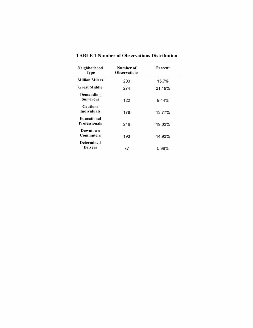
variability can be investigated within each neighborhood. Distribution of 1330

observations among seven segmentations is listed in Table 1.

Detailed methodology and description of each of seven clusters can be

found in Cambridge Systematics Inc. (2007). In short, these clusters refers to

distinct groups within the population that shared the same set of values.

Respondents’ attitudes towards their everyday travel experience were used to

reflect these values and identify a set of “homogeneous” segments that differed

as much as possible from the other segments. The features of the seven

neighborhoods are briefly summarized as follows.

8

1. Million Milers: mostly men, highly educated, live in larger households

with the highest percentage of two or more workers, lives and works

primarily in exurban and suburban areas. The predominant mode of travel

is by automobile (83 percent).

2. Great Middle: socioeconomic characteristics, home location, and

commuting patterns similar to Million Milers, high incomes, live and work

primarily in suburbs and exurbs, high automobile ownership, mostly use

their automobile to travel to work. However, they are more transit-oriented

and less automobile-friendly than Million Milers.

3. Demanding Survivors: Most members are women, live in small households,

lowest level of education and automobile ownership and a higher incidence

of incomes less than $35,000 per year, have varying commute patterns with

the second highest use of transit (48 percent), the highest usage of CTA rail

and Pace bus (10 and 19 percent, respectively), and the highest incidence

of reverse commute (15 percent of all work trips).

4. Cautious Individuals: share similar socioeconomic characteristics as

Demanding Survivors. Unlike the Demanding Survivors, three out of four

Cautious Individuals use their own car for their work commute. The travel

patterns in this group vary considerably with no single origin-destination

pattern emerging.

5. Educated Professionals: have the highest education level, live in large

households, mostly males, have at least two cars available, most members

reside in the suburbs, has the highest percentage of workers traveling to the

9

CBD (29 percent), automobile usage is the third lowest among the market

segments (58 percent) while transit usage is the third highest (39 percent).

6. Downtown Commuters: belonged primarily to high-income households,

the highest percentage of work locations in the Chicago CBD, highest

levels of Metra usage (36 percent), 11 percent of Pace usage.

7. Determined Drivers: strongly inclined towards using their own automobile

for commuting, mostly female commuters, live in, work in, and commute

between exurban and suburban locations, shows a very low market

penetration by transit, 95 percent automobile market share.

4. Hierarchical Model Structure

The general idea of quantifying contextual variability in household

travel involves developing statistical models that can be used to directly test

contextual variability in household travel. Household travel variability is

deemed to come from two sources in this study: the household itself and the

environment it is in. After controlling for the variation due to individual

household characteristics, the contextual variability that measures the variation

of household travel behavior due to contextual settings (e.g., the built

environment, neighborhood type, etc.) is investigated. The actual contextual

unit of analysis is defined by a census tract.

In a travel demand model (e.g., trip generation model or a mode choice

model), the household travel behavior – the dependent variable (e.g., number

of trips, modal split) – is formulated in two parts: a deterministic part as a

10

function of household (and mode specific) attributes and a random

measurement error:

(1)

In model (1), it is common practice to assume that the model

coefficients (β) are fixed across the entire region. That is, to assume that

households in the sub-regions share similar unit effects of the built

environment on β, even though in reality they could be quite different. The

random error term (ε) measures the individual deviation from the deterministic

estimate after household characteristics are taken into account.

To quantify geographical variability, model (1) is modified to include

contextual variables in the following way: i. model coefficients (β) are

hypothesized to vary by Census Tracts and to depend on the background

attributes; and ii. the measurement errors can be further decomposed to two

parts, i.e., errors due to random effects of contextual variability and individual

random white noise. Simply put, model (1) is modified to the following form:

(2)

where, is the census tract attribute matrix that produce systematic

heterogeneity in the means of the randomly distributed coefficients; is the

associated coefficient vector; and is the random effects due to unmeasured

area errors.

Thus, model (2) defines a hierarchical random coefficient model

structure. Specifically, it is a two-level random coefficient model. The lower

11

level contains individual households; the upper level contains the areas that the

households belong to.

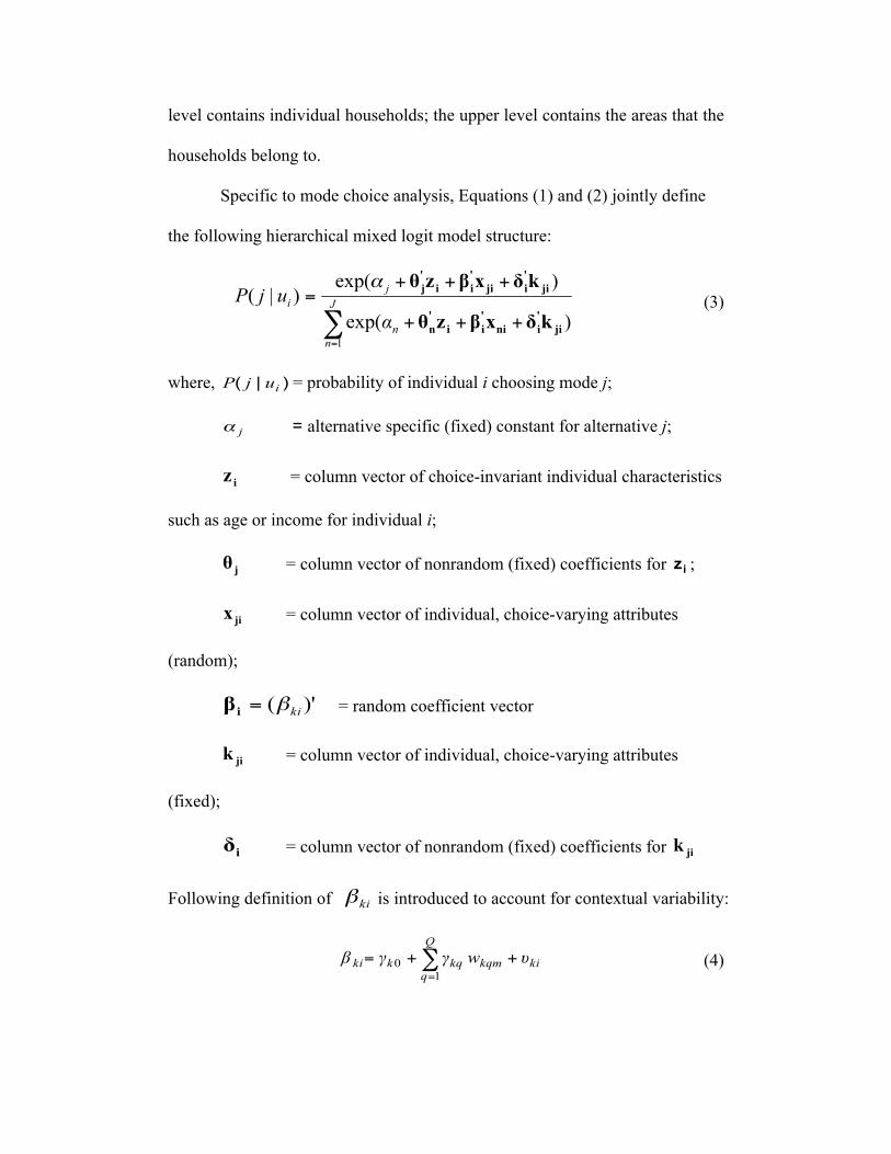
Specific to mode choice analysis, Equations (1) and (2) jointly define

the following hierarchical mixed logit model structure:

(3)

where, = probability of individual i choosing mode j;

= alternative specific (fixed) constant for alternative j;

= column vector of choice-invariant individual characteristics

such as age or income for individual i;

= column vector of nonrandom (fixed) coefficients for ;

= column vector of individual, choice-varying attributes

(random);

= random coefficient vector

= column vector of individual, choice-varying attributes

(fixed);

= column vector of nonrandom (fixed) coefficients for

Following definition of is introduced to account for contextual variability:

(4)

12

where, = qth weight for intercept (q=0) or neighborhood attribute

(q=1,2,…, Q)

= qth neighborhood (m =1,…, M) attribute associated with

coefficient , which produces an area specific mean.

= random effect associated with coefficient

The first term is a constant across neighborhoods. The middle terms

represent the extent to which the neighborhood attributes influence

, which is area specific heterogeneity. The last term defines the

random effect capturing the deviation (heterogeneity) from the average effect

of coefficient across individuals.

Mathematically speaking, the random coefficient are assumed

distributed randomly across individuals and the random parameters are allowed

to free correlation among each individuals. Triangle Distribution is assumed in

our model.

Combined with (4), Equation (3) can be re-written in the following:

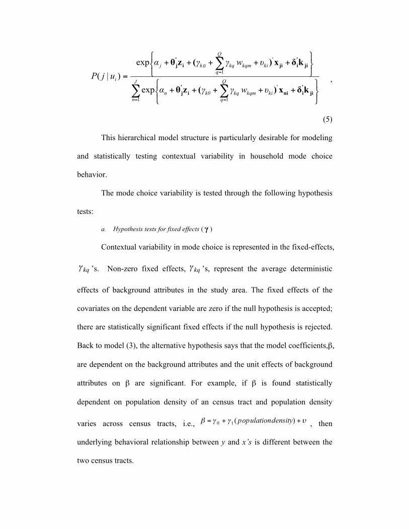
13

,

(5)

This hierarchical model structure is particularly desirable for modeling

and statistically testing contextual variability in household mode choice

behavior.

The mode choice variability is tested through the following hypothesis

tests:

a. Hypothesis tests for fixed effects ( )

Contextual variability in mode choice is represented in the fixed-effects,

’s. Non-zero fixed effects, ’s, represent the average deterministic

effects of background attributes in the study area. The fixed effects of the

covariates on the dependent variable are zero if the null hypothesis is accepted;

there are statistically significant fixed effects if the null hypothesis is rejected.

Back to model (3), the alternative hypothesis says that the model coefficients,β,

are dependent on the background attributes and the unit effects of background

attributes on β are significant. For example, if β is found statistically

dependent on population density of an census tract and population density

varies across census tracts, i.e., , then

underlying behavioral relationship between y and x’s is different between the

two census tracts.

14

b. Hypothesis tests for random effects ( )

Non-zero random effects, ’s, indicate deviations from the average

coefficients due to random variability in neighborhoods. Using the same

example as in the previous paragraph, even if the fixed effects ( ) are

statistically identical among the study areas, there still could be contextual

variability due to significant random effects ( ).

The fixed and random effects hypothesis tests combined, conclusions

can be made about the contextual variability in household travel across areas:

(i) if there are no significant fixed effects nor significant random effects, there

is no contextual effect on mode choice variability; (ii) if there are significant

fixed effects and no random effects, the area’s unit effects on household travel

are statistically identical and contextual variability can be ignored after the area

attributes are controlled for; and (iii) if the random effects are significant

(regardless of the fixed effects), there is significant contextual variability.

In order to test the neighborhood’s influence on the mode choice

behavior, alternative specific constant is defined to vary across

neighborhoods which are mentioned in the previous section. The null

hypothesis is of the form: H0: is equal among the neighborhoods for each

travel mode. That is, the travel mode shows different appeal to each

neighborhood if the null hypothesis is rejected. This further implies contextual

variability in mode choice behavior.

15

5. Model Results

Many neighborhood and household variables1 were tried and at the end

three neighborhood variables, percentage of retail workers in Manufacturing,

construction, maintenance or farming(referred as Percentage of retail workers

hereafter), percentage of White non-Hispanic American households and

Percentage of Industries in Professional, scientific, management,

administrative, and waste management services(referred as Percentage of

industries hereafter) are included in the model. Two household socio-

economic variables, (zero vehicle respondents and Female respondents), two

work location land use variables and a couple of level of service information

were statistically significant in the final model.

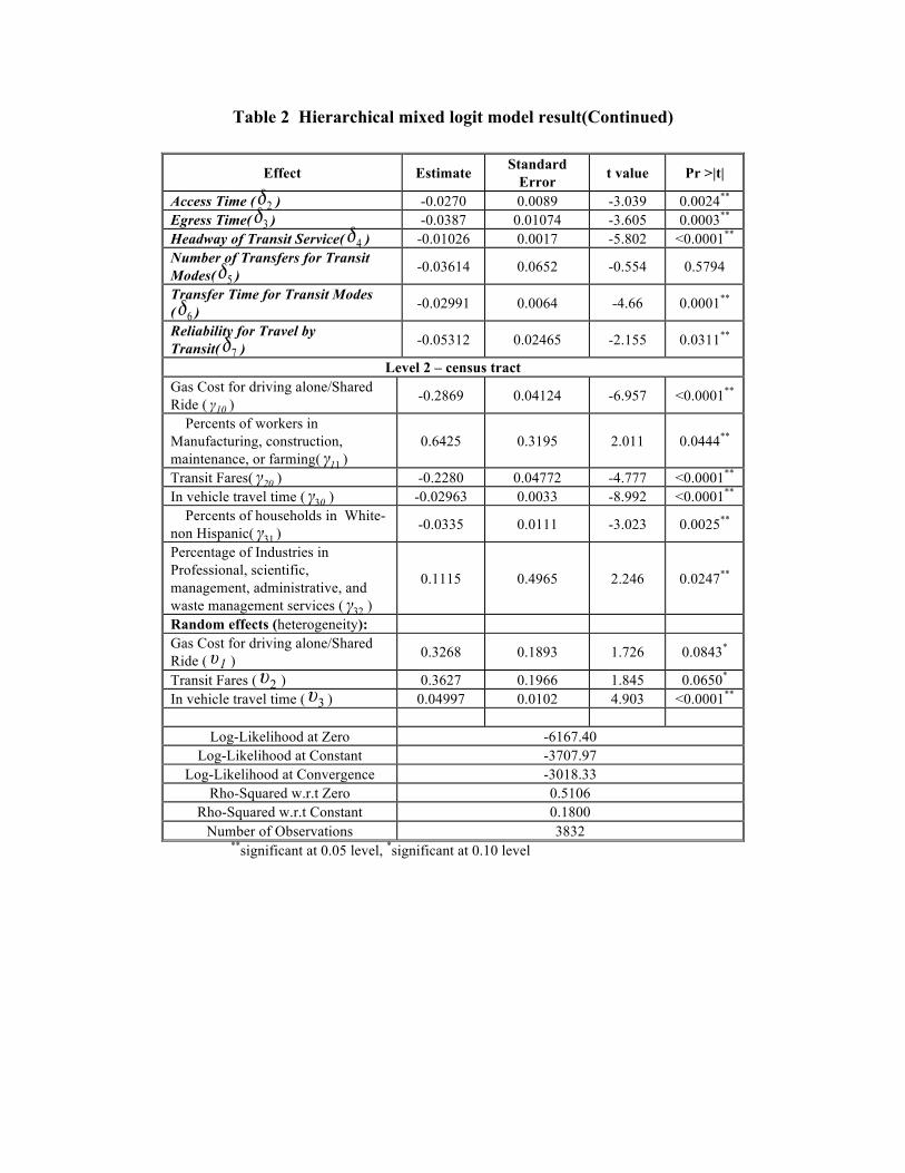
The final model specification and results are shown in Table 2. There

are a total of 3832 observations. The Log-likelihood at convergence is -

3018.33, whereas the log-likelihood values for the zero-coefficients and

constants-only models are -6167.40 and -3707.97, respectively. These explain

the reasonably high rho-squared value of 0.5106 with respect to (w.r.t.) zero

and 0.18 w.r.t constant and confirmed an overall good performance of the

model.

All the signs of the coefficients on the individual level (Level 1) are

intuitively correct. The constant for the drive alone mode is set to zero to serve

as a basis of comparison against the constants for the other four modes. The

constants for the share ride mode by cluster were all negative (-0.96 to -2.31)

and most were statistically significant. The constants for Great Middle, and

16

Cautious Individuals (Clusters 2 and 4) were larger in magnitude. This reflects

their difficulty of coordinating schedules while sharing a ride to work.

The overall constants for the existing transit modes were positive and

clearly suggests that existing transit service is perceived as competitive to the

automobile in cases where automobile and transit offer comparable levels of

service. This pattern is very reasonable in Chicago which is characterized by

prolonged congestion in the highway system and the high level of CBD-

oriented transit service.

Rapid Bus appears to be least appealing to Great Middles and Cautious

Individuals (Clusters 2 and 4). Members of these two market segments are

clearly more automobile-oriented in terms of their attitudes compared to all

other segments. Personal safety was a major concern for Cautious Individuals.

Therefore, the introduction of a new bus transit mode with a higher level of

service may not necessarily address the safety concerns of this particular group.

As a result, Rapid Bus may not appear as attractive to this segment relative to

other segments. In contrast, Rapid Bus is most appealing to Demand Survivors

and Downtown Commuters, reflecting transit-friendly attitudes of these market

segments, low automobile usage, and the comparatively high transit market

share, including Metra and Pace service.

The constant for the vanpool mode was negative and statistically

significant reflecting its much lower attractiveness when compared to the drive

alone option.

17

The alternative-specific zero vehicle respondents variables are positive

except for vanpool, indicating all else being equal an individual is more likely

to use other modes than to drive if the respondents don’t have vehicles. Among

the alternative-specific female respondents, the coefficients for existing transit

and BRT have significant negative signs, indicating that all else being equal

women are less likely to take transit than to drive.

The preference towards transit was highly dependent on the work

location. When the work destination is inside the Chicago CBD, transit

constants are increased by 1.34 and the transit is definitely perceived as the

preferred mode. Transit constants are lowered by 0.20 and 0.33 for existing

transit and BRT respectively when the destination is a suburban and the transit

is perceived less competitive compared with driving alone.

Most level of service coefficients at level one were strongly significant

and negative as expected.

In the Level 2 model specification, both gas cost ( ) and in vehicle

travel time ( ) have negatively significant coefficients at the 0.10 level. The

interaction term between individual gas cost and percentage of workers in

manufacturing, , is positive (0.6425) and statistically significant at the 0.05

level. This says that an individual whose marginal utility associated with gas

cost is positively affected by the percentage of workers in manufacturing in the

census tract the person lives in. In another word, people living in a

neighborhood of higher percentage of workers in manufacturing, construction,

maintenance or farming households are less sensitive to gas cost. The possible

18

explanation is people living in those census tracts are less likely to use

automobile and then gas costs tends to have less influence on them.

Percentage of White non-Hispanic households reduces the negative

marginal utility associated with in vehicle travel time for all modes considered.

This indicates that people living in a census tract of higher percentage of White

non-Hispanic are more sensitive to in vehicle travel time. Similarly, the

positive, significant interaction term between individual in vehicle travel time

and percentage of Industries in Professional, (-0.0335), indicates that an

individual’s marginal utility associated with in vehicle travel time is less

negative for all modes if his or her residential census tract has higher

percentage of industries in professional.

In both cases, the model results indicate that all other individual

measures being equal the same mode travel time or cost does not render the

same utility value as is generally assumed in mode choice analysis.

Interestingly, different from travel time and cost, transit fare tends not

to be affected by environmental factors. This is not hard to understand since

the transit fare are predetermined by the transit agencies and they should not be

correlated with census tract information.

The final fixed-effects portion of the model is shown in the following:

(6)

19

The ranges of and are [-0.189, 0.07] with an average of -

0.18(±0.059 - one standard deviation) and [-0.05, -0.006] with an average of -

0.04(±0.0.08), respectively. This variation is due to the differences in the two

background attributes across census tracts. Interestingly, the coefficient for Gas

Cost, , ranges from a negative -0.189 to a positive 0.07. This indicates that

in some households, increased gas cost actually resulted in increased utilities.

Further investigation reveals that among the households with a positive

value – there are only 6 such households, is within [0.02, 0.07] with a

standard deviation of 0.02, which indicates that for those households ,

although positive, is not statistically different from zero. In other words, gas

cost is an insignificant predictor of mode choice probability for those 6

households.

For the random effects, the estimate means the standard deviation from

the slope (β) of the same independent variable. If the estimate is statistically

significant, the associated random effect is significantly different from zero,

which means the total effect of the independent variable deviates statistically

from the fixed effects portion. The random effects of coefficients for travel

cost ( ), transit fare ( ) and travel time( ) are statistically significant,

suggesting that the deviations from the mean β’s (i.e., the fixed effects) are not

negligible across individuals living in the neighborhood.

[Table 2]

20

As another validity check, the expected value of time (VOT) from the

model equals , which is considered reasonable.

6. Concluding Remarks

In this paper, it has been showed that contextual variability in

individual mode choice can be formulated as a two-level random coefficient

modeling problem and thus can be tested statistically. The random coefficient

model structure is particularly desirable in studying the contextual effect of

built environments on travel behavior. By allowing both fixed and random

effects in the model coefficients, the model accounts for contextual variability

across geographic and allows incorporation of environmental covariates related

to neighborhood characteristics, which have been shown to have significant

influence on household travel.

The model shows significant effects of background attributes on mode

choice behavior. These findings confirm the effects of environmental factors

on household travel. It is found that individual mode choice behavior varies

considerably across different residential locations. Other than significant

systematic heterogeneity, there is significant random heterogeneity in the

preference to transportation modes.

This study has also quantified the neighborhood contextual effect on

mode choice. The contextual effect is through modifying the marginal utilities

associated with travel time and cost. In other words, the same person moving

between two different census tracts while keeping everything else the same

21

may have quite different mode choice utility values before and after, which are

likely to result in different mode choice probabilities.

Finally, it is important to recognize the limitations of this study. We

assembled a set of household and neighborhood variables available to us for

analysis. However, we do not intend to conclude that the assembled variables,

especially on the neighborhood level, have fully characterized the households

or the neighborhoods studied. Other unavailable measures, e.g., proximity to

highway/transit and more detailed land use categorization, will be of great

interest. This requires further research effort.

Notes:

1 A total of sixty-four neighborhood variables were extracted from the CTPP

2000 and were tried. All possible individual/household variables in the Pace

data set were also tried.

22

7. References

Badoe, A.D.and J. E. Miller (1995) Analysis of the Temporal Transferability

of Disaggregate Work Trip Mode Choice Model. Transportation Research

Record 1493:1-11, Transportation Research Board, National Research Council,

Washington D.C.

Bhat, C. R. and Guo, J. Y. (2007) A comprehensive analysis of built

environment characteristics on household residential choice and auto

ownership levels. Transportation Research Part B-Methodological, 41 (5),

506-526.

Bento, A.M., M.L. Cropper, A.M. Mobarak, K. Vinha (2005) The Effects of

Urban Spatial Structure on Travel Demand in The United States. The Review of

Economics and Statistics, 87(3): 466-478

Bhat, R.C. (2000) A Multi-Level Cross-Classified Model for Discrete

Response Variables. Transportation Research Part B, Vol. 34: 567-582

Burgess Jr., J.F., C.L. Christiansen, S.E. Michalak and C.N. Morris (2000)

Medical profiling: improving standards and risk adjustments using hierarchical

models. Journal of Health Economics, Volume 19, Issue 3: 291-309

Cambridge Systematics Inc. Pace Market Research Report, 2007.

23

Cao, X. Y., Mokhtarian, P. L. and Handy, S. L. (2006) Neighborhood design

and vehicle type choice: Evidence from Northern California. Transportation

Research Part D-Transport and Environment, 11 (2), 133-145.

Cao, X. Y., Mokhtarian, P. L. and Handy, S. L. (2007) Cross-sectional and

quasi-panel explorations of the connection between the built environment and

auto ownership. Environment and Planning A, 39 (4), 830-847.

Ewing, R. and Cervero, R. (2001) Travel and the Built Environment - A

Synthesis. Transportation Research Record, Journal of Transportation

Research Board (1780): 87-114 2001.

Frank, L., Kerr, J., Chapman, J. and Sallis, J. (2007) Urban form relationships

with walk trip frequency and distance among youth. American Journal of

Health Promotion, 21 (4), 305-311.

Giuliano, G., D. Narayan (2003) Another Look at Travel Patterns and Urban

Form: The US and Great Britain. Urban Studies, Vol. 40, No. 11: 2295-2312

Goodman, A.C. and T.G. Thibodeau (1998) Housing Market Segmentation.

Journal of Housing Economics, Volume 7, Issue 2: 121-143

Greenland, S. (2000b) Principles of multilevel modeling. International Journal

of Epidemiology 29: 158-167

Handy, S., Cao, X. Y. and Mokhtarian, P. (2005) Correlation or causality

between the built environment and travel behavior? Evidence from Northern

24

California. Transportation Research Part D-Transport and Environment, 10

(6), 427-444.

Handy, S., Cao, X. Y. and Mokhtarian, P. L. (2006) Self-selection in the

relationship between the built environment and walking - Empirical evidence

from northern California. Journal of the American Planning Association, 72

(1), 55-74.

Koppelman, F.S., and C.G. Wilmot (1986) The Effect of Omission of

Variables on Choice Model Transferability. Transportation Research, Part B:

Methodological, Vol. 20 B, No. 3: 205-213.

Karasmaa, N. (2001) The Spatial Transferability of the Helsinki Metropolitan

Area Mode Choice Models. Paper presented at the 5th workshop of the Nordic

Research Network on Modeling transport, Land-use and the Environment,

September 28-30, Nynashamn, Sweden

Kreft, I.G.G. (Ed.) (1995) Hierarchical linear models: problems and prospects

(special issue). Journal of Educational and Behavioral Statistics, 20(2)

Lin, J. and Long, L. (2008) “What Neighborhood Are You In? Empirical

Findings of Relationships between Household Travel and Neighborhood

Characteristics” Transportation, forthcoming

Nunes Amaral, L.A., S.V. Buldyrev, S. Havlin, P. Maass, M. A. Salinger, H.E.

Stanley and M.H.R. Stanley (1997) Scaling behavior in economics: The

25

problem of quantifying company growth. Physica A: Statistical and

Theoretical Physics, Volume 244, Issues 1-4: 1-24

Reuscher, T.R., R.L. Schmoyer. Jr., P.S. Hu (2001) Transferability of

Nationwide Personal Transportation Survey Data to Regional and Local Scales.

Transportation Research Record 1817: 25-32, Transportation Research Board,

National Research Council, Washington D.C.

Rodriguez, D. A. and Joo, J. (2004) The relationship between non-motorized

mode choice and the local physical environment. Transportation Research

Part D-Transport and Environment, 9 (2), 151-173.

Singer, J.D. (1998) Using SAS PROC MIXED to Fit Multilevel Models,

Hierarchical Models, and Individual Growth Models. Journal of Educational

and Behavioral Statistics, Vol. 24, No. 4: 323-355

Srinivasan, S., C.R. Bhat, J. Holguin-Veras (2006), An Empirical Analysis of

the Impact of Security Perception on Intercity Mode Choice Using a Panel

Rank-Ordered Mixed-Logit Model. Transportation Research Record 1942: 9-

15, Transportation Research Board, National Research Council, Washington

D.C.

Sullivan, L.M., K.A. Dukes, E. Losina (1999) Tutorial in Biostatistics An

Introduction to Hierarchical Linear Modelling. Statistics in Medicine 18: 855-

888

26

Timmermans, H., P. van der Waerden, M. Alves, J. Polak, S. Ellis, A. S.

Harvey, S. Kurose, R. Zandee (2003) Spatial context and the complexity of

daily travel patterns: an international comparison. Journal of Transport

Geography 11: 37-46

Wang, X and M.K Kockelman (2006) Tracking Land Cover Change in a

Mixed Logit Model: Recognizing Temporal and Spatial Effects.

Transportation Research Record 1977: 112-120, Transportation Research

Board, National Research Council, Washington D.C.

Wilmot, C.G. and P.R. Stopher (2001) Transferability of Transportation

Planning Data. Transportation Research Record 1768: 36-43, Transportation

Research Board, National Research Council, Washington D.C.

27

TABLE 1 Number of Observations Distribution

Neighborhood Type

Number of Observations

Percent

Million Milers 203 15.7% Great Middle 274 21.19% Demanding Survivors 122 9.44% Cautions

Individuals 178 13.77% Educational Professionals 246 19.03%

Downtown Commuters 193 14.93% Determined

Drivers 77 5.96%

28

Table 2 Hierarchical mixed logit model result

Effect Estimate Standard Error t value Pr >|t|

Level 1 - individual Intercept( ) Drive alone 0 Shared Ride -1.877 0.4695 -4.030 0.001**

Existing Transit 1.044 0.3178 3.285 0.001** BRT 0.8452 0.2665 3.170 0.0015** Vanpool -0.05122 0.3908 -0.131 0.8957 Intercept by clusters ( ) Drive alone 0 Shared Ride Clusters 3, 6 0 Clusters 1, 5, 7 0.9233 0.3495 2.642 0.0083** Clusters 2, 4 -0.3165 0.3306 -0.957 0.3385 Existing Transit Clusters 3, 6 0 Clusters 1, 5, 7 -0.4388 0.1568 -2.798 0.0051* Clusters 2, 4 -0.6511 0.1681 -3.874 0.0001** BRT Clusters 3, 6 0 Clusters 1, 5, 7 -0.5423 0.1362 -3.982 0.0001** Clusters 2, 4 -1.0178 0.1472 -6.914 <0.0001** Vanpool Clusters 3, 6 0 Clusters 1, 5, 7 -0.5981 0.2380 -2.513 0.0120** Clusters 2, 4 -0.8502 0.2417 -3.518 0.0004** Zero Vehicle respondents ( ) Drive along 0 Shared Ride 0.5526 0.6704 0.824 0.4098 Existing Transit 1.7287 0.5916 2.922 0.0035** BRT 1.4765 0.6017 2.454 0.0141** Vanpool -0.2137 1.5528 -0.138 0.8906 Female Respondents ( ) Drive along 0 Shared Ride 0.3201 0.2614 1.225 0.2207 Existing Transit -0.4629 0.1253 -3.692 0.0002** BRT -0.2439 0.1073 -2.272 0.0231** Vanpool -0.1693 0.1855 -0.913 0.3612 CBD Work Location ( ) Drive along 0 Existing Transit 1.3415 0.1782 7.592 <0.0001** BRT 0.9997 0.1753 5.702 <0.0001** Suburban Work Location ( ) Drive along 0 Existing Transit -0.2055 0.1458 -1.409 0.1587 BRT -0.3386 0.1159 -2.921 0.0035** Parking Cost for Drive alone/Shared Ride ( ) -0.00094 0.0020 -0.472 0.6372

29

Table 2 Hierarchical mixed logit model result(Continued)

Effect Estimate Standard Error t value Pr >|t|

Access Time ( ) -0.0270 0.0089 -3.039 0.0024** Egress Time( ) -0.0387 0.01074 -3.605 0.0003** Headway of Transit Service( ) -0.01026 0.0017 -5.802 <0.0001** Number of Transfers for Transit Modes( ) -0.03614 0.0652 -0.554 0.5794

Transfer Time for Transit Modes ( ) -0.02991 0.0064 -4.66 0.0001**

Reliability for Travel by Transit( ) -0.05312 0.02465 -2.155 0.0311**

Level 2 – census tract Gas Cost for driving alone/Shared Ride ( ) -0.2869 0.04124 -6.957 <0.0001**

Percents of workers in Manufacturing, construction, maintenance, or farming( )

0.6425 0.3195 2.011 0.0444**

Transit Fares( ) -0.2280 0.04772 -4.777 <0.0001** In vehicle travel time ( ) -0.02963 0.0033 -8.992 <0.0001** Percents of households in White-non Hispanic( ) -0.0335 0.0111 -3.023 0.0025**

Percentage of Industries in Professional, scientific, management, administrative, and waste management services ( )

0.1115 0.4965 2.246 0.0247**

Random effects (heterogeneity): Gas Cost for driving alone/Shared Ride ( ) 0.3268 0.1893 1.726 0.0843*

Transit Fares ( ) 0.3627 0.1966 1.845 0.0650* In vehicle travel time ( ) 0.04997 0.0102 4.903 <0.0001**

Log-Likelihood at Zero -6167.40 Log-Likelihood at Constant -3707.97

Log-Likelihood at Convergence -3018.33 Rho-Squared w.r.t Zero 0.5106

Rho-Squared w.r.t Constant 0.1800 Number of Observations 3832

**significant at 0.05 level, *significant at 0.10 level