investigating flat-slab subduction underneath south
TRANSCRIPT
INVESTIGATING FLAT-SLAB SUBDUCTION UNDERNEATH SOUTH AMERICA USING
4D NUMERICAL SIMULATIONS
BY
ARMANDO MIGUEL HERMOSILLO
THESIS
Submitted in partial fulfillment of the requirements
for the degree of Master of Science in Geology
in the Graduate College of the
University of Illinois at Urbana-Champaign, 2014
Urbana, Illinois
Advisor:
Professor Lijun Liu
ii
ABSTRACT
The Nazca Plate recycling underneath South America is an ideal example of
modern subduction, which provides an opportunity to study mechanisms of flat-slab
subduction and the nature of mantle seismic structures. Subduction occurring at this
location is characterized by along-trench variation from flat- to steep-dipping slabs, as
indicated by both seismic images and geological observations. First, we will
quantitatively investigate several earlier proposed conceptual mechanisms for flat-slab
subduction along the South American trench. Another target of this study is to better
understand the seismic structure under South America, where existing seismic imaging
results including studies of seismicity distribution and tomographic inversions still show
significant discrepancies. We therefore attempt to provide more constraints on the actual
mantle structure by comparing different seismic images with our 4D subduction model
predictions. We use forward data-assimilation models to simulate Nazca subduction
from 80 Ma to the present day. The models incorporate the age of the oceanic lithosphere,
kinematic plate motions through time, geometry of plate boundaries including that of the
South American trench, as well as thick cratons within the continent. Preliminary results
do show flat subduction and an overall match with present day tomography images
within the upper ~1000 km depth. However, the fit to mantle seismic images and slab
angle variation still need further improvements. Future models will progressively
assimilate more realistic subduction geometry including extended trench lines to the
north and over-thickened oceanic crust (oceanic plateaus or aseismic ridges) for a better
prediction of mantle structures.

iii
ACKNOWLEDGMENTS
First, I would like to thank and acknowledge my advisor Lijun Liu for all of his help and support
throughout my time as a graduate student. I only spent one year in Lijun’s group, and I learned
an exceptional amount about geodynamics in general and subduction simulation in particular.
Lijun has been providing thorough advises and assistance on every aspect of my research. I feel
fortunate that within such a short time period, we had work out a functioning model for South
American subduction, which, with many complexities both in geology and numerical simulation,
represents a good step forward in understanding abnormal subduction processes on Earth.
Second, I owe my thanks to Professor Craig Lundstrom, who spent time editing and providing
helpful suggestions for my thesis.
I would also like to thank the members of my research group. Jiashun Hu has been working
closely with me on constructing the South American subduction model, and I appreciate his help
with generating seismic tomography images to be compared with my subduction model results. I
also thank Tiffany Leonard and Quan Zhou for putting their work on halt to assist me whenever I
needed help.
Finally, I want to thank my family and friends for their love and support.
Without all the help I received, this project would not have been possible.
iv
TABLE OF CONTENTS
Chapter 1: Introduction ................................................................................................................................ 1
Chapter 2: Model Set-up ............................................................................................................................... 4
Chapter 3: Preliminary Results.................................................................................................................... 14
Chapter 4: Conclusion and Future Work ..................................................................................................... 28
References .................................................................................................................................................. 29
1
CHAPTER 1
INTRODUCTION
The western margin of South America has long been an active research area for subduction
dynamics. On the one hand, it has been difficult to determine what controls the abnormal
subduction processes seen along the South American trench. On the other hand, it is not entirely
clear how past subduction relates to the present seismic structures seen through seismic
tomographic inversions. Many attribute the upper mantle tomography structure (e.g., Grand, 2002)
to the varying angle of subduction along the western margin (e.g., Gutscher et al., 2000), but these
seismic images provide a mixed fit to the orientation of Benioff zones (Hayes et al., 2012),
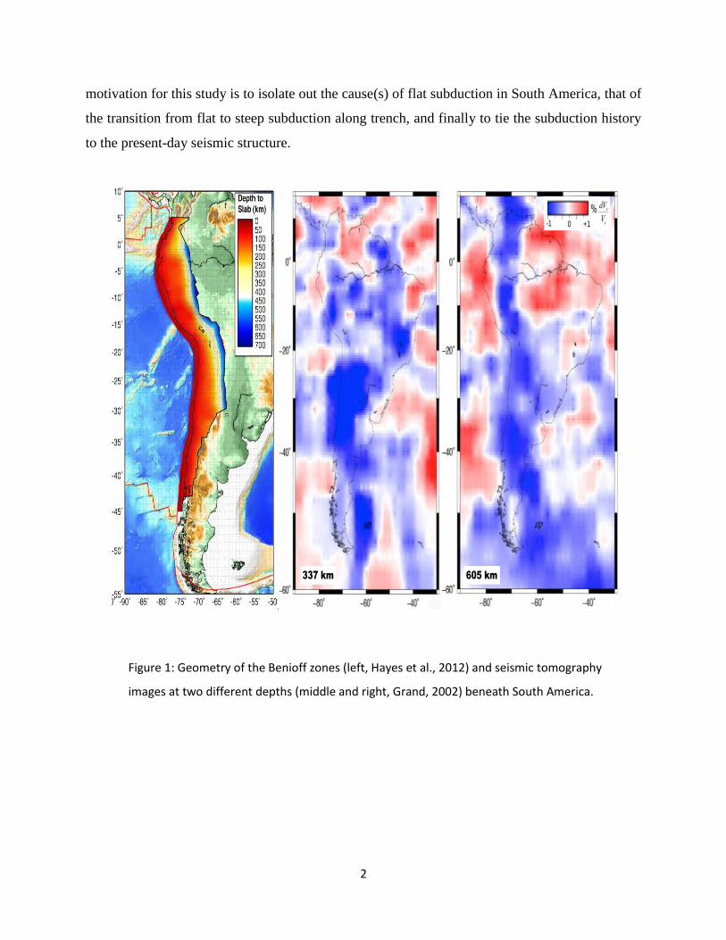
especially at shallow depths (Figure 1). Specifically, in this study, the Nazca and South American
plate interface is modeled to help shed some light on this issue. Subduction dip angle varies in the
north-south direction, from usual steep subduction (angle ≥30̊) between 10 °S and 25 °S to flat
subduction (angle <30̊) further north in Peru and south in Chile (Figure 1), as revealed by present-
day seismicity distributions (Hayes et al., 2012). However, it is unlikely that the current slab
geometry would have remained the same during the geological past, and its relation to deeper
mantle structures, therefore, remains unclear. For an example, global tomography outlines
voluminous fast seismic anomalies at lower mantle depths beneath the southern end of South
America, and their positions are not well connected with present day subduction (Ritsema et al.,
1999; Grand, 2002).
Flat subduction is occurring along 10% of present-day convergent boundaries (Hayes et
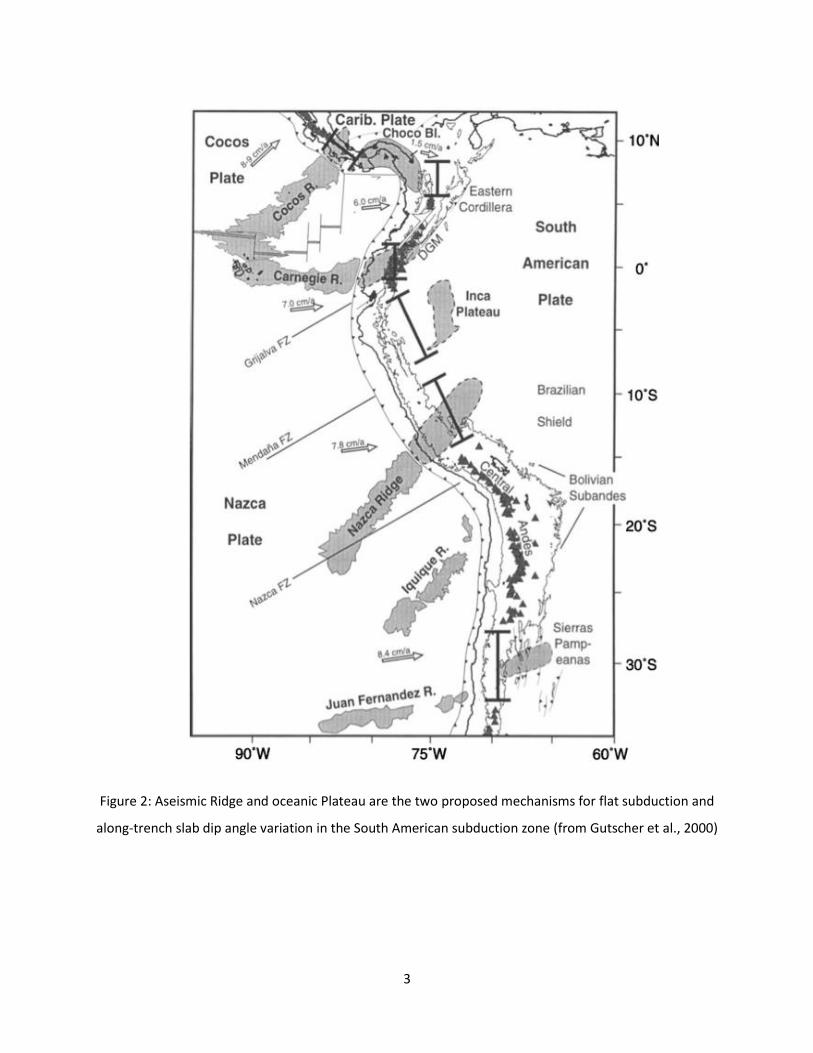
al., 2012) and many hypotheses have been proposed for its formation underneath South America
(Figure 2). Five potential causes for flat subduction have been suggested and are listed as follows:
Interplate hydrodynamic suction (Stevenson and Turner, 1977; Manea et al., 2012), subduction of
young and buoyant lithosphere (van Hunen et al., 2004), subduction of over-thickened oceanic
crust (Gerya et al., 2009), curvature of the margin (Gutscher et al., 2000), and the rapid absolute
motion of the overriding plate (Coney & Reynolds, 1977). Although a combination of these
components will more likely explain flat subduction than any individual one, it seems that over-
thickened crust is the most widely accepted hypothesis (Gutscher et al., 1999; 2000; van Hunen et
al., 2004; Liu et al., 2010). This seems to be the case for South America as well (Figure 2). The
2
motivation for this study is to isolate out the cause(s) of flat subduction in South America, that of
the transition from flat to steep subduction along trench, and finally to tie the subduction history
to the present-day seismic structure.
Figure 1: Geometry of the Benioff zones (left, Hayes et al., 2012) and seismic tomography
images at two different depths (middle and right, Grand, 2002) beneath South America.
-1 +10
dVs
Vs
605 km337 km
3
Figure 2: Aseismic Ridge and oceanic Plateau are the two proposed mechanisms for flat subduction and
along-trench slab dip angle variation in the South American subduction zone (from Gutscher et al., 2000)
4
CHAPTER 2
MODEL SET-UP
2.1 Work plan
We perform forward subduction models that run from 80 million years ago (Ma) to
the present day, which represents enough time to establish a subduction system comparable
to the observed mantle seismic structure. The models are constrained by various
observational records including paleo-seafloor ages, a continuous plate motion history, and
temporally evolving plate boundaries (Muller et al., 2008). In evaluating the mechanisms
of flat subduction formation, this standard model setup naturally incorporates all of the
above-mentioned components except for over-thickened crust. This factor is left out in
order to evaluate if it is required for flat subduction to occur along western South America.
All mechanisms except that of the thick crust can be realized in the subduction model. For
example:
1) To evaluate the hydrodynamic suction hypothesis, we incorporate the South
America cratons as thicker-than-ambient lithosphere patches (Gung et al., 2003).
The hydrodynamic suction force is a function of viscosity contrast between the
asthenosphere and lithosphere as well as of the position of the thick cratonic root
(e.g., Manea et al., 2012). Geometry and position of these cratons are prescribed as
high-viscosity structures inside the overriding plate, and are assimilated into the
model at each time step during the simulation run. In practice, we can turn these
features on and off to quantify the effects of craton-induced suction forces.
2) On the effect of trench curvature, our model assimilates the South American trench
plotted in the present-day coordinates, where trench migration from 81 Ma to the
present is shown (Figure 4). The positions in the past are rotated trench files from
the present-day geometry using the finite rotation poles of South America.
Intuitively, a straight trench line should produce linear slab features at depth. The
incorporation of a natural trench allows us to examine the effect of trench curvature
on slab morphology. Today we see that steep subduction happens at 10°S -25 °S,
5
where the subduction zone forms a concave shape, and shallow to flat subduction
further north with a convex shape in trench geometry (Figure 1). It is unknown,
however, whether this actually plays a role in the variation or if it is just a
coincidence.
3) South American plate has been moving westward since Late Cretaceous, and it is
suggested that this rapid overriding plate motion may lead to obduction (van Hunen
et al., 2004). Obduction is when the overriding plate moves so fast that it grinds on
top of an oceanic plate and does not allow it to subduct normally, as shown by 2D
numerical simulations (van Hunen et al., 2004). In our model, the velocity fields
are based on a recent plate reconstruction (Muller et al., 2008), and these fields are
generated through the GPlates software package using a CitcomS finite element
mesh (Gurnis et al., 2012). In practice, we can also vary the overriding plate speed
following different plate reconstructions to fully examine its impact on subducting
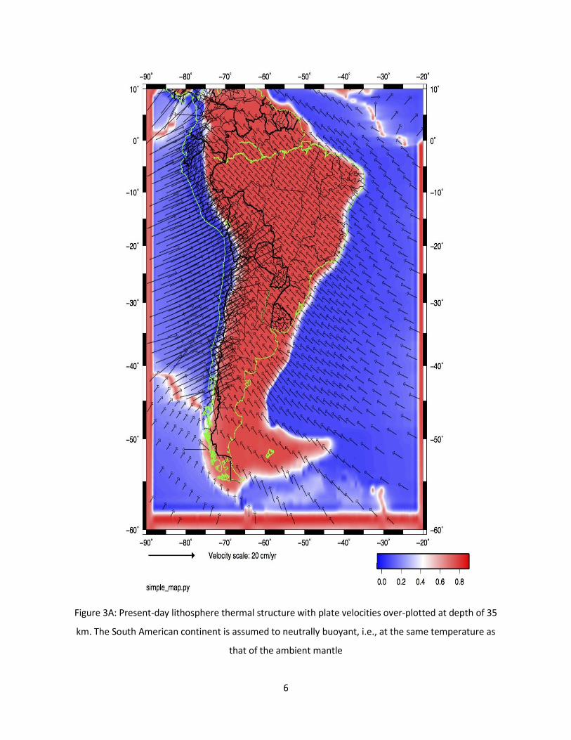
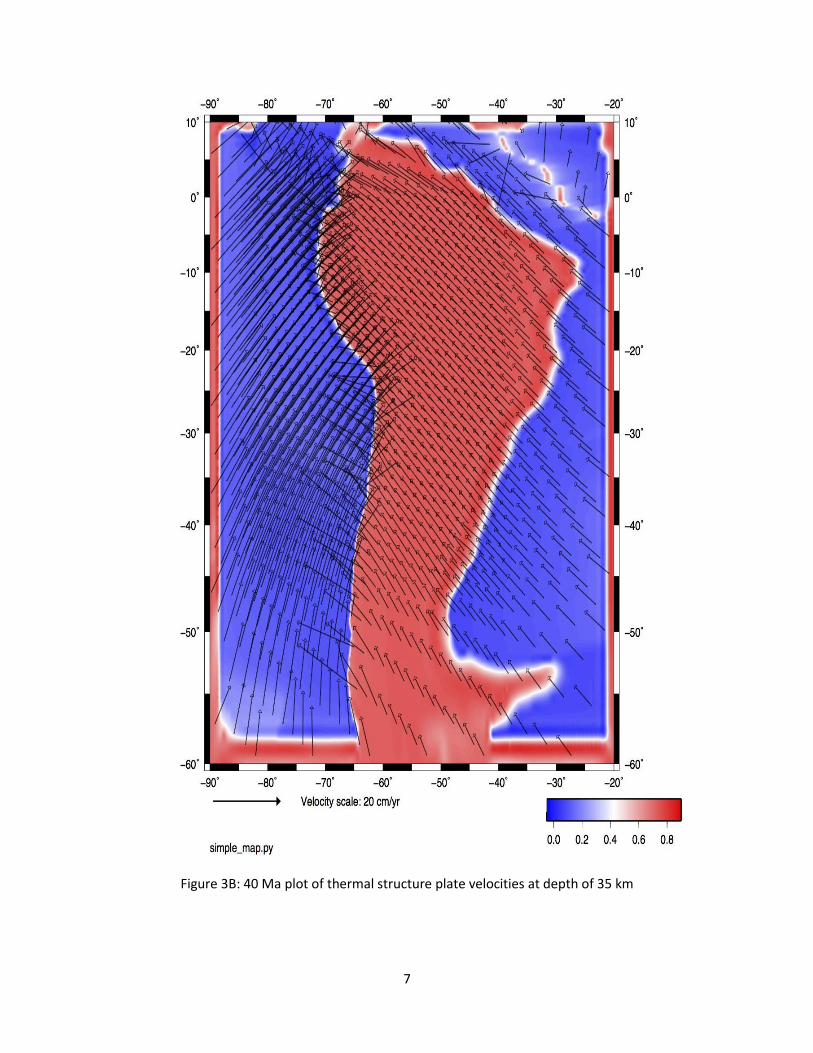
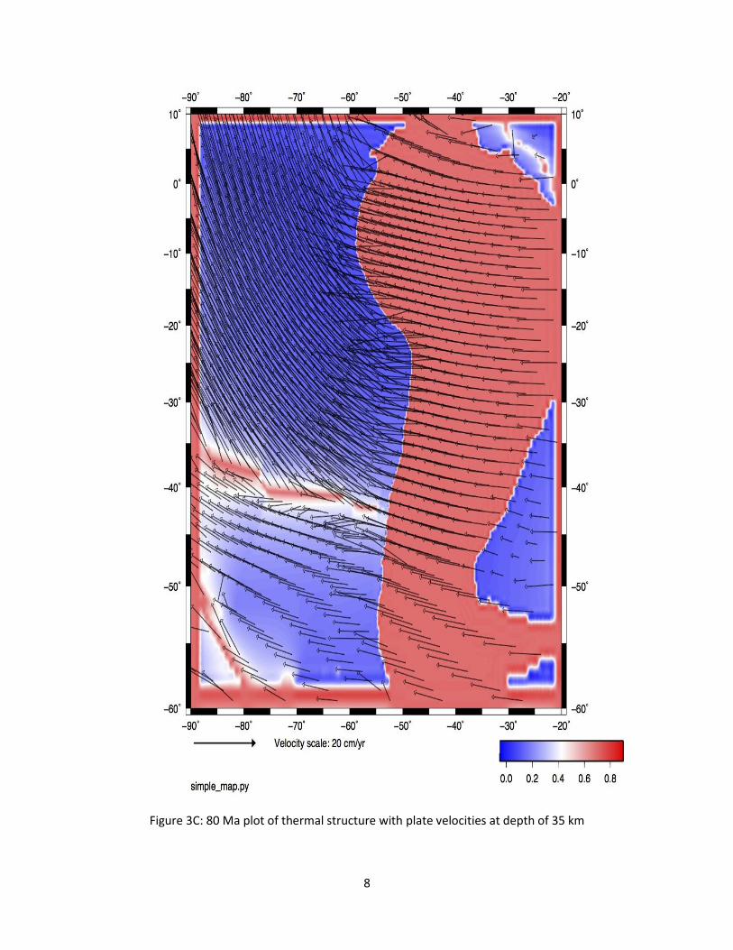
slab geometry. Figure 3 shows these velocity fields at three different geological
times for the reconstruction from Muller et al. (2008).
4) The age of the down-going oceanic lithosphere is another proposed mechanism for
causing flat subduction. Younger oceanic lithosphere is warmer, less dense, and
thus more gravitationally stable than cold slabs. Subduction to the west of South
America has a variation of seafloor ages, ranging from 0 Ma at mid-ocean ridges to
~60 Ma in the central part of the Nazca trench. We will look for correlations
between these ages and their corresponding slab dip angles. In our model, the age
files are produced the same manner as the velocity files, both of which act as
boundary conditions to our subduction models (Figure 5).
6
Figure 3A: Present-day lithosphere thermal structure with plate velocities over-plotted at depth of 35
km. The South American continent is assumed to neutrally buoyant, i.e., at the same temperature as
that of the ambient mantle
7
Figure 3B: 40 Ma plot of thermal structure plate velocities at depth of 35 km
8
Figure 3C: 80 Ma plot of thermal structure with plate velocities at depth of 35 km
9
2.2 Model set-up
To simulate the subduction process, we solve four non-dimensional governing equations
for an incompressible fluid with variable viscosity and Boussinesq approximation. The basic
framework is to solve thermal (eventually thermo-chemical) convection described by the
conservation of mass, momentum and energy.
(1)
(2)
(3)
(4)
where is velocity, dynamic pressure, dynamic viscosity, ambient mantle density,
thermal expansion coefficient, unit vector in the radial direction, T temperature, thermal
diffusivity, C composition, Ra and Rab thermal and compositional Rayleigh numbers, respectively.
The main software for running these 3D subduction models is CitcomS (Zhong et al.,
2000). It is a finite element code that was written to solve thermal convection problems that pertain
to the Earth’s mantle. The XSEDE supercomputer Stampede located at University of Texas-Austin
is used to run the models. Another important software is GPlates (Gurnis et al., 2012), an
interactive paleo-geographic software tool for generating surface files from plate reconstructions
(www.gplates.org). It requires GIS and raster data visualization files to do so. It can generate
boundary conditions such as plate velocities, polygon geometries, etc. These boundary conditions
are then read into CitcomS for the production of models. Plotting figures requires its own software.
Matlab is used to plot simple figures such as trench curvature or craton position at a specific time.
GMT (Generic Mapping Tools) is used to plot out cross-sections at certain latitudes/longitudes
and depth slices (map view) from a finished model run. It can plot temperature, viscosity and
velocities, and this is useful to see features that may appear in one field, but not the other.
We simulate subduction within a finite element mesh of 70° × 70° × 2800 km in the latitude
× longitude × depth directions. The mesh is discretized into 257 × 257 × 65 numerical grids in the
three respective dimensions. A refinement of grid size is applied such that the highest resolution
occurs in the central 2/3 of the mesh and in the upper mantle, with the smallest local grid size of
Ñ×u = 0
-ÑP+Ñ×[h(Ñu+ÑTu)]+ (aRaT +RabC)er = 0
¶T
¶t+u ×ÑT =kÑ2T
¶C
¶t+u ×ÑC = 0
u P h rm a
er k
10
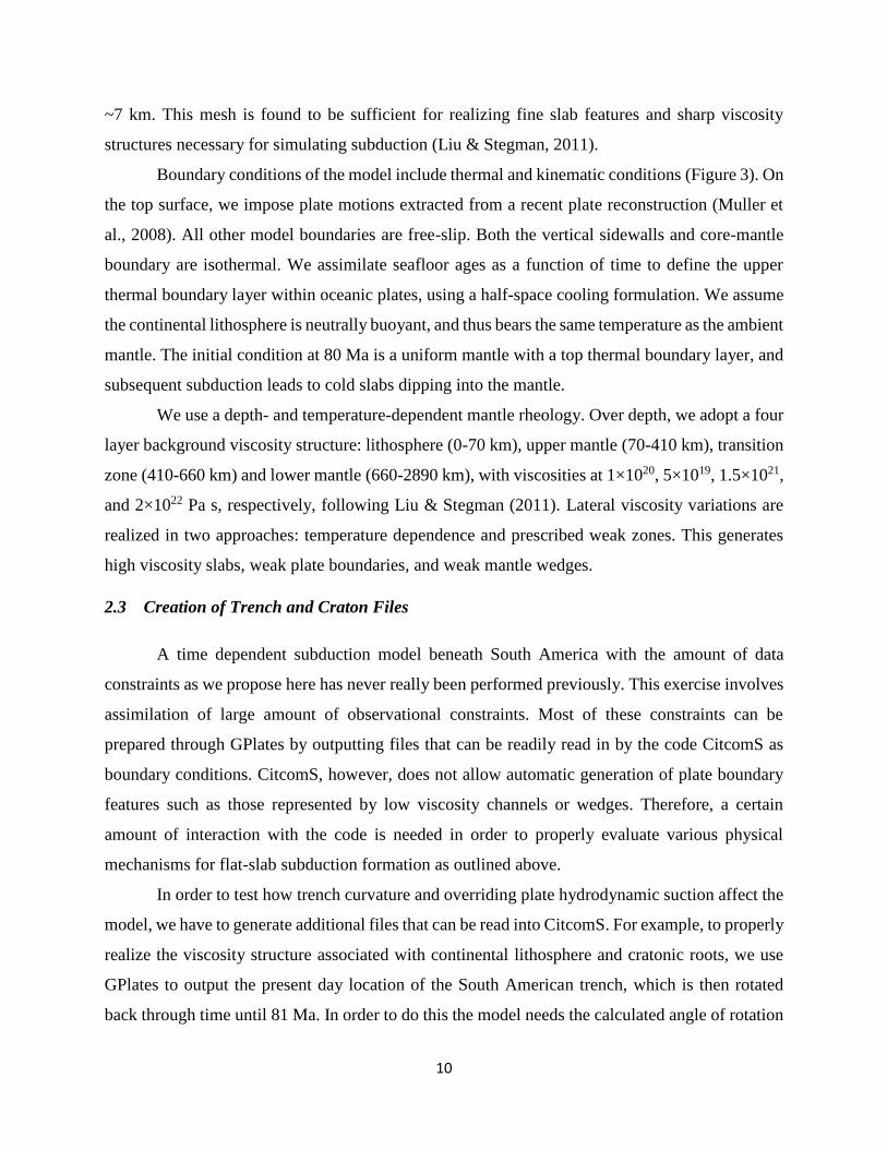
~7 km. This mesh is found to be sufficient for realizing fine slab features and sharp viscosity
structures necessary for simulating subduction (Liu & Stegman, 2011).
Boundary conditions of the model include thermal and kinematic conditions (Figure 3). On
the top surface, we impose plate motions extracted from a recent plate reconstruction (Muller et
al., 2008). All other model boundaries are free-slip. Both the vertical sidewalls and core-mantle
boundary are isothermal. We assimilate seafloor ages as a function of time to define the upper
thermal boundary layer within oceanic plates, using a half-space cooling formulation. We assume
the continental lithosphere is neutrally buoyant, and thus bears the same temperature as the ambient
mantle. The initial condition at 80 Ma is a uniform mantle with a top thermal boundary layer, and
subsequent subduction leads to cold slabs dipping into the mantle.
We use a depth- and temperature-dependent mantle rheology. Over depth, we adopt a four
layer background viscosity structure: lithosphere (0-70 km), upper mantle (70-410 km), transition
zone (410-660 km) and lower mantle (660-2890 km), with viscosities at 1×10²⁰, 5×10¹⁹, 1.5×10²¹,
and 2×10²² Pa s, respectively, following Liu & Stegman (2011). Lateral viscosity variations are
realized in two approaches: temperature dependence and prescribed weak zones. This generates
high viscosity slabs, weak plate boundaries, and weak mantle wedges.
2.3 Creation of Trench and Craton Files
A time dependent subduction model beneath South America with the amount of data
constraints as we propose here has never really been performed previously. This exercise involves
assimilation of large amount of observational constraints. Most of these constraints can be
prepared through GPlates by outputting files that can be readily read in by the code CitcomS as
boundary conditions. CitcomS, however, does not allow automatic generation of plate boundary
features such as those represented by low viscosity channels or wedges. Therefore, a certain
amount of interaction with the code is needed in order to properly evaluate various physical
mechanisms for flat-slab subduction formation as outlined above.
In order to test how trench curvature and overriding plate hydrodynamic suction affect the
model, we have to generate additional files that can be read into CitcomS. For example, to properly
realize the viscosity structure associated with continental lithosphere and cratonic roots, we use
GPlates to output the present day location of the South American trench, which is then rotated
back through time until 81 Ma. In order to do this the model needs the calculated angle of rotation
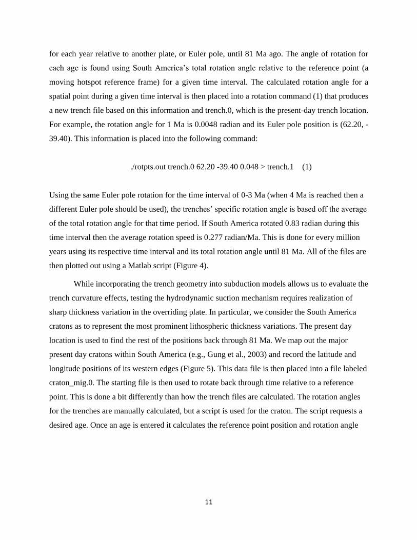
11
for each year relative to another plate, or Euler pole, until 81 Ma ago. The angle of rotation for
each age is found using South America’s total rotation angle relative to the reference point (a
moving hotspot reference frame) for a given time interval. The calculated rotation angle for a
spatial point during a given time interval is then placed into a rotation command (1) that produces
a new trench file based on this information and trench.0, which is the present-day trench location.
For example, the rotation angle for 1 Ma is 0.0048 radian and its Euler pole position is (62.20, -
39.40). This information is placed into the following command:
./rotpts.out trench.0 62.20 -39.40 0.048 > trench.1 (1)
Using the same Euler pole rotation for the time interval of 0-3 Ma (when 4 Ma is reached then a
different Euler pole should be used), the trenches’ specific rotation angle is based off the average
of the total rotation angle for that time period. If South America rotated 0.83 radian during this
time interval then the average rotation speed is 0.277 radian/Ma. This is done for every million
years using its respective time interval and its total rotation angle until 81 Ma. All of the files are
then plotted out using a Matlab script (Figure 4).
While incorporating the trench geometry into subduction models allows us to evaluate the
trench curvature effects, testing the hydrodynamic suction mechanism requires realization of
sharp thickness variation in the overriding plate. In particular, we consider the South America
cratons as to represent the most prominent lithospheric thickness variations. The present day
location is used to find the rest of the positions back through 81 Ma. We map out the major
present day cratons within South America (e.g., Gung et al., 2003) and record the latitude and
longitude positions of its western edges (Figure 5). This data file is then placed into a file labeled
craton_mig.0. The starting file is then used to rotate back through time relative to a reference
point. This is done a bit differently than how the trench files are calculated. The rotation angles
for the trenches are manually calculated, but a script is used for the craton. The script requests a
desired age. Once an age is entered it calculates the reference point position and rotation angle
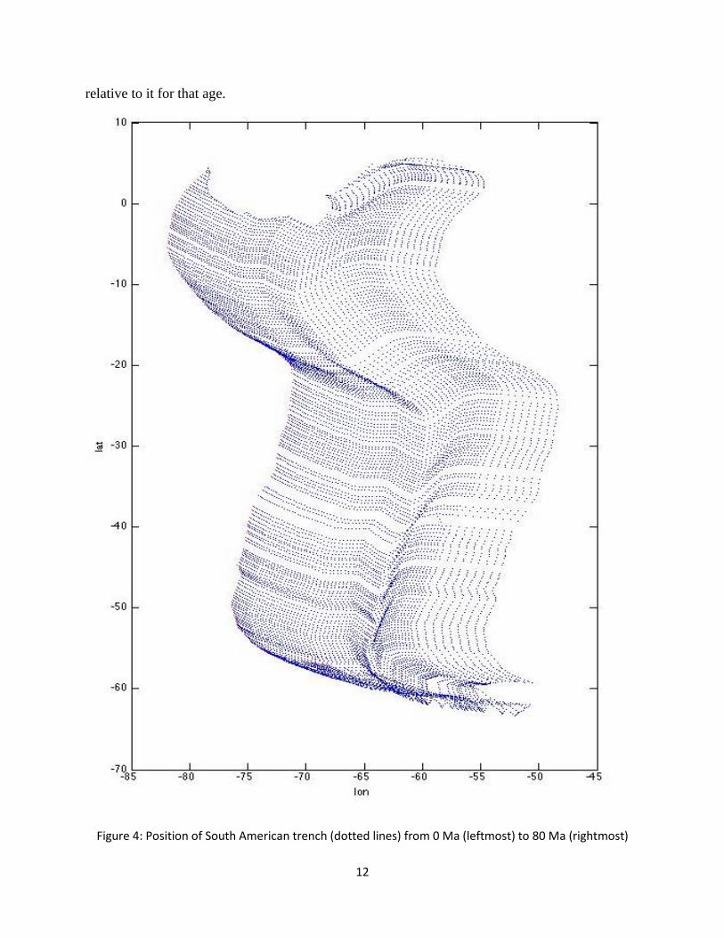
12
relative to it for that age.
Figure 4: Position of South American trench (dotted lines) from 0 Ma (leftmost) to 80 Ma (rightmost)
13
Figure 5: West margin of South American cratons from 0 Ma (leftmost) to 80 Ma (rightmost)
14
CHAPTER 3
PRELIMINARY RESULTS
In order to test the various hypotheses for abnormal subduction as listed in Chapter 2, we
start with the simplest possible subduction model, which by default includes plate kinematics and
lithosphere thermal structure from the recent plate reconstruction of Muller et al. (2008). Beyond
these standard model inputs, we first consider the effect of trench curvature by generating
subduction along the South American trench. In this case, the overriding plate, South America, is
assigned a very weak viscosity (1019 Pa s). Subduction is guided at the surface by kinematic
velocity boundary conditions, and slabs emerge from the top thermal boundary layer defined from
the paleo-seafloor ages. As subduction continues, a physically reasonable subducting slab forms,
where the slab has a larger viscosity than the surrounding mantle due to temperature dependence.
The slab geometry evolves naturally following the position of the subduction zone, in contrast to
conventional parameterized subduction models in which slabs are prescribed rather than self-
emerging.
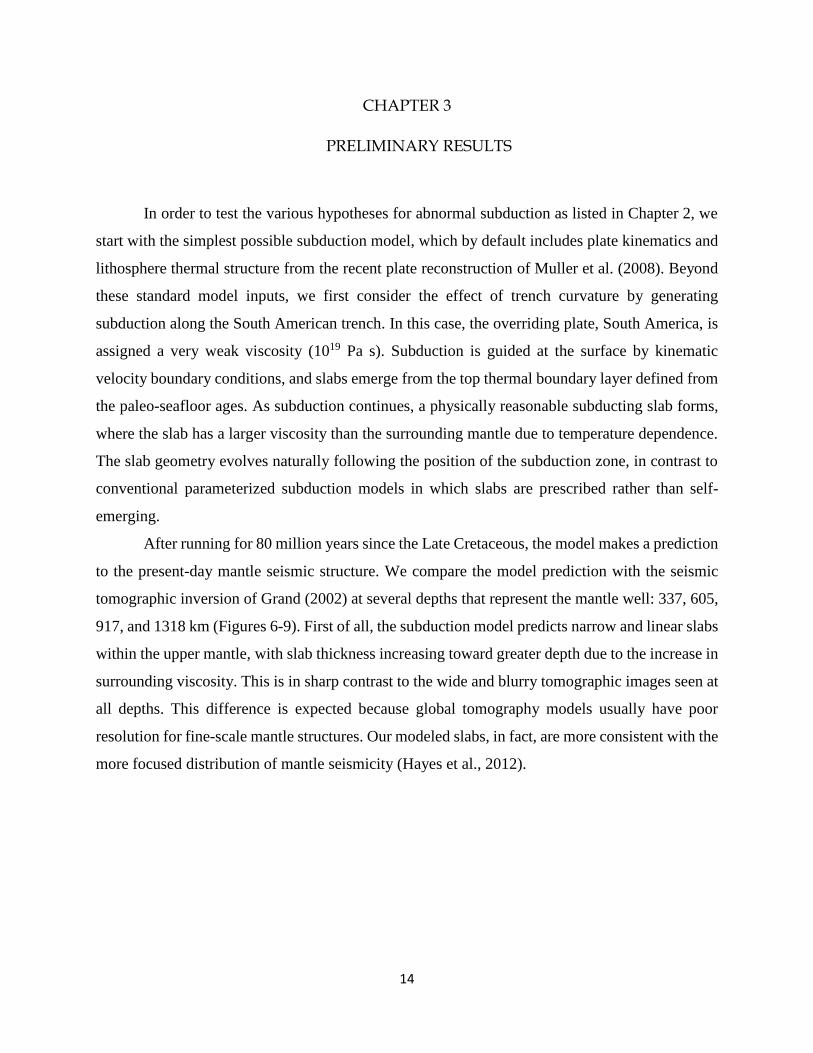
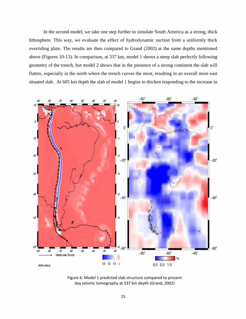
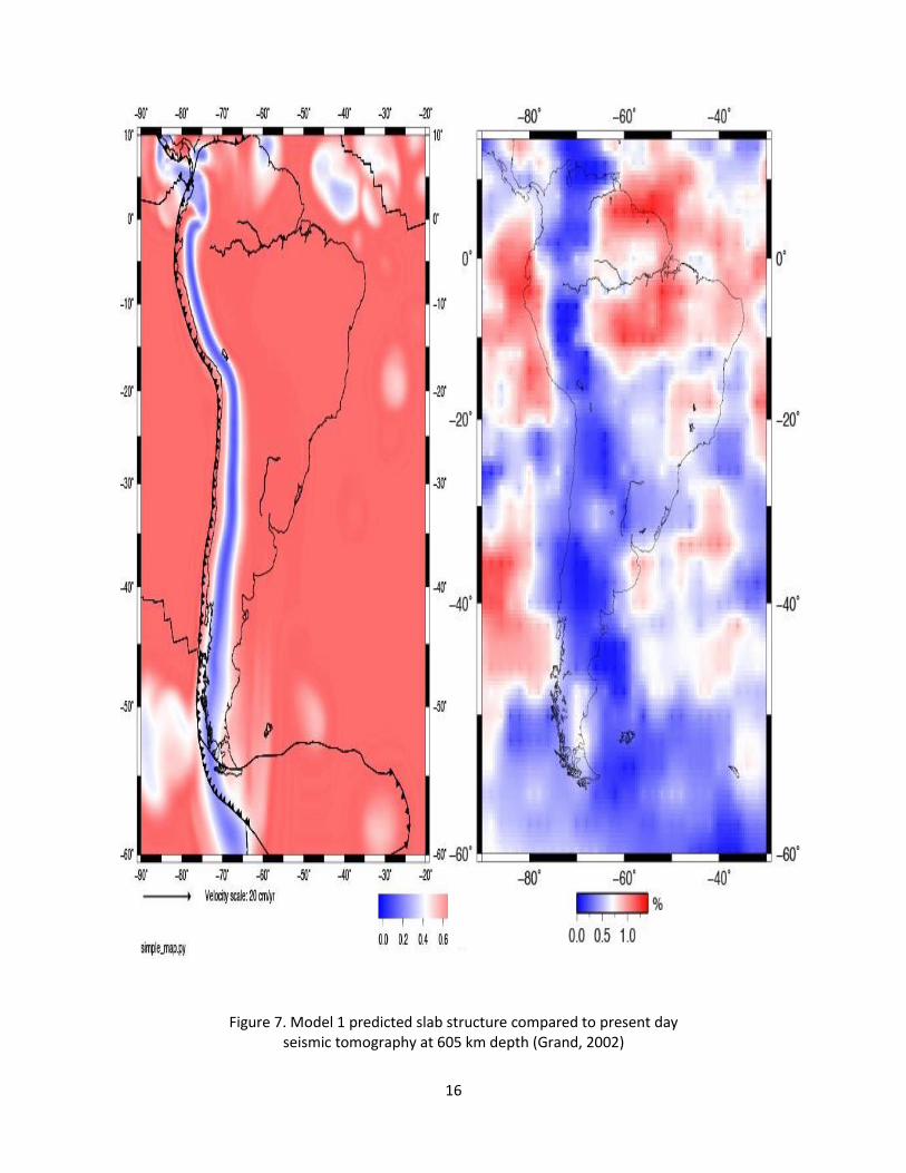
After running for 80 million years since the Late Cretaceous, the model makes a prediction
to the present-day mantle seismic structure. We compare the model prediction with the seismic
tomographic inversion of Grand (2002) at several depths that represent the mantle well: 337, 605,
917, and 1318 km (Figures 6-9). First of all, the subduction model predicts narrow and linear slabs
within the upper mantle, with slab thickness increasing toward greater depth due to the increase in
surrounding viscosity. This is in sharp contrast to the wide and blurry tomographic images seen at
all depths. This difference is expected because global tomography models usually have poor
resolution for fine-scale mantle structures. Our modeled slabs, in fact, are more consistent with the
more focused distribution of mantle seismicity (Hayes et al., 2012).
15
In the second model, we take one step further to simulate South America as a strong, thick
lithosphere. This way, we evaluate the effect of hydrodynamic suction from a uniformly thick
overriding plate. The results are then compared to Grand (2002) at the same depths mentioned
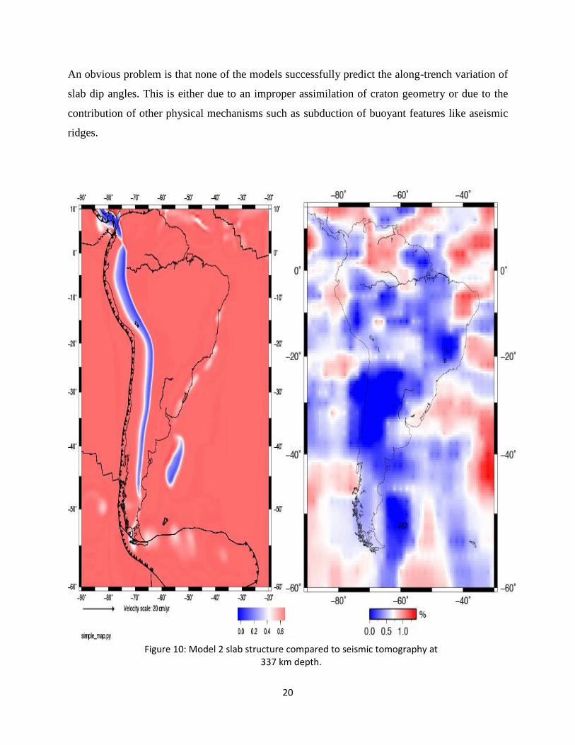
above (Figures 10-13). In comparison, at 337 km, model 1 shows a steep slab perfectly following
geometry of the trench, but model 2 shows that in the presence of a strong continent the slab will
flatten, especially in the north where the trench curves the most, resulting in an overall more east
situated slab. At 605 km depth the slab of model 1 begins to thicken responding to the increase in
Figure 6. Model 1 predicted slab structure compared to present day seismic tomography at 337 km depth (Grand, 2002)
16
Figure 7. Model 1 predicted slab structure compared to present day seismic tomography at 605 km depth (Grand, 2002)
17
Figure 8. Model 1 predicted slab structure compared to present day seismic tomography at 917 km depth (Grand, 2002)
18
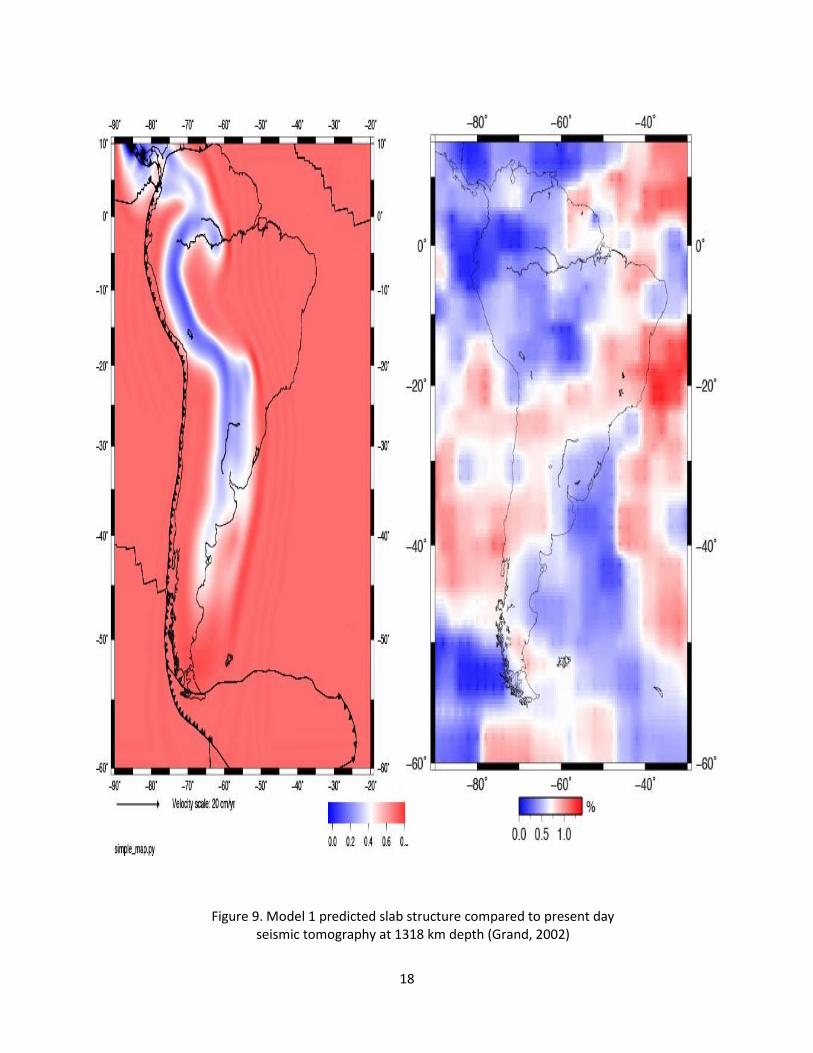
Figure 9. Model 1 predicted slab structure compared to present day seismic tomography at 1318 km depth (Grand, 2002)
19
mantle viscosity, but overall follows the curvature of the trench. Model 2 has more flattening to
the north, and the southern portion of the slab is farther east due to the northwestward motion of
South America during the Cenozoic (e.g., Figure 3B). Both models match the tomography image
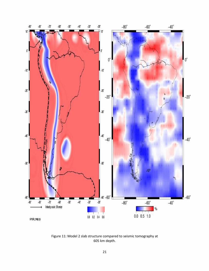
fairly well at this depth, and model 2 does a better job in further matching the part associated with
shallow subduction (Figure 11). The weak continent model (model 1) at 917 km depth follows the
same trend as in its shallower depths, but has a much thicker slab due to the increased mantle
viscosity. The second model produces a slab that is further east at 10 °S, most likely because of
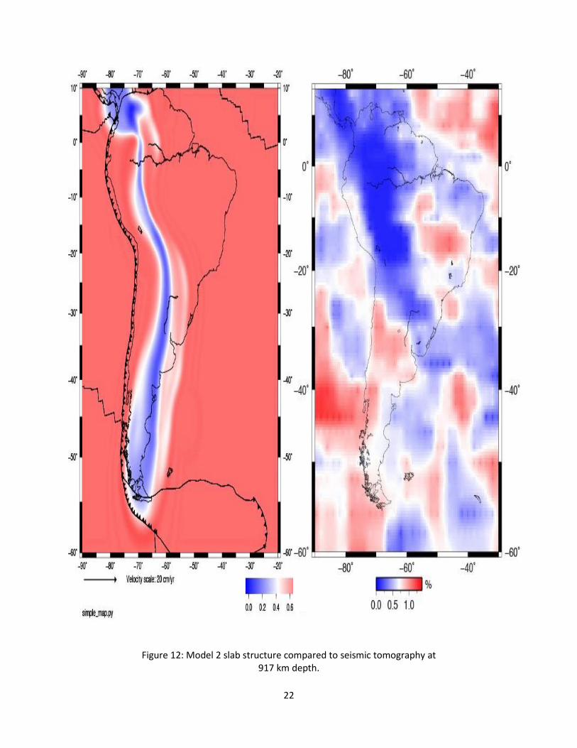
Nazca Plate moving to the NE. The two models produce different slab structure, but only model 2
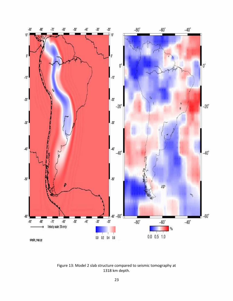
matches present-day tomography somewhat at 917 km depth (Figure 12). At 1318 km depth the
two models have similar slab geometry (model 1 follows the trench a bit more in the northern half)
and almost match tomography except for the apparent gap within the cold anomaly at ~20 °C
(Figure 9 & 13). One interesting detail is that both models show a concentrated cold anomaly at
this depth, where this cold anomaly is mostly in the northern half of South America. This can be
attributed to the existence of a mid-ocean ridge around 80 Ma that causes more cold material to
accumulate on the northern side (Figure 3C)
The mismatch between model and tomography images requires a further tuning of model
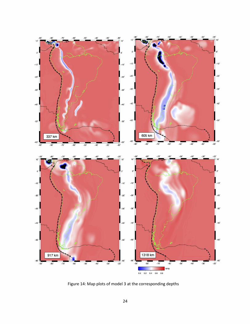
parameters, among which assimilating over-thickened cratons represents an option. Model 2 tested
the hydrodynamic suction from a uniform lithosphere, and the next model will incorporate all of
the same details as in model 2 except that it now has more localized sections of hydrodynamic
suction due to the restricted areas of cratons. Model 3 further improves the match with tomography
(Figure 14) at lower mantle depths. However, the upper mantle fits still need improvement, in that
modeled slabs are more easterly than the tomography images show. This suggests that testing other
mechanisms for flat-slab formation is necessary, which will be subject to future research.
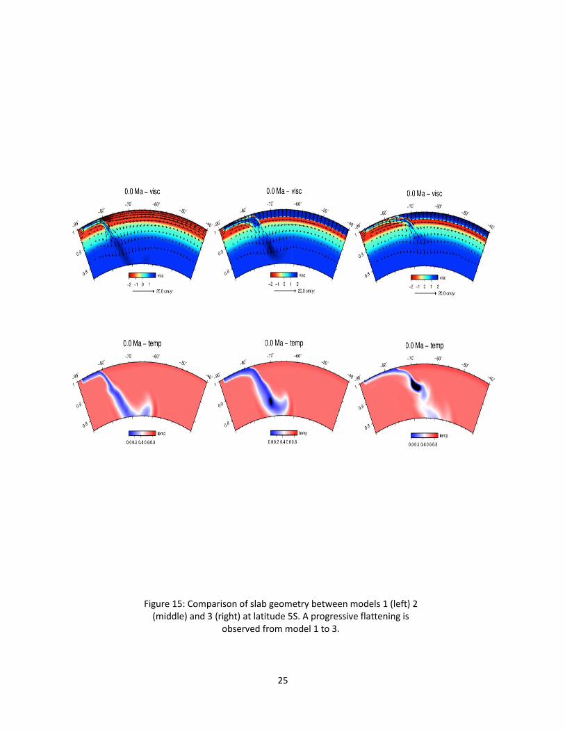
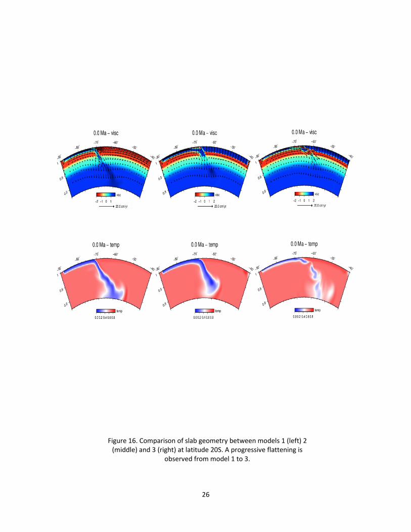
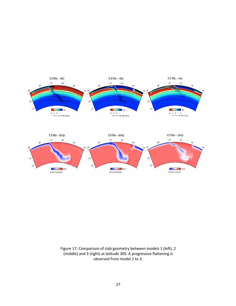
Collectively, we compare the three models by showing cross-sections at latitudes of 5̊ S,
20̊ S, and 30̊ S, respectively (Figures 15-17). Along all three cross sections in model 1, there is no
flat-slab formation, indicating that the trench curvature itself is not enough to flatten the slab, even
though the slab is much stronger than the ambient model. Model 2 predicts a systematic shallowing
of slabs at all three cross sections. This is consistent with an overall increase hydrodynamic suction
from the overriding plate. Model 3 further increases the hydrodynamic suction force where a craton
is adjacent to the trench, and causes the slab to go sub-horizontally beneath the overriding cratons.
20
An obvious problem is that none of the models successfully predict the along-trench variation of
slab dip angles. This is either due to an improper assimilation of craton geometry or due to the
contribution of other physical mechanisms such as subduction of buoyant features like aseismic
ridges.
Figure 10: Model 2 slab structure compared to seismic tomography at 337 km depth.
21
Figure 11: Model 2 slab structure compared to seismic tomography at 605 km depth.
22
Figure 12: Model 2 slab structure compared to seismic tomography at 917 km depth.
23
Figure 13: Model 2 slab structure compared to seismic tomography at 1318 km depth.
24
Figure 14: Map plots of model 3 at the corresponding depths
25
Figure 15: Comparison of slab geometry between models 1 (left) 2 (middle) and 3 (right) at latitude 5S. A progressive flattening is
observed from model 1 to 3.
26
Figure 16. Comparison of slab geometry between models 1 (left) 2 (middle) and 3 (right) at latitude 20S. A progressive flattening is
observed from model 1 to 3.
27
Figure 17: Comparison of slab geometry between models 1 (left), 2 (middle) and 3 (right) at latitude 30S. A progressive flattening is
observed from model 1 to 3.
28
CHAPTER 4
CONCLUSION AND FUTURE WORK
We simulate the subduction history beneath South America since Late Cretaceous. By
gradually adding in model complexities including trench curvature, a strong overriding plate, and
isolated thick cratons, the models demonstrate a progressive change in slab behavior and provide
results that better match tomographic images, leading towards the objective of this study. We were
able to recreate flat subduction at latitudes where we see flat slabs today in Model 3 with thick
craton roots, but not the variation from flat to steep. Places to improve include model match with
tomography at depths, especially inside the upper mantle. On the one hand, it is necessary to collect
better mantle seismic images including more tomography models, especially high-resolution
regional models, and slab geometry constrained by seismicity distribution (e.g., Hayes et al.,
2012). On the other hand, we still need to produce more realistic subduction models, including
better describing the geometry of cratons and assimilating buoyancy structures in the subduction
plate. Another aspect of improvement is to better simulate the subduction process within Middle
America. Our current model does not realize the viscosity structure and trench geometry of the
Middle American subduction system, due to its complex subduction history. Inclusion of this part
will likely increase the prediction of seismic structure on the northernmost part of South America
(Figures 6-14). Another major next step is to incorporate over-thickened oceanic crust into our
model. This type of work on South America has not been previously performed. Any progress on
this study is important to the understanding of flat-slab subduction dynamics, as well as a better
constraint on the mantle structure itself, given the still low seismic resolution in existing
tomographic inversions in this part of the world.
29
References
Gerya, T.V., Fossati, D., Cantieni, C., and Seward, D., 2009, Dynamic effects of aseismic ridge
subduction: Numerical modelling: European Journal of Mineralogy, 21, 649–661, doi:10.1127/
0935-1221/2009/0021-1931.
Grand, S. P., 2002, Mantle shear–wave tomography and the fate of subducted slabs, Phi. Trans.
Roy. Soc. Lond., Ser. A., 360, 2475-2491.
Gung, Y., M. Panning, and B. Romanowicz, 2003, Global anisotropy and the thickness of
continents, Nature, 422, 707–711, doi:10.1038/nature01559.
Gurnis, M., M. Turner, S. Zahirovic, L. DiCaprio, S. Spasojevic, R. D. Müller, J. Boyden, M.
Seton, V. C. Manea, and D. J. Bower, 2012, Plate tectonic reconstructions with continuously
closing plates, Computers & Geosciences, 38, 35-42.
Gutscher, M.-A., J.-L. Olivet, D. Aslanian, R. Maury, and J.-P. Elssen, The 'lost Inca Plateau':
Cause of fiat subduction beneath Peru? Earth Planet. Sci. Lett., 171, 335-341, 1999.
Gutscher M-A., Spakman, W., Bijwaard, H. & Engdahl, E.R., Geodynamics of flat subduction:
seismicity and tomographic constraints from the Andean margin, Tectonics, 19, 814-833 (2000).
Hayes, G. P., Wald, D. J., and Johnson, R. L., 2012, Slab1.0: A three‐ dimensional model of
global subduction zone geometries, J. Geophys. Res., 117, B01302, doi:10.1029/2011JB008524.
Liu, L., Gurnis, M., Seton, M., Saleeby, J., Müller, R.D., & Jackson, J. M., 2010, The role of
oceanic plateau subduction in the Laramide orogeny, Nature Geoscience 3 (5), 353-357.
Liu, L. & Stegman, D.R., Segmentation of the Farallon slab, Earth Planet. Sci. Lett., 311(1), 1-10
(2011).
30
Manea, V. C., Pérez-Gussinyé, M. and Manea, M., 2012, Chilean flat slab subduction controlled
by overriding plate thickness and trench rollback, 40, 35-38, doi:10.1130/G32543.1.
Müller, R. D., Sdrolias, M., Gaina, C., Roest, W., 2008, Age, spreading rates, and spreading
asymmetry of the world's ocean crust, Geochemistry, Geophysics, Geosystems, 9 (4).
Coney, P. J. and Reynolds, S. J., 1977, Cordilleran Benoiff zones, Nature, 270, 403-406.
Ritsema J, van Heijst HJ, Woodhouse JH, Complex shear wave velocity structure imaged
beneath Africa and Iceland, Science, 286, 1925–1928, 1999.
Stevenson, D.J., and Turner, S.J., 1977, Angle of subduction: Nature, 270, 334–336,
doi:10.1038/270334a0.
van Hunen, J., van der Berg, A.P., and Vlaar, N.J., 2004, Various mechanisms to induce present-
day flat subduction and implications for the younger Earth: A numerical parameter study:
Physics of the Earth and Planetary Interiors, 146, 179–194, doi:10.1016/j.pepi.2003.07.027.
Zhong, S., Zuber, M. T., Moresi, L., and Gurnis, M., 2000, The role of temperature-dependent
viscosity and surface plates in spherical shell models of mantle convection, Journal of
Geophysical Research, 105, 11,063-11,082.