investigating low energy wireless networks for the

Investigating Low Energy Wireless Networks for theInternet of Things

Branden Ghena

Electrical Engineering and Computer SciencesUniversity of California at Berkeley

Technical Report No. UCB/EECS-2020-209http://www2.eecs.berkeley.edu/Pubs/TechRpts/2020/EECS-2020-209.html

December 17, 2020

Copyright © 2020, by the author(s).All rights reserved.

Permission to make digital or hard copies of all or part of this work forpersonal or classroom use is granted without fee provided that copies arenot made or distributed for profit or commercial advantage and that copiesbear this notice and the full citation on the first page. To copy otherwise, torepublish, to post on servers or to redistribute to lists, requires prior specificpermission.

Investigating Low Energy Wireless Networks for the Internet of Things

by

Branden R. Ghena

A dissertation submitted in partial satisfaction of the

requirements for the degree of

Doctor of Philosophy

in

Electrical Engineering and Computer Science

in the

Graduate Division

of the

University of California, Berkeley

Committee in charge:

Associate Professor Prabal Dutta, ChairProfessor David CullerProfessor Scott Shenker

Associate Professor Philip Levis

Fall 2020


Copyright 2020by

Branden R. Ghena

1

Abstract


by

Branden R. Ghena

Doctor of Philosophy in Electrical Engineering and Computer Science

University of California, Berkeley

Associate Professor Prabal Dutta, Chair

The Internet of Things (IoT) encompasses a broad array of technologies that connect thephysical world with large-scale data processing and storage. Today, we can build ultra-lowpower devices that last for decades on ambient energy and we can deploy highly scalableinternet services to process streams of IoT data. The dominant challenge of IoT lies in con-necting these two domains. To meet this challenge, many new networks have been developedwith low-energy, low-throughput, and predominantly uplink use cases in mind.

In this work, we explore the capabilities and limitations of several recent IoT-focused net-works. While these novel networks are not yet deployed at scale, modeling aspects of themenables us to predict the success or failure of particular applications and explore the ramifi-cations of potential protocol improvements.

In the local-area domain, Bluetooth Low Energy (BLE) has arisen as an ubiquitous method ofconnecting deployed devices directly to users’ smartphones. One communication mechanismthat BLE provides is the advertisement—a simple, periodic, broadcast message intended fordevice discovery. With advertisements, we can create a single-hop, star-topology network infull compliance with the BLE specification that allows any number of devices to send datato any number of gateways. By modeling advertisement transmissions, we can accuratelypredict congestion in advertisement networks, which enables an a priori understanding ofperformance and an in-situ adaptation mechanism to meet reliability expectations.

In the wide-area domain, multiple low-power, wide-area networks (LPWANs) have arisento enable city-scale deployments. Their ability to transmit at ranges over a kilometer whiledrawing only a few hundred milliwatts could enable exciting new applications. To understandLPWAN capabilities, we propose a new metric, bit flux, which describes communication interms of throughput over a coverage area. By using bit flux to model the performance ofnetworks and the needs of applications, we demonstrate problems with the existing designsof several LPWANs that make them unsuitable for many real-world deployments.

2

In both domains, we explore the strengths and weaknesses of communication technologies andtheir potential to serve real-world applications. The potential for these networks to promotea new generation of easy-to-deploy sensors is high. However, through the application ofcommunication models, we demonstrate both potential use cases and also very real concernsthat may limit them. By uncovering concerns that future deployments will face, we hope toguide improvements to these protocols that will improve their use and support the growthof the Internet of Things.

i

To my family and my friends.I have been blessed by your love.

ii

Acknowledgments

I was surprised to discover in high school that engineering was a field that I would beinterested in. I was surprised in college when I ended up deciding that after five yearsof undergraduate studies, going on to more school would be the best path for me. I wassurprised when teaching, not research, ended up being the part of grad school I loved themost. I was surprised every step of the way. No one else was. My family and friends hadalready seen and long encouraged in me things that took me years to realize for myself. Iam so very lucky to have them in my life.

My parents, Robert and Denise Ghena, have always supported me in my endeavors.They were excited no matter if it was a spelling bee, a FIRST robotics competition, ordeciding to stay in school even longer. They have helped me move, driven hours throughsnowstorms to pick me up, and always been there when I needed to talk. I have been solucky to have them with me, knowing that they will support me however I need. Nate andChelsea Ghena, my brother and sister-in-law, have been my allies as well. They are alwaysthere to share sarcastic jokes with, and have understood my struggles. We have more degreesbetween us than is reasonable. My extended family have been insanely loving, and spendingholidays with them is my favorite thing. That my grandparents could be online for mydissertation talk was a wonderful gift.

In school I was supported by Ben Naveaux and Andy Felder, who kept me social andshared many laughs with me over D&D. Getting to grow up with them has been an honor,as has been watching our group grow with Jessica Felder and the kids. In college, I waslucky enough to stumble into the most amazing hall. The perfect mix of scholarship andstrangeness that was exactly what I needed. I miss the Laurium House, icicles and all,and the weekends spent in the living room laughing and complaining as Cameron Kardel orSam Dietrick played games. We got work done occasionally as well, and many a long nightwas spent on campus working with Andy Mauragis, Andrew Maine, and Kevin Nelson. AsI navigated the academic job market and graduating, Charlotte Rosenfield was there tosupport and love me through my anxieties and my celebrations.

At Michigan Tech, I have Dr. Brad King and Dr. Roger Kieckhafer to thank for leadingme down the path to graduate school. Working on Oculus-ASR made me the engineer I amtoday. Even back then I worked on the radios, computer hardware, and software systems.At Michigan, Dr. Mark Brehob demonstrated the combination of compassion and capabilitythat I hope to approach in my own teaching. In my research life, Dr. Phil Levis taught methoughtful design practices and that even as a professor, you are still an engineer as well.

Dr. Prabal Dutta gave me the opportunity to take my knowledge and build upon it aspart of Lab11. He reminded me to always focus on why the research we do is important andwhat its impacts are. He taught me that being able to explain research through writing andspeech is the most valuable skill that grad school provides. He also made it clear that thereare many paths towards being successful in academia, and when I realized that teaching wasmy path, he supported me through it without fail.

iii

Finally, I want to thank Lab11 and friends. I felt like the dumbest person in the roomfor years, but that meant I was able to learn from all of you. Ye-Sheng Kuo spent yearsteaching me how to fix my soldering mistakes. Sam Debruin brought me in to help onPowerBlade, which led me down the path of this dissertation, and helped me to become abetter writer. Brad Campbell and Pat Pannuto were my collaborators on Tock, along withAmit Levy, and taught me to fight for the projects I believed in. They were my inspirationson how to be a grad student. Meghan Clark, Noah Klugman, and Will Huang provided muchneeded emotional support. We were always allies as the second wave of lab members. JoshAdkins and Neal Jackson were undergraduates when I met them and my colleagues when Ileft. We spent many productive afternoons together discussing research possibilities. Themany master’s students, undergrads, and high schoolers who I got to work with along theway inspired me to stay on the teaching path. The rest of Lab11 and friends: Ben Kempke,Thomas Zachariah, Rohit Ramesh, David Adrian, Matt Podolsky, Jean-Luc Watson, ShishirPatil, Andreas Biri, and others were there as parts of my daily life and helped with countlesspractice talks and paper revisions. My time in grad school was made perfect for having spentit with all of you.

iv

Contents

Acknowledgements ii

Contents iv

List of Figures vii

List of Tables xiii

1 Introduction 11.1 Bluetooth Low-Energy Local Communication . . . . . . . . . . . . . . . . . 21.2 Low-Power Wide-Area Networks . . . . . . . . . . . . . . . . . . . . . . . . . 41.3 Thesis Statement . . . . . . . . . . . . . . . . . . . . . . . . . . . . . . . . . 51.4 Contributions of this Dissertation . . . . . . . . . . . . . . . . . . . . . . . . 5

2 BLE Background 72.1 Bluetooth Low Energy Overview . . . . . . . . . . . . . . . . . . . . . . . . 7

2.1.1 Advertising . . . . . . . . . . . . . . . . . . . . . . . . . . . . . . . . 72.1.2 Scanning . . . . . . . . . . . . . . . . . . . . . . . . . . . . . . . . . . 92.1.3 Scan Requests . . . . . . . . . . . . . . . . . . . . . . . . . . . . . . . 92.1.4 Connections . . . . . . . . . . . . . . . . . . . . . . . . . . . . . . . . 102.1.5 BLE 5.0 . . . . . . . . . . . . . . . . . . . . . . . . . . . . . . . . . . 10

2.2 Advertisement Use Cases . . . . . . . . . . . . . . . . . . . . . . . . . . . . . 112.2.1 Beacons . . . . . . . . . . . . . . . . . . . . . . . . . . . . . . . . . . 112.2.2 Tracking . . . . . . . . . . . . . . . . . . . . . . . . . . . . . . . . . . 122.2.3 Proximal Communication . . . . . . . . . . . . . . . . . . . . . . . . 132.2.4 Periodic Sensing . . . . . . . . . . . . . . . . . . . . . . . . . . . . . . 14

2.3 Summary . . . . . . . . . . . . . . . . . . . . . . . . . . . . . . . . . . . . . 15

3 Modeling BLE Advertisements 163.1 Collisions . . . . . . . . . . . . . . . . . . . . . . . . . . . . . . . . . . . . . 16

3.1.1 Modeling Packet Reception . . . . . . . . . . . . . . . . . . . . . . . 173.1.2 Modeling Data Reception . . . . . . . . . . . . . . . . . . . . . . . . 203.1.3 Advertisement Network Takeaways . . . . . . . . . . . . . . . . . . . 23

v

3.1.4 Empirical Testing . . . . . . . . . . . . . . . . . . . . . . . . . . . . . 243.2 Energy . . . . . . . . . . . . . . . . . . . . . . . . . . . . . . . . . . . . . . . 263.3 Applying Models . . . . . . . . . . . . . . . . . . . . . . . . . . . . . . . . . 28

3.3.1 BLE Protocol . . . . . . . . . . . . . . . . . . . . . . . . . . . . . . . 283.3.2 Contact Tracing . . . . . . . . . . . . . . . . . . . . . . . . . . . . . . 31

3.4 Summary . . . . . . . . . . . . . . . . . . . . . . . . . . . . . . . . . . . . . 32

4 BLE Deployment Studies 334.1 Powerblade Deployment . . . . . . . . . . . . . . . . . . . . . . . . . . . . . 33

4.1.1 Expected Reception Rates . . . . . . . . . . . . . . . . . . . . . . . . 354.1.2 Measured Data Reception Rates . . . . . . . . . . . . . . . . . . . . . 364.1.3 Packet Reception . . . . . . . . . . . . . . . . . . . . . . . . . . . . . 374.1.4 Gateway Analysis . . . . . . . . . . . . . . . . . . . . . . . . . . . . . 39

4.2 Statically Planned Deployments . . . . . . . . . . . . . . . . . . . . . . . . . 414.2.1 Revising Deployment Parameters . . . . . . . . . . . . . . . . . . . . 414.2.2 Deployment Results . . . . . . . . . . . . . . . . . . . . . . . . . . . . 42

4.3 Adapting to the BLE Environment . . . . . . . . . . . . . . . . . . . . . . . 454.3.1 Measurement Method . . . . . . . . . . . . . . . . . . . . . . . . . . 454.3.2 Measurement Frequency . . . . . . . . . . . . . . . . . . . . . . . . . 454.3.3 Measurement Duration . . . . . . . . . . . . . . . . . . . . . . . . . . 464.3.4 Measurement Energy Cost . . . . . . . . . . . . . . . . . . . . . . . . 464.3.5 Adaptation . . . . . . . . . . . . . . . . . . . . . . . . . . . . . . . . 474.3.6 Experimental Results . . . . . . . . . . . . . . . . . . . . . . . . . . . 48

4.4 Summary . . . . . . . . . . . . . . . . . . . . . . . . . . . . . . . . . . . . . 51

5 LPWAN Background 535.1 Unlicensed LPWANs . . . . . . . . . . . . . . . . . . . . . . . . . . . . . . . 54

5.1.1 Sigfox . . . . . . . . . . . . . . . . . . . . . . . . . . . . . . . . . . . 545.1.2 LoRaWAN . . . . . . . . . . . . . . . . . . . . . . . . . . . . . . . . . 555.1.3 Other protocols . . . . . . . . . . . . . . . . . . . . . . . . . . . . . . 55

5.2 Cellular Networks . . . . . . . . . . . . . . . . . . . . . . . . . . . . . . . . . 575.2.1 GPRS . . . . . . . . . . . . . . . . . . . . . . . . . . . . . . . . . . . 575.2.2 LTE-M . . . . . . . . . . . . . . . . . . . . . . . . . . . . . . . . . . . 575.2.3 NB-IoT . . . . . . . . . . . . . . . . . . . . . . . . . . . . . . . . . . 58

5.3 Summary . . . . . . . . . . . . . . . . . . . . . . . . . . . . . . . . . . . . . 58

6 Modeling Wide-Area Communication 596.1 Network Characteristics . . . . . . . . . . . . . . . . . . . . . . . . . . . . . 59

6.1.1 Throughput and Range . . . . . . . . . . . . . . . . . . . . . . . . . . 596.1.2 Power Comparison . . . . . . . . . . . . . . . . . . . . . . . . . . . . 60

6.2 Network Bit Flux . . . . . . . . . . . . . . . . . . . . . . . . . . . . . . . . . 616.3 Pervasive Applications . . . . . . . . . . . . . . . . . . . . . . . . . . . . . . 64

vi

6.4 Summary . . . . . . . . . . . . . . . . . . . . . . . . . . . . . . . . . . . . . 66

7 LPWAN Capabilities 677.1 Network Suitability . . . . . . . . . . . . . . . . . . . . . . . . . . . . . . . . 67

7.1.1 H1N1 Case Study . . . . . . . . . . . . . . . . . . . . . . . . . . . . . 687.1.2 Electricity Metering Case Study . . . . . . . . . . . . . . . . . . . . . 697.1.3 Are LPWANs Sufficient? . . . . . . . . . . . . . . . . . . . . . . . . . 71

7.2 Network Solutions . . . . . . . . . . . . . . . . . . . . . . . . . . . . . . . . . 727.2.1 Improving Transmission . . . . . . . . . . . . . . . . . . . . . . . . . 737.2.2 Resilient Reception . . . . . . . . . . . . . . . . . . . . . . . . . . . . 737.2.3 Increasing Bandwidth . . . . . . . . . . . . . . . . . . . . . . . . . . 747.2.4 Coexisting through Coordination . . . . . . . . . . . . . . . . . . . . 75

7.3 Summary . . . . . . . . . . . . . . . . . . . . . . . . . . . . . . . . . . . . . 76

8 Conclusion 78

Bibliography 80

vii

List of Figures

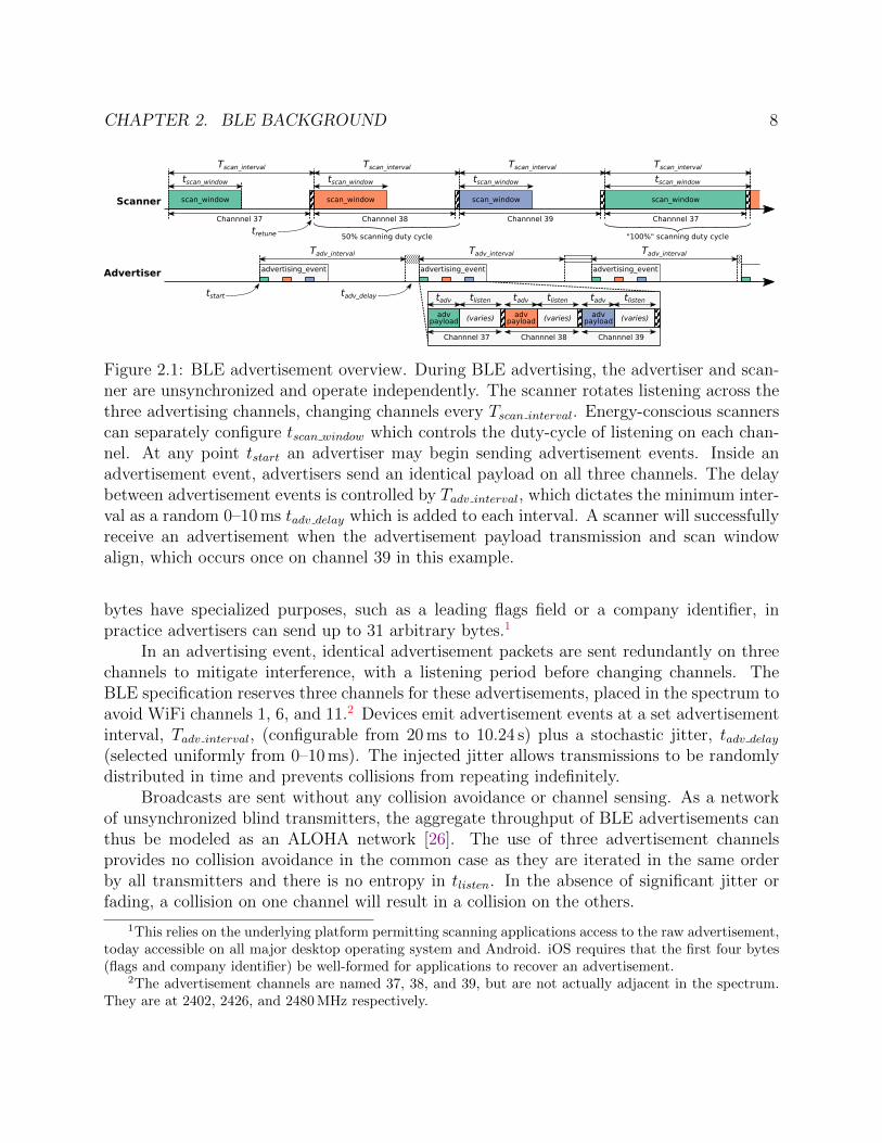
2.1 BLE advertisement overview. During BLE advertising, the advertiser and scan-ner are unsynchronized and operate independently. The scanner rotates listen-ing across the three advertising channels, changing channels every Tscan interval.Energy-conscious scanners can separately configure tscan window which controls theduty-cycle of listening on each channel. At any point tstart an advertiser may beginsending advertisement events. Inside an advertisement event, advertisers send anidentical payload on all three channels. The delay between advertisement eventsis controlled by Tadv interval, which dictates the minimum interval as a random 0–10 ms tadv delay which is added to each interval. A scanner will successfully receivean advertisement when the advertisement payload transmission and scan windowalign, which occurs once on channel 39 in this example. . . . . . . . . . . . . . 8

2.2 Protocol format for common BLE beacon types. The default BLE PDU is shownin gray, with advertising protocol data unit in blue. Both iBeacon and Eddystoneuse BLE advertisements to broadcast information. The iBeacon format uses a 16-byte UUID along with major and minor numbers to identify devices and locations.The Eddystone URL format allows a location for a web resource to be broadcast.Both beacon formats enable the connection of physical objects and places tovirtual identities and resources. . . . . . . . . . . . . . . . . . . . . . . . . . . . 12

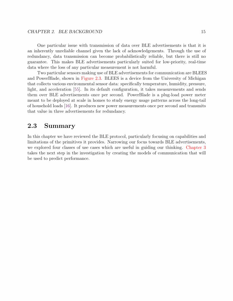
2.3 BLEES and PowerBlade. At left is BLEES: an environmental sensor capableof sensing temperature, humidity, pressure, light, and acceleration. At rightis PowerBlade: a low-profile, plug-load power meter. Both sensors broadcastperiodic measurements using BLE advertisements. . . . . . . . . . . . . . . . . 14

3.1 Packet reception rates as deployment size increases. Both the worst case (31 bytepayload broadcast every 20 ms) and best case (0 byte payload broadcast every10240 ms) are displayed. The configuration for PowerBlade [16], a research BLEsensor node that transmits a 23 byte payload every 200 ms, is also included as areal-world example. For small deployments (fewer than 10 nodes), any configu-rations will likely result in acceptable PRR. As deployments scale, however, theymust balance desired throughput and reception rate. . . . . . . . . . . . . . . . 18

viii

3.2 Minimum advertising intervals to realize target packet error rates. Given a fixedpayload (here 31 bytes), to realize a target packet error rate the minimum adver-tising interval must grow with the number of devices. Even small deploymentsrequire several hundred milliseconds between transmissions to achieve a 1% packeterror rate. Accepting 10% error rates allows sub-second intervals even as deploy-ments expand to one hundred devices. . . . . . . . . . . . . . . . . . . . . . . . 19

3.3 Probability of a repeat packet collision. A repeat collision occurs if the differencein delays applied to each previous colliding transmission is less than the size of thecollision window. The difference in uniform random variables (the delays) createsa triangular distribution, which can be integrated across the collision windowto determine the probability of a repeat collision. The resulting repeat collisionprobability is significantly higher than the original probability of an uncorrelatedcollision. . . . . . . . . . . . . . . . . . . . . . . . . . . . . . . . . . . . . . . . 20

3.4 Collision probability for two devices. The probability of a collision between twoBLE transmitters grows as the payload size of the packet increases. The generalprobability of collision is plotted for several advertising intervals. The probabilityof a repeat collision is increased due to the periodicity of BLE. Given a collisionon the previous packet, the probability of collision for the current transmission inBLE is twice as high as the normal probability for even the fastest advertisementinterval. . . . . . . . . . . . . . . . . . . . . . . . . . . . . . . . . . . . . . . . . 22

3.5 Data reception rate for redundant transmissions. The number of redundant pack-ets transmitted is varied for multiple deployment sizes, each transmitting at a20 ms interval except the 100 device scenario which considers both 20 ms and100 ms intervals. As the density of a deployment grows, advertisers need to senda greater number of redundant packets to maintain data reception reliability. La-tency and throughput also affect reception rate, slowing advertising from 20 to100 ms improves reception at the expense of responsiveness and throughput. Atzero redundant packets, the reception rate is identical to packet reception rate.For higher values, reception of any one packet is enough to receive the data.Sending redundant packets can significantly improve data reception when thereis contention in the network. . . . . . . . . . . . . . . . . . . . . . . . . . . . . 23

3.6 Data reception rate favors redundancy. Data reception rates are compared forone network configured to send a packet every 1000 ms versus another configuredto send five redundant packets per second at 200 ms intervals across deploymentsizes. A crossover point occurs where the additional likelihood of data recep-tion due to redundancy is not enough to overcome the additional losses due toincreased contention due to sending more packets, but in practice this point re-quires more transmitters than the expected maximum deployment size for manyapplications, making redundant transmission still useful. . . . . . . . . . . . . . 24

ix

3.7 Analytical and experimental packet reception rate. Packet reception rate is mea-sured across a range of number of transmitters and a selection of advertisingintervals. Note that the y-axis ends at 0.6 PRR. We find that the analyticalmodel tracks well with reality, but that it overestimates the true reception rate,possibly due to interference. . . . . . . . . . . . . . . . . . . . . . . . . . . . . 25

3.8 Analytical and experimental data reception rate. Packet reception rate is mea-sured across a range of number of redundantly transmitted packets for a selectionof deployment sizes. series of deployment sizes. Note that the y-axis ends at 0.6DRR. To create an environment with many collisions, maximum sized packetsare transmitted at 100 ms intervals. The experimental results closely match theanalytical model. . . . . . . . . . . . . . . . . . . . . . . . . . . . . . . . . . . . 26

3.9 Average power consumption for transmitting at various rates. Connectable adver-tisements are transmitted at 0 dBm on an nRF51822, with a sleep power draw of11 µW. Transmitting once per second results in an average power draw of 88 µWwhile transmitting every 100 ms results in an average power draw of 781 µW.These result in lifetimes ranging from a year to a month on a coin-cell battery. 28

3.10 Packet reception rate for advertisements with expanded payload sizes. NormalBLE advertisements have a maximum payload size of 31 bytes. Increasing thatpayload to 255 bytes instead would have a large impact on packet reception ratesand therefore discovery latency. . . . . . . . . . . . . . . . . . . . . . . . . . . . 29

3.11 Data reception rates with modified random delay. The random delay appendedto each advertising interval is normally selected from 0 to 10 ms. If its maximumvalue were to be reduced to only 1 ms, a significant increase in repeat collisionswould occur, reducing the benefit of redundancy towards data reliability. Alsoshown is the naıve model of data reception rate, which cannot accurately accountfor increased repeat collision. . . . . . . . . . . . . . . . . . . . . . . . . . . . . 30

4.1 Data reception rate by deployment location. Data reception rate is determinedby counting sequence numbers received throughout the deployment duration anddividing that by the expected count of sequence numbers. Expected DRR ismarked as a black line above each bar. While we expect a DRR of greater than99% for the majority of locations, we instead find that most locations receivebetween 50% and 80% of expected measurements. . . . . . . . . . . . . . . . . 35

4.2 Measurement loss probability. For each received measurement, we count thenumber of immediately preceding measurements that were missed. A line isplotted for each device in the deployment. As expected, the most common countis zero (the previous measurement was received). However, brief streaks of oneto several missed measurements are not rare. Longer gaps become less common,until we consider very long gaps—19 or more consecutive missed measurements.Large gaps suggest the possibility of infrastructure or device failure during thedeployment. . . . . . . . . . . . . . . . . . . . . . . . . . . . . . . . . . . . . . 36

x

4.3 Data reception rate by deployment location with gaps removed. We liberallyremove any contiguous gaps longer than one hour in duration from the expectpacket receptions for each deployment. Expected DRR is marked as a black lineabove each bar. Even if all of these gaps represent true infrastructure failures,they fail to account for all of loss in reception rates. . . . . . . . . . . . . . . . 37

4.4 Packet reception rate by device at Location 4. Devices are grouped by the roomwhere they are deployed, with the gateway being placed in the living room. Ex-pected PRR is the same for each device and marked as a black line. While alldevices are within a short distance from the gateway and should experience onlyabout 14% packet loss, no device performs this well and many devices performfar more poorly. . . . . . . . . . . . . . . . . . . . . . . . . . . . . . . . . . . . 38

4.5 RSSI measurements from three devices over a minute. The received signal strengthfluctuates over a small interval from packet to packet. For Device 16 these vari-ations may be sufficient for its transmissions to fall below the sensitivity of thereceiver (roughly -95 dBm). For the other devices, variation in signal strengthseems unlikely to be the cause of missed packets. . . . . . . . . . . . . . . . . . 39

4.6 Data Reception rate for each device in the “99%” deployment. A gateway isdeployed between the living room and kitchen of an apartment, with a bedroomadjacent through a wall. Expected DRR is marked with a black line. The ma-jority of devices have greater than 99% data reception rate as predicted. Somedevices, especially those further away, suffer degraded performance due to poorconnectivity. . . . . . . . . . . . . . . . . . . . . . . . . . . . . . . . . . . . . . 42

4.7 PRR over 24 hours for the “99%” deployment. Average PRR for each minute isplotted for all 25 PowerBlades in the deployment. The grid line above each IDis 100% reception rate for that device and 0% reception rate for the ID above it.With redundancy, 98% of data was received from 18 of the 25 devices. Poorlyperforming devices, like device 1, exhibit variability in PRR that suggests poorconnection to the gateway. . . . . . . . . . . . . . . . . . . . . . . . . . . . . . 43

4.8 Data Reception Rate for devices in the “80%” deployment. The predicted recep-tion rate is 80%, marked with a black line, and the majority of devices meet thisexpectation. Several devices close to the gateway perform better than expected,likely due to the capture effect. Without changing the locations of devices, theresulting data reception is poorer than in the “99%” deployment as expected dueto more frequent packet collisions without redundant transmissions. . . . . . . 44

4.9 Error in collision estimation due to limited measurement windows. Sampling foran entire second gives a true measurement of transmissions per second. Samplingfor a percentage of a second allows for extrapolation to an estimated measurement,at the cost of reduced accuracy. A measurement duration of a least 200 ms givesan approximation of true contention that is accurate to within 5% while onlyusing roughly a fifth of the energy. . . . . . . . . . . . . . . . . . . . . . . . . . 47

xi

4.10 Runtime adaptation to the BLE environment to maintain target reliability. Overa 90 minute experiment, the number of BLE advertisements transmitted variesfrom around 20 to more than 500. One adapting device is deployed in this en-vironment, scanning and modifying its behavior every ten minutes (marked byvertical dashed lines). Recorded for this adapting device are the number of adver-tisements it sends per second and the data reception rate (as a running averageof the last 100 samples) for those advertisements. Regions marked in gray (beforethe 10, 20, and 50 minute marks) are periods when the adapting device is under-estimating transmissions in the environment and poor performance is expected.After the device’s next scan of the environment, it increases its redundancy toaccount for these additional transmissions in the environment and maintain 99%data reception rate. When the device has overestimated the environment, it re-duces redundancy to save energy. The addition of simple adaptation capabilityallows the adapting device to maintain reliability even when the transmission inthe environment change by an order of magnitude. . . . . . . . . . . . . . . . . 50

4.11 Actual and estimated transmissions during adaptation experiment. Actual trans-missions are measured with a BLE gateway. Estimated transmissions are calcu-lated by the adapting device every ten minutes based on the results of a onesecond BLE scan. Packet collisions will lead to invalid CRCs, which results inthe packet being dropped rather than provided to the scanning device. Thisin turn results in an underestimate of the environment. With 500 total trans-missions, this underestimate is as large as 35% error. For smaller transmissiontotals, collisions occur less frequently and the estimate is more accurate. Alterna-tive scanning methods that receive packets with invalid CRCs may be necessaryto support dense deployments. . . . . . . . . . . . . . . . . . . . . . . . . . . . 51

6.1 Range and network throughput for several IoT network technologies. Maximum range

is estimated from uplink path loss using the Hata model [93]. Network throughput is the

uplink payload bitrate shared by all devices connected to a single gateway, accounting

for access control overhead. While all emphasize long range and low throughput, each

network technology has different capabilities based on its particular protocol choices. 606.2 Throughput per unit area (bit flux) as range is varied through power control.

Plotted are the bit per hour per square meter for each of the unlicensed-bandand cellular LPWANs we discuss. Using power control, networks can reducetheir coverage area, increasing their bit flux and allowing them to satisfy theneeds of more applications at the cost of the deployment of additional gateways.The minimum and maximum ranges are limited to the power options found inexisting hardware for each technology. . . . . . . . . . . . . . . . . . . . . . . . 63

xii

7.1 Bit flux for networks and the H1N1 application. LTE-M satisfies applicationneeds, but only while devoting most of the network to the application. NB-IoTand LoRaWAN are capable of satisfying application needs with range reductionand the deployment of additional gateways. Sigfox is incapable of meeting theneeds of the H1N1 application under any configuration. . . . . . . . . . . . . . 69

7.2 The proportion of the network capacity used by the H1N1 application for varyinggateway density. As shown in Figure 6.2 and Table 7.1, networks can increasebit flux through power control to service certain applications at the cost of adecrease in range and a subsequent increase in gateway deployment density. LTE-M networks can service the application throughout San Francisco, USA (120 km2)with only a few gateways and a small proportion of their total network capacity.LoRaWAN and NB-IoT can also serve the application, but only by allocating asignificant proportion of their capacity to it or deploying many gateways. . . . 70

7.3 Bit flux for networks and the electricity metering application. Networks above theapplication requirement line, such as 2G GPRS, LTE-M, and LoRaWAN meetits requirements without modification. NB-IoT and Sigfox are also capable ofservicing this application, but require a range reduction. . . . . . . . . . . . . . 71

7.4 The proportion of the network capacity used by the electricity metering applica-tion for varying gateway density. LoRaWAN and NB-IoT have similar tradeoffs,where a single gateway could cover the entire deployment region but would re-quire the devotion of more than half of the network’s throughput. They may alsodeploy additional gateways, with the deployment instead of ten gateways utilizingless than 10% of network capability. . . . . . . . . . . . . . . . . . . . . . . . . 72

7.5 Increased deployment of gateways results in higher packet reception rate due tothe capture effect. Shown is the reception rate for packets sent by 100 deviceson the target network. As the total number of deployed devices, most not on thenetwork, increases, collisions cause packets to be lost. Increasing the number ofgateways deployed throughout the same area results in more packets received assome overcome collisions due to the capture effect. . . . . . . . . . . . . . . . . 74

xiii

List of Tables

4.1 PowerBlade deployment overview. 355 BLE power meters are deployed in ninelocations (averaging to 37 devices at each location for 68 days). Given the networkconfiguration, our models predict the data reception rate for most deploymentlocations to be greater than 99%. This deployment provides an opportunityfor measuring BLE advertisement network performance in the real world andcomparing to the theoretical expectations. . . . . . . . . . . . . . . . . . . . . . 34

4.2 Additional packet loss in tested receivers. 25 BLE beacons are set in a single roomadvertising data. For a series of advertising intervals, all packets are recordedby: a BLE gateway identical to the ones used in the PowerBlade deployment, amodified gateway with an increased scan interval, a gateway with an increasedscan interval and different BLE hardware, an ESP32 BLE scanner over serial, anRF52DK BLE scanner over serial, and a professional BLE sniffer. Packet recep-tion rates are improved most by avoiding the Linux BLE stack and Noble libraryand instead streaming data directly from a scanning microcontroller. Howeverall configurations tested do introduce some packet loss above that predicted bythe theoretical models, which needs to be accounted for. . . . . . . . . . . . . . 40

4.3 Number of simultaneous devices supported at a desired data reception rate. As-suming all devices are following the same algorithm for determining redundancy,the number of devices that can be supported depends on the desired DRR. Asmore devices are added, additional transmissions are needed from each to main-tain the same reliability. At a certain point, shaded grey in this table, additionaldevices cause a failure in the algorithm where more transmissions lead to reducedreliability. Deployments kept at less total devices in a single broadcast domainthan this number will be stable. . . . . . . . . . . . . . . . . . . . . . . . . . . 49

5.1 Survey of LPWAN technologies. Each of these technologies provides low-bandwidth,low-power, long-range communications targeting IoT devices. The list includesunlicensed LPWANs as well as the cellular IoT protocols LTE-M and NB-IoT. . 53

xiv

6.1 Average power for each network across example application demands. Expected power

is presented for cellular protocols both with good connectivity (144 dB) and at maxi-

mum range (164 dB), while Sigfox and LoRaWAN are measured only at their maximum

ranges. Application demands span from 84 Bytes each hour to 200 Bytes each day. Lo-

RaWAN performs the best in all application cases, around an order of magnitude better

than the cellular protocols in good connectivity. Sigfox must fragment payloads across

many packets for all application examples, resulting in higher average power. The ad-

ditional costs of more complicated physical layers and access control mechanisms lead

to an increased power draw for the cellular protocols, particularly when at maximum

range. NB-IoT performs better than LTE-M at maximum range, but both perform

similarly otherwise. . . . . . . . . . . . . . . . . . . . . . . . . . . . . . . . . . . 626.2 Throughput, radius, and bit flux of sensing applications published in past sensor

networking proceedings and the IMT-2020 standard [107]. The single locationmetrics show the requirements to deploy an instance of each application, whilethe pervasive metric assumes that the application is deployed at scale in its targetenvironment. With throughput and bit flux spanning many orders of magnitude,these applications impose highly varying requirements on their underlying net-works. While many networking technologies may meet the throughput require-ments of a single application, they often do not have the capacity to support oneor more of these applications at scale. . . . . . . . . . . . . . . . . . . . . . . . 64

7.1 Sufficiency of a networking technologies to meet the pervasive bit flux require-ments of each application. A circle indicates sufficiency, however an open circleindicates that range reduction is required for suitability, where suitability is de-fined as providing greater than five times the bit flux required for each application.The degrees of range reduction required to meet these cases varies significantly.For instance LTE-M can easily meet 5× the capacity of the IMT-2020 standardwith greater than 4000 m range, however NB-IoT must reduce its range to lessthan 1000 m to provide this same capacity. . . . . . . . . . . . . . . . . . . . . 68

1

Chapter 1

Introduction

There is enormous potential for computation and connectivity to assist and improve our livesin ways we cannot today predict. One aspect of this is the dream of ubiquitous computing—computers interwoven into our homes, workplaces, and cities. Today we are realizing thisdream through the Internet of Things (IoT), which promises intelligent devices that willenable new, impactful application domains.

A great example of the Internet of Things is the Nest thermostat [1]. It is not thatthermostats are a new technology, and prior thermostats have included simple computers tomanage schedules. What makes the Nest thermostat intellectually interesting is the combina-tion of sensing, local compute, communication, and cloud computation. Now the thermostatcan not only sense temperature in the home, but also can check local weather reports andpredictions. Now smartphones can remotely monitor and control the thermostat from any-where around the world. Local networks allow the thermostat to incorporate measurementsand commands from nearby devices. The fusion of compute, communication, and sensinghas transformed a simple device into something more intelligent and, hopefully, more useful.

Maybe the Nest thermostat is also a useful example because it is still a work in progress.The pricing model and consumer friendliness of these devices is still being continuouslydeveloped, and the usefulness is very much in question. The Internet of Things has not yetbeen solved. The processes for making intelligent devices and the mechanisms to link themto each other and to their users are still uncertain. As a researcher, this is what makes thedomain so exciting. Ubiquitous computing holds much promise, but still has many hurdlesto be cleared along the way. Each challenge is an opportunity for engineers and scientists toshape our future world.

One commonality for the diverse world of IoT devices is the need for communication.It is the connections to each other and to the internet at large that allow them to ex-pand their capabilities. Machine-to-machine communication has different requirements thanhuman-centric networks. Uplink is dominant for sending sensed data. Downlink is usedfor command, configuration, and infrequent device updates. Throughput requirements arereduced by orders of magnitude. Energy concerns become a first-order consideration forbattery-operated devices.

CHAPTER 1. INTRODUCTION 2

To support the Internet of Things, numerous new networks have been created overthe last decade, each emphasizing different tradeoffs and capabilities. For typical indoorsettings Bluetooth Low Energy (BLE) [2] and 802.15.4 Zigbee [3] and Thread [4] networksbalance capability with low-energy operation. BLE enables direct communication with peo-ple through smartphone BLE radios. Thread enables traditional IP-based networking. WiFihas also reached down to embedded devices. The outdoor wide-area space has had even moregrowth. Unlicensed-band technologies like LoRaWAN [5] and Sigfox [6] enable 1-100 kbpscommunication over kilometers of range. Cellular, having previously focused on human-basedcommunication for smartphones, is reaching into the machine-to-machine space as well withLTE-M and NB-IoT. The successes and failures in this space are still being determined.

The focus of this body of work is on wireless communication in particular, at both thelocal and wide-area levels. Novel IoT networks are not yet deployed at scale and not yet wellunderstood. We approach this problem through a combination of modeling and deployment.Modeling aspects of these networks can allow us to predict success or failure for specificapplications prior to deployment. We demonstrate the capability of novel IoT networks toservice application needs and suggest possible modifications for protocols.

1.1 Bluetooth Low-Energy Local Communication

In the domain of household communication, this work focuses on the use of Bluetooth Low-Energy. Today, almost all smartphones have Bluetooth Low Energy (BLE) radios, as dolaptops, desktops, and wearables. BLE beacons (short-range broadcast transmitters) arewidely used as a method of enabling these consumer devices to detect the presence of inter-actable objects and locations [7]. Academic projects are exploring the use of BLE as wellthrough applications such as long-term health tracking [8], environmental monitoring [9],and indoor localization [10].

One communication mechanism that BLE provides is the advertisement—a simple, pe-riodic, broadcast message intended for device discovery. Advertisements reduce or eliminatelistening costs for energy-constrained devices, avoid interference via channel diversity, andare simple to implement and use in software. With advertisements, we can create a single-hop, star-topology network in full compliance with the BLE specification that allows anynumber of devices to send data to any number of gateways.

While they only provide unidirectional communication, advertisements are useful forseveral applications. They facilitate the creation of beacons that notify the existence ofsome resource. The short-range nature of BLE and lightweight nature of advertisements lendthemselves well towards location-based applications such as tracking and proximity-basedcommunication. They also fit the use case of periodic sensing. Placing sensor measurementsin advertisement payloads allows nearby gateways and smartphones to simultaneously re-ceive and interpret the data. Despite these use cases, we find that communication overBLE advertisements has not been rigorously explored in literature. Existing deploymentsare often ad hoc in nature. In this work, we explore the BLE advertisement primitive to


understand how well it performs under various conditions and how it can best be appliedtowards emerging use cases.

To predict expected performance before deployment, models are needed that explain theimpacts of network configurations, such as transmission frequency and number of deployeddevices, on BLE advertisement networks. While advertisements are ALOHA transmissionsat heart [11], they are not identical to them. BLE advertisements are periodic, which meansthat the probability of repeat collisions is greater than the normal ALOHA expectation. Weextend the efforts of prior work [12, 13] to analytically describe reception rates for periodictransmissions in terms of BLE advertisement parameters. We borrow from literature [14]to understand the energy costs of these configurations. We also experimentally validate ourmodels, demonstrating that they accurately represent reality through controlled studies.

While these models do not fully describe deployed networks, they are useful for de-termining expected performance. The simple access control mechanism of BLE leads tosignificant packet loss as the number of devices in a deployment increases, but we find thatthrough the addition of redundancy, data reception rates can remain high. Deployment-specific factors, such as external interference or distance from nodes to the gateway, mayadditionally hinder the connectivity of the network, but descriptions of network capacityalone allow a baseline performance expectation to be determined. Furthermore, the mod-els can be used to explore tradeoffs for new applications, such as contact tracing, beforedeployment begins.

Another application of the models is the identification of when real-world deploymentsare underperforming. We analyze a dataset collected from a previous deployment of sensorsusing a BLE advertisement network [15] with 335 power meters [16] installed across ninelocations for an average of 68 days in each location. Given the deployment configuration,we anticipate reception of up to 99% of measurements, but instead we find that networkperformance falls far short. An investigation reveals the problem was not in the network,but rather in shortcomings of the BLE receiver hardware and software used to create thegateway. We explore the gateway issues, and in new deployments we show that with improvedgateways we can accurately predict average network performance, demonstrating the efficacyof our models for planning successful sensor network deployments.

However, the communication environment of a deployed BLE device is difficult to pre-dict in advance. It may change over months as additional devices are deployed or overminutes as people move between locations. We demonstrate that armed with the ability tomodel advertisement collisions, devices are capable of automatically adjusting to the densityof nearby transmissions, remaining reliable even under order-of-magnitude changes in traffic.

Building on the success of the original Bluetooth protocol, the Bluetooth Low Energystandard has blossomed to a point of stability, reliability, and ubiquity. This work takes astep towards deeply understanding BLE for sensor network applications, demonstrating thatBLE advertisements can be used as a reliable transport for real-world deployments.


1.2 Low-Power Wide-Area Networks

With the growth in urban population, there is growing interest in making cities safer, cleaner,healthier, more sustainable, more responsive, and more efficient—in a word, smarter. Sup-porting this interest, there are numerous funding opportunities [17–19] and active researchprojects [20–24], all targeting new technology to enable smarter cities. The hope is thatcity-scale application can improve quality of life for a city’s inhabitants.

A key problem of city-scale sensing is communication. Particularly when deployed overlarge areas, normal solutions no longer suffice. Manual data collection is too time-intensive.Local WiFi networks likely are available in city-based deployments, but gaining access toeach administrative domain is an overwhelming complication. While cellular networks solvewide-area communication needs for personal smartphones, the costs in terms of energy andmoney are too high for numerous deployed devices. Novel network solutions are necessarytargeting the machine-to-machine communication over wide-area deployments.

Over the past few years, a number of low-power wide-area networks (LPWANs) haveemerged, focusing on the area of low-throughput, long-range communication that has longbeen underserved. Their use of simple protocols and unlicensed bands allowed them to takea first-to-market approach, and their ability to transmit at ranges over a kilometer whiledrawing only a few hundred milliwatts enables exciting new applications. This work exploresseveral new Low-Power Wide-Area Networks (LPWANs) to understand their capabilities andlimitations. While they do not yet have a legacy of real-world deployments to draw experiencefrom, by modeling their throughput, range, and energy use we can gain insights into theirability to serve application needs.

From our investigations, we argue that connectivity for the Internet of Things remainsan unsolved problem. Unlicensed-band, LPWAN technologies as they exist today can serveonly a narrow class of IoT applications. Furthermore, it is unclear if even the improve-ments provided by recent research will be enough to expand these use cases. We find thattwo technical challenges remain for LPWAN protocols to be broadly useful: capacity andcoexistence.

The first problem, capacity, is the available throughput shared by all devices on thenetwork. LoRaWAN, one unlicensed-band LPWAN, provides 60 kbps of total throughputshared by devices over the range of several kilometers that a single base station can cover.Individually, low-bandwidth and long-range are not a problem; together, however, theyprohibitively restrict the utility of the technology. To explore this, we define a metric calledbit flux, which measures the bit rate a protocol can provide over a unit area. Comparing thebit flux requirements of applications and the bit flux that LPWANs provide, we find thatunlicensed LPWANs are only suitable for low-rate, sparse sensing applications.

The second problem faced by unlicensed LPWANs is coexistence. Even the limitedcapacity that LPWANs provide assumes that there is only a single network operating in agiven area. The use of the unlicensed bands means this is unlikely to be true as the numberof IoT applications and stakeholders using these applications grows over time, especially inurban areas. Unless coexistence between networks is addressed or the capacity of networks


operating in the unlicensed band is increased to well above existing and future applicationneeds, contention is likely to lead to poor performance and ultimately a lack of use by futuredeployments. In a competitive market, this could also result in a winner take-all densityarms race where the first widely deployed network de facto controls the band.

Recognizing both the problems and potential for solutions in this space, 3GPP hasbeen developing cellular standards targeting LPWAN applications, with the most notableprotocols, NB-IoT and LTE-M, now operational in the US and abroad. While higher incost, complexity, and power, our evaluation shows that these technologies meet many ofthe capacity needs that unlicensed LPWANs currently do not, and they avoid problems ofcoexistence by operating in licensed spectrum. They also provide coverage without requiringgateway deployments, a valuable consideration for many applications.

Rather than wait until deployments make these concerns obvious, we demonstrate thatby modeling LPWANs, we can recognize these issues today and use them to inform andmotivate future research in wide-area, unlicensed-band communications. With the release ofthese cellular technologies we are at a critical turning point in this space. We could drive toimprove the protocols of unlicensed LPWANs so they are sufficient for application needs, andwe could push for coexistence strategies in both protocol and regulation to ensure gracefuldegradation of applications. Or we could watch as dense and critical applications shift awayfrom unlicensed LPWANs to cellular networks, taking with them the rich opportunity forfuture innovation and research that has traditionally followed the ubiquitous use of unlicensedbands.

1.3 Thesis Statement

We show that simple yet accurate models of local and wide area communications for wirelessInternet of Things networks that incorporate reception rate, energy use, and data throughputenable us to accurately predict expected network performance for a given real world deploy-ment, and that we can use performance predictions to both inform real time adaptations tonetwork conditions and determine the potential impact of protocol modifications.

1.4 Contributions of this Dissertation

This dissertation presents investigations into recent IoT wireless networks using models toexplore network capabilities and limitations.

In the local-area domain we focus on Bluetooth Low Energy advertisements, exploringtheir capability for reliable communication. Reception rates and energy use for BLE ad-vertisements are modeled to enable prediction of network behavior. Deployment results areincluded to show capabilities and limitations of collision modeling and demonstrate the useof models for real-time adaptation. This includes Chapters 2 to 4.


Chapter 2 provides an overview of the Bluetooth Low Energy protocol including specificdetails of parameters and configurations. While it focuses on the widely-deployed version4.2, it also describes some considerations and new capabilities in BLE version 5.0. As wefocus on the BLE advertisement primitive, this chapter also explores existing use casesfor communication over advertisements. We define four classes of applications: beacons,tracking, proximal communication, and periodic sensing.

Chapter 3 builds models for advertisement collisions and energy use. We first builda model for packet collisions in terms of BLE parameters and then extend that to modeldata reception rate. We demonstrate the validity of our models with empirical testing ondeployments of up to fifty devices. Finally, using the models we explore the effects of possiblemodifications to the BLE protocol and demonstrate an introspective look into configurationfor an emerging application: contact tracing.

Chapter 4 applies these models to real-world deployments. It first explores the successof a real-world deployment of plug-load power meters using BLE advertisements for datatransfer. This sensor was created in collaboration with Samuel DeBruin, Ye-Sheng Kuo,and Prabal Dutta and presented at SenSys’15 [16]. Identifying gateway problems with thedeployment that limited packet reception, we statically plan and execute a new deploymentthat meets expected success rates. Finally, we demonstrate the ability to use collision modelsto automatically adapt to the transmission environment.

In the wide-area domain we focus on the unlicensed LPWANs Sigfox and LoRaWAN aswell as the cellular IoT networks LTE-M and NB-IoT. We present a new metric, bit flux, thatallows the throughput and range capabilities of a network to be compared to the data rateand area requirements of a deployment. Applying this metric, we investigate problems withunlicensed communication and demonstrate the possible impact of protocol modifications.This includes Chapters 5 to 7. This work was developed through a collaboration with JoshuaAdkins, Longfei Shangguan, Kyle Jamieson, Philip Levis, and Prabal Dutta and presentedat MobiCom’19 [25].

Chapter 5 surveys popular LPWAN technologies. It describes two categories of net-works: unlicensed LPWANs and cellular networks. For each, it discusses details of theprotocol including throughput and power considerations.

Chapter 6 develops models for network capabilities and application requirements. Firstit develops theoretical upper limits for throughput and range. Then it presents our bitflux metric that describes bit rate per unit area for networks and applications. Bit fluxis particularly useful in that it accounts for pervasive wide-area deployments that requiremultiple gateways to service them. We wrap up with a discussion of pervasive applicationstaken from literature and their bit flux.

Finally, Chapter 7 uses the bit flux model to explore the suitability of LPWANs, bothunlicensed and cellular. It demonstrates two problems facing unlicensed LPWANs: capacityand coexistence, and explores possible solutions from literature that could be applied tounlicensed protocols to improve them. A key takeaway is that unlicensed LPWANs are notyet sufficient for the needs of city-scale applications. Sharing of unlicensed bands among themany stakeholders of an urban region will require new research solutions.

7

Chapter 2

BLE Background

In exploring the capability of communication with BLE advertisements, we first turn ourattention to the Bluetooth Low Energy protocol. The protocol defines multiple communi-cation methods, each of which have capabilities and tradeoffs. We then explore and classifyuse cases of BLE advertisements to inform communication requirements.

2.1 Bluetooth Low Energy Overview

Bluetooth Low Energy (BLE) is defined by the Bluetooth Special Interest Group. While itshares a name and has several similarities to classical Bluetooth networking, it is a distinctprotocol. This overview and analysis covers the Core 4.2 version of the specification, which isin common use [2] and finishes with a brief discussion of potential impact of the 5.0 versionof the specification once it becomes widely adopted. We discuss the primitives that make upBLE networking and explore some of the prior ideas for how BLE could be adapted to sensornetworking applications. Figure 2.1 depicts the major protocol elements of BLE advertisingdiscussed throughout this section.

2.1.1 Advertising

Advertisements are brief, periodic broadcasts sent by a device that often include some in-formation identifying it. An advertisement event is made up of three advertisement packetssent in rapid succession at periodic intervals. Each advertisement packet is followed by abrief window for listening. This limited listening for end devices is the “low energy” part ofBLE, allowing devices to primarily sleep with their radios entirely off. Advertising in BLE isnominally the method for device discovery. Reasonably frequent advertisement events enablequick device discovery and interaction.

Advertisement packets include a maximum of 47 bytes: a fixed 16 bytes of preamble,address, CRC, and other headers, and up to 31 bytes of payload. Sent over the 1 Mbpsphysical layer, advertisement packets have an on-air time of 128–376 µs. While some payload

CHAPTER 2. BLE BACKGROUND 8

scan_window scan_window scan_window scan_window

tscan_window

Tscan_interval

Channnel 37

50% scanning duty cycle "100%" scanning duty cycle

Channnel 38 Channnel 39 Channnel 37

advertising_event

Tadv_interval

tadv_delay

advertising_event advertising_event

Tscan_interval Tscan_interval Tscan_interval

Tadv_interval Tadv_interval

tstart

tretune

tscan_window tscan_window tscan_window

Channnel 37 Channnel 38 Channnel 39

tadv tadv tadv

advpayload

advpayload

advpayload(varies)

tlisten tlisten tlisten

(varies) (varies)

Advertiser

Scanner

Figure 2.1: BLE advertisement overview. During BLE advertising, the advertiser and scan-ner are unsynchronized and operate independently. The scanner rotates listening across thethree advertising channels, changing channels every Tscan interval. Energy-conscious scannerscan separately configure tscan window which controls the duty-cycle of listening on each chan-nel. At any point tstart an advertiser may begin sending advertisement events. Inside anadvertisement event, advertisers send an identical payload on all three channels. The delaybetween advertisement events is controlled by Tadv interval, which dictates the minimum inter-val as a random 0–10 ms tadv delay which is added to each interval. A scanner will successfullyreceive an advertisement when the advertisement payload transmission and scan windowalign, which occurs once on channel 39 in this example.

bytes have specialized purposes, such as a leading flags field or a company identifier, inpractice advertisers can send up to 31 arbitrary bytes.1

In an advertising event, identical advertisement packets are sent redundantly on threechannels to mitigate interference, with a listening period before changing channels. TheBLE specification reserves three channels for these advertisements, placed in the spectrum toavoid WiFi channels 1, 6, and 11.2 Devices emit advertisement events at a set advertisementinterval, Tadv interval, (configurable from 20 ms to 10.24 s) plus a stochastic jitter, tadv delay

(selected uniformly from 0–10 ms). The injected jitter allows transmissions to be randomlydistributed in time and prevents collisions from repeating indefinitely.

Broadcasts are sent without any collision avoidance or channel sensing. As a networkof unsynchronized blind transmitters, the aggregate throughput of BLE advertisements canthus be modeled as an ALOHA network [26]. The use of three advertisement channelsprovides no collision avoidance in the common case as they are iterated in the same orderby all transmitters and there is no entropy in tlisten. In the absence of significant jitter orfading, a collision on one channel will result in a collision on the others.

1This relies on the underlying platform permitting scanning applications access to the raw advertisement,today accessible on all major desktop operating system and Android. iOS requires that the first four bytes(flags and company identifier) be well-formed for applications to recover an advertisement.

2The advertisement channels are named 37, 38, and 39, but are not actually adjacent in the spectrum.They are at 2402, 2426, and 2480 MHz respectively.


2.1.2 Scanning

BLE scanners are devices listening for advertisements. Smartphones and gateways act asBLE scanners to discover nearby devices. They listen on one advertisement channel at atime, periodically rotating to the next channel.

The BLE specification allows scanners to set a configuration for the receiver duty cycleon each channel, which can be scaled from 0 to 100%. In practice, gateways running on wallpower select 100% duty cycle to receive all advertisements. Power-constrained devices, suchas smartphones, can select lower duty cycles to conserve energy during long-term backgroundlistening. Android, for instance, defines multiple scanning modes that applications can select,which correspond to 10%, 25%, and 100% duty cycle scanning [27].

Reducing the scanner from 100% duty cycle can have a large impact on the successof receiving data. Particular choices of scanning interval and advertising interval can resultin particularly long discovery latency [12, 28]. Some platforms, such as iOS, provide noapplication control over the scan window [29] which can require advertisers to set aggres-sive advertisement intervals to realize responsive designs, e.g. Apple recommends a 20 msadvertising interval for discovery [30].

In practice, even scanning hardware set to 100% duty cycle does not achieve a perfectreception rate. Perez-Diaz et al. study the performance of the major BLE chipsets, findingthat in practice receivers fail to receive packets for brief periods after switching channels,while decoding received packets, and periodically throughout the duration of the scan [31].The losses from these “blind spots” can be as high as 10% depending on packet size, adver-tising interval, and scanning interval.3

2.1.3 Scan Requests

When a scanner receives an advertisement, it may choose to request additional data fromthe advertiser by sending a scan request. During the advertiser’s listening period following atransmission, if it receives a scan request, it responds by sending an additional advertisementpayload of up to 31 bytes, termed a scan response. Scan responses are generally used toprovide additional data, such as device name or service descriptions that did not fit in theoriginal advertisement payload.

Hernandez et al. propose that the presence of a scan request could be used as a formof acknowledgment, allowing transmitters to reduce or cease transmitting for some durationafter receiving one, reducing overall contention in the network [35]. However, Harris andKravets explain how the BLE backoff protocol works against this idea [36, 37]. If a scannermakes a request and does not receive a response, it assumes there was a collision with anotherscanner and adds a random delay before requesting again. This backoff mechanism cannot

3For example, while the nRF52832 hardware is capable of tuning frequencies in 40 µs [32], in practicethe Nordic softdevice takes approximately 800 µs to switch scanning channels [33]. The popular Noble BLElibrary sets a default scan interval of 10 ms [34]. Were one to scan with Noble atop a Nordic softdevice, thescanner would have an effective duty cycle of only 92%.


distinguish the case where the request (or response) collided with another advertiser, whichbecomes increasingly likely as network density grows. This is further confounded as scannersback off exponentially, thus even a modest number of collisions will result in an artificiallylow number of scan request “acknowledgments”, incorrectly underestimating link qualityand necessitating yet more advertisements, exacerbating the problem. Rather than sendadditional data in scan responses, Kravets et al. recommend splitting data across successiveadvertisement payloads [37].

2.1.4 Connections

Connections are the method for high throughput, bi-directional communication in BLE. Afterreceiving an advertisement, a scanner can send a connection request to the advertiser. Bothdevices then move into a hopping pattern across the 37 channels reserved for connections.The scanner, which initiated the connection, becomes the master in charge of schedulingconnection events—when packets are actually exchanged. A master connected to multipleperipherals schedules them with both time division and channel division multiplexing.

Theoretically the only limit to the number of connected devices is the ability to schedulethem. At connection time the master adds an offset, specified in 1.25 ms steps, to the starttime of the first communication event. As this offset is longer than the 80 µs minimum linklayer interaction, it dominates scheduling ability. The specification allows connection periodsfrom 7.5 ms to 4000 ms, which translates to a maximum number of 6 to 3200 devices thatcan be connected to at one time without overlap.4

Real-world BLE chipsets are significantly more constrained than this theoretical limit.The firmware on many BLE radios limits the number of simultaneous connections to less thanten [38]. The open source MyNewt BLE stack supports the most simultaneous connectionsof any we survey at 32 [39].

2.1.5 BLE 5.0

While this study focuses on the BLE 4.2 specification, BLE 5.0 has been released and isbeginning to see adoption [40]. BLE 5.0 does not fundamentally change any of the traditionaladvertisement mechanisms. It does, however, add a new data transmission option, termedperiodic advertising, that enables devices to send multiple, large payload packets (up to255 bytes), with the large payload possibly leveraging a faster or more robust physical layer.Periodic advertisements are still initiated via the original BLE 4.2 advertisement mechanism,however, and then jump to the connection channels to exploit the new features. Explorationsinto periodic advertisements applicability for communication use cases seems well warranted.

Other improvements in the BLE protocol include randomized channel hopping duringadvertising, which could greatly reduce collisions as discussed in Section 3.3.1, and power

4Interestingly, connections also permit devices to miss several events. In principle, masters could tradereliability (and latency) for more connections by scheduling overlapping devices on separate frequencies androtating through them.


control, which could reduce energy used while communicating. Another exciting improve-ment is the “SyncInfo” field which allows a device to inform scanners of its advertisementschedule. This could conceptually allow the creation of reliable, energy-efficient scanners.These features could greatly improve future generations of IoT devices.

2.2 Advertisement Use Cases

There are several advantages to using BLE advertisements for communication. Advertise-ments, and BLE in general, enable communication directly with people through the BLEradios present in all smartphones. Anyone with a phone can easily discover and collecttransmissions from BLE devices, something other low-power networks have never accom-plished. Second, advertisements are simple. For radios implementing BLE, the interfacefor sending data over advertisements can be as straightforward as providing a payload andinterval. Even when used on top of a raw radio interface, BLE advertisements are fairlystraightforward to implement, not requiring tight timing or complex access control. Due inpart to this simplicity, BLE advertisements are very low energy. This makes them a goodchoice for power-constrained devices, for example the emerging intermittent computing class,which cannot reliably participate in scheduled networks as devices may not have energy whenneeded [41, 42].

Finally, advertisements scale to many devices in a way that connections do not inpractice. While a single gateway can theoretically connect to many devices, BLE firmwarehas much lower limits. Users report that common chipsets used in USB dongles allow lessthan ten connections, regardless of connection parameters [38]. In contrast, there is no limitto the number of devices from which a scanner can receive advertisements apart from channelutilization. Future chipsets may allow for more simultaneous connections since the limitationis not due to the protocol.

Using advertisements for data transport does not preclude the use of connections. In-deed, connections may be very useful for infrequent and complex operations such as updatesto device configuration or firmware. In this study, we focus on the steady-state operation ofnetworks during data collection, assuming such bi-directional interactions are rare.

Several classes of BLE devices use advertisements as their primary method of com-munication. Here, we discuss the classes: beacons, tracking, proximal communication, andperiodic sensing. For each we explain how the class uses BLE advertisements and specificconcerns for that class.

2.2.1 Beacons

Beacons use advertisements to broadcast a message to nearby smartphones. A retailer mightinstall beacons promoting the existence of the store to nearby devices. A beacon installed ina conference room could transmit the room’s number and installed equipment. A bus stopcould use a beacon to broadcast a website with estimated arrival times for various buses.


Preamble1 Byte

Access Address4 Bytes

Header2 Bytes

Advertiser Address6 Bytes

Advertiser Data (Payload)0-31 Bytes

CRC3 Bytes

BLE Packet Advertising PDU

Advertising Flags

3 Bytes

Complete List of Services

4 Bytes

Service Data Header4 Bytes

Frame Type

1 Byte

TX Power1 Byte

URL Prefix1 Byte

Encoded URL

0-17 Bytes

Advertising Flags

3 Bytes

Company Data Header

4 Bytes

iBeacon Type

1 Byte

iBeacon Length1 Byte

UUID

16 Bytes

Major Number2 Bytes

Minor Number2 Bytes

TX Power1 Byte

iBeacon

Eddystone URL

Figure 2.2: Protocol format for common BLE beacon types. The default BLE PDU is shownin gray, with advertising protocol data unit in blue. Both iBeacon and Eddystone use BLEadvertisements to broadcast information. The iBeacon format uses a 16-byte UUID alongwith major and minor numbers to identify devices and locations. The Eddystone URLformat allows a location for a web resource to be broadcast. Both beacon formats enablethe connection of physical objects and places to virtual identities and resources.

Beacons could be used as literal marketing advertisements as well, installed along sidewalkslike virtual billboards.

Beacons are frequently used to provide a virtual presence for something that exists inthe physical world. The Google Physical Web project uses beacons with URLs to connectreal-world objects and locations to web-based resources [43]. BLE advertisements are usedto get the URL to nearby smartphones, and all further communication happens over HTTP(or other protocols further bootstrapped from HTTP).

While BLE advertisements do have specified formats for sending various types of data,several beacon-specific formats have been created by third parties that more concretelyspecify how to transmit unique IDs and URLs. The iBeacon protocol [44] was released byApple in 2013. It allows for the broadcast of a 16-byte UUID. Eddystone [45], a protocolby Google in 2016, similarly enables 16-byte UUIDs. Eddystone can also be used to sendephemeral IDs and to directly specify URLs up to 17 bytes in length. Figure 2.2 visualizesthe packet formats for Eddystone URLs and iBeacon UUIDs. Both of these specificationsinclude a “transmission power level” byte, which can used along with RSSI to estimatedistance from the receiving smartphone to the beacon.

2.2.2 Tracking

BLE advertisements are also used for tracking and localization systems. Tile trackers [46]are a combination of battery, radio, and plastic enclosure that are intended to be connected


to possessions like keys or backpacks. They emit periodic advertisements for the purposesof finding those possessions, if lost nearby, with the use of a smartphone application. Tilealso crowdsources detection through its community of users to determine where an objectwas last seen if lost outside of the home.

Apple “Find My” system uses BLE advertisements as a part of their device discoverysystem [47]. When a device is reported missing, its ephemeral ID pattern is added to a list onApple’s servers. Whenever a new Apple device is detected with a BLE scan, the ephemeralID is checked against that list. Matches are tagged with GPS coordinates and anonymouslysent to Apple, which can forward that location to the device’s owner.

Localization systems want to not just detect a nearby object, but be able to preciselylocate it. Fingerprinting localization systems do so by first mapping signal strength froma wireless network throughout a building. After the mapping is complete a device thatwishes to know its location can take a signal strength measurement and look up the lo-cation. Projects like Redpin [48] and Ariel [49] use this method to achieve high-accuracyroom-level localization based on existing WiFi deployments. BlueSentinel [50] utilizes BLEadvertisements for fingerprinting by intentionally deploying beacons throughout a buildingand mapping received signal strength from those advertisements. The system is shown tohave an accuracy of 84% at determining the room-level location of a user.

2.2.3 Proximal Communication

Proximal communication methods allow for interaction only between devices in close prox-imity with each other. Ultrasonic, vibratory, and visible-light communication methods dom-inate this space. However, the relatively short range of BLE, less than 50 m in most indoorenvironments, makes it a possible medium for this type of communication. In practice, wefind that most BLE devices can only reliably communicate over distances of two to threerooms in typical indoor environments. This means that two devices communicating overBLE are likely to be near to each other.

Apple Continuity [51] leverages BLE advertisements for event notification between Ap-ple devices. For example, when text is copied on a Mac, a BLE advertisement is sentsignalling that a copy operation has occurred. A nearby iPhone that, has been configuredto share clipboard with that Mac, upon receiving the advertisement checks Apple’s serversfor the updated clipboard contents. The end result is that a user can seamlessly copy texton one device and paste it on another. Apple Continuity signals several types of events,including WiFi hotspots, image capture, and cellular calls. Primary data transfer still oc-curs over a normal internet connection, but BLE advertisements serve as notifications thatan event has occurred. This service has been the target of several security investigations,reverse engineering the protocol and demonstrating privacy problems inherent to publiclybroadcasting device activities [52, 53].

The “Exposure Notification” system developed by Google and Apple in response toCOVID-19 uses a combination of proximal communication and tracking techniques to de-termine when two people have been in “contact” [54]. In the system, all participating


Figure 2.3: BLEES and PowerBlade. At left is BLEES: an environmental sensor capableof sensing temperature, humidity, pressure, light, and acceleration. At right is PowerBlade:a low-profile, plug-load power meter. Both sensors broadcast periodic measurements usingBLE advertisements.

smartphones send periodic BLE advertisements with ephemeral IDs. The smartphones alsoperform a scan of their environment at least once every five minutes in order to collect ad-vertisements from nearby devices. In the case of an infection, the ephemeral IDs used bya smartphone over the last several days can be uploaded to the cloud, allowing other usersto determine if they have been close enough to receive packets with that ID and thereforemay need to be tested for infection. The system relies on BLE advertisements only beingdetected when two devices are relatively close to each other, but also includes a transmissionpower indication to potentially perform more accurate distance measurements.

2.2.4 Periodic Sensing

Finally, BLE advertisements also fit the goals of periodic sensing, a primary focus in thiswork. This particularly fits the goals of consumer, indoor sensing devices for temperature,light, or energy consumption. Many devices perform periodic sensing actions, and the periodof their BLE advertisements could be matched to that of the sensor. Rather than repeatingthe same data, each message sent can contain a unique sensor reading, although to improvereliability at the expense of latency and throughput, an advertiser could repeat the samedata for several packets in a row before updating the data. The frequency of advertisingpackets is controlled by the advertisement interval, Tadv interval ∈ [20 ms, 10.24 s], plus arandom additional delay, tadv delay drawn uniformly from [0, 10] ms at each period. As areference point, the maximum theoretical goodput via BLE advertisement for one node isthus 9.92 kb/s. The sensor data can be received by nearby smartphones in real time, or canbe collected by deployed BLE gateways, which would receive the advertisements, process thedata, and send measurements to the cloud.


One particular issue with transmission of data over BLE advertisements is that it isan inherently unreliable channel given the lack of acknowledgements. Through the use ofredundancy, data transmission can become probabilistically reliable, but there is still noguarantee. This makes BLE advertisements particularly suited for low-priority, real-timedata where the loss of any particular measurement is not harmful.

Two particular sensors making use of BLE advertisements for communication are BLEESand PowerBlade, shown in Figure 2.3. BLEES is a device from the University of Michiganthat collects various environmental sensor data: specifically temperature, humidity, pressure,light, and acceleration [55]. In its default configuration, it takes measurements and sendsthem over BLE advertisements once per second. PowerBlade is a plug-load power metermeant to be deployed at scale in homes to study energy usage patterns across the long-tailof household loads [16]. It produces new power measurements once per second and transmitsthat value in three advertisements for redundancy.

2.3 Summary

In this chapter we have reviewed the BLE protocol, particularly focusing on capabilities andlimitations of the primitives it provides. Narrowing our focus towards BLE advertisements,we explored four classes of use cases which are useful in guiding our thinking. Chapter 3takes the next step in the investigation by creating the models of communication that willbe used to predict performance.

16

Chapter 3

Modeling BLE Advertisements

To understand the capability of BLE to provide for application needs, we must understandhow the protocol behaves under varied conditions. As collisions are a dominant factor ofpacket loss for BLE advertisements, we focus on modeling them. Predicting collisions allowsfor packet and data reliability to be predicted in turn. We demonstrate the accuracy of thesemodels and later show that they are useful for informing real-world deployments in Chapter 4.

When thinking about low-power devices, this ability to predict is particularly usefulfor providing reliability while not wasting energy unnecessarily. PowerBlade, for example,has a 6 mW average power budget. Any of that spent on transmissions cannot be directedtoward sensing or computation. For devices, with limited battery supplies, each additionalpacket transmitted limits total device lifetime. To that end, we also explore models foradvertisement energy use. The specifics of these will inevitably be hardware-specific, butthe general themes should apply broadly.

Finally, we investigate what models alone can tell us. We demonstrate lessons learnedfor the BLE protocol as a whole and for emerging “contact tracing” applications.

3.1 Collisions

For BLE advertisers within range of a receiver, packet collisions are the primary reason forcommunication failures. This is due to the uncoordinated, broadcast nature of advertise-ments, leading to a probability of collision that is proportional to the number of devices andduration of transmission. More devices in a single area means more packet collisions.

Modeling packet collisions is a straightforward step we can take to determine communi-cation reliability. Here, we start with probabilistic model of packet collision from literature,which is used to calculate packet reception rate. We then extend the model to determinedata reception rate in the presence of redundant transmissions. At each step along the way,we use the models to explore ramifications for BLE advertisement communication. Finally,we perform experiments to empirically validate the packet collision models.

CHAPTER 3. MODELING BLE ADVERTISEMENTS 17

The theoretical models for advertisement networks are informed by several prior works.The ALOHA system first describes the access control method that will later be used byBLE [11]. Liu et al. first study the probability of collisions for BLE advertisements usingthe Poisson distribution, much like ALOHA [26]. They calculate the delay before devicediscovery rather than packet reception rates. Similarly motivated by neighbor discovery,Jeon et al. create an iterative model for determining discovery latency [12]. Harris et al.adopt a probabilistic model for packet collisions, similar to our own models but missing theeffect of the delay added to each interval [56]. Perez-Diaz et al. [31] include that randomdelay, coming to the same result we do in Equation (3.1). Our models go beyond thisprior work by accounting for heterogeneous node configurations and observing the increasedprobability of repeat collisions in BLE. Rather than just presenting models for collisions, wealso use BLE parameters to describe network reception rates.

3.1.1 Modeling Packet Reception

To begin creating a probabilistic collision model, we must state several simplifying assump-tions. First, let us assume that distance and channel do not affect packet reception—that allsensor nodes in the network are within range of the gateway receiving their data and thatthe received signal strength from each is identical on all advertising channels. This is theworst-case for collisions; in practice the capture effect will mitigate some collisions [57].

Next, consider a wall-powered gateway that is always listening and always able toreceive packets (such a gateway is quite reasonable, effectively tscan window = Tscan interval andtscan window >> tretune). As explained in Section 2.1.1, because a collision on any advertisingchannel will collide on all advertising channels and we are treating the propagation of eachchannel as identical, we can therefore ignore the channel of the scanner altogether.

Literature describes the basic model for BLE advertisement collisions [31]. The proba-bility of collision, Pc, defined using BLE advertisement parameters is:

Pc = 1−(

1− 2× tadvTadv interval + E(tadv delay)

)N−1

(3.1)

The notation defined in Figure 2.1, except for N which denotes the number of devices. Notethat, because the delay is chosen in a uniform random fashion, its expected value is 5 ms inpractice.

The explanation for this model requires an understanding of collision and transmissionwindows. We define a collision as any time a transmission occurs on the same channel thatoverlaps any portion of another transmission. During an advertising event, an advertiserrequires tadv seconds to transmit one packet. If another device begins sending any timeduring this transmission, or up to tadv earlier, this will result in a collision.

The next step towards a collision model is the probability that another transmissionoccurs during this 2 × tadv window. If all devices were activated arbitrarily, then theirtransmission times can be assumed to be independent and identically distributed. Even if


0

0.2

0.4

0.6

0.8

1

0 20 40 60 80 100Pa

cke

t R

ece

ptio

n R

ate

Number of Devices

Worst CaseBest Case

PowerBlade

Figure 3.1: Packet reception rates as deployment size increases. Both the worst case (31 bytepayload broadcast every 20 ms) and best case (0 byte payload broadcast every 10240 ms)are displayed. The configuration for PowerBlade [16], a research BLE sensor node thattransmits a 23 byte payload every 200 ms, is also included as a real-world example. For smalldeployments (fewer than 10 nodes), any configurations will likely result in acceptable PRR.As deployments scale, however, they must balance desired throughput and reception rate.

devices begin broadcasting simultaneously, the addition of the random delay, tadv delay, meansthat over time, node transmissions will become randomly distributed and independent. Thismeans that a transmission is equally likely at any point, and the probability of collision istherefore the ratio of the collision window and the duration between advertisements (whichis increased by the expected value of tadv delay). This results in Equation (3.1).

Additional losses can be accounted for in this model. For example, we can considerlosses that come from interference with other technologies, denoted as Pi. We can expressthe packet reception rate, PRR, more generally then as the probability of neither collidingnor being interfered with:

PRR = (1− Pc)(1− Pi) (3.2)

In general, the BLE advertisement channels are positioned so they fall outside of thebands of the normal WiFi channels (1, 6, and 11). Narendra et al. study BLE interferencefrom a single WiFi access point and find little to no packet loss when using BLE channelsthat avoid the main WiFi channels [58]. However, empirical studies find that many real-world WiFi deployments use every channel [59] and further interference may still be causedby 802.15.4 traffic or other transmissions in the 2.4 GHz ISM band. As interference is anindependent factor, we simplify by assuming that Pi is zero for the remainder of this analysisand focus on refining the estimate of collision probability, Pc. In general, our experience isthat this assumption seems acceptable in household environments, but should be checked inareas where 2.4 GHz wireless technologies other than WiFi and Bluetooth are in commonuse.


10

100

1000

10000

0 20 40 60 80 100

Min

imu

m A

dve

rtis

ing

Inte

rva

l (m

s)

Number of Devices

1% PER5% PER

10% PER20% PER

Figure 3.2: Minimum advertising intervals to realize target packet error rates. Given afixed payload (here 31 bytes), to realize a target packet error rate the minimum advertisinginterval must grow with the number of devices. Even small deployments require severalhundred milliseconds between transmissions to achieve a 1% packet error rate. Accepting10% error rates allows sub-second intervals even as deployments expand to one hundreddevices.

In Figure 3.1 we use this model to explore the effects of number of devices, payloadlength, and advertising interval on packet reception rate. Configuring devices for the high-est throughput—full payloads transmitted at the highest frequency—results in the highestprobability of collision and therefore the lowest packet reception rate.

Certain applications may have acceptable packet error rates, PER, to meet their re-quirements. We can solve Equation (3.1) to determine the minimum advertising intervalthat satisfies a given packet error rate and number of devices:

Tadv interval =2× tadv

1− (1− PER)1

N−1

− E(tadv delay) (3.3)

Figure 3.2 plots the impact on latency as network density scales for various target error rates.As expected for an ALOHA-style network, high throughput for many devices can only beachieved by sacrificing reliability for any given packet.

One assumption made previously was that all devices on the network act identically.But we can extend the model from Equation (3.1) to remove this requirement. Assumea primary device with an advertisement transmission time of tadv0 and a second possiblycolliding device with a transmission time of tadvi . A collision occurs if the second devicebegins transmitting any time during tadv0 or up to tadvi before the primary device beginstransmitting. If the transmission from the second device is uniformly distributed in time,it is equally likely to occur during any point in its advertising interval. Generalizing thissecond device to all nodes in the network, we can express the probability of collision withthe primary device, Pc0 , as:


Figure 3.3: Probability of a repeat packet collision. A repeat collision occurs if the differencein delays applied to each previous colliding transmission is less than the size of the collisionwindow. The difference in uniform random variables (the delays) creates a triangular distri-bution, which can be integrated across the collision window to determine the probability ofa repeat collision. The resulting repeat collision probability is significantly higher than theoriginal probability of an uncorrelated collision.

Pc0 = 1−N−1∏i=1

(1− tadv0 + tadvi

Tadv inti + E(tadv delay)

)(3.4)

In practice, the variation on packet on-air duration (from 128 µs to 376 µs) is less im-pactful than the variation on advertisement intervals (from 20 ms and up).

3.1.2 Modeling Data Reception

In real-world deployments, we are not interested in the reception of individual packets, butrather the eventual recovery of their payload. If we want to increase the probability thatany particular payload is received, we can repeat it. Then, for data to be lost all redundantpackets sent must be lost.

A naıve model for this would use Pc as the probability for each failure. However, repeatcollisions in BLE are not independent. Given that the first packet collided, the probabilityof a second collision is greater than a random collision. Indeed, absent tadv delay (or clockdrift), once a single packet suffered a collision all future packets would collide too, as longas each device is using the same Tadv interval (i.e. a network of homogeneous devices). Thisis a change from the traditional ALOHA analysis, which does not have an assumption ofperiodicity, and results in an increased probability of a repeat collision.


After a collision, a repeat collision occurs if the sum of the differences in initial trans-mission times, advertising intervals, and selected random delays for two devices are less thanthe duration of the advertisement. For the homogeneous deployment case (advertising in-terval difference and average difference in initial transmission time are both zero), a repeatcollision occurs if the difference in random delays has not moved one advertisement outsideof the transmission time of the other. The difference of random delays creates a triangulardistribution which we can integrate to determine the probability of collision, as demonstratedin Figure 3.3.

The full equation for the probability of a repeat collision is demonstrated in Equa-tion (3.5). To simplify the math, we return to the assumption of a homogeneous deploymentof advertisers.

Prc = 1−

[(1− 2

∫ tadv

0

1

tadv delay

− x

t2adv delay

dx

)×

(1− 2× tadv

Tadv interval + E(tadv delay)

)N−2] (3.5)

Note that this does not account for the case where more than one node collides with theprimary transmission, which means it slightly underestimates the number of repeat collisionsthat occur.

Figure 3.4 visualizes the impact of repeat collisions for the two-node case and finds thatthe odds of a repeat collision range from 2% to 7%, more than twice as much as the naıveALOHA assumption. This increased probability of repeat collisions has a particular impacton device discovery, possibly leading to extended periods when all packets from a devicecollide.

To extend this to model the probability that data is received, note that the probabilityof a second collision is the same as the probability of a third collision, and so on. Theprobability of the first collision is the normal probability of collision from Equation (3.4),while the second and onward are the probability of a repeated collision from Equation (3.5).For a series of M total packets with the same data payload, we can express the data receptionrate, DRR, as the odds that the data is received at least once:

DRR = 1− (Pc)(Prc)M−1 (3.6)

Figure 3.5 applies this model to demonstrate the impact of redundant advertising on datareception rate. Even at the fastest advertising frequency, redundant transmissions allowdevices to overcome poor packet reception rates.

Redundancy is not always beneficial, however. To preserve the same data update rate,devices sending redundant advertisements must advertise more frequently. This leads toincreased transmission contention, increasing the probability of a collision, and possiblydefeating the goal of more reliable receptions.


0

0.02

0.04

0.06

0.08

0.1

0.12

0 5 10 15 20 25 30

Co

llisio

n P

rob

ab

ility

Payload Size (Bytes)

Repeat Collision20ms Interval

100ms Interval

Figure 3.4: Collision probability for two devices. The probability of a collision between twoBLE transmitters grows as the payload size of the packet increases. The general probabilityof collision is plotted for several advertising intervals. The probability of a repeat collisionis increased due to the periodicity of BLE. Given a collision on the previous packet, theprobability of collision for the current transmission in BLE is twice as high as the normalprobability for even the fastest advertisement interval.

Consider an application that wishes to reliably transmit data each second. Is it morereliable for each node to send five copies (once every 200 ms) or to minimize potential con-tention and send only one copy (once every 1000 ms)? Figure 3.6 shows how the expecteddata reception rate for these scenarios responds as network density grows. Advertising redun-dantly is initially more successful than advertising slowly but at 432 devices in a deploymentthere is a crossover. With more devices, the added contention from redundant packets ac-tually reduces data reliability. Since we are considering deployments where all devices arewithin range of each other, more than 432 devices is highly unlikely. For practical networkscenarios, redundant transmissions are the right choice for reliability.

The worst case for BLE collisions occurs when an event triggers data transmission,a common architecture in sensing systems. Per the BLE specification, no random delayis added before the first packet. This means all transmitting devices triggered from thesame event will collide on their first transmission. The probability of collision decreaseseach interval through the addition of the 10 ms random delay. For such triggered systems, arandom delay should be added before beginning advertising to avoid this failure mode.

When calculating data reception rates, it is often acceptable to use the naıve model,with Pc to the power of the number of redundant packets. Even though the odds of a repeatcollision are increased, that they only occur after a first collision has already taken placemakes then negligible in many real world scenarios. For example, for a deployment of 50devices transmitting maximum-length advertisements every 200 ms, the largest absolute errorbetween the naıve model and the full model in Equation (3.6) is about 1%. For scenarioswhere we are exploring very large deployments or modifications to the BLE protocol, asdiscussed in Section 3.3.1, we will continue to use the full model. For scenarios where efficient


0

0.2

0.4

0.6

0.8

1

0 5 10 15 20

Da

ta R

ece

ptio

n R

ate

Number of Redundant Packets

100 devices (100 ms)100 devices50 devices30 devices10 devices2 devices

Figure 3.5: Data reception rate for redundant transmissions. The number of redundantpackets transmitted is varied for multiple deployment sizes, each transmitting at a 20 msinterval except the 100 device scenario which considers both 20 ms and 100 ms intervals. Asthe density of a deployment grows, advertisers need to send a greater number of redundantpackets to maintain data reception reliability. Latency and throughput also affect receptionrate, slowing advertising from 20 to 100 ms improves reception at the expense of responsive-ness and throughput. At zero redundant packets, the reception rate is identical to packetreception rate. For higher values, reception of any one packet is enough to receive the data.Sending redundant packets can significantly improve data reception when there is contentionin the network.

math is advantageous, such as calculating DRR onboard a microcontroller as discussed inSection 4.3, we will revert to the naıve model.

3.1.3 Advertisement Network Takeaways

We find that advertisement-based sensor networks should be capable of achieving data recep-tion rates over 99% given the right parameter selection. Such network benefit from the easeof implementation afforded by the advertisement primitive, the ubiquity of BLE radios, andthe extensibility afforded by connections for infrequent maintenance tasks. To maximize theperformance of advertisement-based networks, advertisers should add packet redundancy.Applications demanding very high density (100 or more devices in the same broadcast do-main) and sub-second latency constraints may not be well served by advertisement-basednetworks.

Additionally, the lack of acknowledgments makes any guarantees of performance prob-abilistic. BLE advertisement networks can best be taken advantage of by applications thatmay need a high probability of data reception, but do not require the successful reception of


0

0.2

0.4

0.6

0.8

1

0 100 200 300 400 500 600 700 800

Da

ta R

ece

ptio

n R

ate

Number of Devices

200 ms Interval, 5x Redundancy1000 ms Interval, No Redundancy

Figure 3.6: Data reception rate favors redundancy. Data reception rates are compared forone network configured to send a packet every 1000 ms versus another configured to send fiveredundant packets per second at 200 ms intervals across deployment sizes. A crossover pointoccurs where the additional likelihood of data reception due to redundancy is not enough toovercome the additional losses due to increased contention due to sending more packets, butin practice this point requires more transmitters than the expected maximum deploymentsize for many applications, making redundant transmission still useful.

any particular packet. For those scenarios, BLE itself may still be acceptable, but connectionsare likely a better communication mechanism. Devices may, of course, mix modes by usingBLE advertisements for common, low-priority data and connections for rare, high-prioritydata.

3.1.4 Empirical Testing

To validate the analytical model of advertising network performance, we test networks ofup to fifty devices and compare their performance with predictions from the model. Foradvertising, we use a programmable beacon platform built atop the nRF51822 BLE radio [60].To recover packets, we use a Bluetooth Protocol Analyzer [61] to eliminate any potentialvariance from the Bluetooth stack. The analyzer listens on all three advertising channelsconcurrently. All nodes are placed in a single room in a 10×5 grid with approximately 15 cmspacing. The analyzer is placed approximately 1 m away from the grid. The experiment takesplace in a residential building, with general interference from other devices such as WiFior Bluetooth transmitters expected. We dwell in each configuration for several minutes,discarding the beginning and end of each trace.

The experiment varies multiple configuration parameters. We sweep the number ofadvertising devices from 3 to 50. For each deployment size, we test advertising intervalsfrom 100 ms to 10 s. To detect missing packets, each advertising payload is sent with a


0.6

0.7

0.8

0.9

1

3 10 25 50

Pa

cke

t R

ece

ptio

n R

ate

Number of Devices

5000 ms (Model)1000 ms (Model)500 ms (Model)100 ms (Model)

5000 ms (Measured)1000 ms (Measured)500 ms (Measured)100 ms (Measured)

Figure 3.7: Analytical and experimental packet reception rate. Packet reception rate ismeasured across a range of number of transmitters and a selection of advertising intervals.Note that the y-axis ends at 0.6 PRR. We find that the analytical model tracks well withreality, but that it overestimates the true reception rate, possibly due to interference.

monotonically increasing sequence number. The remainder of the packet payload is paddedto a total payload size of 31 bytes. Packets received with invalid CRC values are consideredmissing.

To reduce jitter induced by receiving scan requests, all transmitters are configured tonot listen for scan or connection requests. Otherwise, the presence of nearby smartphonesscanning for BLE packets may influence the behavior of the experiment. As a side effect,this limits the minimum advertising interval of the network to 100 ms per version 4.2 of theBLE specification [2].

Figure 3.7 shows the results of measuring packet reception rate for this experiment.Each point is the average reception rate across the three advertising channels for all de-ployed devices. While 95% confidence intervals are calculated, they are too small to visu-alize. Although the model for BLE advertising should be conservative (as it ignores thecapture effect), we find the model strictly overestimates performance in this experiment. Wehypothesize that this is due to interference with other transmitters such as WiFi, BluetoothClassic, or other BLE devices. This error is minimal, however, accounting for less than 5%deviation from the expected result.

Figure 3.8 adapts the raw packet reception information to estimate data recovery ratewith redundant packets. Integer division of raw sequence number by a redundancy rate(number of repeated packets) yields a new stream of possibly-redundant sequence numbers.


0.6

0.7

0.8

0.9

1

1 2 3 4 5 6

Da

ta R

ece

ptio

n R

ate

Number of Packets with Same Data

3 devices (Model)10 devices (Model)25 devices (Model)50 devices (Model)

3 devices (Measured)10 devices (Measured)25 devices (Measured)50 devices (Measured)

Figure 3.8: Analytical and experimental data reception rate. Packet reception rate is mea-sured across a range of number of redundantly transmitted packets for a selection of deploy-ment sizes. series of deployment sizes. Note that the y-axis ends at 0.6 DRR. To createan environment with many collisions, maximum sized packets are transmitted at 100 msintervals. The experimental results closely match the analytical model.

If a sequence number is seen at least once in this adapted stream, we count that data itemas having been received. For a redundancy rate of one, the results are identical to the 100 msinterval line from Figure 3.7. Adding even modest redundancy quickly results in 100% datareception rates. Again, we find that the experimental data tracks the analytical model.

3.2 Energy

BLE was created to be a “low energy” medium for devices. Particularly, the limited listeningrequirements are a significant part of this. BLE radios are entirely off for the majority of eachsecond, reducing their power draw. This is important because energy is a first-class concernfor many Internet of Things devices, with sensing and communication often dominating theenergy budget. For devices on batteries, the less energy used in communication, the longerthe device’s overall lifetime.

While several works in literature investigate energy use in BLE [12, 62, 63], work bySchrader et al. [14] takes an in-depth look at energy use agnostic to transceiver implementa-tion. They find six distinct power draw phases of BLE advertisements that recur in multipledifferent transceivers. These correlate to sleep, startup, transmit, tx-to-rx transition, re-ceive, channel transition, and post-processing. The duration and cost of these phases varies


based on transceiver implementation and advertising parameters. Longer packets requiremore time transmitting, for example. Phases are sometimes completely omitted such as thereceive phase when transmitting non-connectably without support for scan responses.

One takeaway about BLE advertisements is modifying advertising interval only affectsthe sleep phase. This means we can calculate the energy cost of an advertisement relative topacket length, transmit power, and transceiver IC without any knowledge of advertisementinterval. The costs of redundancy are then a linear multiplier to this advertisement cost.

Using empirical data from Schrader et al. [14], we can determine the cost of an in-dividual advertisement. We assume a maximum size advertisement (31 bytes of payload)transmitted at 0 dBm. For the nRF51822 [60], a popular microcontroller SoC with BLEsupport, sending a non-connectable, undirected advertisement uses 60 µJ of energy. For thenRF52832 [64], a generational improvement on the nRF51822, sending a non-connectable,undirected advertisement uses 52 µJ of energy.

Allowing BLE connections to be made adds an additional energy cost. This is dueto short listening windows (less than 100 µs) where the node checks to see if a connectionrequest is being made. That same reception window is used to listen for scan requests ifthey are enabled. Again assuming a maximum size advertisement transmitted at 0 dBm,the nRF51822 requires 77 µJ to send a connectable advertisement while the nRF52832 re-quires 66 µJ. These represent a 28% and 27% increase respectively in energy consumed peradvertisement.

Given energy costs per advertisement, we can determine the expense of advertising ata given interval. As advertisement intervals are a continuous notion rather than a discreteevent, it makes sense to present average power draw rather than energy consumption. Thepower draw of advertising at a certain interval is then the single advertisement energy cost,divided by the interval time. To be accurate, we must also take into account the sleep powerdraw of the microcontroller. On the nRF51822 sleep draws an average of 11 µW, while onthe nRF52832 sleep draws an average of 5.8 µW. Figure 3.9 demonstrates average powerdraw for an nRF51822 transmitting connectable advertisements at 0 dBm. It covers a rangeof intervals from several packets per minute up to ten packets per second.

For some applications, the energy costs of scanning are also important. Listening is farmore expensive than transmitting due to the increased duration of radio use. Scanning foradvertisements uses an average of 30 mW when performed continuously. For applicationsthat infrequently scan, such as adaptation as discussed in Section 4.3, the energy use ofscanning can remain low despite the higher power costs.

To put the power draw into meaningful context, we can pair it with a battery anddetermine total device lifetime. Note that in this case, we are not accounting for the costsof sensing and computation. A CR2032 coin cell battery stores 325 mAh at 3 V of energy,2500 J. For a device with an nRF51822 advertising connectably once per second, this resultsin a 334 day lifetime, about a year. Adding redundancy and transmitting three packets persecond instead would result in a 121 day lifetime. This is a significant increase to supportreliability, and in reality a CR2032 has insufficient energy to support this task long-term.

Energy costs are greatly reduced by sensing and communicating less often. Sending a


0

200

400

600

800

100 200 300 400 500 600

Avera

ge P

ow

er

(µW

)

Advertisements per Minute

Figure 3.9: Average power consumption for transmitting at various rates. Connectableadvertisements are transmitted at 0 dBm on an nRF51822, with a sleep power draw of 11 µW.Transmitting once per second results in an average power draw of 88 µW while transmittingevery 100 ms results in an average power draw of 781 µW. These result in lifetimes rangingfrom a year to a month on a coin-cell battery.

single packet per minute leads to an average power draw of 13 µW with a lifetime of 2300days. Since this lifetime is now dominated by sleep power draw, adding redundancy does nothave such a large impact on total lifetime. Sending three packets per minute has an averagepower draw of 15 µW and a total lifetime of 1900 days.

3.3 Applying Models

Before we discuss deployments, it is valuable to take a look at what the models can teachus in the theoretical domain. First, we take a look at the BLE protocol itself to see howit could be modified and what the ramifications would be. Next, we take a look at anincreasingly important domain, epidemiology and explore the use of BLE advertisementsfor contact tracing. Even before real-world deployments, we can gain valuable insights intoprotocol and application design through the use of our simple models alone.

3.3.1 BLE Protocol

A common desire in BLE advertisements is to fit a larger payload in each packet. Using ourpacket reception rate model, we can explore a change of payload from 31 bytes to 255 bytesas shown in Figure 3.10. We plot packet reception rate an advertisement interval of 1 packetper second for both payload sizes. At that rate, for up to 100 devices packet receptionrate never falls below 90% for normally sized packets. However, packet receptions greatly


0

0.1

0.2

0.3

0.4

0.5

0.6

0.7

0.8

0.9

1

10 20 30 40 50 60 70 80 90 100

Pa

cke

t R

ece

ptio

n R

ate

Number of Devices

31 byte payload255 byte payload

Figure 3.10: Packet reception rate for advertisements with expanded payload sizes. NormalBLE advertisements have a maximum payload size of 31 bytes. Increasing that payload to255 bytes instead would have a large impact on packet reception rates and therefore discoverylatency.

decrease for larger packet sizes due to increased collision windows, with only 65% of packetreceived with 100 deployed devices transmitting 255 byte payloads. The increased packetcollisions caused by long payloads result in the loss data reliability, but would also result inincreased discovery latency for beacons.

In version 5.0 of the BLE specification, we see that there is indeed an increased ad-vertisement payload size. However, it cannot be used on the normal three advertisementchannels and is instead relegated to the 37 connection channels now termed as “secondaryadvertisement channels”. Devices broadcast normal-sized payload advertisements on theoriginal advertisement channels that then point a receiver to another secondary channel forthe increased length transmission. This somewhat strange protocol makes sense in the con-text of increased packet collisions. Devices using longer payloads in BLE 5.0 are kept fromgreatly reducing reception rates for non-longer-payload devices on the original advertisingchannels. The increased collision possibility from longer packets is greatly offset by the largenumber of secondary channels used.

Next, we are interested in exploring what a modification to the random transmissiondelay appended to each interval would result in. The delay is chosen from a uniform randomdistribution of 0 to 10 ms in all versions of the BLE protocol, between 26–78× the on-airduration of an advertisement packet. A shorter delay could allow faster advertisement rates,and therefore more data throughput.


0

0.1

0.2

0.3

0.4

0.5

0.6

0.7

0.8

0.9

1

1 2 3 4 5 6

Da

ta R

ece

ptio

n R

ate

Number of Packets with Same Data

10 ms Delay1 ms Delay

1 ms Delay, Naive Model

Figure 3.11: Data reception rates with modified random delay. The random delay appendedto each advertising interval is normally selected from 0 to 10 ms. If its maximum value wereto be reduced to only 1 ms, a significant increase in repeat collisions would occur, reducingthe benefit of redundancy towards data reliability. Also shown is the naıve model of datareception rate, which cannot accurately account for increased repeat collision.

However, we find that reducing this delay from 10 ms to 1 ms would have a significantimpact on data reception rates. Particularly, repeat collisions would have a large increase,which weakens the capability of two or three redundant packets to be sufficient for reliability.This is demonstrated in Figure 3.11 for 50 device deployments transmitting a packet every100 ms. While with 10 ms delay, only two packets are needed to reach 90% data reliability,with delay reduced to 1 ms five packets are needed instead.

Also demonstrated in Figure 3.11 is the difference between the naıve and full models fordata reception rate. The naıve method of multiplying Pc for each redundant transmissionfails to account for increased repeat collisions in the 1 ms delay scenario.

Finally, we explore the use of multiple advertisement channels. As noted in Sec-tion 2.1.1, BLE advertisements are transmitted on three channels to increase robustnessagainst RF interference. However, the three transmissions are always sent in the same orderwithout any entropy in timing, which means they provide no robustness against advertise-ment collisions. A packet that collides on one channel will collide on the others as well.

A simple change, which is finally implemented in BLE 5.1, would be to allow adver-tisement channel order to be selected at random. Random advertisement channel orderingmeans that a packet collision can only occur if both devices are on the same channel duringa transmission. We can modify Equation (3.1) to account for this new robustness. The odds


of a packet collision on a single channel are now reduced to a third of the original rate, asshown in Equation (3.7).

Pc = 1−(

1− 1

3× 2× tadv

Tadv interval + E(tadv delay)

)N−1

(3.7)

3.3.2 Contact Tracing

Models for BLE collisions and energy use can also inform emerging applications. One primeexample is smartphone BLE-based contact tracing efforts. In epidemiology, contact tracingfinds all recent contacts of someone who has become sick to test them for disease as well.This process is time consuming and manual, a clear target for technological improvement.In smartphone-based contact tracing systems, phones exchange information when they arein close proximity, creating a list of your recent contacts that can then later be notifiedor notify you in the case of disease spread. This use case is an example of a “proximalcommunication” application of BLE advertisements as discussed in Section 2.2.3.

A particular instance of smartphone-based contact tracing is the Apple/Google “Ex-posure Notification” system [54]. In this system, each smartphone transmits advertisementsevery 250 ms and scans for advertisers at least every five minutes, although the duration isunspecified. Opportunistically, the service will use scans requested by other applications forfiner-granularity data.

Another take on this idea is the NIST Too Close for Too Long (TC4TL) challenge [65].The competition seeks to explore the use of BLE advertisements for contact tracing by usingRSSI, possibly in combination with other sensors or signals, to create an accurate rangeestimate for each possible contact. The end goal is to identify only contacts who have beenwithin a certain range for greater than a certain period of time. The datasets provided byNIST lend some insight into their assumptions. They expect one data point per nearby BLEdevice per second, with a scanning duration of four seconds per minute. Combining thesetwo contact tracing examples allows us to explore ramifications for likely contact tracingconfigurations.

One question of interest is how many nearby devices can be detected with high reliabilityin a single scan duration. We can investigate this question as an application of data receptionrate. A detection is equivalent to a data reception in this scenario over the duration of thescan. So given an advertisement rate and scanning duration, we can determine maximumnumber of devices while meeting a desired reliability.

One unknown is the reliability of smartphone scanning. As will be discussed in Sec-tion 4.1.4, many scanners have challenges with reliable advertisement reception. Rather thanusing the default equation for DRR, we use the revised version from Equation (4.1) utilizingan optimistic loss of 7.8%. This is likely a significant overestimation as many smartphonesshare antennas for WiFi and BLE use, multiplexing them in time, and therefore puts anupper bound on number of devices.


Applying the DRR equation for a four-second scan and advertisements every 250 msresults in a redundancy of 16. Combining this with the gateway loss into Equation (4.1)results in detecting 432 devices with 99% reliability. This is an extraordinary number ofdevices in a single area for a scenario when contact tracing is necessary, suggesting thatscanning duration could be greatly reduced. For example, scanning for a single secondwould allow 99% reliable detection of 98 devices, at one fourth of the energy cost.

This leads to a second question of how to determine the tradeoff between advertisingand scanning. Phones could advertise more often and scan for a shorter duration, or adver-tise less frequently and scan for longer. The tradeoff here can be determined based on energyper models discussed in Section 3.2. Each second of scanning costs approximately 30 mJ.In comparison, each advertisement is approximately 60 uJ. So approximately 500 advertise-ments can be traded for each second of scanning. These numbers are for microcontrollers,but the order of magnitude applies to smartphones as well.

Assuming a desire to detect about one hundred devices in the nearby region with 99%reliability, multiple choices of scan and advertisement interval are possible. Scanning for onesecond every five minutes and continuously advertising every 250 ms results in a net averagepower draw of 340 uW. Alternatively, scanning for 800 ms every five minutes and continuouslyadvertising every 100 ms results in a net average power draw of 680 uW, twice the cost. Orinstead increasing advertising interval to 500 ms with a scanning duration of 1.45 s per fiveminutes results in an average power draw of 265 uW. The selection of these configurationscould minimize the service’s impact on overall phone lifetime while maintaining desiredreliability and number of neighbors.

3.4 Summary

We have demonstrated that modeling advertisement collisions can accurately predict packetand data reception rates for real-world advertisement networks. Combined with a modelfor energy use, we have further demonstrated the capability to explore protocol modifica-tions and application configurations. Our findings show that the introduction of modestredundancy should allow even large deployments to reliably communicate data over BLEadvertisements. We follow through on this prediction in Chapter 4 with an analysis ofreal-world deployments. Our models will enable us to determine deployment issues whenthey arise and will allow the optimization of advertisement configurations for environmentalconditions.

33

Chapter 4

BLE Deployment Studies

Powered with models that allow us to predict and introspect communication performance wenow investigate real-world deployments of BLE advertisers. First, we explore PowerBlade,a plug-load power meter that uses BLE advertisements to broadcast measurements. Weinvestigate existing data from PowerBlade deployments and identify gateway problems thatled to unreliability. We next demonstrate the ability to apply models to statically plandeployments. Finally, we demonstrate an algorithm for deployed devices that enables themto automatically adapt transmission rates in the field for reliable communication.

4.1 Powerblade Deployment

PowerBlade is a research power meter that measures voltage and current waveforms in realtime, transmitting the data via BLE advertisements [16]. PowerBlade’s design results ina severely limited energy budget averaging less than 6 mW, making the use of traditionalmesh networking architectures difficult. Moreover, it is valuable for PowerBlade to interactdirectly with users. BLE allows deployers to easily label devices and users to directly observethe power draw of metered appliances using a smartphone application.

We deployed PowerBlade in eight residential homes and one commercial office to studythe contribution of various loads [15]. Table 4.1 describes the nine deployments, whichinclude 335 PowerBlades over 608 deployment-days and result in 1.5 billion recorded mea-surements. Each location has occupants that live or work within it and includes otherambient wireless transmitters, including WiFi and other unrelated Bluetooth devices. How-ever, these deployments took place before the deployment of Apple Continuity, so we expectfew other BLE advertisers to exist in each household. We study the dataset collected fromthe PowerBlade deployment to evaluate the performance of its BLE advertisement sensornetwork and test the efficacy of our models on a real-world dataset.

In each location, one or more gateways are deployed to collect measurements. Thegateway consists of a BeagleBone Black running Linux with an attached USB Bluetoothdongle [66, 67]. The Noble JavaScript library [68] drives the Bluetooth stack, and a simple

CHAPTER 4. BLE DEPLOYMENT STUDIES 34

LocationDuration

(Days)

Number of

PowerBlades

Expected

PRR

Expected

DRR

1 66 68 63.5% 96.8%

2 168 84 57.0% 94.5%

3 7 12 92.8% 100.0%

4 110 23 86.1% 99.8%

5 87 37 78.3% 99.3%

6 83 35 79.4% 99.4%

7 40 29 82.7% 99.6%

8 24 21 87.3% 99.8%

9 23 26 84.4% 99.7%

Table 4.1: PowerBlade deployment overview. 355 BLE power meters are deployed in ninelocations (averaging to 37 devices at each location for 68 days). Given the network con-figuration, our models predict the data reception rate for most deployment locations to begreater than 99%. This deployment provides an opportunity for measuring BLE advertise-ment network performance in the real world and comparing to the theoretical expectations.

application atop Noble parses advertisements into data packets. Packets are de-duplicatedbefore being sent to a database backend. This data can be used to measure data receptionrates for the deployments. At one location (Location 4), raw BLE packets are collected inaddition to parsed measurements, allowing additional analyses of packet reception rates forthat deployment.

Each PowerBlade generates a new power measurement once per second. It transmitswith an advertising interval of 200 ms, sending four redundant packets for each measurement.The fifth packet each second is an Eddystone beacon [45] that points to a user applicationcapable of interacting with the device. Each power measurement has an attached sequencenumber, allowing missing measurements to be detected. A PowerBlade data payload is27 bytes while the Eddystone payload is 26 bytes. The redundancy amount for each devicewas chosen before the creation of data reception rate models, and was selected as an educatedguess about redundancy needs.

PowerBlade also enables scan requests and responses. The device name field is toolarge to fit in the advertisement payload with the power data, so PowerBlade places it inthe scan response, allowing smartphones to identify it as a PowerBlade. The scan responsepayload is 12 bytes. When transmitted, this can act as an additional source of collisions inthe deployment, essentially increasing the transmission time of packets when a scan requestis received. While the PowerBlade gateways do not need to collect scan response data, theNoble library used to collect advertisements does not provide an option for disabling scan


0

0.2

0.4

0.6

0.8

1

1 2 3 4 5 6 7 8 9

Da

ta R

ece

ptio

n R

ate

Deployment Location

Figure 4.1: Data reception rate by deployment location. Data reception rate is determinedby counting sequence numbers received throughout the deployment duration and dividingthat by the expected count of sequence numbers. Expected DRR is marked as a black lineabove each bar. While we expect a DRR of greater than 99% for the majority of locations,we instead find that most locations receive between 50% and 80% of expected measurements.

requests. In retrospect, scan responses are unnecessary to the deployment. As discussed inSection 2.1.3, scan requests and responses have a backoff design that is problematic in largedeployments. A redesign of the PowerBlade protocol with current knowledge would disablethem to save energy and increase reliability.

4.1.1 Expected Reception Rates

We can apply the models from Section 3.1 to predict performance. We use an average valuefor tadv of 342.4 µs and Tadv interval is 200 ms. The number of redundant transmissions is four,and we assume that all devices in a deployment are within transmission range of each other.

While the actual probability of a scan request occurring is unclear due to scanner backoffpolicies, we can assume a worst case in which every advertisement has a corresponding scanrequest. We can further assume that every scan request is properly received and resultsin a scan response. We can model this worst case as an extension to the duration of thecollision window. So rather than 2×tadv, the numerators of Equations (3.4) and (3.5) become2× tadv +2× tIFS + tscan req + tscan resp where tIFS is the inter-frame spacing of 150 µs, tscan req

is the scan request on-air duration of 176 µs, and tscan resp is the scan response duration forPowerBlade of 224 µs.

Accounting for scan requests and responses in this manner, Table 4.1 lists the expectedpacket and data reception rates for each deployment. While the deployment size is largeenough to produce more than 40% packet error in the worst case, all deployments are ex-


0 0.1 0.2 0.3 0.4 0.5 0.6 0.7 0.8 0.9

1

0 1 2 3 4 5 6 7 8 9 10 11 12 13 14 15 16 17 1819+

Pro

ba

bili

ty o

f O

ccu

rre

nce

Count of Missed Measurements

Figure 4.2: Measurement loss probability. For each received measurement, we count thenumber of immediately preceding measurements that were missed. A line is plotted foreach device in the deployment. As expected, the most common count is zero (the previousmeasurement was received). However, brief streaks of one to several missed measurementsare not rare. Longer gaps become less common, until we consider very long gaps—19 ormore consecutive missed measurements. Large gaps suggest the possibility of infrastructureor device failure during the deployment.

pected to have data reception rates above 90% and most expect above 99%. The diversityof requirements leads to a tradeoff in system design where reliability can be guaranteed foreven the largest scenario but only at the cost of wasted energy in the smaller common-casescenarios. This is an opportunity to apply an automatic adaptation scheme, as discussed inSection 4.3.

4.1.2 Measured Data Reception Rates

We can determine the data reception rate for each deployment location by observing thesequence number in each measurement, and then comparing how many unique measurementswere received to how many were expected. As shown in Figure 4.1, data reception rate issignificantly lower than expected. The best performance is in Location 4 with 83.4% DRR.

To attempt to identify why the network is underperforming, we can measure the dataloss pattern. Figure 4.2 shows the probability of occurrence for increasing lengths of missedmeasurements for each device in the deployment. The most common number of missingdata is zero for all devices except one. As run length increases the probability falls off,however there is a relatively high occurrence of very long runs of dropped measurements.It is possible that long periods of dropped measurements represent infrastructure failuresrather than problems with devices. This includes problems such as gateway crashes and


0

0.2

0.4

0.6

0.8

1

1 2 3 4 5 6 7 8 9

Da

ta R

ece

ptio

n R

ate

Deployment Location

Original DRR Revised DRR

Figure 4.3: Data reception rate by deployment location with gaps removed. We liberallyremove any contiguous gaps longer than one hour in duration from the expect packet recep-tions for each deployment. Expected DRR is marked as a black line above each bar. Evenif all of these gaps represent true infrastructure failures, they fail to account for all of loss inreception rates.

network outages that are all too common in real world deployments [69].To investigate whether infrastructure failures could be the source of most of the packet

loss in these deployments, we investigate packet loss ignoring large gaps in data. Figure 4.3displays the updated data reception rates if we discount all gaps in data of an hour inlength of more. Upon investigation, Locations 1 and 3 each have multi-day gaps duringtheir deployment period, which are likely true outages. However, even liberally removing allone-hour gaps does not result in satisfactory results, leading to suspicion that another factoris at fault.

4.1.3 Packet Reception

To gain a better understanding for the difference between predicted and measured perfor-mance, we can dig deeper into the performance of devices at Location 4. In that location,raw packets were recorded in addition to measurements. This includes the reception time,sequence number, and RSSI for each packet. We determine packet reception rate by countingthe sequence numbers received, including duplicates, and dividing by the number of expectedpackets (four times the number of expected measurements). We discount any contiguous gapsof more than an hour to remove the effects of infrastructure failures. This deployment alsotracks the room location in the residence where the PowerBlade was deployed. Location 4contains a living room, kitchen, and bedroom. The living room and kitchen are adjacent,while the bedroom is farther away. The gateway for this deployment is placed in the living


0

0.2

0.4

0.6

0.8

1

1 2 3 4 5 6 7 8 9 11 12 14 23 17 18 19 20 10 13 15 16 21 22

Expected PRR

Pa

cke

t R

ece

ptio

n R

ate

Device

Living Room Kitchen Bedroom

Figure 4.4: Packet reception rate by device at Location 4. Devices are grouped by the roomwhere they are deployed, with the gateway being placed in the living room. Expected PRRis the same for each device and marked as a black line. While all devices are within a shortdistance from the gateway and should experience only about 14% packet loss, no deviceperforms this well and many devices perform far more poorly.

room.For Location 4, the model expects a packet reception rate of 86.1%. Figure 4.4 gives a

breakdown of the measured PRR for each device, grouped by the room in which they weredeployed. Devices in the living room and kitchen, closest to the gateway, have the highestreception rates in general. The maximum PRR seen is 80.8% for device number 3. Variationin PRR between devices implies differences in path loss each is experiencing, as is expected inreal-world deployments. However, even the best performing devices are below the predictedPRR, suggesting possible issues with packet reception. This is made worse by the fact thatexpected PRR should be an underestimate. We would expect that due to the capture effect,some devices close to the gateway would do even better than predicted.

Reduced signal strength due to distance and obstructions certainly causes some of thepacket loss that is observed. While we only have access to received signal strength indi-cator (RSSI) measurements for successfully received packets, rather than continuous signalstrength measurements, we can examine the short-term trend of RSSI to see if variations area likely cause of packet loss. Figure 4.5 views RSSI measurements over an arbitrary minuteof the deployment for three devices in Location 4, including the best and worst performingdevices. We see modest fluctuations in RSSI values, which account for some of the missingtransmissions from Device 16. However, the magnitude of variation for the other two devicesis small enough to make poor signal strength an unlikely cause of missed packets. We notethat the conversion of actual signal to RSSI for this receiver is opaque, and it appears thathigher RSSI values exhibit greater quantization. Even if there is not quantization, the RSSI


-100

-90

-80

-70

-60

-50

0 10 20 30 40 50 60

RS

SI

Time (s)

Device 3 Device 19 Device 16

Figure 4.5: RSSI measurements from three devices over a minute. The received signalstrength fluctuates over a small interval from packet to packet. For Device 16 these variationsmay be sufficient for its transmissions to fall below the sensitivity of the receiver (roughly-95 dBm). For the other devices, variation in signal strength seems unlikely to be the causeof missed packets.

of Device 3 would need to change by three times the amount seen in this trace to fall belowthe reported sensitivity. Only a minute out of the entire deployment is shown for brevity,but the results are similar on the scale of an hour, day, or week.

4.1.4 Gateway Analysis

With problems in data reception rate and packet reception rate among all devices, remainingcauses include RF interference and gateway issues. RF interference, while likely accountingfor some losses, is unlikely to affect all locations, especially when it has not been a significantfactor in other indoor BLE experiments. This leads to a focus on the gateway used to receiveBLE advertisements. It is possible that packets are being dropped by the USB donglehardware or firmware, in the Linux BLE stack, or in the Noble BLE library. To test forthis, we can compare the performance of various gateway configurations compared to theprofessional scanner in a controlled setting.

Re-using the experimental setup from Section 3.1.4, we place twenty-five nRF51822BLE beacons in a single room. At five different advertising intervals, we simultaneouslyrecord the received packets from a sniffer and other gateway designs placed adjacent toeach other. Table 4.2 shows the percent error from the theoretical model for each gatewayconfiguration at each advertising interval tested.

“Original Gateway” is the configuration used in the original PowerBlade deployments,a USB BLE dongle with the Noble BLE library. We find that this gateway configuration


Advertising Interval (ms) 100 500 1000 5000 10000

Deviation from Theoretical Performance (%)

Original Gateway, Noble -46.6 -42.8 -39.5 -36.4 -34.4

Modified Gateway, Noble -32.9 -27.2 -23.9 -21.3 -18.3

nRF52DK Gateway, Noble -33.3 -22.6 -17.1 -14.4 -12.3

ESP32 Serial -8.3 -14.2 -12.9 -12.4 -11.6

nRF52DK Serial -4.3 -9.9 -8.9 -8.5 -7.8

Professional Sniffer -1.3 -3.0 -2.7 -3.4 -3.1

Table 4.2: Additional packet loss in tested receivers. 25 BLE beacons are set in a singleroom advertising data. For a series of advertising intervals, all packets are recorded by: aBLE gateway identical to the ones used in the PowerBlade deployment, a modified gatewaywith an increased scan interval, a gateway with an increased scan interval and differentBLE hardware, an ESP32 BLE scanner over serial, a nRF52DK BLE scanner over serial,and a professional BLE sniffer. Packet reception rates are improved most by avoiding theLinux BLE stack and Noble library and instead streaming data directly from a scanningmicrocontroller. However all configurations tested do introduce some packet loss above thatpredicted by the theoretical models, which needs to be accounted for.

performs far more poorly than the professional scanner with a 30 to 40 percentage pointlower reception rate.

A low scan interval on the gateway could result in frequent scanning gaps while channel-switching [31]. “Modified Gateway” increases the scan interval in the Noble library from10 to 100 ms, resulting in some improvement, but still 20–30% loss. A different potentialsource is problems with the receiver hardware or firmware. Using an open-source HCI stackimplementation [70], we configure a nRF52 development kit to receive packets for the Noblelibrary with an increased scan interval. “nRF52DK Gateway” shows these results, whichstill demonstrate loss of 10–30%.

The most successful technique tested is to avoid the Noble library and Linux BLEstack altogether and instead stream advertisement data directly over a serial connectionfrom a BLE scanner. We investigate the nRF52 development kit and the ESP32, both ARMmicrocontrollers combined with BLE radios. For the nRF52, we find 7.88% additional packetloss on average from the theoretical model.

Overall, we find loss due to both the scanning hardware and software. The particularchoice of hardware and libraries used in the PowerBlade deployments, while the straightfor-ward path, introduced the most packet loss of any configuration tested, likely accountingfor many of the packet reception problems discovered in the deployment. Here we find thatthe ubiquity of BLE is a double-edge sword. Gateways are easy to build due to availablecommercial BLE dongles and installable radio stacks, but the presence of multiple layered


and opaque stacks makes understanding the flow of data and tracking down the source ofpossible losses difficult.

4.2 Statically Planned Deployments

While the results from the unplanned PowerBlade deployments are poor, combining knowl-edge of BLE advertisement models with the experimentally determined packet loss expectedat the gateway can allow deployments to be accurately predicted. We demonstrate thisthrough an additional two deployments, planned in advance to result in different receptionrates.

4.2.1 Revising Deployment Parameters

An expected loss due at the gateway can be accounted for in our model of predicted datareception rates similarly to loss due to interference. Equation (4.1) shows the probability ofreceiving data sent M total times where Pl is probability of packet loss at the gateway, Pc

is the probability of a collision, and Prc is the probability of a repeat collision.

DRR = 1− [1− (1− Pc)(1− Pl)] [1− (1− Prc)(1− Pl)]M−1 (4.1)

Given this new model, we can now accurately plan deployments with knowledge of theirdata reception rates in advance. The first deployment we plan targets a 99% data receptionrate and is referred to as the “99%” deployment. Assuming 7.88% loss at the gateway (theaverage for the nRF52 development kit over serial), 25 devices deployed, and new data onceper second, we can solve for expected data reception rate given a number of redundantpackets per second. Sending one packet per second (no redundancy) has a DRR of 90.6%,two has a DRR of 98.2%, and three has a DRR of 99.6%. We select three total packetsper second (one every 333 ms) to reach a predicted data reception rate of over 99% for ourplanned deployment. For the second deployment, we target a deployment with 80% datareception rate and refer to it as the “80%” deployment. With the same number of devicesand expected loss at the gateway, an advertising interval of 112.5 ms with no redundancyshould lead to this outcome due to packet collisions.

Twenty-five PowerBlades are deployed throughout an apartment, attached to devicesand plugged into outlets. A gateway using a nRF52 development kit over a serial connectionis deployed at the intersection of the kitchen and living room. Nodes in the bedroom are thefurthest away from the gateway, transmitting through a wall for the shortest-path link. ThePowerBlades are first configured for the “99%” deployment and data is collected for 24 hours.Following that, devices are reprogrammed for the “80%” deployment and then replaced inthe same locations for an additional 24 hours.


0

0.2

0.4

0.6

0.8

1

1 2 3 4 5 6 7 8 9 10111213141516171819202122232425

Da

ta R

ece

ptio

n R

ate

Device

Bedroom Living Room Kitchen

Figure 4.6: Data Reception rate for each device in the “99%” deployment. A gateway isdeployed between the living room and kitchen of an apartment, with a bedroom adjacentthrough a wall. Expected DRR is marked with a black line. The majority of devices havegreater than 99% data reception rate as predicted. Some devices, especially those furtheraway, suffer degraded performance due to poor connectivity.

4.2.2 Deployment Results

The results of the real-world deployments are messier than the managed setup used for em-pirical testing, but far more predictable than the unplanned BLE deployment as we minimizeand account for gateway issues. Figure 4.6 shows the results of the “99%” deployment. Outof the 25 deployed devices, 15 have a greater than 99% data reception rate, with another 3greater than 98% and a median data reception rate of 99.6%. Devices in the bedroom arefurthest away from the gateway and also have the highest prevalence of weaker than expectedreception rates. Devices 19 and 20 are physically close to the gateway, but positioned behinda microwave, which likely results in weak signal strength.

We can also view the results of the “99%” experiment as average PRR for each minuteof the deployment. Figure 4.7 demonstrates PRR for all 25 devices in the deployment. Manydevices have high packet reception rates throughout the experiment, matching our expectedPRR of 90.6%. An interesting event that can be observed in the PRR traces is the bedroomdoor which closes for the night around 10 hours into the experiment. Devices 1, 7, and 15 allrespond to this event in different ways: improving, degrading, or stabilizing their receptionrates.

Without changing the locations of deployed devices, the “80%” deployment has a pre-dicted data reception rate of 80% and a measured median data reception rate of 78.5%. 8devices have reception rates within the range of 76–84%, as displayed in Figure 4.8. Anadditional 7 devices have reception rates better than predicted, in the range of 84–90%.


0 3 6 9 12 15 18 21 24

1

2

3

4

5

6

7

8

9

10

11

12

13

14

15

16

17

18

19

20

21

22

23

24

25

PR

R for

each D

evic

e ID

Time (hours)

Figure 4.7: PRR over 24 hours for the “99%” deployment. Average PRR for each minuteis plotted for all 25 PowerBlades in the deployment. The grid line above each ID is 100%reception rate for that device and 0% reception rate for the ID above it. With redundancy,98% of data was received from 18 of the 25 devices. Poorly performing devices, like device1, exhibit variability in PRR that suggests poor connection to the gateway.


0

0.2

0.4

0.6

0.8

1

1 2 3 4 5 6 7 8 9 10111213141516171819202122232425

Da

ta R

ece

ptio

n R

ate

Device

Bedroom Living Room Kitchen

Figure 4.8: Data Reception Rate for devices in the “80%” deployment. The predictedreception rate is 80%, marked with a black line, and the majority of devices meet thisexpectation. Several devices close to the gateway perform better than expected, likely dueto the capture effect. Without changing the locations of devices, the resulting data receptionis poorer than in the “99%” deployment as expected due to more frequent packet collisionswithout redundant transmissions.

Looking at the received signal strength for all devices in the deployment, we believe the cap-ture effect is the cause. Prior work evaluates the capture effect in BLE, finding that strongercolliding packets can be received successfully at any point during the weaker packet (not justif transmitted during the preamble) as long as the packet is 14 dB higher in strength [57].We find that in our “80%” deployment, all devices above 84% reception rate are also abovethis threshold in comparison to at least two of the other deployed devices. Device 22 is thestrongest case of this, with its transmissions averaging 14 dB higher signal strength thantransmissions from 12 other deployed devices.

Neither deployment was successful in predicting the reception rates for all devices,and in each some devices have particularly poor reception. Although reduced reception doescorrelate with distance, determining in advance which devices will perform poorly is difficult.Even between the two planned deployments we find that which devices do poorly changes,for example devices 1, 8, and 19. Devices 1 and 2 are also deployed only inches from eachother, but have wildly different results in the “99%” deployment case.

While prediction is difficult, detection of these poorly performing devices is made simplethrough the application of reception rate models. In these cases, devices could be adjustedor replaced to improve signal strength. Alternatively, a second gateway could be deployedin the bedroom, which would improve reception rates without any changes to the deployeddevices.


4.3 Adapting to the BLE Environment

In the prior examples, we statically configured advertisement parameters based on our ex-pectations of transmission contention. In many real-world scenarios however, the number ofcommunicating devices is often not known in advance. This is especially true for long-termdeployments, where new devices may be added or old devices removed over time. Automat-ically adapting to the environment would allow a device to ensure reliable communicationunder any scenario, while also minimizing transmissions and therefore conserving energy.

4.3.1 Measurement Method

The first step of adapting to the environment is measuring it. Many BLE radios supportdual mode operation, where a device can be both an advertiser and a scanner. By enteringscanner mode, the device can receive all valid BLE advertisements being broadcast aroundit. Doing so for a certain period will give a good sense of what the transmission contentionlooks like. Usefully, the ability to do a brief scan is part of the BLE API on microcontrollersand smartphones. Which means that this method will work on almost all devices.

One unfortunate issue with the basic scanning method is that it does not receive BLEadvertisements with bad CRC values. This means that by default a scanner does not knowhow many transmissions were lost due to collisions. Unfortunately, packets with bad CRCsare usually discarded at the lower layers of the BLE library and not made available toapplications. Modified BLE libraries would be needed to receive all packets. If an applicationhas access to the radio hardware, another improvement would be to listen for all traffic on thechannel, rather than just BLE advertisements. This would allow measurements to accountfor interference from other protocols as well.

4.3.2 Measurement Frequency

The next question is how frequently measurements should be taken. Knowledge of thedeployment scenario could provide insight into how often the transmission environment isexpected to change. The largest driver of rapid environmental changes are people. Wearabledevices like Fitbits and personal devices like iPhones use BLE advertisements to communicateand go wherever their owner does. In locations like lecture halls, the environment can beexpected to change hourly as groups of students come and go. In locations like shoppingmalls or subway stations, any particular device may only be in transmission range for afew minutes. For household and office buildings where the flow of people is smaller, theirpersonal devices are unlikely to be the dominant source of transmission contention comparedto a deployed sensor network. Knowing which of these environments are being measured canlead to a reasonable measurement frequency selection.

Another take is that measurements and adaptation should be based on how long a devicecan afford to either be unreliable or to expend excess energy. Devices that are extremelyconcerned with reliability should measure more frequently, and may transmit additional


redundant packets above modeled requirements to ensure reliable communication betweenmeasurements. Devices that are more concerned with energy savings should scan morefrequently when transmitting a high number of packets, hoping the environment has changedand energy can now be saved.

Measurement frequency can also be automatically varied. A device would begin sensingperiodically at some default rate. If the measurements are changing more than some accept-able margin, increase the sensing rate. If the measurements are stable over multiple periods,decrease the sensing rate. For this method it is important that the sensing period does notalign with time-of-day. Measuring each day at 11:00 AM may result in a similar numberof transmissions, while every six hours could show large variation due to the movement ofpeople.

4.3.3 Measurement Duration

A final measurement question to discuss here is how long to measure for. In the originalBLE specification, the longest allowable advertisement period was 10.24 s. Obviously a devicecould transmit slower than that if desired, and more modern iterations on the specificationallow any maximum interval. Combine that with movement of devices and any listeningduration will be insufficient to identify all devices in the area.

However, not all advertisement rates matter. If a device transmits once per second,collisions with devices transmitting once per minute will be incredibly rare. It should besufficient to listen for up to some small multiple of the base desired transmission rate, whereslower transmitting devices will be a negligible source of collisions.

It is also possible to listen to only a small window in time and to then extrapolate. Dueto the uniform random delay, at steady state BLE advertisements are randomly distributedin time. So sampling any tenth of a second is likely to contain one tenth of the advertisementssent per second. Packet transmissions are not instantaneous, so this subsampling reduces inaccuracy as the window becomes closer in size to a packet duration (maximum of 376µs).Also, since we count in discrete packet receptions, small variations can lead to large errorwhen extrapolating.

Reductions in sampling duration result in advantageous energy savings, but ultimatelyresult in loss of accuracy. Simulation can help us explore this tradeoff. Assuming perfectreception of all BLE advertisements transmitted, colliding or not, Figure 4.9 demonstratesthe error in estimated collision probability for varying listen durations. Four different trans-mission rates are selected, which could transmitted by many or few devices interchangeably.Listening for at least 200 ms provides an error of less than 5% when estimating collisionprobability (and therefore decided transmission redundancy).

4.3.4 Measurement Energy Cost

While scanning is a much higher energy cost than transmitting, periodically performing abrief scan for advertisements can be a low energy cost if rare and brief enough. Scanning for


0

0.02

0.04

0.06

0.08

0.1

0 200 400 600 800 1000

1% Error

5% Error

Ma

xim

um

Err

or

in C

olli

sio

nP

rob

ab

ility

Estim

ate

(%

)

Listen Time (ms)

500 Transmissions/second1000 Transmissions/second

100 Transmissions/second10 Transmissions/second

Figure 4.9: Error in collision estimation due to limited measurement windows. Samplingfor an entire second gives a true measurement of transmissions per second. Sampling for apercentage of a second allows for extrapolation to an estimated measurement, at the cost ofreduced accuracy. A measurement duration of a least 200 ms gives an approximation of truecontention that is accurate to within 5% while only using roughly a fifth of the energy.

one second every ten minutes increases an nRF51822’s average power draw by about 70 µW.This is a similar cost to that of increasing advertisement rate by one packet per second.For applications expecting rapid changes in the environment, this may be a reasonable priceto pay. As discussed above, this scanning rate could be greatly decreased to daily or evenweekly, diminishing the energy cost to a fraction of the cost of a transmission per second.

4.3.5 Adaptation

Two steps are needed for adaptation: estimation of collision probability and determinationof redundancy. Given a reasonably accurate measurement capability, the receptions can betransformed into an estimated packet reception rate. Then that packet reception rate canbe used, along with a desired data reception rate, to select transmission redundancy.

As calculations will be performed on microcontrollers, some simplifying assumptionsare helpful. First, we can utilize the naıve model for packet collisions, as mentioned inSection 3.1.2. This will increase error slightly, but is unlikely to have a major impact onredundancy selection.

For another simplification, we can measure packets per second, rather than actualdevices and advertisement intervals. The difference in collision rate between sending, forexample, 200 packets from a single device or 2 packets each from 100 devices, is around1%. Accounting for the duration of the packet is a more important factor for determiningcollisions, but packet size is provided to higher layers of most BLE libraries.


Combining these simplifications, Equation (3.4) can be revised to a product across allreceived packets of the device’s own on-air duration (tadv0) plus the received on-air duration(tadvi), divided by the scan duration (tscan).

estPc = 1−Packets∏

i=1

tadv0 + tadvitscan

(4.2)

After calculating an estimated probability of collision, a desired data reception ratecan be used to determine redundancy configuration. Algorithm 1 demonstrates the stepsfor doing so. Eliding repeated collisions, DRR is a product of PRR for each redundanttransmission. In a microcontroller setting without floating point support, this same algorithmcan be used with fixed point arithmetic instead without significant loss in accuracy. An upperlimit on redundancy can also be imposed based on maximum acceptable energy use.

Algorithm 1 Pseudocode to determine redundant transmissions.

1: procedure CalculateRedundancy(estimatedPRR, desiredDRR)2: drr ← estimatedPRR3: advCount← 14: while drr < desiredDRR do5: drr ← 1− ((1− drr) ∗ (1− estimatedPRR))6: advCount← advCount + 17: end while8: return advCount9: end procedure

A concern with automatic adaptation is stability if many devices were employing thesame algorithm. There are regions of stability where a number of devices can all be followingthe same algorithm and meet the same reliability. Adding enough devices will move the entiredeployment to add an additional transmission per second. Eventually, this can go out ofcontrol, where the addition of transmissions harms overall reliability. The number of devicesthis occurs at depends on the desired DRR.

Table 4.3 demonstrates the maximum deployment size and stable regions for 90%, 95%,and 99% desired DRR. For example, 80 total devices are stable at 3 transmissions per secondwith 99% DRR (assuming data is generated once per second). 140 devices, however, are notstable at 99% DRR, but would stably meet 95% DRR with 2 transmissions per second. Highreliability deployments of over 100 devices in a single area unsurprisingly need to investigateother protocols.

4.3.6 Experimental Results

We implement the discussed algorithm on an nRF51822 in order to test it. The “adaptationdevice” scans for one second every ten minutes, acting as a BLE scanner. It generates a new


Desired DRRTransmissions

per Second 90% 95% 99%

1 140 68 13

2 252 168 70

3 276 203 107

4 274 212 126

5 265 211 134

6 253 206 138

7 241 200 138

Table 4.3: Number of simultaneous devices supported at a desired data reception rate.Assuming all devices are following the same algorithm for determining redundancy, thenumber of devices that can be supported depends on the desired DRR. As more devices areadded, additional transmissions are needed from each to maintain the same reliability. At acertain point, shaded grey in this table, additional devices cause a failure in the algorithmwhere more transmissions lead to reduced reliability. Deployments kept at less total devicesin a single broadcast domain than this number will be stable.

data point each second and starts off transmitting one BLE advertisement per second. Afterperforming each scan, it adjusts its transmission rate to reach 99% DRR. We additionallyaccount for expected gateway losses when calculating packet loss as discussed in Section 4.2.1.

The environment the adapting device is deployed in has 20-100 BLE advertisementsper second (background noise from nearby iOS devices). We additionally enable up to 49other BLE transmitters, all placed within two meters of the adapting device, in order toincrease noise in the environment. Additional transmitters are changed between ten-minutescan periods and transmit ten packets per second each. A gateway is placed within twometers of the adapting device to collect results.

Figure 4.10 demonstrates the results from this test. The top plot (in green) visualizesthe number of BLE transmissions per second in the nearby environment. The spikes in trans-mission count near the start are due to nearby iOS devices, which increase advertisementrate considerably when being interacted with. From time range 15–35 minutes, twenty addi-tional transmitters are added to the environment, from time range 35–45 they are disabled,and from time range 45–65 all transmitters are enabled.

The middle (orange) and bottom (blue) plots respectively display the number of ad-vertisements per second sent by the adapting device and the resulting data reception ratefor the adapting device. Vertical dashed lines every ten minutes denote when the adaptingdevice scans the environment and then adapts its transmission rate. Grey regions from 0–12,15–22, and 45–52 minutes mark points where the adapting device has underestimated theenvironment and poor performance is expected. Data reception rate is measured as a runningaverage of the last 100 seconds, causing a lag after adaptation before reliability improves.


0.9

0.92

0.94

0.96

0.98

1

0 10 20 30 40 50 60 70 80 90

Data

Reception R

ate

Elapsed Time (minutes)

0

1

2

3

4

Advert

isem

ents

Sent

0

100

200

300

400

500

600

Tra

nsm

issio

n C

ount

Figure 4.10: Runtime adaptation to the BLE environment to maintain target reliability. Overa 90 minute experiment, the number of BLE advertisements transmitted varies from around20 to more than 500. One adapting device is deployed in this environment, scanning andmodifying its behavior every ten minutes (marked by vertical dashed lines). Recorded for thisadapting device are the number of advertisements it sends per second and the data receptionrate (as a running average of the last 100 samples) for those advertisements. Regions markedin gray (before the 10, 20, and 50 minute marks) are periods when the adapting device isunderestimating transmissions in the environment and poor performance is expected. Afterthe device’s next scan of the environment, it increases its redundancy to account for theseadditional transmissions in the environment and maintain 99% data reception rate. Whenthe device has overestimated the environment, it reduces redundancy to save energy. Theaddition of simple adaptation capability allows the adapting device to maintain reliabilityeven when the transmission in the environment change by an order of magnitude.

Initial background transmissions are enough to warrant the transmission of two packetsper second to maintain 99% DRR. With more than 500 transmissions at once, sending fourpackets is necessary for 99% DRR. Sending only three packets would have resulted in 95%DRR. Sending two packets or a single packet would have resulted in 86% or 63% receptionrates respectively. As the environment reduces in contention, the adapting device follows that


0

100

200

300

400

500

600

0 10 20 30 40 50 60 70 80 90

Tra

nsm

issio

n C

ount

Elapsed Time (minutes)

Actual TransmissionsEstimated Transmissions

Figure 4.11: Actual and estimated transmissions during adaptation experiment. Actualtransmissions are measured with a BLE gateway. Estimated transmissions are calculatedby the adapting device every ten minutes based on the results of a one second BLE scan.Packet collisions will lead to invalid CRCs, which results in the packet being dropped ratherthan provided to the scanning device. This in turn results in an underestimate of theenvironment. With 500 total transmissions, this underestimate is as large as 35% error. Forsmaller transmission totals, collisions occur less frequently and the estimate is more accurate.Alternative scanning methods that receive packets with invalid CRCs may be necessary tosupport dense deployments.

as well, eventually returning to two transmissions per second at the end of the experiment.The adapting device uses BLE scanning to receive nearby advertisements. This means

that packets with invalid CRCs (due to collision for instance), are not provided to the devicefirmware. This leads to an underestimate of the actual transmission environment. Figure 4.11demonstrates the actual versus estimated transmissions during the adaptation experiment.Note that the estimate is only calculated every ten minutes.

With a dense transmission environment, such as at 50 minutes into the experiment, theadapting device has 35% error in measuring the environment. This error could lead it to selectless redundancy than necessary and ultimately reduce DRR. For very dense environments,reception of invalid packets may be necessary for reliable environment estimation.

4.4 Summary

Deployments of BLE devices illuminate two valuable takeaways about the future use ofBLE advertisements for communication. First, that reliable communication is possible overadvertisements. Second, that improvements to existing tools are needed to support this usecase for advertisements. Here, we also propose future research directions that are revealedthrough this work. In Chapter 5 we turn our attention to the wide-area domain of wirelessIoT communication.


Reliable communication is possible. Our deployments demonstrate that reliable datatransfer over advertisements is possible, even in relatively crowded environments. Deploy-ments can be statically configured in advance or can rely on runtime adaptation to meetreliability desires. In both cases, we demonstrate that 99% data reception rates are possiblewith 3–4 redundant transmissions. Combined with ease of use and the ability to commu-nicate with smartphones and other personal devices, we believe this makes BLE a usefulmechanism for many wireless sensing applications.

Improvements to tools are needed. In multiple cases, we discovered that the assump-tions of various tooling were hampering the use of advertisements for scenarios other thandiscovery. Hardware and software for BLE communication should be capable of reliablepacket reception, even with many transmissions per second. While it is possible to make areasonably reliable scanner today, the obvious method of connecting a USB BLE dongle toa single-board Linux computer is not it.

Additionally, the assumptions of BLE libraries limit adaptation. An ideal measurementof transmissions would return all BLE traffic received, not just valid packets. This wouldallow a better estimate of the environment and better adaptation. While it is possible touse raw access to the hardware for microcontroller-based solutions, other systems such assmartphones are limited to the capabilities of the libraries they are provided. Removingartificial limitations on advertisement collection would better support additional uses, suchas reliable communication.

Future research directions. One direction for future research is the improvement ofreception rates in multi-gateway scenarios. Research from the LPWAN domain such asChoir [71] have the potential to be applicable here. Can packets which are only partiallyreceived by a single gateway be combined with data received by other gateways to reconstructthe data?

Another research direction is the combination of advertisements and connections forcommunication. In the general, periodic case data would be transmitted in advertisements.For rare data or infrequent large data uploads, a brief connection could be established tohandle the transmission. What is the best protocol for managing multi-gateway deploymentscreating ephemeral connections with BLE devices? What are the energy costs of infrequentconnections?

53

Chapter 5

LPWAN Background

The Internet of Things expands beyond the area of a single household and into city-scale de-ployments. To meet the communication needs of these devices, low-power wide-area networks(LPWANs) have been developed that promise communication ranges of kilometers with rela-tively low energy demands. We begin our exploration of LPWANs with an overview of whatprotocols exist in the space and what their capabilities and limitations are. A summaryof protocols and their features is presented in Table 5.1. We will describe each of them,although the focus of this work is on Sigfox, LoRaWAN, and the cellular IoT protocols.

Network

TechnologySigfox LoRaWAN

Symphony

LinkWeightless 802.11ah LTE-M NB-IoT

Frequency

Band915 MHz 915 MHz 915 MHz 915 MHz 915 MHz

Licensed

Cellular

Licensed

Cellular

Signal Rate 0.6 kbps 1–22 kbps 0.2–38 kbps 0.6–100 kbps100 kbps–

347 Mbps

300–

1000 kbps27–65 kbps

Range 1–50 km 1–25 km 1–25 km <10 km <1 km Several km Several km

ModulationDBPSK/

GFSKCSS CSS

GMSK/

OQPSK

BPSK/QPSK/

16/64/256QAM

QPSK/

16QAM

BPSK/

QPSK

Access

Scheme

Unslotted

ALOHA

Unslotted

ALOHA

Slotted

ALOHA

TDMA/

FDMA

TDMA slots

with CSMA/CA

SC-FDMA/

OFDMA

SC-FDMA/

OFDMA

Active TX

Power50 mW 400 mW 400 mW 150 mW Unknown 1800 mW 800 mW

Network

DeploymentManaged

User or

ManagedUser

User or

ManagedUser Managed Managed

Protocol

StandardProprietary

LoRa

AllianceProprietary

Weightless

SIGIEEE 3GPP 3GPP

Table 5.1: Survey of LPWAN technologies. Each of these technologies provides low-bandwidth, low-power, long-range communications targeting IoT devices. The list includesunlicensed LPWANs as well as the cellular IoT protocols LTE-M and NB-IoT.

CHAPTER 5. LPWAN BACKGROUND 54

5.1 Unlicensed LPWANs

Low-power, wide-area network protocols, such as Sigfox [6] and LoRaWAN [5], utilize unli-censed communication bands to provide long-range communication. These technologies werethe first to directly target large-scale machine-to-machine communications.

Not all unlicensed bands are the same. Different regions levy differing requirements ontheir use. In the US, technologies use the 915 MHz ISM band (902–928 MHz). This bandrequires frequency hopping across channels, with a maximum dwell time of 400 ms. Thereis no limitation on total usage though. In Europe, devices use channels around 868 MHz.Here the requirements focus on a limitation of duty cycle. Depending on the exact channel,the maximum transmission duty cycle of each device is limited to 10%, 1%, or 0.1%. Ingeneral, the European unlicensed band has far fewer channels and is more limited thanthe unlicensed bands in the US. Other regions have similar requirements, but vary in thespecifics. The protocols we discuss here are therefore each families of protocols, with specificimplementations for each region. We will focus on the capabilities of this protocols in theUS unlicensed bands.

5.1.1 Sigfox

A major player in the unlicensed LPWAN space is Sigfox [6], a proprietary standard targetedat infrastructure monitoring. Sigfox utilizes ALOHA-style transmissions [11] from devices inthe network which can be received by any gateway—any device may transmit whenever it hasdata. Radios are left off for the majority of the time, with messages sent to the device receivedduring a brief listening window following each transmission. A 14 dBm Sigfox transmissiondraws 100 mW, which drops to 150 µW in idle mode [72].

Sigfox utilizes narrowband transmissions that trade bitrate for distance to an extremeextent. The physical layer bitrate for Sigfox is 600 bps in the US, and the protocol retrans-mits each packet on two additional channels to increase reliability [6]. To meet dwell timerequirements with a limited bitrate, packets are correspondingly small. The maximum uplinkpayload size is 12 bytes, and the maximum downlink payload size is 8 bytes.

There is no particular limitation on the number of Sigfox devices connected to a singlenetwork. A single gateway is capable of receiving transmissions sent simultaneously by upto 270 devices [73], but in combination with an unslotted ALOHA MAC layer, Sigfox is onlycapable of about 4 kbps of goodput across an entire network.

Unlike many other unlicensed networks, Sigfox is solely a proprietary network. Sigfoxdoes not support arbitrary users deploying their own networks. Instead partnered networkoperators deploy connectivity in various regions [74]. In turn, academic research focusing onthe network has been limited, with almost no work that solely utilizes Sigfox. Commercialdeployments continue, however, and as of 2020 Sigfox networks are deployed in most majorcities in the US and in large regions surrounding Los Angeles and Chicago.

Sigfox’s particularly low bandwidth targets limited data applications, such as gas andelectric usage metering. The focus on a predominantly uplink network combined with slow


throughput makes firmware updates likely impossible.

5.1.2 LoRaWAN

LoRaWAN [5], another popular LPWAN protocol, is an open network standard built ontop of the proprietary LoRa chirp-spread-spectrum physical layer. LoRaWAN, like Sigfox,uses an ALOHA access control model. Also like Sigfox, rather than solely communicatingwith a single gateway, devices broadcast data which can be received by any gateway onthe network. Each transmission is followed by two listening windows which can containan acknowledgement or any other downlink destined for the device. While transmitting at20 dBm, a LoRaWAN transceiver draws about 400 mW, but otherwise it can remain in anidle state indefinitely in which it draws approximately 5 µW [75].

In the US, LoRaWAN transmissions hop across 64 channels and additionally select aspreading factor from five possibilities, allowing devices to trade off range and throughput.A single LoRaWAN device using the data rate with the most throughput (data rate three:125 kHz bandwidth with spreading factor 7) is capable of about 5 kbps of goodput. Packetsize varies based on the data rate (due to maximum dwell time constraints), but has amaximum of 256 bytes for upload or download.

Gateways are capable of receiving packets from different channels or spreading factorssimultaneously if the gateway has a sufficient number of decoders. In practice, even if agateway monitors all 64 channels it would only be capable of decoding at most 64 packetssimultaneously. LoRaWAN’s access control strategy of unslotted ALOHA reduces totalcapacity to 18% of maximum channel capacity in the optimal case [11], resulting in a littleless than 60 kbps throughput for an entire network. Anyone who purchases a LoRaWANgateway can operate their own network, but LoRaWAN is capable of managed networkdeployments as well, and several operators have deployed networks [76, 77].

LoRaWAN is an open standard managed by a nonprofit association, the LoRa Alliance.Combined with accessible transceivers and unlicensed network deployment, this has madeLoRaWAN particularly attractive for academic research. A number of papers have beenpublished recently that improve LoRaWAN gateways [71, 78], propose alternative accesscontrol methods for LoRaWAN [79, 80], or simulate LoRaWAN networks [81, 82]. Oneparticularly active area of research involves combining LoRa and backscatter techniques toimprove range of backscatter technologies [83–86].

LoRaWAN targets city-scale sensing applications such as parking enforcement and gas/-electric use metering. The ability to deploy user-controlled networks also lends towards usecases in agricultural and industrial settings, where a network can be deployed to service acontrolled area.

5.1.3 Other protocols

The domain of unlicensed LPWANs is still a growing space. A number of competitors haverisen and are continuing to mature. While they do not yet command the academic and


commercial interest of Sigfox and LoRaWAN, they present interesting selections of differentconfiguration points in the unlicensed space.

Symphony Link Similar to LoRaWAN, Symphony Link is a proprietary network protocolbuilt on top of the LoRa physical layer. It allows for long-range, low-bandwidth commu-nications, on the unlicensed 915 MHz ISM band in the US. Using the same physical layeras LoRaWAN, it has a similar range and bit rate depending on configuration. Connectionsare made to a network, rather than an individual gateway, also similar to many existingLPWANs.

Unlike Sigfox and LoRaWAN, however, Symphony Link manages access control witha slotted ALOHA scheme. Downlink messages are sent at periodic intervals during whichdevices are listening and are followed by uplink windows which all devices can choose tocontend for. Downlink messages contain acknowledgements for any messages from the pre-vious interval that a gateway received. The maximum payload size for uplink and downlinkpackets is 256 bytes.

Weightless Weightless is a series of open protocols for long-range, low-bandwidth com-munications developed by Weightless-SIG. The Weightless-P is a protocol for bidirectionalunlicensed-band communication. All communication in this protocol goes through gateways,with devices making connections to a single gateway in the network at a time. Weightless-Pdivides the spectrum into 64 channels and uses both channel and time division to sched-ule transmissions. The gateway broadcasts schedule information, allocating time slices andchannel hopping sequences to devices for uplink and downlink.

The specification also includes Weightless-W which uses TV whitespace bands andWeightless-N which uses narrowband communications (similar to Sigfox). We find Weightlessto be particularly interesting as it implements several of the recommendations we suggest inSection 7.2. Academic and commercial interest in Weightless, however, has lagged, as hasthe availability of hardware.

802.11ah The IEEE has also standardized an unlicensed-band LPWAN as part of theWiFi family: 802.11ah, branded HaLow. It focuses on shorter ranges, hundreds of meters,but also operates in the 915 MHz unlicensed band in the US. It is not interoperable withtraditional WiFi, and requires new hardware to support the modified frequency band andmodulation schemes.

Like traditional WiFi, 802.11ah devices connect to a single access point with no directcommunication. Up to 8191 devices can connect to a single access point, which dividesdevices into groups and schedules their transmission slots with TDMA. Within a transmis-sion slot, several devices contend for data transfer using traditional CSMA/CA techniques.Packets sent over 802.11ah use traditional WiFi security solutions, namely WPA2 and TLS.Expected bit rates range from hundreds of kilobytes per second to hundreds of megabytesper second.


802.11ah targets applications where machine-to-machine communication is needed, butWiFi is either too high power or too complicated to suffice. Smart home applications areparticularly interesting. Like Weightless, HaLow adopts a more mature approach and energy-intensive approach to managing its devices in order to provide more throughput and relia-bility. However, lack of real-world hardware remains a large barrier to use in deployments.

5.2 Cellular Networks

Cellular technologies are also important to the LPWAN story. GPRS, part of 2G GSM,was a popular network for machine-to-machine communications before reaching end-of-lifein the US, and is still popular in the rest of the world. After a standards lag, new cel-lular networks are now available that target IoT use cases by design. These technologiesoffer an interesting comparison to unlicensed-band LPWANs and they have begun to seeadoption by the research community. Due to their use of licensed frequency bands, cellularnetworks cannot be deployed by arbitrary users, but rather must be managed networks runby telecommunications companies.

A challenge that remains for these managed networks is proper market pricing. Net-works have been rolled out by Verizon, T-Mobile, and AT&T throughout the US [87–89], butpricing models vary wildly. Especially for exploratory deployments, costs need to be accept-able for both small and large deployments in order for cellular networks to meet applicationneeds.

5.2.1 GPRS

The General Packet Radio Service (GPRS) as a part of 2G serves as waypoint from whichlong-range machine-to-machine communications began. GPRS is capable of providing pay-load uplink of up to 80 kbps for common class 12 modems. Combined with a large numberof channels (124 for the US 900 MHz band and 374 for the US 1900 MHz band) this allowsit to theoretically provide a network throughput of 30 Mbps shared among all devices in acell. GPRS does not provide the same kind of low-energy operation that modern LPWANsdo, however, as it requires frequent paging responses to stay connected to a network, whichresults in high average power. As an example, the SIM800H GPRS modem draws about4 mW in its lowest power connected mode and over 1 W while transmitting at maximumrate [90].

5.2.2 LTE-M

LTE-M is a recent LTE protocol that targets machine communications, standardized in3GPP release 13. Also known as LTE Cat-M, LTE Cat-M1, or eMTC, it provides communi-cation through traditional cellular networks but with reduced power needs and throughputcapability. LTE-M’s maximum bandwidth is lower than traditional LTE protocols (1.4 MHz


vs 5–20 MHz), but it can otherwise coexist in the same band as traditional LTE categories.The range of LTE-M is improved over prior cellular technologies with a maximum couplingloss (link budget) of 156 dB [91] compared to 144 for GPRS and normal LTE, resulting in aseveral kilometer range.

Devices communicate directly to nearby cell towers, rather than with each other. Takinginto account various protocol overheads, a single half-duplex LTE-M device is capable ofsending payload data at a rate up to 375 kbps. For a 20 MHz bandwidth network, up to 16devices could transmit simultaneously for a total network throughput of 6 Mbps.

One large difference of LTE-M compared to traditional LTE communication is theability to enter power saving modes that enable a device to stay connected to the networkfor long durations (minutes to days) without activating its radio to send keep-alives orreceive packets. While the power use during communication is high—1400 mW peak duringtransmissions and 380 mW while maintaining a connection—these power saving modes allowthe total energy use to remain low with sleep modes of 30 uW [92].

5.2.3 NB-IoT

The other new LTE machine-to-machine protocol, LTE-M, supports even longer range andsmaller bandwidth use at a cost of even lower throughput. A single device in an NB-IoTnetwork is capable of a payload upload rate of 62.5 kbps while using 200 kHz of bandwidth.Maximum coupling loss is further increased to 164 dB resulting in a range that could extendbeyond 10 km.

An advantage to operators is that NB-IoT is narrow enough to be deployed in theguard band at the edge of cellular channel allocations. This allows operators to supportIoT needs without impacting their existing bandwidth allocations and is how T-Mobilehas deployed NB-IoT throughout the US [89]. Assuming a single guard band deployment,the network throughput is equivalent to the single device throughput for NB-IoT. NB-IoTsupports similar power saving modes as LTE-M, reaping similar energy savings when not inuse.

5.3 Summary

In this chapter we have created a classification for LPWANs. This separation of unlicensed-band communication and cellular technologies will inform our thinking as we model capabili-ties. Next, Chapter 6 creates a metric that unifies the requirements of pervasive applicationsand the capabilities of wide-area networks.

59

Chapter 6

Modeling Wide-Area Communication

With the goal of exploring how well LPWANs can serve application needs, we set out to createmodels for understanding networks and applications. We first determine the throughput,range, and power characteristics of each network. Next, we introduce a new metric, bit flux,which unifies range and throughput for networks and applications. We apply this metric toboth previously described networks and to a newly presented set of pervasive applicationsthat cover a wide range of general application requirements.

6.1 Network Characteristics

Of particular interest for this study are the range, throughput, and energy costs of eachnetwork. We group maximum network throughput and range together, as they will eventuallycombine to create a bit flux value for the network we discuss in Section 6.2.

All of these measurements are theoretical rather than experimental. In practice, weare assuming more throughput capability and far more range than will be realized in real-world deployments. For LTE technologies in particular, range and throughput are tradedto maintain connection with poor signal quality. Predicted upper bounds are still useful,however, in understanding capabilities. While deployments may or may not meet the desiresof applications on the edge of serviceability, they certainly will not succeed for desires outsidethe upper bound of the network capabilities.

6.1.1 Throughput and Range

Figure 6.1 plots maximum throughput versus maximum range for the networks we describe.2G GPRS is plotted as context for the capabilities of other networks. We select Sigfox andLoRaWAN as popular protocols within the unlicensed LPWAN space. Ranges span from2–12 km while total network throughput spans 4–30,000 kbps.

We determine network throughput as the total uplink payload bits per second providedacross many devices connected to a single gateway. While the maximum throughput for

CHAPTER 6. MODELING WIDE-AREA COMMUNICATION 60

1 kbps

10 kbps

100 kbps

1 Mbps

10 Mbps

100 Mbps

0 5000 10000 15000 20000

Sigfox

LoRaWAN NB-IoT

LTE-M

2G GPRST

ota

l N

etw

ork

Thro

ughput

Maximum Range (m)

UnlicensedCellular

Figure 6.1: Range and network throughput for several IoT network technologies. Maximumrange is estimated from uplink path loss using the Hata model [93]. Network throughput is theuplink payload bitrate shared by all devices connected to a single gateway, accounting for accesscontrol overhead. While all emphasize long range and low throughput, each network technologyhas different capabilities based on its particular protocol choices.

a single device in a network is important, for the kinds of large-scale, machine-to-machineapplications we describe individual devices do not stress the network. Instead it is the de-ployment of many devices, each individually with small throughput needs, that cumulativelycan exceed the network capacity. Calculating network throughput begins with the maximumgoodput for a single device, increased by the number of devices a single gateway can con-currently support and reduced by the cost of contention with other deployed devices in thesame network.

To determine maximum range, we start by determining the maximum path loss foreach protocol given transmit power and receiver sensitivity for existing hardware. Transmitdistance is then estimated using the Hata model [93] for protocols at 915 MHz and the Hatamodel PCS extension [94] for cellular protocols operating at 1900 MHz. In both cases themodels are configured for medium-sized cities with end device and gateway heights of 1 mand 100 m respectively.

6.1.2 Power Comparison

While our evaluation of networks focuses on throughput and range, power is a first-order con-cern for the networks and applications we consider. Many IoT devices are battery-operated,with communication a large drain on their limited energy supply. A typical measurement


of communication energy use is bits per joule, but that metric functions particularly poorlyfor comparing protocols with very different amounts of overhead. While the cost of eachbit transmitted over LTE protocols is quite low, the energy spent reestablishing a networkconnection upon wakeup from sleep needs to be accounted for as well for a fair comparisonto protocols like LoRaWAN which do not have such connection overhead.

Instead, we compare protocols by presenting average power for sample application work-loads: spanning 84 bytes per hour to 1000 bytes per day. This data requirement is on thelow side for LTE-M, which would be more efficient with larger payloads. Meanwhile, thisrequirement is high for Sigfox, which must fragment the payloads across many packets. Webelieve this application workload is sufficient for at least providing a sense of the powertradeoff between these networks.

Estimating average power allows us to account for both the transmission and the ad-ditional overhead of maintaining the communication protocol. Calculating average powerfor Sigfox and LoRaWAN is straightforward and we do so based on datasheet numbers forexisting hardware [72, 75]. For LTE-M and NB-IoT, we present numbers based on priorliterature, which models expected power draw based on expected latencies at multiple totalpath loss choices [95]. We present the numbers for both a relatively good connection (144 dBtotal path loss) and at maximum range (164 dB). For reference, the maximum path loss forSigfox is 155 dB while LoRaWAN (at data rate three) has a maximum path loss of 143 dB.Table 6.1 presents the average power for several applications ranging from one 84 byte pay-load every hour to one 200 byte payload every day. LoRaWAN has the lowest overall averagepower for each application case, around an order of magnitude better than LTE-M or NB-IoT in a good connection and two orders of magnitude better than the cellular technologiesat maximum range.

6.2 Network Bit Flux

To understand how well a network can support pervasively deployed applications, we de-velop a new metric, bit flux, which measures a network’s throughput over its coverage area.Specifically, we measure bit flux in units of bit per hour per square meter.

bit flux =network throughput

coverage area=

bit/hour

m2(6.1)

This measure, which is the two dimensional version of a metric first proposed by MarkWeiser [96], is valuable because it considers how much capacity an application would requirefrom shared networking infrastructure over a large geographical region. Importantly, thismetric captures both the capabilities of networks and the requirements of applications. Anetwork that provides a higher bit flux than the application requires is capable of servingthe connectivity needs of that deployment.

Bit flux is more useful than network throughput alone for deployments with multiplegateways. Just comparing network throughput to application data rate is sufficient for deter-


Network

Technology

Average Power (uW)

84 Bytes

Per

1 Hour

84 Bytes

Per

4 Hours

200 Bytes

Per

24 Hours

1000 Bytes

Per

24 Hours

Sigfox (155 dB) 110 29 11 56

LoRaWAN (143 dB) 12 3.0 1.1 5.1

LTE-M (144 dB) 50 25 12 13

LTE-M (164 dB) 2200 620 150 440

NB-IoT (144 dB) 62 22 13 15

NB-IoT (164 dB) 1800 520 100 240

Table 6.1: Average power for each network across example application demands. Expected poweris presented for cellular protocols both with good connectivity (144 dB) and at maximum range(164 dB), while Sigfox and LoRaWAN are measured only at their maximum ranges. Applicationdemands span from 84 Bytes each hour to 200 Bytes each day. LoRaWAN performs the best inall application cases, around an order of magnitude better than the cellular protocols in goodconnectivity. Sigfox must fragment payloads across many packets for all application examples,resulting in higher average power. The additional costs of more complicated physical layers andaccess control mechanisms lead to an increased power draw for the cellular protocols, particularlywhen at maximum range. NB-IoT performs better than LTE-M at maximum range, but bothperform similarly otherwise.

mining whether a single gateway can support a deployment within its coverage area. Oncean application spans the deployment regions of multiple gateways, however, this sufficiencyanalysis becomes difficult because the capability of each gateway needs to be individuallycompared to the needs of the devices deployed within its coverage area. By looking atthroughput capabilities and needs averaged over an area, bit flux can be used to comparethe needs of applications of any size to the capabilities of networks with any number ofgateways, as long as the deployments of each are relatively homogeneous in density.

Bit flux also accounts for networks that take advantage of spatial reuse. Reducinggateway range increases network capacity by allowing for more concurrent transmissions atthe cost of more deployed gateways. This concept is a common method for increasing cellularnetwork capacity, and many LPWANs have some capability for power control to support it.Because bit flux accounts for coverage area, networks with the ability to shrink coverage areacan increase their bit flux accordingly. This means that when applied to networks, bit fluxdoes not result in a single value but a function.

Figure 6.2 demonstrates the increase in bit flux for long-range networks as maximumrange decreases. For each network, there is both a maximum and a minimum range thatcan be achieved based on the maximum and minimum transmit power of existing hardware.As shown, reducing range for a network has the capability of improving its bit flux byseveral orders of magnitude. Due to much higher throughput, LTE-M has a higher bit flux,


10-3

1

103

106

0 4000 8000 12000

Bit flu

x (

bph/m

2)

Maximum Range (m)

2G GPRSLTE-MNB-IoT

LoRaWANSigfox

Figure 6.2: Throughput per unit area (bit flux) as range is varied through power control.Plotted are the bit per hour per square meter for each of the unlicensed-band and cellularLPWANs we discuss. Using power control, networks can reduce their coverage area, increas-ing their bit flux and allowing them to satisfy the needs of more applications at the cost ofthe deployment of additional gateways. The minimum and maximum ranges are limited tothe power options found in existing hardware for each technology.

even at maximum range, than Sigfox or LoRaWAN at their minimum range. Additionally,LoRaWAN offers a subset of the capabilities of NB-IoT, which has a larger range of powercontrol configurations.

An important limitation of bit flux is that it only measures technical capability, ratherthan feasibility. While a LoRaWAN network has similar throughput to local area networkssuch as 802.15.4, LoRaWAN by default covers a much larger area and therefore would providea significantly lower bit flux. While short-range networks like 802.15.4 could service thethroughput needs of city-scale deployments, the need to deploy many gateways or use high-power transmitters would likely make them unrealistic networking choices.

An additional problem lies in the amount of bandwidth required to support an appli-cation. A network may be able to support the throughput needs of an application but bedoing so only by utilizing the entire bandwidth of the frequency band it occupies. In thiscase, no other networks could coexist within that same frequency band and geographic loca-tion. We explore network feasibility, in terms of number of gateways and bandwidth usagein Section 7.1.


ApplicationSingle Location

Throughput (bps)Single Location

Radius (m)Pervasive Bit

Flux ( bphm2 )

Zebranet [97] 53 75 0

Trash can monitoring [98] 0.38 370 0.003

Hospital clinic [99] 11 20 0.02

Volcano monitoring [100] 520 1,500 0.2

CitySee [101, 102] 20,400 5,700 1

Electricity metering [103, 104] 51,389 6,180 1.5

Habitat monitoring [105] 10 10 9

H1N1 [106] 18,000 60 43

IMT-2020 [107, 108] 35,556 564 128

Macroscope [109] 12 4 221

GreenOrbs [102, 110] 5,600 80 1,000

Table 6.2: Throughput, radius, and bit flux of sensing applications published in past sensornetworking proceedings and the IMT-2020 standard [107]. The single location metrics showthe requirements to deploy an instance of each application, while the pervasive metric as-sumes that the application is deployed at scale in its target environment. With throughputand bit flux spanning many orders of magnitude, these applications impose highly varyingrequirements on their underlying networks. While many networking technologies may meetthe throughput requirements of a single application, they often do not have the capacity tosupport one or more of these applications at scale.

6.3 Pervasive Applications

The “Internet of Things” describes a wide and diverse range of applications. To understandand quantify their networking requirements, we survey notable application papers from thesensor networking literature, and consider their networking requirements in two deploymentscenarios. The first, single location case, assumes the application is deployed to the fullestextent in a single location. We report the throughput and range required to support thesedeployments by multiplying the number of nodes in the deployment by the amount of dataper measurement by the sampling interval.

A single instance of an application is often not consistent with the ubiquity targeted bythe IoT. Therefore, we also consider the pervasive case for each application, which assumesthat the application is scaled to be fully deployed in its target environment. For example,while a single location case may describe an application that monitors a single building, thepervasive case would including monitoring for all buildings of that type throughout a city.The applications vary tremendously in deployment area, so we employ the bit flux metricto compare them in terms of bits per hour per square meter. The networking requirementsfor the eleven applications we survey are shown in Table 6.2, and are described below, alongwith the assumptions for their pervasive deployments.


• Zebranet [97] is one of the earliest sensor network research deployments. It placesGPS tracking collars on zebras that asynchronously send location data over a wide-area network. The incredibly low density of wild Grevy’s Zebras results in near zerobit flux over a wide area, with peak throughput coming from monitoring all zebras ina large herd [111].

• Trash Can Monitoring [98] reports when trash cans are full in a deployment of197 monitored trash cans throughout New York City’s Times Square. Each trash canreports approximately twice a day, and we assume the same frequency and density fora pervasive deployment.

• Hospital clinic [99] measures patient vital signs in a 32 bed hospital clinic in St.Louis, USA. At scale all patients in the 2915 hospital beds in St. Louse would bemonitored [112].

• Volcano monitoring [100] senses seismic tremors across 16 devices on Reventadorvolcano in Ecuador, streaming data when an event is detected. The pervasive casecovers a volcanic area at the same sensor density.

• CitySee [101, 102] measures air quality from 1196 devices deployed in Wuxi, China,and we assume the same sensor density for a pervasive deployment.

• Electricity metering [103, 104] in San Francisco, USA. Approximately 370,000 smartmeters throughout the city report 250 byte readings once every four hours.

• Habitat monitoring [105] measures microclimate and occupancy of bird burrows with32 sensors on Great Duck Island off the coast of Maine, USA. A pervasive deploymentwould monitor the estimated 5000 Storm Petrel nests on Great Duck Island with 7500sensors [113].

• H1N1 [106] measures a single-day human contact graph of 850 people for modelingflu epidemiology in a school in San Francisco, USA. A full deployment would measureinteractions for the 80,000 students in San Francisco [114].

• IMT-2020 [107, 108] defines performance characteristics of 5G technologies. For ma-chine-type communications it defines a connection density of one million devices perkm2 each transmitting a 32 byte packet every two hours.

• Macroscope [109] monitors the microclimate of a redwood tree with 33 sensors ona tree in Sonoma, USA. A full deployment would place sensors on all trees in anold-growth forest, at a density of about 20 trees/acre [115].

• GreenOrbs [102, 110] measures ecological data from 330 devices in a forest nearTianmu Mountain in China. We assume pervasive deployment at the same sensordensity.


The eleven applications differ by many orders of magnitude in their throughput andbit flux requirements. Applications that cover a dense phenomenon, such as the redwoodsMacroscope, have a relatively high bit flux even with low throughput, while applications thatcover a large area (CitySee) or measure a sparse phenomenon have a low bit flux despitetheir high throughput. In terms of bit flux, the applications fall into two major categories.Sparse environmental or human monitoring require one bit per hour per square meter orless (Zebranet, trash can monitoring, volcano monitoring, CitySee, electricity metering, andhospital clinic). Denser monitoring (habitat monitoring, H1N1, Macroscope, GreenOrbs,and IMT-2020) requires one to several orders of magnitude more bit flux.

6.4 Summary

Bit flux is capable of measuring both networks and applications. Powered by our modelsof network throughput and range, any network with a higher bit flux than required by anapplication will technically be capable of serving that application’s needs. However, theability to theoretically serve an application does not mean that doing so in a real-worldsetting would be reasonable. Chapter 7 explores combinations of networks and applicationsto determine where problems will likely arise and to understand possible solutions to thoseproblems.

67

Chapter 7

LPWAN Capabilities

Armed with the ability to model the capabilities of networks and the requirements of appli-cations, we investigate how well they match up. First, we dive deeper into two case studies tosee how well they are served by LPWANs. Identifying challenges for unlicensed LPWANs, wealso explore possible modifications that could improve capabilities. Through the applicationof our models, we can determine capabilities and limitations of networks prior to significantdeployments.

7.1 Network Suitability

To satisfy an application a network must provide equal or greater bit flux than the bitflux of the application in a pervasive deployment. This assumes a uniform distribution ofapplication devices as well as a uniform distribution of gateways. If a network does notmeet the bit flux needs at its maximum range, it can reduce range and increase the numberof gateways deployed to increase capacity. For each application, Table 7.1 displays whichnetworks could serve its data needs for the pervasive case. For the Zebranet application,all networks we investigate suffice due to the low data rate over an extremely wide area.Similarly, all networks can handle the load of the trash can monitoring application becauseits data rate is so low. On the other side, GreenOrbs can only be satisfied by the cellularIoT solutions due to the density of deployed sensors.

However, the capability to serve the needs of an application does not mean that doingso would be reasonable. The open circles on Table 7.1 denote circumstances where over 20%of a network’s bit flux capacity would be spent on a single application or where reducedrange would be required to meet the bit flux needs. Using a majority of total networkcapacity means using the majority of the bandwidth in the frequency allocation that networkoccupies. For example, saturating the capabilities of a LoRaWAN network means saturatingthe throughput of all 64 LoRaWAN channels, a significant portion of the 915 MHz ISM band.This is not a realistic scenario for wide-area deployments in urban locales.

CHAPTER 7. LPWAN CAPABILITIES 68

Application SigfoxLo

RaWAN

NB-Io

T

LTE-M2G

GPRS

Zebranet [97]

Trash can monitoring [98]

Hospital clinic [99]

Volcano monitoring [100]

CitySee [101, 102]

Electric metering [103, 104]

Habitat monitoring [105]

H1N1 [106]

IMT-2020 [107, 108]

Macroscope [109]

GreenOrbs [102, 110]

Table 7.1: Sufficiency of a networking technologies to meet the pervasive bit flux requirementsof each application. A circle indicates sufficiency, however an open circle indicates that rangereduction is required for suitability, where suitability is defined as providing greater than fivetimes the bit flux required for each application. The degrees of range reduction required tomeet these cases varies significantly. For instance LTE-M can easily meet 5× the capacityof the IMT-2020 standard with greater than 4000 m range, however NB-IoT must reduce itsrange to less than 1000 m to provide this same capacity.

7.1.1 H1N1 Case Study

To put this idea into more concrete numbers, we first take a deeper dive into the H1N1application. In the pervasive example, we imagine the application deployed throughout thecity of San Francisco. Figure 7.1 displays the bit flux measurements for each network andthe H1N1 application. The application is plotted as a horizontal line at 43 bph/m2. Anynetwork above the line is capable of meeting application needs. LTE-M and 2G GPRS arecapable of meeting application needs at any range. LoRaWAN and NB-IoT must reducerange and deploy additional gateways in order to serve this application. Sigfox, hurt bylimited throughput, is incapable of serving the H1N1 application at any range.

Figure 7.2 shows for each network the number of gateways that would be necessaryto serve its throughput needs. The number of gateways is plotted as a line rather than apoint because the network could vary its range through power control, changing the numberof gateways necessary for coverage. This is plotted against the proportion of total networkcapacity the application would be using for gateways deployed at that density with optimalpower control. LoRaWAN, for instance, could serve the H1N1 application throughout all ofSan Francisco with only 24 gateways, but it would use all of its capacity for this application


10-3

1

103

106

0 4000 8000 12000

H1N1 Application

Bit flu

x (

bph/m

2)

Maximum Range (m)

2G GPRSLTE-MNB-IoT

LoRaWANSigfox

Figure 7.1: Bit flux for networks and the H1N1 application. LTE-M satisfies applicationneeds, but only while devoting most of the network to the application. NB-IoT and Lo-RaWAN are capable of satisfying application needs with range reduction and the deploymentof additional gateways. Sigfox is incapable of meeting the needs of the H1N1 applicationunder any configuration.

alone. Even with the greatest reduction in range, LoRaWAN would still use 50% of itscapacity for the H1N1 application. In practice, this would dedicate a significant chunk ofthe ISM band towards this application alone.

Another case where capability does not equate to reasonableness is in terms of thenumber of gateways required to cover an application deployment. For example, NB-IoTcould cover the H1N1 application case while only using 1% of its network bit flux, however,doing so would require the deployment of 2000 gateways throughout San Francisco. Whilethis deployment size is not totally implausible based on new femtocell efforts [116], sufficientmotivating applications would need to exist before a service provider would invest in such adense deployment.

The resulting range of the network after power control should be used as a final con-sideration for a reasonable deployment. Several of the networks we describe are capable ofreducing end device power until the resulting range is only several hundred meters. In thesesituations, a deployment of WLAN technologies, such as WiFi or 802.15.4 should be consid-ered instead of an LPWAN as they can provide much greater throughput at lower energybudgets.

7.1.2 Electricity Metering Case Study

We also take a similar deep dive into the electricity metering application. In this application,each household electric meter sends approximately 250 bytes every four hours. While this is a


0%

20%

40%

60%

80%

100%

10 20 30 40 50 60 70 80 90 100

Pro

port

ion o

f N

etw

ork

Used

Number of Gateways in San Francisco

LTE-M NB-IoT LoRaWAN

Figure 7.2: The proportion of the network capacity used by the H1N1 application for varyinggateway density. As shown in Figure 6.2 and Table 7.1, networks can increase bit fluxthrough power control to service certain applications at the cost of a decrease in rangeand a subsequent increase in gateway deployment density. LTE-M networks can servicethe application throughout San Francisco, USA (120 km2) with only a few gateways and asmall proportion of their total network capacity. LoRaWAN and NB-IoT can also serve theapplication, but only by allocating a significant proportion of their capacity to it or deployingmany gateways.

rather low data rate, it is made up for with scale. The deployment area of this application isall of San Francisco, which has approximately 370,000 deployed electricity meters, resultingin a bit flux of 1.5 bph/m2.

As this application has a lower bit flux requirement, more networks are capable ofservicing it. LoRaWAN, LTE-M, and 2G GPRS all meet its needs without range reduction.NB-IoT can do so with modest reduction, while Sigfox needs significant range reduction butis still capable of meeting the required throughput, as displayed in Figure 7.3.

When viewed as a matter of gateways and proportion of network usage in Figure 7.4,we see an interesting story. To reach a reasonable percentage of the network devoted to thisapplication, Sigfox must deploy dozens of gateways. LoRaWAN could cover the city withonly two or three gateways, but doing so would devote 50% of the ISM band towards theelectricity metering application. NB-IoT has a near identical tradeoff. LTE-M has an easiergo of it, with less than 1% of network capacity spent on this application even with only oneor two gateways.


10-3

1

103

106

0 4000 8000 12000

Electricity Metering Application

Bit flu

x (

bph/m

2)

Maximum Range (m)

2G GPRSLTE-MNB-IoT

LoRaWANSigfox

Figure 7.3: Bit flux for networks and the electricity metering application. Networks abovethe application requirement line, such as 2G GPRS, LTE-M, and LoRaWAN meet its require-ments without modification. NB-IoT and Sigfox are also capable of servicing this application,but require a range reduction.

7.1.3 Are LPWANs Sufficient?

The first takeaway from this analysis is the relative success of cellular IoT technologies.NB-IoT and LTE-M could, at least conceptually, meet the needs of every application wedescribe. Their high throughput and wide coverage areas allow them to cover the needs of alow-throughput applications with a single deployment, but also affords them the opportunityto over-provision gateways to handle high-throughput applications. In the H1N1 case, LTE-M could cover all of San Francisco with a single gateway using 22% of the capacity of thatentire band. Or, it could cover all of San Francisco with 24 gateways and only allocate 1%of the band capacity to that single application.

Even though their use for pervasive applications seems promising from a capacity stand-point, cellular technologies do have their own challenges, the most notable being fees to accessthe network and the higher average power requirements discussed in Section 6.1.2. Some IoTdevices may have flexibility in their design to accommodate an increased energy demand intrade for network performance and reliability, but this will not be true for all applications.

For unlicensed LPWANs, we find two challenges in network suitability. The first is anissue of capacity. For several of the applications we describe, LoRaWAN deployments areunable to transport the data necessary even at minimum range. Even when LoRaWAN andSigfox can meet the bit flux requirements of an application, they only do so with a densedeployment of gateways using a majority of the unlicensed bandwidth available. To handlepervasive application needs, unlicensed-band LPWANs will need to increase their capacity.This problem is primarily one of implementation. The selection of the ALOHA access control


0%

20%

40%

60%

80%

100%

10 20 30 40 50 60 70 80 90 100

Pro

port

ion o

f N

etw

ork

Used

Number of Gateways in San Francisco

LTE-M NB-IoT LoRaWAN Sigfox

Figure 7.4: The proportion of the network capacity used by the electricity metering appli-cation for varying gateway density. LoRaWAN and NB-IoT have similar tradeoffs, wherea single gateway could cover the entire deployment region but would require the devotionof more than half of the network’s throughput. They may also deploy additional gateways,with the deployment instead of ten gateways utilizing less than 10% of network capability.

mechanism, for instance, greatly reduces network throughput.The second challenge, as demonstrated by the high percentage of bit flux needed to

satisfy some applications, is one of coexistence. A network cannot assume that it is deployedin isolation. Especially in the context of city-scale deployments, many networks will berunning in the same physical region. For long-term success, technologies making use of theunlicensed band are going to need to share it, either by using so little of the band thatmultiple networks can naturally coexist or by actively coexisting with other networks. Thisproblem is a fundamental one for long-range networks in unlicensed bands.

These two problems, capacity and coexistence, do not mean LoRaWAN or other unlicensed-band, long-range technologies are unsuitable for all applications; with little contention, sens-ing deployments in remote areas with sufficiently low bit flux are well-provided for by unli-censed LPWANs. However, to succeed for pervasive applications in urban areas, solutionsto these challenges will be necessary.

7.2 Network Solutions

If capacity of the unlicensed band and the networks that use it is not sufficient to providefor the desired applications, contention within a network and between networks, can lead to


poor throughput and unpredictable reliability. A number of solutions have been proposedto increase the capacity of individual LPWAN networks, some of which would also decreasethe impact of collisions with coexisting networks. Researchers have also proposed activecoordination between networks and widening the unlicensed band.

This section enumerates these techniques. We focus on LoRaWAN as the majority of re-search projects target it, but the resulting techniques are applicable to many unlicensed-bandtechnologies. Weightless [117], for example, already utilizes TDMA and FDMA techniquesfor managing access control.

7.2.1 Improving Transmission

Modifying LoRaWAN’s access control mechanism could result in greatly increased capacityfor a single network, although it would not greatly increase the ability of a network to coexistwith other networks beyond the decrease in total channel usage. Polonelli et al. describea method for layering ALOHA slots on top of the existing LoRaWAN protocol [79]. Theyutilize acknowledgements for device synchronization with the gateway similar to SymphonyLink.

Alternatively, channel access can be explicitly scheduled. Trub et al. demonstrate twopossible TDMA schemes that could be employed for LoRaWAN systems which could improvenetwork throughput to 60%, or three times that of unslotted ALOHA [80]. Neither workmeasures the increase in energy cost for implementing such schemes. For dense networkswhich would experience many packet collisions under ALOHA-style access control, however,the energy cost for scheduling may be lower than the cost of repeated transmissions. Ac-cess control changes would need modifications to software on both gateways and devices, achallenge for existing deployments.

7.2.2 Resilient Reception

Methods for better receiving packets in the presence of noise not only increase the capacityof a network, but also increase resiliency to the presence of coexisting networks.

DaRe [118] performs convolutional erasure coding on LoRaWAN application-layer datasuch that a lost packet can be recovered from other packets. Application layer coding maybe one method for increasing data reception rates while requiring software changes to thegateways and end devices. Applying a code rate to payloads would increase energy use ason-air time increases.

Choir [71] leverages radio imperfections in frequency, time, and phase to simultaneouslyreceive several transmissions. While Choir suggests that this could enable as much as a 30×increase in network capacity, NetScatter finds that this technique would enable no morethan 5-10 simultaneous transmitters [86]. Charm [78] uses coherent combining to increasereception rates for transmissions weak in signal strength. This could also serve to increaseresiliency to collisions, however we do not know the exact magnitude of this improvement.Deployment of systems like Choir and Charm require modifications to gateway hardware and


1 2 3 4 5 6 7 8 9 10Number of Gateways

0.0

0.2

0.4

0.6

0.8

1.0

Pack

et R

ecep

tion

Rate

200 Devices 500 Devices 1000 Devices 2000 Devices

Figure 7.5: Increased deployment of gateways results in higher packet reception rate due tothe capture effect. Shown is the reception rate for packets sent by 100 devices on the targetnetwork. As the total number of deployed devices, most not on the network, increases,collisions cause packets to be lost. Increasing the number of gateways deployed throughoutthe same area results in more packets received as some overcome collisions due to the captureeffect.

software, but can be deployed without modifying existing devices and without any increasein energy.

We may also rely on the capture effect to improve reception rates. This causes a packetwith stronger signal strength to be received despite a collision with a weaker signal, andcan be achieved by densely deploying gateways without reducing the transmit power ofend devices. To evaluate this technique, we simulate a deployment of LoRaWAN devicescoexisting on a single channel using a modified version of LoRaSIM [81]. In our simulation,devices and gateways are deployed randomly across a 5 km region and devices send a 20 bytepacket once per minute on average. As shown in Figure 7.5, when a network of a singlegateway and 100 devices is deployed alongside 1000 devices on another network, the gatewayreceives 27% of transmissions, however when 10 gateways are deployed in the same scenario,the reception rate increases to a 57% due to the capture effect.

7.2.3 Increasing Bandwidth

An increase to the amount of bandwidth usable by unlicensed systems would result in in-creased capacity for all networks operating in the band. There has been progress towardsmaking additional unlicensed spectrum available in the US, specifically TV bands around


600 MHz [119]. The amount of TV white space bandwidth available for unlicensed use de-pends on local channel usage, which varies widely based on location and population density.Still, one simulation finds that an average of 80 MHz could be available in cities in theUS [120], triple the 26 MHz currently allocated to the 900 MHz ISM band.

While existing LPWAN transceivers have support for some of the TV whitespace fre-quencies, firmware changes on both devices and gateways would be necessary to exploit thishardware. Additionally, protocols would need to adopt the ability to determine which TVchannels are available in a particular deployment area.

7.2.4 Coexisting through Coordination

Ultimately unlicensed-band collisions are inevitable between networks, and all the moreinevitable due to the number of stakeholders present within the range of an LPWAN. If theunderlying capacity of the band is not enough to meet the needs of its users, some form ofcoordination may be the only hope of increasing capacity and creating predictable and fairperformance.

This coordination could be done in both the frequency and time domains. Some pro-tocols, such as WiFi, divide the frequency domain with protocol-specified limits of single-network bandwidth, ensuring some minimum number of networks can coexist. This tech-nique is more difficult for unlicensed LPWANs, which may have to coexist with many morenetworks due to their range, and would additionally further limit their throughput.

Coordination becomes simpler for managed networks run by only a few service providers.A limited number of network operators could provide communication in the unlicensed bands,such as is occurring with Sigfox. A dominant regional provider could result in de factoownership of the band, as other smaller network deployments would have to work aroundthem. Removing the option for anyone to put up a gateway and create their own networkwould be a loss of some of the value of the unlicensed bands, however.

Techniques to enable coordination through inter-network communication have also beenconsidered. De Poorter et al. present a design for an LPWAN management framework thatincludes cross-network and cross-technology optimization [121], however it requires synchro-nization of heterogeneous devices to enable layered TDMA schemes. WiSHFUL demon-strates a similar scheme, which changes access control mechanisms to reduce cross-technologyinterference [122].

To be successful, coordination needs buy-in from the majority users of network capacity.Regulations, such as the 1% per-device duty cycle limits in the EU are one mechanismto enforce this coordination, however per-network rather than per-device limits may benecessary to prevent takeover by a deployment of many devices.


7.3 Summary

Our investigation of LPWANs has illuminated problems for unlicensed LPWANs. Theyface challenges in both capacity and coexistence. Capacity issues may already be solved, ifmodifications from the research world are pulled into the protocols. Coexistence problemsremain unsolved and represent a valuable domain for future research. In contrast, cellularIoT networks suffer from neither of these concerns, positioning them to possibly dominate theLPWAN domain. Here, we summarize the problems facing unlicensed and cellular LPWANsalong with possible solutions. We also present future research directions.

Capacity problems in unlicensed LPWANs can be addressed. Capacity issues area purely technical one. To minimize energy use and come to market quickly, Sigfox andLoRaWAN kept to simple design choices such as ALOHA access control. Research solutionsalready approach capacity issues from a number of directions. The remaining difficulty, andit is a challenging one, is to decide which are most important and most palatable. Areadditional energy costs for a scheduled medium too burdensome for battery-powered sensor?Is the addition of TV white spaces acceptable for US deployments?

A combination of existing research could suffice for improving network capacity. Re-viewing the techniques we have described, simple TDMA mechanisms could increase capacityby 3×, simultaneous reception by 5×, coherent combining by 1-2×, and increasing band-width to the predicted TV white space availability by 4×. Together these implementationchanges might therefore generate a two order-of-magnitude improvement to LoRaWAN ca-pacity, pushing it to be on par with LTE-M in capacity (and probably looking a lot like anLTE protocol in design).

Few of these techniques are free. Many, particularly modifications to access controlmechanisms, would increase the energy cost of communication. One of the biggest strengthsof existing unlicensed band networks like LoRaWAN is how low power they are, but thereality is that additional energy costs will need to be paid in order to provide connectivity forhigher-throughput applications in urban areas. Exactly where in the tradeoff space betweencapability and energy cost future networking technologies ought to fall is still unclear, butwe believe the question is worthy of exploration.

Coexistence concerns for unlicensed LPWANs are more challenging to address.Unfortunately, capacity solutions alone would be insufficient to solve unlicensed LPWANproblems. Coexistence solutions, which licensed-band cellular technologies can ignore, willalso be necessary. Especially in urban areas, the range of LPWANs mean that multiplestakeholders will necessarily overlap. Cellular technologies avoid this through managementof which devices are allowed on their network and how much traffic they can send. Too manystakeholders may overwhelm cellular capacity, but the result will be a total failure for somestakeholders rather than a partial failure for everyone.

The coordination mechanisms necessary to overcome co-existence problems are less clearand less studied in prior work than capacity issues. An additional concern is that buy-in


from all deployed networks is necessary. One bad actor could cause a source of interferencefor all coordinating networks.

One approach is to avoid coexistence problems altogether. In industrial or agriculturaldeployments, it is quite possible that a little power control could limit the network to coveringan area solely owned by a single stakeholder. This may be a successful domain for LoRaWANnetworks deployed with the current protocol.

Cellular IoT technologies are well situated to serve pervasive applications. Whilethey were much slower in development, LTE-M and NB-IoT are now deployed throughoutthe US and many other regions. LTE-M particularly has a much higher capacity thanunlicensed LPWANs like Sigfox or LoRaWAN, which allows it to successfully serve moreapplications. NB-IoT plays an interesting role of longer range and lower throughput. Due totheir managed nature and deployment on licensed bands, cellular networks avoid the issuesof coexistence, allowing market forces to decide which applications can use their frequencyresources.

Two concerns that could hold cellular IoT back are power and access fees. Transmissionremains relatively high power, possibly too high for some battery-based systems to source.Sleep periods can lead to low-energy operation, but only with the selection of higher latencyas the radio is off for minutes or hours at a time. Finally, for deployments to choose cellularIoT technologies, access costs for both small and large deployments must be reasonable.What this means in terms of dollars is still very undecided, and it is unclear if networkproviders will adapt to deployment needs.

Future research directions. One direction of future research is the creation of protocolsfor enabling reliable coordination of shared mediums, like unlicensed bands. How can sucha design ensure good performance even without complete buy-in from all users of the band?What are the energy costs of coordination mechanisms?

Deployments of cellular IoT devices to understand their performance in real-world sce-narios is another strong direction for future research. How should devices best leveragehigh-power communication to provide low-energy, high-latency communication? How doesthe tradeoff of throughput and range perform in different environments? Can indoor deploy-ments be augmented with cellular connections?

78

Chapter 8

Conclusion

In this work, we have explored the capabilities and weaknesses of several recent IoT-focusednetworks. We have demonstrated that modeling aspects of these networks allows us to gaininsights into their performance prior to large-scale deployments.

With BLE advertisements, we have demonstrated that simple models of packet colli-sions can accurately predict network performance for real-world deployments. We have usedthese models to investigate the potential impacts of modifications to the protocol and explorepossible configurations for real-world applications. We have also demonstrated that usingmodels for BLE advertisement collisions, devices can automatically adapt their configura-tions to network conditions, ensuring reliability with minimal wasted energy.

BLE advertisements are frequently used in development because the enable simplecommunication with smartphones. This work shows that reliable communication can bebuilt on top of these simple advertisements. This supports the development-to-deploymentcycle by allowing the same protocol to be used in both testing and real-world scenarios.Advertisements also provide benefits by allowing simultaneous reception by any numberof gateways and smartphones in range, a redundancy win. As we show, however, toolingto support advertisements for communication is still lacking. The simple, straightforwardmethod of gateway construction leads to significant packet loss. With modifications, andfuture engineering effort, BLE advertisements can be leveraged for reliable deployments.

We then turned our attention towards the domain of city-scale sensing. Our new metric,bit flux, combines data throughput and range to model the capabilities of networks andrequirements of applications. We use this metric to investigate unlicensed-band and cellularnetworks that target machine-to-machine use cases. We first demonstrate issues with existingnetworks and then explore potential modifications that could improve them.

For unlicensed communication like Sigfox and LoRaWAN, we demonstrate that theprotocols as existing today support too little throughput for many wide-scale applications.This is a design choice. Recent research has demonstrated a variety of methods for improv-ing network capacity An additional problem is that the unlicensed band must by necessitybe shared by any deployments wishing to use it. With kilometers of range and urban de-ployments, this means many networks will need to coordinate their use of the band. This

CHAPTER 8. CONCLUSION 79

is a fundamental problem for unlicensed communication, and it is one worthy of additionalresearch. Without solutions, deployments will find that their expected capacity is greatlyreduced in the real world. This may lead to an exodus to cellular technologies, which nowsupport the requirements of machine-to-machine communication with LTE-M and NB-IoT.We hope the research community will rise to this challenge to support city-scale applicationson unlicensed bands.

Through our investigation of low-energy wireless networks, we have presented methodsfor predicting network performance at both the local and wide area scales. We have shownthat these models can predict successful use cases and potential failure points for networks,enabling successful deployments and demonstrating the importance of improvements to theprotocols. We hope this work will allow researchers to better navigate the tradeoffs availableto them and guide protocol designs that will enable the next generation of Internet of Thingsdevices.

80

Bibliography

[1] Nest. Nest Create a Connected Home. 2019.

[2] Bluetooth SIG. Bluetooth Core Specification 4.2. 2014.

[3] ZigBee Alliance. Zigbee-2006 specification. http://www.zigbee.org/. 2006.

[4] Thread Group. Thread Specification 1.1.1. 2017.

[5] LoRa Alliance. “LoRaWAN 1.1 Specification”. In: (2017).

[6] JC. Zuniga and B. Ponsard. Sigfox System Description. Internet Requests for Com-ments. 2017.

[7] Roy Want, Bill N Schilit, and Scott Jenson. “Enabling the internet of things”. In:Computer 48.1 (2015), pp. 28–35.

[8] Bin Yu, Lisheng Xu, and Yongxu Li. “Bluetooth low energy (BLE) based mobileelectrocardiogram monitoring system”. In: Information and Automation (ICIA), 2012International Conference on. ICIA’12. IEEE. 2012, pp. 763–767.

[9] F. Lin et al. “A Self-Powering Wireless Environment Monitoring System Using SoilEnergy”. In: IEEE Sensors Journal 15.7 (July 2015), pp. 3751–3758. issn: 1530-437X.doi: 10.1109/JSEN.2015.2398845.

[10] Ramsey Faragher and Robert Harle. “Location fingerprinting with bluetooth lowenergy beacons”. In: IEEE journal on Selected Areas in Communications 33.11 (2015),pp. 2418–2428.

[11] Norman Abramson. “The ALOHA System: Another Alternative for Computer Com-munications”. In: Proceedings of the November 17-19, 1970, Fall Joint ComputerConference. ACM. 1970, pp. 281–285.

[12] Wha Sook Jeon, Made Harta Dwijaksara, and Dong Geun Jeong. “Performance Anal-ysis of Neighbor Discovery Process in Bluetooth Low-Energy Networks”. In: IEEETrans. on Vehicular Technology 66.2 (2017), pp. 1865–1871.

[13] Christine Julien et al. “BLEnd: Practical continuous neighbor discovery for Bluetoothlow energy”. In: Proceedings of the 16th ACM/IEEE International Conference onInformation Processing in Sensor Networks. IPSN’17. ACM. 2017, pp. 105–116.

http://www.zigbee.org/

https://doi.org/10.1109/JSEN.2015.2398845

BIBLIOGRAPHY 81

[14] Raphael Schrader et al. “Advertising power consumption of bluetooth low energy sys-tems”. In: 2016 3rd International Symposium on Wireless Systems within the Confer-ences on Intelligent Data Acquisition and Advanced Computing Systems (IDAACS-SWS). IEEE. 2016, pp. 62–68.

[15] Samuel DeBruin. “Enabling Visibility Into Building Energy Consumption ThroughNovel Metering Designs and Methods”. PhD thesis. University of Michigan, 2017.

[16] Samuel DeBruin et al. “PowerBlade: A Low-Profile, True-Power, Plug-Through En-ergy Meter”. In: Proceedings of the 13th ACM Conference on Embedded NetworkedSensor Systems. SenSys’15. Seoul, Republic of Korea: ACM, 2015. doi: 10 .1145/2809695.2809716. url: http://doi.acm.org/10.1145/2809695.2809716.

[17] National Science Foundation. NSF commits more than $60 million to Smart CitiesInitiative. 2016.

[18] European Commission. Using EU funding mechanism for Smart Cities. 2013.

[19] China Business Review. Smart City Development in China. 2014.

[20] Joshua Adkins et al. “The Signpost Platform for City-Scale Sensing”. In: Proceedingsof the 17th ACM/IEEE International Conference on Information Processing in SensorNetworks. IPSN’18. New York, NY, USA: ACM, Apr. 2018.

[21] Charlie Mydlarz, Justin Salamon, and Juan Pablo Bello. “The implementation of low-cost urban acoustic monitoring devices”. In: Applied Acoustics 117 (2017), pp. 207–218.

[22] Charles E Catlett et al. “Array of things: a scientific research instrument in the publicway: platform design and early lessons learned”. In: Proceedings of the 2nd Interna-tional Workshop on Science of Smart City Operations and Platforms Engineering.SCOPE’17. ACM. 2017, pp. 26–33.

[23] Yun Cheng et al. “AirCloud: a cloud-based air-quality monitoring system for ev-eryone”. In: Proceedings of the 12th ACM Conference on Embedded Network SensorSystems. SenSys’14. ACM. 2014.

[24] A. Ledeczi et al. “Multiple simultaneous acoustic source localization in urban terrain”.In: IPSN 2005. Fourth International Symposium on Information Processing in SensorNetworks, 2005. IPSN’05. Apr. 2005, pp. 491–496. doi: 10.1109/IPSN.2005.1440982.

[25] Branden Ghena et al. “Challenge: Unlicensed LPWANs Are Not Yet the Path toUbiquitous Connectivity”. In: Proceedings of the 25th Annual International Confer-ence on Mobile Computing and Networking. MobiCom’19. Los Cabos, Mexico, Oct.2019.

[26] Jia Liu et al. “Adaptive device discovery in bluetooth low energy networks”. In:Vehicular Technology Conference (VTC Spring), 2013 IEEE 77th. IEEE. 2013, pp. 1–5.

https://doi.org/10.1145/2809695.2809716

https://doi.org/10.1145/2809695.2809716

http://doi.acm.org/10.1145/2809695.2809716

https://doi.org/10.1109/IPSN.2005.1440982

BIBLIOGRAPHY 82

[27] Android. Scan Settings. https://developer.android.com/reference/android/bluetooth/le/ScanSettings.html. 2014.

[28] Joshua Adkins and Prabal Dutta. “Monoxalyze: Verifying Smoking Cessation witha Keychain-sized Carbon Monoxide Breathalyzer”. In: Proceedings of the 14th ACMConference on Embedded Networked Sensor Systems. SenSys’16. Stanford, CA, USA,Nov. 2016.

[29] Joakim Linde. Advertising and scanning states in Bluetooth Low-Energy. https://lists.apple.com/archives/bluetooth-dev/2012/Feb/msg00037.html. 2012.

[30] Apple Inc. Accessory Design Guidelines for Apple Devices. https://developer.apple.com/accessories/Accessory-Design-Guidelines.pdf. 2018.

[31] David Perez-Diaz de Cerio et al. “Analytical and experimental performance evalua-tion of BLE neighbor discovery process including non-idealities of real chipsets”. In:Sensors 17.3 (2017), p. 499.

[32] Nordic Semiconductor. nRF52832 Product Specification—Radio Timing. https : / /infocenter.nordicsemi.com/index.jsp?topic=%2Fcom.nordic.infocenter.nrf52832.ps.v1.1%2Fradio.html&cp=2 1 0 22 14 7&anchor=unique 1024511272. 2018.

[33] Bjorn Spockeli. nRF52832 Scan Channel Switch Time. https://devzone.nordicsemi.com/f/nordic-q-a/25553/nrf52832-scan-channel-switch-time/100747#100747. 2017.

[34] Sandeep Mistry. Noble – Default Scan Window. https://github.com/noble/noble/blob / 2afa49a798e067d84970f97778a14aa07b986ad8 / lib / hci - socket / hci . js # L267.2018.

[35] Angela Hernandez-Solana et al. “Proposal and evaluation of BLE discovery processbased on new features of Bluetooth 5.0”. In: Sensors 17.9 (2017), p. 1988.

[36] Albert F Harris III et al. “Bluetooth Low Energy in Dense IoT Environments”. In:IEEE Communications Magazine 54.12 (2016), pp. 30–36.

[37] Robin Kravets, Albert F Harris III, and Roy Want. “Beacon trains: blazing a trailthrough dense BLE environments”. In: Proceedings of the Eleventh ACM Workshopon Challenged Networks. ACM. 2016, pp. 69–74.

[38] Sandeep Mistry. Noble. https://github.com/noble/noble#maximum-simultaneous-connections. 2015.

[39] Apache. NimBLE, Mynewt’s Bluetooth 5 compliant stack. https://mynewt.apache.org/pages/ble/. 2018.

[40] Bluetooth SIG. Bluetooth Core Specification 5.0. 2016.

[41] Lohit Yerva et al. “Grafting Energy-harvesting Leaves Onto the Sensornet Tree”. In:Proceedings of the 11th International Conference on Information Processing in SensorNetworks. IPSN’12. Beijing, China: ACM, 2012, pp. 197–208. isbn: 978-1-4503-1227-1.doi: 10.1145/2185677.2185733. url: http://doi.acm.org/10.1145/2185677.2185733.

https://developer.android.com/reference/android/bluetooth/le/ScanSettings.html

https://developer.android.com/reference/android/bluetooth/le/ScanSettings.html

https://lists.apple.com/archives/bluetooth-dev/2012/Feb/msg00037.html

https://lists.apple.com/archives/bluetooth-dev/2012/Feb/msg00037.html

https://developer.apple.com/accessories/Accessory-Design-Guidelines.pdf

https://developer.apple.com/accessories/Accessory-Design-Guidelines.pdf

https://infocenter.nordicsemi.com/index.jsp?topic=%2Fcom.nordic.infocenter.nrf52832.ps.v1.1%2Fradio.html&cp=2_1_0_22_14_7&anchor=unique_1024511272



https://devzone.nordicsemi.com/f/nordic-q-a/25553/nrf52832-scan-channel-switch-time/100747#100747

https://devzone.nordicsemi.com/f/nordic-q-a/25553/nrf52832-scan-channel-switch-time/100747#100747

https://github.com/noble/noble/blob/2afa49a798e067d84970f97778a14aa07b986ad8/lib/hci-socket/hci.js#L267

https://github.com/noble/noble/blob/2afa49a798e067d84970f97778a14aa07b986ad8/lib/hci-socket/hci.js#L267

https://github.com/noble/noble#maximum-simultaneous-connections

https://github.com/noble/noble#maximum-simultaneous-connections

https://mynewt.apache.org/pages/ble/

https://mynewt.apache.org/pages/ble/

https://doi.org/10.1145/2185677.2185733

http://doi.acm.org/10.1145/2185677.2185733

BIBLIOGRAPHY 83

[42] Brandon Lucia et al. “Intermittent Computing: Challenges and Opportunities”. In:SNAPL. 2017.

[43] Google Inc. The Physical Web. https://google.github.io/physical-web/. June 2017.

[44] Apple Inc. iBeacon - Apple Developer. https://developer.apple.com/ibeacon/. 2013.

[45] Google Inc. Eddystone. https://github.com/google/eddystone. Apr. 2017.

[46] Tile Inc. Find Your Keys, Wallet & Phone with Tile’s App and Bluetooth TrackerDevice. https://www.thetileapp.com. 2018.

[47] Apple Inc. iCloud - Find My - Apple. https://www.apple.com/icloud/find-my/. 2020.

[48] Philipp Bolliger. “Redpin-adaptive, zero-configuration indoor localization throughuser collaboration”. In: Proceedings of the first ACM international workshop on Mo-bile entity localization and tracking in GPS-less environments. ACM. 2008, pp. 55–60.

[49] Yifei Jiang et al. “Ariel: Automatic wi-fi based room fingerprinting for indoor lo-calization”. In: Proceedings of the 2012 ACM Conference on Ubiquitous Computing.ACM. 2012, pp. 441–450.

[50] Giorgio Conte et al. “BlueSentinel: a first approach using iBeacon for an energyefficient occupancy detection system”. In: 1st ACM International Conference on Em-bedded Systems For Energy-Efficient Buildings (BuildSys). 2014.

[51] Apple Inc. macOS - Continuity - Apple. https://www.apple.com/macos/continuity/.2019.

[52] Jeremy Martin et al. “Handoff all your privacy–a review of apple’s bluetooth low en-ergy continuity protocol”. In: Proceedings on Privacy Enhancing Technologies 2019.4(2019), pp. 34–53.

[53] Guillaume Celosia and Mathieu Cunche. “Discontinued Privacy: Personal Data Leaksin Apple Bluetooth-Low-Energy Continuity Protocols”. In: Proceedings on PrivacyEnhancing Technologies 2020.1 (2020), pp. 26–46.

[54] Apple Inc and Google Inc. Exposure Notification Bluetooth Specification v1.2. Apr.2020.

[55] Joshua Adkins et al. “Demo: Michigan’s IoT Toolkit”. In: Proceedings of the 13thACM Conference on Embedded Networked Sensor Systems. SenSys’15. Soeul, Republicof Korea, Nov. 2015.

[56] Albert F Harris et al. “Smart LaBLEs: Proximity, Autoconfiguration, and a ConstantSupply of Gatorade (TM)”. In: Edge Computing (SEC), IEEE/ACM Symposium on.SEC’16. IEEE. 2016, pp. 142–154.

[57] Coen Roest. “Enabling the Chaos Networking Primitive on Bluetooth LE”. MA thesis.Delft University of Technology, 2015.

https://google.github.io/physical-web/

https://developer.apple.com/ibeacon/

https://github.com/google/eddystone

https://www.thetileapp.com

https://www.apple.com/icloud/find-my/

https://www.apple.com/macos/continuity/

BIBLIOGRAPHY 84

[58] PrithviRaj Narendra, Simon Duquennoy, and Thiemo Voigt. “BLE and IEEE 802.15.4 in the IoT: Evaluation and Interoperability Considerations”. In: International In-ternet of Things Summit. InterIoT. Springer. 2015, pp. 427–438.

[59] Mobashir Mohammad, XiangFa Guo, and Mun Choon Chan. “Oppcast: ExploitingSpatial and Channel Diversity for Robust Data Collection in Urban Environments”.In: 2016 15th ACM/IEEE International Conference on Information Processing inSensor Networks (IPSN). Apr. 2016, pp. 1–12. doi: 10.1109/IPSN.2016.7460681.

[60] Nordic Semiconductor. nRF51822 Product Specification v3.1. http : / / infocenter .nordicsemi.com/pdf/nRF51822 PS v3.1.pdf. Oct. 2014.

[61] Frontline. Frontline BPA low energy Bluetooth Protocol Analyzer. http://www.fte.com/products/BPAlowenergy.aspx. 2012.

[62] Jia Liu et al. “Energy analysis of device discovery for bluetooth low energy”. In:Vehicular Technology Conference (VTC Fall), 2013 IEEE 78th. IEEE. 2013, pp. 1–5.

[63] Mohammad Ghamari et al. “Detailed Examination of a Packet Collision Model forBluetooth Low Energy Advertising Mode”. In: IEEE Access 6 (2018), pp. 46066–46073.

[64] Nordic Semiconductor. nRF52832 Product Specification v1.4. https : / / infocenter .nordicsemi.com/pdf/nRF52832 PS v1.4.pdf. Oct. 2017.

[65] NIST. NIST TC4TL Challenge. https://tc4tlchallenge.nist.gov/. 2020.

[66] BeagleBone.org Foundation. BeagleBone Black. https://beagleboard.org/black. 2014.

[67] Kinivo. Kinivo BTD-400 Bluetooth 4.0 Low Energy USB Adapter. https://kinivo.com/products/kinivo-btd-400-bluetooth-4-0-usb-adapter-for-windows-10-8-7-vista.2014.

[68] Sandeep Mistry. Noble. https://github.com/noble/noble. 2015.

[69] Timothy W Hnat et al. “The hitchhiker’s guide to successful residential sensing de-ployments”. In: Proceedings of the 9th ACM Conference on Embedded Networked Sen-sor Systems. SenSys’11. ACM. 2011, pp. 232–245.

[70] Linux Foundation. Zephyr Project. https://www.zephyrproject.org/. 2018.

[71] Rashad Eletreby et al. “Empowering Low-Power Wide Area Networks in Urban Set-tings”. In: Proceedings of the Conference of the ACM Special Interest Group on DataCommunication. SIGCOMM’17. ACM. 2017, pp. 309–321.

[72] Atmel. ATA8520E Datasheet. 2016.

[73] Sigfox. Number of orthogonal SigFox channels. https://ask.sigfox.com/questions/3194/number-of-orthogonal-sigfox-channels.html. 2017.

[74] Sigfox. Sigfox Operators. https://partners.sigfox.com/companies/sigfox-operator.2019.

https://doi.org/10.1109/IPSN.2016.7460681

http://infocenter.nordicsemi.com/pdf/nRF51822_PS_v3.1.pdf

http://infocenter.nordicsemi.com/pdf/nRF51822_PS_v3.1.pdf

http://www.fte.com/products/BPAlowenergy.aspx

http://www.fte.com/products/BPAlowenergy.aspx

https://infocenter.nordicsemi.com/pdf/nRF52832_PS_v1.4.pdf

https://infocenter.nordicsemi.com/pdf/nRF52832_PS_v1.4.pdf

https://tc4tlchallenge.nist.gov/

https://beagleboard.org/black

https://kinivo.com/products/kinivo-btd-400-bluetooth-4-0-usb-adapter-for-windows-10-8-7-vista

https://kinivo.com/products/kinivo-btd-400-bluetooth-4-0-usb-adapter-for-windows-10-8-7-vista

https://github.com/noble/noble

https://www.zephyrproject.org/

https://ask.sigfox.com/questions/3194/number-of-orthogonal-sigfox-channels.html

https://ask.sigfox.com/questions/3194/number-of-orthogonal-sigfox-channels.html

https://partners.sigfox.com/companies/sigfox-operator

BIBLIOGRAPHY 85

[75] Semtech. SX1276/77/78/79 Datasheet. 2016.

[76] MachineQ. Improving How the World Operates by Bridging the Physical and DigitalWorlds - MachineQ. https://machineq.com/. 2019.

[77] The Things Industries. The Things Network. https://www.thethingsnetwork.org/.2019.

[78] Adwait Dongare et al. “Charm: Exploiting Geographical Diversity Through CoherentCombining in Low-Power Wide-Area Networks”. In: 2018 17th ACM/IEEE Interna-tional Conference on Information Processing in Sensor Networks (IPSN). IEEE. 2018,pp. 60–71.

[79] Tommaso Polonelli, Davide Brunelli, and Luca Benini. “Slotted ALOHA Overlayon LoRaWAN-A Distributed Synchronization Approach”. In: 2018 IEEE 16th Inter-national Conference on Embedded and Ubiquitous Computing (EUC). IEEE. 2018,pp. 129–132.

[80] Roman Trub and Lothar Thiele. “Increasing Throughput and Efficiency of LoRaWANClass A”. In: UBICOMM 2018. ThinkMind. 2018, pp. 54–64.

[81] Martin C. Bor et al. “Do LoRa Low-Power Wide-Area Networks Scale?” In: Proceed-ings of the 19th ACM International Conference on Modeling, Analysis and Simulationof Wireless and Mobile Systems. ACM. 2016, pp. 59–67.

[82] Floris Van den Abeele et al. “Scalability Analysis of Large-Scale LoRaWAN Networksin NS-3”. In: IEEE Internet of Things Journal 4.6 (2017), pp. 2186–2198.

[83] Vamsi Talla et al. “Lora backscatter: Enabling the vision of ubiquitous connectiv-ity”. In: Proceedings of the ACM on Interactive, Mobile, Wearable and UbiquitousTechnologies (2017).

[84] Ambuj Varshney et al. “Lorea: A Backscatter Architecture that Achieves a LongCommunication Range”. In: Proceedings of the 15th ACM Conference on EmbeddedNetwork Sensor Systems. ACM. 2017, p. 18.

[85] Yao Peng et al. “PLoRa: A Passive Long-range Data Network from Ambient LoRaTransmissions”. In: Proceedings of the 2018 Conference of the ACM Special InterestGroup on Data Communication. ACM. 2018, pp. 147–160.

[86] Mehrdad Hessar, Ali Najafi, and Shyamnath Gollakota. “Netscatter: Enabling Large-scale Backscatter Networks”. In: Proceedings of the 16th USENIX Conference on Net-worked Systems Design and Implementation. NSDI’19. Boston, MA, USA: USENIXAssociation, 2019, pp. 271–283. isbn: 978-1-931971-49-2. url: http://dl.acm.org/citation.cfm?id=3323234.3323258.

[87] Verizon Enterprise. Transitioning your IoT Environment to 4G LTE. http://www.verizonenterprise.com/products/internet-of-things/4g-lte-iot/next-gen/#ps-overlay.July 2018.

https://machineq.com/

https://www.thethingsnetwork.org/

http://dl.acm.org/citation.cfm?id=3323234.3323258

http://dl.acm.org/citation.cfm?id=3323234.3323258

http://www.verizonenterprise.com/products/internet-of-things/4g-lte-iot/next-gen/#ps-overlay

http://www.verizonenterprise.com/products/internet-of-things/4g-lte-iot/next-gen/#ps-overlay

BIBLIOGRAPHY 86

[88] AT&T Business. LTE-M Network Solutions. https://www.business.att.com/solutions/Service/internet-of-things/networks/lte-m/. 2018.

[89] T-Mobile Newsroom. T-Mobile Launches Nation’s First Plan for Narrowband IoT.https://www.t-mobile.com/news/narrowband-iot. Jan. 2018.

[90] SIMCom. SIM800H Hardware Design. 2013.

[91] Mads Lauridsen et al. “Coverage and capacity analysis of LTE-M and NB-IoT in arural area”. In: 2016 IEEE 84th Vehicular Technology Conference (VTC-Fall). IEEE.2016, pp. 1–5.

[92] ublox. SARA-R4/N4 Series Datasheet. 2019.

[93] Masaharu Hata. “Empirical formula for propagation loss in land mobile radio ser-vices”. In: IEEE transactions on Vehicular Technology 29.3 (1980), pp. 317–325.

[94] Preben Elgaard Mogensen and J. Wigard. “COST Action 231: Digital Mobile Ra-dio Towards Future Generation System, Final Report.” English. In: Section 5.2: Onantenna and frequency diversity in GSM. Section 5.3: Capacity study of frequencyhopping GSM network. 1999.

[95] Pascal Jorke, Robert Falkenberg, and Christian Wietfeld. “Power Consumption Anal-ysis of NB-IoT and eMTC in Challenging Smart City Environments”. In: 2018 IEEEGlobecom Workshops. IEEE. 2018, pp. 1–6.

[96] Mark Weiser. “Some Computer Science Issues in Ubiquitous Computing”. In: Com-mun. ACM (1993), pp. 75–84.

[97] Pei Zhang et al. “Hardware Design Experiences in ZebraNet”. In: Proceedings of the2nd International Conference on Embedded Networked Sensor Systems. 2004, pp. 227–238.

[98] Bigbelly, Inc. New York City’s Times Square Efficiently Manages 26,056 Gallonsof Waste and Recycling Each Day with Bigbelly. http :// info .bigbelly. com/case -study/times-square-new-york-city. 2019.

[99] Octav Chipara et al. “Reliable clinical monitoring using wireless sensor networks:experiences in a step-down hospital unit”. In: Proceedings of the 8th ACM conferenceon embedded networked sensor systems. ACM. 2010, pp. 155–168.

[100] Geoff Werner-Allen et al. “Fidelity and yield in a volcano monitoring sensor network”.In: Proceedings of the 7th symposium on Operating systems design and implementa-tion. USENIX Association. 2006, pp. 381–396.

[101] X. Mao et al. “CitySee: Urban CO2 monitoring with sensors”. In: 2012 ProceedingsIEEE INFOCOM. 2012, pp. 1611–1619.

[102] Xiaolong Zheng. Personal Communication. July 2018.

[103] Dominic Fracassa. CleanPowerSF tripiling households served with municipal elec-tricity. https : / / www . sfchronicle . com / bayarea / article / CleanPowerSF - tripling -households-served-with-13618155.php. Feb. 2019.

https://www.business.att.com/solutions/Service/internet-of-things/networks/lte-m/

https://www.business.att.com/solutions/Service/internet-of-things/networks/lte-m/

https://www.t-mobile.com/news/narrowband-iot

http://info.bigbelly.com/case-study/times-square-new-york-city

http://info.bigbelly.com/case-study/times-square-new-york-city

https://www.sfchronicle.com/bayarea/article/CleanPowerSF-tripling-households-served-with-13618155.php

https://www.sfchronicle.com/bayarea/article/CleanPowerSF-tripling-households-served-with-13618155.php

BIBLIOGRAPHY 87

[104] Pacific Gas and Electric Company. EPIC 1.14 - Next Generation SmartMeter TelecomNetwork Functionalities. Nov. 2016.

[105] Alan Mainwaring et al. “Wireless sensor networks for habitat monitoring”. In: Pro-ceedings of the 1st ACM international workshop on Wireless sensor networks andapplications. Acm. 2002, pp. 88–97.

[106] Maria A Kazandjieva et al. “Experiences in measuring a human contact networkfor epidemiology research”. In: Proceedings of the 6th Workshop on Hot Topics inEmbedded Networked Sensors. ACM. 2010, p. 7.

[107] ITU-R. Minimum Requirements Related to Technical Performance for IMT-2020 Ra-dio Interface(s). Nov. 2017.

[108] ITU-R. Guidelines for Evaluation of Radio Interface Technologies for IMT-2020. Oct.2017.

[109] Gilman Tolle et al. “A macroscope in the redwoods”. In: Proceedings of the 3rd in-ternational conference on Embedded networked sensor systems. ACM. 2005, pp. 51–63.

[110] Lufeng Mo et al. “Canopy Closure Estimates with GreenOrbs: Sustainable Sensingin the Forest”. In: Proceedings of the 7th ACM Conference on Embedded NetworkedSensor Systems. SenSys ’09. 2009, pp. 99–112.

[111] P.D. Moehlman, D.I. Rubenstein, and F. Kebede. The IUCN Red List of ThreatenedSpecies. Grevy’s Zebra. http://www.iucnredlist.org/details/7950/0#sectionPopulation.2015.

[112] Missouri Department of Health and Senior Services. MO Hospital Profiles By County.https://health.mo.gov/safety/healthservregs/pdf/MOhospbyCounty.pdf. July 2018.

[113] College of the Atlantic. Seabirds at Great Duck Island. https://www.coa.edu/islands/great-duck-island/seabirds-at-gdi/. 2018.

[114] Lapkoff and Gobalet Demographic Research Inc. Demographic Analyses and Enroll-ment Forecasts for the San Francisco Unified School District. https://www.sfusd.edu/en/assets/sfusd-staff/enroll/files/DemographicReport3182010.pdf. Mar. 2010.

[115] Redwood National and State Parks. Del Norte Coast Redwoods. https://www.parks.ca.gov/pages/414/files/DelNorteSPFinalWebLayout2015.pdf. 2015.

[116] Takehiro Nakamura et al. “Trends in Small Cell Enhancements in LTE Advanced”.In: IEEE Communications Magazine 51.2 (2013), pp. 98–105.

[117] Weightless SIG. “Weightless-P System Specification”. In: (2015).

[118] Paul J. Marcelis, Vijay S. Rao, and R. Venkatesha Prasad. “DaRe: Data RecoveryThrough Application Layer Coding for LoRaWAN”. In: 2017 IEEE/ACM Second In-ternational Conference on Internet-of-Things Design and Implementation. IoTDI’17.IEEE. 2017, pp. 97–108.

http://www.iucnredlist.org/details/7950/0#sectionPopulation

https://health.mo.gov/safety/healthservregs/pdf/MOhospbyCounty.pdf

https://www.coa.edu/islands/great-duck-island/seabirds-at-gdi/

https://www.coa.edu/islands/great-duck-island/seabirds-at-gdi/

https://www.sfusd.edu/en/assets/sfusd-staff/enroll/files/DemographicReport3182010.pdf

https://www.sfusd.edu/en/assets/sfusd-staff/enroll/files/DemographicReport3182010.pdf

https://www.parks.ca.gov/pages/414/files/DelNorteSPFinalWebLayout2015.pdf

https://www.parks.ca.gov/pages/414/files/DelNorteSPFinalWebLayout2015.pdf

BIBLIOGRAPHY 88

[119] Federal Communications Commission. In the Matter of Unlicensed Operation in theTV Broadcast Bands, Additional Spectrum for Unlicensed Devices Below 900 MHzand in the 3 GHz Band. Report and Order, FCC-08-260. Nov. 2008.

[120] Farzad Hessar and Sumit Roy. “Capacity Considerations for Secondary Networksin TV White Space”. In: IEEE Transactions on Mobile Computing 14.9 (2015),pp. 1780–1793.

[121] Eli De Poorter et al. “Sub-GHz LPWAN Network Coexistence, Management andVirtualization: An Overview and Open Research Challenges”. In: Wireless PersonalCommunications 95.1 (2017), pp. 187–213.

[122] Peter Ruckebusch et al. “Wishful: Enabling Coordination Solutions for ManagingHeterogeneous Wireless Networks”. In: IEEE Communications Magazine 55.9 (2017),pp. 118–125.

investigating low energy wireless networks for the

Documents