investigating network knowledge

SEEING THE FOREST FOR THE TREES? AN INVESTIGATION OFNETWORK KNOWLEDGE

EMILY BREZA†, ARUN G. CHANDRASEKHAR‡, AND ALIREZA TAHBAZ-SALEHI?

Abstract. This paper assesses the empirical content of one of the most prevalent assump-tions in the economics of networks literature, namely the assumption that decision makershave full knowledge about the networks they interact on. Using network data from 75 vil-lages, we ask 4,554 individuals to assess whether five randomly chosen pairs of householdsin their village are linked through financial, social, and informational relationships. Wefind that network knowledge is low and highly localized, declining steeply with the pair’snetwork distance to the respondent. 46% of respondents are not even able to offer a guessabout the status of a potential link between a given pair of individuals. Even when willingto offer a guess, respondents can only correctly identify the links 37% of the time. Wealso find that a one-step increase in the social distance to the pair corresponds to a 10ppincrease in the probability of misidentifying the link. We then investigate the theoreticalimplications of this assumption by showing that the predictions of various models changesubstantially if agents behave under the more realistic assumption of incomplete knowl-edge about the network. Taken together, our results suggest that the assumption of fullnetwork knowledge (i) may serve as a poor approximation to the real world and (ii) is notinnocuous: allowing for incomplete network knowledge may have first-order implicationsfor a range of qualitative and quantitative results in various contexts.

JEL Classification Codes: D85, L14, D8, C8Keywords: Social Networks, Incomplete Information, Network Knowledge

Date: This Version: February 19, 2018.We thank Abhijit Banerjee, Joshua Blumenstock, Steven Durlauf, Paul Goldsmith-Pinkham, Ben Golub,Matt Jackson, Cynthia Kinnan, Pooya Molavi, Melanie Morten, Suresh Naidu, Xu Tan, and Leeat Yarivfor helpful comments. Financial support from the NSF under grants SES-1156182 and SES-1326661 isgratefully acknowledged. We thank Shobha Dundi, Devika Lakhote, Tithee Mukhopadhyay, Gowri Nagraj,and Ambika Sharma for excellent research assistance.†Department of Economics, Harvard University.‡Department of Economics, Stanford University.?Kellogg School of Management, Northwestern University.

0

INVESTIGATING NETWORK KNOWLEDGE 1

1. Introduction

One of the most prevalent assumptions in the network economics literature is that decisionmakers have correct, complete, and common knowledge about the structure of the networksthey interact on. For instance, various models of social learning over networks (Banerjee,1992; Smith and Sørensen, 2000; Mossel, Sly, and Tamuz, 2015), the literature on networkgames of strategic complementarities (Ballester, Calvo-Armengol, and Zenou, 2006; Calvo-Armengol, Patacchini, and Zenou, 2009; Candogan, Bimpikis, and Ozdaglar, 2012), as wellas the growing literature on the econometrics of network formation (Sheng, 2016; Leung,2015a; Menzel, 2017; de Paula, Richards-Shubik, and Tamer, 2018) implicitly or explicitlyassume that agents have full knowledge about the underlying network structure.

In this paper, we assess the empirical content and theoretical implications of this as-sumption. Using observational data, we document substantial departures from full networkknowledge, underscoring that the assumption of complete network information may serveas a poor approximation to the real world. We then investigate the theoretical implicationsof relaxing this assumption in each of the three different domains mentioned above — so-cial learning, network games, and estimation of models of network formation. Our resultsillustrate that, while a sensible first step, this assumption is not innocuous: violations offull network knowledge may have qualitatively and quantitatively important implicationsfor the predictions of each of these models.

Our empirical investigation uses data collected in 75 villages in Karnataka, India, wherewe have previously collected detailed network data across all 16,500+ households (Banerjeeet al., 2016). Our network data consists of information on whether or not a link existsacross a number of informational, financial, and social dimensions for over 98% of pairsof households in each village. Against this backdrop, we returned to the 75 villages andasked 4,554 respondents about existence of various forms of linkages between five pairs ofindividuals from their village. In particular, we first asked the respondents whether theyare unable to offer a response — either because they are not certain enough or because theydo not know at least one of the individuals in the corresponding pair. If the respondentswere able to offer an answer, we then solicited their guess about the link’s existence.

As our main empirical finding, we document a substantial lack of knowledge about thenetwork structure, both in terms of respondents’ uncertainty as well as the extent to whichthey correctly identified the presence or absence of links in the underlying network.

Consistent with a basic lack of network knowledge, we find that almost half (46%) ofrespondents reported that they “don’t know” the link status between a given pair (j, k) ofindividuals in their village. We then regressed the dummy variable capturing respondent’suncertainty regarding the link on the respondent’s distance to j and k, controlling for therespondent’s eigenvector centrality, the average centrality of j and k, and a number ofdemographic controls (such as caste, amenities, geography). We find that respondents are


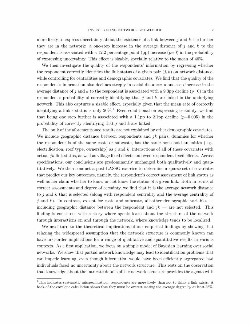
more likely to express uncertainty about the existence of a link between j and k the furtherthey are in the network: a one-step increase in the average distance of j and k to therespondent is associated with a 12.2 percentage point (pp) increase (p=0) in the probabilityof expressing uncertainty. This effect is sizable, specially relative to the mean of 46%.

We then investigate the quality of the respondents’ information by regressing whetherthe respondent correctly identifies the link status of a given pair (j, k) on network distance,while controlling for centralities and demographic covariates. We find that the quality of therespondent’s information also declines steeply in social distance: a one-step increase in theaverage distance of j and k to the respondent is associated with a 9.3pp decline (p=0) in therespondent’s probability of correctly identifying that j and k are linked in the underlyingnetwork. This also captures a sizable effect, especially given that the mean rate of correctlyidentifying a link’s status is only 20%.1 Even conditional on expressing certainty, we findthat being one step further is associated with a 1.1pp to 2.1pp decline (p=0.005) in theprobability of correctly identifying that j and k are linked.

The bulk of the aforementioned results are not explained by other demographic covariates.We include geographic distance between respondents and jk pairs, dummies for whetherthe respondent is of the same caste or subcaste, has the same household amenities (e.g.,electrification, roof type, ownership) as j and k, interactions of all of these covariates withactual jk link status, as well as village fixed effects and even respondent fixed effects. Acrossspecifications, our conclusions are predominantly unchanged both qualitatively and quan-titatively. We then conduct a post-LASSO exercise to determine a sparse set of covariatesthat predict our key outcomes, namely, the respondent’s correct assessment of link status aswell as her claim whether to know or not know the status of a given link. Both in terms ofcorrect assessments and degree of certainty, we find that it is the average network distanceto j and k that is selected (along with respondent centrality and the average centrality ofj and k). In contrast, except for caste and subcaste, all other demographic variables —including geographic distance between the respondent and jk — are not selected. Thisfinding is consistent with a story where agents learn about the structure of the networkthrough interactions on and through the network, where knowledge tends to be localized.

We next turn to the theoretical implications of our empirical findings by showing thatrelaxing the widespread assumption that the network structure is commonly known canhave first-order implications for a range of qualitative and quantitative results in variouscontexts. As a first application, we focus on a simple model of Bayesian learning over socialnetworks. We show that partial network knowledge may lead to identification problems thatcan impede learning, even though information would have been efficiently aggregated hadindividuals faced no uncertainty about the network structure. This rests on the observationthat knowledge about the intricate details of the network structure provides the agents with

1This indicates systematic misspecification: respondents are more likely than not to think a link exists. Aback-of-the envelope calculation shows that they must be overestimating the average degree by at least 38%.


valuable information on how to discern the correlations and redundancies in their neighbors’estimates. Our result thus demonstrates that predictions about learning dynamics may besensitive to the extent and nature of agents’ knowledge about the social network structure.

As a second case study, we illustrate how assuming full network knowledge may leadto biased structural estimates if in fact decision makers face some uncertainty about theunderlying network. We focus on the canonical network interaction game of Ballester et al.(2006) with strategic complementarities. This game, which serves as one of the workhorsemodels for studying strategic network interactions in the literature, allows for simple struc-tural estimates, counterfactuals, and policy prescriptions. We show that uncertainty aboutthe extent of strategic complementarities outside one’s neighborhood results in a system-atic shift in equilibrium actions (relative to the complete information benchmark). Hence,ignoring the possibility of incomplete network knowledge may lead to biased structuralestimates for the degree of complementarities, mis-specified cost-benefit analyses, and po-tentially counterproductive intervention policies (such as identifying “key players” to targetfor interventions).

Finally, we shift our attention to investigating the implications of network knowledge forparameter identification in network formation games. We study a fairly standard economet-ric model of network formation, where the literature has grappled with partial identificationof parameters when agents have complete information about the realization of pairwise pref-erence shocks. However, we show that the equilibrium network in the game with incompleteinformation provides the econometrician with sufficiently rich observations to point-identifyall structural parameters. This result suggests that introducing the (more realistic) as-sumption of incomplete information may transform a model that is fundamentally hard toidentify to a straightforwardly estimable model.

Our work is not the first paper to introduce incomplete information into the above men-tioned contexts. For instance, in the context of social learning, Acemoglu et al. (2011) andLobel and Sadler (2015) allow for randomly generated networks of various kinds. Similarly,papers such as Leung (2015b) and more recently Ridder and Sheng (2017) study networkformation with incomplete information. Our goal here is primarily pedagogical, stronglymotivated by the data. Specifically, our results are meant to clarify the extent to which apotentially unrealistic assumption plays a critical role in a wide variety of applications andhow incorporating partial or lack of network knowledge into fairly standard models can leadto vastly different conclusions.

In addition to the network theory and econometrics literatures discussed above, our paperis related to works in sociology that explore limits to knowledge about others’ traits as wellas perceptions of friendships in networks (Friedkin, 1983; Krackhardt, 1987, 2014). Forinstance, using network data among several departments at the University of Chicago andColumbia University, Friedkin (1983) showed that a respondent i was less likely to knowabout another faculty member j’s current research if the respondent was further from j in


the network. This is in line with findings of Alatas et al. (2016), who show that subjectsare much less likely to know about the wealth status of individuals in their village whoare further away in the network. Relative to these findings, our paper emphasizes thatknowledge about the network itself is similarly limited and localized through the network.2

The rest of the paper is organized as follows. Section 2 describes the setting, data, andsample statistics. Section 3 contains our main empirical findings, where we document hownetwork knowledge relates to the average distance between the respondents and the pairof individuals they are being inquired about. In Section 4, we discuss how our findingsregarding limited network knowledge can be relevant for theoretical, applied, and econo-metric work. Section 5 is a conclusion. All proofs are provided in Appendix A. An onlineappendix contains some additional empirical results.

2. Setting and Data

2.1. Network data collection. We collected data in 75 villages in Karnataka, India,where we have previously worked. The villages span 5 districts around Bangalore wherewe have collected network data in the past: Wave I in 2006 (Banerjee et al., 2013) andWave II in 2012 (Banerjee et al., 2016). In 2012, we collected network data from 89% ofthe over 16,500 households across the 75 villages. These links spanned financial, social, andinformational relationships across 12 dimensions.3 Because such a high share of householdswere surveyed and every household could name links to any other household in the census ineach village, we have 98.8% of all links in the resulting undirected, unweighted network. It isagainst this backdrop that we conducted a subsequent survey to explore network knowledge.

2.2. Knowledge data collection. We conducted a network knowledge questionnaire in2015 by asking 4,554 randomly selected individuals across the 75 villages about networkrelationships between various other individuals in their community. We asked every respon-dent i about network relationships among five distinct pairs j and k. This was stratified inthe following way. We ensured that for each i, one jk pair of each distance 1–1.5, distance2–2.5, distance 3–3.5 distance 4–4.5, and distance 5+ (including unreachables) was selectedin the survey, using our pre-existing network data.4 For each jk pair we asked about theexistence of specific types of network relationships: informational, financial, and social. We

2Krackhardt (1987, 2014) was the first to advocate for collecting data not only about network interactions,but also about others’ perceptions of such interactions. Krackhardt (1987) called these cognitive socialstructures (CSS). Our data could be interpreted as sampling from CSSs in 75 distinct networks.3(1) whose house the respondent visits, (2) who visits her house, (3) kin, (4) whom they socialize with, (5)who gives information when there is a medical need, (6) whom they gives advice to, (7) whom they getadvice from, (8) whom they lend material goods to, (9) whom they borrow material goods from, (10) whomthey borrow money from, (11) whom they lend money to, (12) with whom they go to pray (e.g., at a templeor mosque).4We also asked i about several demographic traits of j and k. These include if they have children, householdsize, main household occupation, monthly income, television ownership, religious details, political disposition,and land ownership.


analyze responses to informational, financial, and social relationships, denoted by index r.5

The resulting object is a graph gr for each r.For every pair jk and relationship type r, we asked i whether gjk,r = 1 or gjk,r = 0.

The respondent could tell us their estimate or tell us that they “Don’t know.” A responseof “Don’t know” could arise for two reasons: either the respondent does not feel certainenough to offer a guess or because the respondent does not know who either j or k are. Therespondent i’s response is therefore hi,jk,r ∈ {1, 0,Don’t Know}.6

Our outcomes of interest are whether the respondent correctly identified link status, i.e.,

yi,jk,r = 1{hi,jk,r = gjk,r},

and whether they were sure enough to offer a guess to being with, i.e.,

DKi,jk,r = 1{hi,jk,r = Don’t Know}.

We are chiefly interested in how yi,jk,r and DKi,jk,r depend on the network distance betweenthe respondent i and the pair jk, conditional on the centralities of the nodes involved anddemographic covariates. While we consider the respondents’ outcomes yi,jk,r = 1{hi,jk,r =gjk,r} for each type of relationship r separately in our regressions, we follow previous workand measure distances and centralities in the union network g = ∪rgr, according to whichtwo agents are assumed to be linked if either agent reports having any of the 12 relationshipdimensions with the other.7

2.3. Sample statistics. Respondent characteristics are summarized in Table 1, Panel A.59% of the respondents were female and the average age in the sample was 42.55. Maleswere typically born in the village (51%) whereas most females married in (only 11% wereborn in the village). The average degree is 19.5 which indicates a sparse network (theaverage number of households in the village is 196). Panel B describe pair characteristics.99% of the pairs belonged to the same connected component as the respondent (i.e., thepair was ‘reachable’), and in our stratified sample, 34% of the time they were linked. Onaverage, the distance from i to jk was 2.13, and 59% of the time they were of the samecaste category. Panel C presents our knowledge survey outcomes. 46% of the time therespondents expressed that they did not know the linking status of the pairs in question.When willing to offer a guess, the respondents correctly identified the linking status of thepair only 20% of the time. Conditional on a link existing, a correct guess was offered 57%

5Specifically, we collapsed some of the Banerjee et al. (2013) survey, leaving us with 3 dimensions: (1) socialinteraction; (2) borrowing/lending of money; (3) giving/receiving advice before an important decision;6Note that even though the subjects report whether or not they believe a given pair of individuals are linked,we do not observe the respondents’ subjective beliefs (i.e., the probability that i assigns to the existence ofa link j and k).7This choice is made to generate the regressors as independent variables because we believe that this generatesthe most natural definition of social distance for our setting. Individuals might learn about a financialrelationships existing in other parts of the network, for example, through financial ties but also throughinformation and social ties.


of the time. This immediately illustrates that respondents systematically overestimated theexistence of a link.8

3. Network Knowledge in the Network

3.1. Knowledge and distance. Our summary statistics in Table 1 already indicate pooraverage knowledge about the network. We next explore how the relative position of nodesinfluences i’s ability to know whether j and k are linked.

To this end, we run core regressions of the following form:

Yi,jk,r = α+ θgjk,r + λr + βnot ·(dist (i, j) + dist (i, k)

2

)· (1− gjk,r)(1)

+ βlink ·(dist (i, j) + dist (i, k)

2

)· gjk,r

+ δnot ·Avg. Centralityjk · (1− gjk,r) + δlink ·Avg. Centralityjk · gjk,r+ γnot · Centralityi · (1− gjk,r) + γlink · Centralityi · gjk,r+X ′i,jkη + εi,jk,r.

Here, Yi,jk,r will either be yi,jk,r, which is a dummy that measures whether i correctlyidentified the link status between j and k, or DKi,jk, which is whether i reported notknowing the status.

Taking for now the case where yi,jk,r is the outcome variable of interest, coefficient θmeasures the difference in the probability of being correct if the link gij,r exists, whereascoefficients λr are relationship type-fixed effects. Coefficient βnot measures the marginalchange in i’s probability of correctly identifying that j and k are not linked when theaverage distance increases by 1, while βlink records how knowledge changes with distancewhen gjk,r = 1.9 Similarly, γnot and γlink measure the marginal effect of being one standarddeviation more central on the probability of being correct when the link does not exist,and that probability when the link does exist. δnot and δlink play the same role but nowlooking at j and k’s centralities. Finally, Xi,jk will include a vector of covariates: averagegeographic distance of i from j and k, their geographic centralities, and dummies for eachof whether i is of the same caste, subcaste, has the same electrification status, has thesame roof type, and has the same ownership status for each of j and k, as well as all thesevariables’ interactions with linked status gjk,r.

8Assuming that each respondent simply offers a response about the existence of a link uniformly at random,a back-of-the-envelope calculation shows that the implied density of the network by our respondents is atleast 37.9% higher than that in the data.9Note that even if respondents have biased guesses about whether links exist when they do not truly know(meaning that their guesses may differ on average from the true rate) this does not affect the test of whetherβnot or βlink is non-zero.


The main results can be seen in the raw data in Panels A–C of Figure 1. Panel A depictsthe share of correct guesses by average network distance between i and the (j, k) pair. Itis immediate to see that the fraction of correct guesses steadily declines in distance downto the unreachable pairs. Panel B illustrates that the share of respondents who do notknow jk’s link status increases across network distance. In Panel C, we condition on havinga view on the link status and then look at whether the guess is correct or not. We seein the raw data that there is a negative correlation between the share of correct guessesand the network distance, meaning that even beyond having a view on the link, there isresidual information which is more accurate for pairs that are on average socially closer tothe respondents.

We can also consider how network knowledge varies with the centralities of j and k. InPanels D–F of Figure 1, we plot the same outcomes of interest, varying average centralities.Here, we see that when j and k are more central, i is more likely to offer a correct guess, isless likely to say that she “Doesn’t know” the link status, and has better information aboutthe existence of a link conditional on having a view. Note that more central j and k aremechanically closer to any arbitrary i, so the relationship between centrality and knowledgeis likely a direct consequence of the relationships in Panels A–C.10

3.1.1. How the likelihood of guessing correctly varies by distance. Table 2 contains our mainnetwork distance results. Panel A looks at how whether i knows jk’s linking status, yi,jk,rdepends on the relative network distances between parties and their centralities. Column 1presents the regression just with the network position variables, column 2 adds the afore-mentioned vector of demographic controls contained in Xi,jk, column 3 adds village fixedeffects, while column 4 also includes respondent fixed effects. Note that the specificationwith respondent fixed effects holds the demographic and network characteristics of the re-spondent fixed, comparing close versus far jk, within respondent.11

We focus on column 1 for exposition. We see that having j and k be on the sameconnected component as i leads to a 6.5pp increase (p=0.001) in the probability of guessingthe status correctly when there is no link. Further, this corresponds to a 54.7pp increase(p=0) in the probability of guessing the status correctly when there is a link.

Next, we study how respondents’ knowledge depends on their network distance to thepair in question. Note that to understand the effect of distance, we need to conditionon reachability through the network, as unreachable individuals have infinite distance tothe respondent. We find that being one step further than j and k on average leads to a1.8pp decline (p=0) in the probability of guessing correctly when there is no link, and moreimportantly a 10.9pp decline (p=0) in the probability of guessing correctly when there isa link. This is a very large effect relative to the mean (19.9%). Furthermore, columns 2–4

10This finding may also help explain why respondents can identify the more central individuals fairly accu-rately (Banerjee et al., 2016).11Online Appendix B presents the same tables with all network covariates.


illustrate that this pattern is robust to a wide range of specifications, clearly indicatingthat the quality of respondent’s information is steeply declining in her network distanceto the pair and is not explained by similarities in demographics such as wealth, caste,electrification, geography, and so on.12

3.1.2. How the likelihood of being certain varies by distance. Note that the correct guessoutcome in Panel A combines both having a view on a given jk relationship and guessingcorrectly about the existence (or not) of that relationship. Panel B of Table 2 focuses onthe first component. The specifications and control sets are the same as in Panel A, butnow our outcome variable is DKi,jk,r, a dummy for whether the respondent declared thatthey “Don’t know” whether j and k are linked.

We find that respondents are considerably more likely to have a view about the networkstructure local to them and are much more uncertain at larger distances. Once again, wefocus on column 1 for exposition, though the results are largely robust to controls andfixed effects. Relative to a mean of 46%, we observe that being reachable leads to a 32.1ppdecline (p=0) in the probability of declaring “Don’t know” when gjk,r = 0 and a 46.6ppdecline (p=0) when gjk,r = 1. These large magnitudes suggests that i has extremely limitedknowledge when j and k are unreachable. Then, conditional on reachability, every extrastep leads to a 10.9pp (or 14.8pp) (p=0) increase in the probability of declaring “Don’tknow” when there is no link (when there is a link) which again is a very large effect relativeto the mean.

Next, we further decompose the “Don’t know” response into its two components — notknowing that either j or k exist and knowing of j and k, but not having a view on theirrelationship. We explore this decomposition in Table 3. Columns 1 and 2 consider whetherrespondent i knows of both j and k as a function of distance and reachability. Note thatthis variable is defined at the (i, j, k) level and does not vary across relationship types. Wetherefore collapse the data in columns 1 and 2 to that level. First note that i knows ofboth j and k only 64% of the time. This means that approximately three-fourths of the“Don’t know” responses come from not knowing anything about one or both of the nodesin question. Unsurprisingly, the patterns of knowledge as a function of reachability anddistance look very similar to those in Table 2, Panel B. In columns 3 and 4, we ask whetherconditional on knowing that j and k exist, there is a residual relationship between DKi,jk,r

and the distance between i and jk. We find that all of the qualitative patterns survive in thisconditional regression: reachability is correlated with a lower likelihood of “Don’t know”,while larger social distances make a “Don’t know” response more likely. For example, when

12We note that adding controls does reduce the magnitude of the coefficient on reachability when there is alink. The other three coefficients are stable across specifications.


gjk,r = 1, moving jk one step further from i is associated with a 4.5pp increase (p=0) inDKi,jk,r.13

3.1.3. Is there residual information conditional on a degree of certainty? Having establishedthat the likelihood that a guess is correct and the likelihood of having a view both decline indistance, we now study whether these results are solely driven by respondents’ uncertainty(“Don’t know”) or whether within a certainty bin, i’s responses are more accurate whenjk are socially closer. Table 2, Panel C presents the results of regressions that conditionon having a view about the relationship. The control sets across columns are the same asthose used in Panels A and B.

We first note that these regressions condition on individuals i, pairs jk, and relationshipdimensions r for which respondent i claims to know about the relationship status. Giventhat we just showed that having a view is also a function of distance, this creates a censoringproblem that could lead to bias in the estimated relationship of interest. We believe thatthe most logical form of bias should make it harder to detect a negative relationship betweensocial distance and bias. This would be the case if i were more likely to have an opinionabout far jk pairs who were nonetheless “closer” on unobservables and if those unobservablesalso corresponded to a higher likelihood of a correct guess.

Keeping that caveat in mind, we do find evidence that distance is correlated with makinga correct guess, even conditioning on DKi,jk,r = 0. We again find that being 1 step higher interms of average distance to j and k leads to a decrease of between 1.1 and 2.1pp (p=0.005)in the probability of guessing correctly when there is a link between jk. However, there isno detectable pattern in distance when gjk,r = 0.

That network distance still predicts accuracy, even conditional on having a view, isconsistent with the idea that simply knowing something about j and k does not drivethe entire relationship identified in Table 2, Panel A. Instead, a systematic bias developsmore strongly outside the local radius.

3.2. What best predicts network knowledge? Our findings thus far illustrate thatnetwork knowledge is systematically predicted by and related to the social distance betweenrespondent i and the pair jk in question. We also demonstrated that this correlation is notaffected by the inclusion of numerous controls including amenities, caste, geography, villagefixed effects, and respondent fixed effects.

We now ask something stronger: out of all the variables we have at our disposal, what bestpredicts network knowledge? For example, it may be geography, because people observethose who live nearby interacting with others, even if they are not themselves linked. Orit may be the network itself, because people interact on and through the network, so one

13We note that the regressions in columns 3 and 4 control on an outcome that we have already shown to becorrelated with distance. See Section 3.1.3 below for a discussion of the likely bias.


is more likely to know about relationships among one’s friends or friends of friends ratherthan someone who is an effective stranger.

To this end, we conduct a post-LASSO procedure (Belloni and Chernozhukov (2013)and Belloni, Chernozhukov, and Hansen (2014b,a)) by regressing the outcome, whetheri knows link jk exists or not (or how certain i is), on the network variables and all thedemographic variables as before. Since this procedure penalizes putting in many parameterswith the aim of selecting a sparse subset of covariates, it may wind up picking a minimalmodel that excludes network variables altogether. Alternatively, it may include network-based variables, viewing them as more predictive than any of our demographic covariates.Note that since LASSO is a shrinkage estimator, the post-LASSO procedure ensures thatconsistent estimates are being used.

Table 4 presents the results of this exercise. Column 1 contains the estimates when theoutcome is whether the respondent’s guess is correct (yi,jk,r). Three core network variablesare selected: the distance to the pair when there is no link, centrality of i when jk are linked,and the average centrality of the pair jk when they are linked. As we have mentioned before,the centralities of j and k are highly (negatively) correlated with average distances withan arbitrary i. Additionally (but omitted from the display), the following demographicsare selected: dummies for whether i and j, i and k, and j and k are of the same caste,subcaste, have the same occupation, house ownership status, roof type, and electrificationstatus.14 In column 2 we predict the responses DKi,jk,r of the agent. We find that thedistance is selected both when gjk,r = 0 and gjk,r = 1. Being one step further correspondsto a 8.99pp (or a 19.6%) (p=0) increase in the probability of declaring “Don’t know”. Twoother network measures are selected here: the centrality of the respondent when gjk,r = 1and the average centralities of jk when gjk,r = 0. In this case, a smaller set of demographicsis selected: average geographic distance between j and k, and all variables relating to thecastes and subcastes of i, j, and k.15 Note that in either case geographic distance fromrespondent to respondees or geographic centralities are not selected.

This suggests that an important set of predictive variables in terms of network knowledgeor certainty about this knowledge consists of distance in the network from the respondent,how central the respondent is, and how central those in consideration are. These variablesare selected by a post-LASSO procedure in a large horserace against a number of alter-natives, including geographic variables. This is consistent with a story where people learnabout their social structure by exploring/interacting through their social structure.

1423 village fixed effects and 1 dimension fixed effect are also selected.15In addition, one occupation variable is selected along with 44 village fixed effects.


4. Importance of assumptions on network knowledge

In this section, we discuss how our findings regarding limited network knowledge can berelevant for theoretical, applied, and econometric work. Assuming that agents have completeinformation about the underlying network is an oft-used assumption in the literature (withapplications ranging from social learning and peer effects to network formation games). Inwhat follows, we demonstrate how such an assumption (or lack thereof) can have first-orderimplications for a range of qualitative and quantitative results in various contexts.

4.1. Social learning. As our starting point, we explore the implications of network un-certainty in the context of learning over social networks. Many models of Bayesian sociallearning assume that agents have complete knowledge about the social network structure.16

In what follows we use a simple framework to illustrate that relaxing the assumption of fullnetwork knowledge may lead to identification problems that can serve as impediments tolearning, even when agents have access to enough information to uncover the state. Cru-cially, we also show that these identification problems do not arise when individuals face nouncertainty about the network.

Consider a collection of n+ 1 individuals, denoted by {0, 1, . . . , n}, who wish to estimatean unknown state of the world θ ∈ R. Each agent i receives a noisy private signal si = θ+εi

about the underlying state, where the error terms εi ∼ N (0, σ2) are drawn independentlyacross agents. Prior to observing their private signals, all agents share an (improper)uniform prior belief about the state.

In addition to her private signals, each agent observes the point estimates of a subsetof other individuals, whom we refer to as her neighbors. More specifically, we assumethat agents are located on a directed, acyclic network that determines the patterns ofobservations: agent i can observe agent j’s point estimate ωj about the state if and only ifthere is a directed link from agent j to agent i.17

We represent the potential lack of knowledge about the social network structure byassuming that agent 0 is ex ante uncertain about the patterns of connections among otherindividuals. More specifically, we assume that the underlying network is drawn randomlyfrom the set G = {g1,g2} with probabilities p1 and p2 = 1− p1, respectively, where

gi = {ij : j 6= 1, 2} ∪ {j0 : j 6= 0}

16This includes both sequential learning models such as Banerjee (1992), Bikhchandani, Hirshleifer, andWelch (1992), and Smith and Sørensen (2000) as well as models of repeated network interactions such asMossel, Sly, and Tamuz (2015) and Mossel, Olsman, and Tamuz (2016).17A directed network is said to be acyclic if it contains no directed cycles. The assumption that the networkis acyclic ensures that information flows are unidirectional. This assumption is also equivalent to imposingan exogenous sequence of timing for agents’ observations and assuming that each agent i can only observethe point estimates of a subset of her predecessors, as in Banerjee (1992) and Acemoglu, Dahleh, Lobel, andOzdaglar (2011), among others.


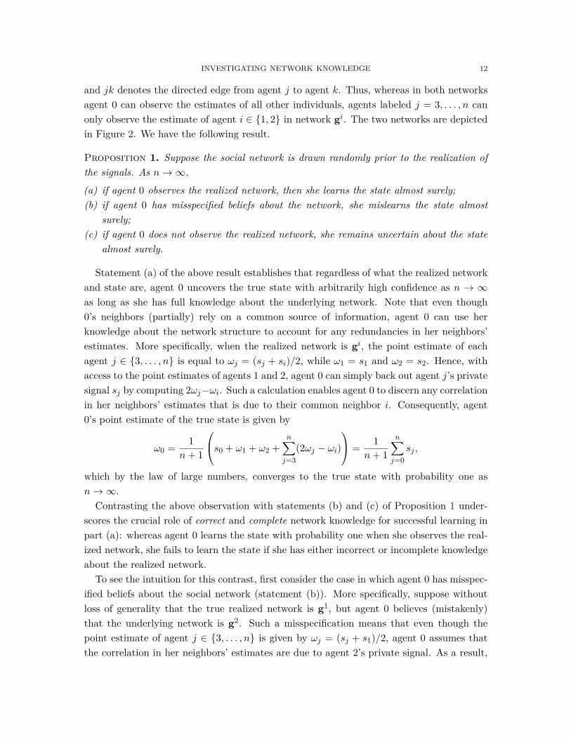
and jk denotes the directed edge from agent j to agent k. Thus, whereas in both networksagent 0 can observe the estimates of all other individuals, agents labeled j = 3, . . . , n canonly observe the estimate of agent i ∈ {1, 2} in network gi. The two networks are depictedin Figure 2. We have the following result.

Proposition 1. Suppose the social network is drawn randomly prior to the realization ofthe signals. As n→∞,

(a) if agent 0 observes the realized network, then she learns the state almost surely;(b) if agent 0 has misspecified beliefs about the network, she mislearns the state almost

surely;(c) if agent 0 does not observe the realized network, she remains uncertain about the state

almost surely.

Statement (a) of the above result establishes that regardless of what the realized networkand state are, agent 0 uncovers the true state with arbitrarily high confidence as n → ∞as long as she has full knowledge about the underlying network. Note that even though0’s neighbors (partially) rely on a common source of information, agent 0 can use herknowledge about the network structure to account for any redundancies in her neighbors’estimates. More specifically, when the realized network is gi, the point estimate of eachagent j ∈ {3, . . . , n} is equal to ωj = (sj + si)/2, while ω1 = s1 and ω2 = s2. Hence, withaccess to the point estimates of agents 1 and 2, agent 0 can simply back out agent j’s privatesignal sj by computing 2ωj−ωi. Such a calculation enables agent 0 to discern any correlationin her neighbors’ estimates that is due to their common neighbor i. Consequently, agent0’s point estimate of the true state is given by

ω0 = 1n+ 1

s0 + ω1 + ω2 +n∑j=3

(2ωj − ωi)

= 1n+ 1

n∑j=0

sj ,

which by the law of large numbers, converges to the true state with probability one asn→∞.

Contrasting the above observation with statements (b) and (c) of Proposition 1 under-scores the crucial role of correct and complete network knowledge for successful learning inpart (a): whereas agent 0 learns the state with probability one when she observes the real-ized network, she fails to learn the state if she has either incorrect or incomplete knowledgeabout the realized network.

To see the intuition for this contrast, first consider the case in which agent 0 has misspec-ified beliefs about the social network (statement (b)). More specifically, suppose withoutloss of generality that the true realized network is g1, but agent 0 believes (mistakenly)that the underlying network is g2. Such a misspecification means that even though thepoint estimate of agent j ∈ {3, . . . , n} is given by ωj = (sj + s1)/2, agent 0 assumes thatthe correlation in her neighbors’ estimates are due to agent 2’s private signal. As a result,


agent 0’s point estimate is given by

ω0 = 1n+ 1

s0 + ω1 + ω2 +n∑j=3

(2ωj − ω2)

= 1n+ 1

(n− 2)(s1 − s2) +n∑j=0

sj

,which converges to θ + s1 − s2 with probability one, whenever the true state is θ. In otherwords, agent 0’s misspecified belief about the network structure manifests itself as a bias inher estimate about the state.

Finally, part (c) of Proposition 1 illustrates that uncertainty about the network structurecan create an identification problem that would serve as an impediment to learning. In thecontext of the above example, no matter how many neighbors agent 0 has, she can onlylearn the state by properly accounting for the redundancies and patterns of correlations inher neighbors’ estimates. Yet, uncertainty about the identity of her neighbors’ neighborsmeans that agent 0 cannot identify the source of such redundancies. More specifically, whenthe true state and the realized network are θ and g1, respectively, agent 0 has no way ofdistinguishing whether the underlying state-network pair is (θ,g1) or (θ+ s1− s2,g2), evenas n→∞. This is despite the fact that she can hold and update beliefs not only about thestate but also about the underlying network structure.18

Taken together, Proposition 1 illustrates that incorrect or incomplete knowledge aboutthe social network can undermine information aggregation, even in fairly simple environ-ments that would have otherwise led to learning. This observation, alongside our empiricalfindings in Section 3, suggests that Bayesian models that allow for uncertainty about thenetwork structure (such as Lobel and Sadler (2015)) as well as behavioral models (suchas DeGroot (1974), Eyster and Rabin (2014), and Li and Tan (2017)) that assume agentscannot fully account for how the network structure shapes their observations may be usefuland important starting points for applied work to focus on.

4.2. Network interactions and peer effects. We next focus on network peer effectgames and illustrate how assuming full network knowledge may lead to biased structuralestimates when in fact agents face uncertainty about the underlying network.

To this end, we focus on the canonical network interaction model of Ballester, Calvo-Armengol, and Zenou (2006). Besides their widespread use, models that build off thislinear-quadratic framework lend themselves to readily obtainable structural estimates, aswell as counterfactual and policy analyses (such as which “key” players to target with anintervention). Applications include peer effects in education (Calvo-Armengol, Patacchini,and Zenou, 2009), local consumption externalities (Candogan, Bimpikis, and Ozdaglar,

18In this sense, our result on the role of network uncertainty is similar to Acemoglu, Chernozhukov, andYildiz (2016), who argue that uncertainty about the signal generating process can result in an identificationproblem for a single Bayesian agent in isolation, as the same long-run frequency of signals may be consistentwith multiple states.


2012), research collaboration among firms (Goyal and Moraga-Gonzalez, 2001), among nu-merous others.

The basic setup is an n-player game in which agents’ payoffs are given by

ui(x1, . . . , xn) = xiθi −12x

2i + α

∑j 6=i

gijxixj ,

where xi denotes the action (say, effort) of agent i, gij regulates the strength of strategiccomplementarities between i and j, and parameters α ∈ [0, 1) and θi > 0 are commonknowledge among all agents.

As is common in the literature, pairwise interactions can be represented by a directedand weighted network g = [gij ], with the convention that gii = 0 for all i. In a departurefrom the rest of the literature, however, we assume that this interaction network is drawnrandomly prior to the start of the game. More specifically, we assume that for any pair ofagents i 6= j, the weight gij is drawn independently from the rest of the weights accordingto a non-degenerate probability distribution with density fij . Throughout, we assume that∑j 6=i max supp(fij) ≤ 1 for all agents i.19

We consider two variants of the above game. In what we call the complete informationbenchmark, we assume that the realized network g is observed by all agents prior to makingtheir decisions. Therefore, ex post, our complete information benchmark coincides with thecanonical model of Ballester, Calvo-Armengol, and Zenou (2006). On the other hand,under the incomplete information variant of the game, we assume that each agent i canonly observe the set of weights {gij : j 6= i} in her neighborhood. Hence, in contrast to thecomplete information benchmark, agents choose their actions with no knowledge about thestrength of strategic complementarities among other agents. We have the following result:

Proposition 2. The vectors of equilibrium actions under the complete and incompleteinformation variants of the game are given by

xcom = (I − αg)−1θ(2)

xinc =(I + αg(I − αE[g])−1

)θ,(3)

respectively. Furthermore, E[xinci ] < E[xcom

i ] for all agents i.

The above result establishes that equilibrium actions are sensitive to whether agents havefull knowledge about the patterns of interactions in the network. More importantly however,Proposition 2 also illustrates that uncertainty about the network structure results in asystematic shift in equilibrium actions: each agent’s action in the incomplete informationgame is in expectation less than her action in the complete information benchmark.

What this means, practically, is that estimates of θ and α obtained under the assumptionof complete information may be biased if agents are in fact uncertain about the network19This restriction on the support of the distributions is meant to guarantee that the matrix I − αg isinvertible with probability one.


structure. Such biases can in turn substantially affect not only counterfactuals but alsopolicy prescriptions by potentially impacting (i) cost-benefit assessments, (ii) the predictedextent of externalities, and (iii) the relative network centralities of various agents; a statisticthat is central to policy prescriptions in this literature.

4.3. Identification in network formation games. We conclude this section by inves-tigating the implications of incomplete network knowledge for identification of structuralparameters in network formation games. As our main result, we show that introducingthe (arguably more realistic) assumption of incomplete information may transform a modelthat is fundamentally hard to identify to a straightforwardly estimable model.

Consider a simultaneous-move game of network formation with n players, indexed {1, . . . , n}.Each agent i is endowed with some attribute zi ∈ {a, b}. These attributes, which are com-mon knowledge among all agents and are observable to the econometrician, may representagents’ gender, caste, race, or other characteristics. Throughout, we use λ to denote thefraction of agents with attribute a.

Agents draw utilities by forming direct and indirect links with other individuals. Morespecifically, the utility function of agent i is given by

ui(g, z, εi) =∑j 6=i

gij(α− εij) + β∑j 6=i

gij1{zj = zi}+ γ

1n− 1

∑j 6=i

∑k 6=i,j

gijgjk

,(4)

where g denotes the undirected, unweighted network of linkages (with gij = 1 if i and j arelinked and gij = 0 otherwise), z = (z1, . . . , zn) denotes the vector of population attributes,and εij is a preference shock that determines agent i’s idiosyncratic cost of establishing alink to agent j. Throughout, we assume that preference shocks are drawn independentlyfrom a common probability distribution F (·) with a continuous density and full supportover R.

The first two terms on the right-hand side of (4) capture the (net) direct utility of forminglinkages: agent i obtains a net marginal utility of α − εij of forming a direct link to agentj, with an additional marginal benefit of β if the two agents have identical attributes. Onthe other hand, the third term on the right-hand side of (4) allows for the possibility thatindirect connections can also be payoff relevant. For example, when γ > 0, agent i draws abenefit if any of her neighbors form links with other individuals.20

Players simultaneously announce the set of agents they wish to link to, with links formedby mutual consent. Formally, each player i chooses the action xij ∈ {0, 1} indicating

20As in Sheng (2016) and Mele (2017), the specification in (4) assumes that the indirect benefits of forminglinks are proportional to the number of connections of i’s neighbors. An alternative specification is to assumethat indirect benefits only depend on the number of distinct connections of i’s neighbors, as in de Paula,Richards-Shubik, and Tamer (2018). Our choice of the specification in (4) is made to simplify the analysis.However, our main result on the relationship between network knowledge and the identifiability of structuralparameters holds for a broader class of specifications.


whether she wishes to form a link with agent j. The undirected link (i, j) is then formed ifboth parties agree, i.e., gij = xijxji.

The econometrician is interested in estimating the structural parameters α, β, and γ

in (4) while only observing the equilibrium network g. The literature typically assumesthat the realizations of preference shocks εij are common knowledge among the agentsand that agents are in a pairwise stable network (de Paula, Richards-Shubik, and Tamer,2018; Leung, 2015a; Menzel, 2017; Sheng, 2016). This observability assumption means thatagents’ link formation decisions xij ∈ {0, 1} can be contingent on the realization of allpairwise preference shocks.

The fact that network formation games of complete information tend to pose a challengefor identification has been at the forefront of the literature. To overcome this issue, theliterature has resorted to imposing subsequent stronger assumptions on agents’ payoffs, thenumber of preference shocks, or the network formation process (see, e.g., de Paula et al.(2018); Leung (2015a); Menzel (2017); Sheng (2016)).

In a departure from the literature, we assume that preference shocks are only locallyobservable: the realization of agent i’s preference shocks εi = (εi1, . . . , εin) are i’s privateinformation and hence are unobservable to all other agents. Given the incomplete informa-tion nature of this specification, we focus on (symmetric monotone) Bayes-Nash equilibriumas our solution concept, according to which each agent i chooses the action xij = 1 if therealized preference shock εij falls below some given threshold that only depends on i andj’s attributes.

Before presenting our result, we remark that the notion of incomplete information inthis context is slightly different from those in Subsections 4.1 and 4.2. Whereas our earlierexamples focused on the observability (or lack thereof) of the network structure itself, theincomplete information variant of the network formation game above requires the agents tobe uncertain about the realizations of the underlying pairwise preference shocks.

Proposition 3. Suppose the econometrician observes the realized network but not the real-ization of the preference shocks and λ 6= 1/2. If preference shocks are only locally observable,structural parameters α, β, and γ are point-identified.

The proposition illustrates that relaxing the complete information assumption leads toa diametrically opposite result of that in the literature: observing the pattern of linkagesprovides the analyst with sufficiently rich information to point-identify all structural pa-rameters. This contrast is driven by the fact that when players have limited information,they are unable to condition their decisions on the fine details of the entire set of realizedshocks {εij}, leading to coarser linking strategies and hence facilitating identification. Thisillustrates that imposing the simple and — in view of our empirical findings in Section 3 —more realistic assumption of incomplete information transforms a model that is fundamen-tally hard to identify to a realistic and straightforwardly estimable model, without changing


the payoffs, imposing specific link formation dynamics, or restricting the number or typesof links that can be formed.

5. Conclusion

We present a new set of stylized facts about the extent to which individuals are informedabout network relationships in their own communities. We collected survey data in 75communities where we had already documented the full network structure across a numberof dimensions. We find that network knowledge is low and localized: respondents oftendo not know linking statuses among others in their village and that network knowledgedecays steeply in network distance to the pair. These patterns are robust to the inclusion ofnumerous covariates (e.g., amenities, caste, geography) and are consistent with individualslearning about the social network through the network itself.

Our findings are at odds with many commonly-used modeling techniques in network eco-nomics across a range of questions and applications. Moving from a complete informationframework to an incomplete information framework can lead to changes in the behavior ofagents in the models and, thus different predictions or equilibria, thereby affecting qual-itative conclusions and structural estimates. Further, we show that typical econometricmodels of network formation have the features that moving to the more realistic assump-tion of incomplete information may make parameters identifiable whereas under the lessrealistic assumption of complete information, parameters may not be identifiable or onlypartially identifiable. We are certainly not the first to explore incomplete information inany of these cases. However, we view our examples playing a pedagogical role, pointingout how this ubiquitous assumption in the literature, inconsistent with the data, may affectwidespread conclusions.

Taken together, our empirical and theoretical results suggest that the complete informa-tion benchmark is not an accurate view of the world for the setting we study, and moreover,is not always a benign assumption. Rather, incorporating incomplete network informationmay yield theoretical predictions that better match the behaviors of agents in real-worldnetworks. Incomplete information may also play a simplifying role in the theory, both yield-ing a smaller set of equilibria in games of cooperation and also leading to smaller identifiedsets in network econometric models.


References

Acemoglu, D., V. Chernozhukov, and M. Yildiz (2016): “Fragility of asymptoticagreement under Bayesian learning,” Theoretical Economics, 11, 187–225. 18

Acemoglu, D., M. A. Dahleh, I. Lobel, and A. Ozdaglar (2011): “Bayesian learningin social networks,” The Review of Economic Studies, 78, 1201–1236. 1, 17

Alatas, V., A. Banerjee, A. G. Chandrasekhar, R. Hanna, and B. A. Olken(2016): “Network structure and the aggregation of information: Theory and evidencefrom Indonesia,” American Economic Review, 106, 1663–1704. 1

Ballester, C., A. Calvo-Armengol, and Y. Zenou (2006): “Who’s who in networks.Wanted: The key player,” Econometrica, 74, 1403–1417. 1, 4.2

Banerjee, A., A. G. Chandrasekhar, E. Duflo, and M. O. Jackson (2013): “Thediffusion of microfinance,” Science, 341, 1236498. 2.1, 5

——— (2016): “Gossip: Identifying Central Individuals in a Social Network,” NBER Work-ing Paper No. 20422. 1, 2.1, 10

Banerjee, A. V. (1992): “A simple model of herd behavior,” The Quarterly Journal ofEconomics, 107, 797–817. 1, 16, 17

Belloni, A. and V. Chernozhukov (2013): “Least squares after model selection inhigh-dimensional sparse models,” Bernoulli, 19, 521–547. 3.2

Belloni, A., V. Chernozhukov, and C. Hansen (2014a): “High-dimensional methodsand inference on structural and treatment effects,” The Journal of Economic Perspectives,29–50. 3.2

——— (2014b): “Inference on treatment effects after selection among high-dimensionalcontrols,” The Review of Economic Studies, 81, 608–650. 3.2

Bikhchandani, S., D. Hirshleifer, and I. Welch (1992): “A theory of fads, fashion,custom, and cultural change as information cascades,” Journal of Political Economy, 100,992–1026. 16

Calvo-Armengol, A., E. Patacchini, and Y. Zenou (2009): “Peer effects and socialnetworks in education,” Review of Economic Studies, 76, 1239–1267. 1, 4.2

Candogan, O., K. Bimpikis, and A. Ozdaglar (2012): “Optimal pricing in networkswith externalities,” Operations Research, 60, 883–905. 1, 4.2

de Paula, A., S. Richards-Shubik, and E. Tamer (2018): “Identifying preferences innetworks with bounded degree,” Econometrica, 86, 263–288. 1, 20, 4.3

DeGroot, M. H. (1974): “Reaching a consensus,” Journal of the American StatisticalAssociation, 69, 118–121. 4.1

Eyster, E. and M. Rabin (2014): “Extensive imitation is irrational and harmful,” TheQuarterly Journal of Economics, 129, 1861–1898. 4.1

Friedkin, N. E. (1983): “Horizons of observability and limits of informal control in orga-nizations,” Social Forces, 62, 54–77. 1


Goyal, S. and J. L. Moraga-Gonzalez (2001): “R&D networks,” The RAND Journalof Economics, 32, 686–707. 4.2

Krackhardt, D. (1987): “Cognitive social structures,” Social networks, 9, 109–134. 1, 2——— (2014): “A preliminary look at accuracy in egonets,” in Contemporary Perspectives

on Organizational Social Networks, Emerald Group Publishing Limited, 277–293. 1, 2Leung, M. P. (2015a): “A random-field approach to inference in large models of network

formation,” Available at SSRN. 1, 4.3——— (2015b): “Two-step estimation of network-formation models with incomplete infor-

mation,” Journal of Econometrics, 188, 182–195. 1Li, W. and X. Tan (2017): “Learning in local networks,” Working paper. 4.1Lobel, I. and E. Sadler (2015): “Information diffusion in networks through social learn-

ing,” Theoretical Economics, 10, 807–851. 1, 4.1Mele, A. (2017): “A structural model of dense network formation,” Econometrica, 85,

825–850. 20Menzel, K. (2017): “Strategic network formation with many agents,” Working paper. 1,

4.3Mossel, E., N. Olsman, and O. Tamuz (2016): “Efficient Bayesian learning in social

networks with Gaussian estimators,” in Annual Allerton Conference on Communication,Control, and Computing, Allerton House, Illinois, 425–432. 16

Mossel, E., A. Sly, and O. Tamuz (2015): “Strategic learning and the topology of socialnetworks,” Econometrica, 83, 1755–1794. 1, 16

Ridder, G. and S. Sheng (2017): “Estimation of large network formation games,” Work-ing paper. 1

Sheng, S. (2016): “A structural econometric analysis of network formation games,” Work-ing paper. 1, 20, 4.3

Smith, L. and P. N. Sørensen (2000): “Pathological outcomes of observational learning,”Econometrica, 68, 371–398. 1, 16


Figures

0.1

.2.3

.4Sh

are

of c

orre

ct g

uess

es

1 1.5 2 2.5 3 4 5 Unreachable

(a) Share of CorrectGuesses by Distance

0.1

.2.3

.4.5

.6.7

.8Sh

are

of d

on't

know

s

1 1.5 2 2.5 3 4 5 Unreachable

(b) Share of Don’tKnows by Distance

0.1

.2.3

.4.5

Shar

e of

cor

rect

gue

sses

1 1.5 2 2.5 3 4 5 Unreachable

(c) Share of CorrectGuesses by Distance,conditional on claimingto know

0.1

.2.3

Shar

e of

cor

rect

gue

sses

<-1 (-1,-0.5] (-0.5,0] (0,0.5] (0.5,1] >1

(d) Share of CorrectGuesses by Centralityof jk

0.1

.2.3

.4.5

.6Sh

are

of d

on't

know

s

<-1 (-1,-0.5] (-0.5,0] (0,0.5] (0.5,1] >1

(e) Share of Don’tKnows by Centrality ofjk

0.1

.2.3

.4.5

Shar

e of

cor

rect

gue

sses

<-1 (-1,-0.5] (-0.5,0] (0,0.5] (0.5,1] >1

(f) Share of CorrectGuesses by Centralityof jk, conditional onclaiming to know

Figure 1. Panels A–C depict raw shares of correct guesses and declaringthat the respondent doesn’t know by distance. Panels D–F show the sameby average centrality of j and k (standardized).

0

n43

21

(a)

0

n43

21

(b)

Figure 2. Networks g1 (left) and g2 (right). Arrows indicate the direction overwhich information can flow from one agent to another.


Tables

Table 1. Sample Statistics

Panel A: Respondent Characteristicsmean obs

Female 0.59 4838Age 42.55 4838General or OBC 0.65 4838Born in the village 0.27 4838Born in the village (female) 0.11 2854Born in the village (male) 0.51 1984Degree 19.51 4838Eigenvector centrality 0.07 4838

Panel B: Pair Characteristicsmean obs

j,k Reachable 0.99 21861j,k Linked 0.34 21861Avg. distance to j,k 2.13 21861Avg. degree centrality of j,k 18.68 21861Avg. eigenvector centrality of j,k 0.06 21861Same caste category j,k 0.59 21834Same subcaste j,k 0.44 21818

Panel C: Knowledgemean obs

Correct guess 0.20 66810Correct guess (j,k not linked) 0.07 43884Correct guess (j,k linked) 0.57 22926Don’t know 0.46 66810


Table 2. Network Knowledge as a function of Distance and Centralities

Panel A: Correct guesses (including don’t knows as wrong guesses)(1) (2) (3) (4)

VARIABLES Correct guess Correct guess Correct guess Correct guess

1{Reachable j,k, Not linked j,k} 0.0647 0.0639 0.0549 0.0420(0.0196) (0.0192) (0.0194) (0.0224)[0.001] [0.001] [0.006] [0.065]

1{Reachable j,k, Linked j,k} 0.547 0.147 0.122 0.174(0.0227) (0.112) (0.108) (0.142)[0.000] [0.193] [0.261] [0.224]

Avg. distance to j,k, Not linked j,k -0.0177 -0.0153 -0.0115 -0.0133(0.00398) (0.00389) (0.00400) (0.00437)

[0.000] [0.000] [0.005] [0.003]Avg. distance to j,k, Linked j,k -0.109 -0.0943 -0.0920 -0.0925

(0.00729) (0.00656) (0.00607) (0.00673)[0.000] [0.000] [0.000] [0.000]

Observations 66,810 66,810 66,810 66,810Depvar mean 0.199 0.199 0.199 0.199

Panel B: Don’t knows(1) (2) (3) (4)

VARIABLES Don’t know Don’t know Don’t know Don’t know

1{Reachable j,k, Not linked j,k} -0.321 -0.271 -0.246 -0.253(0.0377) (0.0362) (0.0288) (0.0335)[0.000] [0.000] [0.000] [0.000]

1{Reachable j,k, Linked j,k} -0.466 -0.355 -0.244 -0.228(0.0381) (0.153) (0.163) (0.216)[0.000] [0.023] [0.139] [0.293]

Avg. distance to j,k, Not linked j,k 0.109 0.0933 0.0854 0.0811(0.00866) (0.00939) (0.00653) (0.00686)

[0.000] [0.000] [0.000] [0.000]Avg. distance to j,k, Linked j,k 0.148 0.123 0.118 0.122

(0.00873) (0.00788) (0.00784) (0.00887)[0.000] [0.000] [0.000] [0.000]

Observations 66,810 66,810 66,810 66,810Depvar mean 0.463 0.463 0.463 0.463

Panel C: Correct guesses (conditional on sure guesses only)(1) (2) (3) (4)

VARIABLES Correct guess Correct guess Correct guess Correct guess

1{Reachable j,k, Not linked j,k} 0.00979 0.0348 0.0327 -0.00996(0.0432) (0.0424) (0.0368) (0.0484)[0.821] [0.414] [0.378] [0.837]

1{Reachable j,k, Linked j,k} 0.534 -0.158 -0.101 0.108(0.0423) (0.108) (0.127) (0.359)[0.000] [0.148] [0.427] [0.764]



(0.00697) (0.00711) (0.00727) (0.00924)[0.008] [0.005] [0.017] [0.239]

Observations 35,909 35,909 35,909 35,909Depvar mean 0.371 0.371 0.371 0.371Notes: Standard errors (clustered at village level) are reported in parentheses. p-values are re-ported in brackets. All columns control for eigenvector centrality of i and avg. eigenvector cen-trality of j,k, when gjk is 1 and 0. All columns also include dimension fixed-effects. Columns (2),(3) and (4) control for demographic covariates. Demographic controls include average geographicdistance of i from j and k and dummies for each of whether i is of the same caste, subcaste, hasthe same electrification status, has the same roof type, has the same number of rooms, and hasthe same house ownership status for each of j and k, when gjk is 1 and 0. They also include theabove-mentioned dummies for when j and k have the same demographic traits. Columns (3) and(4) include village and respondent fixed-effects, respectively.


Table 3. Network Knowledge, conditional on knowing j,k, as a function ofDistance and Centralities

(1) (2) (3) (4)VARIABLES Know pair Know pair Don’t know Don’t know

1{Reachable j,k, Not linked j,k} 0.337 0.289 -0.0671 -0.0490(0.0393) (0.0389) (0.0355) (0.0337)[0.000] [0.000] [0.063] [0.150]

1{Reachable j,k, Linked j,k} 0.446 0.349 -0.122 -0.0548(0.0395) (0.174) (0.0338) (0.0672)[0.000] [0.049] [0.001] [0.418]

Avg. distance to j,k, Not linked j,k -0.109 -0.0959 0.0323 0.0229(0.00923) (0.00975) (0.00736) (0.00728)

[0.000] [0.000] [0.000] [0.002]Avg. distance to j,k, Linked j,k -0.137 -0.116 0.0447 0.0349

(0.00948) (0.00834) (0.00641) (0.00738)[0.000] [0.000] [0.000] [0.000]

Observations 22,270 22,270 42,750 42,750Know pair only X XDepvar mean 0.640 0.640 0.160 0.160Number of (i, jk)s 14250 14250Notes: Standard errors (clustered at village level) are reported in parentheses. p-valuesare reported in brackets. All columns control for eigenvector centrality of i and avg.eigenvector centrality of j,k, when gjk is 1 and 0. Columns (3) and (4) include dimen-sion fixed-effects. Columns (2) and (4) control for demographic covariates. Demographiccontrols include average geographic distance of i from j and k and dummies for each ofwhether i is of the same caste, subcaste, has the same electrification status, has the sameroof type, has the same number of rooms, and has the same house ownership status foreach of j and k, when gjk is 1 and 0. They also include the above-mentioned dummiesfor when j and k have the same demographic traits.


Table 4. Post-LASSO Estimates

(1) (2)VARIABLES Correct guess Don’t know

Avg. distance to j,k, Not linked j,k -0.0269 0.105(0.00367) (0.00603)

[0.000] [0.000]Avg. distance to j,k, Linked j,k 0.0899

(0.00554)[0.000]

Centrality (std.) of i, Linked j,k 0.0134 -0.0125(0.00582) (0.00560)

[0.024] [0.029]Avg. centrality (std.) of j,k, Not linked j,k -0.00211

(0.00692)[0.761]

Avg. centrality (std.) of j,k, Linked j,k 0.0121(0.00520)

[0.022]

Observations 57,597 63,558Reachable pairs only X XLASSO-selected Demographic controls X XLASSO-selected Village FE X XDepvar mean 0.204 0.459Notes: Standard errors (clustered at village level) are reported in paren-theses. p-values are reported in brackets. Demographic controls includeaverage geographic distance of i from j and k and dummies for each ofwhether i is of the same caste, subcaste, has the same electrification sta-tus, has the same roof type, has the same number of rooms, and has thesame house ownership status for each of j and k, when gjk is 1 and 0.They also include the above-mentioned dummies for when j and k havethe same demographic traits. Post-LASSO procedure used with optimalpenalty parameter to select variables.


Appendix A. Proofs

Proof of Proposition 1.

Proof of part (a). Throughout, let ωn = (ω1, . . . , ωn), where ωi denotes the point estimatesof agent i. Without loss of generality, suppose the true underlying state and the realizednetwork are θ and g2, respectively. By assumption, the realized network is observable toagent 0. Consequently, agent 0’s posterior likelihood ratio for an arbitrary pair of states θand θ given her observations is equal to

f(θ|s0, ωn,g2)

f(θ|s0, ωn,g2)= f(s0, ω

n|θ,g2)f(s0, ωn|θ,g2)

= f(s0|θ)f(ωn|θ,g2)f(s0|θ)f(ωn|θ,g2)

,(5)

where we are using the assumption that agents have a common uniform prior beliefs overthe real line and the fact that signal s0 is conditionally independent from the point estimatesof all other agents. On the other hand, since agents j ∈ {3, . . . , n} can observe agent 2’spoint estimate ω2 = s2, it is immediate that ωj = (sj + s2)/2. Therefore, for any arbitrarystate θ ∈ R,

f(ωn|θ,g2) = 1(√2πσ

)n exp(− 1

2σ2

((θ − ω1)2 + (θ − ω2)2 +

n∑i=3

(θ − 2ωi + ω2)2))

.

The juxtaposition of the above equation with equation (5) therefore implies that agent 0’sposterior log-likelihood ratio for any given pair of states θ and θ is equal to

log f(θ|s0, ωn,g2)

f(θ|s0, ωn,g2)= 1

2σ2 (θ − θ)(

(n+ 1)(θ + θ)− 2s0 − 2ω1 − 2ω2 − 2n∑i=3

(2ωi − ω2)).

(6)

Set θ = θ, where θ is the underlying state of the world. Multiplying both sides of the aboveequation by 1/n and taking the limit as n→∞ implies that

limn→∞

1n


f(θ|s0, ωn,g2)= 1

2σ2 (θ − θ)2,

where we are using the fact that by the law of large numbers, limn→∞(1/n)∑ni=3 ωi =

(ω2 + θ)/2 with probability 1. Therefore, for any θ 6= θ,

limn→∞

f(θ|s0, ωn,g2)

f(θ|s0, ωn,g2)=∞

with probability one. Consequently, agent 0 assigns an asymptotic belief of one on the truestate θ as n→∞ almost surely. �

Proof of part (b). Without loss of generality let θ and g1 denote the realized state andnetwork, respectively. However, suppose that agent 0 has misspecified beliefs about thenetwork by mistakenly believing that the underlying network is g2. Following an argument


identical to the proof of part (a), the log-likelihood ratio of agent 0’s posterior beliefs isgiven by (6). Consequently, the log-likelihood ratio of agent 0’s posterior beliefs as n→∞satisfies

limn→∞

1n


f(θ|s0, ωn,g2)= 1

2σ2 (θ − θ)(θ + θ − 2(θ + ω1 − ω2))(7)

almost surely. In the above expression, we are using the fact that the true underlyingnetwork is g1, and hence, limn→∞(1/n)

∑ni=3 ωi = (ω1 + θ)/2 with probability one. Setting

θ = θ + ω1 − ω2 therefore implies that the right-hand side of (7) is strictly positive for allθ 6= θ + ω1 − ω2. Consequently,

limn→∞

f(θ|s0, ωn,g2)

f(θ|s0, ωn,g2)=∞(8)

almost surely for all θ 6= θ + ω1 − ω2. In other words, as n → ∞, agent 0 becomes certainthat the realized state is θ+ω1−ω2; a state that is distinct from the true underlying stateθ with probability one. �

Proof of part (c). Without loss of generality let θ and g1 denote the realized state andnetwork, respectively, and let θ 6= θ. Agent 0’s posterior likelihood ratios are given by

f(θ|s0, ωn)

f(θ|s0, ωn)= P(g1)f(s0, ω

n|θ,g1) + P(g2)f(s0, ωn|θ,g2)

P(g1)f(s0, ωn|θ,g1) + P(g2)f(s0, ωn|θ,g2),

where we are using Bayes’ rule and the assumption that agents have improper uniform priorbeliefs. Consequently,

f(θ|s0, ωn)

f(θ|s0, ωn)≤ P(g1)f(s0, ω

n|θ,g1)P(g2)f(s0, ωn|θ,g2)

+ f(s0, ωn|θ,g2)

f(s0, ωn|θ,g2)= P(g1)f(s0|θ)f(ωn|θ,g1)

P(g2)f(s0|θ)f(ωn|θ,g2)+ f(θ|s0, ω

n,g2)f(θ|s0, ωn,g2)

.

Let θ = θ+ω1−ω2. Equation (8) in the proof of part (b) implies that the last term on theright-hand side of the above equation converges to zero as n→∞ almost surely wheneverthe true state-network pair is (θ,g1). Therefore,

lim supn→∞

f(θ|s0, ωn)

f(θ|s0, ωn)≤ P(g1)

P(g2)f(s0|θ)f(s0|θ)

lim supn→∞

f(ωn|θ,g1)f(ωn|θ,g2)

.(9)

On the other hand, note that

log f(ωn|θ,g1)f(ωn|θ,g2)

= 12σ2

((θ − ω1)2 − (θ − ω2)2

)+ 1

2σ2

((θ − ω2)2 − (θ − ω1)2

)+ 1

2σ2

n∑i=3

((θ − 2ωi + ω2)2 − (θ − 2ωi + ω1)2

).


Since θ = θ+ω1−ω2, the first and third terms on the right-hand side of the above equationis equal to zero. As a result,

log f(ωn|θ,g1)f(ωn|θ,g2)

= 2(ω1 − ω2)(θ − ω2)/σ2

which is a finite constant that does not depend on n. Hence, the inequality in (9) reducesto

lim supn→∞

f(θ|s0, ωn)

f(θ|s0, ωn)<∞

almost surely. Hence, the belief that agent 0 assigns to the true state θ remains boundedaway from 1. This observation, coupled with the fact that a Bayesian agent never rules outthe true state as impossible implies that agent 0 remains uncertain forever with probabilityone. �

Proof of Proposition 2.We start by analyzing the complete information benchmark. Under complete informationabout the realized network, the first-order condition of agent i is given by

xi = θi + α∑j 6=i

gijxj .

Therefore, the vector of equilibrium actions in the complete information variant of thegame is equal to xcom = (I − αg)−1θ, thus establishing (2). Note that the assumptionsthat

∑j 6=i max supp(fij) ≤ 1 and α < 1 guarantee that (I − αg)−1 always exists and is

element-wise non-negative.Next, consider the incomplete information game, in which agent i only observes the

realization of the weights in the set {gij : j 6= i}, with no information about gjk for j 6= i.We establish (3) by verifying that the vector x = (I + αgL)θ satisfies the best-responseequations of all agents simultaneously, where L = (I − αE[g])−1. To this end, recall thatthe first-order condition of agent i is given by


gijEi[xj ],(10)

where Ei[xj ] is i’s expectation of j’s action conditional on observing her own local neighbor-hood weights gij . Suppose that the action of each agent j 6= i is given by the conjecturedactions xj = θj + α

∑k 6=j

∑nr=1 gjk`krθr. Plugging this expression into the left-hand side of

agent i’s first-order condition in (10) implies that


gijθj + α2∑j 6=i

∑k 6=j

n∑r=1

gijE[gjk]`krθr,


where we are using the fact that Ei[gjk] = E[gjk]. This is a consequence of the assumptionthat the information set of agent i provides no information about gjk when j 6= i. Fur-thermore, the fact that L =

∑∞m=0 α

mEm[g] implies that αE[g]L = L − I. Therefore, it isimmediate that


n∑r=1

gij`jrθr.

Consequently, the strategy profile x = (I + αgL)θ satisfies the first-order conditions of allagents simultaneously, establishing (3).

We complete the proof of Proposition 2 by establishing that E[xinci ] < E[xcom

i ] for allagents i. As a first observation, note that equation (3) implies the ex ante vector of equi-librium actions in the incomplete information game is given by E[xinc] = E[I + αg(I −αE[g])−1]θ. Consequently,

E[xinc] =∞∑k=0

αkEk[g]θ.(11)

On the other hand, equation (2) implies that the ex ante vector of equilibrium actions ofactions in the complete information benchmark is given by

E[xcom] = E[(I − αg)−1]θ =∞∑k=0

αkE[gk]θ.(12)

The juxtaposition of (11) and (12) implies that the proof is complete once we show thatE[gk] ≥ Ek[g] for all non-negative integers k, with at least one inequality being strict.We show this by establishing that E[gj1,j2gj2,j3 . . . gjk−1,jk ] ≥ E[gj1,j2 ] . . .E[gjk−1,jk ] for anysequence of agents j1, j2, . . . , jk and all k.

To prove the this claim, note that if jm = jm+1, then both sides of the above inequalityare equal to zero. Therefore, suppose that the sequence of agents j1, j2, . . . , jk is such thatjm 6= jm+1 throughout. We have,

E[gj1,j2gj2,j3 . . . gjk−1,jk ] = E

n∏i=1

∏l 6=i

∏r∈B(i,l)

gjr,jr+1

=n∏i=1

∏l 6=i

E

∏r∈B(i,l)

gjr,jr+1

where B(i, l) = {r : jr = i, jr+1 = l} and the second equality is a consequence of theassumption that all elements of g are drawn independently from one another. Let bil =|B(i, l)|. We have,

E[gj1,j2gj2,j3 . . . gjk−1,jk ] =n∏i=1

∏l 6=i

E[gbilil ] ≥

n∏i=1

∏l 6=i

E[gil]bil ,

where the second implication is a consequence of Jensen’s inequality. Furthermore, notethat the inequality is strict whenever there exists pair of agents i and l in the sequence such


that bil ≥ 2. As a result,

E[gj1,j2gj2,j3 . . . gjk−1,jk ] ≥n∏i=1

∏l 6=i

∏r∈B(i,l)

E[gjr,jr+1 ] = E[gj1,j2 ]E[gj2,j3 ] . . .E[gjk−1,jk ].

The above inequality guarantees E[gk] ≥ Ek[g] for all integer k ≥ 0 and hence completesthe proof. �

Proof of Proposition 3. Consider a monotone symmetric equilibrium of the incompleteinformation game, according to which each agent i with attribute zi ∈ {a, b} chooses to linkto an agent j with attribute zj if and only if εij falls below the threshold τzizj . Hence, anymonotone symmetric equilibrium is characterized by four thresholds τaa, τab, τba, and τbb.

As a starting point, we determine the moments of these thresholds that are identifiablefrom the observed network g. Recall that the formation of each link requires the mutualconsent of both parties. This means that a link between agents i and j with attributeszi = zj = a exists if and only if εij , εji ≤ τaa. Consequently,

paa = F 2(τaa),(13)

where paa is the fraction of linkages within type-a agents and F (·) denotes the commondistribution of preference shocks. A similar argument implies that

pbb = F 2(τbb)(14)

pab = F (τab)F (τba),(15)

where pbb and pab denote the fraction of linkages within type-b agents and across agents oftypes a and b, respectively.

Next we use the equilibrium conditions to relate the model’s structural parameters α, β,and γ to the observables. More specifically, note that for τaa to correspond to an equilibriumthreshold, agent i with attribute zi = a must be indifferent between linking to an agent jwith the same attribute whenever εij = τaa. In other words,

τaa = α+ β + γ

n− 1∑k 6=i,j

E[gjk].

Furthermore, note that E[gjk] = F 2(τaa) if zj = zk = a, whereas E[gjk] = F (τab)F (τba) ifzj = a and zk = b. Replacing for these terms from equations (13) and (15) therefore impliesthat

F−1(√paa) = α+ β + γ

n− 1((nλ− 2)paa + n(1− λ)pab

),(16)

where λ denotes the fraction of agents with attribute a. A similar argument applied tolinkages within type-b agents implies that

F−1(√pbb) = α+ β + γ

n− 1(nλpab + (n(1− λ)− 2)pbb

).(17)


Equations (16) and (17) provide the econometrician with two equations that relate networkobservables to the structural parameters α, β, and γ and hence can be used for identification.Specifically, as long as

λ 6= (n− 2)(pbb − pab) + 2(paa − pab)n(paa + pbb − 2pab)

,(18)

the two equations are linearly independent and hence γ and α+ β are point-identified.With the above in hand, the next step is to determine conditions under which α and

β are separably identifiable. To this end, note that τab and τba correspond to equilibriumthresholds if and only if

τab = α+ γ

n− 1((nλ− 1)pab + (n(1− λ)− 1)pbb

)τba = α+ γ

n− 1((nλ− 1)paa + (n(1− λ)− 1)pab

),

where once again we are using equations (13)–(15) to replace for the thresholds in terms ofthe observables fractions paa, pab, and pbb. Consequently,

τab = F−1(√pbb)− β + γ(pbb − pab)/(n− 1)

τba = F−1(√paa)− β + γ(paa − pab)/(n− 1).

Using equation (15) one more time implies that G(β, γ) = pab, where

G(β, γ) = F

(F−1(√paa)− β + γ

paa − pabn− 1

)· F(F−1(√pbb)− β + γ

pbb − pabn− 1

).

Recall that, by assumption, the preference shocks have full support over R, which impliesthat F is strictly increasing. This means that G(β, γ) is strictly decreasing over its domain.This observation, alongside the fact that limβ→∞G(β, γ) = 0 and limβ→−∞G(β, γ) = 1,implies that for every γ, there exists a unique β such that G(β, γ) = pab. This implying thatβ is also point-identified. Since α+ β was already identified, this means that all structuralparameters are point-identified for all values of n.

The proof is complete once we verify that, as n → ∞, the identification requirement onλ expressed in (18) is always satisfied as long as λ 6= 1/2. To this end, suppose that (18) isviolated, that is,

λ = (n− 2)(pbb − pab) + 2(paa − pab)n(paa + pbb − 2pab)

,

which reduces to

λ = pbb − pabpaa + pbb − 2pab

(19)

as n→∞. Plugging back this expression into equations (16) and (17) implies that (18) isviolated asymptotically only if paa = pbb, which by (19), is equivalent to λ = 1/2. Thus, aslong as λ 6= 1/2, the identification requirement (18) on λ is always satisfied as n→∞. �


ONLINE APPENDIXNOT FOR PUBLICATION

Appendix B. Main Tables with Centralities Displayed

Table B.1. Network Knowledge as a function of Distance and Centralities

(1) (2) (3) (4)VARIABLES Correct guess Correct guess Correct guess Correct guess

1{Reachable j,k, Not linked j,k} 0.0647 0.0639 0.0549 0.0420(0.0196) (0.0192) (0.0194) (0.0224)[0.001] [0.001] [0.006] [0.065]

1{Reachable j,k, Linked j,k} 0.547 0.147 0.122 0.174(0.0227) (0.112) (0.108) (0.142)[0.000] [0.193] [0.261] [0.224]

Avg. distance to j,k, Not linked j,k -0.0177 -0.0153 -0.0115 -0.0133(0.00398) (0.00389) (0.00400) (0.00437)


(0.00729) (0.00656) (0.00607) (0.00673)[0.000] [0.000] [0.000] [0.000]

Centrality (std.) of i, Not linked j,k 0.00265 0.00224 0.00325(0.00285) (0.00286) (0.00280)

[0.356] [0.437] [0.250]Centrality (std.) of i, Linked j,k 5.61e-05 0.00152 0.00247 -6.32e-06

(0.00521) (0.00520) (0.00510) (0.00588)[0.991] [0.772] [0.629] [0.999]

Avg. centrality (std.) of j,k, Not linked j,k -0.000971 -0.000282 0.00263 -0.000425(0.00343) (0.00328) (0.00319) (0.00349)

[0.778] [0.932] [0.412] [0.903]Avg. centrality (std.) of j,k, Linked j,k -0.00820 -0.00782 -0.00704 -0.00619

(0.00513) (0.00521) (0.00505) (0.00524)[0.114] [0.138] [0.167] [0.241]

Observations 66,810 66,810 66,810 66,810Dimension FE X X X XVillage FE XRespondent FE XDemographic controls X X XDepvar mean 0.199 0.199 0.199 0.199Notes: Standard errors (clustered at village level) are reported in parentheses. p-values are reported inbrackets. Demographic controls include average geographic distance of i from j and k and dummies foreach of whether i is of the same caste, subcaste, has the same electrification status, has the same roof type,has the same number of rooms, and has the same house ownership status for each of j and k, when gjk is1 and 0. They also include the above-mentioned dummies for when j and k have the same demographictraits.


Table B.2. Don’t Know as a function of Distance and Centralities

(1) (2) (3) (4)VARIABLES Don’t know Don’t know Don’t know Don’t know

1{Reachable j,k, Not linked j,k} -0.321 -0.271 -0.246 -0.253(0.0377) (0.0362) (0.0288) (0.0335)[0.000] [0.000] [0.000] [0.000]

1{Reachable j,k, Linked j,k} -0.466 -0.355 -0.244 -0.228(0.0381) (0.153) (0.163) (0.216)[0.000] [0.023] [0.139] [0.293]


[0.000] [0.000] [0.000] [0.000]Avg. distance to j,k, Linked j,k 0.148 0.123 0.118 0.122

(0.00873) (0.00788) (0.00784) (0.00887)[0.000] [0.000] [0.000] [0.000]

Centrality (std.) of i, Not linked j,k 0.00201 0.00139 -0.00383(0.00608) (0.00617) (0.00531)

[0.742] [0.822] [0.472]Centrality (std.) of i, Linked j,k -0.00335 -0.00565 -0.00979 -0.00396

(0.00595) (0.00587) (0.00571) (0.00649)[0.574] [0.339] [0.091] [0.543]

Avg. centrality (std.) of j,k, Not linked j,k -0.00535 -0.00438 -0.00927 -0.00413(0.00761) (0.00740) (0.00675) (0.00641)

[0.484] [0.556] [0.174] [0.522]Avg. centrality (std.) of j,k, Linked j,k 0.00241 0.00109 0.000736 0.00668

(0.00596) (0.00614) (0.00604) (0.00650)[0.687] [0.859] [0.903] [0.307]

Observations 66,810 66,810 66,810 66,810Dimension FE X X X XVillage FE XRespondent FE XDemographic controls X X XDepvar mean 0.463 0.463 0.463 0.463Notes: Standard errors (clustered at village level) are reported in parentheses. p-values are re-ported in brackets. Demographic controls include average geographic distance of i from j and kand dummies for each of whether i is of the same caste, subcaste, has the same electrification sta-tus, has the same roof type, has the same number of rooms, and has the same house ownershipstatus for each of j and k, when gjk is 1 and 0. They also include the above-mentioned dummiesfor when j and k have the same demographic traits.


Table B.3. Correct Guess, conditional on sure guesses only, as a functionof distance and centralities

(1) (2) (3) (4)VARIABLES Correct guess Correct guess Correct guess Correct guess

1{Reachable j,k, Not linked j,k} 0.00979 0.0348 0.0327 -0.00996(0.0432) (0.0424) (0.0368) (0.0484)[0.821] [0.414] [0.378] [0.837]

1{Reachable j,k, Linked j,k} 0.534 -0.158 -0.101 0.108(0.0423) (0.108) (0.127) (0.359)[0.000] [0.148] [0.427] [0.764]



(0.00697) (0.00711) (0.00727) (0.00924)[0.008] [0.005] [0.017] [0.239]

Centrality (std.) of i, Not linked j,k 0.00605 0.00496 0.00213(0.00530) (0.00533) (0.00526)

[0.257] [0.355] [0.686]Centrality (std.) of i, Linked j,k -0.00265 -0.00169 -0.00366 0.00105

(0.00510) (0.00523) (0.00520) (0.00851)[0.605] [0.747] [0.484] [0.902]

Avg. centrality (std.) of j,k, Not linked j,k -0.00440 -0.00280 -0.00276 -0.00474(0.00605) (0.00608) (0.00544) (0.00666)


(0.00587) (0.00603) (0.00631) (0.00768)[0.093] [0.070] [0.105] [0.379]

Observations 35,909 35,909 35,909 35,909Sure guess only X X X XDimension FE X X X XVillage FE XRespondent FE XDemographic controls X X XDepvar mean 0.371 0.371 0.371 0.371Notes: Standard errors (clustered at village level) are reported in parentheses. p-values are reported inbrackets. Demographic controls include average geographic distance of i from j and k and dummies foreach of whether i is of the same caste, subcaste, has the same electrification status, has the same roof type,has the same number of rooms, and has the same house ownership status for each of j and k, when gjk is1 and 0. They also include the above-mentioned dummies for when j and k have the same demographictraits.


Table B.4. Network Knowledge, conditional on knowing j,k, as a functionof Distance and Centralities

(1) (2) (3) (4)VARIABLES Know pair Know pair Don’t know Don’t know

1{Reachable j,k, Not linked j,k} 0.337 0.289 -0.0671 -0.0490(0.0393) (0.0389) (0.0355) (0.0337)[0.000] [0.000] [0.063] [0.150]

1{Reachable j,k, Linked j,k} 0.446 0.349 -0.122 -0.0548(0.0395) (0.174) (0.0338) (0.0672)[0.000] [0.049] [0.001] [0.418]

Avg. distance to j,k, Not linked j,k -0.109 -0.0959 0.0323 0.0229(0.00923) (0.00975) (0.00736) (0.00728)

[0.000] [0.000] [0.000] [0.002]Avg. distance to j,k, Linked j,k -0.137 -0.116 0.0447 0.0349

(0.00948) (0.00834) (0.00641) (0.00738)[0.000] [0.000] [0.000] [0.000]

Centrality (std.) of i, Not linked j,k 0.000393 0.000918 0.00344 0.00270(0.00531) (0.00544) (0.00490) (0.00482)

[0.941] [0.866] [0.485] [0.577]Centrality (std.) of i, Linked j,k 0.00944 0.0102 0.00644 0.00424

(0.00577) (0.00565) (0.00521) (0.00523)[0.106] [0.074] [0.220] [0.420]

Avg. centrality (std.) of j,k, Not linked j,k 0.00927 0.00697 0.00272 0.000500(0.00784) (0.00758) (0.00653) (0.00663)


(0.00602) (0.00602) (0.00369) (0.00404)[0.707] [0.625] [0.865] [0.380]

Observations 22,270 22,270 42,750 42,750Know pair only X XDimension FE N/A N/A X XDemographic controls X XDepvar mean 0.640 0.640 0.160 0.160Notes: Standard errors (clustered at village level) are reported in parentheses. p-values are re-ported in brackets. Demographic controls include average geographic distance of i from j andk and dummies for each of whether i is of the same caste, subcaste, has the same electrificationstatus, has the same roof type, has the same number of rooms, and has the same house own-ership status for each of j and k, when gjk is 1 and 0. They also include the above-mentioneddummies for when j and k have the same demographic traits.

investigating network knowledge

Documents