investigating sources of gaseous oxidized mercury in dry deposition

Atmos. Chem. Phys., 12, 9201–9219, 2012www.atmos-chem-phys.net/12/9201/2012/doi:10.5194/acp-12-9201-2012© Author(s) 2012. CC Attribution 3.0 License.

AtmosphericChemistry

and Physics

Investigating sources of gaseous oxidized mercury in dry depositionat three sites across Florida, USA

M. Sexauer Gustin1, P. S. Weiss-Penzias2, and C. Peterson1

1Department of Natural Resources and Environmental Science, University of Nevada-Reno, 1664 North Virginia Street,Reno, Nevada 89557, USA2University of California, Santa Cruz, Department of Microbiology and Environmental Toxicology, Santa Cruz,California, USA

Correspondence to:M. S. Gustin ([email protected])

Received: 3 May 2012 – Published in Atmos. Chem. Phys. Discuss.: 25 July 2012Revised: 24 September 2012 – Accepted: 26 September 2012 – Published: 11 October 2012

Abstract. During 2009–2010, the State of Florida estab-lished a series of air quality monitoring stations to collectdata for development of a statewide total maximum dailyload (TMDL) for mercury (Hg). At three of these sites,located near Ft. Lauderdale (DVE), Pensacola (OLF), andTampa Bay (TPA), passive samplers for the measurementof air Hg concentrations and surrogate surfaces for measure-ment of Hg dry deposition were deployed. While it is knownthat Hg in wet deposition in Florida is high compared to therest of the United States, there is little information on Hg drydeposition. The objectives of the work were to: (1) investi-gate the utility of passive sampling systems for Hg in an areawith low and consistent air concentrations as measured by theTekran® mercury measurement system, (2) estimate dry de-position of gaseous oxidized Hg, and (3) investigate potentialsources. This paper focuses on Objective 3. All sites were sit-uated within 15 km of 1000 MW electricity generating plants(EGPs) and major highways. Bi-weekly dry deposition andpassive sampler Hg uptake were not directly correlated withthe automated Tekran® system measurements, and there waslimited agreement between these systems for periods of highdeposition. Using diel, biweekly, and seasonal Hg observa-tions, and ancillary data collected at each site, the potentialsources of Hg deposited to surrogate surfaces were investi-gated. With this information, we conclude that there are threemajor processes/sources contributing to Hg dry depositionin Florida, with these varying as a function of location andtime of year. These include: (1) in situ oxidation of locallyand regionally derived Hg facilitated by mobile source emis-sions, (2) indirect and direct inputs of Hg from local EGPs,

and (3) direct input of Hg associated with long range trans-port of air from the northeastern United States. Based on datacollected with the surrogate surface sampling system, natu-ral background dry deposition for Florida is estimated to be0.03 ng m−2 h−1. Deposition associated with mobile sourcesis 0.10 ng m−2 h−1 at TPA and DVE, and 0.03 ng m−2 h−1 atOLF. Long range transport contributes 0.8 ng m−2 h−1 in thespring. At DVE∼0.10 ng m−2 h−1 is contributed directly orindirectly from local point sources. We also suggest basedon the data collected with the Tekran® and passive samplingsystems that different chemical forms of GOM are associatedwith each of these sources.

1 Introduction

Annual mercury (Hg) wet deposition (µg m−2) reported forFlorida and along the Gulf Coast are often the highest in theUnited States (National Atmospheric Deposition Program,2012). The potential sources of Hg in precipitation to Floridahave been studied by many groups over the past 15 yr andhave been suggested to be local and anthropogenic, regionalwith inputs from the marine boundary layer, and global, de-rived from air transported in the free troposphere (cf. Dvonchet al., 1999 and 2005; Guentzel et al., 2001; Landing et al.,2010; Engle et al., 2008, 2010). Several modeling effortshave also focused on unraveling the sources of Hg in wetdeposition (cf. Selin and Jacob, 2008; Holmes et al., 2010;Zhang et al., 2012), with observations best simulated using

Published by Copernicus Publications on behalf of the European Geosciences Union.

9202 M. Sexauer Gustin et al.: Investigating sources of gaseous oxidized mercury in dry deposition

an OH/O3 oxidation mechanism in the GEOS-CHEM model(cf. Selin and Jacob, 2008).

An alternate explanation for the higher Hg wet depositionin Florida, is simply higher precipitation amounts in this re-gion relative to the rest of the conterminous US (Prestbo andGay, 2009) since this area has a similar proportion of anthro-pogenic Hg sources as the Midwest and Northeastern UnitedStates (Butler et al., 2008). Comparing precipitation amountsand Hg wet deposition measured over several years, usingdata from the Mercury Deposition Network (MDN) and Na-tional Trends Network (NTN) of the National AtmosphericDeposition Program (NADP), wet deposition is not neces-sarily correlated with higher precipitation amounts relativeto sites along the eastern seaboard. Additionally, the sugges-tion that Hg deposition is derived from the marine bound-ary layer is not supported by data from other coastal loca-tions with high amounts of rainfall such as Washington State(5 to 7 µg Hg m−3 versus 16 to 23 µg m−3). Lastly, Butler etal. (2008) (years 1998–2005) and Prestbo and Gay (2009)(years 1996–2005) found that deposition and concentrationsmeasured in the Southeast did not decline as coal combustionfacilities implemented Hg control technologies as was foundin other regions. One explanation for the lack of a trend inFlorida is that implementation of Hg control technologies onother major sources (medical waste incinerators and munic-ipal waste combustion) occurred prior to this time (Prestboand Gay, 2009). Despite the many years of study, the sourceof Hg in wet deposition in Florida remains a topic of debate.

The forms of Hg believed to dominate dry deposition aregaseous oxidized Hg (GOM) and particulate bound (PBM)(Lindberg and Stratton, 1998). Currently the chemical formsof GOM are unknown, and the potential mechanisms impor-tant for formation are uncertain (cf. Ariya et al., 2009; Hyneset al., 2009; Lin et al., 2006; Subir et al., 2011, 2012). Formsthought to be dominant include HgCl2, HgBr2, and HgO(Feng et al., 2004; Schroeder and Munthe, 1998; Seigneuret al., 1994), and others have been suggested such as HgS,HgSO4, HgSO3, Hg(NO2)2, and Hg(OH)2 (Feng et al., 2004;Lindberg and Stratton, 1998; Seigneur et al., 1994). Thatsaid, the contribution of GEM to deposition also needs to beconsidered given the predominance of this form in the atmo-sphere (Gustin, 2012; Zhang et al., 2012).

In 2009, the State of Florida, along with the Southeast-ern Aerosol Research and Characterization (SEARCH) net-work, put in place a series of monitoring stations to col-lect data that would provide the basis for formulating astatewide Total Maximum Daily Load (TMDL) for Hg andload allocations for point sources within the policy mandatesof the Clean Water Act (http://www.dep.state.fl.us/water/tmdl/merctmdl.htm). Within the framework of this project,and only through significant cooperation, the University ofNevada-Reno (UNR) deployed surrogate surfaces for themeasurement of gaseous oxidized mercury (GOM) dry de-position (GOMss) (Lyman et al. 2007, 2009a), passive sam-plers for determining air concentrations of GOM (GOMps)

(Lyman et al., 2010), and passive samplers for determiningair concentrations of total gaseous mercury (TGM) (Gustinet al., 2011). The goal of this study was to test the util-ity of these simple, cost-effective methods for estimating airHg concentrations at three sites across the State, estimatedry deposition, and develop a framework for understandingsources. The first two objectives were addressed in Petersonet al. (2012) showing that dry deposition estimates using abi-directional atmospheric resistance model and Tekran® an-alyzer derived Hg concentrations were lower than surrogatesurface derived dry deposition primarily at DVE and TPA,and was similar to that measured at OLF except in the spring.Some spatial and temporal trends in surrogate surface andpassive sampler data were not seen in the Tekran observa-tions and therefore suggested that the passive samplers maybe collecting form(s) of GOM or Hg (II) not collected by theTekran® system.

Because of these observations, information gained fromthe automated and passive systems are utilized together toinvestigate sources of Hg in dry deposition. Criteria air pol-lutant concentrations and detailed assessment of wind direc-tions are applied to provide a more robust platform for inter-preting observed trends. This work also expands upon pre-vious work investigating potential sources of Hg in dry de-position to two SEARCH network sites, one in Florida andGeorgia (Lyman et al., 2009a; Weiss-Penzias et al., 2011).Although GOM dry deposition is thought to contribute only5–15 % of the Hg input annually to the southeastern UnitedStates (Lyman et al., 2009a; Peterson et al., 2012), our work-ing hypothesis was source tracking during dry periods wouldbe simpler given the complexity of rain events.

2 Methods

2.1 Measurements

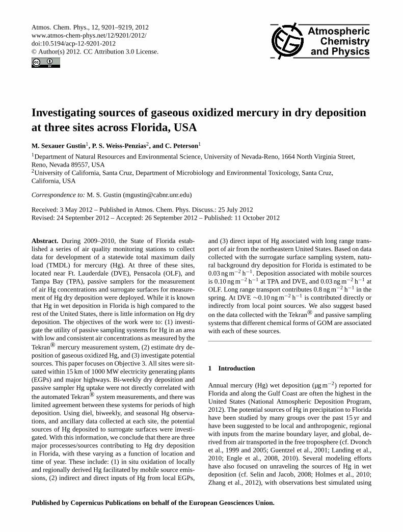
Passive samplers and surrogate surfaces were co-located witha SEARCH, and two Florida Department of Environmen-tal Protection managed locations. A transect was formedby these sampling sites across the State with Davie, nearFort Lauderdale (DVE; Lat. 26.085◦ N, Long. 80.240◦ W)in the southeast; a central location near Tampa (TPA; Lat.27.913◦ N, Long. 82.375◦ W); and a site in the northweston the panhandle at Outlying Landing Field near Pensacola(OLF; Lat. 30.550◦ N, Long. 87.374◦ W). All sites are influ-enced by marine air with the Gulf of Mexico being southof OLF (29 km) and west of TPA (48 km), and the AtlanticOcean 14 km to the east of DVE (Fig. 1). Additional site in-formation is provided in Peterson et al. (2012).

Automated GEM, GOM and PBM data were collected bythe Tekran® system at 5 to 6 m above ground level (a.g.l.)(detection limits 0.1 ng m−3, 1 pg m−3, and 1 pg m−3 respec-tively; Eric Edgerton, personal communication). It is impor-tant to note that variability between co-located instruments

Atmos. Chem. Phys., 12, 9201–9219, 2012 www.atmos-chem-phys.net/12/9201/2012/

http://www.dep.state.fl.us/water/tmdl/merctmdl.htm

http://www.dep.state.fl.us/water/tmdl/merctmdl.htm

M. Sexauer Gustin et al.: Investigating sources of gaseous oxidized mercury in dry deposition 9203

Table 1. General location and emission inventory data for EGPs within a 50 km radius of each site. The 2002 Hg data is from the EPANEI inventory and the 2009 Hg data is from an estimate provided from the Florida Department of Environmental Protection using US EPACAMD hourly heat input data and EPRI correlation coefficients for percent removal.

Facility Nearest Distance to Direction: Site Primary Output Hg Total Hg GOM PBM SO2 NOx COName Site Site (km) to Facility Fuel MW Inventory kg yr−1 kg yr−1 kg yr−1 Mg yr−1 Mg yr−1 Mg yr−1

Year

Wheelabrator North DVE 24 NE Waste 67 2002 46 26 9 163 1250 88Wheelabrator South DVE 5 E Waste 66 2002 53 31 11 131 1214 63Lauderdale DVE 5 E Natural gas 1812 2002 nr nr nr 97 2125 216Port Everglades DVE 13 E Oil 1717 2002 13 4 3 3574 2902 492Covanta (Montanay) DVE 21 SSW Waste 77 2002 7 4 1 27 1150 694Bayside TPA 5 W Natural Gas 1859 2002 3 1 1 17 548 288Big Bend TPA 14 SSW Coal 1995 2009 48 15 1 8725 4387 8317Pasco Co. RRF TPA 33 W Waste 31 2002 14 8 3 14 749 21Bartow TPA 26 W Oil 465 2002 7 2 1 31 456 138Bayboro TPA 35 WSW Oil 232 2002 23 7 5 9 63 0Crist OLF 15 E Coal 1071 2009 70 60 2 3425 5320 545

has been reported to be on the order of 0.3 to 20 % for GEM,9 to 40 % for GOM, and up to 70 % for PBM (Gustin andJaffe, 2010; Steffen et al., 2012). Criteria air pollutants (O3,CO, SO2, NOy and NO) and meteorological parameters weremeasured at 10 m a.g.l. (c.f. Peterson et al., 2012). For alldata, hourly means were time stamped by the end of the hour.For GOM and PBM, this represents the previous two hoursof sampling due to a one hour sampling and analyses cycle.

Surrogate surfaces for GOM dry deposition (ng m−2 h−1)and passive samplers, an indirect measure of GOM (pg h−1)concentrations, were placed at 3 to 5 m a.g.l. (Peterson et al.,2012). These were shipped and deployed over 13 months(n = 28 biweekly samples), from July 2009 through July2010, by State of Florida and SEARCH personnel. Surrogatesurfaces were deployed in triplicate over two weeks with twofield blanks per site. Passive samplers consisted of triplicatemembranes and one membrane blank deployed simultaneousfor each 2 week period. Samplers and membranes were de-ployed, collected and analyzed using a protocol developed byLyman et al. (2009a; 2010). Details regarding quality controlfor this study are reported by Peterson et al. (2012). The sur-rogate surface methods have also been applied by Castro etal. (2012) and recently, in a 2 yr study in the SouthwesternUnited States at 6 locations (Mark Sather, US EPA Region 6,personnel communication, 27 April 2012).

Seasonal mean air Hg, trace gas and meteorological datawere averaged using hourly reported values. Data was bulkedseasonally, where Spring represents March to May, Sum-mer (June–August), Fall (September–November) and Win-ter (December–February). Statistical analyses were done us-ing Minitab®15 and Origin® with a significance level ofp < 0.05 applied.

2.2 Regional emissions inventories

Sources of criteria air pollutants at all three sites are mobileand stationary. In order to support a population of 19×106,the State of Florida has∼90 electrical generation plants

(EGPs) with an output greater than 25 MW (11 coal fired).The impact of these on data collected at each site will de-pend upon wind direction, energy production, fuel type andgeneral proximity. Each site is within 15 km of an EGP pro-ducing greater than 1000 MW and with significantly greaterSO2 emissions relative to other facilities in the vicinity (Ta-ble 1; Fig. 1).

The population of the area will influence the density ofmobile sources. The DVE site, situated in the South FloridaMetropolitan area, hosts 5.6×106 people, and was in closeproximity to US Interstate 595, the Florida Turnpike and thePort Everglades Expressway. The TPA location (populationbase of 4×106) was centered between major routes in andout of the city (i.e. US Interstate 75 and 4). The OLF site islocated to the northwest of Pensacola (population 0.45×106)and just south of US Interstate 10, a major route across north-ern Florida (Fig. 1). The population of Florida increases sea-sonally during the winter and spring when tourism is a majorindustry. In 2008, there were an estimated 82.5×106 visitorsto the State (http://www.floridatransportationindicators.org).

For our data analyses annual SO2 and NOx emis-sions inventories for EGPs in Florida were obtainedfrom the Florida Department of Environmental Pro-tection website (http://webapps.dep.state.fl.us/DarmReports/eaor/fads/search.do), and daily values from the US EPAClean Air Markets Division website (http://ampd.epa.gov/ampd/) (Table 1). NOx/SO2 ratios for each facility were de-termined from reported output in tons by converting to molesusing the molar mass for SO2 and NO2, and then calculatingthe ratio NOx/SO2.

Mercury emissions for EGPs that were not coal fired wereestimated using data from the 2002 EPA NEI (http://ampd.epa.gov/ampd/). For the coal burning utilities, emission datafor 2009 were obtained from the Florida Division of Envi-ronmental Protection (Greg White, Florida Division of Envi-ronmental Quality, personal communication, August 2011).The latter were from the Florida Electric Power Coordina-tion Group, Inc. and based on the US EPA Clean Air Markets

www.atmos-chem-phys.net/12/9201/2012/ Atmos. Chem. Phys., 12, 9201–9219, 2012

http://www.floridatransportationindicators.org

http://webapps.dep.state.fl.us/DarmReports/eaor/fads/search.do

http://webapps.dep.state.fl.us/DarmReports/eaor/fads/search.do

http://ampd.epa.gov/ampd/





Figure 1: A) Map of Florida, located in the southeastern United States, showing the study locations and Florida electrical generation units (EGPs) with > 1000 MW output segregated by primary fuel type. Also shown are more detailed maps of area surrounding study sites and all EGUs within a 50 km radius for B) Pensacola, C) Tampa and D) Ft. Lauderdale areas.

A B

C D

Fig. 1. (A) Map of Florida, located in the southeastern United States, showing the study locations and Florida electrical generation units(EGUs) with> 1000 MW output segregated by primary fuel type. Also shown are more detailed maps of area surrounding study sites and allEGPs within a 50 km radius for(B) Pensacola,(C) Tampa and(D) Ft. Lauderdale areas.

Division (CAMD) hourly heat input data and Electric PowerResearch Institute (EPRI) correlation coefficients for percentremoval for 2009. Based on these, total Hg and GOM emis-sions for Plant Crist were by far the largest for any singlefacility. However, a flue gas desulfurization (FGD) systemcame online at the site in December 2009 and as such; theinventory values do not reflect those for the entire study. Itis important to note for the incinerators and oil based facil-ities, it is unclear whether emission estimates are based onempirical data (Table 1).

2.3 Classification of GOM data

Following the approach outlined in Weiss-Penzias etal. (2011), GOM concentration enhancement “events” are de-fined as time periods when at least one GOM concentrationmeasurement from the Tekran® system was greater than the97th percentile based on all concentrations at each site (31,11, and 16 pg m−3 for DVE, OLF and TPA, respectively).The duration of the event was then designated as the timeover which the Tekran® derived GOM concentrations wereat or above the annual mean for each site (Supplement Ta-bles 1 and 2). Events were then classified as “1”, “2”, or



“Unclassified” based on SO2 concentrations and wind direc-tions during the peak GOM concentrations. Class 1 eventsinclude those when SO2 concentrations were greater than themean of peak SO2 values for all events at each site, and whenconcurrent wind directions were from the closest large EGP:70 to 110 degrees for both DVE and OLF, and 160–200 de-grees for TPA. Conversely, Class 2 events had peak SO2 con-centrations that were less than the mean of all events andwind directions from outside the ranges stated for Class 1events. Unclassified events met the GOM criteria but not theSO2 and wind direction criteria for the Class 1 or Class 2events.

2.4 Back trajectory analysis

Seventy-two hour back trajectories were calculated usingHYSPLIT v4.8 (Draxler and Hess, 1997) for the 5 eventswith the highest GOM concentrations. Meteorological fieldsat 40 km resolution from the National Center for Environ-mental Prediction Eta Data Assimilation System (EDAS)served as input for the procedure. Trajectories were initial-ized at 6 h intervals during the 24-h period encompassingthe peak GOM concentration of each event. The area of ini-tialization was a 0.5× 0.5 degree grid of 9 starting locationsevenly spaced around each site. Four starting altitudes wereused: 500, 1000, 1500, and 2000 m above modeled groundlevel. The goal of using trajectory analysis in this study wasto investigate regional and larger scale transport patterns thatmay have influenced GOM and GOM dry deposition. Assuch, it is common practice to have the lowest starting alti-tude be well above the surface, to avoid erroneous trajectoriesdue to sub-grid processes and turbulent flow. This generated144 back trajectories for each event. Each hourly location ofa trajectory is denoted as a “trajectory point”.

Gridded frequency distributions (GFDs) were generatedby averaging the number of trajectory points in 1× 1 de-gree grid cells over the domain of interest (Weiss-Penziaset al., 2009, 2011). GFDs were also generated to show onlythose grid cells that contained a high proportion (>90 %) ofthe trajectory points that were at altitudes greater than theHYSPLIT modeled boundary layer height, and the distribu-tion of precipitation along the trajectory paths. The locationprobability represents the fraction of trajectory points in agiven cell relative to the number of trajectory points in themost populated cell. Uncertainties in the three-dimensionallocations of trajectories (the horizontal uncertainty is roughly20 % of the distance traveled) were minimized by calculat-ing trajectories at the nine locations and four altitudes aroundeach sampling site, thus creating a data set with sufficient sta-tistical power to overcome the major limitations of the com-putational procedure (sub grid processes, turbulent flow, andconvection; Stohl, 1998; Stohl et al., 2003).

2.5 Meso- and synoptic scale wind patterns in Florida

When interpreting trends in air pollutants, one must considerthe meso- and synoptic- scale meteorological conditions im-pacting each site. On the synoptic scale during the coolerseasons, the near surface flow in Florida is dominated bypassing cold fronts. This is especially true for North Floridasince not all fronts reach South Florida. The winds typicallyare from the west or northwest after frontal passage and thenshifts to the south after several days with the approach of thenext frontal systems. In the middle and upper levels of theatmosphere, the cooler season flow is dominated by passingtroughs and ridges. The flow generally is from the southwestahead of a trough and from the northwest after the troughpasses (before the next ridge arrives). Once again, this is mostpronounced for North Florida.

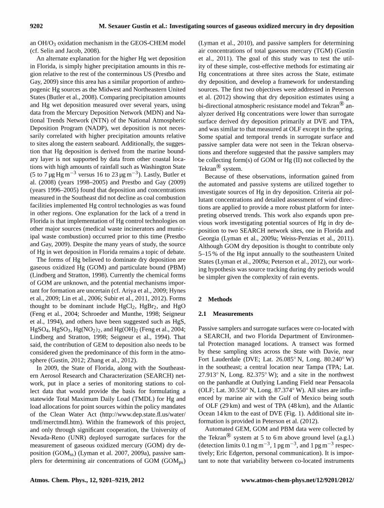
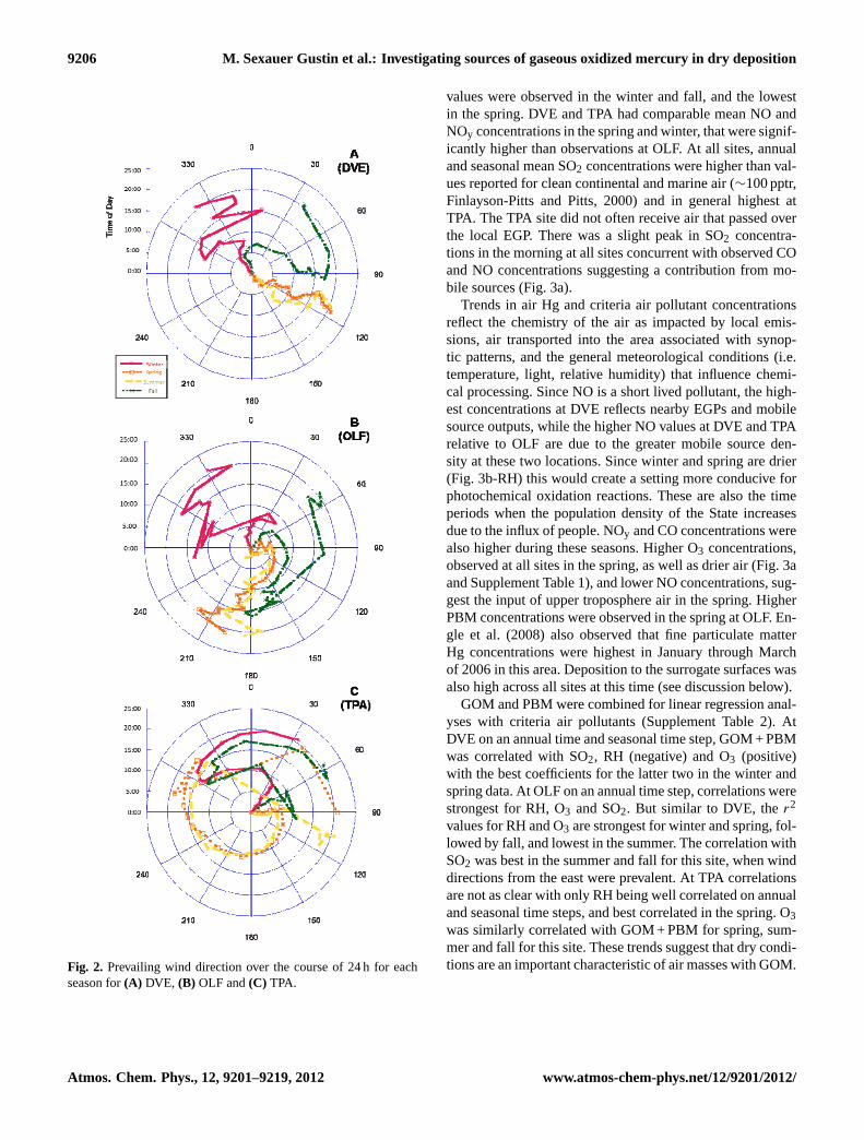
During the summer, synoptic patterns in Florida are dom-inated by the Bermuda/Azores high, and a lobe of high pres-sure that sometimes forms over the Gulf of Mexico. Depend-ing on the location of the Bermuda high and whether thereis a Gulf of Mexico lobe, both the surface and upper levelwinds can range from east, to south, to west, and occasion-ally, have a component from the north. Summer is the seabreeze season in Florida, and the three sampling sites expe-rience a regular diel variation of this meso-scale circulation,i.e. onshore flow during the day (sea breeze) and weaker off-shore flow at night (land breeze) (Fig. 2). The direction andstrength of the large scale flow greatly affects the intensityand strength and inland penetration of the sea breeze (HenryFuelberg, Florida State University, personal communication,31 March and 2 May 2012).

3 Results

3.1 Summary of observations and interspeciescorrelations

As summarized by Peterson et al. (2012), annual GOM con-centrations as measured by the Tekran® system at DVE(7 pg m−3) were significantly (p < 0.05) higher than thosemeasured at OLF (2 pg m−3) and TPA (3 pg m−3) (Supple-ment Table 1). Annual GEM concentrations were also signif-icantly higher at DVE (1.4 versus 1.2 and 1.3 ng m−3, respec-tively). PBM concentrations were significantly higher at OLFrelative to the two other sites (3 versus 2 pg m−3 p < 0.05).

Mean annual and seasonal ozone (O3) concentrations werehighest at OLF, with those measured at DVE and TPA beingsimilar to each other. Highest O3 values were observed at allsites in the spring. Mean seasonal and annual CO concentra-tions were highest in the winter and lowest in the summer atall sites, and highest at TPA relative to the other sites. Sea-sonal mean CO values are at or above the upper limit of thoseconsidered ambient values for remote areas of 50 to 150 ppb(Finlayson-Pitts and Pitts, 2000). The highest NO and NOy



Figure 2: Prevailing wind direction over the course of 24 hours for each season for A) DVE, B) OLF and C) TPA.

Fig. 2. Prevailing wind direction over the course of 24 h for eachseason for(A) DVE, (B) OLF and(C) TPA.

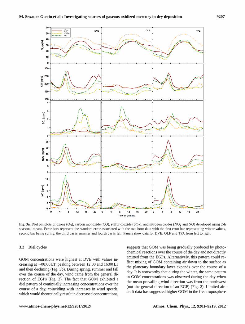
values were observed in the winter and fall, and the lowestin the spring. DVE and TPA had comparable mean NO andNOy concentrations in the spring and winter, that were signif-icantly higher than observations at OLF. At all sites, annualand seasonal mean SO2 concentrations were higher than val-ues reported for clean continental and marine air (∼100 pptr,Finlayson-Pitts and Pitts, 2000) and in general highest atTPA. The TPA site did not often receive air that passed overthe local EGP. There was a slight peak in SO2 concentra-tions in the morning at all sites concurrent with observed COand NO concentrations suggesting a contribution from mo-bile sources (Fig. 3a).

Trends in air Hg and criteria air pollutant concentrationsreflect the chemistry of the air as impacted by local emis-sions, air transported into the area associated with synop-tic patterns, and the general meteorological conditions (i.e.temperature, light, relative humidity) that influence chemi-cal processing. Since NO is a short lived pollutant, the high-est concentrations at DVE reflects nearby EGPs and mobilesource outputs, while the higher NO values at DVE and TPArelative to OLF are due to the greater mobile source den-sity at these two locations. Since winter and spring are drier(Fig. 3b-RH) this would create a setting more conducive forphotochemical oxidation reactions. These are also the timeperiods when the population density of the State increasesdue to the influx of people. NOy and CO concentrations werealso higher during these seasons. Higher O3 concentrations,observed at all sites in the spring, as well as drier air (Fig. 3aand Supplement Table 1), and lower NO concentrations, sug-gest the input of upper troposphere air in the spring. HigherPBM concentrations were observed in the spring at OLF. En-gle et al. (2008) also observed that fine particulate matterHg concentrations were highest in January through Marchof 2006 in this area. Deposition to the surrogate surfaces wasalso high across all sites at this time (see discussion below).

GOM and PBM were combined for linear regression anal-yses with criteria air pollutants (Supplement Table 2). AtDVE on an annual time and seasonal time step, GOM + PBMwas correlated with SO2, RH (negative) and O3 (positive)with the best coefficients for the latter two in the winter andspring data. At OLF on an annual time step, correlations werestrongest for RH, O3 and SO2. But similar to DVE, ther2

values for RH and O3 are strongest for winter and spring, fol-lowed by fall, and lowest in the summer. The correlation withSO2 was best in the summer and fall for this site, when winddirections from the east were prevalent. At TPA correlationsare not as clear with only RH being well correlated on annualand seasonal time steps, and best correlated in the spring. O3was similarly correlated with GOM + PBM for spring, sum-mer and fall for this site. These trends suggest that dry condi-tions are an important characteristic of air masses with GOM.


M. Sexauer Gustin et al.: Investigating sources of gaseous oxidized mercury in dry deposition 9207Figure 3A:

Fig. 3a.Diel bin plots of ozone (O3), carbon monoxide (CO), sulfur dioxide (SO2), and nitrogen oxides (NOy and NO) developed using 2-hseasonal means. Error bars represent the standard error associated with the two hour data with the first error bar representing winter values,second bar being spring, the third bar is summer and fourth bar is fall. Panels show data for DVE, OLF and TPA from left to right.

3.2 Diel cycles

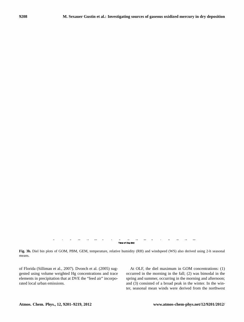
GOM concentrations were highest at DVE with values in-creasing at∼08:00 LT, peaking between 12:00 and 16:00 LTand then declining (Fig. 3b). During spring, summer and fallover the course of the day, wind came from the general di-rection of EGPs (Fig. 2). The fact that GOM exhibited adiel pattern of continually increasing concentrations over thecourse of a day, coinciding with increases in wind speeds,which would theoretically result in decreased concentrations,

suggests that GOM was being gradually produced by photo-chemical reactions over the course of the day and not directlyemitted from the EGPs. Alternatively, this pattern could re-flect mixing of GOM containing air down to the surface asthe planetary boundary layer expands over the course of aday. It is noteworthy that during the winter, the same patternin GOM concentrations was observed during the day whenthe mean prevailing wind direction was from the northwest(not the general direction of an EGP) (Fig. 2). Limited air-craft data has suggested higher GOM in the free troposphere


9208 M. Sexauer Gustin et al.: Investigating sources of gaseous oxidized mercury in dry depositionFigure 3B:

Fig. 3b. Diel bin plots of GOM, PBM, GEM, temperature, relative humidity (RH) and windspeed (WS) also derived using 2-h seasonalmeans.

of Florida (Silliman et al., 2007). Dvonch et al. (2005) sug-gested using volume weighted Hg concentrations and traceelements in precipitation that at DVE the “feed air” incorpo-rated local urban emissions.

At OLF, the diel maximum in GOM concentrations: (1)occurred in the morning in the fall; (2) was bimodal in thespring and summer, occurring in the morning and afternoon;and (3) consisted of a broad peak in the winter. In the win-ter, seasonal mean winds were derived from the northwest



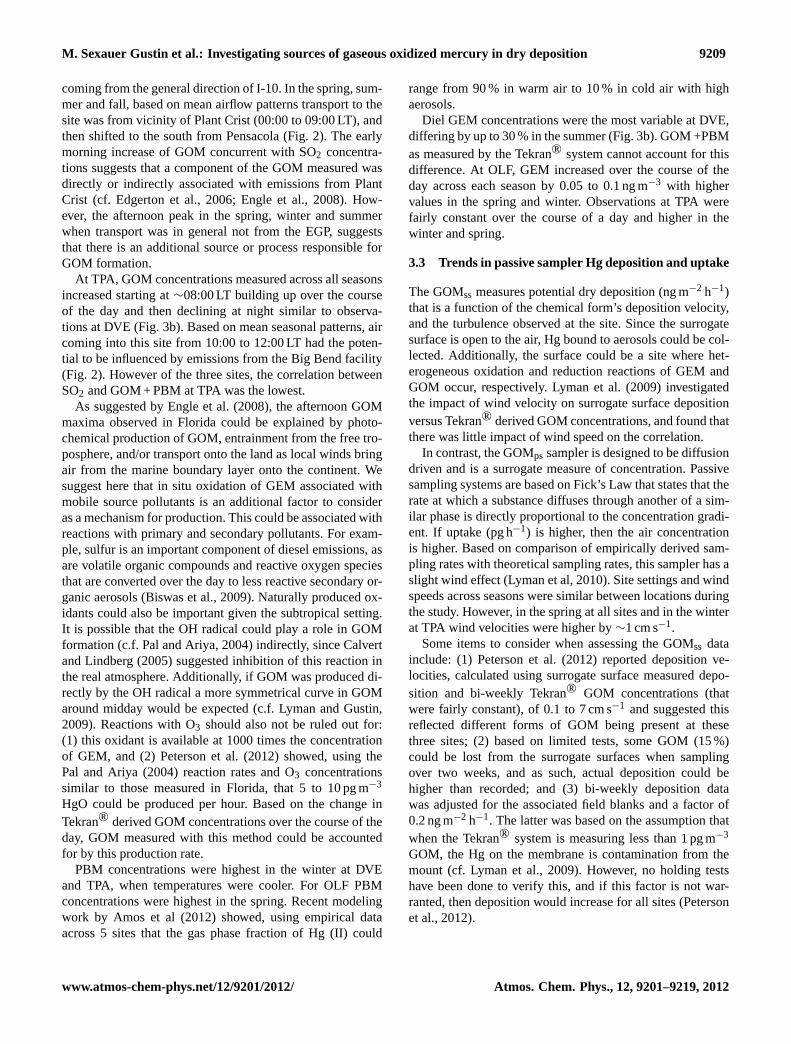
coming from the general direction of I-10. In the spring, sum-mer and fall, based on mean airflow patterns transport to thesite was from vicinity of Plant Crist (00:00 to 09:00 LT), andthen shifted to the south from Pensacola (Fig. 2). The earlymorning increase of GOM concurrent with SO2 concentra-tions suggests that a component of the GOM measured wasdirectly or indirectly associated with emissions from PlantCrist (cf. Edgerton et al., 2006; Engle et al., 2008). How-ever, the afternoon peak in the spring, winter and summerwhen transport was in general not from the EGP, suggeststhat there is an additional source or process responsible forGOM formation.

At TPA, GOM concentrations measured across all seasonsincreased starting at∼08:00 LT building up over the courseof the day and then declining at night similar to observa-tions at DVE (Fig. 3b). Based on mean seasonal patterns, aircoming into this site from 10:00 to 12:00 LT had the poten-tial to be influenced by emissions from the Big Bend facility(Fig. 2). However of the three sites, the correlation betweenSO2 and GOM + PBM at TPA was the lowest.

As suggested by Engle et al. (2008), the afternoon GOMmaxima observed in Florida could be explained by photo-chemical production of GOM, entrainment from the free tro-posphere, and/or transport onto the land as local winds bringair from the marine boundary layer onto the continent. Wesuggest here that in situ oxidation of GEM associated withmobile source pollutants is an additional factor to consideras a mechanism for production. This could be associated withreactions with primary and secondary pollutants. For exam-ple, sulfur is an important component of diesel emissions, asare volatile organic compounds and reactive oxygen speciesthat are converted over the day to less reactive secondary or-ganic aerosols (Biswas et al., 2009). Naturally produced ox-idants could also be important given the subtropical setting.It is possible that the OH radical could play a role in GOMformation (c.f. Pal and Ariya, 2004) indirectly, since Calvertand Lindberg (2005) suggested inhibition of this reaction inthe real atmosphere. Additionally, if GOM was produced di-rectly by the OH radical a more symmetrical curve in GOMaround midday would be expected (c.f. Lyman and Gustin,2009). Reactions with O3 should also not be ruled out for:(1) this oxidant is available at 1000 times the concentrationof GEM, and (2) Peterson et al. (2012) showed, using thePal and Ariya (2004) reaction rates and O3 concentrationssimilar to those measured in Florida, that 5 to 10 pg m−3

HgO could be produced per hour. Based on the change inTekran® derived GOM concentrations over the course of theday, GOM measured with this method could be accountedfor by this production rate.

PBM concentrations were highest in the winter at DVEand TPA, when temperatures were cooler. For OLF PBMconcentrations were highest in the spring. Recent modelingwork by Amos et al (2012) showed, using empirical dataacross 5 sites that the gas phase fraction of Hg (II) could

range from 90 % in warm air to 10 % in cold air with highaerosols.

Diel GEM concentrations were the most variable at DVE,differing by up to 30 % in the summer (Fig. 3b). GOM +PBMas measured by the Tekran® system cannot account for thisdifference. At OLF, GEM increased over the course of theday across each season by 0.05 to 0.1 ng m−3 with highervalues in the spring and winter. Observations at TPA werefairly constant over the course of a day and higher in thewinter and spring.

3.3 Trends in passive sampler Hg deposition and uptake

The GOMss measures potential dry deposition (ng m−2 h−1)that is a function of the chemical form’s deposition velocity,and the turbulence observed at the site. Since the surrogatesurface is open to the air, Hg bound to aerosols could be col-lected. Additionally, the surface could be a site where het-erogeneous oxidation and reduction reactions of GEM andGOM occur, respectively. Lyman et al. (2009) investigatedthe impact of wind velocity on surrogate surface depositionversus Tekran® derived GOM concentrations, and found thatthere was little impact of wind speed on the correlation.

In contrast, the GOMps sampler is designed to be diffusiondriven and is a surrogate measure of concentration. Passivesampling systems are based on Fick’s Law that states that therate at which a substance diffuses through another of a sim-ilar phase is directly proportional to the concentration gradi-ent. If uptake (pg h−1) is higher, then the air concentrationis higher. Based on comparison of empirically derived sam-pling rates with theoretical sampling rates, this sampler has aslight wind effect (Lyman et al, 2010). Site settings and windspeeds across seasons were similar between locations duringthe study. However, in the spring at all sites and in the winterat TPA wind velocities were higher by∼1 cm s−1.

Some items to consider when assessing the GOMss datainclude: (1) Peterson et al. (2012) reported deposition ve-locities, calculated using surrogate surface measured depo-sition and bi-weekly Tekran® GOM concentrations (thatwere fairly constant), of 0.1 to 7 cm s−1 and suggested thisreflected different forms of GOM being present at thesethree sites; (2) based on limited tests, some GOM (15 %)could be lost from the surrogate surfaces when samplingover two weeks, and as such, actual deposition could behigher than recorded; and (3) bi-weekly deposition datawas adjusted for the associated field blanks and a factor of0.2 ng m−2 h−1. The latter was based on the assumption thatwhen the Tekran® system is measuring less than 1 pg m−3

GOM, the Hg on the membrane is contamination from themount (cf. Lyman et al., 2009). However, no holding testshave been done to verify this, and if this factor is not war-ranted, then deposition would increase for all sites (Petersonet al., 2012).



Figure 4: Seasonal means ± 1 sd of Tekran-GOM air concentration (GOMT), GOM dry deposition to a surrogate surface (GOMSS), and GOM uptake to a passive sampler (GOMPS) measured at DVE, OLF and TPA.

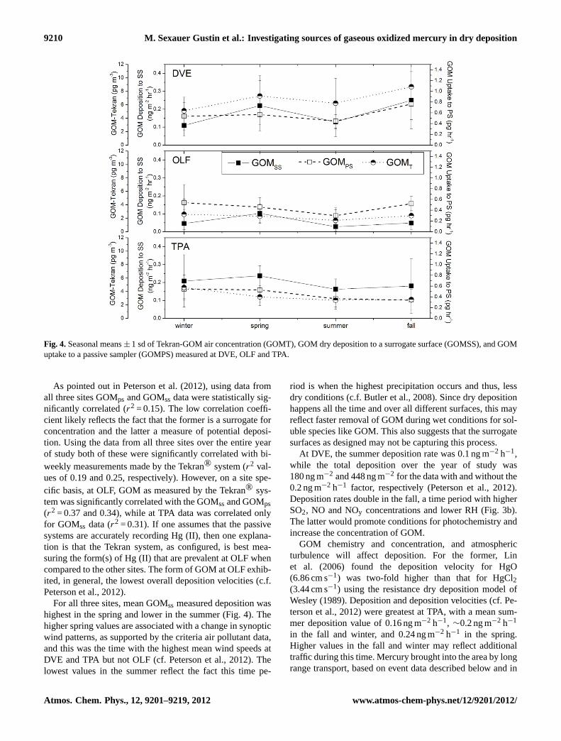
Fig. 4.Seasonal means± 1 sd of Tekran-GOM air concentration (GOMT), GOM dry deposition to a surrogate surface (GOMSS), and GOMuptake to a passive sampler (GOMPS) measured at DVE, OLF and TPA.

As pointed out in Peterson et al. (2012), using data fromall three sites GOMps and GOMss data were statistically sig-nificantly correlated (r2 = 0.15). The low correlation coeffi-cient likely reflects the fact that the former is a surrogate forconcentration and the latter a measure of potential deposi-tion. Using the data from all three sites over the entire yearof study both of these were significantly correlated with bi-weekly measurements made by the Tekran® system (r2 val-ues of 0.19 and 0.25, respectively). However, on a site spe-cific basis, at OLF, GOM as measured by the Tekran® sys-tem was significantly correlated with the GOMssand GOMps(r2 = 0.37 and 0.34), while at TPA data was correlated onlyfor GOMss data (r2 = 0.31). If one assumes that the passivesystems are accurately recording Hg (II), then one explana-tion is that the Tekran system, as configured, is best mea-suring the form(s) of Hg (II) that are prevalent at OLF whencompared to the other sites. The form of GOM at OLF exhib-ited, in general, the lowest overall deposition velocities (c.f.Peterson et al., 2012).

For all three sites, mean GOMss measured deposition washighest in the spring and lower in the summer (Fig. 4). Thehigher spring values are associated with a change in synopticwind patterns, as supported by the criteria air pollutant data,and this was the time with the highest mean wind speeds atDVE and TPA but not OLF (cf. Peterson et al., 2012). Thelowest values in the summer reflect the fact this time pe-

riod is when the highest precipitation occurs and thus, lessdry conditions (c.f. Butler et al., 2008). Since dry depositionhappens all the time and over all different surfaces, this mayreflect faster removal of GOM during wet conditions for sol-uble species like GOM. This also suggests that the surrogatesurfaces as designed may not be capturing this process.

At DVE, the summer deposition rate was 0.1 ng m−2 h−1,while the total deposition over the year of study was180 ng m−2 and 448 ng m−2 for the data with and without the0.2 ng m−2 h−1 factor, respectively (Peterson et al., 2012).Deposition rates double in the fall, a time period with higherSO2, NO and NOy concentrations and lower RH (Fig. 3b).The latter would promote conditions for photochemistry andincrease the concentration of GOM.

GOM chemistry and concentration, and atmosphericturbulence will affect deposition. For the former, Linet al. (2006) found the deposition velocity for HgO(6.86 cm s−1) was two-fold higher than that for HgCl2(3.44 cm s−1) using the resistance dry deposition model ofWesley (1989). Deposition and deposition velocities (cf. Pe-terson et al., 2012) were greatest at TPA, with a mean sum-mer deposition value of 0.16 ng m−2 h−1, ∼0.2 ng m−2 h−1

in the fall and winter, and 0.24 ng m−2 h−1 in the spring.Higher values in the fall and winter may reflect additionaltraffic during this time. Mercury brought into the area by longrange transport, based on event data described below and in



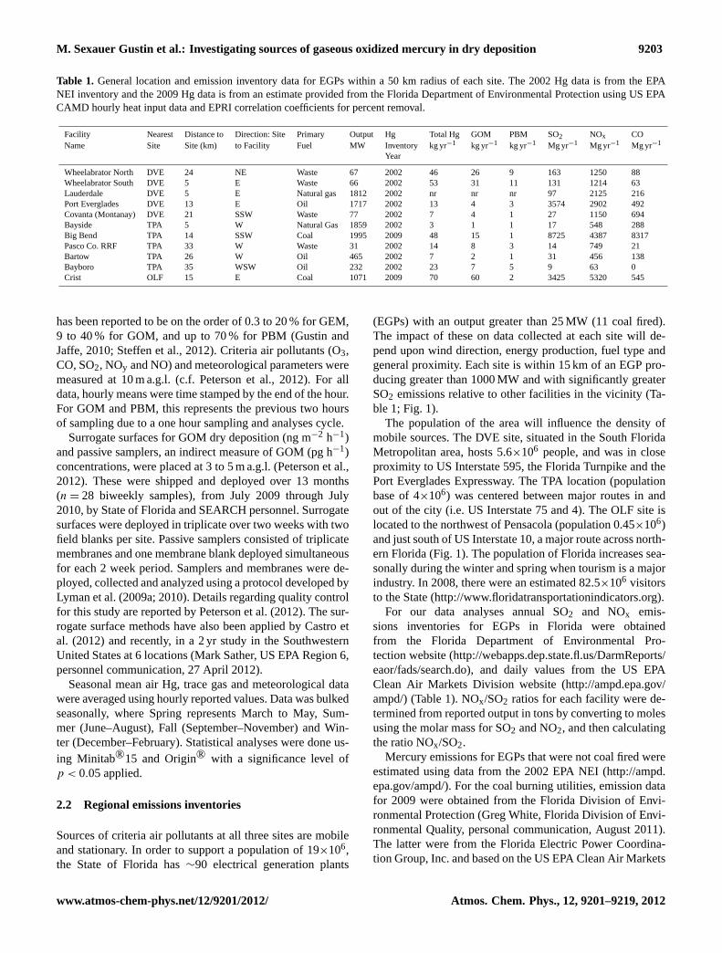
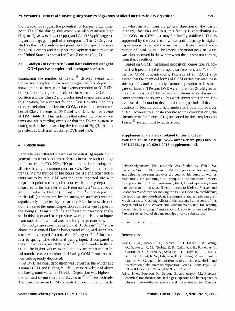
Figure 5: Gridded frequency distributions of back trajectories for the five highest GOM concentration event days Classes 1 and 2 at the DVE site. A) Horizontal location probabilities for Class 1 events. B) Horizontal location probabilities for Class 2 events. C) Same as A, but with color removed from grid cells with > 90% of trajectory points having altitudes below the modeled boundary layer. D) Same as C except for Class 2 events. E) and F) Modeled precipitation distributions for Classes 1 and 2 events overlain on the horizontal location probabilities.

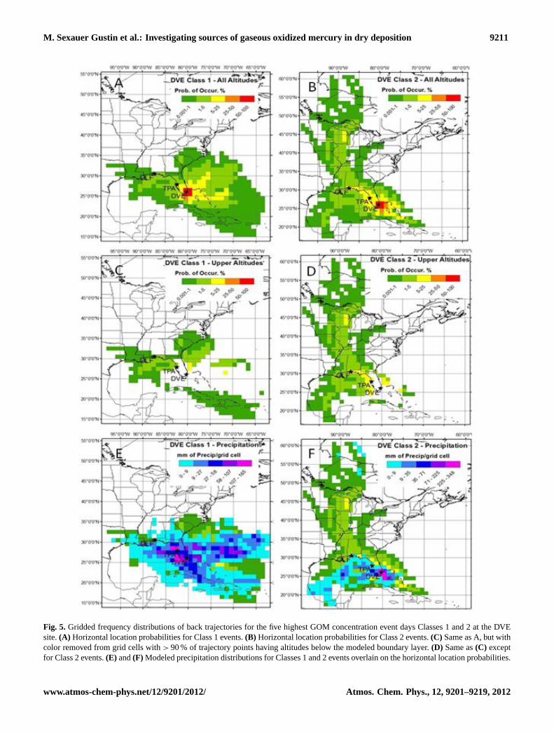
Fig. 5. Gridded frequency distributions of back trajectories for the five highest GOM concentration event days Classes 1 and 2 at the DVEsite.(A) Horizontal location probabilities for Class 1 events.(B) Horizontal location probabilities for Class 2 events.(C) Same as A, but withcolor removed from grid cells with> 90 % of trajectory points having altitudes below the modeled boundary layer.(D) Same as(C) exceptfor Class 2 events.(E) and(F) Modeled precipitation distributions for Classes 1 and 2 events overlain on the horizontal location probabilities.



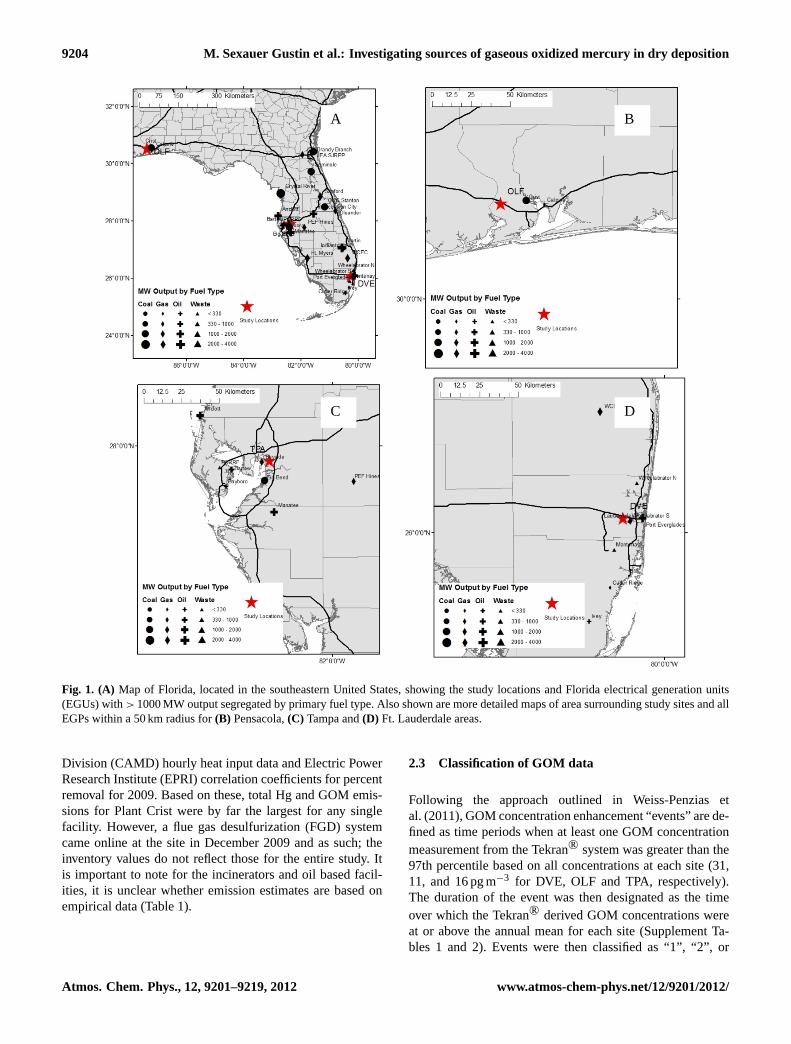
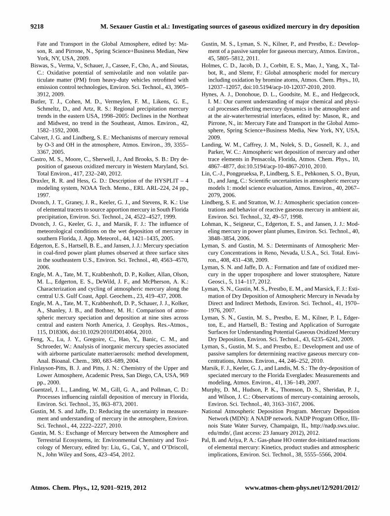
Figure 6: Gridded frequency distributions of back trajectories for the five highest GOM concentration event days Classes 1 and 2 at the OLF site. A) Horizontal location probabilities for Class 1 events. B) Horizontal location probabilities for Class 2 events. C) Same as A, but with color removed from grid cells with > 90% of trajectory points having altitudes below the modeled boundary layer. D) Same as C except for Class 2 events. E) and F) Modeled precipitation distributions for Classes 1 and 2 events overlain on the horizontal location probabilities.

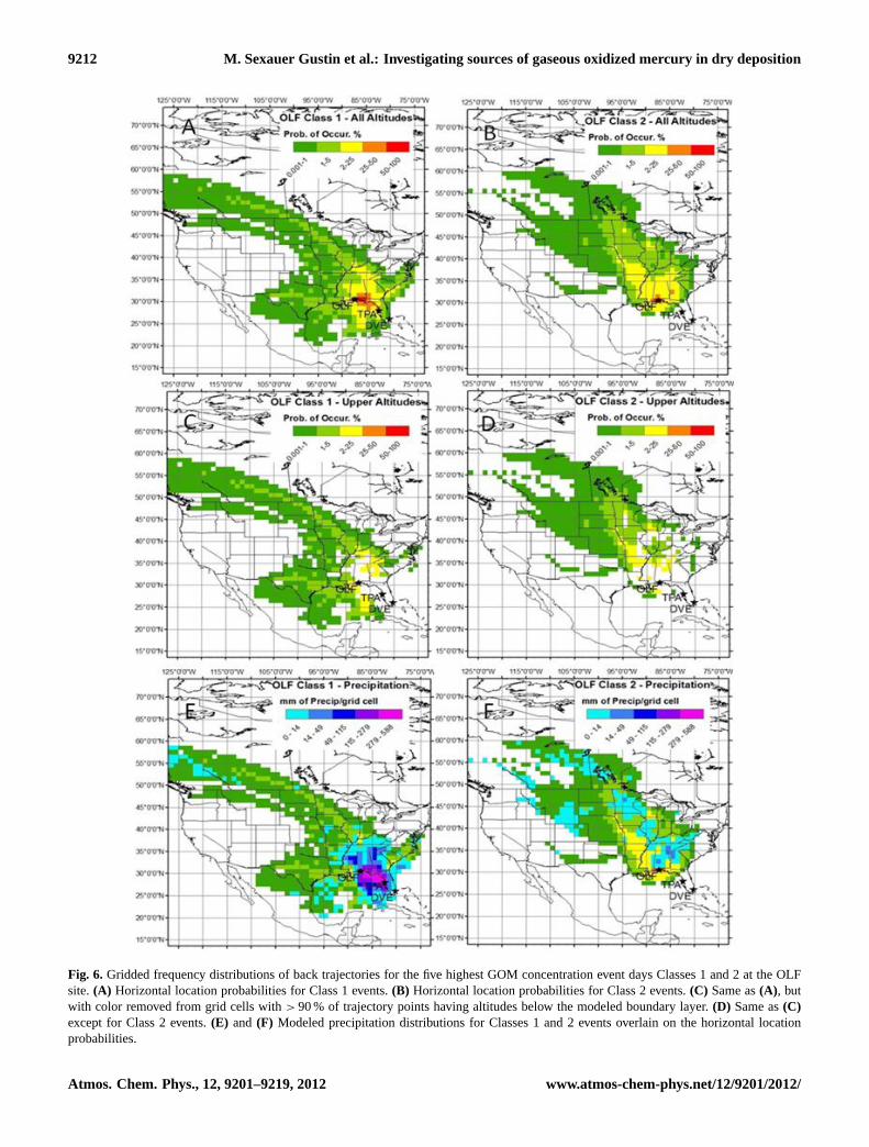
Fig. 6. Gridded frequency distributions of back trajectories for the five highest GOM concentration event days Classes 1 and 2 at the OLFsite.(A) Horizontal location probabilities for Class 1 events.(B) Horizontal location probabilities for Class 2 events.(C) Same as(A), butwith color removed from grid cells with> 90 % of trajectory points having altitudes below the modeled boundary layer.(D) Same as(C)except for Class 2 events.(E) and (F) Modeled precipitation distributions for Classes 1 and 2 events overlain on the horizontal locationprobabilities.



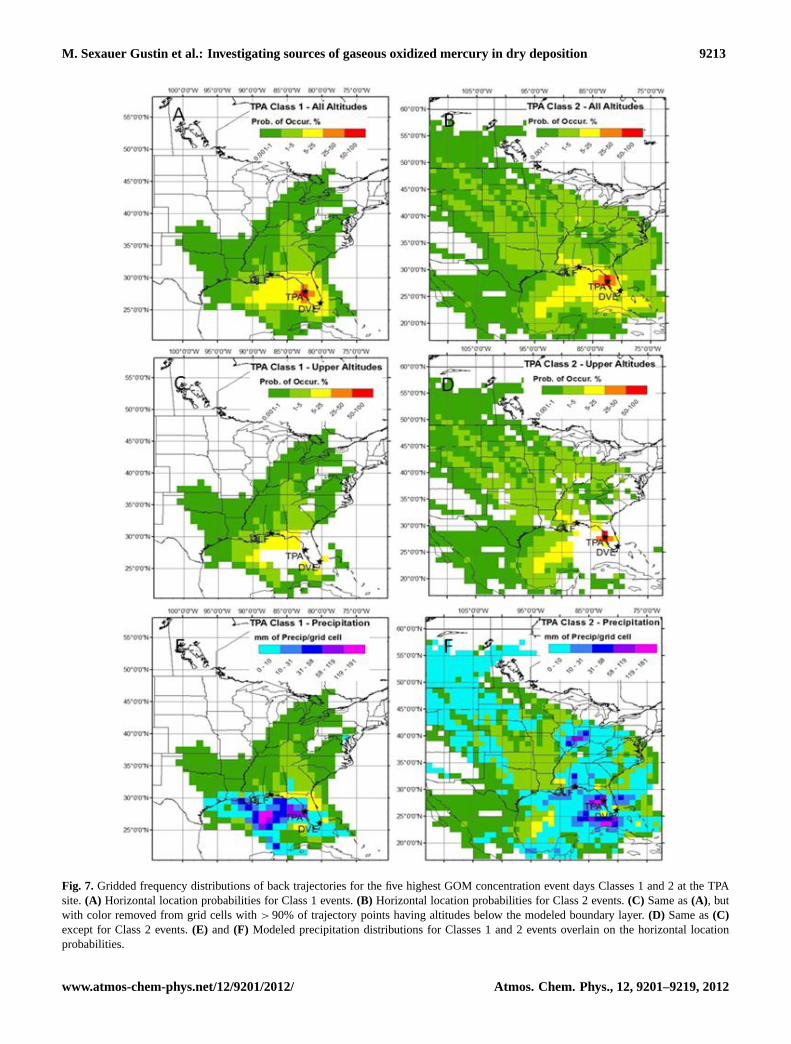
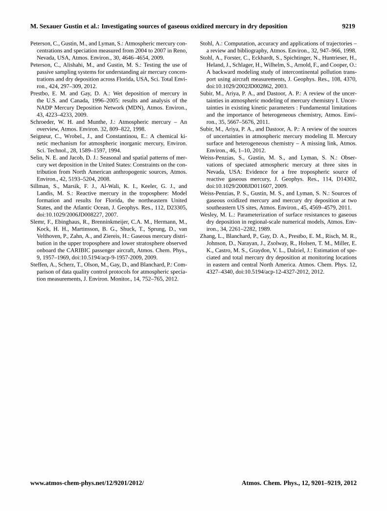
Figure 7: Gridded frequency distributions of back trajectories for the five highest GOM concentration event days Classes 1 and 2 at the TPA site. A) Horizontal location probabilities for Class 1 events. B) Horizontal location probabilities for Class 2 events. C) Same as A, but with color removed from grid cells with > 90% of trajectory points having altitudes below the modeled boundary layer. D) Same as C except for Class 2 events. E) and F) Modeled precipitation distributions for Classes 1 and 2 events overlain on the horizontal location probabilities.

Fig. 7. Gridded frequency distributions of back trajectories for the five highest GOM concentration event days Classes 1 and 2 at the TPAsite.(A) Horizontal location probabilities for Class 1 events.(B) Horizontal location probabilities for Class 2 events.(C) Same as(A), butwith color removed from grid cells with> 90% of trajectory points having altitudes below the modeled boundary layer.(D) Same as(C)except for Class 2 events.(E) and (F) Modeled precipitation distributions for Classes 1 and 2 events overlain on the horizontal locationprobabilities.



Weiss Penzias et al. (2011), is likely contributing to the ad-ditional deposition measured in the spring (see below eventanalyses). At OLF, mean deposition was∼2 times higher inthe spring (0.11 ng m−2 h−1) relative to the winter, summerand fall (0.06, 0.03, and 0.03 ng m−2 h−1, respectively). Thehigher summer value at TPA relative to the other sites maybe due to the location of the sampling site in an area of hightraffic density. Since the Tekran® measured GOM air con-centrations were similar between OLF and TPA this suggestsa higher dry deposition velocity for the form occurring at thissite and that it was not being measured by this instrument.

It is noteworthy here, that Marsik et al. (2007), using awater based surrogate surface positioned over a mixed sawgrass and cattail stand in Florida in Feb to March 1999 andJune 2000, obtained dry deposition rates of 0.5 ng m−2 h−1

and 0.24 ng m−2 h−1, respectively, with spring rates be-ing greater. Our values would be more comparable if the0.2 ng m−2 h−1 adjustment factor was not applied. Also, pre-vious work done in 2007–2008 also showed that GOMss de-position was enhanced during the spring relative to other sea-sons at the OLF site and another site near Atlanta (YRK)(Lyman et al., 2009; Weiss-Penzias et al., 2011).

Assuming passive sampler uptake is an indicator of airconcentrations, annual averages showed DVE> TPA> OLFwith lowest mean value reported for the summer at all threesites. The highest period GOMps uptake was the winter atDVE; winter and fall at OLF; and winter and spring at TPA.These are time periods associated with increased mobilesources density at all sites, and long range transport at TPA.

Peterson et al. (2012) showed that 2-week integratedTekran-GOM was weakly correlated with GOMss, andGOMps observations for all sites; but on an individual sitebasis only well correlated at OLF. This is in contrast to pre-vious work (Lyman et al., 2009,2010; Castro et al., 2012)that showed for rural areas, observations made with these twomethods were correlated. Using an inferential model (Zhanget al., 2012) showed that deposition measured with thesesamplers was similar to modeled values measured in a ru-ral area in Maryland, USA. In contrast, Peterson et al. (2012)and Lyman et al. (2007) showed using a similar model thatsurrogate surface deposition was underestimated. Peterson etal. (2012) found the model better simulated deposition mea-sured at OLF relative to TPA and DVE. Lyman et al. (2007)found that the GOMss deposition was consistently higherthan the modeled value and the disparity was not consistentacross all seasons. Model outputs will be impacted by theparameters used and the assumptions applied. The use of thevalues of alpha and beta in the model developed by Lymanet al (2007), applied by Peterson et al (2012), were modifiedbased on based on the expected chemistry of GOM instead ofusing HNO3. Lyman et al. (2007) showed through sensitivityanalyses that changes in chemical species dependent valuesand land use categories could significantly impact model de-position velocities. Based on these observations we hypoth-

esize that use of one chemical species in a model may notallow for adequate simulation of dry deposition across spaceand time.

3.4 Detailed analysis of GOM events

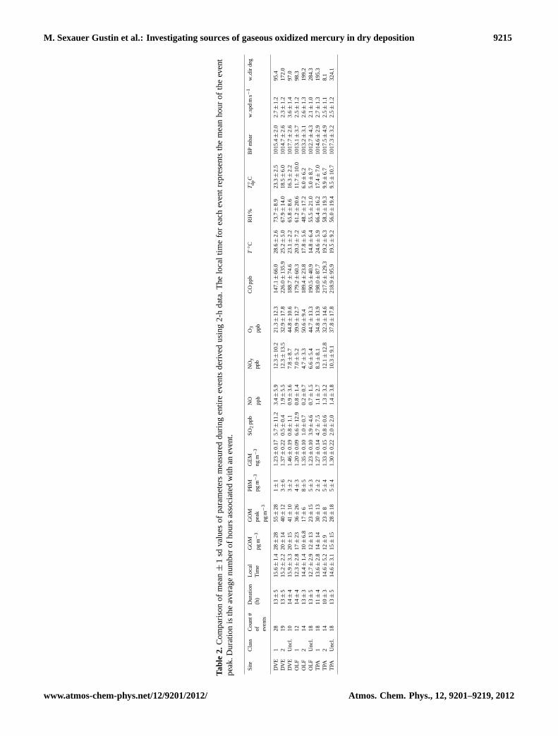
GOM events occurred most often in the late morning and af-ternoon, with none at night. Most events occurred on differ-ent days. With respect to all three types of events, mean GOMconcentrations were highest and GEM lowest in associationwith Class 1 events, while PBM concentrations were highestin Class 2 events (Table 2). Mean dewpoint temperature (Tdp)was higher in the Class 1 events for all sites, while for Class 2and Unclassified events values were comparable. As spec-ified, Class 1 events had wind directions from the generaldirection of the EGPs, while Class 2 events were not fromthis direction and predominantly from the north and south.In general, Unclassified events originated from the north.

Using the mean values in Table 2, for DVE and OLF,Class 1 events had lower O3 and higher NO concentrationsthan Class 2 and Unclassified events, but these were simi-lar across events at TPA. The criteria pollutant concentra-tions during Class 1 events suggest that pollutants from localsource are contributing. Class 1 events tended to occur in thefall at DVE (52 %) and at OLF (50 %), when prevailing winddirections were from the direction of the local EGPs (Fig. 2).The mean peak GOM concentration was∼15 pg m−3 higherfor Class 1 versus Class 2 events at all sites. In contrast, theaverage over the entire event was∼7 pg m−3 higher for DVEand OLF but not TPA. We suggest that during these selectedevents the EGP are indirectly and directly contributing GOMto the sites. CO was higher in Class 2 and Unclassified eventsat DVE and OLF, but the same at TPA across events. At TPA,NOy was lower in Class 1 events while NO was consistentacross events.

Looking in detail at the NOy versus SO2 relationships dur-ing Class 1 events (Supplement Fig. 3) at DVE, TPA andOLF regression coefficients explains 57, 0 and 14 %, respec-tively. There is a considerable range in NOy values at lowSO2 concentrations. At DVE, the slope is similar to the an-nual NOy/SO2 ratio of 0.81 for the nearby large oil basedEGP. At OLF the slope for the field based NOy/SO2 relation-ship is similar to the annual ratio for the facility (0.64) for2009 prior to the addition of a FGD scrubber.

The GOM/SO2 correlation explains 37, 1 and 43 % of thedata at DVE, TPA and OLF, respectively. The slopes of theserelationships for the field based data are also lower than thatpredicted based on the emission estimates. The lesser agree-ment and lower slope for the GOM/ SO2 versus the NOx/SO2relationships may reflect: (1) an inaccurate emission esti-mate; (2) reduction of GOM to GEM in the power plantplume (cf. Lohman et al., 2006); (3) SO2 being measuredbeing derived from another source; or 4) an artifact of mea-surement the GOM measurement. Data from earlier work atOLF also showed a lower proportion of GOM than expected



Tabl

e2.

Com

paris

onof

mea

n±1

sdva

lues

ofpa

ram

eter

sm

easu

red

durin

gen

tire

even

tsde

rived

usin

g2-

hda

ta.

The

loca

ltim

efo

rea

chev

ent

repr

esen

tsth

em

ean

hour

ofth

eev

ent

peak

.Dur

atio

nis

the

aver

age

num

ber

ofho

urs

asso

ciat

edw

ithan

even

t.

Site

Cla

ssC

ount

#of ev

ents

Dur

atio

n(h

)Lo

cal

Tim

eG

OM

pgm

−3

GO

Mpe

akpg

m−

3

PB

Mpg

m−

3G

EM

ngm

−3

SO

2pp

bN

Opp

bN

Oy

ppb

O3

ppb

CO

ppb

T◦C

RH

%T

◦ dpC

BP

mba

rw

spd

ms−

1w

dir

deg

DV

E1

2813

±5

15.6

±1.

428

±28

55±

281±

11.

23±

0.17

5.7±

11.2

3.4±

5.9

12.3±

10.2

21.3±

12.3

147.

1±66

.028

.6±

2.6

73.7±

8.9

23.3±

2.5

1015

.4±2.

02.

7±1.

295

.4D

VE

219

13±

515

.2±

2.2

20±

1440

±12

3±6

1.37

±0.

220.

5±0.

41.

9±5.

512

.3±

13.5

32.9±

17.8

226.

0±13

5.9

25.2±

5.0

67.9±

14.0

18.5±

6.0

1014

.7±2.

62.

3±1.

217

2.0

DV

EU

ncl.

1014

±4

15.9

±3.

320

±15

41±

103±

21.

46±

0.19

0.8±

1.1

0.9±

3.6

7.8±

8.7

44.8±

10.6

188.

7±74

.623

.1±

2.2

65.8±

8.6

16.3±

2.2

1017

.7±2.

63.

6±1.

497

.0O

LF1

1214

±4

12.3

±2.

817

±23

36±

264±

31.

20±

0.09

6.6±

12.9

0.8±

1.4

7.0±

5.2

39.9±

12.7

179.

2±60

.320

.3±

7.2

61.2±

20.6

11.7±

10.0

1013

.1±3.

72.

5±1.

298

.3O

LF2

1413

±3

14.4

±1.

410

±6.

817

±6

8±

51.

35±

0.10

1.0±

0.7

0.2±

0.7

4.7±

3.3

50.6±

9.4

189.

4±23

.817

.8±

5.6

48.7±

17.2

6.0±

6.2

1013

.2±3.

12.

6±1.

319

9.2

OLF

Unc

l.18

13±

512

.7±

2.9

12±

1323

±15

5±3

1.23

±0.

103.

9±4.

60.

7±1.

56.

6±5.

444

.7±

13.3

190.

5±40

.914

.8±

6.4

55.5±

21.0

5.0±

8.7

1012

.7±4.

32.

1±1.

028

4.3

TP

A1

1811

±4

13.6

±2.

814

±14

30±

132±

21.

27±

0.14

4.7±

7.5

1.1±

2.7

8.3±

8.1

34.8±

13.9

198.

0±87

.724

.6±

5.9

66.4±

16.2

17.4±

7.0

1014

.6±2.

92.

7±1.

319

5.3

TP

A2

1410

±3

14.6

±5.

212

±9

23±

85±

41.

33±

0.15

0.8±

0.6

1.3±

3.2

12.1±

12.8

32.3±

14.6

217.

6±12

9.3

19.2±

6.3

58.3±

19.3

9.9±

6.7

1017

.5±4.

92.

5±1.

18.

1T

PA

Unc

l.18

13±

514

.6±

3.1

15±

1528

±18

5±4

1.30

±0.

222.

0±2.

01.

4±3.

810

.3±

9.1

37.8±

17.8

218.

9±95

.919

.5±

9.2

56.0±

19.4

9.5±

10.7

1017

.3±3.

22.

5±1.

232

4.1



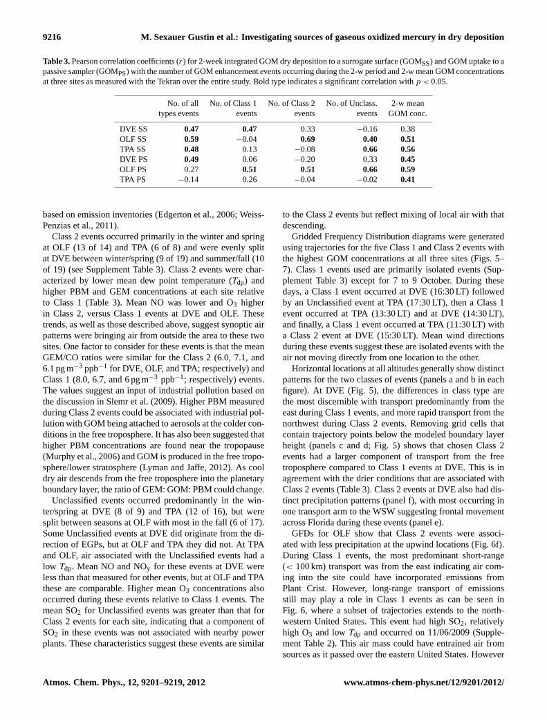
Table 3.Pearson correlation coefficients (r) for 2-week integrated GOM dry deposition to a surrogate surface (GOMSS) and GOM uptake to apassive sampler (GOMPS) with the number of GOM enhancement events occurring during the 2-w period and 2-w mean GOM concentrationsat three sites as measured with the Tekran over the entire study. Bold type indicates a significant correlation withp < 0.05.

No. of all No. of Class 1 No. of Class 2 No. of Unclass. 2-w meantypes events events events events GOM conc.

DVE SS 0.47 0.47 0.33 −0.16 0.38OLF SS 0.59 −0.04 0.69 0.40 0.51TPA SS 0.48 0.13 −0.08 0.66 0.56DVE PS 0.49 0.06 −0.20 0.33 0.45OLF PS 0.27 0.51 0.51 0.66 0.59TPA PS −0.14 0.26 −0.04 −0.02 0.41

based on emission inventories (Edgerton et al., 2006; Weiss-Penzias et al., 2011).

Class 2 events occurred primarily in the winter and springat OLF (13 of 14) and TPA (6 of 8) and were evenly splitat DVE between winter/spring (9 of 19) and summer/fall (10of 19) (see Supplement Table 3). Class 2 events were char-acterized by lower mean dew point temperature (Tdp) andhigher PBM and GEM concentrations at each site relativeto Class 1 (Table 3). Mean NO was lower and O3 higherin Class 2, versus Class 1 events at DVE and OLF. Thesetrends, as well as those described above, suggest synoptic airpatterns were bringing air from outside the area to these twosites. One factor to consider for these events is that the meanGEM/CO ratios were similar for the Class 2 (6.0, 7.1, and6.1 pg m−3 ppb−1 for DVE, OLF, and TPA; respectively) andClass 1 (8.0, 6.7, and 6 pg m−3 ppb−1; respectively) events.The values suggest an input of industrial pollution based onthe discussion in Slemr et al. (2009). Higher PBM measuredduring Class 2 events could be associated with industrial pol-lution with GOM being attached to aerosols at the colder con-ditions in the free troposphere. It has also been suggested thathigher PBM concentrations are found near the tropopause(Murphy et al., 2006) and GOM is produced in the free tropo-sphere/lower stratosphere (Lyman and Jaffe, 2012). As cooldry air descends from the free troposphere into the planetaryboundary layer, the ratio of GEM: GOM: PBM could change.

Unclassified events occurred predominantly in the win-ter/spring at DVE (8 of 9) and TPA (12 of 16), but weresplit between seasons at OLF with most in the fall (6 of 17).Some Unclassified events at DVE did originate from the di-rection of EGPs, but at OLF and TPA they did not. At TPAand OLF, air associated with the Unclassified events had alow Tdp. Mean NO and NOy for these events at DVE wereless than that measured for other events, but at OLF and TPAthese are comparable. Higher mean O3 concentrations alsooccurred during these events relative to Class 1 events. Themean SO2 for Unclassified events was greater than that forClass 2 events for each site, indicating that a component ofSO2 in these events was not associated with nearby powerplants. These characteristics suggest these events are similar

to the Class 2 events but reflect mixing of local air with thatdescending.

Gridded Frequency Distribution diagrams were generatedusing trajectories for the five Class 1 and Class 2 events withthe highest GOM concentrations at all three sites (Figs. 5–7). Class 1 events used are primarily isolated events (Sup-plement Table 3) except for 7 to 9 October. During thesedays, a Class 1 event occurred at DVE (16:30 LT) followedby an Unclassified event at TPA (17:30 LT), then a Class 1event occurred at TPA (13:30 LT) and at DVE (14:30 LT),and finally, a Class 1 event occurred at TPA (11:30 LT) witha Class 2 event at DVE (15:30 LT). Mean wind directionsduring these events suggest these are isolated events with theair not moving directly from one location to the other.

Horizontal locations at all altitudes generally show distinctpatterns for the two classes of events (panels a and b in eachfigure). At DVE (Fig. 5), the differences in class type arethe most discernible with transport predominantly from theeast during Class 1 events, and more rapid transport from thenorthwest during Class 2 events. Removing grid cells thatcontain trajectory points below the modeled boundary layerheight (panels c and d; Fig. 5) shows that chosen Class 2events had a larger component of transport from the freetroposphere compared to Class 1 events at DVE. This is inagreement with the drier conditions that are associated withClass 2 events (Table 3). Class 2 events at DVE also had dis-tinct precipitation patterns (panel f), with most occurring inone transport arm to the WSW suggesting frontal movementacross Florida during these events (panel e).

GFDs for OLF show that Class 2 events were associ-ated with less precipitation at the upwind locations (Fig. 6f).During Class 1 events, the most predominant short-range(< 100 km) transport was from the east indicating air com-ing into the site could have incorporated emissions fromPlant Crist. However, long-range transport of emissionsstill may play a role in Class 1 events as can be seen inFig. 6, where a subset of trajectories extends to the north-western United States. This event had high SO2, relativelyhigh O3 and lowTdp and occurred on 11/06/2009 (Supple-ment Table 2). This air mass could have entrained air fromsources as it passed over the eastern United States. However



the trajectories suggest the potential for longer range trans-port. The PBM during this event was also relatively high(8 pg m−3), as was NOy (12 ppb) and CO (185 ppb) suggest-ing an anthropogenic pollution component. The GFDs gener-ated for the TPA events do not point towards a specific sourcefor Class 1 events and the upper troposphere transport acrossthe United States is shown for Class 2 events (Fig. 7).

3.5 Analyses of event trends and data collected using theGOM passive sampler and surrogate surfaces

Comparing the number of Tekran® derived events withthe passive sampler uptake and surrogate surface depositionshows the best correlation for events recorded at OLF (Ta-ble 3). There is a good correlation between the GOMss de-position and the Class 2 and Unclassified events measured atthis location, however not for the Class 1 events. The onlyother correlations are for the GOMss deposition with num-ber of Class 1 events at DVE and with Unclassified eventsat TPA (Table 3). This indicates that either the passive sys-tems are not recording events or that the Tekran system asconfigured, is best measuring the form(s) of Hg (II) that areprevalent at OLF and not that at DVE and TPA.

4 Conclusions

Each site was different in terms of potential Hg inputs but ingeneral similar in local atmospheric chemistry with O3 highin the afternoon, CO, NOy, NO peaking in the morning, andall sites having a morning peak in SO2. Despite the similartrends, the magnitude of the peaks for Hg and other pollu-tants varies by site. OLF was the least impacted site withrespect to point and nonpoint sources. If the dry depositionmeasured in the summer at OLF represents a “natural back-ground” value for Florida (0.03 ng m−2 h−1), then depositionin the fall (as measured by the surrogate surfaces) was notsignificantly impacted by the nearby EGP because deposi-tion remained the same. Deposition at this site was highest inthe spring (0.11 ng m−2 h−1), and based on trajectory analy-ses in this paper and from previous work, this is due to inputsfrom outside of the local area and long range transport.

At TPA, deposition (mean annual 0.20 ng m−2 h−1) wasabove the assumed Florida background value, and mean sea-sonal values ranged from 0.16 to 0.24 ng m−2 h−1 for sum-mer to spring. The additional spring input, if compared tothe summer value, was 0.08 ng m−2 h−1 and similar to that atOLF. The higher values overall at TPA are attributed to lo-cal mobile source emissions facilitating GOM formation thatwas subsequently deposited.

At DVE seasonal deposition was lowest in the winter andsummer (0.11 and 0.13 ng m−2 h−1, respectively) and abovethe background value for Florida. Deposition was highest inthe fall and spring (0.25 and 0.22 ng m−2 h−1, respectively.The peak afternoon GOM concentrations were highest in the

fall when air was from the general direction of the waste-to energy facilities and thus, this facility is contributing ei-ther GOM or GEM that may be locally oxidized. This issupported by the fact that in winter traffic density is higher,deposition is lower, and the air was not derived from the di-rection of local EGPs. The lowest afternoon peak in GOMwas also observed in the winter when the air was not comingfrom these facilities.

Based on GOMss measured deposition, deposition veloci-ties developed using the surrogate surface data, and Tekran®

derived GOM concentrations, Peterson et al. (2012) sug-gested that the chemical forms of GOM varied between thesesites spatially and temporally. Annual deposition to the surro-gate surfaces at TPA and DVE were more than 2-fold greaterthan that measured OLF reflecting differences in chemistry,concentration and sources. This work showed that the collec-tive use of information developed during periods of dry de-position in Florida could help understand potential sourcesof Hg. However to allocate specific source contributions, thechemistry of the forms of Hg measured by the samplers andTekran® system must be understood.

Supplementary material related to this article isavailable online at:http://www.atmos-chem-phys.net/12/9201/2012/acp-12-9201-2012-supplement.pdf.

Acknowledgements.This research was funded by EPRI. Wethank the State of Florida and SEARCH personnel for deployingand shipping the samplers over the year of this study as well asmaintaining the sampling sites; compiling the automated systemdata presented; and for performing the QA and operating theseintensive monitoring sites. Special thanks to Melissa Markee andCassandra Woodward for making the trek to Florida to establishingthe field sites and coordinating the sampling and sample analyses.Much thanks to Musheng Alishahi who managed all aspects of thisproject and to Coty Weaver and Vanessa Wehrkamp for keepingthe sampler flow going. Thanks also to Arnout ter Shure and HenryFuelberg for review of this manuscript prior to submission.

Edited by: A. Dastoor

References

Amos, H. M., Jacob, D. J., Holmes, C. D., Fisher, J. A., Wang,Q., Yantosca, R. M., Corbitt, E. S., Galarneau, E., Rutter, A. P.,Gustin, M. S., Steffen, A., Schauer, J. J., Graydon, J. A., Louis,V. L. St., Talbot, R. W., Edgerton, E. S., Zhang, Y., and Sunder-land, E. M.: Gas-particle partitioning of atmospheric Hg(II) andits effect on global mercury deposition, Atmos. Chem. Phys., 12,591–603,doi:10.5194/acp-12-591-2012, 2012.

Ariya, P. A., Peterson, K., Snider, G., and Amyot, M.: Mercurychemical transformations in the gas, aqueous and heterogeneousphases: state-of-the-art science and uncertainties, in: Mercury


http://www.atmos-chem-phys.net/12/9201/2012/acp-12-9201-2012-supplement.pdf

http://www.atmos-chem-phys.net/12/9201/2012/acp-12-9201-2012-supplement.pdf

http://dx.doi.org/10.5194/acp-12-591-2012


Fate and Transport in the Global Atmosphere, edited by: Ma-son, R. and Pirrone, N., Spring Science+Business Median, NewYork, NY, USA, 2009.

Biswas, S., Verma, V., Schauer, J., Cassee, F., Cho, A., and Sioutas,C.: Oxidative potential of semivolatile and non volatile par-ticulate matter (PM) from heavy-duty vehicles retrofitted withemission control technologies, Environ. Sci. Technol., 43, 3905–3912, 2009.

Butler, T. J., Cohen, M. D., Vermeylen, F. M., Likens, G. E.,Schmeltz, D., and Artz, R. S.: Regional precipitation mercurytrends in the eastern USA, 1998–2005: Declines in the Northeatand Midwest, no trend in the Southeast, Atmos. Environ., 42,1582–1592, 2008.

Calvert, J. G. and Lindberg, S. E.: Mechanisms of mercury removalby O-3 and OH in the atmosphere, Atmos. Environ., 39, 3355–3367, 2005.

Castro, M. S., Moore, C., Sherwell, J., And Brooks, S. B.: Dry de-position of gaseous oxidized mercury in Western Maryland, Sci.Total Environ., 417, 232–240, 2012.

Draxler, R. R. and Hess, G. D.: Description of the HYSPLIT – 4modeling system, NOAA Tech. Memo., ERL ARL-224, 24 pp.,1997.

Dvonch, J. T., Graney, J. R., Keeler, G. J., and Stevens, R. K.: Useof elemental tracers to source apportion mercury in South Floridaprecipitation, Environ. Sci. Technol., 24, 4522–4527, 1999.

Dvonch, J. G., Keeler, G. J., and Marsik, F. J.: The influence ofmeteorological conditions on the wet deposition of mercury insouthern Florida, J. App. Meteorol., 44, 1421–1435, 2005.

Edgerton, E. S., Hartsell, B. E., and Jansen, J. J.: Mercury speciationin coal-fired power plant plumes observed at three surface sitesin the southeastern U.S., Environ. Sci. Technol., 40, 4563–4570,2006.

Engle, M. A., Tate, M. T., Krabbenhoft, D. P., Kolker, Allan, Olson,M. L., Edgerton, E. S., DeWild, J. F., and McPherson, A. K.:Characterization and cycling of atmospheric mercury along thecentral U.S. Gulf Coast, Appl. Geochem., 23, 419–437, 2008.

Engle, M. A., Tate, M. T., Krabbenhoft, D. P., Schauer, J. J., Kolker,A., Shanley, J. B., and Bothner, M. H.: Comparison of atmo-spheric mercury speciation and deposition at nine sites acrosscentral and eastern North America, J. Geophys. Res.-Atmos.,115, D18306,doi:10.1029/2010JD014064, 2010.

Feng, X., Lu, J. Y., Gregoire, C., Hao, Y., Banic, C. M., andSchroeder, W.: Analysis of inorganic mercury species associatedwith airborne particulate matter/aerosols: method development,Anal. Bioanal. Chem., 380, 683–689, 2004.

Finlayson-Pitts, B. J. and Pitts, J. N.: Chemistry of the Upper andLower Atmosphere, Academic Press, San Diego, CA, USA, 969pp., 2000.

Guentzel, J. L., Landing, W. M., Gill, G. A., and Pollman, C. D.:Processes influencing rainfall deposition of mercury in Florida,Environ. Sci. Technol., 35, 863–873, 2001.

Gustin, M. S. and Jaffe, D.: Reducing the uncertainty in measure-ment and understanding of mercury in the atmosphere, Environ.Sci. Technol., 44, 2222–2227, 2010.

Gustin, M. S.: Exchange of Mercury between the Atmosphere andTerrestrial Ecosystems, in: Environmental Chemistry and Toxi-cology of Mercury, edited by: Liu, G., Cai, Y., and O’Driscoll,N., John Wiley and Sons, 423–454, 2012.

Gustin, M. S., Lyman, S. N., Kilner, P., and Prestbo, E.: Develop-ment of a passive sampler for gaseous mercury, Atmos. Environ.,45, 5805–5812, 2011.

Holmes, C. D., Jacob, D. J., Corbitt, E. S., Mao, J., Yang, X., Tal-bot, R., and Slemr, F.: Global atmospheric model for mercuryincluding oxidation by bromine atoms, Atmos. Chem. Phys., 10,12037–12057,doi:10.5194/acp-10-12037-2010, 2010.

Hynes, A. J., Donohoue, D. L., Goodsite, M. E., and Hedgecock,I. M.: Our current understanding of major chemical and physi-cal processes affecting mercury dynamics in the atmosphere andat the air-water/terrestrial interfaces, edited by: Mason, R., andPirrone, N., in: Mercury Fate and Transport in the Global Atmo-sphere, Spring Science+Business Media, New York, NY, USA,2009.

Landing, W. M., Caffrey, J. M., Nolek, S. D., Gosnell, K. J., andParker, W. C.: Atmospheric wet deposition of mercury and othertrace elements in Pensacola, Florida, Atmos. Chem. Phys., 10,4867–4877,doi:10.5194/acp-10-4867-2010, 2010.

Lin, C.-J., Pongprueksa, P., Lindberg, S. E., Pehkonen, S. O., Byun,D., and Jang, C.: Scientific uncertainties in atmospheric mercurymodels 1: model science evaluation, Atmos. Environ., 40, 2067–2079, 2006.

Lindberg, S. E. and Stratton, W. J.: Atmospheric speciation concen-trations and behavior of reactive gaseous mercury in ambient air,Environ. Sci. Technol., 32, 49–57, 1998.

Lohman, K., Seigneur, C., Edgerton, E. S., and Jansen, J. J.: Mod-eling mercury in power plant plumes, Environ. Sci. Technol., 40,3848–3854, 2006.

Lyman, S. and Gustin, M. S.: Determinants of Atmospheric Mer-cury Concentrations in Reno, Nevada, U.S.A., Sci. Total. Envi-ron., 408, 431–438, 2009.

Lyman, S. N. and Jaffe, D. A.: Formation and fate of oxidized mer-cury in the upper troposphere and lower stratosphere, NatureGeosci., 5, 114–117, 2012.

Lyman, S. N., Gustin, M. S., Prestbo, E. M., and Marsick, F. J.: Esti-mation of Dry Deposition of Atmospheric Mercury in Nevada byDirect and Indirect Methods, Environ. Sci. Technol., 41, 1970–1976, 2007.

Lyman, S. N., Gustin, M. S., Prestbo, E. M., Kilner, P. I., Edger-ton, E., and Hartsell, B.: Testing and Application of SurrogateSurfaces for Understanding Potential Gaseous Oxidized MercuryDry Deposition, Environ. Sci. Technol., 43, 6235–6241, 2009.

Lyman, S., Gustin, M. S., and Prestbo, E.: Development and use ofpassive samplers for determining reactive gaseous mercury con-centrations, Atmos. Environ., 44, 246–252, 2010.

Marsik, F. J., Keeler, G. J., and Landis, M. S.: The dry-deposition ofspeciated mercury to the Florida Everglades: Measurements andmodeling, Atmos. Environ., 41, 136–149, 2007.

Murphy, D. M., Hudson, P. K., Thomson, D. S., Sheridan, P. J.,and Wilson, J. C.: Observations of mercury-containing aerosols,Environ. Sci. Technol., 40, 3163–3167, 2006.

National Atmospheric Deposition Program. Mercury DepositionNetwork (MDN): A NADP network. NADP Program Office, Illi-nois State Water Survey, Champaign, IL,http://nadp.sws.uiuc.edu/mdn/, (last access: 23 January 2012), 2012.

Pal, B. and Ariya, P. A.: Gas-phase HO center dot-initiated reactionsof elemental mercury: Kinetics, product studies and atmosphericimplications, Environ. Sci. Technol., 38, 5555–5566, 2004.


http://dx.doi.org/10.1029/2010JD014064



http://nadp.sws.uiuc.edu/mdn/

http://nadp.sws.uiuc.edu/mdn/


Peterson, C., Gustin, M., and Lyman, S.: Atmospheric mercury con-centrations and speciation measured from 2004 to 2007 in Reno,Nevada, USA, Atmos. Environ., 30, 4646–4654, 2009.

Peterson, C., Alishahi, M., and Gustin, M. S.: Testing the use ofpassive sampling systems for understanding air mercury concen-trations and dry deposition across Florida, USA, Sci. Total Envi-ron., 424, 297–309, 2012.

Prestbo, E. M. and Gay, D. A.: Wet deposition of mercury inthe U.S. and Canada, 1996–2005: results and analysis of theNADP Mercury Deposition Network (MDN), Atmos. Environ.,43, 4223–4233, 2009.

Schroeder, W. H. and Munthe, J.: Atmospheric mercury – Anoverview, Atmos. Environ. 32, 809–822, 1998.

Seigneur, C., Wrobel., J., and Constantinou, E.: A chemical ki-netic mechanism for atmospheric inorganic mercury, Environ.Sci. Technol., 28, 1589–1597, 1994.

Selin, N. E. and Jacob, D. J.: Seasonal and spatial patterns of mer-cury wet deposition in the United States: Constraints on the con-tribution from North American anthropogenic sources, Atmos.Environ., 42, 5193–5204, 2008.

Sillman, S., Marsik, F. J., Al-Wali, K. I., Keeler, G. J., andLandis, M. S.: Reactive mercury in the troposphere: Modelformation and results for Florida, the northeastern UnitedStates, and the Atlantic Ocean, J. Geophys. Res., 112, D23305,doi:10.1029/2006JD008227, 2007.

Slemr, F., Ebinghaus, R., Brenninkmeijer, C.A. M., Hermann, M.,Kock, H. H., Martinsson, B. G., Shuck, T., Sprung, D., vanVelthoven, P., Zahn, A., and Ziereis, H.: Gaseous mercury distri-bution in the upper troposphere and lower stratosphere observedonboard the CARIBIC passenger aircraft, Atmos. Chem. Phys.,9, 1957–1969,doi:10.5194/acp-9-1957-2009, 2009.

Steffen, A., Scherz, T., Olson, M., Gay, D., and Blanchard, P.: Com-parison of data quality control protocols for atmospheric specia-tion measurements, J. Environ. Monitor., 14, 752–765, 2012.

Stohl, A.: Computation, accuracy and applications of trajectories –a review and bibliography, Atmos. Environ., 32, 947–966, 1998.

Stohl, A., Forster, C., Eckhardt, S., Spichtinger, N., Huntrieser, H.,Heland, J., Schlager, H., Wilhelm, S., Arnold, F., and Cooper, O.:A backward modeling study of intercontinental pollution trans-port using aircraft measurements, J. Geophys. Res., 108, 4370,doi:10.1029/2002JD002862, 2003.

Subir, M., Ariya, P. A., and Dastoor, A. P.: A review of the uncer-tainties in atmospheric modeling of mercury chemistry I. Uncer-tainties in existing kinetic parameters : Fundamental limitationsand the importance of heterogeneous chemistry, Atmos. Envi-ron., 35, 5667–5676, 2011.

Subir, M., Ariya, P. A., and Dastoor, A. P.: A review of the sourcesof uncertainties in atmospheric mercury modeling II. Mercurysurface and heterogeneous chemistry – A missing link, Atmos.Environ., 46, 1–10, 2012.

Weiss-Penzias, S., Gustin, M. S., and Lyman, S. N.: Obser-vations of speciated atmospheric mercury at three sites inNevada, USA: Evidence for a free tropospheric source ofreactive gaseous mercury, J. Geophys. Res., 114, D14302,doi:10.1029/2008JD011607, 2009.

Weiss-Penzias, P. S., Gustin, M. S., and Lyman, S. N.: Sources ofgaseous oxidized mercury and mercury dry deposition at twosoutheastern US sites, Atmos. Environ., 45, 4569–4579, 2011.

Wesley, M. L.: Parameterization of surface resistances to gaseousdry deposition in regional-scale numerical models, Atmos. Env-iron., 34, 2261–2282, 1989.

Zhang, L., Blanchard, P., Gay, D. A., Prestbo, E. M., Risch, M. R.,Johnson, D., Narayan, J., Zsolway, R., Holsen, T. M., Miller, E.K., Castro, M. S., Graydon, V. L., Dalziel, J.: Estimation of spe-ciated and total mercury dry deposition at monitoring locationsin eastern and central North America. Atmos. Chem. Phys. 12,4327–4340,doi:10.5194/acp-12-4327-2012, 2012.


http://dx.doi.org/10.1029/2006JD008227


http://dx.doi.org/10.1029/2002JD002862

http://dx.doi.org/10.1029/2008JD011607


investigating sources of gaseous oxidized mercury in dry deposition

Documents