investigating the impact of adaptation sampling in natural...
TRANSCRIPT
Investigating the Impact of Adaptation Sampling in NaturalEvolution Strategies on Black-box Optimization Testbeds
Tom SchaulCourant Institute of Mathematical Sciences, New York University
Broadway 715, New York, [email protected]
ABSTRACTNatural Evolution Strategies (NES) are a recent memberof the class of real-valued optimization algorithms that arebased on adapting search distributions. Exponential NES(xNES) are the most common instantiation of NES, andparticularly appropriate for the BBOB 2012 benchmarks,given that many are non-separable, and their relatively smallproblem dimensions. The technique of adaptation sampling,which adapts learning rates online further improves the al-gorithm’s performance. This report provides an extensiveempirical comparison to study the impact of adaptationsampling in xNES, both on the noise-free and noisy BBOBtestbeds.
Categories and Subject DescriptorsG.1.6 [Numerical Analysis]: Optimization—global opti-mization, unconstrained optimization; F.2.1 [Analysis ofAlgorithms and Problem Complexity]: Numerical Al-gorithms and Problems
General TermsAlgorithms
KeywordsEvolution Strategies, Natural Gradient, Benchmarking
1. INTRODUCTIONEvolution strategies (ES), in contrast to traditional evo-
lutionary algorithms, aim at repeating the type of muta-tion that led to those good individuals. We can characterizethose mutations by an explicitly parameterized search dis-tribution from which new candidate samples are drawn, akinto estimation of distribution algorithms (EDA). Covariancematrix adaptation ES (CMA-ES [10]) innovated the field byintroducing a parameterization that includes the full covari-ance matrix, allowing them to solve highly non-separableproblems.
Permission to make digital or hard copies of all or part of this work forpersonal or classroom use is granted without fee provided that copies arenot made or distributed for profit or commercial advantage and that copiesbear this notice and the full citation on the first page. To copy otherwise, torepublish, to post on servers or to redistribute to lists, requires prior specificpermission and/or a fee.GECCO’12 Companion, July 7–11, 2012, Philadelphia, PA, USA.Copyright 2012 ACM 978-1-4503-1178-6/12/07 ...$10.00.
A more recent variant, natural evolution strategies (NES [20,6, 18, 19]) aims at a higher level of generality, providing aprocedure to update the search distribution’s parameters forany type of distribution, by ascending the gradient towardshigher expected fitness. Further, it has been shown [15, 12]that following the natural gradient to adapt the search dis-tribution is highly beneficial, because it appropriately nor-malizes the update step with respect to its uncertainty andmakes the algorithm scale-invariant.
Exponential NES (xNES), the most common instantiationof NES, used a search distribution parameterized by a meanvector and a full covariance matrix, and is thus most sim-ilar to CMA-ES (in fact, the precise relation is describedin [4] and [5]). Given the relatively small problem dimen-sions of the BBOB benchmarks, and the fact that many arenon-separable, it is also among the most appropriate NESvariants for the task.
Adaptation sampling (AS) is a technique for the onlineadaptation of its learning rate, which is designed to speedup convergence. This may be beneficial to algorithms likexNES, because the optimization traverses qualitatively dif-ferent phases, during which different learning rates may beoptimal.
In this report, we retain the original formulation of xNES(including all parameter settings, except for an added stop-ping criterion), and compare this base-line algorithm withan AS-augmented variant. We describe the empirical perfor-mance on all 54 benchmark functions (both noise-free andnoisy) of the BBOB 2012 workshop.
2. NATURAL EVOLUTION STRATEGIESNatural evolution strategies (NES) maintain a search dis-
tribution π and adapt the distribution parameters θ by fol-lowing the natural gradient [1] of expected fitness J , that is,maximizing
J(θ) = Eθ[f(z)] =
∫f(z) π(z | θ) dz
Just like their close relative CMA-ES [10], NES algorithmsare invariant under monotone transformations of the fit-ness function and linear transformations of the search space.Each iteration the algorithm produces n samples zi ∼ π(z|θ),i ∈ {1, . . . , n}, i.i.d. from its search distribution, which is pa-rameterized by θ. The gradient w.r.t. the parameters θ canbe rewritten (see [20]) as
∇θJ(θ) = ∇θ∫f(z) π(z | θ) dz = Eθ [f(z) ∇θ log π(z | θ)]
221
from which we obtain a Monte Carlo estimate
∇θJ(θ) ≈ 1
n
n∑i=1
f(zi) ∇θ log π(zi | θ)
of the search gradient. The key step then consists in replac-ing this gradient by the natural gradient defined as F−1∇θJ(θ)
where F = E[∇θ log π (z|θ)∇θ log π (z|θ)>
]is the Fisher
information matrix. The search distribution is iterativelyupdated using natural gradient ascent
θ ← θ + ηF−1∇θJ(θ)
with learning rate parameter η.
2.1 Exponential NESWhile the NES formulation is applicable to arbitrary pa-
rameterizable search distributions [20, 12], the most com-mon variant employs multinormal search distributions. Forthat case, two helpful techniques were introduced in [6],namely an exponential parameterization of the covariancematrix, which guarantees positive-definiteness, and a novelmethod for changing the coordinate system into a “natural”one, which makes the algorithm computationally efficient.The resulting algorithm, NES with a multivariate Gaussiansearch distribution and using both these techniques is calledxNES, and the pseudocode is given in Algorithm 1.
Algorithm 1: Exponential NES (xNES)
input: f , µinit, ησ, ηB, uk
initializeµ ← µinit
σ ← 1B ← I
repeatfor k = 1 . . . n do
draw sample sk ∼ N (0, I)zk ← µ + σB>skevaluate the fitness f(zk)
end
sort {(sk, zk)} with respect to f(zk)and assign utilities uk to each sample
compute gradients∇δJ ←
∑nk=1 uk · sk
∇MJ ←∑nk=1 uk · (sks
>k − I)
∇σJ ← tr(∇MJ)/d∇BJ ← ∇MJ −∇σJ · I
update parametersµ ← µ + σB · ∇δJσ ← σ · exp(ησ/2 · ∇σJ)B ← B · exp(ηB/2 · ∇BJ)
until stopping criterion is met
2.2 Adaptation SamplingFirst introduced in [12] (chapter 2, section 4.4), adapta-
tion sampling is a new meta-learning technique [17] that canadapt hyper-parameters online, in an economical way thatis grounded on a measure statistical improvement.
Here, we apply it to the learning rate of the global step-size ησ. The idea is to consider whether a larger learning-
rate η′σ = 32ησ would have been more likely to generate the
good samples in the current batch. For this we determinethe (hypothetical) search distribution that would have re-sulted from such a larger update π(·|θ′). Then we computeimportance weights
w′k =π(zk|θ′)π(zk|θ)
for each of the n samples zk in our current population, gen-erated from the actual search distribution π(·|θ). We thenconduct a weighted Mann-Whitney test [12] (appendix A) todetermine if the set {rank(zk)} is inferior to its reweightedcounterpart {w′k · rank(zk)} (corresponding to the largerlearning rate), with statistical significance ρ. If so, we in-crease the learning rate by a factor of 1 + c′, up to at mostησ = 1 (where c′ = 0.1). Otherwise it decays to its initialvalue:
ησ ← (1− c′) · ησ + c′ · ησ,init
The procedure is summarized in algorithm 2 (for details andderivations, see [12]). The combination of xNES with adap-tation sampling is dubbed xNES-as.
One interpretation of why adaptation sampling is helpfulis that half-way into the search, (after a local attractor hasbeen found, e.g., towards the end of the valley on the Rosen-brock benchmarks f8 or f9), the convergence speed can beboosted by an increased learning rate. For such situations,an online adaptation of hyper-parameters is inherently well-suited.
Algorithm 2: Adaptation sampling
input : ησ,t,ησ,init, θt, θt−1, {(zk, f(zk))}, c′, ρoutput: ησ,t+1
compute hypothetical θ′, given θt−1 and using 3/2ησ,tfor k = 1 . . . n do
w′k =π(zk|θ′)π(zk|θ)
endS ← {rank(zk)}S′ ← {w′k · rank(zk)}if weighted-Mann-Whitney(S, S′) < ρ then
return (1− c′) · ησ + c′ · ησ,initelse
return min((1 + c′) · ησ, 1)end
3. EXPERIMENTAL SETTINGSWe use identical default hyper-parameter values for all
benchmarks (both noisy and noise-free functions), whichare taken from [6, 12]. Table 1 summarizes all the hyper-parameters used.
In addition, we make use of the provided target fitness foptto trigger independent algorithm restarts1, using a simplead-hoc procedure: If the log-progress during the past 1000d
1It turns out that this use of fopt is technically not permit-ted by the BBOB guidelines, so strictly speaking a differentrestart strategy should be employed, for example the onedescribed in [12].
222
Table 1: Default parameter values for xNES (includ-ing the utility function and adaptation sampling) asa function of problem dimension d.
parameter default value
n 4 + b3 log(d)c
ησ = ηB3(3 + log(d))
5d√d
ukmax
(0, log(n
2+ 1)− log(k)
)∑nj=1 max
(0, log(n
2+ 1)− log(j)
) − 1
n
ρ1
2− 1
3(d+ 1)
c′1
10
evaluations is too small, i.e., if
log10
∣∣∣∣ fopt − ftfopt − ft−1000d
∣∣∣∣ < (r+2)2 ·m3/2 · [log10 |fopt−ft|+8]
where m is the remaining budget of evaluations divided by1000d, ft is the best fitness encountered until evaluation tand r is the number of restarts so far. The total budget is105d3/2 evaluations.
Implementations of this and other NES algorithm vari-ants are available in Python through the PyBrain machinelearning library [16], as well as in other languages at www.
idsia.ch/~tom/nes.html.
4. RESULTSResults from experiments according to [7] on the bench-
mark functions given in [2, 8, 3, 9] are presented in Figures 1,2 and 3, and in Tables 2, 3 and 4. The expected runningtime (ERT), used in the figures and table, depends on agiven target function value, ft = fopt+∆f , and is computedover all relevant trials as the number of function evaluationsexecuted during each trial while the best function value didnot reach ft, summed over all trials and divided by the num-ber of trials that actually reached ft [7, 11]. Statisticalsignificance is tested with the rank-sum test for a giventarget ∆ft (10−8 using, for each trial, either the number ofneeded function evaluations to reach ∆ft (inverted and mul-tiplied by −1), or, if the target was not reached, the best∆f -value achieved, measured only up to the smallest num-ber of overall function evaluations for any unsuccessful trialunder consideration.
Some of the result plots (like performance scaling withdimension), as well as the CPU-timing results were omit-ted here but are available in stand-alone benchmarking re-ports [14, 13].
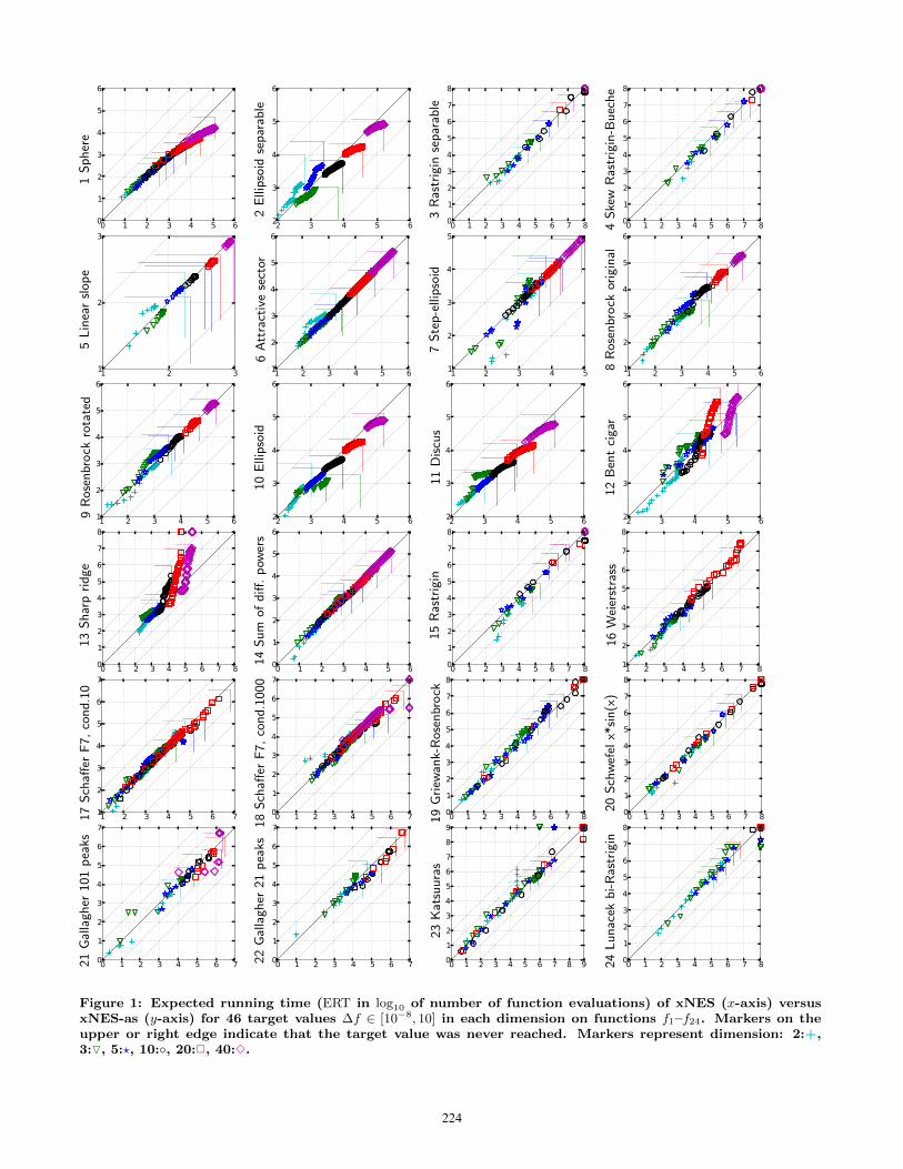
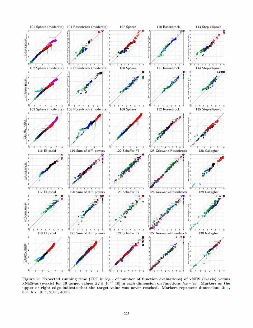
5. DISCUSSIONNaturally, the core algorithm (xNES) being identical in
both variants presented here, we do not expect drasticallydifferent results. In fact, the direct comparison Figures 1and 2 show remarkably similar results on the majority offunctions, which we see from the points clearly scatteredalong the diagonal. This indicates that on most benchmarks,
adaptation sampling is not used (much) and xNES-as oper-ates with the same conservative learning rates as xNES.
The functions where we observe differences are telling,however. Most notably on the sphere function (f1, andits noisy siblings), adaptation sampling drastically improvesperformance, by up to a factor 4. Adaptation sampling stillimproves performance significantly on many other functions(see Table 2), but the speed-ups are less striking. Thereis a single function where adaptation sampling significantlyhurts performance, namely on f13 in dimension 20 (the sharpridge): apparently the learning rates are increased to anoverly aggressive level.
In conclusion, we can recommend using adaptation sam-pling for xNES in general, and particularly so if the fitnesslandscapes are smooth.
AcknowlegementsThe author wants to thank the organizers of the BBOBworkshop for providing such a well-designed benchmark setup,and especially such high-quality post-processing utilities.
This work was funded in part through AFR postdoc grantnumber 2915104, of the National Research Fund Luxem-bourg.
6. REFERENCES[1] S. I. Amari. Natural Gradient Works Efficiently in
Learning. Neural Computation, 10:251–276, 1998.
[2] S. Finck, N. Hansen, R. Ros, and A. Auger.Real-parameter black-box optimization benchmarking2009: Presentation of the noiseless functions.Technical Report 2009/20, Research Center PPE,2009. Updated February 2010.
[3] S. Finck, N. Hansen, R. Ros, and A. Auger.Real-parameter black-box optimization benchmarking2010: Presentation of the noisy functions. TechnicalReport 2009/21, Research Center PPE, 2010.
[4] N. Fukushima, Y. Nagata, S. Kobayashi, and I. Ono.Proposal of distance-weighted exponential naturalevolution strategies. In 2011 IEEE Congress ofEvolutionary Computation, pages 164–171. IEEE,2011.
[5] T. Glasmachers, T. Schaul, and J. Schmidhuber. ANatural Evolution Strategy for Multi-ObjectiveOptimization. In Parallel Problem Solving from Nature(PPSN), 2010.
[6] T. Glasmachers, T. Schaul, Y. Sun, D. Wierstra, andJ. Schmidhuber. Exponential Natural EvolutionStrategies. In Genetic and Evolutionary ComputationConference (GECCO), Portland, OR, 2010.
[7] N. Hansen, A. Auger, S. Finck, and R. Ros.Real-parameter black-box optimization benchmarking2012: Experimental setup. Technical report, INRIA,2012.
[8] N. Hansen, S. Finck, R. Ros, and A. Auger.Real-parameter black-box optimization benchmarking2009: Noiseless functions definitions. Technical ReportRR-6829, INRIA, 2009. Updated February 2010.
[9] N. Hansen, S. Finck, R. Ros, and A. Auger.Real-parameter black-box optimization benchmarking2009: Noisy functions definitions. Technical ReportRR-6869, INRIA, 2009. Updated February 2010.
223
1S
ph
ere
0 1 2 3 4 5 60
1
2
3
4
5
61 S
phere
2E
llip
soid
sep
arab
le
2 3 4 5 62
3
4
5
6
2 E
llipso
id s
epara
ble
3R
astr
igin
sep
arab
le
0 1 2 3 4 5 6 7 80
1
2
3
4
5
6
7
8
3 R
ast
rigin
separa
ble
4S
kew
Ras
trig
in-B
uec
he
0 1 2 3 4 5 6 7 80
1
2
3
4
5
6
7
8
4 S
kew
Rast
rigin
-Buech
e s
epar
5L
inea
rsl
op
e
1 2 31
2
3
5 L
inear
slope
6A
ttra
ctiv
ese
ctor
1 2 3 4 5 61
2
3
4
5
6
6 A
ttra
ctiv
e s
ect
or
7S
tep
-elli
pso
id
1 2 3 4 51
2
3
4
5
7 S
tep-e
llipso
id
8R
ose
nbr
ock
orig
inal
1 2 3 4 5 61
2
3
4
5
6
8 R
ose
nbro
ck o
rigin
al
9R
ose
nbr
ock
rota
ted
1 2 3 4 5 61
2
3
4
5
6
9 R
ose
nbro
ck r
ota
ted
10
Elli
pso
id
2 3 4 5 62
3
4
5
6
10 E
llipso
id
11
Dis
cus
2 3 4 5 62
3
4
5
6
11 D
iscu
s
12
Ben
tci
gar
2 3 4 5 62
3
4
5
6
12 B
ent
cigar
13
Sh
arp
rid
ge
0 1 2 3 4 5 6 7 80
1
2
3
4
5
6
7
8
13 S
harp
rid
ge
14
Su
mo
fd
iff.
pow
ers
0 1 2 3 4 5 60
1
2
3
4
5
6
14 S
um
of
diffe
rent
pow
ers
15
Ras
trig
in
0 1 2 3 4 5 6 7 80
1
2
3
4
5
6
7
8
15 R
ast
rigin
16
Wei
erst
rass
1 2 3 4 5 6 7 81
2
3
4
5
6
7
8
16 W
eie
rstr
ass
17
Sch
affer
F7
,co
nd
.10
1 2 3 4 5 6 71
2
3
4
5
6
7
17 S
chaff
er
F7, co
ndit
ion 1
0
18
Sch
affer
F7
,co
nd
.10
00
0 1 2 3 4 5 6 70
1
2
3
4
5
6
7
18 S
chaff
er
F7, co
ndit
ion 1
000
19
Gri
ewan
k-R
ose
nbr
ock
0 1 2 3 4 5 6 7 80
1
2
3
4
5
6
7
8
19 G
riew
ank-
Rose
nbro
ck F
8F2
20
Sch
wef
elx*
sin
(x)
0 1 2 3 4 5 6 7 80
1
2
3
4
5
6
7
8
20 S
chw
efe
l x*s
in(x
)
21
Gal
lag
her
10
1p
eaks
0 1 2 3 4 5 6 70
1
2
3
4
5
6
7
21 G
alla
gher
101 p
eaks
22
Gal
lag
her
21
pea
ks
0 1 2 3 4 5 6 70
1
2
3
4
5
6
7
22 G
alla
gher
21 p
eaks
23
Kat
suu
ras
0 1 2 3 4 5 6 7 8 90
1
2
3
4
5
6
7
8
9
23 K
ats
uura
s
24
Lu
nac
ekb
i-R
astr
igin
0 1 2 3 4 5 6 7 80
1
2
3
4
5
6
7
8
24 L
unace
k bi-
Rast
rigin
Figure 1: Expected running time (ERT in log10 of number of function evaluations) of xNES (x-axis) versusxNES-as (y-axis) for 46 target values ∆f ∈ [10−8, 10] in each dimension on functions f1–f24. Markers on theupper or right edge indicate that the target value was never reached. Markers represent dimension: 2:+,3:O, 5:?, 10:◦, 20:2, 40:3.
224
101 Sphere (moderate) 104 Rosenbrock (moderate) 107 Sphere 110 Rosenbrock 113 Step-ellipsoidG
au
ssn
ois
e
1 2 3 4 5 61
2
3
4
5
6
101 S
phere
modera
te G
auss
0 1 2 3 4 5 6 7 80
1
2
3
4
5
6
7
8
104 R
ose
nbro
ck m
odera
te G
auss
0 1 2 3 4 5 6 7 8 90
1
2
3
4
5
6
7
8
9
107 S
phere
Gauss
0 1 2 3 4 5 6 7 80
1
2
3
4
5
6
7
8
110 R
ose
nbro
ck G
auss
0 1 2 3 4 5 6 7 8 90
1
2
3
4
5
6
7
8
9
113 S
tep-e
llipso
id G
auss
102 Sphere (moderate) 105 Rosenbrock (moderate) 108 Sphere 111 Rosenbrock 114 Step-ellipsoid
un
ifor
mn
ois
e
0 1 2 3 4 5 60
1
2
3
4
5
6
102 S
phere
modera
te u
nif
0 1 2 3 4 5 6 70
1
2
3
4
5
6
7
105 R
ose
nbro
ck m
odera
te u
nif
0 1 2 3 4 5 6 7 80
1
2
3
4
5
6
7
8
108 S
phere
unif
0 1 2 3 4 5 6 7 80
1
2
3
4
5
6
7
8
111 R
ose
nbro
ck u
nif
0 1 2 3 4 5 6 7 80
1
2
3
4
5
6
7
8
114 S
tep-e
llipso
id u
nif
103 Sphere (moderate) 106 Rosenbrock (moderate) 109 Sphere 112 Rosenbrock 115 Step-ellipsoid
Ca
uch
yn
ois
e
0 1 2 3 4 5 60
1
2
3
4
5
6
103 S
phere
modera
te C
auch
y
1 2 3 4 51
2
3
4
5
106 R
ose
nbro
ck m
odera
te C
auch
y
0 1 2 3 4 50
1
2
3
4
5
109 S
phere
Cauch
y
0 1 2 3 4 5 6 7 8 90
1
2
3
4
5
6
7
8
9
112 R
ose
nbro
ck C
auch
y1 2 3 4 5 61
2
3
4
5
6
115 S
tep-e
llipso
id C
auch
y
116 Ellipsoid 119 Sum of diff. powers 122 Schaffer F7 125 Griewank-Rosenbrock 128 Gallagher
Ga
uss
no
ise
0 1 2 3 4 5 6 7 8 90
1
2
3
4
5
6
7
8
9
116 E
llipso
id G
auss
0 1 2 3 4 5 6 7 8 90
1
2
3
4
5
6
7
8
9
119 S
um
of
diff
pow
ers
Gauss
0 1 2 3 4 5 6 7 80
1
2
3
4
5
6
7
8
122 S
chaff
er
F7 G
auss
0 1 2 3 4 5 6 7 80
1
2
3
4
5
6
7
8
125 G
riew
ank-
Rose
nbro
ck G
auss
0 1 2 3 4 5 6 7 80
1
2
3
4
5
6
7
8
128 G
alla
gher
Gauss
117 Ellipsoid 120 Sum of diff. powers 123 Schaffer F7 126 Griewank-Rosenbrock 129 Gallagher
un
ifor
mn
ois
e
0 1 2 3 4 5 6 7 80
1
2
3
4
5
6
7
8
117 E
llipso
id u
nif
0 1 2 3 4 5 6 7 80
1
2
3
4
5
6
7
8
120 S
um
of
diff
pow
ers
unif
0 1 2 3 4 5 6 7 80
1
2
3
4
5
6
7
8
123 S
chaff
er
F7 u
nif
0 1 2 3 4 5 6 7 80
1
2
3
4
5
6
7
8
126 G
riew
ank-
Rose
nbro
ck u
nif
0 1 2 3 4 5 6 7 80
1
2
3
4
5
6
7
8
129 G
alla
gher
unif
118 Ellipsoid 121 Sum of diff. powers 124 Schaffer F7 127 Griewank-Rosenbrock 130 Gallagher
Ca
uch
yn
ois
e
1 2 3 4 5 61
2
3
4
5
6
118 E
llipso
id C
auch
y
0 1 2 3 4 5 60
1
2
3
4
5
6
121 S
um
of
diff
pow
ers
Cauch
y
0 1 2 3 4 5 6 7 8 90
1
2
3
4
5
6
7
8
9
124 S
chaff
er
F7 C
auch
y
0 1 2 3 4 5 6 7 8 90
1
2
3
4
5
6
7
8
9
127 G
riew
ank-
Rose
nbro
ck C
auch
y
0 1 2 3 4 5 6 70
1
2
3
4
5
6
7
130 G
alla
gher
Cauch
y
Figure 2: Expected running time (ERT in log10 of number of function evaluations) of xNES (x-axis) versusxNES-as (y-axis) for 46 target values ∆f ∈ [10−8, 10] in each dimension on functions f101–f130. Markers on theupper or right edge indicate that the target value was never reached. Markers represent dimension: 2:+,3:O, 5:?, 10:◦, 20:2, 40:3.
225
5-D 20-D
∆f 1e+1 1e-1 1e-3 1e-5 1e-7 #succ
f1 11 12 12 12 12 15/151: xNES 3.0(3) 21(3) 50(6) 81(8) 110(7) 15/15
2: +as 2.9(2) 16(5) 37(8)?2 60(12)?3 78(17)?3 15/15
f2 83 88 90 92 94 15/151: xNES 8.7(2) 12(1) 16(1) 20(1) 23(1) 15/152: +as 11(5) 19(18) 39(62) 43(63) 49(92) 15/15
f3 716 1637 1646 1650 1654 15/151: xNES 3.0(1) 414(470) 412(489) 412(444) 411(440) 9/152: +as 1.5(0.7) 454(375) 452(459) 451(383) 450(364) 13/15
f4 809 1688 1817 1886 1903 15/151: xNES 4.5(6) 5871(6803) 5453(5586) 5255(5732) 5208(5693) 1/152: +as 3.8(5) 9998(10379) 9287(10842) 8949(9482) 8868(9550) 1/15
f5 10 10 10 10 10 15/151: xNES 9.5(4) 15(6) 16(6) 16(6) 16(6) 15/152: +as 10(4) 16(9) 16(8) 16(8) 16(8) 15/15
f6 114 281 580 1038 1332 15/151: xNES 1.6(1) 2.5(0.3) 2.2(0.3) 1.8(0.1) 1.8(0.1) 15/15
2: +as 1.5(1) 2.4(0.6) 2.0(0.2) 1.5(0.2)? 1.6(0.2)?215/15
f7 24 1171 1572 1572 1597 15/151: xNES 4.5(2) 2.7(4) 3.0(6) 3.0(6) 3.0(6) 15/152: +as 4.4(3) 3.2(4) 2.6(3) 2.6(3) 2.6(3) 15/15
f8 73 336 391 410 422 15/151: xNES 4.1(2) 5.8(3) 7.3(4) 7.7(4) 8.3(4) 15/152: +as 3.4(2) 8.7(4) 16(13) 16(13) 16(12) 15/15
f9 35 214 300 335 369 15/151: xNES 7.1(2) 8.7(4) 8.4(5) 8.3(4) 8.4(4) 15/152: +as 6.4(2) 12(3) 11(6) 11(6) 11(6) 15/15
f10 349 574 626 829 880 15/151: xNES 2.1(0.6) 1.9(0.2) 2.3(0.2) 2.2(0.2) 2.5(0.2) 15/15
2: +as 2.0(0.8) 1.8(0.6) 2.0(0.5) 1.9(0.4)? 2.0(0.3)?215/15
f11 143 763 1177 1467 1673 15/151: xNES 4.4(1) 1.2(0.3) 1.1(0.2) 1.1(0.1) 1.2(0.1) 15/152: +as 4.2(3) 1.3(0.3) 1.1(0.2) 1.0(0.1) 1.1(0.1) 15/15
f12 108 371 461 1303 1494 15/151: xNES11(3) 32(42) 50(106) 22(39) 25(35) 15/152: +as 16(28) 36(58) 51(97) 21(35) 31(34) 15/15
f13 132 250 1310 1752 2255 15/151: xNES 3.6(0.8) 4.7(0.3) 1.4(0.1) 1.5(0.1) 1.5(0.1) 15/15
2: +as 3.3(0.6) 4.0(0.5)?3 1.3(0.2)?2 1.4(0.2)? 1.5(0.2) 15/15
f14 10 58 139 251 476 15/151: xNES 2.3(2) 4.2(1) 5.5(0.7) 5.1(0.7) 3.9(0.2) 15/15
2: +as 2.0(2) 3.9(1) 4.9(1) 4.6(0.5) 3.3(0.3)?315/15
f15 511 19369 20073 20769 21359 14/151: xNES 1.8(1) 25(29) 24(25) 24(24) 23(24) 11/152: +as 3.6(6) 18(20) 18(19) 17(19) 16(18) 14/15
f16 120 2662 10449 11644 12095 15/151: xNES 2.0(2) 4.4(8) 2.5(3) 2.3(3) 2.2(3) 15/152: +as 2.3(2) 1.7(3) 1.8(2) 1.6(2) 1.6(2) 15/15
f17 5.2 899 3669 6351 7934 15/151: xNES 4.5(6) 0.79(0.2) 0.47(0.1) 1.3(1) 6.1(9) 15/152: +as 6.8(7) 1.1(0.7) 0.81(0.7) 1.4(1) 2.0(3) 15/15
f18 103 3968 9280 10905 12469 15/151: xNES 1.2(1) 0.43(0.1) 0.51(0.6) 2.0(2) 3.6(4) 15/15
2: +as 0.80(0.5) 0.25(0.1) 0.43(0.5)↓ 1.4(0.9) 2.0(3) 15/15
f19 1 242 1.2e5 1.2e5 1.2e5 15/151: xNES15(16) 386(502) 5.3(5) 5.3(5) 5.6(5) 10/152: +as 17(18) 542(792) 11(10) 20(23) 21(22) 6/15
f20 16 38111 54470 54861 55313 14/151: xNES 2.3(2) 11(10) 8.0(7) 8.0(8) 7.9(7) 13/152: +as 3.2(3) 21(23) 15(18) 15(16) 14(16) 12/15
f21 41 1674 1705 1729 1757 14/151: xNES34(123) 32(44) 32(44) 31(43) 31(42) 15/152: +as 12(1) 36(57) 35(56) 35(55) 35(54) 15/15
f22 71 938 1008 1040 1068 14/151: xNES66(209) 104(119) 97(110) 95(107) 92(104) 15/152: +as 46(61) 39(42) 37(39) 36(37) 35(37) 15/15
f23 3.0 14249 31654 33030 34256 15/151: xNES 3.4(3) 755(897) ∞ ∞ ∞7.5e5 0/152: +as 2.2(2) ∞ ∞ ∞ ∞1.3e6 0/15
f24 1622 6.4e6 9.6e6 1.3e7 1.3e7 3/151: xNES 7.5(10) ∞ ∞ ∞ ∞7.9e5 0/152: +as 6.2(8) ∞ ∞ ∞ ∞1.3e6 0/15
∆f 1e+1 1e-1 1e-3 1e-5 1e-7 #succ
f1 43 43 43 43 43 15/151: xNES 5.8(3) 137(6) 274(5) 410(7) 546(9) 15/15
2: +as 7.3(2) 61(16)?3 88(23)?3 110(25)?3 128(32)?3 15/15
f2 385 387 390 391 393 15/151: xNES 29(0.7) 43(0.9) 58(1) 72(0.8) 87(1) 15/15
2: +as 26(1)?3 34(3)?3 38(4)?3 41(6)?3 43(6)?3 15/15
f3 5066 7635 7643 7646 7651 15/151: xNES 629(762) ∞ ∞ ∞ ∞7.0e6 0/152: +as 1055(1437) ∞ ∞ ∞ ∞1.3e7 0/15
f4 4722 7666 7700 7758 1.4e5 9/151: xNES6323(6520) ∞ ∞ ∞ ∞6.8e6 0/152: +as 4193(4558) ∞ ∞ ∞ ∞1.2e7 0/15
f5 41 41 41 41 41 15/151: xNES 10(1) 12(1) 12(1) 12(1) 12(1) 15/152: +as 8.6(1) 11(2) 11(2) 11(2) 11(2) 15/15
f6 1296 3413 5220 6728 8409 15/151: xNES 4.9(0.3) 4.7(0.2) 5.0(0.1) 5.3(0.1) 5.4(0.1) 15/152: +as 4.8(0.2) 4.5(0.1) 4.8(0.1) 5.2(0.1) 5.3(0.1) 15/15
f7 1351 9503 16524 16524 16969 15/151: xNES 1.8(0.4) 1.1(0.0) 0.94(0.1) 0.94(0.1) 0.96(0.1) 15/152: +as 1.9(0.2) 1.0(0.1) 0.89(0.1) 0.89(0.1) 0.91(0.1) 15/15
f8 2039 4040 4219 4371 4484 15/151: xNES 7.5(0.8) 7.5(1) 7.7(1) 8.4(1.0) 10(0.9) 15/152: +as 7.2(0.6) 9.1(3) 9.4(4) 10(4) 10(4) 15/15
f9 1716 3277 3455 3594 3727 15/151: xNES 8.9(1) 9.3(2) 9.4(2) 10(1) 11(1) 15/152: +as 8.1(1) 10(2) 10(2) 11(2) 11(2) 15/15
f10 7413 10735 14920 17073 17476 15/151: xNES 1.5(0.0) 1.6(0.0) 1.5(0.0) 1.7(0.0) 2.0(0.0) 15/15
2: +as 1.3(0.1)?3 1.3(0.1)?3 1.0(0.1)?3 0.99(0.1)?3 1.0(0.1)?3 15/15
f11 1002 6278 9762 12285 14831 15/151: xNES 4.9(0.3) 1.6(0.1) 1.6(0.0) 1.8(0.0) 1.9(0.0) 15/15
2: +as 4.8(0.3) 1.4(0.1)?3 1.1(0.2)?3 1.00(0.2)?3 0.91(0.2)?315/15
f12 1042 2740 4140 12407 13827 15/151: xNES 16(0.5) 9.3(1) 8.3(0.8) 3.5(0.2) 3.6(0.2) 15/15
2: +as 6.6(4)?3 18(18) 35(38) 21(21) 22(21) 15/15
f13 652 2751 18749 24455 30201 15/15
1: xNES 16(0.5) 7.9(0.2) 1.8(0.0) 1.8(0.0)? 1.9(0.0)?3 15/15
2: +as 7.0(3)?3 19(28) 17(21) 40(33) 81(83) 0/15
f14 75 304 932 1648 15661 15/151: xNES 2.4(1.0) 19(0.7) 14(0.4) 12(0.3) 1.7(0.0) 15/15
2: +as 2.6(0.8) 14(3)?3 12(1)?3 10(1)?3 1.5(0.1)?3 15/15
f15 30378 3.1e5 3.2e5 4.5e5 4.6e5 15/151: xNES 43(41) ∞ ∞ ∞ ∞6.9e6 0/152: +as 44(52) ∞ ∞ ∞ ∞1.6e7 0/15
f16 1384 77015 1.9e5 2.0e5 2.2e5 15/151: xNES 17(8) 15(13) 48(58) 56(61) 50(55) 7/152: +as 20(10) 9.2(7) 108(134) 133(153) 119(139) 6/15
f17 63 4005 30677 56288 80472 15/151: xNES 1.9(1) 3.0(0.1) 0.94(0.0) 2.7(3) 12(14) 15/152: +as 2.1(1.0) 2.9(0.2) 0.92(0.0) 1.4(0.7) 12(9) 15/15
f18 621 19561 67569 1.3e5 1.5e5 15/15
1: xNES 1.3(0.6) 0.84(0.0)↓ 0.50(0.0)↓3 1.3(2) 11(14) 15/15
2: +as 1.2(0.5) 0.81(0.0)↓3 0.48(0.0)↓4 0.58(0.3)↓2 5.6(6) 15/15
f19 1 3.4e5 6.2e6 6.7e6 6.7e6 15/151: xNES 105(59) ∞ ∞ ∞ ∞6.2e6 0/152: +as 108(35) ∞ ∞ ∞ ∞1.2e7 0/15
f20 82 3.1e6 5.5e6 5.6e6 5.6e6 14/151: xNES 5.6(2) ∞ ∞ ∞ ∞6.4e6 0/152: +as 5.4(3) ∞ ∞ ∞ ∞1.2e7 0/15
f21 561 14103 14643 15567 17589 15/151: xNES 142(281) 54(75) 53(72) 50(68) 44(60) 15/152: +as 45(71) 37(44) 35(55) 33(51) 30(45) 30/30
f22 467 23491 24948 26847 1.3e5 12/151: xNES 104(171) 168(180) 158(170) 147(150) 29(31) 12/152: +as 50(86) 226(236) 213(247) 198(225) 39(45) 22/30
f23 3.2 67457 4.9e5 8.1e5 8.4e5 15/151: xNES 2.0(2) ∞ ∞ ∞ ∞6.0e6 0/152: +as 1.5(2) ∞ ∞ ∞ ∞1.1e7 0/30
f24 1.3e6 5.2e7 5.2e7 5.2e7 5.2e7 3/151: xNES ∞ ∞ ∞ ∞ ∞6.3e6 0/152: +as ∞ ∞ ∞ ∞ ∞1.2e7 0/30
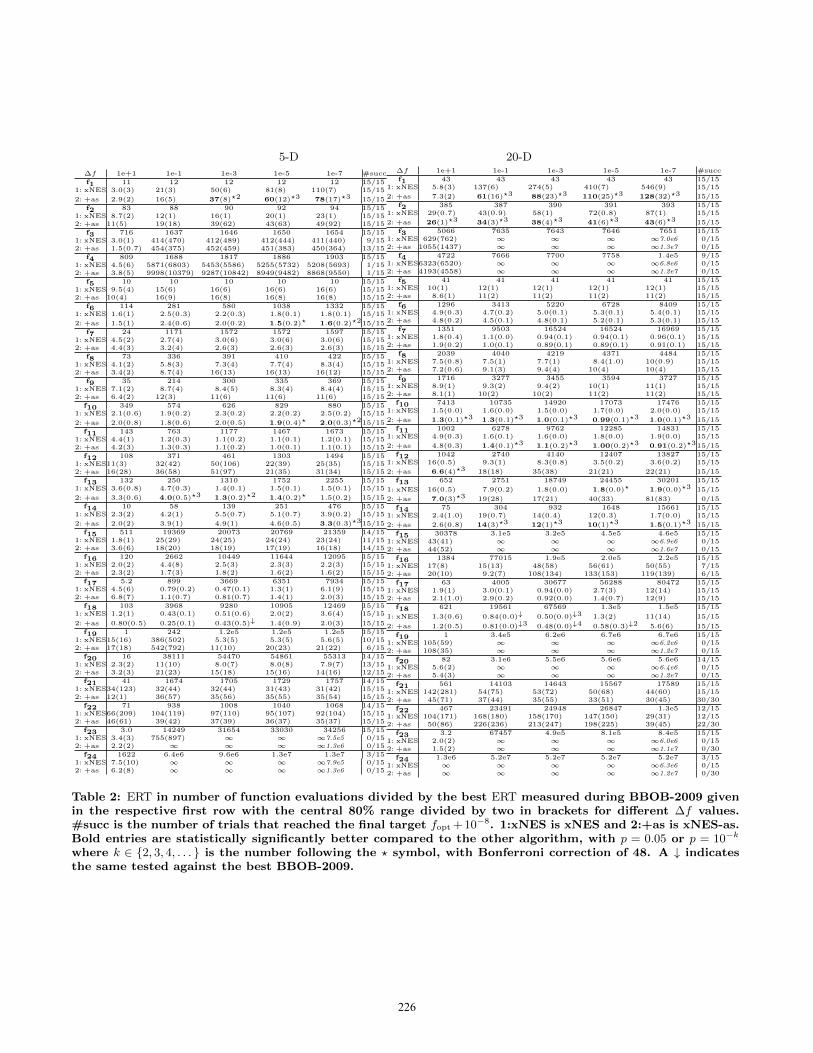
Table 2: ERT in number of function evaluations divided by the best ERT measured during BBOB-2009 givenin the respective first row with the central 80% range divided by two in brackets for different ∆f values.#succ is the number of trials that reached the final target fopt + 10−8. 1:xNES is xNES and 2:+as is xNES-as.Bold entries are statistically significantly better compared to the other algorithm, with p = 0.05 or p = 10−k
where k ∈ {2, 3, 4, . . . } is the number following the ? symbol, with Bonferroni correction of 48. A ↓ indicatesthe same tested against the best BBOB-2009.
226
5-D 20-Dnois
eles
sfu
nct
ions
0 1 2 3 4 5log10 of FEvals / DIM
0.0
0.5
1.0pro
port
ion o
f tr
ials
f1-24+1
-1
-4
-8
-5 -4 -3 -2 -1 0 1 2 3 4 5log10 of FEvals ratio
pro
port
ion
f1-24
+1: 24/24
-1: 23/22
-4: 22/22
-8: 22/22
0 1 2 3 4 5 6log10 of FEvals / DIM
0.0
0.5
1.0
pro
port
ion o
f tr
ials
f1-24+1
-1
-4
-8
-4 -3 -2 -1 0 1 2 3 4log10 of FEvals ratio
pro
port
ion
f1-24
+1: 23/23
-1: 17/17
-4: 17/17
-8: 17/16
nois
yfu
nct
ions
0 1 2 3 4 5log10 of FEvals / DIM
0.0
0.5
1.0
pro
port
ion o
f tr
ials
f101-130+1
-1
-4
-8
-5 -4 -3 -2 -1 0 1 2 3 4 5log10 of FEvals ratio
pro
port
ion
f101-130
+1: 30/30
-1: 28/28
-4: 20/20
-8: 19/19
0 1 2 3 4 5 6log10 of FEvals / DIM
0.0
0.5
1.0
pro
port
ion o
f tr
ials
f101-130+1
-1
-4
-8
-4 -3 -2 -1 0 1 2 3 4log10 of FEvals ratio
pro
port
ion
f101-130
+1: 24/24
-1: 14/14
-4: 11/12
-8: 10/11
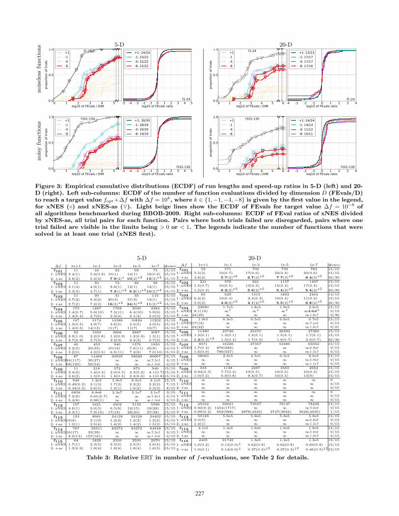
Figure 3: Empirical cumulative distributions (ECDF) of run lengths and speed-up ratios in 5-D (left) and 20-D (right). Left sub-columns: ECDF of the number of function evaluations divided by dimension D (FEvals/D)to reach a target value fopt+∆f with ∆f = 10k, where k ∈ {1,−1,−4,−8} is given by the first value in the legend,for xNES (◦) and xNES-as (O). Light beige lines show the ECDF of FEvals for target value ∆f = 10−8 ofall algorithms benchmarked during BBOB-2009. Right sub-columns: ECDF of FEval ratios of xNES dividedby xNES-as, all trial pairs for each function. Pairs where both trials failed are disregarded, pairs where onetrial failed are visible in the limits being > 0 or < 1. The legends indicate the number of functions that weresolved in at least one trial (xNES first).
5-D 20-D∆f 1e+1 1e-1 1e-3 1e-5 1e-7 #succ
f101 11 44 62 69 75 15/151: xNES 3.4(1) 5.4(0.9) 10(1) 14(1) 18(0.6) 15/15
2: +as 2.8(2) 5.2(2) 7.9(2)? 10(2)?3 13(3)?4 15/15
f102 11 50 72 86 99 15/151: xNES 3.1(4) 4.9(1) 8.8(1) 12(1) 14(1) 15/15
2: +as 3.3(3) 4.7(1) 7.3(1)?2 9.2(1)?310(2)?4 15/15
f103 11 30 31 35 115 15/151: xNES 3.7(2) 8.2(2) 20(3) 31(3) 13(1) 15/15
2: +as 2.7(2) 7.2(2) 16(3)?2 24(5)?2 11(2)?2 15/15
f104 173 1287 1768 2040 2284 15/151: xNES 1.4(0.7) 5.6(10) 7.3(11) 6.4(10) 5.9(9) 15/152: +as 1.4(0.4) 2.7(6) 2.3(4) 2.1(4) 2.0(3) 15/15
f105 167 5174 10388 10824 11202 15/151: xNES 1.3(0.5) 4.9(7) 3.6(5) 4.0(5) 4.0(5) 15/152: +as 1.4(0.5) 14(13) 11(7) 11(7) 10(7) 15/15
f106 92 1050 2666 2887 3087 15/151: xNES 2.9(1.0) 2.2(0.8) 1.2(0.9) 1.2(0.9) 1.3(1) 15/152: +as 2.7(0.8) 3.7(5) 2.2(3) 2.2(3) 2.7(3) 15/15
f107 40 453 940 1376 1850 15/151: xNES 3.2(3) 20(33) 10(16) 7.6(11) 45(8) 14/152: +as 3.2(5) 4.2(0.5) 6.9(11) 7.2(8) 7.0(10) 15/15
f108 87 14469 30935 58628 80667 15/151: xNES84(117) 36(27) ∞ ∞ ∞7.5e5 0/152: +as 69(120) 56(54) ∞ ∞ ∞1.3e6 0/15
f109 11 216 572 873 946 15/151: xNES 3.4(2) 1.4(0.3) 2.0(0.5) 2.3(0.2) 4.1(0.7)15/152: +as 3.6(2) 1.3(0.5) 1.8(0.5) 2.3(0.6) 4.1(0.8)15/15
f110 949 1.2e5 5.9e5 6.0e5 6.1e5 15/151: xNES 0.49(0.2) 2.1(3) 1.7(2) 2.2(2) 2.2(2) 7/152: +as 0.44(0.2) 3.6(5) 1.2(1) 1.6(2) 2.3(3) 8/15
f111 6856 8.8e6 2.3e7 3.1e7 3.1e7 3/151: xNES 7.2(9) 0.61(0.7) ∞ ∞ ∞7.8e5 0/152: +as 5.4(8) 0.96(1) ∞ ∞ ∞1.3e6 0/15
f112 107 3421 4502 5132 5596 15/151: xNES 4.6(1) 3.0(3) 6.5(8) 12(15) 18(28) 15/152: +as 2.3(1) 7.9(10) 17(18) 28(23) 37(38) 15/15
f113 133 8081 24128 24128 24402 15/151: xNES10(6) 2.1(3) 1.2(2) 1.2(2) 1.2(2) 15/152: +as 1.2(1) 2.5(4) 1.4(2) 1.4(2) 1.5(2) 15/15
f114 767 56311 83272 83272 84949 15/151: xNES10(17) 33(39) ∞ ∞ ∞7.5e5 0/152: +as 8.0(13) 157(161) ∞ ∞ ∞1.3e6 0/15
f115 64 1829 2550 2550 2970 15/151: xNES 1.7(1) 2.3(5) 2.5(5) 2.5(5) 2.6(4) 15/152: +as 1.3(0.9) 1.8(4) 1.8(4) 1.8(4) 1.6(3) 15/15
∆f 1e+1 1e-1 1e-3 1e-5 1e-7 #succ
f101 59 571 700 739 783 15/151: xNES 5.5(2) 10(0.7) 17(0.6) 24(0.4) 30(0.6) 15/15
2: +as 4.8(2) 5.7(2)?5 6.7(2)?5 7.7(3)?5 8.4(3)?5 30/30
f102 231 579 921 1157 1407 15/151: xNES 1.5(0.7) 10(0.5) 13(0.3) 15(0.2) 17(0.4) 15/15
2: +as 1.5(0.4) 6.2(2)?5 5.6(2)?5 5.4(2)?5 5.4(2)?5 30/30
f103 65 629 1313 1893 2464 14/151: xNES 6.2(2) 10(0.4) 9.4(0.3) 10(0.4) 11(0.3) 15/15
2: +as 5.0(2) 4.9(2)?5 4.1(2)?5 5.5(2)?5 6.8(2)?5 30/30
f104 23690 1.7e5 1.8e5 1.9e5 2.0e5 15/151: xNES 8.1(10) ∞? ∞? ∞? ∞8.0e6? 0/152: +as 24(29) ∞ ∞ ∞ ∞1.8e7 0/30
f105 1.9e5 6.3e5 6.5e5 6.6e5 6.7e5 15/151: xNES17(16) ∞ ∞ ∞ ∞7.4e6 0/152: +as 24(22) ∞ ∞ ∞ ∞1.6e7 0/21
f106 11480 23746 25470 26492 27360 15/151: xNES 1.3(0.1) 1.3(0.1) 1.3(0.1) 1.5(0.1) 1.7(0.1) 15/15
2: +as 1.2(0.2)?2 1.5(0.4) 1.7(0.9) 1.8(0.7) 2.0(0.7) 30/30
f107 8571 16226 27357 52486 65052 15/151: xNES 1.7(0.4) 879(889) ∞ ∞ ∞6.9e6 0/152: +as 1.6(0.9) 786(927) ∞ ∞ ∞1.5e7 0/15
f108 58063 2.0e5 4.5e5 6.3e5 9.0e5 15/151: xNES ∞ ∞ ∞ ∞ ∞5.9e6 0/152: +as ∞ ∞ ∞ ∞ ∞1.1e7 0/15
f109 333 1138 2287 3583 4952 15/151: xNES 0.94(0.3) 7.7(0.4) 10(0.5) 10(0.5) 10(0.3) 15/152: +as 1.0(0.2) 6.9(0.8) 9.4(0.7) 10(0.5) 13(8) 15/15
f110 ∞ ∞ ∞ ∞ ∞ 01: xNES ∞ ∞ ∞ ∞ ∞ 0/152: +as ∞ ∞ ∞ ∞ ∞ 0/15
f111 ∞ ∞ ∞ ∞ ∞ 01: xNES ∞ ∞ ∞ ∞ ∞ 0/152: +as ∞ ∞ ∞ ∞ ∞ 0/15
f112 25552 69621 73557 76137 78238 15/151: xNES 0.93(0.2) 1454(1717) ∞ ∞ ∞7.0e6 0/152: +as 0.99(0.2) 952(988) 3878(4223) 3747(3922) 3646(4035) 1/15
f113 50123 5.6e5 5.9e5 5.9e5 5.9e5 15/151: xNES 5.0(5) ∞ ∞ ∞ ∞6.8e6 0/152: +as 1.4(1) ∞ ∞ ∞ ∞1.5e7 0/15
f114 2.1e5 1.4e6 1.6e6 1.6e6 1.6e6 15/151: xNES ∞ ∞ ∞ ∞ ∞5.8e6 0/152: +as ∞ ∞ ∞ ∞ ∞1.0e7 0/15
f115 2405 91749 1.3e5 1.3e5 1.3e5 15/15
1: xNES 1.0(0.2) 0.14(0.0)↓ 0.62(0.8) 0.62(0.8) 0.69(0.8) 15/15
2: +as 1.0(0.1) 0.14(0.0)↓ 0.37(0.3)↓3 0.37(0.3)↓3 0.46(0.5)↓215/15
Table 3: Relative ERT in number of f-evaluations, see Table 2 for details.
227
5-D 20-D∆f 1e+1 1e-1 1e-3 1e-5 1e-7 #succ
f116 5730 22311 26868 30329 31661 15/151: xNES 0.62(1) 1.3(2) 1.2(1) 1.2(1) 1.2(1) 14/152: +as 1.4(2) 1.1(2) 1.3(1) 1.6(2) 1.8(2) 15/15
f117 26686 1.1e5 1.4e5 1.7e5 1.9e5 15/151: xNES 9.4(13) ∞ ∞ ∞ ∞7.6e5 0/152: +as 8.4(6) ∞ ∞ ∞ ∞1.3e6 0/15
f118 429 1555 1998 2430 2913 15/15
1: xNES 1.0(0.4) 0.52(0.1)↓4 0.73(0.1)↓2 1.0(0.2) 1.6(0.2)15/15
2: +as 1.00(0.4) 0.48(0.1)↓4 0.69(0.2)↓2 0.96(0.2) 1.1(0.2)15/15
f119 12 1136 10372 35296 49747 15/151: xNES 1.9(2) 0.66(0.2) 2.6(3) 1.5(1) 12(13) 9/152: +as 3.8(4) 6.3(13) 1.6(2) 2.3(3) 5.9(6) 15/15
f120 16 18698 72438 3.3e5 5.5e5 15/151: xNES 9.0(12) 43(39) ∞ ∞ ∞7.6e5 0/152: +as 51(18) 25(33) ∞ ∞ ∞1.3e6 0/15
f121 8.6 273 1583 3870 6195 15/151: xNES 2.7(3) 1.2(0.2) 1.3(0.5) 1.2(1) 1.7(2) 15/152: +as 2.6(2) 0.96(0.5) 1.6(0.8) 1.5(2) 2.3(3) 15/15
f122 10 9190 30087 53743 1.1e5 15/151: xNES 1.7(2) 6.4(4) 200(215) ∞ ∞8.5e5 0/152: +as 5.0(4) 8.9(8) 583(686) ∞ ∞1.3e6 0/15
f123 11 81505 3.4e5 6.7e5 2.2e6 15/151: xNES36(70) ∞ ∞ ∞ ∞7.5e5 0/152: +as 6.6(9) ∞ ∞ ∞ ∞1.3e6 0/15
f124 10 1040 20478 45337 95200 15/151: xNES 2.5(2) 3.8(10) 2.0(2) 19(20) 112(127) 1/152: +as 2.9(3) 2.0(0.7) 1.1(1) 36(40) 60(66) 1/15
f125 1 1 2.4e5 2.4e5 2.5e5 15/151: xNES 1.1 9476(14165) ∞ ∞ ∞7.6e5 0/152: +as 1.3(0.5) 7786(7916) ∞ ∞ ∞1.3e6 0/15
f126 1 1 ∞ ∞ ∞ 01: xNES 1.1 44499(50671) ∞ ∞ ∞ 0/152: +as 1.1(0.5) 41598(46392) ∞ ∞ ∞ 0/15
f127 1 1 3.4e5 3.9e5 4.0e5 15/151: xNES 1.1 3395(5420) 31(36) ∞ ∞7.4e5 0/152: +as 1.1(0.5) 3858(5345) ∞ ∞ ∞1.3e6 0/15
f128 111 7808 12447 17217 21162 15/151: xNES 7.1(2) 5.2(6) 3.3(4) 2.4(3) 2.0(2) 15/152: +as 22(67) 5.7(7) 3.6(4) 2.6(3) 2.1(2) 15/15
f129 64 59443 2.8e5 5.1e5 5.8e5 15/151: xNES38(34) 10(8) 11(13) ∞ ∞7.5e5 0/152: +as 17(16) 8.6(12) 14(16) ∞ ∞1.3e6 0/15
f130 55 3034 32823 33889 34528 10/151: xNES13(1) 25(25) 2.4(2) 2.3(2) 2.3(2) 15/152: +as 17(0.9) 28(48) 2.6(4) 2.5(4) 2.5(4) 15/15
∆f 1e+1 1e-1 1e-3 1e-5 1e-7 #succ
f116 5.0e5 8.9e5 1.0e6 1.1e6 1.1e6 15/151: xNES101(110) ∞ ∞ ∞ ∞7.1e6 0/152: +as 39(42) ∞ ∞ ∞ ∞1.6e7 0/15
f117 1.8e6 2.6e6 2.9e6 3.2e6 3.6e6 15/151: xNES ∞ ∞ ∞ ∞ ∞5.1e6 0/152: +as ∞ ∞ ∞ ∞ ∞8.1e6 0/30
f118 6908 17514 26342 30062 32659 15/151: xNES 1.0(0.0) 0.90(0.0) 1.1(0.1)1.5(0.1)1.8(0.0) 15/15
2: +as 0.94(0.1)?3 0.80(0.1)?31.1(0.1)1.7(0.7)2.1(0.7) 15/15
f119 2771 35930 4.1e5 1.4e6 1.9e6 15/15
1: xNES 0.54(0.3)↓2 2741(2972) ∞ ∞ ∞6.7e6 0/15
2: +as 0.53(0.4)↓ 851(771) ∞ ∞ ∞1.4e7 0/13
f120 36040 2.8e5 1.6e6 6.7e6 1.4e7 13/151: xNES 14(23) ∞ ∞ ∞ ∞6.0e6 0/152: +as 6.9(7) ∞ ∞ ∞ ∞1.1e7 0/15
f121 249 1426 9304 34434 57404 15/151: xNES 0.74(0.2) 6.7(0.4) 2.9(0.2)1.3(0.1)1.1(0.1) 15/152: +as 0.81(0.3) 6.3(0.5) 2.9(0.2)1.7(0.6)1.7(1) 15/15
f122 692 1.4e5 7.9e5 2.0e6 5.8e6 15/151: xNES 0.91(0.8) ∞ ∞ ∞ ∞6.2e6 0/152: +as 0.81(0.9) ∞ ∞ ∞ ∞1.2e7 0/13
f123 1063 1.5e6 5.3e6 2.7e7 1.6e8 01: xNES 9.0(9) ∞ ∞ ∞ ∞6.1e6 0/152: +as 11(14) ∞ ∞ ∞ ∞1.1e7 0/15
f124 192 40840 1.3e5 3.9e5 8.0e5 15/151: xNES 0.63(0.3) 0.58(0.1) 6.4(7) ∞ ∞6.9e6 0/152: +as 0.84(0.3) 0.59(0.1) 4.0(3) ∞ ∞1.8e7 0/15
f125 1 1 2.5e7 8.0e7 8.1e7 4/151: xNES 1.5(1) ∞ ∞ ∞ ∞6.1e6 0/302: +as 1.7(1) ∞ ∞ ∞ ∞1.1e7 0/15
f126 1 1 ∞ ∞ ∞ 01: xNES 1.2(0.5) ∞ ∞ ∞ ∞ 0/302: +as 1.4(1) ∞ ∞ ∞ ∞ 0/15
f127 1 1 4.4e6 7.3e6 7.4e6 15/151: xNES 1.4(1) ∞ ∞ ∞ ∞6.1e6 0/302: +as 1.5(0.5) ∞ ∞ ∞ ∞1.1e7 0/15
f128 1.4e5 1.7e7 1.7e7 1.7e7 1.7e7 9/151: xNES 28(32) 1.2(1) 2.0(2) 3.4(4) 3.4(4) 3/302: +as 19(23) 0.78(0.9) 1.0(1) 1.0(1.0)1.3(1) 6/15
f129 7.8e6 4.2e7 4.2e7 4.2e7 4.2e7 5/151: xNES ∞ ∞ ∞ ∞ ∞6.0e6 0/302: +as ∞ ∞ ∞ ∞ ∞1.1e7 0/15
f130 4904 2.5e5 2.5e5 2.6e5 2.6e5 7/151: xNES 14(20) 4.9(6) 4.9(5) 4.9(5) 4.9(5) 29/302: +as 15(23) 5.4(9) 5.4(9) 5.4(9) 5.4(9) 15/15
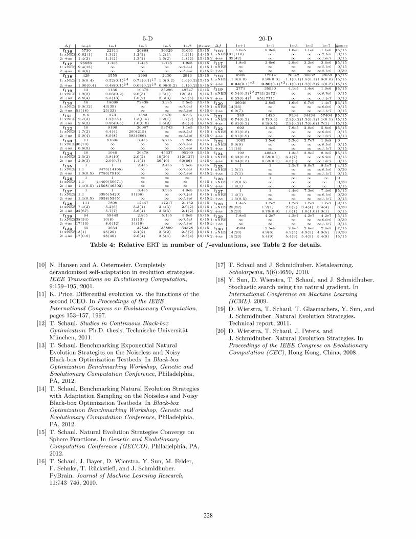
Table 4: Relative ERT in number of f-evaluations, see Table 2 for details.
[10] N. Hansen and A. Ostermeier. Completelyderandomized self-adaptation in evolution strategies.IEEE Transactions on Evolutionary Computation,9:159–195, 2001.
[11] K. Price. Differential evolution vs. the functions of thesecond ICEO. In Proceedings of the IEEEInternational Congress on Evolutionary Computation,pages 153–157, 1997.
[12] T. Schaul. Studies in Continuous Black-boxOptimization. Ph.D. thesis, Technische UniversitatMunchen, 2011.
[13] T. Schaul. Benchmarking Exponential NaturalEvolution Strategies on the Noiseless and NoisyBlack-box Optimization Testbeds. In Black-boxOptimization Benchmarking Workshop, Genetic andEvolutionary Computation Conference, Philadelphia,PA, 2012.
[14] T. Schaul. Benchmarking Natural Evolution Strategieswith Adaptation Sampling on the Noiseless and NoisyBlack-box Optimization Testbeds. In Black-boxOptimization Benchmarking Workshop, Genetic andEvolutionary Computation Conference, Philadelphia,PA, 2012.
[15] T. Schaul. Natural Evolution Strategies Converge onSphere Functions. In Genetic and EvolutionaryComputation Conference (GECCO), Philadelphia, PA,2012.
[16] T. Schaul, J. Bayer, D. Wierstra, Y. Sun, M. Felder,F. Sehnke, T. Ruckstieß, and J. Schmidhuber.PyBrain. Journal of Machine Learning Research,11:743–746, 2010.
[17] T. Schaul and J. Schmidhuber. Metalearning.Scholarpedia, 5(6):4650, 2010.
[18] Y. Sun, D. Wierstra, T. Schaul, and J. Schmidhuber.Stochastic search using the natural gradient. InInternational Conference on Machine Learning(ICML), 2009.
[19] D. Wierstra, T. Schaul, T. Glasmachers, Y. Sun, andJ. Schmidhuber. Natural Evolution Strategies.Technical report, 2011.
[20] D. Wierstra, T. Schaul, J. Peters, andJ. Schmidhuber. Natural Evolution Strategies. InProceedings of the IEEE Congress on EvolutionaryComputation (CEC), Hong Kong, China, 2008.
228