1

Investigating the impact of reemerging sea surface

temperature anomalies on the winter atmospheric

circulation over the North Atlantic

Christophe Cassou1, 2, Clara Deser2 and Michael A. Alexander3

(1) CNRS-CERFACS, Toulouse, France

(2) National Center for Atmospheric Research, Boulder, USA

(3) NOAA-CIRES, Climate Diagnostics Center, Boulder, USA

Submitted to Journal of Climate 29 March 2006

Corresponding Author: Christophe Cassou

CERFACS-CNRS 42, Avenue G. Coriolis

31057 TOULOUSE Cedex 01, France Tel: +33 561 19 30 49

Email: cassou@cerfacs.fr

2

Abstract In the extratropics, thermal anomalies stored in the deep winter oceanic mixed layer persist at depth through summer, insulated from direct air-sea interaction, and become re-entrained into the seasonal deepening mixed layer during the following winter. This so-called “reemergence mechanism” contributes to the observed winter-to-winter persistence of sea surface temperature anomalies. This study investigates the impact of oceanic reemergence upon the atmosphere in the North Atlantic using a simplified coupled model (atmospheric general circulation model coupled to a mixed layer ocean model and a thermodynamical ice model). Such a model configuration takes into account vertical oceanic processes such as entrainment, and provides a realistic physical representation of ocean-atmosphere-ice interaction at the interface.

An estimate of the extratropical oceanic thermal anomalies created by the atmosphere in late-winter and subsequently stored within the highly stratified summer thermocline is obtained from a long control simulation of the coupled model. These thermal anomalies strongly project onto the upper branches of the so-called North Atlantic tripole pattern forced by the previous winters North Atlantic Oscillation (NAO). To investigate the impact of these subsurface thermal anomalies upon the following winter’s atmospheric circulation, we incorporate them into the oceanic initial conditions of a 60-member ensemble of integrations of the coupled model beginning on August 1st and extending for 1 year. We show that the reemergence of the extratropical SST anomaly tripole occurs in November/December and lasts through the following spring. The reemerging SST anomalies have a significant impact upon the model atmosphere, favoring the same phase of the NAO as that which created them the previous winter. The atmospheric model response represents a 15-20% positive feedback and thus weakly enhances the winter-to-winter persistence of the NAO. The large-scale atmospheric response includes a modification of the transient eddies associated with changes in the occurrence of intrinsic weather regimes whose temporal integration yields the mean winter NAO response. Eddy-mean flow interactions contribute to the large-scale persistent atmospheric response to the reemerging SST anomalies, and are speculated to control its timing.

1. Introduction

It is well established that the North Atlantic atmosphere is primarily governed by internal chaotic behavior, therefore considerably reducing its low frequency potential predictability (Rodwell 2003). A series of observational, theoretical and modeling studies have suggested though that the North Atlantic atmosphere is slightly modulated by a multitude of very weakly coupled processes and/or external forcings involving all the climate components over a wide range of interacting timescales (see Hurrell et al 2003 for a review). These processes or forcings could explain why the main variability mode of the North Atlantic atmosphere, known as the North Atlantic Oscillation (NAO), exhibits a temporal spectrum that is slightly inconsistent with a first order autoregressive process, which is traditionally used to describe pure climate noise (Feldstein 2000). In

3

particular, these processes could be at the origin of “shoulders” in the NAO spectrum or low frequency persistence explaining its reddish shape (Greatbatch 2000), even if the latter is still controversial (Wunsch 1999, Stephenson et al 2000).

At decadal or longer timescales, the North Atlantic Ocean, as a heat carrier and a

heat reservoir, is found to be weakly coupled to the North Atlantic atmosphere via the fluctuations of the oceanic meridional overturning circulation (Delworth 1996, Timmermann et al 1998, Dong and Sutton 2001) or the Atlantic Multidecadal Oscillation (AMO, Sutton and Hodson 2005). In the interannual band, remote oceanic forcings like El Niño Southern Oscillation (ENSO) have been found to contribute to the 4-5yr spectral bump (Cassou and Terray 2001) of the NAO and tropical-extratropical connections through forced Rossby waves originating from the tropical Atlantic basin also operate in the 7-10yr window (Venske et al 1999, Sutton et al 2001, Terray and Cassou 2002, Drévillon et al 2003). Given the large environmental and socio-economical impacts of the NAO over Europe and eastern North America (Hurrell 1995), it is therefore of interest to investigate the nature of the NAO temporal behavior. Advancing understanding of its underlying mechanisms is a key challenge to improve seasonal-to-interannual predictive skill. In the present study, we focus on understanding the considerable degree of year-to-year correlation of the NAO especially during the winter season.

The NAO can be viewed as a stationary, equivalent barotropic meridional mass balance between the Icelandic low and the Azores high. It can also be described as a self-maintaining meridional shift in the eddy-driven North Atlantic jet (see Hurrell et al 2003 for a review). A strong coherence is found between the dominant patterns of monthly to seasonal sea surface temperature (SST) anomalies and the spatio-temporal structure of the NAO. The association is strongest in winter when atmospheric internal perturbations grow to their largest amplitude and locally imprint their signature on the well-mixed upper-ocean layer. The prime direction of the forcing is undoubtedly from the atmosphere to the ocean as shown for instance by Deser and Timlin (1997) which puts the atmospheric lead at 2-3 weeks. Anomalous turbulent heat fluxes, buoyancy-driven entrainment and Ekman advection are the main processes whereby the NAO then forces an anomalous SST tripole pattern in the North Atlantic (Cayan 1992, Seager et al 2000). The typical e-folding timescale of its surface signature is on the order of 3-5 months (see a review in Frankignoul 1985) and in such a scenario, the low frequency oceanic anomalies are considered as the passive temporal integration of the atmosphere stochastic forcing (Frankignoul and Hasselmann 1977, hereafter FH77). Recent studies have provided evidence that the FH77 paradigm may be however too simple to correctly reproduce the North Atlantic ocean-atmosphere interaction. In particular, it does not take into account the local air-sea adjustment which leads to a reduction of the thermal damping exerted by the ocean on the atmosphere as the former responds to variations in the surface heat fluxes. This process is expected to enhance the persistence of the atmospheric fluctuations in the monthly to interannual spectral band (Barsugli and Battisti 1998). In addition, it underestimates the role of the vigorous wintertime transient atmospheric eddies whose associated feedback appear to play a significant role in both modulating and maintaining the wintertime ocean-atmosphere

4

anomalies (Peng and Whitaker 1999). Finally, because the FH77 conceptual model neglects the seasonal variations of oceanic processes, in particular the strong seasonal cycle of the mixed layer depth, Deser et al (2003) and de Coëtlogon and Frankignoul (2003) show that it misses the so-called reemergence mechanism (Alexander and Deser 1995) that strongly contributes to shaping the year-to-year recurrence of the wintertime North Atlantic SST tripole (Watanabe and Kimoto 2000, Timlin et al 2002). During winter, vigorous air-sea energy exchange creates temperature anomalies that extend down to the base of the deep oceanic mixed layer. When the latter rapidly shoals in spring in response to increasing solar radiation and weakening stirring due to the seasonal slackening of surface winds and surface turbulent fluxes, the winter thermal oceanic anomalies become insulated from the surface and the damping effect of negative heat flux feedbacks characteristic of the extratropics (Frankignoul and Kestenare 2002). These anomalies persist throughout summer beneath the very shallow summer mixed layer within the stably stratified seasonal thermocline. Their sequestration ends in the following fall or early winter when the mixed layer deepens again due to the seasonal intensification of the extratropical atmospheric circulation. They become re-entrained at the base of the newly eroding mixed layer and modify its heat balance with the surface. This re-entrainment thus leads to reemergence of the previous winter’s SST anomalies. Oceanic reemergence occurs basin-wide both in the Pacific (Alexander et al 1999) and the Atlantic (de Coëtlogon and Frankignoul 2003). Its timing and intensity are function of the depth of the winter mixed layer and the strength of the wintertime atmospheric forcing. In the Atlantic, Alexander and Penland (1996) and Alexander et al (2000) indicate that entrainment significantly contributes to the growth of large scale SST anomalies in fall and may explain very well the year-to-year persistence of the wintertime SST tripole. If the reemerging ocean forcing is exported to the upper atmosphere and sufficiently efficient to modify the large-scale atmospheric dynamics, the latter could explain some reddening in the energy concentration of the observed NAO spectrum in the interannual band. In this study, we will investigate to what extent the reemergence process accounts for the observed persistence of the winter NAO whose origin remains obscure, and by which processes the ocean memory is possibly passed to the overlying atmosphere. While addressing these questions, we have to keep in mind that the dominant source of NAO variability is internal atmospheric dynamics. Thus, Junge and Haine (2001) suggest that even if reemergence does play a role, contemporaneous heat flux anomalies are much more effective at generating wintertime SST anomalies. For the atmosphere, Kushnir et al (2002) state that external forcings all together could explain at most 20-25% of the interannual variance of the North Atlantic atmosphere. Nevertheless, as pointed out in the Kushnir et al. review, much can be gained in seasonal-to-interannual prediction from better resolving and understanding all the weakly coupled processes involved in North Atlantic climate, which could have a significant impact under particular conditions. Isolating and quantifying the role of reemergence in the winter-to-winter NAO persistence is difficult from both observations and fully coupled models where the

5

simultaneous and dominant forcing of the atmosphere on the underlying ocean masks a potential response. In this study, we use a simplified coupled AGCM-ocean mixed layer model that includes a thermodynamic sea-ice component. Such a coupled system allows for reemergence by incorporating the dominant vertical oceanic processes. We will analyze an ensemble of experiments where we impose thermal heating anomalies below the thin summer mixed layer and let them be re-entrained back to the surface in the following winter. Such a coupled model accounts for local air-sea interaction as well as air-sea-ice exchanges that have been shown to play a significant role in shaping the North Atlantic atmospheric variability. By using such a system, we also avoid the difficult task of dealing with model drift maintaining a reasonable mean ocean climate via a flux correction term that mainly compensates for the absence of oceanic heat transport, and for model biases to a lower extent. On the other hand, we neglect the non-locality of the reemergence due to oceanic advection that may add some persistence to the wintertime SST anomalies and associated atmospheric circulation as suggested by de Coëtlogon and Frankignoul (2003). The paper is organized as follows. The atmosphere, ocean and ice components of the coupled model, the method of coupling and the model performance are described in section 2. The experimental setup chosen to isolate, quantify, and understand the impact of the reemergence on the North Atlantic atmosphere is presented in section 3. The simulated atmospheric response to imposed reemerging thermal oceanic anomalies is examined in section 4. Processes involved in the atmospheric response, their timing and their amplitude, are also explored. The results are summarized and further discussed in section 5. 2. Coupled model description and performance

a. Model components The coupled model used in this study has four components. The model

atmosphere is the second version of the Community Atmosphere Model (CAM2.1), primarily developed at the National Center for Atmospheric Research (NCAR). The AGCM dynamics is based upon an eulerian spectral scheme solved on a Gaussian grid of about 2.8o x 2.8o latitude-longitude corresponding to a triangular horizontal truncation at 42 wave numbers. The vertical resolution is discretized over 26 levels using a progressive vertical hybrid coordinate. The reader is invited to refer to Kiehl and Gent (2004) for a detailed description of the model physics package and for its performance. The land surface and the sea-ice components are the Community Land Model (CLM2, Oleson et al 2004) and the Community Sea-Ice Model (CSIM, Briegleb et al 2004), respectively. The dynamical core of the latter has been turned off in the present case. The ocean component consists of single independent column models with explicit mixed layer physics and no horizontal advection. Land, sea-ice and ocean models are aligned with the CAM grid. Coupling between the ocean and the other components occurs daily, while the atmosphere, ice and land modules exchange flux and mass quantities at the CAM time step.

6

The ocean mixed layer model (MLM) is based on Gaspar (1988)’s formulation as implemented by Alexander and Deser (1995). In the present study, we use a modified version of that used in Alexander et al (2000) where we include additional layers, extend the ocean bottom to 1500m (instead of 1000m) and implement coupling between the thermodynamical sea-ice component of CSIM and the MLM surface layer. Each ocean point has 36 vertical levels with 15 layers in the upper 100m and a realistic bathymetry. Very shallow areas (< 40 m) are treated as a fixed 50m-depth slab ocean. Others have a varying mixed layer depth (MLD) computed as a prognostic variable based on turbulent kinetic energy parameterization when deepening, or as a diagnostic quantity based on the balance between wind stirring and surface buoyancy forcing when shoaling. Surface heat flux (Qcor) and salinity flux (Scor) correction terms are applied to account for all the missing physics in the ocean such as heat and salinity transport by the mean currents, diffusion etc as well as errors in the atmospheric surface fluxes to a lower extent. Heat is mainly added in the winter hemisphere oceans while it is extracted year-round in the deep tropics, especially in the Pacific and Atlantic (Fig.1ab). The latter compensates for missing horizontal ocean advection along the equatorial cold tongues and their associated upwelling. The former compensates for the missing meridional advection along the Gulf Stream and its North Atlantic extension, as well as along the Kuroshio Current in the Pacific (Fig.1a). In JJA and in the southern hemisphere, winter Qcor brings heat along the storm track into the mixed layer, which is fed in nature by intrusions of warm intermediate waters that are not simulated in MLM (Fig. 1b). The reader is invited to visit the following web address (http://www.cgd.ucar.edu/cas/cdeser/REMsupfig.html) to obtain a complete description of the model, including equations, and for further details on the computational methods and correction terms. b. The coupled model mean state We performed a 150-yr coupled integration hereafter referred to as CTL. The model reproduces rather well the SST mean state and differences between CTL and observed SST climatologies are weak as shown in Fig. 1cd. Year-round tropical and midlatitude winter SSTs are very well simulated (within +/-0.3oC bias). The largest errors occur in summer in the extratropical oceans which are overly too warm due to shallower-than-observed MLD especially in the southern hemisphere (around +1.2oC, Fig. 1c). A moderate warming occurs as well in boreal winter in the Labrador Sea along the Labrador Current (~+1oC, Fig. 1c) and is attributed to the crude representation of ice and salinity related processes (dynamics in particular) that control a large part of the ocean vertical profiles in these regions. Despite a slight underestimation of the ice extent in summer (Fig.1f) leading to local SST biases (Fig.1d), the simulated sea-ice matches very well the estimated observed extent especially in winter (Fig. 1e). Marginal errors are found along the Greenland Sea ice tongue that is slightly too broad and in the Labrador Sea where the winter sea-ice does not penetrate enough southeastward, consistently with the warmer SST. In the southern hemisphere, biases are minor for sea-ice (not shown). Note here that the implementation of the fresh water/salinity flux exchanges between the ocean and ice model components appeared crucial in both controlling the wintertime sea-ice spatial growth, mostly through

7

brine rejection, and initiating the summertime melting. The reader is invited to visit the above-mentioned web page for further detail. As found in observations (see, de Boyer Montegut et al 2004 for instance), the deepest MLD occurs in the winter hemisphere in CTL (Fig. 1gh). In the northern hemisphere, maxima follow the vigorous storm tracks both in the North Pacific and in the North Atlantic with correctly simulated values between 150-200 meters (Fig. 1g). Greater depths are found between Greenland and Great Britain as well as in the Labrador and Norwegian Sea. In CTL, even if some grid points around Iceland and Spitzberg reach 600-700 meters, the observed plunging of the mixed layer associated with deep water formation is however clearly underestimated with mean simulated values around 250m in the subarctic seas. Such a weak magnitude is very common for this type of model and resolution and the reader is invited to refer to as Alexander et al (2000) for a list of factors that may contribute to such a model behavior.

Note finally that there is no significant drift in the coupled model over open water in MLD, temperature and salinity. However a clear trend in salinity is found under sea-ice points. 3. Experimental setup The spatio-temporal characteristics of the oceanic reemerging pattern is now investigated in CTL from lead-lag maximum covariance analysis (e.g., von Storch and Zwiers 1999) based on singular value decomposition (SVD) between July-September (JAS) subsurface temperature anomalies from 40m to 400m depth in the North Atlantic (north of 25oN) and SLP at various lead times over a North Atlantic-European domain (20o-85oN/90oW-30oE). In the SVD analysis, the ocean temperature is treated as a vector-valued field and the covariance matrix can be viewed as a collection of submatrices, which contain the covariances between SLP and levels of ocean temperature jointly at the same grid point. Table 1 gives SVD statistics for the leading SVD mode as a function of lead time from November-January (SLP leading ocean temperature by 8 months) to JAS (atmosphere and ocean in phase). The greatest covariances are found in CTL between the summer subsurface ocean and the previous winter atmosphere indicative of the atmosphere forcing the ocean, while contemporaneous or quasi-contemporaneous (from MJJ) ocean-atmosphere links are weak and not significant. The strongest and robust link is established between the February-April (FMA) NAO (Fig. 2a), and the JAS subsurface thermal signature of North Atlantic tripole (Fig. 2b). Principal component (PC) time series of the two SVD modes are dominated by interannual-to-decadal fluctuations and are significantly correlated as portrayed in Fig. 2c. Our results from a coupled model are consistent with Timlin et al (2002) and de Coëtlogon and Frankignoul (2003) findings from observations. The role of the late winter atmosphere in shaping the following summer subsurface ocean anomalous pattern is further confirmed in Fig. 3 for CTL. A temperature index computed as the averaged anomalies over the ocean first 30 meters in the Labrador Sea [50o-60oN, 60oW-30oW] in March, corresponding to the location and timing of the maximum ocean anomalous pattern extracted from SVD (Fig. 2b), is

8

correlated to temperature as a function of month and depth over the same domain. While correlation values near the surface (0-30 m) decline from April until the following September, those at depth (50-100 m) exhibit almost no attenuation, corroborating the SVD results. A portion of the signal indicated by correlation values greater than 0.65 rebounds to the surface in October and November in phase with the seasonal deepening of the mixed layer (thick curve). Thereafter, the correlations decay rapidly along the entire mixed column, similar to observations although less pronounced (Alexander et al 1999). Such a decrease is consistent with the effect of entrainment, which mixes the existing heat content anomalies with thermal anomalies newly created by the wintertime atmospheric anomalies. In CTL, the rapid loss of memory is amplified as the North Atlantic MLD is underestimated and because the simulated NAO is characterized by a too strong quasi-biennal component (not shown) thus considerably reducing its winter-to-winter persistence compared to observations. The impact of the reemerging thermal anomalies on the atmosphere is consequently hard to extract from CTL only; however Fig. 3 shows that the reemergence indeed occurs in the coupled model but mostly as a “stand alone” oceanic process. To isolate and determine the influence of the reemergence on the atmosphere, two 60-member ensembles of coupled experiments, hereafter REM+ and REM-, are performed based on the FMA/JAS atmosphere/ocean SVD results. All members of each ensemble are integrated for a year starting Aug. 1st with the same perturbed initial oceanic conditions but different initial atmospheric states. The common ocean conditions correspond to the 3-dimensional thermal anomalies given by the SVD mode that are added in REM+ (subtracted in REM-) to the 150-yr averaged Aug. 1st ocean conditions computed from CTL. The atmospheric conditions are taken randomly among the 150 Aug. 1st atmospheric conditions from CTL. The spatial shape and the intensity of the imposed ocean perturbations are obtained by multiplying the 3-dimensional SVD oceanic mode by the maximum of the SLP PC time series (3.1: see Fig. 2c), to preserve linear relations between the variables. As illustrated in Fig.4, maximum amplitudes of the REM+ perturbations are found in the western part of the North Atlantic basin and reach 1.2oC in the Labrador Sea (Fig. 4a) and 0.8oC off the eastern US coast (Fig. 4b). Anomalies are mostly confined between 40m and 125m depth, below the summer mixed layer of CTL (thick solid curve) but within the winter mixed layer (thick dashed curve).

Note that the amplitudes of the oceanic perturbations are moderate and their spatial pattern slightly northward shifted compared to observational estimates (de Coëtlogon and Frankignoul 2003). We have chosen to apply a realistic NAO forced signal (but the strongest extracted from CTL) so that we can compare the amplitude of the model response to observations with more confidence. Also, we use a simulated pattern from CTL as opposed to one directly derived from observations for the forcing so that it is consistent with the coupled model dynamics and physics and is thus expected to maximize the model sensitivity to the reemergence process. As suggested by numerous studies (see Kushnir et al 2002 for a review), a spatial match between surface ocean anomalies and atmospheric entities (position of the jet, intensity of the storm track etc.) appears to be a necessary condition to obtain a significant signal in the midlatitude atmosphere in response to midlatitude SST anomalies. In the following, we mostly

9

examine the linear portion of the coupled model response by taking the ensemble-mean difference between REM+ and REM-, hereafter referred to as REM. 4. Results

a. Temporal evolution of the simulated ocean anomalies

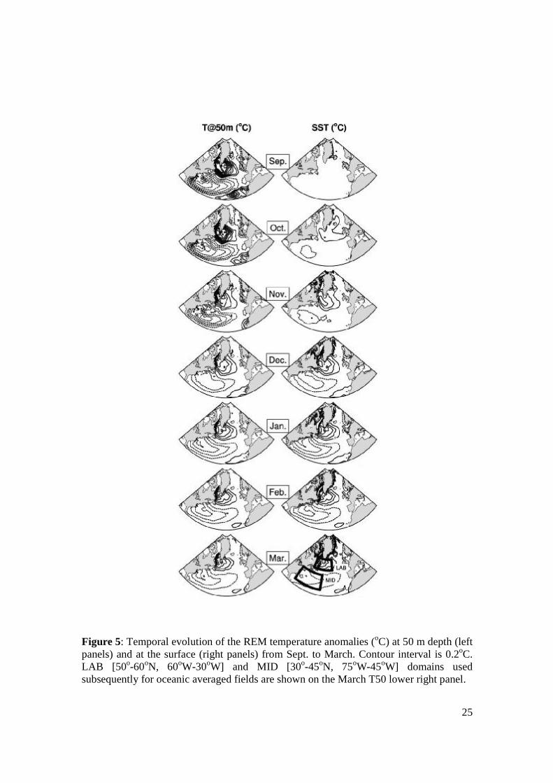
The monthly evolution of the REM temperature anomalies at 50 m depth (hereafter T50, left panels) and at the surface (right panels) are contrasted in Fig. 5. The midlatitude ocean pattern imposed in the MLM initial conditions is well preserved at the subsurface in September while there is no surface signature yet. Some weak SST signals show up in October and are then clearly amplified in November for the northernmost part of the basin, and in December for the midlatitudes. The latter mimic the subsurface temperature anomalies, which are, by contrast, concomitantly damped between October and November in the Labrador Sea, and between November and December for regions off the US coast. From December onward, surface and subsurface patterns match perfectly and both exhibit some intensification in January before a gradual slackening.

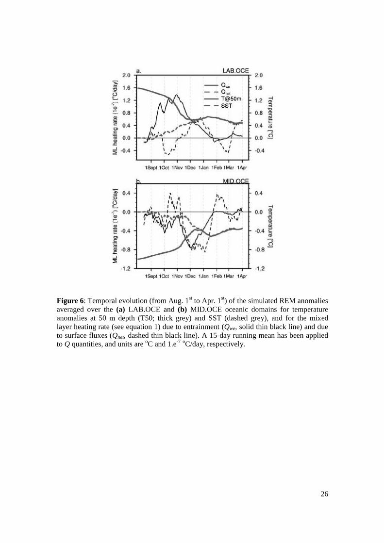
Further detail on the temporal evolution of the simulated ocean anomalies is given in Fig. 6, which separately examines, on a daily basis, the vertical entrainment (Qwe) contribution and the surface heat flux (Qnet) contribution in the mixed layer temperature change (see the above-mentioned web page for MLM equations). Over the Labrador Sea (LAB.OCE box defined in Fig.5), the heating rate due to entrainment rapidly increases and significantly contributes to the mixed layer warming from mid-September to mid-November (Fig. 6a). It is particularly active in late October where the temperature anomalies imposed below the seasonal thermocline in the sensitivity experiments are brought back within the deepening mixed layer. Such a timing is consistent with the mean seasonal evolution of the MLD presented previously in Fig. 3 for CTL and leads to a significant drop of the T anomalies at 50m depth (hereafter T50). SST and T50 are identical when MLD exceeds 50m, i.e. around mid-December, while the Qwe contribution progressively diminishes. From January onward, the SST changes are mostly controlled by the Qnet term. Note that Qnet tends to counteract the entrainment forcing in early fall, reducing the rate of SST warming, while it amplifies the SST anomalies from December onward, as also noted previously in Fig. 5. Similar results are found for the mid-Atlantic region (MID.OCE) with a one month delay (Fig. 6b). Maximum cooling due to re-entrainment at the base of the mixed layer in response to the presence of negative thermal anomalies occurs in late November in phase with the seasonal deepening of the mixed layer for that region (not shown). Negative SST anomalies develop rapidly at the beginning of December, while T50 anomalies are damped. Both later coincide at the end of December, when MLD is greater than 50 m, and are further reinforced by the Qnet contribution. Note that the Qnet timing is similar at mid and high latitudes whereas all oceanic quantities are delayed by one month. February contrasts with the other winter months as Qnet damps the SST anomalies in both domains before amplifying them from March onward.

10

Collectively, the results suggest that the REM SST anomalies developing in the sensitivity experiments at the beginning of winter are forced by the reemergence processes. In particular, we have shown that the Qwe contribution dominates the Qnet effect in their genesis. The model configuration used in this study thus appears to be a relevant tool to further isolate and investigate the role of reemergence in accounting for the winter-to-winter persistence of the NAO.

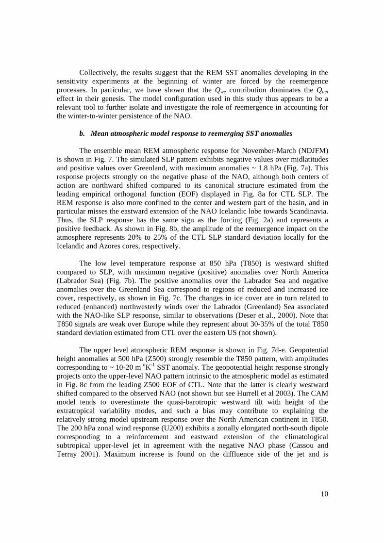
b. Mean atmospheric model response to reemerging SST anomalies The ensemble mean REM atmospheric response for November-March (NDJFM)

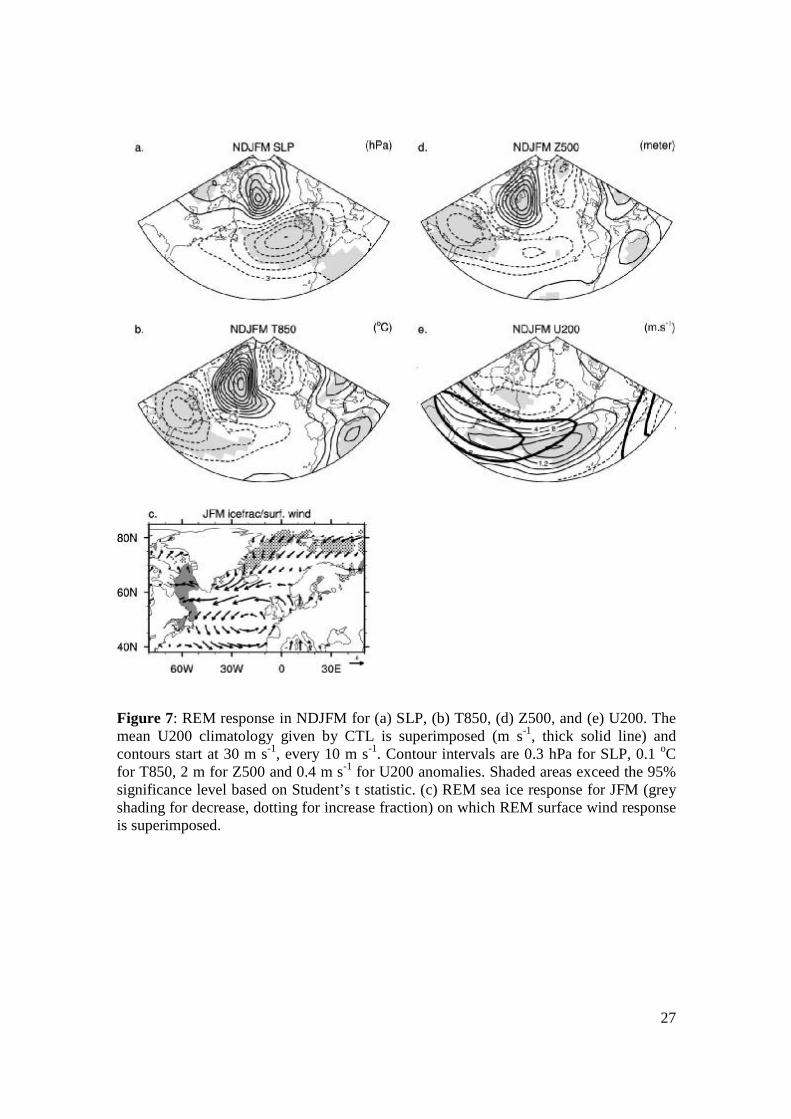
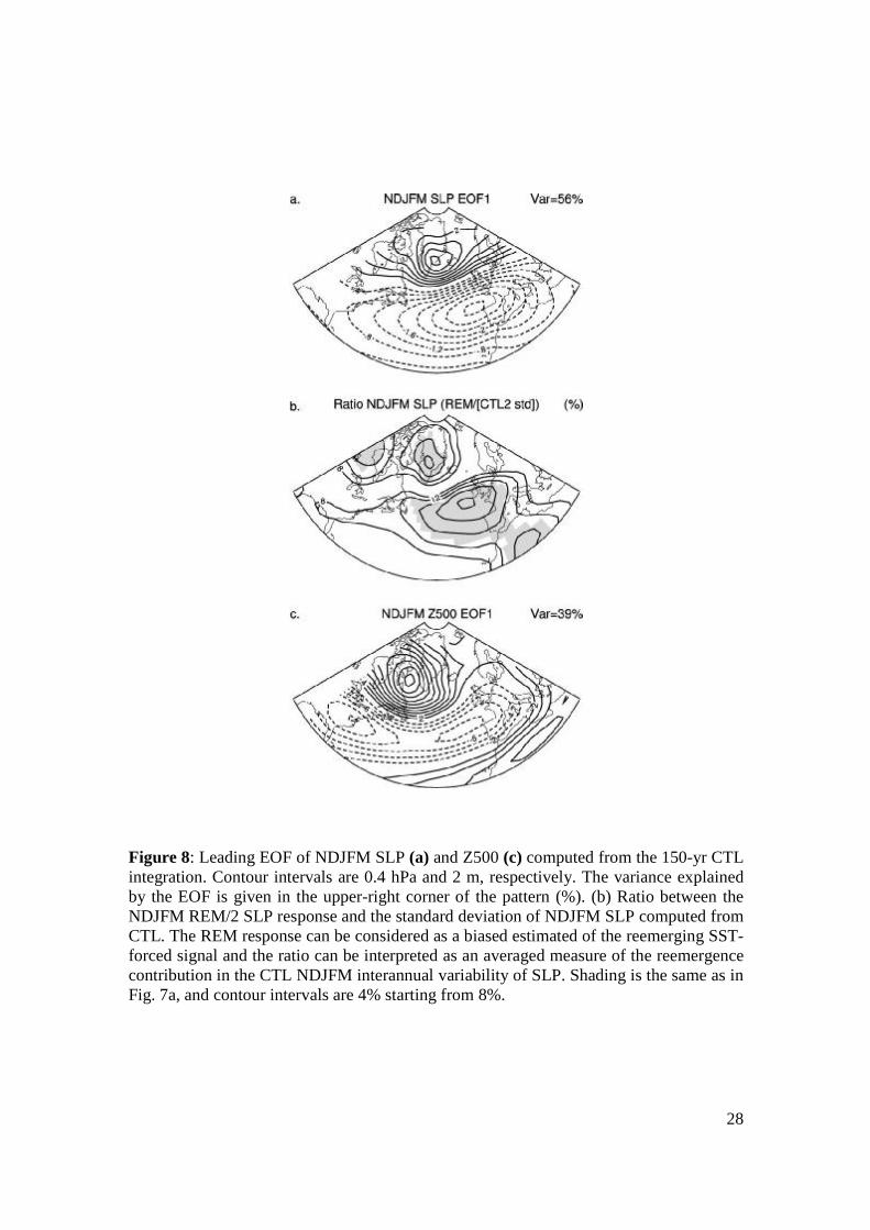
is shown in Fig. 7. The simulated SLP pattern exhibits negative values over midlatitudes and positive values over Greenland, with maximum anomalies ~ 1.8 hPa (Fig. 7a). This response projects strongly on the negative phase of the NAO, although both centers of action are northward shifted compared to its canonical structure estimated from the leading empirical orthogonal function (EOF) displayed in Fig. 8a for CTL SLP. The REM response is also more confined to the center and western part of the basin, and in particular misses the eastward extension of the NAO Icelandic lobe towards Scandinavia. Thus, the SLP response has the same sign as the forcing (Fig. 2a) and represents a positive feedback. As shown in Fig. 8b, the amplitude of the reemergence impact on the atmosphere represents 20% to 25% of the CTL SLP standard deviation locally for the Icelandic and Azores cores, respectively.

The low level temperature response at 850 hPa (T850) is westward shifted compared to SLP, with maximum negative (positive) anomalies over North America (Labrador Sea) (Fig. 7b). The positive anomalies over the Labrador Sea and negative anomalies over the Greenland Sea correspond to regions of reduced and increased ice cover, respectively, as shown in Fig. 7c. The changes in ice cover are in turn related to reduced (enhanced) northwesterly winds over the Labrador (Greenland) Sea associated with the NAO-like SLP response, similar to observations (Deser et al., 2000). Note that T850 signals are weak over Europe while they represent about 30-35% of the total T850 standard deviation estimated from CTL over the eastern US (not shown). The upper level atmospheric REM response is shown in Fig. 7d-e. Geopotential height anomalies at 500 hPa (Z500) strongly resemble the T850 pattern, with amplitudes corresponding to ~ 10-20 m oK-1 SST anomaly. The geopotential height response strongly projects onto the upper-level NAO pattern intrinsic to the atmospheric model as estimated in Fig. 8c from the leading Z500 EOF of CTL. Note that the latter is clearly westward shifted compared to the observed NAO (not shown but see Hurrell et al 2003). The CAM model tends to overestimate the quasi-barotropic westward tilt with height of the extratropical variability modes, and such a bias may contribute to explaining the relatively strong model upstream response over the North American continent in T850. The 200 hPa zonal wind response (U200) exhibits a zonally elongated north-south dipole corresponding to a reinforcement and eastward extension of the climatological subtropical upper-level jet in agreement with the negative NAO phase (Cassou and Terray 2001). Maximum increase is found on the diffluence side of the jet and is

11

associated with a significant change in the storm activity as further analyzed in the following section. We have verified that SST anomalies that could potentially contribute to the atmospheric response in REM, especially those in the tropics, do not develop outside the forcing domain. Similarly, tropical rainfall is not significantly modified in REM, except for a few isolated grid points in the far western tropical Pacific (120o-150oE, 20oN-20oS) that barely pass significance tests. The latter are not associated with any local SST changes and their amplitude is very small (at most 0.12 mm/day); we thus do not expect them to significantly alter the circulation over the North Atlantic domain.

c. Early winter response and storm track analysis Based on model sensitivity experiments, we have shown that oceanic

reemergence may contribute to enhancing the year-to-year persistence of the observed wintertime NAO and SST anomalies. What are the physical mechanisms responsible for the recurrence of the NAO from one winter to the next in response to reemergence? Results have been presented so far in terms of Nov.-Mar. mean winter signals for REM; we next focus on the timing of the model response and the probable role of the synoptic midlatitude eddies in setting its mean structure.

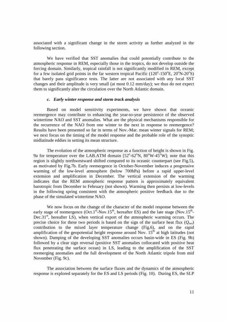
The evolution of the atmospheric response as a function of height is shown in Fig.

9a for temperature over the LAB.ATM domain [52o-62oN, 80oW-45oW]; note that this region is slightly northwestward shifted compared to its oceanic counterpart (see Fig.5), as motivated by Fig.7b. Early reemergence in October-November induces a progressive warming of the low-level atmosphere (below 700hPa) before a rapid upper-level extension and amplification in December. The vertical extension of the warming indicates that the REM atmospheric response pattern is approximately equivalent barotropic from December to February (not shown). Warming then persists at low-levels in the following spring consistent with the atmospheric positive feedback due to the phase of the simulated wintertime NAO.

We now focus on the change of the character of the model response between the

early stage of reemergence (Oct.1st-Nov.15th, hereafter ES) and the late stage (Nov.15th-Dec.31st, hereafter LS), when vertical export of the atmospheric warming occurs. The precise choice for these two periods is based on the sign of the surface heat flux (Qnet) contribution to the mixed layer temperature change (Fig.6), and on the rapid amplification of the geopotential height response around Nov. 15th at high latitudes (not shown). Damping of the developing SST anomalies occurs basin-wide in ES (Fig. 9b) followed by a clear sign reversal (positive SST anomalies collocated with positive heat flux penetrating the surface ocean) in LS, leading to the amplification of the SST reemerging anomalies and the full development of the North Atlantic tripole from mid November (Fig. 9c).

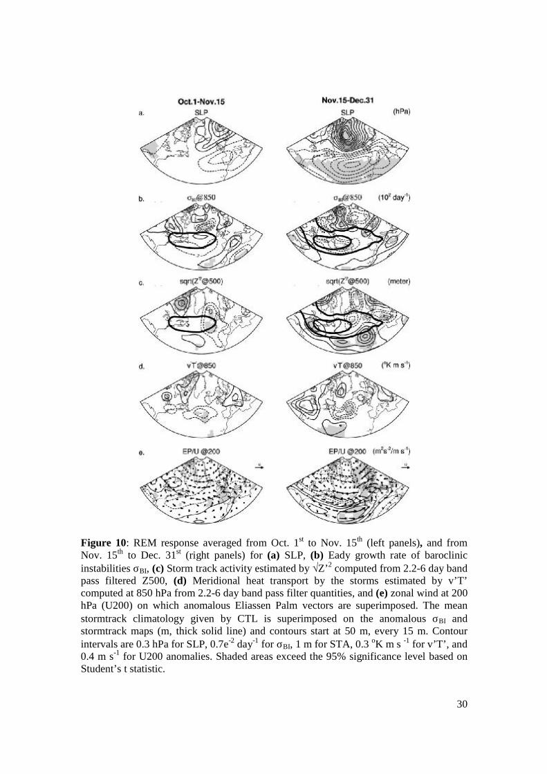
The association between the surface fluxes and the dynamics of the atmospheric response is explored separately for the ES and LS periods (Fig. 10). During ES, the SLP

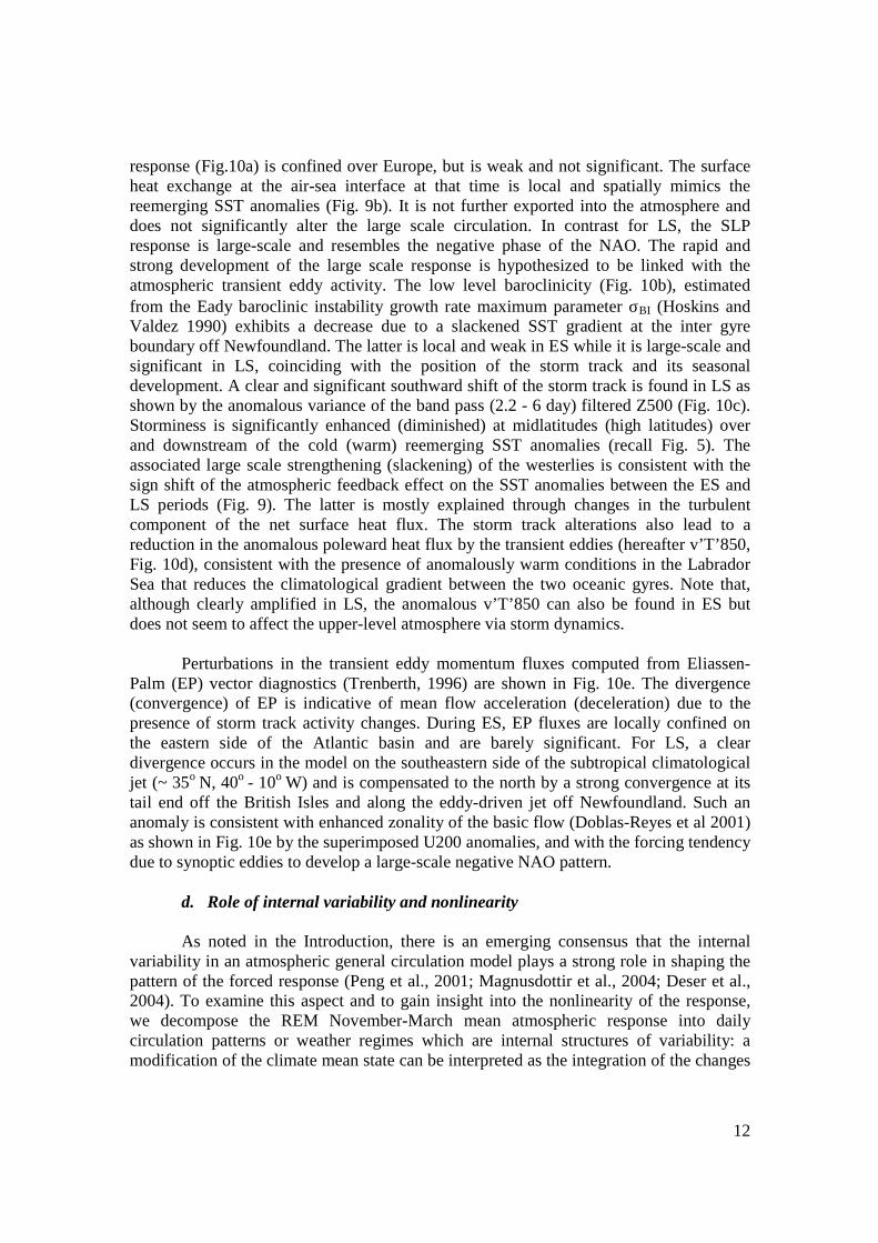
12

response (Fig.10a) is confined over Europe, but is weak and not significant. The surface heat exchange at the air-sea interface at that time is local and spatially mimics the reemerging SST anomalies (Fig. 9b). It is not further exported into the atmosphere and does not significantly alter the large scale circulation. In contrast for LS, the SLP response is large-scale and resembles the negative phase of the NAO. The rapid and strong development of the large scale response is hypothesized to be linked with the atmospheric transient eddy activity. The low level baroclinicity (Fig. 10b), estimated from the Eady baroclinic instability growth rate maximum parameter σBI (Hoskins and Valdez 1990) exhibits a decrease due to a slackened SST gradient at the inter gyre boundary off Newfoundland. The latter is local and weak in ES while it is large-scale and significant in LS, coinciding with the position of the storm track and its seasonal development. A clear and significant southward shift of the storm track is found in LS as shown by the anomalous variance of the band pass (2.2 - 6 day) filtered Z500 (Fig. 10c). Storminess is significantly enhanced (diminished) at midlatitudes (high latitudes) over and downstream of the cold (warm) reemerging SST anomalies (recall Fig. 5). The associated large scale strengthening (slackening) of the westerlies is consistent with the sign shift of the atmospheric feedback effect on the SST anomalies between the ES and LS periods (Fig. 9). The latter is mostly explained through changes in the turbulent component of the net surface heat flux. The storm track alterations also lead to a reduction in the anomalous poleward heat flux by the transient eddies (hereafter v’T’850, Fig. 10d), consistent with the presence of anomalously warm conditions in the Labrador Sea that reduces the climatological gradient between the two oceanic gyres. Note that, although clearly amplified in LS, the anomalous v’T’850 can also be found in ES but does not seem to affect the upper-level atmosphere via storm dynamics.

Perturbations in the transient eddy momentum fluxes computed from Eliassen-Palm (EP) vector diagnostics (Trenberth, 1996) are shown in Fig. 10e. The divergence (convergence) of EP is indicative of mean flow acceleration (deceleration) due to the presence of storm track activity changes. During ES, EP fluxes are locally confined on the eastern side of the Atlantic basin and are barely significant. For LS, a clear divergence occurs in the model on the southeastern side of the subtropical climatological jet (~ 35o N, 40o - 10o W) and is compensated to the north by a strong convergence at its tail end off the British Isles and along the eddy-driven jet off Newfoundland. Such an anomaly is consistent with enhanced zonality of the basic flow (Doblas-Reyes et al 2001) as shown in Fig. 10e by the superimposed U200 anomalies, and with the forcing tendency due to synoptic eddies to develop a large-scale negative NAO pattern.

d. Role of internal variability and nonlinearity As noted in the Introduction, there is an emerging consensus that the internal

variability in an atmospheric general circulation model plays a strong role in shaping the pattern of the forced response (Peng et al., 2001; Magnusdottir et al., 2004; Deser et al., 2004). To examine this aspect and to gain insight into the nonlinearity of the response, we decompose the REM November-March mean atmospheric response into daily circulation patterns or weather regimes which are internal structures of variability: a modification of the climate mean state can be interpreted as the integration of the changes

13

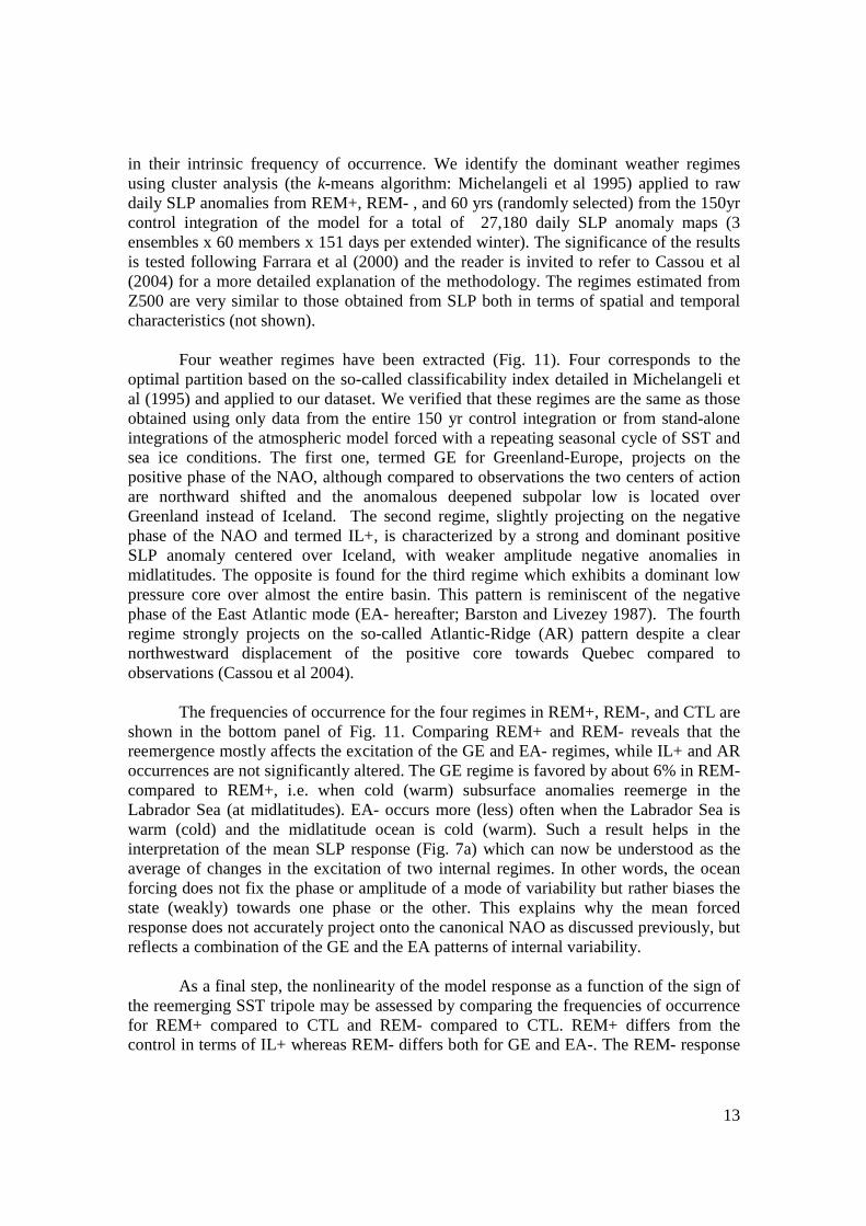
in their intrinsic frequency of occurrence. We identify the dominant weather regimes using cluster analysis (the k-means algorithm: Michelangeli et al 1995) applied to raw daily SLP anomalies from REM+, REM- , and 60 yrs (randomly selected) from the 150yr control integration of the model for a total of 27,180 daily SLP anomaly maps (3 ensembles x 60 members x 151 days per extended winter). The significance of the results is tested following Farrara et al (2000) and the reader is invited to refer to Cassou et al (2004) for a more detailed explanation of the methodology. The regimes estimated from Z500 are very similar to those obtained from SLP both in terms of spatial and temporal characteristics (not shown).

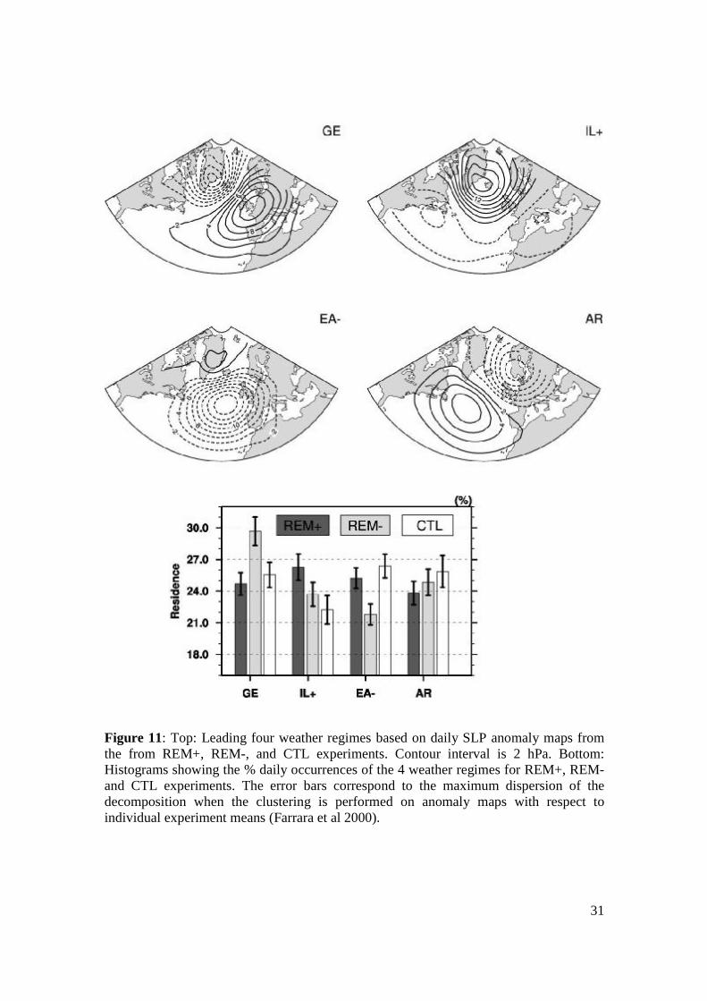
Four weather regimes have been extracted (Fig. 11). Four corresponds to the optimal partition based on the so-called classificability index detailed in Michelangeli et al (1995) and applied to our dataset. We verified that these regimes are the same as those obtained using only data from the entire 150 yr control integration or from stand-alone integrations of the atmospheric model forced with a repeating seasonal cycle of SST and sea ice conditions. The first one, termed GE for Greenland-Europe, projects on the positive phase of the NAO, although compared to observations the two centers of action are northward shifted and the anomalous deepened subpolar low is located over Greenland instead of Iceland. The second regime, slightly projecting on the negative phase of the NAO and termed IL+, is characterized by a strong and dominant positive SLP anomaly centered over Iceland, with weaker amplitude negative anomalies in midlatitudes. The opposite is found for the third regime which exhibits a dominant low pressure core over almost the entire basin. This pattern is reminiscent of the negative phase of the East Atlantic mode (EA- hereafter; Barston and Livezey 1987). The fourth regime strongly projects on the so-called Atlantic-Ridge (AR) pattern despite a clear northwestward displacement of the positive core towards Quebec compared to observations (Cassou et al 2004). The frequencies of occurrence for the four regimes in REM+, REM-, and CTL are shown in the bottom panel of Fig. 11. Comparing REM+ and REM- reveals that the reemergence mostly affects the excitation of the GE and EA- regimes, while IL+ and AR occurrences are not significantly altered. The GE regime is favored by about 6% in REM- compared to REM+, i.e. when cold (warm) subsurface anomalies reemerge in the Labrador Sea (at midlatitudes). EA- occurs more (less) often when the Labrador Sea is warm (cold) and the midlatitude ocean is cold (warm). Such a result helps in the interpretation of the mean SLP response (Fig. 7a) which can now be understood as the average of changes in the excitation of two internal regimes. In other words, the ocean forcing does not fix the phase or amplitude of a mode of variability but rather biases the state (weakly) towards one phase or the other. This explains why the mean forced response does not accurately project onto the canonical NAO as discussed previously, but reflects a combination of the GE and the EA patterns of internal variability.

As a final step, the nonlinearity of the model response as a function of the sign of the reemerging SST tripole may be assessed by comparing the frequencies of occurrence for REM+ compared to CTL and REM- compared to CTL. REM+ differs from the control in terms of IL+ whereas REM- differs both for GE and EA-. The REM- response

14

is consistent with Peng et al (2001) showing the presence of an equivalent barotropic ridge immediately downstream of the warm SST anomalies located in that case in the Labrador Sea and extending eastward. The nature of the REM+ response can be understood following the same mechanism. Warm midlatitude SST anomalies and their prolongation along the western European seaboard favor the GE regime that is characterized by raising of geopotential height surfaces above and downstream of these anomalies. At the same time, the ocean anomalies diminish the excitation of the EA- regime dominated by a trough located downstream of the anomalies, and projecting on the opposite phase of GE. The fact that different regimes are altered between REM+ and REM- is expected to be controlled by how strongly the SST-forced direct response projects on the regimes themselves, which are mostly controlled by internal eddy-driven dynamics. It is beyond the scope of this paper to examine in further detail the nonlinearity of the model response. 5. Summary and Discussion

A simplified coupled model consisting of an atmospheric GCM, an entraining ocean mixed layer model, and a thermodynamic sea ice model, has been developed to examine the impact of winter-to-winter reemergence of SST anomalies in the North Atlantic upon the atmospheric circulation. The reemergence mechanism is first evaluated in the model through a long 150-yr control integration from which we extract the dominant structure of oceanic thermal variability beneath the shallow summer mixed layer that is related to the previous late-winter atmospheric forcing. In agreement with previous studies based on observations or conceptual models, the diagnosed oceanic pattern strongly projects on the North Atlantic tripole created by the previous wintertime NAO. The associated 3-dimensional thermal anomalies are then imposed in the ocean initial conditions of two 60-member ensembles (one with positive polarity and one with negative polarity) of coupled experiments of 1-yr duration starting in August. These thermal anomalies are included between 40m and 400m (e.g., below the summer mixed layer), thus keeping the surface ocean unperturbed to mimic the reemergence framework, and north of 25oN to avoid any tropical influences. We verify in the model that the imposed thermal anomalies are re-entrained in the seasonal deepening mixed layer at the beginning of winter, and are associated with significant SST anomalies at that time.

Exposed to the reemerging oceanic thermal perturbation, the model atmosphere develops a mean quasi-barotropic response which strongly projects on the NAO. Its phase is the same as the one which generated the oceanic thermal anomalies in the previous winter, thus contributing to winter-to-winter persistence of the NAO, and the amplitude of the SLP response represents locally about 20-25% of the interannual standard deviation estimated from the control simulation. The amplitude of the reemergence induced signal is comparable to any other externally forced signal as detailed in Kushnir et al (2002) and is consistent with the absence of a robust reemergence-forced signal in atmospheric observations and in CTL. Reemergence could be important though for seasonal forecast because the oceanic process may play a major role for a given year when other forcings happen to be weak or when the previous winter NAO signature and associated subsurface ocean thermal anomalies are pronounced.

15

We speculate that transient eddies along the North Atlantic stormtrack play a significant role in shaping the structure of the large-scale atmospheric response, as well as in controlling its timing. Based on classical diagnostics, we showed a positive feedback role for the transient eddies on the mean flow, from mid-November onward. It is interesting to note that low-level atmospheric anomalies along the storm track are present at the early stage of the reemergence, whereas upper-level fields are not altered, except locally over Europe (Fig. 10). This suggests that the perturbation in the meridional SST gradient may not be exported to upper levels before mid-November because the mean circulation is not sufficiently dynamically active. This further highlights the importance of the mean seasonal flow, in particular the position and strength of the upper level jet with respect to the SST anomalies, following Peng and Robinson (2001). We note that the SST gradient itself is not significantly enhanced in mid-November, arguing against a direct SST-gradient mechanism.

Finally, we suggest that the mean winter atmospheric response can be interpreted in terms of the weather regime paradigm. We showed that the linear portion of the reemergence mechanism alters the occurrence of the positive GE regime (which projects strongly onto the positive phase of the NAO) and negative EA regime. We suggest here that adopting the regime paradigm could be of particular interest to better understand the AGCMs responses to extratropical SST anomalies that appear to be model dependent. In particular following this framework, the difference of model sensitivity may be explained by the spatial coherence between the direct SST-forced signal and the spatial properties of the regimes controlled by internal dynamics, leading to a more or less pronounced reorganization of their occurrence.

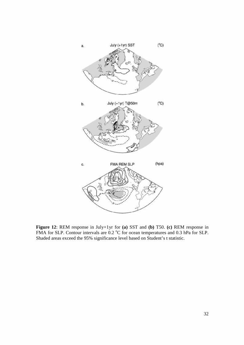
Despite the fact that we chose to apply realistic amplitude (i.e., rather weak compared to traditional studies) SST perturbations, the amplitude of the model response is detectable and comparable to that due to other sources (~ 10 – 20 m oK-1) as reviewed in Kushnir et al (2002). It would be of great interest to reproduce similar sensitivity experiments with other coupled models to better assess the robustness of the spatial pattern and magnitude of the atmospheric response to reemerging North Atlantic SST anomalies. The model response obtained here might be artificially enhanced due to biases in the CAM2 mean state: for example, the modes of variability and in particular their mid and upper-level signature, are considerably westward shifted in CAM2 compared to observations and are collocated with the regions where the imposed ocean thermal anomalies are the strongest. On the other hand, the sensitivity of the model could be considered as too conservative due to the shallower-than-observed simulated wintertime MLD, which reduces the amount of energy stored in the entire mixed oceanic column. It is interesting to note as well that the atmospheric model response presented here is strong compared to typical ones obtained from stand-alone AGCMs forced by similar amplitude SST anomalies. Given that the wintertime SLP response to the reemerging SST anomalies is of the same sign as the SLP pattern that forced the SST in the first place, to what degree will this SLP response contribute to further persisting the SST anomalies in the next winter? Figure 12 shows the temperature anomalies after 1 yr of simulation (July +1yr) at the

16

surface and at 50m depth. July+1yr SST anomalies are reminiscent of the imposed thermal anomalies but are very weak and not significant. By contrast, T50 have conserved the imprint of the thermal anomalies imposed one year earlier. These characteristics are consistent with the persistence properties of the midlatitude ocean anomalies described in the Introduction. At the surface (Fig. 12a), the summer SST anomalies generally correspond to the quasi-simultaneous forcing of the overlying atmosphere. The latter is effective at wiping out the previous winter SST anomalies as the mixed layer is very shallow and there is a decoupling between the surface and subsurface ocean. At the subsurface (Fig. 12b), anomalies as large as +0.6oC (-0.4oC) are preserved in summer in the Labrador Sea (midlatitudes) and will contribute to reemergence in the second year. These values correspond to about 25-30% of the prescribed original anomalies (see Fig. 5a) and thus appear underestimated compared to theoretical estimations (Deser et al 2003). The rapid decay of the thermal anomalies can be attributed to the winter MLD that is symptomatically too shallow in MLM but also to the late winter model response to reemergence as displayed in Fig. 12c. The FMA REM SLP response does project on the negative phase of the NAO which would contribute to the persistence of the subsurface temperature anomaly pattern, but it is northward and westward shifted compared to the original NAO circulation (see Fig. 2a for comparison) that created the imposed thermal anomalies one year earlier. Note that the amplitude of the FMA response is also rather weak and reaches at most 0.9 hPa while the FMA SLP that forced the winter SST in the first place is 5.5 hPa (the maximum value of 1.8 hPa in Fig. 2a multiplied by the maximum of the SVD PC time series). Thus, the FMA response in CTL represents a 17% positive feedback, and thus does not appear to be very efficient at further maintaining the original pattern after year 2, especially in midlatitudes. Note finally that he results of this study do not preclude at all the potential importance of the oceanic processes such as advection, diffusion, eddy mixing and subduction upon the persistence of the mixed layer temperature anomalies and the NAO. Further quantitative assessment of the effects of dynamical ocean processes versus mixed layer physics (such as the reemergence mechanism) is needed for a more complete understanding of interannual and longer timescale SST variability at midlatitudes. Acknowledgments: We thank J.W. Hurrell and L. Terray for very stimulating discussions. We are also very grateful to A.S. Phillips for its technical assistance. The figures were produced with the NCL software developed at NCAR and the simulations were carried out using the NCAR-SCD facilities under the CSL project. This work was supported in part by NOAA under Grant NA06GP0394 and by CNRS.

17

References Alexander, M. A., and C. Deser, 1995: A mechanism for the recurrence of wintertime midlatitude SST anomalies. J. Phys. Oceanogr., 25, 122-137. Alexander, M. A. and C. Penland, 1996: Variability in a mixed layer model of the upper ocean driven by stochastic atmospheric surface fluxes. J. Climate, 9, 2424-2442. Alexander, M. A., C. Deser, and M. S. Timlin, 1999: The reemergence of SST anomalies in the North Pacific Ocean. J. Climate, 12, 2419-2433. Alexander, M. A., J. D. Scott, and C. Deser, 2000: Processes that influence sea surface temperature and ocean mixed layer depth variability in a coupled model. J. Geophys. Res., 105, 16823-16842. Alexander, M. A., I. Blade, M. Newmann, J. R. Lanzante, N. C. Lau, and J. D. Scott, 2002: The atmospheric bridge: The influence of ENSO teleconnections on air-sea interaction over the global oceans. J. Climate, 15, 2205-2231. Barston, A. G., and R. E. Livezey, 1987: Classification, seasonality and persistence of low frequency atmospheric circulation patterns. Mon. Wea. Rev., 115, 1083-1126. Barsugli, J. J., and D. S. Battisti, 1998: The basic effects of atmosphere-ocean thermal coupling on midlatitude variability. J. Atmos. Sci., 55, 477-493. Briegleb, B. P., C. M. Blitz, E. C. Hunke, W. H. Lipscomb, M. M. Holland, J. L. Schramm, and R. E. Moritz, 2004: Scientific description of the sea ice component in the Community Climate System Model, Version 3. NCAR Tech. Note NCAR/TN463+STR, 70pp. Cassou, C. and L. Terray, 2001: Dual influence of Atlantic and Pacific SST anomalies on the North Atlantic/Europe winter climate. Geophys. Res. Lett., 28, 3195-3198. Cassou, C., L. Terray, J. W. Hurrell, and C. Deser, 2004: North Atlantic winter climate regimes: spatial asymmetry, stationarity with time and oceanic forcing. J. Climate, 17, 1055-1068. Cayan, D. R., 1992: Latent and sensible heat flux anomalies over the northern oceans: Driving the sea surface temperature. J. Phys. Oceanogr., 6, 249-266. de Coëtlogon, G., and C. Frankignoul, 2003: On the persistence of winter sea surface temperature in the North Atlantic. J. Climate, 16, 1364-1377. Czaja, A. and C. Frankignoul, 2002: Observed impact of Atlantic SST anomalies on the North Atlantic Oscillation. J. Climate, 15, 606-623. Czaja, A., A.W. Robertson and T. Huck, 2003: The role of Atlantic Ocean-Atmosphere coupling in affecting North Atlantic Oscillation variability. North Atlantic Oscillation: Climate Significance and Environmental Impact, Geophys. Monogr. Series, No. 134, Amer. Geophys. Union, 147-172. Delworth, T. L., 1996: North Atlantic interannual variability in a coupled ocean-atmosphere model. J. Climate, 9, 2356-2375. Deser, C., and M. S. Timlin, 1997: Atmosphere-ocean interaction on weekly timescales in the North Atlantic and Pacific. J. Climate, 10, 393-408. Deser, C., J. E. Walsh, and M. S. Timlin, 2000: Arctic sea ice variability in the context of recent atmospheric circulation trends. J. Climate, 13, 617-633. Deser, C., M. A. Alexander, and M. S. Timlin, 2003: Understanding the persistence of sea surface temperature anomalies in midlatitudes. J. Climate, 16, 57-72.

18

Doblas-Reyes, F. J., M. A. Pastor, J. M. Casado, and M. Déqué, 2001: Wintertime westward traveling planetary scale perturbations over the Euro-Atlantic region. Climate Dyn., 17, 811-824. Drévillon, M., C. Cassou, and L. Terray, 2003: Model study of the wintertime atmospheric response to fall tropical Atlantic SST anomalies. Quart. J. Roy. Meteor. Soc., 129, 2591-2611. Dong, B.-W., and R. T. Sutton 2001: The dominant mechanisms of variability in Atlantic ocean heat transport in a coupled ocean-atmosphere GCM. Geophys. Res. Lett., 28, 2445-2448. Feldstein, S. B., 2000: The timescale, power spectra and climate noise properties of the teleconnections patterns. J. Climate, 13, 4430-4440. Farrara, J. D., C. Mechoso, and A. W. Robertson, 2000: Ensembles of AGCM two-tier predictions and simulations of the circulations anomalies during winter 1997-1998. Mon. Wea. Rev, 128, 3539-3604. Frankignoul, C., and K. Hasselmann, 1977: Stochastic climate models. Part II. Application to sea surface temperature variability and thermocline variability. Tellus, 29, 289-305. Frankignoul, C., 1985: Sea surface temperature anomalies, planetary waves and air-sea feedback in middle latitudes. Rev. Geophys., 23, 357-390. Frankignoul, C., and E. Kestenare, 2002: The surface heat flux feedback. Part I. Estimates from the observations in the Atlantic and North Pacific. Climate Dyn, 19, 663-647. Gaspar, P., 1988: Modeling the seasonal cycle of the upper ocean. J. Phys. Oceanogr., 18, 161-180. Greatbach, R. T., 2000: The North Atlantic Oscillation. Stochastic and Environmental Risk Assessment, 14, 213-242. Hoskins, B. J., and P. J. Valdez, 1990: On the existence of the storm tracks. J. Atmos. Sci., 47, 1854-1864. Hurrell, J. W., 1995: Decadal trends in the North Atlantic Oscillation: regional temperatures and precipitation. Science, 269, 676-679. Hurrell, J. W., Y. Kushnir, G. Ottersen, and M. Visbeck, 2003: An overview of the North Atlantic Oscillation. North Atlantic Oscillation: Climate Significance and Environmental Impact, Geophys. Monogr. Series, No. 134, Amer. Geophys. Union, 1-22. Junge, M., and T. Haine, 2001: Mechanisms of North Atlantic wintertime sea surface temperature anomalies. J. Climate, 14, 4560-4572. Kiehl, J. T., and P. R. Gent, 2004: The community climate system model, version 2. J. Climate, 17, 3666-3682. Kushnir, Y., W. A. Robinson, I. Blade, N. M. J. Hall, S. Peng, and R. T. Sutton, 2002: Atmospheric GCM response to extratropical SST anomalies: Synthesis and evaluation. J. Climate, 15, 2233-2256. Magnusdottir, G., C. Deser, and R. Saravanan, 2004: The effects of North Atlantic SST and sea-ice anomalies on the winter circulation in CCM3, Part I: Main features and storm-track characteristics of the response. J. Climate, 17, 857-876. Michelangeli, P., R. Vautard, and B. Legras, 1995: Weather regime recurrence and quasi stationarity. J. Atmos. Sci., 52, 1237-1256.

19

Peng, S., L. A. Mysak, H. Ritchie, J. Derome, and B. Dugas, 1995: The difference between early and midwinter atmospheric responses to sea surface temperature anomalies in the northwest Atlantic. J. Climate, 8, 137-157. Peng, S. and J. Whitaker, 1999: Mechanisms determining the atmosphere response to midlatitude SST anomalies. J. Climate, 12, 1393-1408. Peng, S. and W. A. Robinson, 2001: Relationships between atmospheric internal variability and the responses to an extratropical SST anomaly. J. Climate, 14, 2943-2959. Oleson, K. W., and co-authors, 2004: Technical description of the Community Land Model (CLM). NCAR Tech. Note NCAR/TN-461+STR, 174pp. Rayner, N.A., E.C. Kent, and A. Kaplan, 2003: Global analyses of sea surface temperature, sea ice, and night marine air temperature since the late nineteenth century. J. Geophys. Res., 108, 4407, doi:10.1029/2002_JD002670. Rodwell, M. J., 2003: On the predictability of North Atlantic Climate. North Atlantic Oscillation: Climate Significance and Environmental Impact, Geophys. Monogr. Series, No. 134, Amer. Geophys. Union, 173-192. Seager, R., Y. Kushnir, M. Visbeck, N. Naik, J. Miller, G. Krahmann, and H. Cullen, 2000: Causes of Atlantic Ocean climate variability between 1958 and 1998. J. Climate, 13, 2845-2862. Stephenson, D. B., V. Pavan, and R. Bojariu, 2000: Is the North Atlantic a random walk? Int. J. Climatol., 20, 1-18. Sutton, R. T., W. A. Norton and S. P. Jewson, 2001: The North Atlantic Oscillation-What role for the ocean? Atmos. Sci. Lett., 1, 89-100. Sutton, R. T., and D. L. R. Hodson, 2005: Atlantic Ocean forcing of North America and European summer climate. Science, 309, 115-118. Terray, L. and C. Cassou, 2002: Tropical Atlantic sea surface temperature forcing of the quasi-decadal climate variability over the North Atlantic-Europe region. J. Climate, 15, 3170-3187. Timlin, M. S., M. A. Alexander, and C. Deser, 2002: On the reemergence of North Atlantic SST anomalies. J. Climate, 15, 2707-2712. Timmermann, A., M. Latif, R. Voss and A. Grötzner, 1998: Northern hemispheric interdecadal variability: a coupled air-sea mode. J. Climate, 11, 1906-1931. Trenberth, K. E., 1986: An assessment of the impact of transient eddies on the zonal flow during a blocking episode using localized Eliassen-Palm flux diagnostics. J. Atmos. Sci., 43, 2070-2087. Venske, S., M. R. Allen, R. T. Sutton, D. P. Rowell, 1999: The atmospheric response over the North Atlantic to decadal changes in sea surface temperature. J. Climate, 12, 2562-2584. von Storch, H., and F. W. Zwiers, 1999: Statistical Analysis in climate research. Cambridge University Press, 484pp. Watanabe, M., and M. Kimoto, 2000: On the persistence of decadal SST anomalies in the North Atlantic. J. Climate, 13, 3017-3028. Wunsch, C., 1999: The interpretation of short climate records, with comments on the North Atlantic Oscillation and Southern Oscillations. Bull. Amer. Meteorol. Soc., 80, 245-255.

20

Table

Season NDJ DJF JFM FMA MAM AMJ MJJ JJA JAS SCF 73 79 79 84 64 62 57 53 35 Corr. 0.50 0.62 0.62 0.59 0.45 0.64 0.64 0.61 0.37

Table 1: Squared Covariance Fraction (SCF) in percentage and correlation coefficient (Corr.) between the SVD PC time series, from lag -8 (NDJ) to 0, with ocean temperature fixed in JAS and SLP lagged as indicated. Bold stands for significance (95% level confidence) estimated following Czaja and Frankignoul (2002).

21

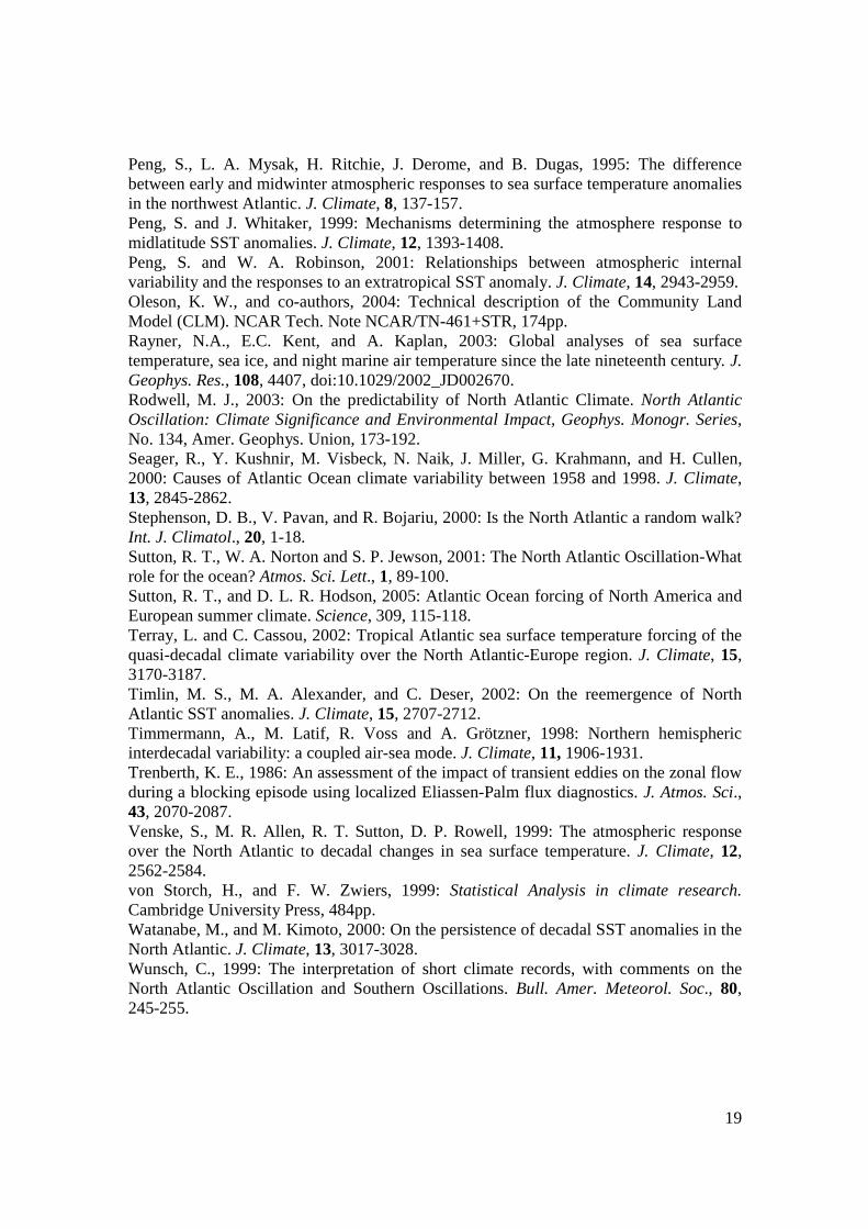
Figure 1: DJF (a) and JJA (b) average surface heat flux correction (W m2). Positive values indicate heat is added to the ocean. Shading interval is 25 W m2. CTL mean SST bias (oC) for DJF (c) and JJA (d) average given by the difference between the 150-yr mean climatology of CTL SST and the climatology of HadiSST SST over 1950-1999. The latter period corresponds to the one used to force CAM whose daily surface fluxes were then subsequently used to compute the CTL flux correction terms. Shading interval is 0.3oC. 150-yr climatology of simulated sea ice fraction for CTL (shading), for DJF (e) and JJA (f) average. The 0.5 limit for the HadiSST sea ice climatology is superimposed (purple thick line). Shading interval is 0.1. Simulated maximum mixed layer depth (m) for boreal (g) and austral (h) winter. Note that the shading interval changes with depth: 25m for MLD<100, 50m for 100<MLD<300, and 200m for deeper MLD.

22

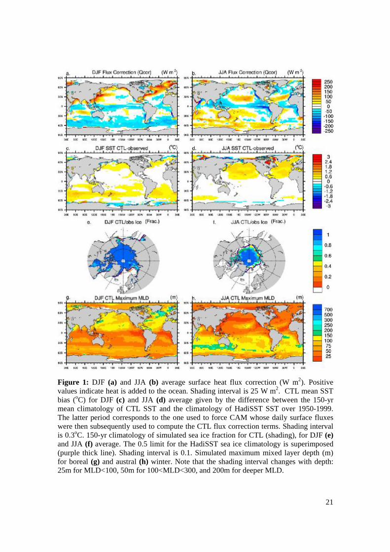
Figure 2: Leading SVD modes calculated between FMA SLP (hPa) and JAS ocean temperature (T) anomalies (oC) between 40m and 400m depth, computed from the 150-yr CTL simulation. The heterogeneous SLP anomaly pattern is shown in a) and a representative depth (50 m) of the homogeneous ocean T anomaly pattern is shown in b) to preserve the linear relationship between the variables (Czaja and Frankignoul 2002). Contour intervals are 0.3 hPa and 0.05oC, respectively. (c) Corresponding normalized principal component time series of FMA SLP (solid line) and JAS subsurface temperature (bars).

23

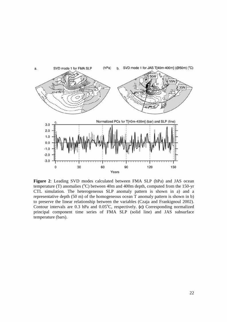
Figure 3: Simulated CTL lead-lag correlations between the March ocean temperature anomalies averaged over 50o-60oN/60o-30oW and the first upper 30m (dashed box), and temperature anomalies between the surface and 450m, from the previous Feb. through the following Feb. Contour interval is 0.05 and values in excess of 0.65 are shaded to highlight the reemergence mechanism. The thick superimposed solid line represents the 150-yr climatological mean of the MLD averaged over the domain.

24

Figure 4: Anomalous 3 dimensional temperature patterns (oC) added to (subtracted from) Aug. 1st initial oceanic conditions for REM+ (REM-) and represented here for 3 ocean sections given in the lower right corner (drawn in Fig. 2b), as a function of depth. The solid (dashed) thick black line stands for the climatological August (January) MLD simulated in CTL. Contour interval is 0.1oC.

25

Figure 5: Temporal evolution of the REM temperature anomalies (oC) at 50 m depth (left panels) and at the surface (right panels) from Sept. to March. Contour interval is 0.2oC. LAB [50o-60oN, 60oW-30oW] and MID [30o-45oN, 75oW-45oW] domains used subsequently for oceanic averaged fields are shown on the March T50 lower right panel.

26

Figure 6: Temporal evolution (from Aug. 1st to Apr. 1st) of the simulated REM anomalies averaged over the (a) LAB.OCE and (b) MID.OCE oceanic domains for temperature anomalies at 50 m depth (T50; thick grey) and SST (dashed grey), and for the mixed layer heating rate (see equation 1) due to entrainment (Qwe, solid thin black line) and due to surface fluxes (Qnet, dashed thin black line). A 15-day running mean has been applied to Q quantities, and units are oC and 1.e-7 oC/day, respectively.

27

Figure 7: REM response in NDJFM for (a) SLP, (b) T850, (d) Z500, and (e) U200. The mean U200 climatology given by CTL is superimposed (m s-1, thick solid line) and contours start at 30 m s-1, every 10 m s-1. Contour intervals are 0.3 hPa for SLP, 0.1 oC for T850, 2 m for Z500 and 0.4 m s-1 for U200 anomalies. Shaded areas exceed the 95% significance level based on Student’s t statistic. (c) REM sea ice response for JFM (grey shading for decrease, dotting for increase fraction) on which REM surface wind response is superimposed.

28

Figure 8: Leading EOF of NDJFM SLP (a) and Z500 (c) computed from the 150-yr CTL integration. Contour intervals are 0.4 hPa and 2 m, respectively. The variance explained by the EOF is given in the upper-right corner of the pattern (%). (b) Ratio between the NDJFM REM/2 SLP response and the standard deviation of NDJFM SLP computed from CTL. The REM response can be considered as a biased estimated of the reemerging SST-forced signal and the ratio can be interpreted as an averaged measure of the reemergence contribution in the CTL NDJFM interannual variability of SLP. Shading is the same as in Fig. 7a, and contour intervals are 4% starting from 8%.

29

Figure 9: (a) Temporal evolution as a function of height of the monthly REM response for temperature (oC) spatially averaged over the LAB.ATM [52o-62oN, 80oW-45oW] domain. REM response for total heat flux at the surface (W.m-2, color shading) and superimposed REM SST anomalies (oC, green (purple) contour for positive (negative) values, contour interval is every 0.2 oC) averaged from Oct. 1st to Nov. 15th (b), and from Nov. 15th to Dec. 31st (c).

30

Figure 10: REM response averaged from Oct. 1st to Nov. 15th (left panels), and from Nov. 15th to Dec. 31st (right panels) for (a) SLP, (b) Eady growth rate of baroclinic instabilities σBI, (c) Storm track activity estimated by √Z’2 computed from 2.2-6 day band pass filtered Z500, (d) Meridional heat transport by the storms estimated by v’T’ computed at 850 hPa from 2.2-6 day band pass filter quantities, and (e) zonal wind at 200 hPa (U200) on which anomalous Eliassen Palm vectors are superimposed. The mean stormtrack climatology given by CTL is superimposed on the anomalous σBI and stormtrack maps (m, thick solid line) and contours start at 50 m, every 15 m. Contour intervals are 0.3 hPa for SLP, 0.7e-2 day-1 for σBI, 1 m for STA, 0.3 oK m s -1 for v’T’, and 0.4 m s-1 for U200 anomalies. Shaded areas exceed the 95% significance level based on Student’s t statistic.

31

Figure 11: Top: Leading four weather regimes based on daily SLP anomaly maps from the from REM+, REM-, and CTL experiments. Contour interval is 2 hPa. Bottom: Histograms showing the % daily occurrences of the 4 weather regimes for REM+, REM- and CTL experiments. The error bars correspond to the maximum dispersion of the decomposition when the clustering is performed on anomaly maps with respect to individual experiment means (Farrara et al 2000).

32

Figure 12: REM response in July+1yr for (a) SST and (b) T50. (c) REM response in FMA for SLP. Contour intervals are 0.2 oC for ocean temperatures and 0.3 hPa for SLP. Shaded areas exceed the 95% significance level based on Student’s t statistic.