investigating the potential use of aerial line transect

MARINE MAMMAL SCIENCE, 29(3): 389–406 (July 2013)2012 by the Society for Marine MammalogyPublished 2012. This article is a US Government work and is in the public domain in the USA.DOI: 10.1111/j.1748-7692.2012.00574.x

Investigating the potential use of aerial line transectsurveys for estimating polar bear abundance in sea ice

habitats: A case study for the Chukchi SeaRYAN M. NIELSON,1 Western EcoSystems Technology, Inc., 200 S. Second Street, Suite B, Laramie,Wyoming 82070, U.S.A., THOMAS J. EVANS, United States Fish and Wildlife Service, MarineMammals Management, 1011 East Tudor Road, MS 341, Anchorage, Alaska 99503, U.S.A.,MICHELLE BOURASSA STAHL, Western EcoSystems Technology, Inc., 200 S. Second Street, SuiteB, Laramie, Wyoming 82070, U.S.A.

ABSTRACT

The expense of traditional capture-recapture methods, interest in less invasivesurvey methods, and the circumpolar decline of polar bear (Ursus maritimus) habitatrequire evaluation of alternative methods for monitoring polar bear populations.Aerial line transect distance sampling (DS) surveys are thought to be a promisingmonitoring tool. However, low densities and few observations during a survey canresult in low precision, and logistical constraints such as heavy ice and fuel andsafety limitations may restrict survey coverage. We used simulations to investigatethe accuracy and precision of, DS for estimating polar bear abundance in sea icehabitats, using the Chukchi Sea subpopulation as an example. Simulation parame-ters were informed from a recent pilot survey. Predictions from a resource selectionmodel were used for stratification, and we compared two ratio estimators to accountfor areas that cannot be sampled. The ratio estimator using predictions of resourceselection by polar bears allowed for extrapolation beyond sampled areas and pro-vided results with low bias and CVs ranging from 21% to 36% when abundancewas >1,000. These techniques could be applied to other DS surveys to allocateeffort and potentially extrapolate estimates to include portions of the landscape thatare logistically impossible to survey.

Key words: Chukchi Sea, distance sampling, line transect, polar bear, Ursusmaritimus, population size, resource selection, sea ice, stratification.

To date, there are few reliable abundance estimates for many of the polar bear(Ursus maritimus) subpopulations currently recognized by the International Unionfor the Conservation of Nature and Natural Resources (IUCN) Polar Bear SpecialistGroup (PBSG; Aars et al. 2006), including the subpopulation occupying the ChukchiSea. The Chukchi Sea polar bear subpopulation occurs primarily in the Chukchi Seaand Bering Sea, and management is shared between the United States (Alaska) andRussia. The majority of the Chukchi Sea polar bear subpopulation remains on the ice

1Corresponding author (e-mail: [email protected]).

389

390 MARINE MAMMAL SCIENCE, VOL. 29, NO. 3, 2013

year-round and inhabit large remote oceanic areas that are not accessible to land-basedhelicopters. The Chukchi Sea subpopulation also overlaps with the Southern BeaufortSea subpopulation in northwestern Alaska. The Agreement between the UnitedStates of America and the Russian Federation on the Conservation and Managementof the Alaska-Chukotka Polar Bear Population (Bilateral Agreement) became law in2006 and was established in part to develop an effective unified management systembetween the two countries. Monitoring abundance of the Chukchi Sea subpopulationis necessary due to the intense interest in polar bear management following the listingof polar bears as threatened under the Endangered Species Act (ESA) on 15 May 2008(U.S. Federal Register 73 FR 28212), concerns over overharvest, and the potentialeffects of global climate change on polar bear sea ice habitat (Durner et al. 2009).

Due to the invasiveness, high cost and sample size requirements of a capture–recapture study, aerial line transect distance sampling (DS; Buckland et al. 2001)methodology may provide a promising alternative for estimating polar bear abun-dance (Wiig and Derocher 1999, Aars et al. 2009). The main advantages of DSsurveys are that they are less invasive and can be completed in a much shorter periodof time. However, in addition to the relatively low density of polar bears in theregion, there are many logistical constraints such as limited access to remote areasfar offshore, the limited range of helicopters, and dynamic sea ice conditions thatcould complicate obtaining a reliable polar bear abundance estimate using DS forthe Chukchi Sea subpopulation. It has been estimated that each autumn 150–600polar bears from the Chukchi Sea subpopulation come on land on Wrangel Island(Ovsyanikov and Menyushina 2010) and an additional 20 or more bears come onland on the Chukotkan coast (Kochnev 2005). Regular surveys along the US coasthave not been conducted, but it is believed that few bears occur on land in theUnited States during the autumn. This study focuses on methodology to estimatethe abundance of the polar bears in sea ice habitats as part of a larger, multisurveyeffort of land and sea ice habitats that would be needed to estimate the size of theChukchi Sea subpopulation.

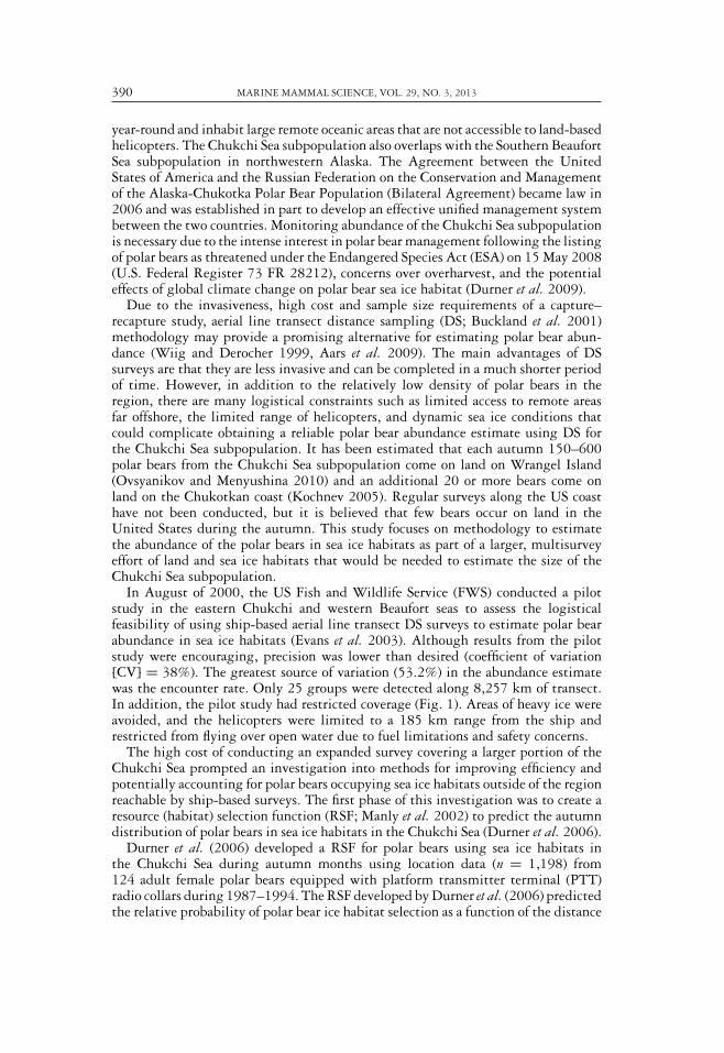
In August of 2000, the US Fish and Wildlife Service (FWS) conducted a pilotstudy in the eastern Chukchi and western Beaufort seas to assess the logisticalfeasibility of using ship-based aerial line transect DS surveys to estimate polar bearabundance in sea ice habitats (Evans et al. 2003). Although results from the pilotstudy were encouraging, precision was lower than desired (coefficient of variation[CV] = 38%). The greatest source of variation (53.2%) in the abundance estimatewas the encounter rate. Only 25 groups were detected along 8,257 km of transect.In addition, the pilot study had restricted coverage (Fig. 1). Areas of heavy ice wereavoided, and the helicopters were limited to a 185 km range from the ship andrestricted from flying over open water due to fuel limitations and safety concerns.

The high cost of conducting an expanded survey covering a larger portion of theChukchi Sea prompted an investigation into methods for improving efficiency andpotentially accounting for polar bears occupying sea ice habitats outside of the regionreachable by ship-based surveys. The first phase of this investigation was to create aresource (habitat) selection function (RSF; Manly et al. 2002) to predict the autumndistribution of polar bears in sea ice habitats in the Chukchi Sea (Durner et al. 2006).

Durner et al. (2006) developed a RSF for polar bears using sea ice habitats inthe Chukchi Sea during autumn months using location data (n = 1,198) from124 adult female polar bears equipped with platform transmitter terminal (PTT)radio collars during 1987–1994. The RSF developed by Durner et al. (2006) predictedthe relative probability of polar bear ice habitat selection as a function of the distance

NIELSON ET AL.: ESTIMATING POLAR BEAR ABUNDANCE 391

Figure 1. Study area, flight lines, and polar bear observations in the eastern Chukchi Seaand western Beaufort Sea off northern Alaska during August 2000 (pilot study; fig. 1 in Evanset al. 2003).

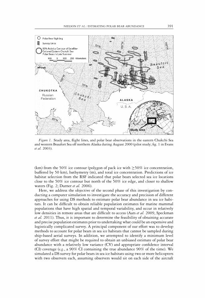
(km) from the 50% ice contour (polygon of pack ice with ≥50% ice concentration,buffered by 50 km), bathymetry (m), and total ice concentration. Predictions of icehabitat selection from the RSF indicated that polar bears selected sea ice locationsclose to the 50% ice contour but north of the 50% ice edge, and closer to shallowwaters (Fig. 2; Durner et al. 2006).

Here, we address the objective of the second phase of this investigation by con-ducting a computer simulation to investigate the accuracy and precision of differentapproaches for using DS methods to estimate polar bear abundance in sea ice habi-tats. It can be difficult to obtain reliable population estimates for marine mammalpopulations that have high spatial and temporal variability, and occur in relativelylow densities in remote areas that are difficult to access (Aars et al. 2009, Speckmanet al. 2011). Thus, it is important to determine the feasibility of obtaining accurateand precise population estimates prior to undertaking what could be an expensive andlogistically complicated survey. A principal component of our effort was to developmethods to account for polar bears in sea ice habitats that cannot be sampled duringship-based aerial surveys. In addition, we attempted to identify a minimum levelof survey effort that might be required to obtain an unbiased estimate of polar bearabundance with a relatively low variance (CV) and appropriate confidence interval(CI) coverage (e.g., a 90% CI containing the true abundance 90% of the time). Wesimulated a DS survey for polar bears in sea ice habitats using two or more helicopterswith two observers each, assuming observers would sit on each side of the aircraft


Figure 2. Resource selection function (RSF) distribution map for 15 October 1990, withlocations of GPS collared polar bears. RSF intervals represent 5% of the landscape. RSF interval1 represents the areas with the lowest relative probability of polar bear habitat selection, andinterval 20 represents the 5% of the landscape with the highest relative probability of selection.The white polygon represents Wrangel Island, Russia.

in the rear seats. We also assumed that future surveys would follow survey protocoldescribed by Evans et al. (2003).

METHODS

Study Area

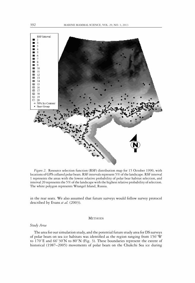
The area for our simulation study, and the potential future study area for DS surveysof polar bears on sea ice habitats was identified as the region ranging from 156◦Wto 170◦E and 66◦30′N to 80◦N (Fig. 3). These boundaries represent the extent ofhistorical (1987–2005) movements of polar bears on the Chukchi Sea ice during


Figure 3. Boundary of the full Chukchi Sea study area used in the simulation.

15 September to 14 November, based on relocations of radio-tagged individuals(Durner et al. 2006). Polar bears from the Chukchi Sea subpopulation typicallyfollow the movement of the ice as it increases during the winter months and recedesduring the summer (Garner et al. 1990, 1994). During the late summer and earlyfall, the recession of the Arctic sea ice reaches its maximum. The autumn surveyperiod was chosen because minimal sea ice extent occurs at that time throughout theArctic, and bears that remain on the ice are typically concentrated near the recedingice edge.

Overview of Simulations

Our simulations were designed to mimic historic sea ice conditions, practicalsurvey protocols, and logistical constraints similar to the pilot study (Evans et al.2003). We considered 4, 6, and 8 week-long survey periods in the simulations, andsubpopulation sizes of 500, 1,000, 2,000, 2,500, and 3,000 polar bears occupyingthe sea ice within the study area. To ensure that we accounted for changing seaice conditions in our simulations, we used daily passive microwave sea ice data tomodel ship movement, where DS could occur each day, and hypothetical polar bearlocations.

Step 1. Randomly select a survey year and start time—For each replication in a simula-tion, a year from 1985 to 1994 was selected at random, along with a random startingdate for DS survey that allowed for completion of the survey by 14 November. Thesedates represent the time period used by Durner et al. (2006) to develop the RSF inthe first phase of this investigation. On the first day of each simulated survey, theship was randomly placed in a 5 × 5 km cell within 8 km of the western ice edge in


the study region (Russian waters), and as close to the 50% ice contour as possible.The daily passive microwave sea ice data from subsequent dates in that year werethen used to represent ice conditions in the simulation in order to mimic realisticchanges over the course of a survey.

Step 2. Simulate daily survey area—The daily survey area was restricted by two fac-tors. First, the sea ice data used in this investigation was based on passive microwaveimagery (SSMR, SSM/I; National Snow and Ice Data Center [NSIDC], Boulder, CO).These data were originally in raster format with a pixel size of 25 × 25 km, butresampled at a 5 × 5 km resolution. Because passive microwave data are not reliablealong shorelines (Cavalieri et al. 1999), we excluded pixels that were within 25 kmof land. A rasterized land mask (1:10 scale Digital Chart of the World; DefenseMapping Agency 1992) with a 25 km buffer effectively removed most of the coastalpixels. Second, the area sampled in the simulations was allowed to vary by day ac-cording to sea ice characteristics. Ship-based aerial surveys would be limited by theextent and concentration of sea ice, with daily variation due to the effects of windand current. Icebreakers available for such a survey cannot efficiently travel throughice dominated waters, and areas of heavy ice are usually avoided (Evans et al. 2003).In addition, helicopter surveys sponsored by the FWS are not permitted over openwater and have a limited range.

We defined the southern boundary of the daily survey area as the southern extentof sea ice on that day. The resolution of the passive microwave satellite imagerymeant that some pixels classified as “open water” may have contained undetectedsea ice. To account for this lack of precision, we buffered areas of pack ice recordedwith ≥15% ice concentration by 50 km. We then retained the single, very largepolygon of pack ice within this area (Durner et al. 2006). This polygon containedthe 50% ice edge described above. Consequently, any small parcels (islands) of seaice south of the main pack were not included in the daily survey area. The peripheryof the single large polygon was considered the edge of the main ice pack, and ishereafter termed the 15% ice contour.

Step 3. Simulate polar bear locations—The RSF was applied to the daily ice conditionsto estimate daily RSF intervals (e.g., 0%–10% relative probability of use, 11%–20%,etc.). Hypothetical polar bear groups were placed within the study area on each surveyday. This was done by sampling 5 × 5 km cells in the study area, with replacement,using a non-equal probability sampling scheme. Sampling weights were based on theproportion of historical polar bear locations (n = 1,862) in each RSF interval (Durneret al. 2006; e.g., Fig. 2). Thus, 5 × 5 km cells containing polar bears were clumpedand not uniformly distributed across the sea ice. However, the exact location of polarbear groups within each 5 × 5 km cell was random. This method of modelingpolar bear locations is based on empirical data and should mimic reality if the RSFdeveloped by Durner et al. (2006) accurately predicts where polar bears will be inthe future under changing sea ice conditions.

A number (45) of the simulated locations were randomly designated as polar bearsequipped with GPS radio telemetry collars. We believed it would be reasonable tocapture 20 adult female polar bears on a yearly basis prior to a DS survey, and iftelemetry collars were designed for a 2 yr deployment, we could expect approximately45 collared bears to be present during the survey. The locations of these bears wereused in the analysis to account for individuals outside of the area reachable by aship-based aerial survey (see Step 9).

Step 4. Simulate polar bear group sizes—Polar bear group sizes were generated byadding 1.0 to a random value from a Poisson distribution with a mean of � = 0.16.


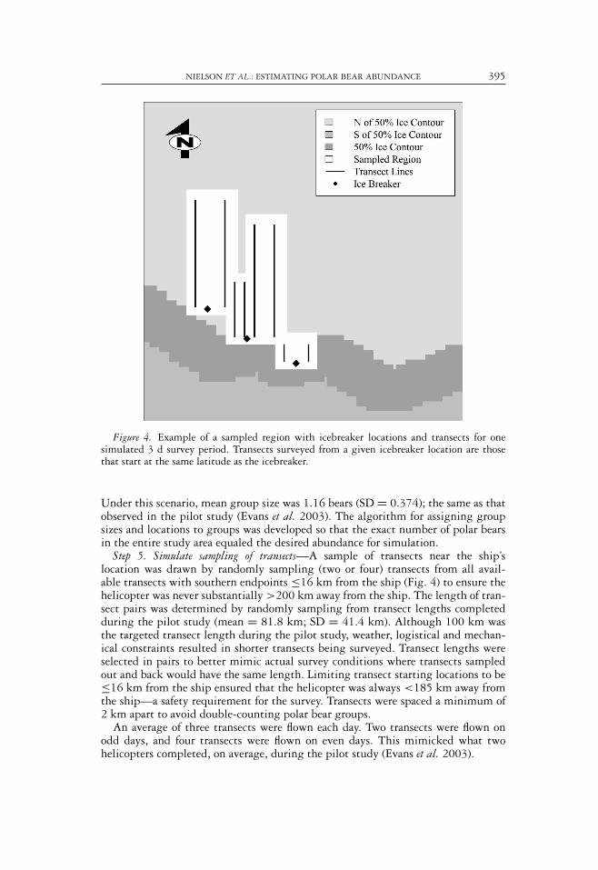
Figure 4. Example of a sampled region with icebreaker locations and transects for onesimulated 3 d survey period. Transects surveyed from a given icebreaker location are thosethat start at the same latitude as the icebreaker.

Under this scenario, mean group size was 1.16 bears (SD = 0.374); the same as thatobserved in the pilot study (Evans et al. 2003). The algorithm for assigning groupsizes and locations to groups was developed so that the exact number of polar bearsin the entire study area equaled the desired abundance for simulation.

Step 5. Simulate sampling of transects—A sample of transects near the ship’slocation was drawn by randomly sampling (two or four) transects from all avail-able transects with southern endpoints ≤16 km from the ship (Fig. 4) to ensure thehelicopter was never substantially >200 km away from the ship. The length of tran-sect pairs was determined by randomly sampling from transect lengths completedduring the pilot study (mean = 81.8 km; SD = 41.4 km). Although 100 km wasthe targeted transect length during the pilot study, weather, logistical and mechan-ical constraints resulted in shorter transects being surveyed. Transect lengths wereselected in pairs to better mimic actual survey conditions where transects sampledout and back would have the same length. Limiting transect starting locations to be≤16 km from the ship ensured that the helicopter was always <185 km away fromthe ship—a safety requirement for the survey. Transects were spaced a minimum of2 km apart to avoid double-counting polar bear groups.

An average of three transects were flown each day. Two transects were flown onodd days, and four transects were flown on even days. This mimicked what twohelicopters completed, on average, during the pilot study (Evans et al. 2003).


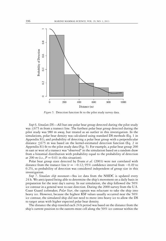
Figure 5. Detection function fit to the pilot study survey data.

Step 6. Simulate DS—All but one polar bear group detected during the pilot studywas ≤675 m from a transect line. The furthest polar bear group detected during thepilot study was 980 m away, but treated as an outlier in this investigation. In thesimulations, polar bear density was calculated using standard DS methods (Eq. 1 inAppendix S1), and probability of detecting a polar bear group with a perpendiculardistance ≤675 m was based on the kernel-estimated detection function (Eq. 2 inAppendix S1) fit to the pilot study data (Fig. 5). For example, a polar bear group 200m east or west of a transect was "observed" in the simulation based on a random drawfrom a binomial distribution with probability equal to the probability of detectionat 200 m (i.e., P = 0.61 in this situation).

Polar bear group sizes detected by Evans et al. (2003) were not correlated withdistance from the transect line (r = −0.12; 95% confidence interval from −0.49 to0.25), so probability of detection was considered independent of group size in thisinvestigation.

Step 7. Simulate ship movement—Sea ice data from the NSIDC is updated every24 h. We anticipated being able to determine the ship’s movement on a daily basis inpreparation for the next day’s survey. In our simulation, the ship followed the 50%ice contour in a general west to east direction. During the 2000 survey from the U.S.Coast Guard icebreaker, Polar Star, the captain was reluctant to take the ship intoheavy ice. However, because the highest RSF values usually occurred near the 50%ice contour, the simulated ship did not need to move into heavy ice to allow the DSto target areas with higher expected polar bear density.

The distance the ship traveled each 24 h period was based on the distance from theship’s current position to the eastern-most cell along the 50% ice contour within the


study region and the number of remaining survey days. For example, if the distancefrom the ship to the eastern-most cell containing the 50% ice contour was 1,000 km,and there were 19 d left in the survey, the ship was moved 1,000/(19 + 1) = 50 kmto the east and as close to the 50% ice contour as possible in preparation for the nextday’s survey. The maximum distance the ship was allowed to travel in any one daywas capped at 80 km, which was the maximum distanced traveled during the pilotstudy (Evans et al. 2003). This algorithm moved the ship at a somewhat consistentpace, allowed complete west to east coverage of the study area, and prevented thesurvey from reaching the eastern edge of the study area before the survey periodelapsed.

Step 8. Repeat steps 2–7—Steps 2 through 7 were repeated until the end of thesurvey period. Based on an average of 3 transects surveyed each day, this amountedto 84, 126, and 168 transects surveyed during the 4,6, and 8 wk simulated surveyperiods, respectively.

Step 9. Estimate abundance based on simulated data—Two issues related to conductingDS over sea ice complicate standard analyses. First, standard DS analyses assumethe density of objects is constant during the study period (Buckland et al. 2001).However, even if the number of polar bears in the study area is constant during asurvey period, polar bear density is expected to decrease over time due to expansionthe area of available sea ice, i.e., as the sea ice surface extent increases polar beardensity on the ice surface decreases. For example, the extent of ice in the Chukchi Seanearly doubled (92% increase) from 15 September to 14 November in 1993 (Durneret al. 2006) while the number of bears in the area remained essentially constant.Second, we cannot expect to obtain a spatially representative sample of transectsthroughout the study area due to limitations of ship-based aerial surveys (Evans et al.2003). This presents a major hurdle in estimation of polar bear abundance in the seaice habitats, because polar bear density is not expected to be homogeneous (Durneret al. 2006, 2009).

To overcome the issue of an increasing sea ice extent and the resulting decrease inpolar bear density we divided the survey into 3 d segments, or survey periods (i.e.,days 1–3, days 4–6, etc.), and estimated the polar bear abundance in the study areaduring each 3 d period. After estimating the total number of polar bears on the seaice within the study region for each 3 d period, we averaged the 3 d period estimatesfor our final estimate of total abundance.

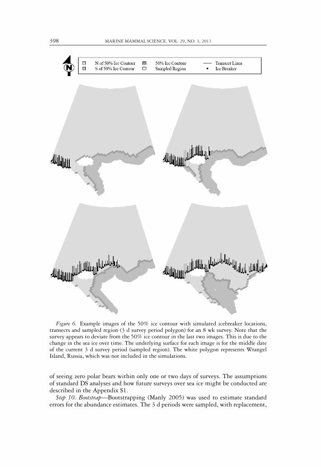
We used all observations among survey periods to estimate a detection functionand the average group size, but the total number of detected polar bear groups (n)and total length of transect lines flown during a 3 d period were used to obtain anestimate of the density of polar bears in the area searched during those three days(see Appendix S1). We then estimated the total number of polar bears occupyingthe sampled region during the 3 d period by connecting the northern and southernendpoints of each transect surveyed (Fig. 6). This polygon constituted the regionsampled during the 3 d period, and total abundance was estimated for this polygon.

To account for polar bears outside of the region sampled (polygon) during each3 d period, we considered two extrapolation methods. The first method used theratio of collared bears to the estimated total abundance in the study region (Eq. 3 inAppendix S1). The second method involved the ratio of areas under the RSF surface(Eq. 4 in Appendix S1). Use of both ratio estimators required assuming that the seaice and distribution of polar bears was constant within each survey period. Thus, wefelt three days was the maximum length of time that could be used for each surveyperiod. In addition, we did not use a shorter survey period because of the likelihood


Figure 6. Example images of the 50% ice contour with simulated icebreaker locations,transects and sampled region (3 d survey period polygon) for an 8 wk survey. Note that thesurvey appears to deviate from the 50% ice contour in the last two images. This is due to thechange in the sea ice over time. The underlying surface for each image is for the middle dateof the current 3 d survey period (sampled region). The white polygon represents WrangelIsland, Russia, which was not included in the simulations.

of seeing zero polar bears within only one or two days of surveys. The assumptionsof standard DS analyses and how future surveys over sea ice might be conducted aredescribed in the Appendix S1.

Step 10. Bootstrap—Bootstrapping (Manly 2005) was used to estimate standarderrors for the abundance estimates. The 3 d periods were sampled, with replacement,


for each of 200 bootstrap samples. Each bootstrap sample contained the originalnumber of 3 d periods in the simulated survey. New estimates of polar bear abundancewere calculated for each bootstrap sample. The standard error for total abundancewas estimated as the standard deviation of the 200 bootstrap estimates, and 90%CIs were calculated using N̂ ± 1.645 × SE[N̂]. The primary sample units in ouranalysis are the 3 d survey periods (Step 9), so when calculating CIs, it is conservative(CIs are wider) to bootstrap the 3 d period estimates of abundance rather than theindividual transects. This method does not account for the variability in the RSFsurface, which we expect to be of minor significance.

Step 11. Repeat steps 1–10—Steps 1 through 10 were repeated 500 times for eachcombination of abundance and survey period length.

Step 12. Compute summary statistics based on simulation results—We calculated the%CV, and the percent coverage of a 90% CI for each combination of abundance andsurvey period length. Overall, the objectives are to minimize the %CV and have a90% CI contain the true abundance approximately 90% of the time.

All simulation steps were conducted in R (R Development Core Team 2008).

Survey Costs

We evaluated the relative cost of DS compared to capture-recapture studies.The costs for capture-recapture efforts in Alaska and Russia were based on ongo-ing capture-recapture studies in Alaska and draft research proposals for conductingground-based studies in Chukotka, Russia. Typically, most capture-recapture effortshave taken place from land-based logistic centers, and although ice-breakers could beused for capture-recapture efforts we did not consider this option when evaluating therelative costs. In addition, the use of genetic samples collected through biopsy dart-ing and hair snares, which are alternative capture-recapture methods for estimatingabundance, were not considered in this evaluation. We assumed that sampling wouldhave to occur in at least one location in each country and that a 5 yr time frame wouldbe sufficient for obtaining a population estimate from a capture-recapture study.

Line transect survey cost estimates were based the cost of a U.S. Coast Guardicebreaker with the ability to support two helicopters during the DS survey. Costestimates for concurrent aerial surveys along the coastline of Alaska and Chukotka,Russia, were based on previous surveys and cost estimates provided by our Russiancolleagues.

RESULTS

In simulations where surveys lasted eight weeks, the ship moved between 11 and79 km each day (median = 25.0). During the course of 6 wk surveys, the ship movedbetween 20.0 and 79.1 km each day (median = 32.0). For 4 wk surveys, the shipmoved between 30.4 and 79.1 km each day (median = 47.2).

Simulation results of primary interest (population estimates) are presented in Table1. In general, the abundance estimator based on the area under the RSF surface (RSFestimator; Eq. 4 in Appendix S1) had a CV < 36% when abundance was >1,000,and 90% CI coverage was ≥86% for abundances ≥1,000. The average relative sizeof a 90% CI was plus/minus 66%, 41%, 37%, and 34% when abundance was 1,000,2,000, 2,500, and 3,000, respectively. Bias for this estimator was generally <10%when the abundance was ≥2,000, but became larger as abundance decreased. The


Table 1. Average estimate of the number of polar bears in the Chukchi Sea, percent coverageof a 90% confidence interval (CI), and the average coefficient of variation (CV = SE/estimate)for two estimators of abundance, for each hypothetical subpopulation size and number ofsurvey weeks considered in the simulations. Simulations had 45 bears equipped with radiotelemetry collars, and flew an average of three transects per day. A 90% confidence intervalshould contain the true population size 90% of the time (i.e., CI Coverage = 90%). Theaverage size of the 90% CIs could be approximated for each simulation using ±1.645 × CV.

Ratio of collared bears RSF surface– –

Abundance Survey weeks�

N CI coverage C V�

N CI coverage C V

3,000 8 1,958 38% 28% 3,118 91% 21%6 2,161 54% 30% 3,009 87% 23%4 2,719 73% 35% 3,195 86% 29%

2,500 8 1,592 36% 29% 2,583 91% 23%6 1,857 56% 32% 2,618 89% 24%4 2,218 72% 39% 2,753 87% 34%

2,000 8 1,405 54% 32% 2,271 91% 25%6 1,550 64% 35% 2,184 90% 28%4 1,744 72% 40% 2,229 87% 36%

1,000 8 856 76% 46% 1,397 91% 40%6 966 79% 46% 1,381 89% 42%4 1,246 80% 48% 1,526 86% 45%

500 8 630 90% 46% 1,098 59% 43%6 712 78% 36% 1,066 44% 33%4 887 61% 29% 1,201 34% 27%

8 wk simulation with 3,000 bears had the best performance with a CV of 21% anda 90% CI coverage of 91%. Decreasing the length of the survey, and thus numberof transects flown, resulted in a small increase in the CV and a slight decrease in the90% CI coverage. Similarly, decreasing the number of bears on the sea ice resultedin poorer performance as indicated by an increase in the CV and a decrease in CIcoverage.

Performance of the estimator using the ratio of collared bears in the surveyedregion (Eq. 3 in Appendix S1) was poor under all conditions simulated (Table 1).This estimator was usually biased low (by 11%–30%) when the abundance was≥2,000. However, the estimator was biased high for an abundance of 500. Coverageof the 90% CI based on the collared bear ratio was very low (38%–80%), regardlessof the number of weeks surveyed when abundance was ≥1,000.

Table 2 highlights additional simulation results. The mean number of polar bearsobserved in the simulation decreased with decreasing abundance and survey length.An average of 84 polar bears were observed under an abundance of 3,000 during an8 wk survey period, resulting in an average of 0.5 polar bears observed on eachtransect, and an average of 1.49 polar bears observed each day. An average of 15polar bears were observed under an abundance of 500 during an 8 wk survey period,resulting in an average of 0.08 polar bears observed on each transect, and an average of0.25 polar bears observed each day.

The estimated cost for a DS survey conducted using two ship-based helicopters overan 8 wk period is approximately 2.8 million US dollars (Table 3). With the additionalcosts of concurrent shoreline surveys over the coasts of Alaska and Chukotka, Russia,


Table 2. Mean number of bears observed per survey, per transect and per day across allsimulation repetitions for eight, six, and four week surveys.

Survey weeks Mean number of bears observedAbundance Per simulation Per transect Per day

3,000 8 84 0.5 1.496 65 0.51 1.534 42 0.50 1.49

2,500 8 69 0.44 1.226 53 0.43 1.264 35 0.41 1.24

2,000 8 57 0.34 1.006 43 0.34 1.014 28 0.33 0.99

1,000 8 28 0.17 0.506 21 0.16 0.504 14 0.17 0.50

500 8 15 0.08 0.256 11 0.08 0.254 7 0.08 0.24

Table 3. Estimated costs of aerial line transect surveys over the Chukchi sea ice and along theAlaskan and Russian shorelines, along with estimated costs of conducting a capture-recapturestudy to estimate abundance for the same region.

Survey componentSurvey Survey Ice breaker and Alaska Chukotka

duration and two helicopters shoreline shoreline Total cost

Distance sampling 4 wk $1,400,000 $60,000 $98,000 $1,558,0006 $2,100,000 $60,000 $98,000 $2,258,0008 $2,800,000 $60,000 $98,000 $2,958,000

Wrangel Island Alaska Chukotka Total costCapture-recapture 5 yr $650,000 $2,250,000 $330,000 $3,480,000

to account for bears on land, the total cost could be around 3 million dollars. Incomparison, we estimated a cost of approximately 3.5 million dollars for 5 yr ofcapture-recapture surveys based from Wrangel Island and Chukotka, Russia, and thecoast of Alaska, needed to produce abundance estimates for the region. We expectthat a 5 yr capture-recapture study could involve a net total of 300–400 observationsof polar bears (some being recaptures).

DISCUSSION

Abundance Estimation

The RSF estimator performed well overall with average CVs between 21 and 36%,and was nearly unbiased when the number of bears on the sea ice was ≥2,000, regard-less of the number of weeks spent surveying. The RSF estimator became positivelybiased as the number of bears on the sea ice or survey length decreased. However,


confidence interval coverage was usually close to target. DS estimates deterioratedwith very low densities (≤1,000), which suggest that with small populations and lowencounter rates, the ability to detect trend will be greatly reduced, and density esti-mates may be misleading. As a general rule, the variability in encounter rates acrosstransects is much larger for lower density populations compared to the variability inmean group size or the estimated detection function (Buckland et al. 2001).

The poor performance of the collared bear estimator was likely due to its relianceon two small ratios: the ratio of collared to uncollared bears in the study area andthe ratio of collared bears inside any given 3 d survey area. The small proportion ofcollared bears in the study area meant that in many 3 d survey periods there wereno collared bears observed and an abundance estimate could not be calculated. Werarely obtained an abundance estimate for every 3 d survey period (i.e., 10 for 4 wk,14 for 6 wk, and 19 for 8 wk) in every simulated survey, and often only had from oneto three 3 d period estimates from which to calculate the total abundance.

The collared bear estimator appears to improve as the sample size decreases (numberof survey weeks). This is due to an increase in the size of the sampled region andan increase in the proportion of bears in that region which were equipped withtelemetry collars. During surveys of shorter duration (e.g., 4 vs. 8 wk) the ship movedmore quickly to cover the entire area and thus transects were further apart, andeach 3 d period covered a larger area. This resulted in more 3 d survey periods withobservations of collared bears, which stabilized the estimates during the simulation.This suggests that a higher number of collared bears in the study region may improveestimates of abundance under this method.

Simulation Methods

There are several advantages to using computer simulation to investigate problemsand evaluate potential solutions. However, we must keep in mind that a simulation isa caricature of reality rather than reality itself, and the utility of a simulation usuallydepends on the validity of the assumptions made during its construction (Bromaghinet al. 2011). We attempted to design our simulation using real-world conditions,such as realistic sea ice conditions and changes in the sea ice over time. Movementof the icebreaker in the simulations and helicopter coverage of the study area werebased on what was accomplished in the pilot study (Evans et al. 2003). Polar bearlocations were based on empirical data (Durner et al. 2006) and group sizes matchedthose seen during the pilot study (Evans et al. 2003). In addition, probability ofdetecting polar bear groups in the simulations was based on detection rates from thepilot study (Evans et al. 2003).

Our simulation did not consider polar bears occupying land or areas within 25 kmof the shoreline. The methodology we employed necessarily omitted the nearshorecoastal zone owing to the coarse resolution of the sea ice concentration data. How-ever, a considerable proportion of the Chukchi Sea polar bear subpopulation is knownto utilize coastal areas during autumn. Durner et al. (2006) estimated that 13.2%of the polar bear locations during 15 September to 14 November in 1987–1994were within 25 km of shore and up to 5 km inland. In more recent years, thenumber of bears from the Chukchi Sea subpopulation on land in the autumn ap-pears to have increased and is currently estimated to range between 250 and 600(Kochnev 2005, Ovsyanikov and Menyushina 2010). Because bears can stay on landthroughout the autumn period, a population estimate would require surveys on


the Alaskan and Chukotkan coast and Wrangel and Herald Islands in addition tothe ice-based survey outlined in this study. A similar land and ice-based surveyapproach was recently applied successfully in the Barents Sea (Aars et al. 2009).However, because a population estimate would require an icebreaker and multipleland-based surveys, the relative confidence interval size and coefficient of variationmay be larger than those reported for the ice-only based abundance estimates reportedhere.

We did not consider polar bears occupying open water due to safety regulationsenforced on the helicopter flights. Polar bears cannot forage effectively in open water,and individuals swimming in large expanses of open water are likely traveling to ice-covered areas or land. Durner et al. (2006) found only a small portion (∼1%) of bearlocations offshore and >50 km south of the 15% ice concentration contour during15 September to 14 November in 1987–1994. However, as the sea ice decreases bearsmay spend more time in open water (Durner et al. 2011). Based on analysis of thetime spent in the water from satellite collars that are recovered with GPS positions(Durner et al. 2011), it would be possible to develop a correction factor if needed.

Mauritzen et al. (2003) suggested that polar bears select habitat with sea iceconcentrations that are optimal for hunting seals, provide safety from ocean storms,and prevent them from becoming separated from the main pack ice. Although polarbears are most often found where sea ice concentrations exceed 50% (Durner et al.2004, 2006, 2009), they will use lower sea ice concentrations if this is the onlyice that is available over the shallower, more productive waters near the continentalshelf. This was evident during the late-summer to early-fall open-water period inAugust and September of 2008. During this time, most of the ice in the Beaufort Seahad receded beyond the edge of the continental shelf, except for a narrow tongue ofsparse ice that extended over shelf waters in the eastern Beaufort Sea. Polar bears weredocumented using this marginal sea ice habitat with sea ice concentrations between15% and 30%.

Our simulation incorporated historical sea ice conditions and an RSF developedfrom polar bear locations in 1987–1994. Sea ice extent, concentrations of multi-yearice, and sea ice stability have drastically declined since 1994 and are expected tofurther decrease into the 21st century (Derocher et al. 2004, Durner et al. 2004,Stirling and Parkinson 2006, Amstrup et al. 2008, Durner et al. 2009). Potentialfuture changes in the quantity and quality of available sea ice habitat for polar bearsin the Chukchi Sea warrant further investigation to determine if resource selectionhabits of polar bears can be expected to change before a DS survey can be conductedin the region. For these reasons, we recommend validating the RSF developed byDurner et al. (2006) using contemporary radio telemetry locations of polar bears inthe Chukchi Sea.

Results from this simulation suggest that DS has the potential to be a useful and,potentially, more economical method for estimating the abundance of polar bearsin the Chukchi Sea polar region compared to capture–recapture methods. The mainadvantages of DS surveys are that they are less invasive than methods that requirecapturing individual animals, can be completed in one season, and can theoreticallybe applied to widely distributed populations such as the Chukchi Sea polar bear sub-population. DS surveys of the kind explored here also have the advantage of requiringless international and geographic coordination than would a capture-recapture studycovering the same geographic area. This simulation supports the expectation thatdetection rates would increase at higher densities, but that at abundances below1,000, DS may be of limited use. In contrast, capture-recapture methods allow for


collection of data on vital rates (survival and reproduction), movements and habitatuse (if bears are fit with satellite tags), body condition, growth rates, sex and agecomposition, and spatial and temporal variability of polar bear distributions. In ad-dition, we believe that a capture-recapture study would require a minimum of fiveyears of field data collection before reliable abundance estimates would be available.

Conclusions and Management Implications

The two abundance estimators considered in the simulation can both be viewedas estimators for a stratified survey area. The estimator based on the ratio of collaredbears is akin to dividing the study area into two strata—surveyed and not surveyed.The estimator based on the volume under the RSF surface is akin to dividing thestudy area into a large number of strata—one for each 5 × 5 km cell in the GIS.

Our simulations indicate that DS surveys could be successfully used to estimatepolar bear abundance on the sea ice, and survey costs are estimated to be lower for DSsurveys compared to capture-recapture methodology. Although simulation resultsindicate that a longer survey period is preferable, the resulting sample size (numberof transects flown) in the simulation was a function of the number of transectsflown per day. Flying more transects can increase the number of transects flownduring a shorter period. An additional simulation (not shown in Table 1) was runwith an average of three sorties per day (six transects) over a 4 wk period with asubpopulation size of 2,000 polar bears to emulate a doubling of sampling intensitywithin the shortest survey period. The results for both ratio estimators from thissimulation were similar to that for an 8 wk survey with an average of 1.5 sorties perday (i.e., 90% CI Coverage = 87%, CV = 26%). We expect that a 4 wk survey flyingan average of six transects per day would result in estimates similar to those obtainedusing only three transects per day during an 8 wk survey. However, Evans et al.(2003) had two helicopters available but only managed to survey an average of threetransects per day due to weather conditions, mechanical issues, and other constraints.Given the apparent advantages multiple aircraft provide, resolving obstacles to theiruse will be an important part of any survey implementation plan.

Given the performance of the estimator based on the ratio of RSF predictions, weexpect power to detect trends in the number of bears on the sea ice to be acceptable(≥80%) if DS surveys were repeated on an annual, biennial, or semiannual basis(e.g., every 3–5 yr) over a long period of time (20+ yr). Power to detect trendsdepends more on the accuracy of the methods used rather than the precision ofthe resulting estimates. However, precision in the abundance estimates from thesimulations were acceptable, and gains in precision could be realized as the numberof survey years increase if data are pooled across years for estimating probability ofdetection (Eq. 2 in Appendix S1), which can be justified when survey protocol isconsistent (Nielson et al. 2011). To gain further insight into the statistical power ofa long-term monitoring program for estimating trends, we recommend conductinga power analysis following additional surveys.

In general, we recommend conducting simulations based on pilot study data toinvestigate the performance of estimators when conditions complicate standard DSanalyses, such as when population densities are low and logistical constraints maylimit spatial coverage. Inclusion of RSF predictions appears to be a viable methodfor survey stratification, which was intended to increase the number of polar bearobservations available for analysis and improve precision of the final abundance


estimate. In addition, inclusion of a RSF can help with extrapolation to includeportions of the landscape that are logistically impossible to survey.

ACKNOWLEDGMENTS

We thank Lyman L. McDonald and Trent L. McDonald (WEST, Inc.) for helpful commentsearly on during simulation development. David Douglas and George Durner (U.S. GeologicalSurvey) provided sea ice and other data used in the simulation. We also thank Karyn Rode,Steven C. Amstrup, Andrew E. Derocher, and one anonymous reviewer for helpful commentsthat greatly improved the manuscript.

LITERATURE CITED

Aars, J., N. J. Lunn and A. E. Derocher, eds. 2006. Polar bears: Proceedings of the 14thWorking Meeting of the IUCN/SSC Polar Bear Specialist Group, 20–24 June 2005,Seattle, WA. IUCN, Gland, Switzerland and Cambridge, U.K.

Aars, J., T. A. Marques, S. T. Buckland, M. Andersen, S. Belikov, A. Boltunov and Ø.Wiig. 2009. Estimating the Barents Sea polar bear subpopulation size. Marine MammalScience 25:35–52.

Amstrup, S. C., B. G. Marcot and D. C. Douglas. 2008. A Bayesian network modeling ap-proach to forecasting the 21st century worldwide status of polar bears, Pages 213–268in E. T. DeWeaver, C. M. Bitz and L. B. Tremblay, eds. Arctic Sea ice decline: Observa-tions, projections, mechanisms, and implications. Geophysical Monograph Series 180,American Geophysical Union, Washington, DC.

Bromaghin, J. F., R. M. Nielson and J. J. Hard. 2011. A model of Chinook salmon popu-lation dynamics incorporating size-selective exploitation and inheritance of polygeniccorrelated traits. Natural Resource Modeling 24:1–47.

Buckland, S. T., D. R. Anderson, K. P. Burnham and J. L. Laake. 2001. Introduction todistance sampling. Chapman and Hall, London, U.K.

Cavalieri, D., P. Gloerson and J. Zwally. 1999, updated current year. DMSP SSM/I daily polargridded sea ice concentrations, June to September 2001. Edited by J. Maslanik andJ. Stroeve. National Snow and Ice Data Center, Boulder, CO. Digital media.

Defense Mapping Agency. 1992. Digital chart of the world. Defense Mapping Agency,Fairfax, VA. 4 CD-ROMs.

Derocher, A.E., N.J. Lunn and I. Stirling. 2004. Polar bears in a warming climate. Integrativeand Comparative Biology 44:163–176.

Durner, G. M., S. C. Amstrup, R. Nielson and T. McDonald. 2004. Using discrete choicemodeling to generate resource selection functions for female polar bears in the BeaufortSea. Pages 107–120 in S. Huzurbazar, ed. Resource selection methods and applications:Proceedings of the 1st International Conference on Resource Selection, 13–15 January2003, Laramie, WY.

Durner, G. M., D. C. Douglas, R. M. Nielson and S. C. Amstrup. 2006. A model of autumnpelagic distribution of adult female polar bears in the Chukchi Sea: 1987–1994. ContractCompletion Report 70181-5-N240. USGS Alaska Science Center, Anchorage, AK. 67pp. Available at http://alaska.usgs.gov/science/biology/polar_bears/pubs.html.

Durner, G. M., D. C. Douglas, R. M. Nielson, et al. 2009. Predicting the 21st centurydistribution of polar bear habitat from general circulation model projections of sea ice.Ecological Monographs 79:25–58.

Durner, G. M., J. P. Whiteman, H. J. Harlow, S. C. Amstrup, E. V. Regehr and M. Ben-David.2011. Consequences of long-distance swimming and travel over deep-water pack ice fora female polar bear during a year of extreme sea ice retreat. Polar Biology 34:975–984.

Evans, T. J., A. Fischbach, S. Schliebe, B. F. J. Manly, S. Kalxdorff and G. York. 2003. Polarbear aerial survey in the eastern Chukchi Sea: A pilot study. Arctic 56:359–366.


Garner, G. W., S. T. Knick and D. C. Douglas. 1990. Seasonal movements of adult femalepolar bears in the Bering and Chukchi Seas. International Conference on Bear Researchand Management 8:219–226.

Garner, G. W., S. E. Belikov, M. Stishov, V. G. Barnes and S. M. Arthur. 1994. Dispersalpatterns of maternal polar bear from the denning concentration on Wrangel Island.International Conference Bear Research and Management 9:401–410.

Kochnev, A. A. 2005. Research on polar bear autumn aggregations on Chukotka, 1989–2004. Pages 157–165 in J. Aars, N. J. Lunn and A. E. Derocher, eds. Proceedings of the14th working meeting of the IUCN/SSC Polar bear specialist group, 20–24 June 2005,Seattle, WA. IUCN, Gland, Switzerland and Cambridge, U.K.

Manly, B. J. F. 2005. Randomization, bootstrap and Monte Carlo methods in biology. Thirdedition. Chapman and Hall, London, U.K.

Manly, B. J. F., L. L. McDonald, D. L. Thomas, T. L. McDonald and W. P. Erickson. 2002.Resource selection by animals: Statistical design and analysis for field studies. Chapmanand Hall, London, U.K.

Mauritzen, M., S. E. Belikov, A. N. Boltunov, et al. 2003. Functional responses in polar bearhabitat selection. Oikos 100:112–124.

Nielson, R. M., T. Rintz, L. L. McDonald and T. L. McDonald. 2011. Results of the 2010 sur-vey for golden eagles (Aquila chrysaetos) in the western United States. Prepared for the U.S.Fish and Wildlife Service. Available at http://www.west-inc.com/wildlifesurveys.html.

Ovsyanikov, N. G., and I. E. Menyushina. 2010. Number, condition, and activity of polarbears on Wrangel Island during ice free autumn seasons of 2005–2009. Pages 445–450in Proceedings of the marine mammals of the holarctic 2010. Odessa, Ukraine.

R Development Core Team. 2008. R: A language and environment for statistical computing.R Foundation for Statistical Computing, Vienna, Austria.

Speckman, S. G., V. I. Chernook, D. M. Burn, M. S. Udevitz, A. A. Kochnev, A. Vasilev andC. V. Jay. 2011. Results and evaluation of a survey to estimate Pacific walrus populationsize, 2006. Marine Mammal Science 27:514–553.

Stirling, I., and C. L. Parkinson. 2006. Possible effects of climate warming on selectedpopulations of polar bears (Ursus maritimus) in the Canadian Arctic. Arctic 99:261–275.

U.S. Federal Register. 2008. Listing of polar bears as threatened under the Endangered SpeciesAct, Final Rule. FR 73 (95):28212–28303 (15 May 2008). U.S. Fish and WildlifeService, Department of Interior, Washington, DC.

Wiig, Ø., and A. Derocher. 1999. Application of aerial survey methods to polar bears in theBarents Sea. Pages 27—36 in G. W. Garner, S. C. Amstrup, J. L. Laake, B. F. J. Manly,L. L. McDonald and D. G. Robertson, eds. Marine mammal survey and assessmentmethods. Balkema, Rotterdam, The Netherlands.

Received: 19 August 2011Accepted: 10 March 2012

SUPPORTING INFORMATION

The following supporting information is available for this article online:Appendix S1.

investigating the potential use of aerial line transect

Documents