Investigating the probability of behavioural responsesto cold thermal discomfort

S. Gauthiera

aUniversity of Southampton, Faculty of Engineering & the Environment, Highfield Campus,Southampton, United Kingdom

Abstract

In buildings, occupant behaviour is recognised as a major contributing factor to

energy demand and in particular to heating consumption. To achieve thermal

comfort within the heating season, people report to use heat in very different

ways; for example behaviours include switching on the heating system, putting

on warm clothes, drawing curtains, changing rooms, making a hot drink and us-

ing a hot water bottle. While research has focused on subjective accounts using

interviews, diaries and questionnaires, little is known about the frequency and

probability of these behaviours. Using a mixed-method approach, this paper

reports on the results of a field study in dwellings using wearable and environ-

mental sensors. The analysis investigates the probability of these behavioural

responses as a function of seven independent variables; (1) external and (2) in-

ternal monitored temperature, (3) probability of heating being on or off, (4) time

of the week, (5) time of the day, (6) the three categories of the predictive ther-

mal comfort model, and (7) the three categories of the adaptive thermal comfort

model. Results show that participants were more likely to increase their cloth-

ing and activity level as internal temperature decreased, although there was no

significant change in activity level throughout the course of a day. Methodolog-

ically, this paper demonstrates the effectiveness of different statistical tools in

analysing occupants’ behaviours. Substantively, this paper emphasises the need

for future research to gather objective data on what people do.

Keywords: Adaptive Behaviours, Occupant Surveys, Ubiquitous Sensors,

Behaviour Analysis, Thermal Comfort

Preprint submitted to Energy and Buildings March 30, 2016

1. Introduction1

A recent report by the Energy Technologies Institute (ETI) focusing on2

smart system and heat in the UK [1] has shown that “people do very different3

things to get comfortable when they are at home”. This variability in behaviour4

responses presents a real challenge in the prediction of energy demand and5

occupant’s comfort [2] [3].6

To date most thermal comfort studies have focused on occupants’ modelled7

and reported thermal sensations [4]. Little is known about what occupants actu-8

ally do to alleviate cold thermal discomfort. This gap in knowledge may be one9

of the explanatory factor of building performance gap [5]. Behavioural adaptive10

strategies may manifest as intentional actions or habits. At home it is assumed11

that people have access to diverse coping strategies, including adjusting the out-12

put of the heating system, shielding from draught, changing location within the13

home, increasing activity level, wearing more clothes, having a warm drink or14

food, and implementing localised behaviour adaptation strategies (e.g. hot wa-15

ter bottle) [6] [7] [8] [9] [10]. The empirical studies that ascertained these adap-16

tive behaviours have employed qualitative research methods such as interviews.17

The recent study by Burris, et al. [11] was aiming to gain an understanding of18

how and why occupants create comfort at home. Here ‘comfort’ touches many19

themes, including thermal, surroundings, physical, entertainment, food, state20

and visual stimuli. With regards to thermal behaviours, participants reported21

in the interviews, the following comfort-making elements: “turning on/off the22

heating system, using a fireplace, adapting clothing level, or bathing”. Another23

study by Tweed, et al. [10] reports on thermal comfort practices and energy24

consumption in five dwellings in South Wales. Interestingly the study carried25

out a mixed-method approach with series of audio tours and telephone sur-26

veys. The householders developed a range of strategies, including additional27

clothing, covers, hot drinks, interacting with the heating system (thermostatic28

radiator valves, thermostat set-point, timers, manual controls), zoning system29

2

and portable heaters. The study concluded that occupants reported very dif-30

ferent thermal comfort ideals and ways to achieve those. The results of these31

field studies are very insightful in identifying the range of cold thermal discom-32

fort behaviours although crucially these are reported behaviours; little is known33

about the probability of actual behaviours.34

As these studies are focusing on reported accounts, they have employed35

qualitative research methods such as questionnaires, interviews, focus groups36

and pen-and-paper diary. In contrast, actual behaviours may be uncovered37

using ethnographic methods such as observations and automated diaries. The38

observation of occupants may be carried-out directly by the researcher; however39

there is a strong risk of observer-bias as the occupants may alter their behaviour40

to ‘please’ the researcher [12]. Observation can also be carried-out using a piece41

of equipment such as a wearable logger or audio recording equipment. This42

method is often employed in behavioural medicine [12]. A portable camera may43

record pictures when triggered by changes in movement, temperature and light44

intensity [13]. The output will be time-stamped, and therefore duration and45

frequency of particular behaviour can be estimated. The analysis will then be46

able to report on the probability of behaviours as function of specific predictors.47

For these reasons, automated visual diaries were applied in the empirical study48

reported in this paper.49

The question remains, which factors may influence behavioural responses to50

cold thermal discomfort, or in other words what are the predictors to consider51

in the study? Recent ethnographic studies in the UK have focused on practices52

what one may adopt. Interestingly people may chose to turn on the central53

heating to dry clothes rather than keeping warm [14]. Social pressure may also54

play a role, for example older people may turn-on their heating system when55

inviting guest at weekend [15]. These behavioural adaptations may be car-56

ried out consciously or unconsciously by the occupants [7]. Adaptive behaviour57

and practices may be influenced by external environmental conditions, socio-58

economical constraints, other occupants and the physical context, including the59

level of control an occupant has over the surrounding environment [7]. To ad-60

3

dress some of these influencing factors, this study will focus on seven predictors.61

These may be grouped into two strands, described as follows:62

• Predictors that may relates to the adaptive approaches [7], including: ex-63

ternal temperature, time of the week, time of the day and adaptive thermal64

comfort model categories;65

• Predictors that may relates to the predictive approaches [16], including:66

internal temperature, probability of heating being on or off and predictive67

thermal comfort categories.68

The aim of this study is to investigate the probability of behavioural re-69

sponses to cold thermal discomfort. The paper is organised as follows. The70

applied data collection, processing and analysis methods are described in Sec-71

tion 2. In Section 3, results of the field study are described, and then discussed72

in Section 4. Finally practical implications are reviewed and conclusions are73

drawn in Section 5.74

2. Methods75

To investigate the probability of behavioural responses to cold thermal dis-76

comfort, this study introduces a mixed-method framework drawn from psycho-77

logical and thermal comfort studies. A field study was carried out in nineteen78

homes with twenty participants over two winter-seasons; from the 27th of Jan-79

uary to the 17th of March 2012 (7-weeks, part 1), and from the 26th of October to80

the 19th of December 2012 (8-weeks, part 2). External environmental conditions81

were retrieved from local weather stations using an open-source database [17].82

The recordings were taken every 30-minutes. During the two studied periods,83

external temperatures (Text) were below the degree-day threshold of 15.5◦C for84

99.6% of the time, and low enough to require space heating [18]. Each home85

was monitored for a minimum period of 10-consecutive days, to include a period86

of ‘adaptation’ of 1-day and a monitoring period of 5-weekdays and 2-weekend87

days for each participant.88

4

This study was based on a convenience sample. Participants were recruited89

through a call for participation sent out to the University College London’s90

mailing lists. Recipients of the email were encouraged to share the announce-91

ment within their networks. No incentive was offered. The sample frame was92

based on three physiological criteria; gender, age and weight. As defined by ISO93

8996:2004 (Annex C) [19], these variables have a direct influence on the estima-94

tion of metabolic rate, which is the most influential variable in the PMV pre-95

dictive model as a recent study employing global sensitivity analysis found [20].96

Clothing is the second most influential variable. Although convenience-sampling97

was used, participants were selected to ensure a ‘spread’ of the 3-primary cri-98

teria. The sample consisted of N=20 participants, with an equal number of99

males and females. The age range was 20 to 64 years old, the weight range was100

45 kg to 95 kg, and the BMI range was 19 to 29.4. No participants reported101

having health conditions that may affect their thermal responses. Participants102

lived in different location within the South-East of England, mostly focus within103

Greater London.104

This study relies on a small sample of participants; theoretical criteria (i.e.105

age, weight and gender) were applied rather than population representative cri-106

teria due to fieldwork constraints, in particular limited access to resources, and107

the time constraint of the project. Participants were observed at different times108

of day, and in different contexts - at home alone or socialising. The aim of109

this study is to develop a method to investigate the probability of behavioural110

responses to cold thermal discomfort in a free-living environment. The research111

is concerned with the refinement of a method about the way people respond,112

rather than a large sample size. To this effect, an in-depth investigation was113

undertaken, qualitative and quantitative information was collected through a114

mixed-method framework, using questionnaires, semi-structured interviews, vi-115

sual diaries and environmental monitoring. Although the number of participants116

was small, the amount of data collected was very large, in particular the output117

from the wearable sensors.118

5

2.1. Data collection119

In this study the data collection sequencing included 3-parts described as120

follows. During the first part, the researcher visited the participants in their121

homes. Participants were given information sheets, consent forms, had an in-122

duction of monitoring equipment and completed two questionnaires addressing123

socio-demographic informations, building characteristics, and thermal comfort124

assessments. Both questionnaires used questions from established templates,125

including the English Housing Survey [21] and ISO 10551:2001 (Annex B) [22].126

Finally the state of the windows (open/closed) was noted and mean air velocity127

(va) was measured in each room using Testo 425; this hot-wire anemometer has128

an accuracy of ± (0.03 + 0.05va) m/s. Results from these field tests showed that129

windows were closed and air velocity was below 0.1 m/s in all cases. Although130

window opening was not monitored throughout the study, it was assumed an131

air velocity of 0.1 m/s, as previous studies highlight that during winter little132

window operation occurs [23].133

Monitoring took place during the second part of the data collection sequenc-134

ing, and included environmental monitoring and automated visual diaries. Am-135

bient air temperature (Ta) and relative humidity (RH ) were monitored using136

Onset HOBO U12-012 dataloggers with respective accuracy of ± 0.35◦C and137

± 2.5%, and a logging frequency set at 5-minutes interval. As it was hypothe-138

sised that the residential environments may be heterogeneous with both vertical139

stratification and horizontal temperature differences, three set of 4-dataloggers140

were fastened to wooden poles, and positioned at 0.1m, 0.6m, 1.1m and 1.7m141

from the ground to comply with the requirements set by ISO 7726:2001 [24].142

The wooden poles were located in different rooms, close to participants typi-143

cal activity and away from sources of direct light and heat. For example, if144

a participant reported to often be seated on a chair with one side close to a145

radiator, the sensors were placed next to but on the other side of the chair. If146

the sensors were monitoring radiant temperature then the sensors should have147

been positioned between the chair and the radiator. Concurrently to the en-148

vironmental monitoring, participants wore a SenseCam during periods spent149

6

awake at home (Vicon Motion Systems, Microsoft, UK) [25]. Of similar size to150

a small badge, the SenseCam was worn around the neck. This device recorded151

ambient air temperature, light intensity, 3-axis acceleration, and a visual diary152

at a minimum of 1-minute interval. The SenseCam’s temperature sensor was153

a Nat Semi LM75 with an accuracy of ± 2◦C. The SenseCam’s camera was a154

119◦ wide-angle lens triggered when changes in sensors input occurred.155

Finally during the third part of the data collection sequencing, the researcher156

visited the participants’ homes a second time to collect the equipment and com-157

plete a semi-structured interview with the participant. As inductive research,158

these interviews enabled reported behavioural responses to cold thermal discom-159

fort to be identified. Open-ended questions encouraged discussions, focusing on160

typical responses to thermal discomfort, associated thresholds and influencing161

factors.162

This study gathered different type of data, which may be summarised as163

follows:164

• Subjective and qualitative data from the semi-structured interviews;165

• Subjective and quantitative data from the questionnaires;166

• Objective and qualitative data from the visual diaries;167

• Objective and quantitative data from the various monitoring sensors (tem-168

perature, relative humidity, air velocity, light intensity, and 3-axis accel-169

eration).170

2.2. Data processing171

These diverse types of data required different analysis methods, ranging from172

content analysis and image processing, to descriptive and inferential statistics.173

This paper is focusing the analysis of the objective data as described above;174

in particular three dependant variables (1) participants’ responses to thermal175

discomfort identified in the semi-structured interviews and the visual diaries,176

(2) participants’ clothing levels and (3) activity levels ascertained from the177

7

monitoring. Examples of pictures from the visual diary are shown in Figure178

1. As described in Gauthier and Shipworth [26], content analysis was used179

to review the transcripts of the semi-structured interviews. Results show that180

participants reported responses to cold thermal discomfort were of six -types:181

‘turning on the heating’, ‘closing curtains or windows’, ‘putting on item(s) of182

clothing’, ‘changing body position, location within a room or room’, ‘having a183

warm drink, or food’, and ‘using a hot-water-bottle or having a warm bath’.184

These six-types of reported responses were then used to categorise the results of185

the SenseCam’s visual diary. Automated segmentation was employed as image186

processing technique [26]. Following the analysis of the visual diary only three187

behaviours were observed with N>15 during the course of the study, including188

‘putting on item(s) of clothing’ (clothing), ‘changing body position, location189

or room’ (activity), ‘having a warm drink, or food’ (food&drink). Following190

the methods described in Gauthier and Shipworth [26], participants’ clothing191

insulation (Icl) and activity level (M ), as defined in ISO 7730:2005 [16], were192

estimated using SenseCam’s sensors output, indoor environmental monitoring193

and questionnaires’ results (body height and weight). (Icl) was estimated from194

the monitored surface temperature of clothing and ambient air temperature;195

while (M ) was estimated from participants’ monitored acceleration, weight and196

height. It is important to note that participants may engage with these be-197

haviours for reasons independent to their states of thermal discomfort. The198

method developed in this study enables to uncover what people do, but not199

directly why. By reviewing the relationships between environmental, temporal200

and standards variables and the observed behaviours, this paper may suggest201

some inferences.202

2.3. Data analysis203

Having define the three dependent variables to be investigated, the paper204

establishes the frequencies of occurrence and relationship of these behaviours as205

a function of either (1) external temperature (Text), (2) internal temperature206

(Tint), (3) probability of heating being on or off (Hon⊕off ), (4) time of the207

8

Figure 1: Sample of three pictures from the visual diary showing three different behaviours

(1) ‘putting on an item of clothing’, (2) ‘changing room’ and (3) ‘having a warm drink’.

week (tweek⊕weekend), (5) time of the day (t24h), (6) the three categories of the208

predictive thermal comfort model (CPMV ) [27], and (7) the three categories209

of the adaptive thermal comfort model (CADP )[27]. For the purpose of this210

analysis, Text was retrieved from local weather stations at building sites in211

the city (Text=6.2±4.3 ◦C) [17]. Tint was estimated as the standing position212

living room temperature by averaging across sensors at three heights (0.1m,213

1.1m, and 1.7m), this takes into account potential thermal variations in height214

(Tint=18.5±2.7 ◦C) [24]. Hon⊕off was estimated from internal temperature215

measurements using the method described in Huebner, et al. [28], with Tint216

averaged over 30-minutes epoch, amounting to 48-measurement points per day.217

This resulted in a binary string with 0 for heating being ‘off’ and 1 for heating218

being ‘on’. tweek⊕weekend was determined as another binary string with 1 for219

‘week days’ and 0 for ‘weekend days’. t24h reprensents the time of day, set as a220

24-hours sequence. CPMV includes the recommended predictive categories I, II221

and III, as described in BS EN 15251:2007, with Category I for |PMV | < 0.2,222

Category II for |PMV | < 0.5, and Category III for |PMV | < 0.7 (where PMV223

is the Predictive Mean Vote). Finally, CADP includes the adaptive categories I,224

II and III, as described in BS EN 15251:2007, with Category I for ±2, Category225

II for ±3, and Category III for ±4.226

9

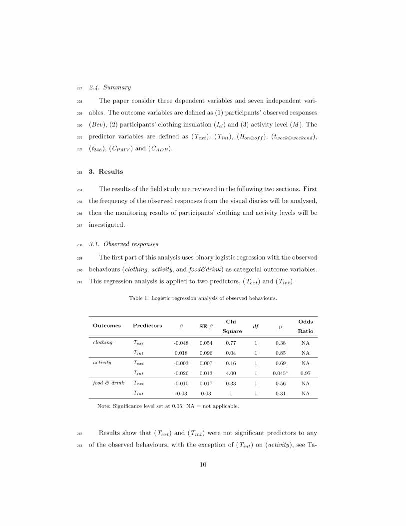
2.4. Summary227

The paper consider three dependent variables and seven independent vari-228

ables. The outcome variables are defined as (1) participants’ observed responses229

(Bev), (2) participants’ clothing insulation (Icl) and (3) activity level (M ). The230

predictor variables are defined as (Text), (Tint), (Hon⊕off ), (tweek⊕weekend),231

(t24h), (CPMV ) and (CADP ).232

3. Results233

The results of the field study are reviewed in the following two sections. First234

the frequency of the observed responses from the visual diaries will be analysed,235

then the monitoring results of participants’ clothing and activity levels will be236

investigated.237

3.1. Observed responses238

The first part of this analysis uses binary logistic regression with the observed239

behaviours (clothing, activity, and food&drink) as categorial outcome variables.240

This regression analysis is applied to two predictors, (Text) and (Tint).241

Table 1: Logistic regression analysis of observed behaviours.

Outcomes Predictors β SE βChi

Squaredf p

Odds

Ratio

clothing Text -0.048 0.054 0.77 1 0.38 NA

Tint 0.018 0.096 0.04 1 0.85 NA

activity Text -0.003 0.007 0.16 1 0.69 NA

Tint -0.026 0.013 4.00 1 0.045? 0.97

food & drink Text -0.010 0.017 0.33 1 0.56 NA

Tint -0.03 0.03 1 1 0.31 NA

Note: Significance level set at 0.05. NA = not applicable.

Results show that (Text) and (Tint) were not significant predictors to any242

of the observed behaviours, with the exception of (Tint) on (activity), see Ta-243

10

ble 1. In that case, the odds ratio was 0.97 with a 95% confidence interval of244

0.95 to 0.99. As the odds ratio was lower than 1, when (Tint) increased the245

odds of (activity) occurring decreased. This suggests that participants were246

more likely to change body position, location within a room or room when247

(Tint) decreased. Nagelkerke’s R2 of 0 indicated a very weak relationship be-248

tween the predictor (Tint) and outcome (activity) although significant. Further249

analysis reviewed the ranges and variances of (Text) and (Tint) for the three250

observed behaviours. As shown in Table 2, the ranges in (Text) and (Tint) are251

similar for the three observed behaviours. Furthermore, there is no statisti-252

cally significant difference in (Text) between observed behaviours as determined253

by one-way ANOVA (F(2,1245)=0.383, p=0.682), and there is no statistically254

significant difference in (Tint) between observed behaviours as determined by255

one-way ANOVA (F(2,1245)=0.112, p=0.894). In summary participants may256

change their clothing levels, location or food intake at similar external and in-257

ternal temperature levels.258

Table 2: Summary of the statistical characteristics of (Text) and (Tint) for the three observed

behaviours

Observed

behavioursVariables Mean σ

Mini-

mum

Maxi-

mum Range

clothing Text5.3 3.8 -2 12 14

Tint19 2.8 13.4 23 9.6

activity Text6.1 4.3 -5 15 20

Tint18.7 2.5 12.1 24.8 12.7

food & drink Text6 4.5 -3 15 18

Tint18.7 2.3 13.3 23.9 10.6

The second part of the analysis investigates the relationship between (cloth-259

ing), (activity), and (food&drink) as outcome, and (t24h) as predictor using260

11

probit regression analysis. Results summarised in Table 3 show that there261

is a significant relationship between (t24h) and both change in (clothing) and262

(food&drink) intake. However there is no significant relationship between (t24h)263

and (activity). Participants tended to change their clothing level in the morning264

(22% probability of change between 9 and 10am) and in the evening (17% prob-265

ability of change between 10 and 11pm). With regards to (food&drink) intake,266

the distribution is trimodal, with peaks at 8am, 1pm and 8pm. Both changes267

in (clothing) and (food&drink) intake may relate more to daily rhythm rather268

than responses to cold thermal discomfort.269

Table 3: Probit regression analysis of observed behaviours.

Outcomes PredictorsChi

Squaredf p

Log

likelihood

clothing t24h 35.51 21 0.025? -137.1

activity t24h 15.79 21 0.782 -4,679.9

food & drink t24h 39.89 21 0.008? -1,208.7

Note: Significance level set at 0.05.

The third part of the analysis focuses on relationship between (tweek⊕weekend),270

(Hon⊕off ), (CPMV ) and (CADP ) as predictors, and observed behaviours as out-271

comes (including ‘putting on item(s) of clothing’ (clothing), ‘changing body272

position, location within a room or room’ (activity), ‘having a warm drink, or273

food’ (food&drink)). This analysis reviews the frequencies of occurrence that274

fall into each categories. Here the outcomes and the predictors are categorical275

variables with two categories, forming 2x2 contingency tables. To alleviate the276

risk of Type I error, this analysis uses chi-square test with Yates’s continuity277

correction. The results summarised in Table 4 show that:278

• There is no significant difference in the occurrence of observed behaviours279

between weekdays and weekend day. Participants’ work patterns may280

have had an influence on this result as 45% of the participants worked281

12

full time, 35% worked part-time and 20% did not work. As a group,282

participants may have had similar patterns during weekday and weekend283

day. Further analysis showed participants were slightly more likely to be284

at home during a weekend day (57%) than a weekday (43%). To conclude285

changes in observed behaviours may be more related to daily rather than286

weekly rhythms.287

• There is no significant association between heating being on or off and288

whether or not observed behaviours occurred, with the exception of (ac-289

tivity) (χ2(1)=6.32, p<0.05). This seems to represent the fact that, based290

on the odd ratio, the odds of (activity) occurring were 0.85 (0.75, 0.97)291

times smaller if there was heating than if there was no heating.292

• There was no significant association between being within or outside of the293

three PMV categories and whether or not observed behaviours occurred,294

with the exception of (CPMV III) and (activity) (χ2(1)=5.03, p<0.05).295

This seems to represent the fact that, based on the odd ratio, the odds of296

(activity) occurring were 1.17 (1.02, 1.34) times higher if within (CPMV III)297

than if outside (CPMV III). This suggests that participants were more298

likely to change body position, location within a room or room if within299

(CPMV III).300

• There is no significant association between being within or outside of the301

three adaptive model categories and whether or not observed behaviours302

occurred.303

In summary, participants were more likely to change (activity) when there304

was no heating and when (Tint) decreased. Participants change in (clothing)305

levels and (food & drink) intake have a significant relationship with ‘time of306

day’.307

13

Table 4: Analysis of observed behaviours using chi-square test with Yates’s continuity correc-

tion.

Outcomes PredictorsSample

sizeEF

Chi

Squaredf p

Odds

Ratio

clothingtweek⊕weekend

Yes 5.53e-25 1 1 -

Hon⊕off Yes 0.02 1 0.90 -

CPMV I 2 No - - - -

CPMV II 3 No - - - -

CPMV III 4 Yes 0.07 1 0.79 -

CADP I 4 No - - - -

CADP II 4 No - - - -

CADP III 4 No - - - -

activitytweek⊕weekend

Yes 0.47 1 0.49 -

Hon⊕off Yes 6.32 1 0.012? 0.85

CPMV I 126 Yes 0.03 1 0.86 -

CPMV II 252 Yes 3.16 1 0.08 -

CPMV III 319 Yes 5.03 1 0.024? 1.17

CADP I 28 Yes 1.17 1 0.28 -

CADP II 39 Yes 1.57 1 0.21 -

CADP III 54 Yes 0.80 1 0.37 -

food & drinktweek⊕weekend

Yes 1.73 1 0.19 -

Hon⊕off Yes 0.02 1 0.88 -

CPMV I 15 Yes 3.26 1 0.07 -

CPMV II 36 Yes 1.56 1 0.21 -

CPMV III 46 Yes 1.83 1 0.18 -

CADP I 6 No - - - -

CADP II 10 No - - - -

CADP III 17 Yes 0.08 1 0.78 -

Note: Sample size, defined at the number of changes in observed behaviours that occurred within

each categories for both PMV and ADP. EF, defined as the expected frequencies greater than 5.

Significance level set at 0.05.

14

3.2. Monitored clothing insulation and activity level308

To follow the analysis of observed behaviours from the visual diary, the309

study focused on the results of the dataloggers as monitored clothing insulation310

level (Icl) and activity level (M ). In this analysis, the outcomes are defined as311

(Icl) and (M ), both are continuous and non-normally distributed variables. The312

predictors are divided into three groups, (1) (Text) and (Tint) as continuous and313

normally distributed variables, (2) (t24h) as discrete variable with 24-intervals,314

and (3) (tweek⊕weekend), (Hon⊕off ), (CPMV ) and (CADP ) as discrete variables315

with 2-categories.316

The first part of this analysis considers (Icl) and (M ) as non-normally dis-317

tributed outcome variables and investigates their relationships with (Text) and318

(Tint) using regression. In order to obtain a normally distributed sample for319

(Text) and (Tint), there is two options to transform or to ‘bootstrap’ the data.320

As the sample size is very large (>15,000), the study first identified and re-321

moved outliers for (Icl) and (M ) using z-score (significance level set at 0.05),322

and then transformed the data using square-rooting. This transformation was323

used as the size of the residuals progressively increased as values of (Text) and324

(Tint) increased. Further tests were undertook to review any fixed effect. It325

was found that participants had a significant effect on (Text) and (Tint), as326

the variations of (Text) and (Tint) between different participants were smaller327

than the variation within each participants. Post-hoc analysis using F-Test328

compared regression models with and without participants’ fixed effect, results329

show that the fixed effect models were better choices (p<0.05). The results of330

the regression analysis with participants’ fixed effect are summariesed in Table331

5.332

15

Table 5: Regression analysis of clothing (Icl) and activity (M ) level with participants’ fixed

effect.

Outcomes Predictors β SE β RF-

statisticsdf p

(Icl) Text -5e−4 4.6e−5 0.08 121 17,158 < 0.001?

Tint -2e−3 8e−5 0.18 585 17,158 < 0.001?

(M ) Text 2e−4 1e−5 0.10 363 33,660 < 0.001?

Tint -8e−5 2e−5 0.02 16 33,660 < 0.001?

Note: Significance level set at 0.05.

Results summarised in Table 5 show that (Text) and (Tint) are both signif-333

icant predictors of (Icl) and of (M ). As the coefficients are very small, a degree334

change in (Text) and (Tint) would have a small impact upon (Icl) and of (M ).335

(Text) can account for 8% of the variation in (Icl), while (Tint) can account for336

18% of the variation in (Icl). In summary participants’ clothing insulation level337

was statistically significantly influenced by both internal and external temper-338

ature. As internal and external temperature decreased, participants tended to339

increase their clothing insulation levels. With regards to activity level, results340

show that (Text) can account for 10% of the variation in (M ), while (Tint)341

can account for 2% of the variation in (M ). Participants’ activity level was sig-342

nificantly influenced by both internal and external temperatures. As internal343

temperature decreased, participants tended to increase their activity levels, al-344

though the relationship between (Tint) and (M ) is very weak.345

346

The second a part of the analysis investigates the variations of (Icl) and (M )347

throughout the day (t24h) using single factor designs ANOVA with repeated348

measures. An error term was added to reflect the fact that there is an ‘hour349

of day’ effect nested within each participants. As per the regression analysis,350

outliers were identified and removed, then (Icl) and (M ) data were transformed351

using square-rooting. Results summarised in Table 6 show that there is a sig-352

16

nificant effect of hour of the day on clothing insulation level, but there was no353

effect on activity level.354

Table 6: Analysis of the variation in clothing (Icl) and activity (M ) level throughout the day

using ANOVA.

Outcomes Predictors dfhour dfresiduals F-statistics p

(Icl) t24h 20 189 1.91 0.014?

(M ) t24h 21 237 0.93 0.55

Note: Significance level set at 0.05.

The third part of the analysis investigates the relationship between (Icl)355

and (M ) as outcome and the categorical variables (tweek⊕weekend), (Hon⊕off ),356

(CPMV ) and (CADP ) as predictors, using Mann Whitney U-test. The results357

summarised in Table 7 show that (Icl) and (M ) differ significantly between ‘Week358

day’ (Icl Mdn=0.77clo, M Mdn=1.32met) and ‘Weekend day’ (Icl Mdn=0.76clo,359

M Mdn=1.30met), although both effects are negligible and the difference in me-360

dian values are very small. This indicates that participants were significantly361

more active and were wearing more clothing during weekday. While heating362

was on, (Icl) (Mdn=0.77clo) did not differ significantly from (Icl) while heating363

was off (Mdn=0.77clo). However (M ) while heating was on (Mdn=1.35met)364

differ significantly from (M ) while heating was off (Mdn=1.29met), this effect365

and the difference in median values are small. This suggests that participants366

were statistically slightly more active when the heating was on. Metabolic rate367

increased by just under 0.1met, which is the difference between sleeping and368

reclining (ISO 8996:2004, Table B.3) [19]. With regards to PMV, results show369

that (Icl) and (M ) differ significantly between falling ‘within’ or ‘outside’ of370

the three PMV categories, with the exception of (Icl) and (CPMV III). In all371

cases the effects are small to negligible. Participants’ clothing levels were lower372

inside the PMV thresholds, whereas activity levels were higher. This may sug-373

gest that participants increased their activity rather than their clothing level to374

17

fall within the predictive comfort boundaries, although environmental variables’375

levels should also be reviewed. Finally results show that (Icl) does not differ sig-376

nificantly for (CADP ), with the exception of (Icl) and (CADP I) but in this case377

the effect is negligible. In contrast (M ) differs significantly for all (CADP ), and378

the effects are small (CADP III) to large (CADP I). Participants activity levels379

were significantly higher inside the ADP thresholds, this suggests that partici-380

pants increased their activity levels to fall within adaptive comfort boundaries.381

382

383

Table 7: Analysis of clothing and activity level using Mann Whitney U-test.

Out-

comesPredictors

Sample

size

Mdn

wk/on/in

in clo

Mdn

wd/off/out

in met

W p R

Icl tweek⊕weekend0.77 0.76 40,887,000 < 0.001? -0.03

Hon⊕off 0.77 0.77 43,053,000 0.58 <-0.01

CPMV I 4334 0.71 0.78 21,550,000 < 0.001? -0.20

CPMV II 7997 0.73 0.78 32,111,000 < 0.001? -0.16

CPMV III 10049 0.76 0.77 38,747,000 0.054 -0.01

CADP I 576 0.74 0.72 252,290 0.03? -0.06

CADP II 657 0.74 0.72 257,000 0.06 -0.05

CADP III 1109 0.74 0.71 163,960 0.43 -0.02

M tweek⊕weekend1.32 1.30 152,150,000 < 0.001? -0.02

Hon⊕off 1.35 1.29 182,210,000 < 0.001? -0.1

CPMV I 4334 1.40 1.26 45,193,000 < 0.001? <-0.01

CPMV II 7997 1.38 1.25 62,392,000 < 0.001? <-0.01

CPMV III 10049 1.37 1.26 57,762,000 < 0.001? <-0.01

CADP I 848 1.37 1.24 1,093,500 < 0.001? -0.74

CADP II 1131 1.36 1.24 1,025,000 < 0.001? -0.57

CADP III 1812 1.26 1.25 500,600 < 0.001? -0.22

Note: Sample size, defined at the number of changes in monitored behaviours that occurred within each

categories for both PMV and ADP. Mdn = Median. Significance level set at 0.05.

18

In summary, participants were most likely to increase their clothing level384

as (Tint) and (Text) decreased. Also there is a significant relationship between385

participants’ clothing level and ‘time of day’. Participants were more likely386

to wear higher clothing level during ‘week day’ than during ‘weekend day’.387

With regards to activity level, participants were likely to be active when (Tint)388

decreased, when heating was on, and during ‘week day’. Finally participants389

activity level was significantly higher while within PMV and ADP categories.390

This suggest that participants increased there activity level to fall within the391

comfort boundaries, thus ‘activity level’ may be identified as a response to392

thermal discomfort.393

4. Discussion394

4.1. Summary of the findings395

Figure 2 and Figure 3 show the significant relationships found in the six396

statistical analysis tests; the following section will compare and contrast these397

results. The observed behaviours are defined as changes in (clothing), (activ-398

ity) or (food&drink) intake; while monitored behaviours are defined as clothing399

insulation level (Icl) or activity level (M ).400

401

Both (clothing) and (Icl) have a significant relationship with time of the402

day (t24h), which may be due to daily rhythm. Reviewing variations in (cloth-403

ing) shows that there is an increase in the change of clothing in the morning404

(09:00) and evening (22:00). Reviewing variations in (Icl) shows that partici-405

pants tend to wear higher insulation level in the morning, between 06:00 and406

09:00 (Mdn=0.85 to 0.80 clo); then (Icl) decreases throughout the day to 0.6 clo407

at 01:00 in the morning. In contrast both (activity) and (M ) have no significant408

relationship with the time of the day (t24h). These results show that partici-409

pants tend to adjust their clothing level but not their activity level throughout410

the course of a day. These are interesting results and should be substantiated411

by future field studies with larger sample sizes and longer monitoring periods.412

19

Figure 2: Significant relationships between the observed behaviours and the seven predictors

reviewed in this study

Interestingly (clothing) has no significant relationship with (Tint), but (Icl)413

has a significant relationship with (Tint). Although participants did not adjust414

their clothing level while (Tint) decreased or increased, over the course of the415

study they increased their clothing level as (Tint) decreased. These results show416

that clothing may not be a direct response to a decrease in temperature, there417

might be a delay. The previous results show that variations in clothing level is418

significant throughout the course of a day, it may also be more important from419

day to day, over the course of one week or one month.420

20

Figure 3: Significant relationships between (Icl) & (M ) and the seven predictors reviewed in

this study

Both (activity) and (M ) have a significant relationship with internal temper-421

ature (Tint). As (Tint) decreased participants were more likely to change body422

position, location within the same room or room within their home. Further-423

more as (Tint) decreased participants’ activity level increased. These results424

show that participants tend to adjust their activity level with internal temper-425

ature.426

427

With regards to the other four observed behaviours, ‘turning on the heating’428

(number of observations=0), ‘closing curtains or windows’ (number of observa-429

tions=2), ‘having a warm drink, or food’ (number of observations=198), and430

‘using a hot-water-bottle or having a warm bath’(number of observations=1),431

only (food&drink) had N>30. Participants’ warm food and drink intake has a432

21

significant relationship with time of the day (t24h), but with no other predictors.433

This observed effect may be due to daily rhythm, rather than responses to ther-434

mal discomfort. In particular participants did not change their (food&drink)435

intake as internal temperature decreased. Changes in frequencies and types of436

(food&drink) intake as a response to thermal discomfort will be challenging to437

dissociate from daily rhythms and other confounding factors such as socialis-438

ing. Furthermore, it is interesting to note that participants did not interact with439

their heating systems. As mentioned in the interviews, one reason might be that440

the participants were not ‘in control’ of the heating in the household as other441

householder(s) may have been. Another reason might be that the participants442

did not want to interfere with the settings of the system. Having estimated443

when the heating was on or off (Hon⊕off ) for each participants, the review of444

the profiles shows dwellings with short on-off heating cycles which are most445

likely to be associated with constant heating and thermostatic control; while446

others show longer on-off heating cycles. In some cases these appear regular,447

suggesting programmed timers, in other dweillings they are more random and448

therefore more likely to be associated with manual control. The state of heating449

(on or off) was a signifiant predictor to change in (activity) and activity level450

(M ). When the heating was off, participants increased their changes of activity,451

but reduced their activity level overall (from Mdn=1.35 met with the heating452

on to Mdn=1.29 met with the heating off). One reason might be that partic-453

ipants may be more static (i.e. sitting) and may change their body position454

more frequently (i.e. putting their hands under their legs or ‘crouching down’).455

456

The current thermal comfort models rely on people’s reported thermal sen-457

sations, rather than people responses to thermal discomfort. These models as-458

sume that if outside their set categories people should feel ‘uncomfortable’ and459

therefore act upon their state of discomfort. However the results of this study460

show that there is no relationship between observed behaviours and (CPMV )461

& (CADP ); with the exception of (activity) and (CPMV III). Participants were462

more likely to change body position, location within a room or room to fall463

22

within (CPMV III). In contrast the results show that there are significant rela-464

tionships between monitored behaviours and (CPMV ) & (CADP ). Participants465

were more likely to increase there activity and clothing levels to fall within466

(CPMV ), furthermore participants were more likely to increase there activity467

level to fall within (CADP ). In summary (CPMV ) & (CADP ) did not lead to a468

change in observed behaviours but lead to increased activity and clothing levels.469

To remain comfortable, participants retain higher activity and clothing levels.470

The methods employed in this paper enabled people’s behaviours to be explored471

within these standard categories.472

4.2. Summary of the statistical analysis methods473

This study uses a mix of parametric and non-parametric tests to analyse474

the field study’s data. The data were treated as numeric including the catego-475

rial variables, i.e. observed behaviours and predictors (tweek⊕weekend, Hon⊕off ,476

CPMV and CADP ) represented as discrete and binary data. A common pro-477

cedure was undertaken to assigned values to these categorial variables. For478

example, if an observed behaviour occurred the value ‘1’ was assigned, else it479

was assigned the value ‘0’; a similar process was undertaken for the predictors480

tweek⊕weekend, Hon⊕off , CPMV and CADP . (t24h) was represented as a discrete481

and interval variable. Finally (Icl), (M ), (Text) and (Tint) were represented482

as continuous variables. The normality of the continuous data was assessed,483

as (Icl) and (M ) were non-normally distributed a square-root function was ap-484

plied. Having determined the class of the outcomes and predictors, statistical485

tests were applied for each combination of variables, summarised as follows:486

• (Outcomes, Observed behaviours, Discrete binary) with (Predictors, (Text)487

and (Tint), Continuous): Logistic regression488

• (Outcomes, Observed behaviours, Discrete binary) with (Predictors, (t24h),489

Discrete interval): Probit regression490

• (Outcomes, Observed behaviours, Discrete binary) with (Predictors, (t24h),491

Discrete binary): Chi-square test with Yates’s continuity correction492

23

• (Outcomes, (Icl) and (M ), Continuous normally distributed) with (Pre-493

dictors, (Text) and (Tint), Continuous): Ordinary least squares regression494

with fixed effect495

• (Outcomes, (Icl) and (M ), Continuous normally distributed) with (Pre-496

dictors, (t24h), Discrete interval) Repeated measure ANOVA497

• (Outcomes, (Icl) and (M ), Continuous not normally distributed) with498

(Predictors, (t24h), Discrete binary) Mann Whitney U-test499

These analyses investigated the probability of behavioural responses to cold500

thermal discomfort in particular the significances and trends between variables.501

4.3. Interval and external validity502

The study employs a range of sensors to collect information, and each device503

may introduce measurement errors. To address this bias, it is import to review504

the accuracy and to test the precision of each sensor. For the environmen-505

tal equipment, calibration tests were undertaken in climate chamber; results506

were compared to standard benchmarks [24]. Further bias might have been507

introduced by the positioning of sensors, in particular the height at which the508

environmental sensors were positioned. Consequently future studies may deploy509

a greater number of environmental sensors. With regards to the SenseCam, the510

main limitations of this method are the cost of the device, storage capacity and511

battery life. The study relied on four SenseCams, that were handed-out to four512

participants at a time. Participants were ask to recharged the device every two513

days overnight, as fully charged battery corresponds to 12 hours of operation514

[25]. With regards to storage capacity, the SenseCam could store over 20,000515

pictures [25]. As an average of 7,300 pictures were taken for each participants516

over 10-days, future studies may extend the monitoring period. Another limi-517

tation of this method might be that participants may forget to wear the device.518

Having reviewed the frequency of usage and asked the participants during the519

final interviews if they had forgotten to wear the SenseCam, this only occurred520

in few instances. One reason might be that is was winter. If the participant521

24

was to go-out, the SenseCam should be taken off just before leaving the home,522

and placed near the entrance door or on the coat-stand. When returning home,523

the SenseCam should be worn again. The advice was ‘coat on - SenseCam off’,524

and ‘coat off - SenseCam on’. If a similar study was conducted in the summer525

the frequency of ’wear’ might differ. Finally further bias may be introduced526

by the ‘observer effect’. To follow the results of the feedback interviews, the527

first monitoring day was not taken into account in the analysis. Although most528

participants reported feeling less self-conscious of wearing the SenseCam after529

the first few hours, the potential Hawthorne effect may continue throughout the530

monitoring study. Future studies may look at developing a similar device than531

the SenseCam but without the in-built camera.532

533

The participants taking part in the main study were related to the University,534

and therefore they may have similar attitudes and lifestyles. Future studies may535

look at recruiting participants from an established subject pool. The research536

was set in people’s home. This environment may allow for greater adaptive537

opportunities than non-domestic buildings. If a study was to be carried out in538

office setting, then a similar framework may be applied. The set of wearable539

sensors may not include a camera for privacy concerns, yet additional factors540

may be monitored; for example operational power of computer or lighting may541

enable participants’ location and activity to be ascertained. The dwellings were542

all located in the South East of England, therefore participants may apply sim-543

ilar local adaptation responses. Future studies may be carried out in different544

regions or climate where responses may be influenced by specific geographical545

and cultural features. The framework develop in this study may then be used546

to investigate variations in local adaptation. Finally, the results of this study547

rely on the observed and monitored behaviours of twenty participants, there-548

fore these results cannot be extrapolated to a population, a much larger and549

representative sample should be employed for this purpose. Nevertheless the550

methods developed to collect and analyse objective data may be deployed in551

future studies investigating occupants’ behaviours.552

25

5. Conclusions553

5.1. New insights554

The paper reviewed the variability of behavioural responses to cold thermal555

discomfort as a function of environmental, temporal and standard factors. Key556

findings include the following:557

• The change and level in activity increased as internal temperature de-558

creased. This may add to the formulation of models which include be-559

haviour adaptation, as described by Schweiker and Wagner [29].560

• Clothing thermal adaptation may not occur as an immediate response to561

changes in internal temperature, but as a delayed response. Future studies562

may be carried out over longer period of time to investigate these potential563

variations in clothing level.564

5.2. Implications565

Methodologically, this research establishes an empirical study design to in-566

vestigate the probability of behavioural responses to thermal discomfort. Fur-567

thermore it demonstrates the efficacy of different statistical tools to predict the568

probability of occupants’ behaviours to adapt to thermal discomfort.569

6. Acknowledgements570

This work was supported by the UK Engineering and Physical Sciences Re-571

search Council under Grant EP/H009612/1.572

References573

[1] Matthew Lipson, Smart Systems and Heat. Consumer challenges for low574

carbon heat, Tech. rep., Energy Technologies Institute, Loughborough, UK575

(2015).576

26

[2] Majcen, D., Itard, L. and Visscher, H., Statistical model of the heating pre-577

diction gap in Dutch dwellings: Relative importance of building, household578

and behavioural characteristics, Energy and Buildings 105 (2015) 43–59.579

[3] Yan, D., O’Brien, W., Hong, T., Feng, X., Gunay, H. B., Tahmasebid, F.580

and Mahdavi, A., Occupant behavior modeling for building performance581

simulation: Current state and future challenges, Energy and Buildings 107582

(2015) 264–278.583

[4] Rupp, R. F., Vasquez, N. G. and Lamberts, R., A review of human thermal584

comfort in the built environment, Energy and Buildings 105 (2015) 178–585

205.586

[5] Sonderegger, R. C., Movers and Stayers: The Resident’s Contribution to587

Variation Across Houses in Energy Consumption for Space Heating, Savin588

Energy in the Home. Princeton’s Experiments at Twin Rivers. (Ed. So-589

colow, R. H.) Chapter 9 (1978) 207–230.590

[6] Heerwagen, J. and Diamond, R., Adaptations and Coping: Occupant Re-591

sponse to Discomfort in Energy Efficient Buildings, Proceedings of 1992592

Summer Study on Energy Efficiency in Buildings 10 (1992) 83–90.593

[7] Brager, G. and de Dear, R., Thermal adaptation in the built environment:594

a literature review, Energy and Buildings 27 (1998) 83–96.595

[8] Karjalainen, S., Thermal comfort and use of thermostats in Finnish homes596

and offices, Building and Environment 44 (2009) 1237–1245.597

[9] Hwang, R. and Chen, C., Field study on behaviors and adaptation of elderly598

people and their thermal comfort requirements in residential environments,599

Indoor Air 20 (2010) 235–245.600

[10] Tweed, C., et al., Thermal comfort practices in the home and their impact601

on energy consumption,, Architectural Engineering and Design Manage-602

ment 10(1-2) (2014) 1–24.603

27

[11] Burris, A., Mitchell, V. and Haines, V., Exploring Comfort in the Home:604

Towards an Interdisciplinary. Framework for Domestic Comfort, Proceed-605

ings of the NCEUB conference 2012 - ‘The changing context of comfort in606

an unpredictable world’, Windsor, UK.607

[12] Bolger, N., Davis, A. and Rafaeli, E., Diary Methods: Capturing Life as it608

is Lived, Annu. Rev. Psychol. 54 (2003) 579–616.609

[13] Sellen, A. et al., Do life-logging technologies support memory for the past?610

An experimental study using SenseCam, Proceedings of the SIGCHI Con-611

ference on Human Factors in Computing Systems, New York USA (2007)612

81–90.613

[14] Pink, S., Situating everyday life: practices and places, Sage, London, UK,614

2012.615

[15] Hitchings, R. and Day, R., How older people relate to the private winter616

warmth practices of their peers and why we should be interested, Environ-617

ment and Planning 43 (2011) 2457–2467.618

[16] International Organization for Standardization (ISO), BS EN ISO619

7730:2005: Ergonomics of the thermal environment - Analytical deter-620

mination and interpretation of thermal comfort using calculation of the621

PMV and PPD indices and local thermal comfort criteria, Tech. rep., ISO,622

Geneva, Switzerland (2005).623

[17] Wunderground, Weather History for London City, United Kingdom,624

http://www.wunderground.com/ (Access date: 2015-09-30), 2015.625

[18] Chartered Institution of Building Services Engineers (CIBSE), Degree-626

days: theory and application. TM41: 2006, Tech. rep., London, UK (2006).627

[19] International Organization for Standardization (ISO), BS EN ISO628

8996:2004 Ergonomics of the thermal environment - Determination of629

metabolic rate, Tech. rep., ISO, Geneva, Switzerland (2004).630

28

[20] S. Gauthier, D. Shipworth, Predictive thermal comfort model: are current631

field studies measuring the most influential variables?, Conference proceed-632

ings: 7th Windsor Conference: The Changing Context of Comfort in an633

Unpredictable World. NCEUB, London, UK. (2012) 1–14.634

[21] Department for Communities and Local Government (DCLG), English635

Housing Survey Questionnaire Documentation, Year 4 (2011/12), Tech.636

rep., UK (2012).637

[22] International Organization for Standardization (ISO), BS EN ISO638

10551:2001: Ergonomics of the thermal environment - Assessment of the639

influence of the thermal environment using subjective judgement scales,640

Tech. rep., ISO, Geneva, Switzerland (2001).641

[23] Hong, S. et al., A field study of thermal comfort in low-income dwellings642

in England before and after energy efficient refurbishment, Building and643

Environment 44 (2009) 1228–1236.644

[24] International Organization for Standardization (ISO), BS EN ISO645

7726:2001 Ergonomics of the thermal environment - Instruments for mea-646

suring physical quantities, Tech. rep., ISO, Geneva, Switzerland (2001).647

[25] Hodges, S. et al., SenseCam: A Retrospective Memory Aid, Proceedings648

of UbiComp 8th International Conference on Ubiquitous Computing 4206649

(2006) 177–193.650

[26] S. Gauthier, D. Shipworth, Behavioural responses to cold thermal discom-651

fort, Building Research & Information 43:3 (2015) 355–370.652

[27] CEN, Standard BS EN 15251, Indoor environmental input parameters for653

design and assessment of energy performance of buildings addressing in-654

door air quality, thermal environment, lighting and acoustics, Tech. rep.,655

European Committee for Standardisation, Brussels, Belgium (2007).656

29

[28] Huebner, G. et al., Heating patterns in English homes: Comparing results657

from a national survey against common model assumptions, Building and658

Environment 70 (2013) 298–305.659

[29] Schweiker, M. and Wagner, A., A framework for an adaptive thermal heat660

balance model (ATHB), Building and Environment 94 (2015) 252–262.661

30

Due  to  ethical  restrictions,  supporting  data  cannot  be  made  openly  available.