investigating the quality of modeled aerosol profiles based on

Investigating the quality of modeled aerosol profiles based oncombined lidar and sunphotometer dataNikolaos Siomos1, Dimitris S. Balis1, Anastasia Poupkou1, Natalia Liora1, Spyridon Dimopoulos1,Dimitris Melas1, Eleni Giannakaki2,5, Maria Filioglou1,2, Sara Basart3, and Anatoli Chaikovsky4

1Laboratory of atmospheric physics, Physics Department, Aristotle University of Thessaloniki, Greece2Finnish Meteorological Institute, Atmospheric Research Centre of Eastern Finland, Kuopio, Finland3Earth Sciences Department, Barcelona Supercomputing Center, BSC-CNS, Barcelona, Spain4Institute of Physics, National Academy of Science, Minsk, Belarus5Department of Environmental Physics and Meteorology, Faculty of Physics, University of Athens, Greece

Correspondence to: N. Siomos ([email protected])

Abstract. In this study we present an evaluation of the Comprehensive Air Quality Model with extensions CAMx for Thes-

saloniki using radiometric and lidar data. The aerosol mass concentration profiles of CAMx are compared against the fine and

coarse mode aerosol concentration profiles retrieved by the Lidar-Radiometer Inversion Code LIRIC. The CAMx model and

the LIRIC algorithm results were compared in terms of mean mass concentration profiles, center of mass and integrated mass

concentration in the boundary layer and the free troposphere. The mean mass concentration comparison resulted in profiles5

within the same order of magnitude and similar vertical structure for the fine particles. The mean center of mass values are

also close with a fractional bias of 24.8%. On the opposite side, the coarse mode appears to be underestimated by the model

below 4km and overestimated above. In order to grasp the reasons behind the discrepancies, we investigate the effect of aerosol

components that are not properly included in the model’s emission inventory and boundary conditions such as the wildfires

and the desert dust component. The identification of the cases that are affected by wildfires is performed using wind backward10

trajectories from the Hybrid Single Particle Lagrangian Integrated Trajectory Model HYSPLIT in conjunction with satellite

fire pixel data from the MODerate-resolution Imaging Spectroradiometer (MODIS) Terra and Aqua global monthly fire loca-

tion product MCD14ML. By removing those cases the correlation coefficient improves from 0.44 to 0.86 for the fine mode

integrated mass in the boundary layer. The fine mode center of mass fractional bias also decreases to 16.9%. Concerning the

analysis on the desert dust component, the simulations from the updated version of the former Dust Regional Atmospheric15

Model called BSC-DREAM8b were deployed. When only the desert dust cases are taken into account, BSC-DREAM8b gen-

erally outperforms CAMx when compared with LIRIC, achieving a correlation of 0.91 and a fractional bias of -18.9% for

the integrated mass in the free troposphere and a correlation of 0.44 for the center of mass. CAMx, on the other hand, both

underestimates and anti-correlates the integrated mass in the free troposphere. Consequently, the accuracy of CAMx is limited

concerning the transported dust cases. We conclude that the performance of CAMx appears to be best for the fine particles,20

especially in the boundary layer. At the same time it systematically fails to successfully predict the coarse mode. Sources of

particles not properly taken into account by the model are confirmed to negatively affect its performance.

1

Atmos. Chem. Phys. Discuss., doi:10.5194/acp-2016-1125, 2017Manuscript under review for journal Atmos. Chem. Phys.Published: 13 January 2017c© Author(s) 2017. CC-BY 3.0 License.

1 Introduction

There is a wide variety of atmospheric models that are capable of providing vertical profiles of the aerosol mass concentration

(e.g. CAMx, BSC-DREAM8b, European Monitoring and Evaluation Programme EMEP, LOng Term Ozone Simulation -

EURopean Operational Smog model LOTOS-EUROS, CHIMERE). This is achieved through simulation of the atmospheric

motion and the chemical reactions that are taking place inside the atmosphere. The most common approach to validate the5

modeled vertical mass concentration products is to compare with surface and columnar concentration or optical measurements

either from ground-based or satellite instruments (e.g., Takemura et al., 2002; Stier et al., 2005; Katragkou et al., 2010; Huneeus

et al., 2011; Basart et al., 2012a; Marécal et al., 2015). This approach, however, doesn’t verify the ability of the model to

accurately predict the vertical distribution of the aerosol concentration. Observational aerosol profiles comparable with the

modeled ones are required for this purpose. Remote sensing techniques such as lidar measurements can provide us with this10

sort of profiles. Since the main lidar products typically involve optical aerosol properties such as the aerosol backscatter and

extinction coefficient profiles, it is common to ensure comparability by converting the model’s output after applying appropriate

techniques. For example Mona et al. (2014) compare between the dust extinction profiles of the BSC-DREAM8b model and

the respective EARLINET (European Aerosol Research LIdar NETwork) profiles for a 12 year period in Potenza. Meier et al.

(2012) use lidar backscatter profiles as one of the tools to evaluate the Consortium for Small-scale Modeling - Multi-Scale15

Chemistry Aerosol Transport (COSMO-MUSCAT) model for the PM2.5 and PM10 particles. Hodzic et al. (2004) recreate the

lidar attenuated backscatter profiles using the output of the CHIMERE model in order to compare the model’s PM10 profiles

with the lidar measurements.

On the other hand, there are techniques that allow the estimation of the aerosol vertical concentration from remote sensing

lidar measurements using a suitable algorithmic inversion method (e.g., Böckmann, 2001; Veselovskii et al., 2002; Raut and20

Chazette, 2009; Lopatin et al., 2013; Chaikovsky et al., 2016). The advantage of this approach is that the modeled product

can be directly validated without the need of conversion. The literature focused on the validation of dust transportation mod-

els with observational aerosol concentration profiles is quite mature. For example, Binietoglou et al. (2015) have presented

a methodology based on LIRIC to evaluate the performance of dust models using data from multiple AERONET (AErosol

RObotic NETwork) and EARLINET stations. Granados-Muñoz et al. (2016) also use the LIRIC algorithm to compare be-25

tween observational data and a variety of dust models in the frame of July 2012 CHemistry and AeRosols Mediterranean

EXperiments ChArMEx/EMEP campaign. However, there is a lack of studies that focus on the evaluation of both PM2.5 and

PM10 concentration profiles simulated by atmospheric models. Royer et al. (2011) compare the simulations of the CHIMERE

chemistry transport model for the PM10 particles using lidar PM10 concentration profiles derived with the methodology of

Raut and Chazette (2009). In this study we investigate the validity of the aerosol concentration profiles simulated with the30

air quality model Comprehensive Air Quality Model with extensions (CAMxversion5.3), (ENVIRON 2010, 2010) for Thes-

saloniki, Greece (40.5N, 22.9E) using the results of the Lidar/Radiometer Inversion Code (LIRIC). Instead of evaluating the

performance of CAMx only for the PM10 particles, we separate the fine from the coarse aerosols and perform the validation

for each mode individually.

2


CAMx is running operationally to produce a 3-day air quality forecast for Thessaloniki (Zyryanov et al., 2012; Marécal

et al., 2015). It provides vertical concentration profiles of a variety of gaseous and aerosol components.

A second model, the desert dust transportation model BSC-DREAM8b (Nickovic et al., 2001; Pérez et al., 2006a, b; Basart

et al., 2012b) has also been included in the analysis in order to investigate the performance of CAMx in the case of dust

transportation events. This model can provide total dust concentration profiles.5

The LIRIC inversion (Chaikovsky et al., 2016), on the other hand, is a technique used to estimate the concentration profiles of

the fine and coarse mode aerosol using both sunphotometer and lidar data. Lidar and sunphotometer measurements performed

at the Laboratory of Atmospheric Physics of the Aristotle University of Thessaloniki, Greece (40.5N, 22.9E) from the period

2013-2015 were used as input data for the algorithm.

Validating the accuracy of CAMx simulations for Thessaloniki for the period 2013-2015 could prove useful in the aerosol10

classification procedure of the lidar measurements since individual aerosol components are provided by CAMx. Furthermore,

from the modelers’ point of view, the comparison could also reveal the need of adjustments in the model’s aerosol emissions,

boundary conditions and mixing processes.

The paper is organized as follows. In section 2 the two models, CAMx and BSC-DREAM8b, and the LIRIC algorithm are

described in detail. The 3rd section is devoted to the methodology of the analysis. This includes the preprocessing of the lidar15

and the sunphotometer measurements and the characterization of the lidar profiles, the demonstration of the strategy that we

applied for the comparison and the application of two example cases. The results of the study are discussed in section 4. Finally,

section 5 contains the main conclusions of this study.

2 Data, Algorithm and Models

2.1 The lidar system of Thessaloniki20

Lidar measurements from the THEssaloniki LIdar SYSstem (THELISYS), that is located at the Laboratory of Atmospheric

Physics (LAP) of the Aristotle University of Thessaloniki (40.5o N, 22.9o E) at 50m above sea level, during the period 2013-

2015 were selected for this study. The setup of the system in this period includes two raman channels at 355nm and 532nm

and three elastic channels at 355, 532 and 1064nm. The raw lidar signals from the elastic channels at the three aforementioned

wavelengths are necessary in order to perform the LIRIC inversion. All signal pre-prepossessing procedures are applied di-25

rectly in the LIRIC algorithm. The lidar station of Thessaloniki participates in the European Aerosol Research Lidar Network

(EARLINET) Schneider et al. (2000) since 2000. More details on the instrument can be found in Amiridis et al. (2005) and

(Giannakaki et al., 2010).

2.2 The CIMEL sunphotometer

In order to apply the LIRIC inversion, sunphotometer observations are necessary. The CIMEL multiband sun-sky photometer30

of Thesaloniki was deployed for this purpose. The instrument participates in the AERONET Global Network. It belongs to the

3


Laboratory of Atmospheric Physics (LAP) and it is located in a distance less than 50m from the lidar instrument (see section

2.1) in the same altitude. It automatically performs direct solar irradiance and sky radiance measurements at 340, 380, 440, 500,

670, 870, and 1020nm. The data processing is performed automatically with the AERONET inversion algorithms (Dubovik

and King, 2000; Dubovik et al., 2006). The level 2 Version 2 Inversion data during the period 2013-2015 were used in this

study. The instrument and the AERONET infrastructure are described in detail in Holben et al. (1998).5

2.3 The Comprehensive Air quality Model with extensions CAMx

An air quality forecast modeling system was set-up in the framework of the EU Monitoring Atmospheric Composition and

Climate (MACC) project. It consists of the meteorological model Weather Research and Forecasting model (WRF version

3.5.1) described in Skamarock et al. (2008) and the photochemical model CAMx (version 5.3). It is designed to provide the air

quality forecast in four nested grids covering Europe (30 km spatial resolution European grid covering also a part of Sahara10

desert), the Eastern Mediterranean (10 km spatial resolution grid) and the Greek urban centers Thessaloniki and Athens (2 km

spatial resolution grids). A nesting technique is applied in order to increase the accuracy at the area of interest i.e. Thessaloniki.

A single grid point in Thessaloniki is chosen at (40.633 N, 22.956 E) for the model outputs processed in the present study to

coincide with the lidar measurements. The model grids are configured in 17 vertical layers extending up to about 9.5 km above

ground level (agl). The temporal resolution of CAMx outputs and consequently of the simulated profiles is one hour.15

The aerosol particles are modeled using a static two-mode coarse/fine scheme in CAMx for the representation of the particle

size distribution. Fine particles have an aerodynamic diameter smaller than 2.5 µm while coarse particles have an aerodynamic

diameter higher than 2.5 µm and smaller than 10 µm. A total of 20 individual aerosol components plus the aerosol water content

that is absorbed by the hygroscopic particles are provided by the model (see table 1). The aerosol aqueous inorganic chemistry

is applied according to the RADM-AQ aqueous chemistry algorithm (Chang et al., 1987). The partitioning of the inorganic20

aerosol constituents between the gas and aerosol phases is performed using the ISORROPIA thermodynamic module (Nenes

et al., 1998). The secondary organic aerosol (SOA) formation/partitioning was performed with the use of the SOAP scheme

(Strader et al., 1999). SOA are formed by non-methane volatile organic compounds of anthropogenic and natural origin. Details

on the CAMx aerosol components such as the hygroscopicity and the fine or coarse mode type can be found in table 1.

CAMx is applied with the use of gaseous and particulate anthropogenic and natural emissions. Particulate matter emissions25

from natural sources (windblown dust and sea salt aerosol) and biogenic volatile organic compounds from vegetation are es-

timated using the Natural Emission MOdel NEMO version 1 (Markakis et al., 2009; Poupkou et al., 2010; Markakis, 2010)

driven by the WRF meteorology. The Model for the Spatial and Temporal Distribution of Emissions (MOSESS) (Markakis

et al., 2013) was applied for the calculation of spatially and temporally disaggregated and chemically speciated anthropogenic

emission data of the following pollutants: CO, NOx, SO2, NH3, NMVOC, PM10 and PM2.5. The anthropogenic emissions30

were estimated using either activity data with methodologies and emission factors of the EMEP/CORINAIR - CORe INven-

tory AIR emission inventory guidebook (EEA, 2006) or the emission database of The Netherlands Organization (TNO) for

the reference year 2007 (Kuenen et al., 2011). Anthropogenic emissions for the following sources are accounted for: energy

production, central heating, industry, transportation, waste treatment and disposal, agricultural activities (i.e. biomass burning,

4


fertilization), extraction and distribution of fossil fuels. It is important to mention that particle emissions due to dust resus-

pension from agricultural activities and road traffic as well as the wildfire emissions are not currently included in CAMx

simulations. Saharan dust emissions are taken into account only indirectly in the CAMx chemical boundary conditions pro-

vided by the global forecast modeling systems Integrated Forecasting System IFS-MOZART until October 2014 and C-IFS

afterwards (Flemming et al., 2009; Morcrette et al., 2009; Stein et al., 2012) in the framework of the MACC project. The model5

has been evaluated during the MACC-II project (Marécal et al., 2015) and also with observations from the National Monitoring

Network of the Air Quality (Melas et al., 2017).

2.4 The BSC-DREAM8b model

The transported desert dust particles and the forest fire particles are common categories of aerosol components in Thessaloniki

(Amiridis et al., 2005; Basart et al., 2009; Giannakaki et al., 2010). As it has already been stated, the setup of CAMx in10

Thessaloniki includes the desert dust component only from the global boundary conditions and it doesn’t include wildfire

emissions at all. Biases in those two aerosol components are expected to affect both aerosol modes since the desert dust

particles are coarse dominant (Shettle and Fenn, 1979; d’Almeida, 1987) and the biomass burning particles are fine dominant

(Tesche et al., 2009; Groß et al., 2013).

The desert dust component can be further analyzed by comparing LIRIC with a dust specialized model. The dust transporta-15

tion model BSC-DREAM8b (Pérez et al., 2006a, b; Nickovic et al., 2012; Basart et al., 2012b) was chosen for the comparison.

BSC-DREAM8b is managed by the Barcelona Supercomputer Center (BSC) and provides operational forecasts since May

2009, and is also participating in the northern Africa–MiddleEast–Europe (NA-ME-E) node of the World Meteorological Or-

ganization (WMO) Sand and Dust Storm Advisory and Assessment System (SDS-WAS) project. The BSC-DREAM8b model

is embedded into the Eta/NCEP atmospheric model and solves the mass balance equation for dust, taking into account the20

different processes of the dust cycle (i.e., dust emission, transport and deposition). The updated version of the model includes

8 particle size bins (0.1–10 µm radius range) and dust-radiative feedback.

The BSC-DREAM8b model has been evaluated for longer periods over northern Africa and Europe (e.g., Jiménez-Guerrero

et al., 2008; Pay et al., 2010; Pay et al., 2012; Basart et al., 2012b, a; Gama et al., 2015) and against experimental campaigns

in source regions during the SAharan Mineral dUst experiMent SAMUM-1 (Haustein et al., 2009) and the Bodélé Dust Ex-25

periments (BoDEx, Todd et al., 2008). Furthermore, daily evaluation of BSC-DREAM8b with near-real-time observations is

conducted at BSC. Currently, the daily operational model evaluation includes satellites (MODIS and MSG - Meteosat Second

Generation) and AERONET sun photometers. Some comparisons between lidar and forecast models profiles were performed

in terms of aerosol vertical distribution for specific Saharan dust events in the Mediterranean Basin (e.g., Balis et al., 2004;

Pérez et al., 2006a; Amiridis et al., 2009; Mona et al., 2012; Gobbi et al., 2013; Amiridis et al., 2013; Mona et al., 2014). In30

addition, Binietoglou et al. (2015) includes BSC-DREAM8b as one of the models that participate in their analysis validating

its performance against LIRIC retrievals in 10 EARLINET/AERONET stations.

The present analysis includes the daily runs of BSC-DREAM8b. The initial state of dust concentration in the model was

defined by the 24 h forecast from the previous-day model run. The Final Analyses of the National Centers of Environment

5


Prediction (NCEP/FNL; at 1o×1o) at 0UTC were used every 24 hours as initial conditions and boundary conditions at intervals

of 6h. The model configuration used for the present study includes 24 Eta vertical layers extending up to approximately 15 km

in the vertical. The resolution is set to 0.3o in the horizontal. The temporal resolution of the simulations is 3 h. The domain of

simulation covers northern Africa, the Middle East and Europe. It is worth mentioning that re-suspended wind-blown dust and

the considered desert dust sources are limited to northern Africa and the Middle East (< 35o N) in the BSC-DREAM8b model.5

2.5 The LIdar-Radiometer Inversion Code LIRIC

The LIRIC algorithm utilizes both radiometric data that have been processed by the AERONET inversion algorithm (Dubovik

and King, 2000; Dubovik et al., 2006) and also raw lidar signals at three wavelengths (355 nm, 532 nm and 1064 nm) in order

to estimate the aerosol concentration profiles for the fine and coarse particles. The radiometric data used as input includes

the aerosol size distribution, the aerosol volume concentration in the two modes (fine and coarse), the aerosol optical depth10

(AOD) and the single scattering albedo (SSA) of each mode, the complex refractive index in each wavelength, the sphericity

and the aerosol phase function. The minimum of the aerosol size distribution in the 0.194 - 0.576 µm radius range is used as

the size boundary that separates the fine from the coarse mode. In case that the particle depolarization ratio is also provided, it

is possible for the algorithm to further separate the spherical coarse particles from the non spherical ones. Nevertheless, only

the fine and coarse mode retrievals are taking part in this study due to the lack of depolarization ratio profiles.15

The algorithm main products are the vertical volume concentration profiles in the two modes. In brief, the algorithm searches

for the profile per mode that gives the best agreement between the actual data and the reconstructed data from the algorithm, also

demanding a certain degree of vertical smoothness in the final product. The reconstructed data include the aerosol backscatter

profiles in the three lidar wavelengths and the columnar volume concentration values per mode. A detailed description of LIRIC

can be found in Chaikovsky et al. (2016).20

The effects of multiple user defined uncertainties on the final result has been studied by Granados-Muñoz et al. (2014)

while Filioglou et al. (2016) present a sensitivity study of the effect of the algorithm’s input parameters to the final profiles.

Furthermore, the LIRIC retrievals have already been evaluated for volcanic and desert dust particles by Wagner et al. (2013)

showing that the inversion can be accurate for two quite different types of aerosol. The aerosol extinction products of LIRIC

has also been compared against the respective products from the Generalized Aerosol Retrieval from Radiometer and Lidar25

Combined data (GARRLiC) algorithm and against the retrievals from raman lidar measurements (Bovchaliuk et al., 2016).

3 Methodology

The analysis is divided in two parts. Section 3.1 corresponds to the preprocessing of the algorithm’s and the model’s estimates

in order to calculate comparable final products. The characterization procedure of the lidar profiles is also described there. The

methodology of the comparison is included in section 3.2. Two sample cases are presented in section 3.3 aiming to give an30

example of the products that the algorithm and the models can provide and also to demonstrate typical problems that occur in

the analysis.

6


3.1 Preprocessing

In the first part of this section, the preprocessing procedure of the lidar measurements is described. In the second part, we

present the methodology that was applied in order to characterize the lidar profiles.

3.1.1 Lidar preprocessing

The LIRIC algorithm requires both the raw lidar signal resulting from the atmospheric elastic backscattering in 355nm, 532nm5

and 1064nm and the Version 2 Inversions from AERONET. Lidar measurements performed in Thessaloniki during the period

2013-2015 were used for this purpose. Before September 2012, the setup of the lidar system in Thessaloniki was lacking

a 1064nm channel that is necessary for the LIRIC inversion. A manual cloud screening process was also applied in order

to remove all the cloud affected lidar measurements since LIRIC is not designed for cloud layers. In addition, only daytime

measurements were used since the sunphotometer only operates during daytime. It is important to mention that both instruments10

are located close to one another and at the same altitude above sea level (see section 2.1 and section 2.2).

The sunphotometer data are processed by the AERONET algorithms in order to calculate the necessary aerosol properties

which are required as input for the algorithm. In our analysis, the closest AERONET inversion to the central time of the lidar

measurement was selected for the LIRIC retrievals. Cases with an absolute time difference that exceeded 3 hours between the

sunphotometer measurement time and the central time of the lidar measurement were excluded. The lidar signal preprocessing15

is performed directly in LIRIC (Chaikovsky et al., 2016) and includes the averaging, smoothing, background correction and

range correction procedures as well as the normalization of the lidar signals and also the selection of the lower and upper height

boundaries in the signal where the LIRIC inversion is going to be performed. All the signals are adjusted to a common vertical

resolution with a constant step of 15m. A lower height boundary has to be determined due to the overlap function of the lidar

system. In the current dataset the full overlap height was calculated at 900m. The lower boundary is set to 600m where the20

overlap function is still above 90%. Below this height the lidar signals are considered constant. As it was mention in section

2.3, this can produce uncertainties since the radiometric data corresponds to the whole atmospheric column and most of the

aerosol are usually located in the boundary layer, close to the ground. According to Granados-Muñoz et al. (2014) the selection

of the lower limit is the main source of error. They estimate the maximum uncertainty due to such intrinsic errors at 33%

and the overall profile error to stay below 15% most of the time. The upper boundary depends on the maximum height where25

aerosol exist in a significant quantity and can vary depending on the atmospheric conditions. The output data of the algorithm

includes vertical volume concentration profiles of the fine and coarse mode particles in ppbv. By summing the concentration

in the two modes one can calculate the total aerosol concentration.

The vertical resolution of the LIRIC products and the model products is different so it was necessary to upscale LIRIC to the

resolution of each model. This can affect the vertical structure of the profiles for individual cases but in a statistical analysis30

those effects will be smoothed (Binietoglou et al., 2015). The temporal resolution of CAMx forecasts is one hour while the

temporal resolution of BSC-DREAM8b forecasts is three hours. Each of the retrieval algorithm’s profiles were matched to the

models’ profile closest to the central lidar measurement. Since LIRIC derived concentration values are in ppbv units while

7


both models’ profiles are in µg ·m−3 units, it was necessary to apply a unit conversion that also requires the aerosol density.

Despite the aerosol component densities of CAMx being known, we preferred to convert ppbv to µg ·m−3 (equation 1) since

µg ·m−3 is more widely used as a concentration unit.

cµg·m−3 = 103 · cppbv · ρg·cm−3 (1)

Where ρ is the mean aerosol density. Typical density values of 1.5 and 2.6 g · cm−3 for the fine and coarse mode particles were5

used respectively (Bukowiecki et al., 2011; Schumann et al., 2011; Kokkalis et al., 2013).

3.1.2 Characterization of the lidar profiles

It was mentioned in section 2.3 that the emission inventory of CAMx lacks the biomass burning aerosol emissions from

wildfires. Additionally, the desert dust emissions are taken into account only indirectly in the CAMx chemical boundary

conditions (section 2.3). In order to examine the effect of those cases on the comparison we group the cases in four categories.10

The first one is the total of the cases that will be refer to as ’all’. The second one contains the cases identified as biomass burning

wildfire aerosol and will be referred to as "fires" from now on. The aerosol characterization is performed using a combination

of model simulations and satellite data. It is described in the next paragraph. When the category ’fires’ is screened from the

category ’all’, the category ’non fires’ is formed. It contains the continental and desert dust cases. Finally, the desert dust cases

are also isolated and are included in the category ’dust’.15

The backward trajectories from HYSPLIT in conjunction with fire pixel data from the MODIS Terra and Aqua Global

Monthly Fire Location Product (MCD14ML) are used to identify the fire cases. The dust cases characterization also utilizes

the HYSPLIT trajectories in combination with the BSC-DREAM8b profiles. A pair of 6-day back-trajectories, one arriving in

the boundary layer region and another in the Free Troposphere, were used. The technique that was utilized in order to estimate

the boundary layer height per case is described in section 3.2. A high fire spot density on a region where the air masses are20

passing near ground is applied as a criterion for the wildfire cases identification.

The trajectories for the continental, desert dust and biomass burning cases are presented in figure 1 with blue (a and b),

orange (c and d) and black color (e and f) respectively. The left column contains the air masses that arrive in the boundary

layer, typically around 1km while the right column the ones that arrive in the Free Troposphere, usually ranging between 3 and

4km. Each trajectory is accompanied by the corresponding accumulated 6-day fire pixels.25

3.2 Comparison Strategy

The first part of the evaluation of CAMx is based on the comparison of the aerosol concentration with the LIRIC estimates for

the ’all’ category (section 4.1). The effect of the wildfire cases on the results is also examined in this section. In the second

part, the accuracy of CAMx in events of transported Saharan dust is investigated (section 4.2).

The concentration profiles of all the fine aerosol components (table 1) are summed to create the fine mode concentration30

profile of CAMx. The same applies to the coarse aerosol components of table 1. The water content is included in the fine mode

since all the hygroscopic particles are fine.

8


The number of cases that take part in the comparison as well as the high variability between individual cases emphasize

the need of statistics in the analysis. The mean profiles of the two models and LIRIC are calculated across the vertical range.

The center of mass is also calculated for each case and each mode. It provides additional information on the height where the

majority of the particles are located.

The Planetary boundary layer (PBL) marks the top of the layer where the atmosphere is well mixed and the local aerosol5

component is also expected to be significant. On the other hand, the Free Troposphere (FT) above, is related to much less

mixing and a stronger transported aerosol component is expected. Consequently, a comparison between CAMx and LIRIC in

the boundary layer and in the free troposphere would be useful in order to investigate the accuracy of the model in these quite

different atmospheric regions. Thus, we calculate the fine and coarse integrated mass in the boundary layer and in the Free

Troposphere for each case.10

There are multiple techniques in order to estimate the boundary layer from lidar measurements (e.g., Flamant et al., 1997;

Menut et al., 1999; Brooks, 2003). Baars et al. (2008) apply a wavelet covariance transform on the lidar range-corrected signal

in order to translate signal layers to maxima and minima of the Wavelet Covariance Transform (WCT). Here we apply the

transform to the total concentration derived by LIRIC. However this is not enough to automatically identify the PBL since the

boundaries of multiple layers will be retrieved. Identification criteria are necessary for the selection of the PBL height. The15

top of the layer between 400m and 2.5km with the minimum value in the transformed signal is chosen as the boundary layer

height. The wavelet transform is applied to the LIRIC concentration profiles before the upscaling of the resolution.

To perform the integration below and above the PBL a lower and an upper boundary is required. The LIRIC inversion

requires a height where the aerosol content is not significant. This height is usually different for each case and typically ranges

between 3km and 9km. On the other hand, CAMx always provides values up to 9.5km while BSC-DREAM8b provides values20

up to 15km. We used the ground level as the common lower boundary and the upper limit of CAMx (9.5km) as the common

upper boundary. Since LIRIC profiles usually end below this upper limit, the last value of each profile is considered constant

up to 9.5km.

Metrics for the center of mass and the integrated mass in the boundary layer and in the Free Troposphere are also calculated.

This includes the mean values and the standard deviations for the algorithm and the model, the mean bias error, the mean25

fractional error the root mean square error (RMSE), the correlation coefficient and the least squares fit slope and axis intersect

values. The equations for some of the metrics can be found on table 2.

In order to demonstrate how the comparison strategy was applied we present two distinct cases which includes the aerosol

typing procedure, the concentration profiles comparison and the optical products that can be derived by the LIRIC algorithm.

3.3 Example Cases30

The products of LIRIC, CAMx, BSC-DREAM8b and HYSPLIT for 2 case studies are presented here.

The main product of LIRIC is the fine and coarse mode concentration profiles. Additionally, the aerosol extinction and

backscattering efficiencies per mode and per wavelength (355nm, 532nm, 1064nm) are also derived. The total extinction and

backscatter coefficient profiles, symboled as a and b respectively, for the three wavelengths are calculated using the equations

9


2 and 3, were Qext is the extinction efficiency and Qbsc is the backscattering efficiency. The concentration for the fine and

coarse mode is marked as cf and cc respectively.

a(λ,z) =Qext,f (λ) · cf (z) +Qext,c(λ) · cc(z) (2)

b(λ,z) =Qbsc,f (λ) · cf (z) +Qbsc,c(λ) · cc(z) (3)5

Then, from the LIRIC estimated extinction and backscatter profiles, the lidar ratio and the angstrom exponent can also be

calculated. Furthermore, as it was mentioned in section 3.1, the concentration values below 600m are kept constant in the

LIRIC inversion and this also applies to the optical products.

A typical continental case on the 13th of January 2014 and a typical dust case on the 27th of August 2013 were selected in

order to demonstrate the comparison results for two quite different typical aerosol types. The continental case is demonstrated10

on the left of figure 2 and the Saharan dust case on the right column.

The trajectories indicate a continental case on 13th of January 2014. They are presented in figure 2a. Additionally there

could be some mixing with marine particles from the Adriatic sea. The air mass arriving in the free troposphere should be

clean according to HYSPLIT since the trajectory is elevated, always above 3km. The concentration profiles of LIRIC and

CAMx are presented in figure 2c and figure 2d. According to LIRIC the fine mode is dominant below 1km. Above that height15

there is a coarse dominant layer which could be the result of mixing with marine aerosol. The fine mode aerosol concentration

profile of CAMx seems in good agreement with LIRIC in the near range, below 2km. On the other hand, CAMx fails to predict

the coarse mode. Above 6km, an overestimation of CAMx can be observed in both profiles.

The four optical products are also presented. The upper part of figure 2g panel contains the aerosol backscatter and extinction

coefficient profiles and the lower part the lidar ratio and the Angstrom exponent profiles. The lidar ratio values are around 7020

sr−1 at 355nm and 65 sr−1 at 532nm below 1km. The Angstrom values are near 1.6 for the 355-532nm exponent and at 2.1

for the 532-1064nm exponent. Giannakaki et al. (2010) report a mean lidar ratio at 355nm of 56 ± 23 sr−1 and a backscatter-

related Angstrom exponent at 355-532nm of 1.4 ± 1.0 for the continental polluted aerosol class in Thessaloniki. Between

1km and 2km the lidar ratio at 355nm drops to 55 sr−1 and the lidar ratio 532nm at 45 sr−1. The Angstrom exponent in both

regions drops near 1.3. According to Giannakaki et al. (2010) those values are still within the range of the acceptable range of25

the continental polluted class.

As far as the second case is considered, the trajectories indicate an event of transported Saharan dust in the FT (figure 2b).

The air masses that arrive in the PBL seem to contain marine aerosol from the Mediterranean, probably mixed with emissions

from local urban sources. A strong coarse mode can be observed in figure 2e both for the layer below 1.5km and the layer

above. Despite CAMx predicting a promising fine mode (figure 2d), it fails to do so for the coarse particles. This is the reason30

why the BSC-DREAM8b concentration profile is presented here instead. This model describes the dust layer between 2km and

5km much better. Below 2km the model isn’t compatible any more with the observation.

As far as the optical products are concerned, the lidar ratio at 355nm and 532nm values range between 40 and 50 sr−1 for

the whole profiles while the Angstrom exponent ranges between 1.0 and 1.5 for both spectral regions (figure 2h). Giannakaki

10


et al. (2010) calculate a lidar ratio at 355nm of 52 ± 18 sr−1 and a backscatter-related Angstrom exponent at 355-532nm of

1.5 ± 1.0 for the Saharan dust aerosol class at Thessaloniki which seems compatible with this case. In the next section the

statistical analysis is presented and the results are discussed.

4 Discussion

An ensemble of 24 measurements, that fulfill the criteria described in section 3.2, took part in this comparison. These cases5

constitute the category ’all’. In the first part of this section (section 4.1) the comparison between LIRIC and CAMx is presented.

In the second part (section 4.2) the accuracy of CAMx in case of Saharan dust events is investigated using the simulations of

BSC-DREAM8b.

4.1 Comparison between LIRIC and CAMx

In this section the simulated profiles of CAMx are compared against the observational profiles of LIRIC. The vertical mean10

profiles derived from LIRIC and CAMx for the fine and coarse mode particles are displayed in figure 3a and figure 3b. The

solid lines correspond to the ’all’ category, while the dashed lines correspond to the ’no fires’ category, which consists of

17 measurements. It can be seen that the fine mode mean concentration profiles show a good agreement between LIRIC and

CAMx. The vertical structure also seems to bear some similarities. There is an overall slight overestimation by the model which

becomes more significant above 2km. Removing the 7 wildfire cases modifies the LIRIC mean profile towards slightly lower15

values and the CAMx mean profile towards slightly higher values, leading to smaller discrepancies below 1km. Details on the

behavior of the model in the boundary layer and the free troposphere for both the ’all’ and the ’no fires’ categories can be found

in the next paragraphs. As far as the coarse mode is considered, it seems to be severely underestimated by the model especially

below 3km. Above 4.5km the model seems to overestimate the aerosol concentration. The reasons of these discrepancies could

be connected with the model’s emissions inventory and the boundary conditions. Some insight can be offered by individually20

inspecting the contribution of each aerosol component in the final product.

The mean concentration profiles of the aerosol components that consist the fine and coarse mode of CAMx are presented in

figure 3c and figure 3d. The aerosol components of table 1 are grouped into categories that follow the OPAC formalism (Hess

et al., 1998). The Particulate Chloride and Sodium components form the "sea salt" category. The Aerosol Water Content, the

Primary Elemental Carbon, the Fine Crustal and Coarse Crustal as well as the Fine Other Primary and Coarse Other Primary25

components are independent and form the categories "water", "soot", "soil fine", "soil coarse", "other fine" and "other coarse"

respectively. The particulate Nitrate, the Sulfate and the particulate Ammonium are all hygroscopic and are grouped into the

"water soluble" category. The rest of the species are all organic and are grouped in the "organic insoluble" category. The Fine

Other Primary component contains the fine particles that are considered as inert by the model as well as a part of the fine sea salt

that cannot be categorized neither as Particulate Chloride nor as Sodium. The Coarse Other Primary component contains the30

coarse particles that take part in chemical reactions like nitrate, sulfate, ammoniac, black carbon and primary organic aerosol,

as well as the coarse sea salt and all the other coarse particles that are considered as inert by the model.

11


The dominant component below 2km is the water soluble one, followed by the fine sea salt component and the water content.

Above 2km the other fine component becomes significantly stronger with a maximum at 3-4km. This region matches with the

one where CAMx overestimates the fine mode. Consequently, the "other fine" component could be connected to these biases.

As far as the coarse mode is considered, the majority of particles belong to the soil coarse component. Both components seem

responsible for the overestimation above 4km in the coarse mean profiles since the highest values in both both component5

profiles are located above 2km. In order to investigate if only one of them or both are also responsible for the large bias below

3km we isolate the dust component by selecting only the dust cases. This comparison is presented in section 4.2. Below, the

center of mass and the integrated mass are calculated in order to further quantify the comparison results.

The center of mass (table 2) provides information on the height where most of the particles are located. It is presented in

LIRIC against CAMx center of mass scatter plots (figure 4) for the fine and the coarse mode. The least squares fit line and10

the correlation coefficient for the ’no fires’ category is displayed in the plots. A synopsis of the center of mass metrics can be

seen in table 3. The ’no fires’ category is not included for the coarse aerosol. LIRIC estimates a mean center of mass value

of 1.06 ± 0.23 km for the "all" category which increases slightly for the "no fires" category in the fine mode. CAMx predicts

a mean center of mass at 1.36 ± 0.47 km that doesn’t change much if the wildfire cases are excluded. Thus, the resulting

mean bias is 0.30 km and the fractional bias is 24.8% and they improve to 0.20km and 16.9% respectively. The root mean15

square error (RMSE) stays constant near 0.55km. Consequently, the height where most of the fine particles are located seems

well-predicted by the model. As far as the coarse mode is considered, LIRIC gives a mean value of 1.36 ± 0.60 km while

CAMx predicts the center of mass at 3.16 ± 1.21 km. As a result, the mean bias and the RMSE are much larger here, which

is expected given the large discrepancies that were discussed in the previous paragraph. The correlation coefficient for the fine

mode is 0.20 and increases to 0.34 when the wildfire cases are excluded. While the center of mass is useful when examining20

the vertical distribution and the location of the maximum concentration, it doesn’t provide any insight on the concentration

itself. Additional information on the accumulated concentration within an atmospheric region can be provided by calculating

the integrated mass.

The comparison of the integrated mass in the boundary layer and the free troposphere is displayed in LIRIC against CAMx

integrated mass scatterplots (figure 5) and the metrics are presented in table 4. The coarse mode isn’t included since it seems25

to be significantly biased by the model.

The behavior of the model in the boundary layer is examined first. LIRIC estimates a mean integrated mass at 18.8 ± 16.0

mg ·m−2 against a CAMx derived value of 14.1 ± 10.5 mg ·m−2 for the "all" category which change to 14.1 ± 8.6 mg ·m−2

and 16.1 ± 10.5 mg ·m−2 respectively for the "no fires" category. The mean bias changes from -4.7 mg ·m−2 to 2.0 mg ·m−2

that translates to a fractional bias shift from -28.6 to 13.2%. The RMSE improves from 14.7 mg ·m−2 to 6.1 mg ·m−2. The30

correlation coefficient is at 0.44 and the least square fit slope at 0.29 for the "all" category but they both improve to 0.81 and

0.99 respectively when the wildfire cases are removed. The results that occur for the "no fires" category indicate that, in the

boundary layer, the lack of wildfire emissions in CAMx shouldn’t be neglected as it obviously affect the performance of the

model.

12


The behavior of the model in the free troposphere is quite different. The LIRIC mean value is 18.8 ± 16.0 mg ·m−2 against

a CAMx mean value of 14.1 ± 10.5 mg ·m−2. By excluding the wild fire cases the LIRIC mean stays almost the same, at 23.1

± 18.4 mg ·m−2 but the CAMx mean increases to 32.5 ± 31.9 mg ·m−2. This causes the mean bias and RMSE to actually

increase from 8.1 mg ·m−2 and 33.3 mg ·m−2 to 16.6 mg ·m−2 and 35.6 mg ·m−2 respectively. The fractional bias is also

negatively affected and increases from 28.5 to 53.2%. On the other hand, the correlation coefficient is at 0.25 and the least5

square fit slope at 0.45 for the "all" category and they improve to 0.36 and 0.69 respectively for the "no fires" category. All

things considered, the removal of the wildfire cases doesn’t seem to positively affect the agreement between the CAMx and

LIRIC in the free troposphere. This is also depicted in the scatterplot (figure 5, on the right) where the "fires" cases (red) are

all quite close to the unity line in contrast with the boundary layer (figure 5, on the left) where most of those cases seem to be

outliers. Discrepancies in the free troposphere could also be attributed to the fact that the LIRIC profile above the height where10

the aerosol load is insignificant is considered constant (see sections 3.1.1 and 3.2) while the CAMx profile is still active in that

region. Additionally, a possible preference of the biomass burning layers to arrive in the PBL over Thessaloniki could also be

associated with this behavior.

Taking into account the performance of CAMx in both atmospheric regions, it appears to predict the fine aerosol more accu-

rately in the boundary layer than in the free troposphere. This behavior seems consistent with the previous results considering15

that CAMx tends to estimate higher concentration values in higher altitudes (figure 3 and figure 4) in the fine mode, which

could also be attributed to the "other fine" component. When the wildfire cases are not taken into account the performance of

the model improves but only in the PBL. Possible causes for the discrepancies between LIRIC and CAMx could be the aerosol

emission inventory of CAMx and the chemical boundary conditions. We have shown here that cases that also include wildfire

aerosols are a challenge for the model since those emissions are not included at all. It has been stated in section 2 that the soil20

dust resuspension emissions are also not included and that the Saharan dust emissions are included indirectly. The large dis-

crepancies in the coarse mode mean profile could be connected to a combination of the lack of dust resuspension emissions and

of biased Saharan dust boundary conditions. In the next section the behavior of CAMx in transported dust events is analyzed.

4.2 Dust cases analysis using BSC-DREAM8b

In this section the coarse mode products derived by LIRIC are compared against the simulations of both CAMx and BSC-25

DREAM8b. Out of the initial dataset of 24 measurements, 6 were identified as dust cases. We have to mention that the focus of

this study is not a validation of BSC-DREAM8b since the number of dust cases wouldn’t be sufficient. The BSC-DREAM8b

model is used here solely to support the analysis of CAMx. That being said, we aim to isolate the coarse desert dust component

and compare between LIRIC and each model in order to investigate if the observed large discrepancies in the coarse mode of

CAMx are also present in the simulations of a model that specializes in desert dust. While it is feasible to get the coarse dust30

profile with CAMx from the coarse profile by selecting only the "soil coarse" component (table 1) this is not the case for the

coarse profile of LIRIC. Having applied the aerosol characterization of section 3.1.2, it is reasonable to assume that the coarse

mode of the selected dust cases is almost entirely attributed to dust. Binietoglou et al. (2015) also use a dataset of measurements

that were flagged as desert dust in order to compare between the observations and the simulations of the dust transportation

13


models. Obtaining the coarse dust of BSC-DREAM8b is also not an option because this model provides total dust profiles.

d’Almeida (1987) mention that the contribution of the fine dust should be low, especially near where is emitted. Mamouri and

Ansmann (2014) have separated the fine and coarse mode dust profiles during an outbreak event. They report that while the

fine dust contribution in the mass concentration was significant near the ground in that transported dust case, it stayed well

below 20% of the total concentration above 400m. Consequently, the use of the total dust profile of BSC-DREAM8b shouldn’t5

jeopardize much the validity of the comparison with LIRIC, especially in the free troposphere.

The mean profiles of the aerosol mass concentration in the coarse mode is presented in figure 6. The comparison between

CAMx and LIRIC can be seen on the left while the comparison between BSC-DREAM8b and LIRIC is presented on the right.

It is obvious that CAMx underestimates the concentration by providing values that never exceed 10 µg ·m−3 while the LIRIC

mean values raise up to 45 µg ·m−3 and potentially much higher for selective cases. On the other hand, BSC-DREAM8b10

values are close to the ones derived by LIRIC between 2km and 4km, ranging between 20 and 40 µg ·m−3. Below 2km, even

BSC-DREAM8b seems to underestimate the concentration. This could be attributed to mixing with coarse particles other than

desert dust in this region. This scenario is further supported by taking into account the "dust" category trajectories that arrive

in the PBL (figure 1c) in section 3.3. In the next paragraphs the center of mass and the integrated mass comparison is presented

in a way similar to section 4.1.15

The center of mass comparison between LIRIC and BSC-DREAM8b is presented in figure 7a accompanied by the observa-

tional and modeled metrics in table 5. CAMx predicts a center of mass at 2.55 ± 1.13 km which is actually close to the value of

BSC-DREAM8b at 2.38 ± 0.57. Discrepancies in the mean bias here originate mainly from differences in the LIRIC center of

mass product that occur due to differences from the interpolation of the LIRIC profile to the vertical resolution of each model.

The correlation coefficient and the least square fit slope values are at -0.13 and -0.28 respectively between the algorithm and20

the air quality model but they improve at 0.44 and 0.39 when the dust transportation model is used instead. Binietoglou et al.

(2015) estimate a correlation coefficient of 0.38 for the same model and for a dataset of 69 dust profiles.

As far as the integrated mass is considered, the comparison of LIRIC vs BSC-DREAM8b is also presented in figure 7, the

boundary layer in figure 7b and the free tropospheric region in figure 7c. The agreement is best in the free tropospheric region

for the dust specialized model which is in accordance with the profiles of figure 6. The mean values for BSC-DREAM8b in25

the FT are 90.1 ± 94.9 mg ·m−2. They are quite close to the mean values of LIRIC at 108.9 ± 72.9 mg ·m−2 resulting to

the lowest absolute mean bias of table 6 at -18.8 mg ·m−2 and a fractional error of -18.9%. The respective fractional error of

CAMx in the FT is -103.3% . The correlation between LIRIC and BSC-DREAM8b in the same region is high, at 0.91, and the

least square fit slope is 1.19 in contrast with the PBL region where the slope is much lower at 0.23 despite the correlation being

similar. Binietoglou et al. (2015) report a correlation of 0.54 for the integrated dust concentration in the whole profile for their30

dataset of 69 measurements. As it has already been mentioned, discrepancies between the algorithm and the models can occur

from the non dust aerosol component. This can be crucial for the PBL region, where particles from various sources are mixed.

The comparison between LIRIC and the two models resulted to a much better performance of BSC-DREAM8b than CAMx

in the free troposphere for the dust cases. The dust specialized model was able to reproduce values similar to the observations,

leading to the conclusion that the "soil coarse" component of CAMx is definitely underestimated. This behavior could be linked35

14


to the model’s lack of direct Saharan dust emissions within the domain (see section 2.3). Having said that, the desert dust cases

are not the majority and by removing the 6 dust cases out of the 24 total cases didn’t improve much the coarse profile of CAMx.

In order to explain these large biases (section 4.1) we have to assume that the "other coarse" component is also biased, most

probably underestimated below 4km. This component contains the coarse sea salt and also the coarse ammoniac, sulfate and

nitrate particles (see table 1 and section 4.1) that are all supposed to be hygroscopic. Despite that, the "other coarse" component5

is not treated as hygroscopic by the model. Thus the water absorption and the hygroscopic growth of the coarse particles is

not taken into account at all. Consequently, the absence of any water content in the coarse mode of CAMx could lead to an

underestimation of the model since LIRIC concentration profiles include the water content absorbed by the fine and coarse

particles.

5 Conclusions10

The evaluation of CAMx resulted in a mean profile in the same order of magnitude and of similar vertical distribution with

the observational one for the fine mode. The mean center of mass of the model is different by only 0.3km from the respective

value of the algorithm which translates to a mean fractional bias of 24.8%. The correlation coefficient is estimated at 0.20 and

improves at 0.34 when the wildfires are excluded. The integrated mass comparison indicates a better performance of the model

in the boundary layer than in the free troposphere. For the "no fires" category, the mean fractional bias improves from -28.6 to15

13.2%. At the same time, the correlation coefficient of the integrated mass rises from 0.44 to 0.86 and the least squares fit slope

from 0.29 to 0.99. The comparison in the free tropospheric region, on the other hand, is not clearly benefited from the removal

of those cases. All things considered, there are strong indications that the lack of the wildfire emissions in CAMx affect it’s

performance concerning the mass concentration of the fine mode particles that arrive in the boundary layer.

The coarse mode mean profile of CAMx, on the other hand seems to be greatly underestimated below 4km and overestimated20

above. Consequently, the vertical structure is also incompatible with the observational data. The behavior of the "soil coarse"

component of CAMx was tested using selected dust cases and the desert dust dispersion model BSC-DREAM8b. Both models

underestimate the concentration in the boundary layer. In the free troposphere, BSC-DREAM8b achieves a fractional bias of

-18.9% and a correlation coefficient at 0.91 in contrast with CAMx where the same metrics are estimated at -103.3% and

-0.69 respectively. The center of mass is also better correlated in the dust model. Care has to be taken, however, because the25

interpolation of the LIRIC profiles in the models’ vertical resolution affects the center of mass and shifts the LIRIC mean

value by from 1.75km for the resolution of CAMx to 2.14km for the resolution of BSC-DREAM8b. Since BSC-DREAM8b

outperforms CAMx, at least in the free troposphere, it is reasonable to assume that the "soil coarse" component is a source of

bias. Furthermore, the fact that the small number of the dust cases (6 out of 24) is not enough to explain the large discrepancies

in the coarse mode mode between LIRIC and CAMx, it is likely that the "other coarse" component is also biased. This could30

be linked to the fact that it consists of many subcomponents, some of which in theory are hygroscopic, like the coarse sea salt,

but they are not treated as such by the model, possibly leading to underestimations in the aerosol concentration.

15


This study shows that the LIRIC code, based on the synergy of and lidar measurements can be used in order to evaluate

an air quality model like CAMx as far as the aerosol mass concentration is considered. Furthermore, models specialized in

particular types of emissions, like the BSC-DREAM8b dust transportation model, can be used along with LIRIC in order to

help isolate one specific aerosol component that the air quality models provides or completely lacks. That way, the components

can be tested individually, making it possible to directly associate biases with a specific type of emissions. Here, for example,5

we concluded that the lack of a wildfire component, the desert dust component and the remaining coarse component are all

potential sources of bias in the modeled aerosol concentration profiles. The emissions that are associated with these aerosol

types can then be examined and proper corrections could be applied in order to improve the overall performance of the model.

Finally, if such comparisons are successful then the simulations of the model can also be utilized in the aerosol classification

procedure of the lidar measurements since the individual aerosol components of the model could provide insight on the origin10

of the main aerosol layers.

Acknowledgements. The authors would like to acknowledge the EU projects MACC-III (Monitoring Atmospheric Composition and Climate

- III, Grant agreement no: 633080) and MACC-II project (Monitoring Atmospheric Composition and Climate - Interim Implementation,

Grant agreement no: 283576). The simulated results presented in this research paper have been produced using the EGI and HellasGrid

infrastructures. The ACTRIS-2 project from the European Union’s Horizon 2020 research and innovation programme under grant agreement15

No 654109 is gratefully acknowledged. The authors would also like to acknowledge the support provided by the Scientific Computing Center

at the Aristotle University of Thessaloniki throughout the progress of the work on air quality forecasting. BSC-DREAM8b simulations were

performed on the Mare Nostrum supercomputer hosted by Barcelona Supercomputing Center-Centro Nacional de Supercomputación (BSC-

CNS). S. Basart wants to acknowledge the CICYT project (CGL2013-46736). Elina Giannakaki acknowledges the support of the Academy

of Finland (project no. 270108).20

16


References

Amiridis, V., Balis, D. S., Kazadzis, S., Bais, A., Giannakaki, E., Papayannis, A., and Zerefos, C.: Four-year aerosol observations with a Ra-

man lidar at Thessaloniki, Greece, in the framework of European Aerosol Research Lidar Network (EARLINET), Journal of Geophysical

Research: Atmospheres, 110, n/a–n/a, doi:10.1029/2005JD006190, http://dx.doi.org/10.1029/2005JD006190, d21203, 2005.

Amiridis, V., Kafatos, M., Perez, C., Kazadzis, S., Gerasopoulos, E., Mamouri, R. E., Papayannis, A., Kokkalis, P., Giannakaki, E., Basart,5

S., Daglis, I., and Zerefos, C.: The potential of the synergistic use of passive and active remote sensing measurements for the validation

of a regional dust model, Annales Geophysicae, 27, 3155–3164, doi:10.5194/angeo-27-3155-2009, http://www.ann-geophys.net/27/3155/

2009/, 2009.

Amiridis, V., Wandinger, U., Marinou, E., Giannakaki, E., Tsekeri, A., Basart, S., Kazadzis, S., Gkikas, A., Taylor, M., Baldasano, J., and

Ansmann, A.: Optimizing CALIPSO Saharan dust retrievals, Atmospheric Chemistry and Physics, 13, 12 089–12 106, doi:10.5194/acp-10

13-12089-2013, http://www.atmos-chem-phys.net/13/12089/2013/, 2013.

Baars, H., Ansmann, A., Engelmann, R., and Althausen, D.: Continuous monitoring of the boundary-layer top with lidar, Atmospheric

Chemistry and Physics, 8, 7281–7296, doi:10.5194/acp-8-7281-2008, http://www.atmos-chem-phys.net/8/7281/2008/, 2008.

Balis, D. S., Amiridis, V., Nickovic, S., Papayannis, A., and Zerefos, C.: Optical properties of Saharan dust layers as detected by a Ra-

man lidar at Thessaloniki, Greece, Geophysical Research Letters, 31, n/a–n/a, doi:10.1029/2004GL019881, http://dx.doi.org/10.1029/15

2004GL019881, l13104, 2004.

Basart, S., Pérez, C., Cuevas, E., Baldasano, J. M., and Gobbi, G. P.: Aerosol characterization in Northern Africa, Northeastern Atlantic,

mediterranean basin and middle east from direct-sun AERONET observations, Atmospheric Chemistry and Physics, 9, 8265–8282, www.

scopus.com, 2009.

Basart, S., Pay, M. T., Jorba, O., Pérez, C., Jiménez-Guerrero, P., Schulz, M., and Baldasano, J. M.: Aerosols in the CALIOPE air quality20

modelling system: evaluation and analysis of PM levels, optical depths and chemical composition over Europe, Atmospheric Chemistry

and Physics, 12, 3363–3392, doi:10.5194/acp-12-3363-2012, http://www.atmos-chem-phys.net/12/3363/2012/, 2012a.

Basart, S., Pérez, C., Nickovic, S., Cuevas, E., and Baldasano, J.: Development and evaluation of the BSC-DREAM8b dust regional model

over Northern Africa, the Mediterranean and the Middle East, Tellus B, 64, http://www.tellusb.net/index.php/tellusb/article/view/18539,

2012b.25

Binietoglou, I., Basart, S., Alados-Arboledas, L., Amiridis, V., Argyrouli, A., Baars, H., Baldasano, J. M., Balis, D., Belegante, L., Bravo-

Aranda, J. A., Burlizzi, P., Carrasco, V., Chaikovsky, A., Comerón, A., D’Amico, G., Filioglou, M., Granados-Muñoz, M. J., Guerrero-

Rascado, J. L., Ilic, L., Kokkalis, P., Maurizi, A., Mona, L., Monti, F., Muñoz Porcar, C., Nicolae, D., Papayannis, A., Pappalardo, G.,

Pejanovic, G., Pereira, S. N., Perrone, M. R., Pietruczuk, A., Posyniak, M., Rocadenbosch, F., Rodríguez-Gómez, A., Sicard, M., Siomos,

N., Szkop, A., Terradellas, E., Tsekeri, A., Vukovic, A., Wandinger, U., and Wagner, J.: A methodology for investigating dust model30

performance using synergistic EARLINET/AERONET dust concentration retrievals, Atmospheric Measurement Techniques, 8, 3577–

3600, doi:10.5194/amt-8-3577-2015, http://www.atmos-meas-tech.net/8/3577/2015/, 2015.

Böckmann, C.: Hybrid regularization method for the ill-posed inversion of multiwavelength lidar data in the retrieval of aerosol size distri-

butions, Appl. Opt., 40, 1329–1342, doi:10.1364/AO.40.001329, http://ao.osa.org/abstract.cfm?URI=ao-40-9-1329, 2001.

Bovchaliuk, V., Goloub, P., Podvin, T., Veselovskii, I., Tanre, D., Chaikovsky, A., Dubovik, O., Mortier, A., Lopatin, A., Korenskiy, M.,35

and Victori, S.: Comparison of aerosol properties retrieved using GARRLiC, LIRIC, and Raman algorithms applied to multi-wavelength

17


lidar and sun/sky-photometer data, Atmospheric Measurement Techniques, 9, 3391–3405, doi:10.5194/amt-9-3391-2016, http://www.

atmos-meas-tech.net/9/3391/2016/, 2016.

Brooks, I. M.: Finding Boundary Layer Top: Application of a Wavelet Covariance Transform to Lidar Backscatter Profiles, Journal of

Atmospheric and Oceanic Technology, 20, 1092–1105, doi:10.1175/1520-0426(2003)020<1092:FBLTAO>2.0.CO;2, http://dx.doi.org/

10.1175/1520-0426(2003)020<1092:FBLTAO>2.0.CO;2, 2003.5

Bukowiecki, N., Zieger, P., Weingartner, E., Jurányi, Z., Gysel, M., Neininger, B., Schneider, B., Hueglin, C., Ulrich, A., Wichser, A., Henne,

S., Brunner, D., Kaegi, R., Schwikowski, M., Tobler, L., Wienhold, F. G., Engel, I., Buchmann, B., Peter, T., and Baltensperger, U.: Ground-

based and airborne in-situ measurements of the Eyjafjallajökull volcanic aerosol plume in Switzerland in spring 2010, Atmospheric

Chemistry and Physics, 11, 10 011–10 030, doi:10.5194/acp-11-10011-2011, http://www.atmos-chem-phys.net/11/10011/2011/, 2011.

Chaikovsky, A., Dubovik, O., Holben, B., Bril, A., Goloub, P., Tanré, D., Pappalardo, G., Wandinger, U., Chaikovskaya, L., Denisov,10

S., Grudo, J., Lopatin, A., Karol, Y., Lapyonok, T., Amiridis, V., Ansmann, A., Apituley, A., Allados-Arboledas, L., Binietoglou, I.,

Boselli, A., D’Amico, G., Freudenthaler, V., Giles, D., Granados-Muñoz, M. J., Kokkalis, P., Nicolae, D., Oshchepkov, S., Papayan-

nis, A., Perrone, M. R., Pietruczuk, A., Rocadenbosch, F., Sicard, M., Slutsker, I., Talianu, C., De Tomasi, F., Tsekeri, A., Wagner, J.,

and Wang, X.: Lidar-Radiometer Inversion Code (LIRIC) for the retrieval of vertical aerosol properties from combined lidar/radiometer

data: development and distribution in EARLINET, Atmospheric Measurement Techniques, 9, 1181–1205, doi:10.5194/amt-9-1181-2016,15

http://www.atmos-meas-tech.net/9/1181/2016/, 2016.

Chang, J. S., Brost, R. A., Isaksen, I. S. A., Madronich, S., Middleton, P., Stockwell, W. R., and Walcek, C. J.: A three-dimensional

Eulerian acid deposition model: Physical concepts and formulation, Journal of Geophysical Research: Atmospheres, 92, 14,

doi:10.1029/JD092iD12p14681, 1987.

d’Almeida, G. A.: On the variability of desert aerosol radiative characteristics, Journal of Geophysical Research: Atmospheres, 92, 3017–20

3026, doi:10.1029/JD092iD03p03017, http://dx.doi.org/10.1029/JD092iD03p03017, 1987.

Dubovik, O. and King, M. D.: A flexible inversion algorithm for retrieval of aerosol optical properties from Sun and sky radiance mea-

surements, Journal of Geophysical Research: Atmospheres, 105, 20 673–20 696, doi:10.1029/2000JD900282, http://dx.doi.org/10.1029/

2000JD900282, 2000.

Dubovik, O., Sinyuk, A., Lapyonok, T., Holben, B. N., Mishchenko, M., Yang, P., Eck, T. F., Volten, H., Muñoz, O., Veihelmann, B., van der25

Zande, W. J., Leon, J.-F., Sorokin, M., and Slutsker, I.: Application of spheroid models to account for aerosol particle nonsphericity in

remote sensing of desert dust, Journal of Geophysical Research: Atmospheres, 111, n/a–n/a, doi:10.1029/2005JD006619, http://dx.doi.

org/10.1029/2005JD006619, d11208, 2006.

EEA: EMEP/CORINAIR Emission Inventory Guidebook - 2006., Tech. Rep. 11/2006., European Environmental Agency, 2006.

ENVIRON 2010: User’s Guide CAMx Comprehensive Air Quality Model with Extensions., Version 5.30, ENVIRON International Corpo-30

ration, 2010.

Filioglou, M., Siomos, N., Poupkou, A., S., D., Chaikovsky, A., and Balis, D. S.: A sensitivity study of the LIdar-Radiometer Inversion Code

(LIRIC) using selected cases from Thessaloniki database, International Journal of Remote Sensing, the article is currently under review,

2016.

Flamant, C., Pelon, J., Flamant, P. H., and Durand, P.: Lidar determination of the entrainment zone thickness at the top of the unstable marine35

atmospheric boundary layer, Boundary-Layer Meteorology, 83, 247–284, doi:10.1023/A:1000258318944, http://dx.doi.org/10.1023/A:

1000258318944, 1997.

18


Flemming, J., Inness, A., Flentje, H., Huijnen, V., Moinat, P., Schultz, M. G., and Stein, O.: Coupling global chemistry transport

models to ECMWF’s integrated forecast system, Geoscientific Model Development, 2, 253–265, doi:10.5194/gmd-2-253-2009, http:

//www.geosci-model-dev.net/2/253/2009/, 2009.

Gama, C., Tchepel, O., Baldasano, J. M., Basart, S., Ferreira, J., Pio, C., Cardoso, J., and Borrego, C.: Seasonal patterns of Saharan dust over

Cape Verde - a combined approach using observations and modelling, Tellus B, 67, http://www.tellusb.net/index.php/tellusb/article/view/5

24410, 2015.

Giannakaki, E., Balis, D. S., Amiridis, V., and Zerefos, C.: Optical properties of different aerosol types: seven years of combined Raman-

elastic backscatter lidar measurements in Thessaloniki, Greece, Atmospheric Measurement Techniques, 3, 569–578, doi:10.5194/amt-3-

569-2010, http://www.atmos-meas-tech.net/3/569/2010/, 2010.

Gobbi, G. P., Angelini, F., Barnaba, F., Costabile, F., Baldasano, J. M., Basart, S., Sozzi, R., and Bolignano, A.: Changes in particulate matter10

physical properties during Saharan advections over Rome (Italy): a four-year study, 2001–2004, Atmospheric Chemistry and Physics, 13,

7395–7404, doi:10.5194/acp-13-7395-2013, http://www.atmos-chem-phys.net/13/7395/2013/, 2013.

Granados-Muñoz, M. J., Guerrero-Rascado, J. L., Bravo-Aranda, J. A., Navas-Guzmán, F., Valenzuela, A., Lyamani, H., Chaikovsky, A.,

Wandinger, U., Ansmann, A., Dubovik, O., Grudo, J. O., and Alados-Arboledas, L.: Retrieving aerosol microphysical properties by

Lidar-Radiometer Inversion Code (LIRIC) for different aerosol types, Journal of Geophysical Research: Atmospheres, 119, 4836–4858,15

doi:10.1002/2013JD021116, http://dx.doi.org/10.1002/2013JD021116, 2013JD021116, 2014.

Granados-Muñoz, M. J., Navas-Guzmán, F., Luis Guerrero-Rascado, J., Antonio Bravo-Aranda, J., Binietoglou, I., Nepomuceno Pereira, S.,

Basart, S., Baldasano, J. M., Belegante, L., Chaikovsky, A., Comerón, A., D’Amico, G., Dubovik, O., Ilic, L., Kokkalis, P., Muñoz-Porcar,

C., Nickovic, S., Nicolae, D., José Olmo, F., Papayannis, A., Pappalardo, G., Rodríguez, A., Schepanski, K., Sicard, M., Vukovic, A.,

Wandinger, U., Dulac, F., and Alados-Arboledas, L.: Profiling of aerosol microphysical properties at several EARLINET/AERONET sites20

during the July 2012 ChArMEx/EMEP campaign, Atmospheric Chemistry and Physics, 16, 7043–7066, www.scopus.com, 2016.

Groß, S., Esselborn, M., Weinzierl, B., Wirth, M., Fix, A., and Petzold, A.: Aerosol classification by airborne high spectral resolution lidar

observations, Atmospheric Chemistry and Physics, 13, 2487–2505, doi:10.5194/acp-13-2487-2013, http://www.atmos-chem-phys.net/13/

2487/2013/, 2013.

Haustein, K., Pérez, C., Baldasano, J. M., Müller, D., Tesche, M., Schladitz, A., Esselborn, M., Weinzierl, B., Kandler, K., and25

von Hoyningen-Huene, W.: Regional dust model performance during SAMUM 2006, Geophysical Research Letters, 36, n/a–n/a,

doi:10.1029/2008GL036463, http://dx.doi.org/10.1029/2008GL036463, l03812, 2009.

Hess, M., Koepke, P., and Schult, I.: Optical Properties of Aerosols and Clouds: The Software Package OPAC, Bulletin of the

American Meteorological Society, 79, 831–844, doi:10.1175/1520-0477(1998)079<0831:OPOAAC>2.0.CO;2, http://dx.doi.org/10.1175/

1520-0477(1998)079<0831:OPOAAC>2.0.CO;2, 1998.30

Hodzic, A., Chepfer, H., Vautard, R., Chazette, P., Beekmann, M., Bessagnet, B., Chatenet, B., Cuesta, J., Drobinski, P., Goloub, P., Ha-

effelin, M., and Morille, Y.: Comparison of aerosol chemistry transport model simulations with lidar and Sun photometer observations

at a site near Paris, Journal of Geophysical Research: Atmospheres, 109, n/a–n/a, doi:10.1029/2004JD004735, http://dx.doi.org/10.1029/

2004JD004735, d23201, 2004.

Holben, B., Eck, T., Slutsker, I., Tanré, D., Buis, J., Setzer, A., Vermote, E., Reagan, J., Kaufman, Y., Nakajima, T., Lavenu, F., Jankowiak,35

I., and Smirnov, A.: AERONET—A Federated Instrument Network and Data Archive for Aerosol Characterization, Remote Sens-

ing of Environment, 66, 1 – 16, doi:http://dx.doi.org/10.1016/S0034-4257(98)00031-5, http://www.sciencedirect.com/science/article/pii/

S0034425798000315, 1998.

19


Huneeus, N., Schulz, M., Balkanski, Y., Griesfeller, J., Prospero, J., Kinne, S., Bauer, S., Boucher, O., Chin, M., Dentener, F., Diehl, T.,

Easter, R., Fillmore, D., Ghan, S., Ginoux, P., Grini, A., Horowitz, L., Koch, D., Krol, M. C., Landing, W., Liu, X., Mahowald, N., Miller,

R., Morcrette, J.-J., Myhre, G., Penner, J., Perlwitz, J., Stier, P., Takemura, T., and Zender, C. S.: Global dust model intercomparison in

AeroCom phase I, Atmospheric Chemistry and Physics, 11, 7781–7816, doi:10.5194/acp-11-7781-2011, http://www.atmos-chem-phys.

net/11/7781/2011/, 2011.5

Jiménez-Guerrero, P., Pérez, C., Jorba, O., and Baldasano, J. M.: Contribution of Saharan dust in an integrated air quality system and its

on-line assessment, Geophysical Research Letters, 35, n/a–n/a, doi:10.1029/2007GL031580, http://dx.doi.org/10.1029/2007GL031580,

l03814, 2008.

Katragkou, E., Zanis, P., Tegoulias, I., Melas, D., Kioutsioukis, I., Krüger, B. C., Huszar, P., Halenka, T., and Rauscher, S.: Decadal regional

air quality simulations over Europe in present climate: near surface ozone sensitivity to external meteorological forcing, Atmospheric10

Chemistry and Physics, 10, 11 805–11 821, doi:10.5194/acp-10-11805-2010, http://www.atmos-chem-phys.net/10/11805/2010/, 2010.

Kokkalis, P., Papayannis, A., Amiridis, V., Mamouri, R. E., Veselovskii, I., Kolgotin, A., Tsaknakis, G., Kristiansen, N. I., Stohl, A., and

Mona, L.: Optical, microphysical, mass and geometrical properties of aged volcanic particles observed over Athens, Greece, during the

Eyjafjallajökull eruption in April 2010 through synergy of Raman lidar and sunphotometer measurements, Atmospheric Chemistry and

Physics, 13, 9303–9320, doi:10.5194/acp-13-9303-2013, http://www.atmos-chem-phys.net/13/9303/2013/, 2013.15

Kuenen, J., van der Gon, H., Visschedijk, A., Dröge, R., and van Gijlswijk, R.: MACC European emission inventory for the years 2003-2007.,

Tech. Rep. TNO-060-UT-2011-00588, The Netherlands Organisation report, 2011.

Lopatin, A., Dubovik, O., Chaikovsky, A., Goloub, P., Lapyonok, T., Tanré, D., and Litvinov, P.: Enhancement of aerosol characterization

using synergy of lidar and sun-photometer coincident observations: the GARRLiC algorithm, Atmospheric Measurement Techniques, 6,

2065–2088, doi:10.5194/amt-6-2065-2013, http://www.atmos-meas-tech.net/6/2065/2013/, 2013.20

Mamouri, R. E. and Ansmann, A.: Fine and coarse dust separation with polarization lidar, Atmospheric Measurement Techniques, 7, 3717–

3735, doi:10.5194/amt-7-3717-2014, http://www.atmos-meas-tech.net/7/3717/2014/, 2014.

Markakis, K.: Contribution to the study of particle pollution in Greece., Ph.D. thesis, Laboratory of Atmospheric Physics, Aristotle University

of Thessaloniki., http://www.didaktorika.gr/eadd/handle/10442/20478, 2010.

Markakis, K., Giannaros, T., Poupkou, A., Liora, N., Melas, D., Sofiev, M., and Soares, J.: Evaluating the impact of particle emissions from25

natural sources in the Balkan region, in: European Aerosol Conference 2009, 6-9 September 2009, Karlsruhe, Germany, 2009.

Markakis, K., Katragkou, E., Poupkou, A., and Melas, D.: MOSESS: A New Emission Model for the Compilation of Model-Ready Emission

Inventories-Application in a Coal Mining Area in Northern Greece, Environmental Modeling and Assessment, 18, 509–521, www.scopus.

com, 2013.

Marécal, V., Peuch, V., Andersson, C., Andersson, S., Arteta, J., Beekmann, M., Benedictow, A., Bergström, R., Bessagnet, B., Cansado,30

A., Chéroux, F., Colette, A., Coman, A., Curier, R. L., Van Der Gon, H. A. C. D., Drouin, A., Elbern, H., Emili, E., Engelen, R. J.,

Eskes, H. J., Foret, G., Friese, E., Gauss, M., Giannaros, C., Guth, J., Joly, M., Jaumouillé, E., Josse, B., Kadygrov, N., Kaiser, J. W.,

Krajsek, K., Kuenen, J., Kumar, U., Liora, N., Lopez, E., Malherbe, L., Martinez, I., Melas, D., Meleux, F., Menut, L., Moinat, P.,

Morales, T., Parmentier, J., Piacentini, A., Plu, M., Poupkou, A., Queguiner, S., Robertson, L., Rouïl, L., Schaap, M., Segers, A., Sofiev,

M., Tarasson, L., Thomas, M., Timmermans, R., Valdebenito, A., Van Velthoven, P., Van Versendaal, R., Vira, J., and Ung, A.: A regional35

air quality forecasting system over Europe: The MACC-II daily ensemble production, Geoscientific Model Development, 8, 2777–2813,

www.scopus.com, 2015.

20


Meier, J., Tegen, I., Mattis, I., Wolke, R., Arboledas, L. A., Apituley, A., Balis, D., Barnaba, F., Chaikovsky, A., Sicard, M., Pappalardo, G.,

Pietruczuk, A., Stoyanov, D., Ravetta, F., and Rizi, V.: A regional model of European aerosol transport: Evaluation with sun photometer,

lidar and air quality data, Atmospheric Environment, 47, 519 – 532, doi:http://dx.doi.org/10.1016/j.atmosenv.2011.09.029, http://www.

sciencedirect.com/science/article/pii/S1352231011009708, 2012.

Melas, D., Liora, N., Poupkou, A., Giannaros, C., Dimopoulos, S., Kontos, S., Symeonidis, P., Progiou, A., Sitara, A., Economides, D., and5

Ziomas, I.: An Up-to-Date Assessment of the Air Quality in Greece with the Use of Modeling Tools, pp. 1123–1128, Springer International

Publishing, Cham, doi:10.1007/978-3-319-35095-0_161, http://dx.doi.org/10.1007/978-3-319-35095-0_161, 2017.

Menut, L., Flamant, C., Pelon, J., and Flamant, P. H.: Urban boundary-layer height determination from lidar measurements over the Paris

area, Appl. Opt., 38, 945–954, doi:10.1364/AO.38.000945, http://ao.osa.org/abstract.cfm?URI=ao-38-6-945, 1999.

Mona, L., Liu, Z., Mueller, D., Omar, A., Papayannis, A., Pappalardo, G., Sugimoto, N., and Vaughan, M.: Lidar measurements for desert10

dust characterization: an overview, Advances in Meteorology, 2012, doi:10.1155/2012/356265, copyright © 2012 L. Mona et al. This

is an open access article distributed under the Creative Commons Attribution License, which permits unrestricted use, distribution, and

reproduction in any medium, provided the original work is properly cited, 2012.

Mona, L., Papagiannopoulos, N., Basart, S., Baldasano, J., Binietoglou, I., Cornacchia, C., and Pappalardo, G.: EARLINET dust observations

vs. BSC-DREAM8b modeled profiles: 12-year-long systematic comparison at Potenza, Italy, Atmospheric Chemistry and Physics, 14,15

8781–8793, www.scopus.com, 2014.

Morcrette, J., Boucher, O., Jones, L., Salmond, D., Bechtold, P., Beljaars, A., Benedetti, A., Bonet, A., Kaiser, J. W., Razinger, M., Schulz,

M., Serrar, S., Simmons, A. J., Sofiev, M., Suttie, M., Tompkins, A. M., and Untch, A.: Aerosol analysis and forecast in the european

centre for medium-range weather forecasts integrated forecast system: Forward modeling, Journal of Geophysical Research Atmospheres,

114, www.scopus.com, 2009.20

Nenes, A., Pandis, S. N., and Pilinis, C.: ISORROPIA: A new thermodynamic equilibrium model for multiphase multicomponent inorganic

aerosols, Aquatic Geochemistry, 4, 123–152, www.scopus.com, 1998.

Nickovic, S., Kallos, G., Papadopoulos, A., and Kakaliagou, O.: A model for prediction of desert dust cycle in the atmosphere, Journal of

Geophysical Research Atmospheres, 106, 18 113–18 129, www.scopus.com, 2001.

Nickovic, S., Vukovic, A., Vujadinovic, M., Djurdjevic, V., and Pejanovic, G.: Technical Note: High-resolution mineralogical database of25

dust-productive soils for atmospheric dust modeling, Atmospheric Chemistry and Physics, 12, 845–855, doi:10.5194/acp-12-845-2012,

http://www.atmos-chem-phys.net/12/845/2012/, 2012.

Pay, M., Piot, M., Jorba, O., Gassó, S., Gonçalves, M., Basart, S., Dabdub, D., Jiménez-Guerrero, P., and Baldasano, J.: A full year

evaluation of the CALIOPE-EU air quality modeling system over Europe for 2004, Atmospheric Environment, 44, 3322 – 3342,

doi:http://dx.doi.org/10.1016/j.atmosenv.2010.05.040, http://www.sciencedirect.com/science/article/pii/S1352231010004231, 2010.30

Pay, M. T., Jiménez-Guerrero, P., Jorba, O., Basart, S., Querol, X., Pandolfi, M., and Baldasano, J. M.: Spatio-temporal variability of con-

centrations and speciation of particulate matter across Spain in the CALIOPE modeling system, Atmospheric Environment, 46, 376–396,

doi:10.1016/j.atmosenv.2011.09.049, 2012.

Poupkou, A., Giannaros, T., Markakis, K., Kioutsioukis, I., Curci, G., Melas, D., and Zerefos, C.: A model for European Biogenic Volatile

Organic Compound emissions: Software development and first validation, Environmental Modelling and Software, 25, 1845–1856, www.35

scopus.com, 2010.

21


Pérez, C., Nickovic, S., Baldasano, J. M., Sicard, M., Rocadenbosch, F., and Cachorro, V. E.: A long Saharan dust event over the western

Mediterranean: Lidar, Sun photometer observations, and regional dust modeling, Journal of Geophysical Research: Atmospheres, 111,

n/a–n/a, doi:10.1029/2005JD006579, http://dx.doi.org/10.1029/2005JD006579, d15214, 2006a.

Pérez, C., Nickovic, S., Pejanovic, G., Baldasano, J. M., and Özsoy, E.: Interactive dust-radiation modeling: A step to improve

weather forecasts, Journal of Geophysical Research: Atmospheres, 111, n/a–n/a, doi:10.1029/2005JD006717, http://dx.doi.org/10.1029/5

2005JD006717, d16206, 2006b.

Raut, J.-C. and Chazette, P.: Assessment of vertically-resolved PM10 from mobile lidar observations, Atmospheric Chemistry and Physics,

9, 8617–8638, doi:10.5194/acp-9-8617-2009, http://www.atmos-chem-phys.net/9/8617/2009/, 2009.

Royer, P., Chazette, P., Sartelet, K., Zhang, Q. J., Beekmann, M., and Raut, J.-C.: Comparison of lidar-derived PM10 with regional mod-

eling and ground-based observations in the frame of MEGAPOLI experiment, Atmospheric Chemistry and Physics, 11, 10 705–10 726,10

doi:10.5194/acp-11-10705-2011, http://www.atmos-chem-phys.net/11/10705/2011/, 2011.

Schneider, J., Balis, D., Böckmann, C., Bösenberg, J., Calpini, B., Chaikovsky, A., Comeron, A., Flamant, P., Freudenthaler, V.,

Hågård, A., Mattis, I., Mitev, V., Papayannis, A., Pappalardo, G., Pelon, J., Perrone, M., Resendes, D., Spinelli, N., Trickl,

T., Vaughan, G., and Visconti, G.: European aerosol research lidar network to establish an aerosol climatology (EARLINET),

Journal of Aerosol Science, 31, S592–S593, https://www.scopus.com/inward/record.uri?eid=2-s2.0-0034271351&partnerID=40&md5=15

6231058e75b93f956daab4e7287de829, cited By 15, 2000.

Schumann, U., Weinzierl, B., Reitebuch, O., Schlager, H., Minikin, A., Forster, C., Baumann, R., Sailer, T., Graf, K., Mannstein, H., Voigt,

C., Rahm, S., Simmet, R., Scheibe, M., Lichtenstern, M., Stock, P., Rüba, H., Schäuble, D., Tafferner, A., Rautenhaus, M., Gerz, T.,

Ziereis, H., Krautstrunk, M., Mallaun, C., Gayet, J.-F., Lieke, K., Kandler, K., Ebert, M., Weinbruch, S., Stohl, A., Gasteiger, J., Groß, S.,

Freudenthaler, V., Wiegner, M., Ansmann, A., Tesche, M., Olafsson, H., and Sturm, K.: Airborne observations of the Eyjafjalla volcano ash20

cloud over Europe during air space closure in April and May 2010, Atmospheric Chemistry and Physics, 11, 2245–2279, doi:10.5194/acp-

11-2245-2011, http://www.atmos-chem-phys.net/11/2245/2011/, 2011.

Shettle, E. P. and Fenn, R. W.: Models for the aerosols of the lower atmosphere and the effects of humidity variations on their optical

properties, Tech. rep., 1979.

Skamarock, W. C., Klemp, J. B., Dudhia, J., Gill, D. O., Barker, M., Duda, K. G., Huang, X. Y., Wang, W., and Powers, J. G.: A description25

of the Advanced Research WRF Version 3, Tech. rep., National Center for Atmospheric Research, 2008.

Stein, O., Flemming, J., Inness, A., Kaiser, J. W., and Schultz, M. G.: Global reactive gases forecasts and reanalysis in the MACC project,

Journal of Integrative Environmental Sciences, 9, 57–70, www.scopus.com, 2012.

Stier, P., Feichter, J., Kinne, S., Kloster, S., Vignati, E., Wilson, J., Ganzeveld, L., Tegen, I., Werner, M., Balkanski, Y., Schulz, M., Boucher,

O., Minikin, A., and Petzold, A.: The aerosol-climate model ECHAM5-HAM, Atmospheric Chemistry and Physics, 5, 1125–1156,30

doi:10.5194/acp-5-1125-2005, http://www.atmos-chem-phys.net/5/1125/2005/, 2005.

Strader, R., Lurmann, F., and Pandis, S. N.: Evaluation of secondary organic aerosol formation in winter, Atmospheric Environment, 33,

4849–4863, www.scopus.com, 1999.

Takemura, T., Nakajima, T., Dubovik, O., Holben, B. N., and Kinne, S.: Single-Scattering Albedo and Radiative Forcing

of Various Aerosol Species with a Global Three-Dimensional Model, Journal of Climate, 15, 333–352, doi:10.1175/1520-35

0442(2002)015<0333:SSAARF>2.0.CO;2, http://dx.doi.org/10.1175/1520-0442(2002)015<0333:SSAARF>2.0.CO;2, 2002.

Tesche, M., Ansmann, A., Müller, D., Althausen, D., Engelmann, R., Freudenthaler, V., and Groß, S.: Vertically resolved separation of dust

and smoke over Cape Verde using multiwavelength Raman and polarization lidars during Saharan Mineral Dust Experiment 2008, Jour-

22


nal of Geophysical Research: Atmospheres, 114, n/a–n/a, doi:10.1029/2009JD011862, http://dx.doi.org/10.1029/2009JD011862, d13202,

2009.

Todd, M. C., Bou Karam, D., Cavazos, C., Bouet, C., Heinold, B., Baldasano, J. M., Cautenet, G., Koren, I., Perez, C., Solmon, F.,

Tegen, I., Tulet, P., Washington, R., and Zakey, A.: Quantifying uncertainty in estimates of mineral dust flux: An intercomparison

of model performance over the Bodélé Depression, northern Chad, Journal of Geophysical Research: Atmospheres, 113, n/a–n/a,5

doi:10.1029/2008JD010476, http://dx.doi.org/10.1029/2008JD010476, d24107, 2008.

Veselovskii, I., Kolgotin, A., Griaznov, V., Müller, D., Wandinger, U., and Whiteman, D. N.: Inversion with regularization for the retrieval

of tropospheric aerosol parameters from multiwavelength lidar sounding, Appl. Opt., 41, 3685–3699, doi:10.1364/AO.41.003685, http:

//ao.osa.org/abstract.cfm?URI=ao-41-18-3685, 2002.

Wagner, J., Ansmann, A., Wandinger, U., Seifert, P., Schwarz, A., Tesche, M., Chaikovsky, A., and Dubovik, O.: Evaluation of the Li-10

dar/Radiometer Inversion Code (LIRIC) to determine microphysical properties of volcanic and desert dust, Atmospheric Measurement

Techniques, 6, 1707–1724, doi:10.5194/amt-6-1707-2013, http://www.atmos-meas-tech.net/6/1707/2013/, 2013.

Zyryanov, D., Foret, G., Eremenko, M., Beekmann, M., Cammas, J. ., D’Isidoro, M., Elbern, H., Flemming, J., Friese, E., Kioutsioutkis, I.,

Maurizi, A., Melas, D., Meleux, F., Menut, L., Moinat, P., Peuch, V. ., Poupkou, A., Razinger, M., Schultz, M., Stein, O., Suttie, A. M.,

Valdebenito, A., Zerefos, C., Dufour, G., Bergametti, G., and Flaud, J. .: 3-D evaluation of tropospheric ozone simulations by an ensemble15

of regional Chemistry Transport Model, Atmospheric Chemistry and Physics, 12, 3219–3240, www.scopus.com, 2012.

23


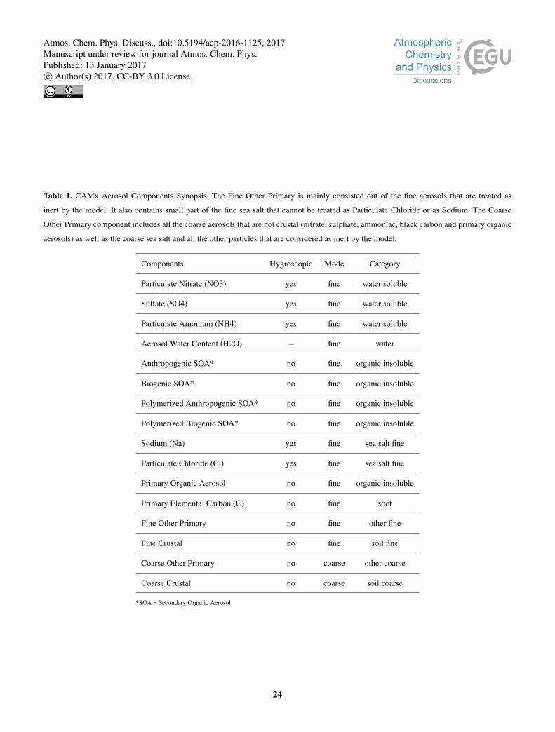
Table 1. CAMx Aerosol Components Synopsis. The Fine Other Primary is mainly consisted out of the fine aerosols that are treated as

inert by the model. It also contains small part of the fine sea salt that cannot be treated as Particulate Chloride or as Sodium. The Coarse

Other Primary component includes all the coarse aerosols that are not crustal (nitrate, sulphate, ammoniac, black carbon and primary organic

aerosols) as well as the coarse sea salt and all the other particles that are considered as inert by the model.

Components Hygroscopic Mode Category

Particulate Nitrate (NO3) yes fine water soluble

Sulfate (SO4) yes fine water soluble

Particulate Amonium (NH4) yes fine water soluble

Aerosol Water Content (H2O) – fine water

Anthropogenic SOA* no fine organic insoluble

Biogenic SOA* no fine organic insoluble

Polymerized Anthropogenic SOA* no fine organic insoluble

Polymerized Biogenic SOA* no fine organic insoluble

Sodium (Na) yes fine sea salt fine

Particulate Chloride (Cl) yes fine sea salt fine

Primary Organic Aerosol no fine organic insoluble

Primary Elemental Carbon (C) no fine soot

Fine Other Primary no fine other fine

Fine Crustal no fine soil fine

Coarse Other Primary no coarse other coarse

Coarse Crustal no coarse soil coarse

*SOA = Secondary Organic Aerosol

24


Table 2. Common Metrics Equations. The model data is defined as M and the lidar observational data as O. The a and c symbols correspond

to the height and the concentration respectively.

Metric Equation

Center of Mass

∫z·c·dz∫c·dz

Mean Bias1N

N∑i=1

(Mi−Oi)

Mean Fractional Bias (%)200N

N∑i=1

(Mi−Oi)(Mi+Oi)

RMSE [ 1N

N∑i=1

(Mi−Oi)2]

12

25


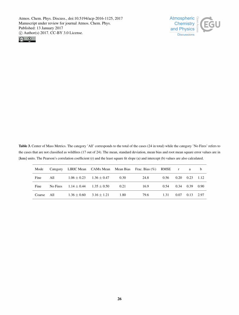
Table 3. Center of Mass Metrics. The category ’All’ corresponds to the total of the cases (24 in total) while the category ’No Fires’ refers to

the cases that are not classified as wildfires (17 out of 24). The mean, standard deviation, mean bias and root mean square error values are in

[km] units. The Pearson’s correlation coefficient (r) and the least square fit slope (a) and intercept (b) values are also calculated.

Mode Category LIRIC Mean CAMx Mean Mean Bias Frac. Bias (%) RMSE r a b

Fine All 1.06 ± 0.23 1.36 ± 0.47 0.30 24.8 0.56 0.20 0.23 1.12

Fine No Fires 1.14 ± 0.44 1.35 ± 0.50 0.21 16.9 0.54 0.34 0.39 0.90

Coarse All 1.36 ± 0.60 3.16 ± 1.21 1.80 79.6 1.31 0.07 0.13 2.97

26


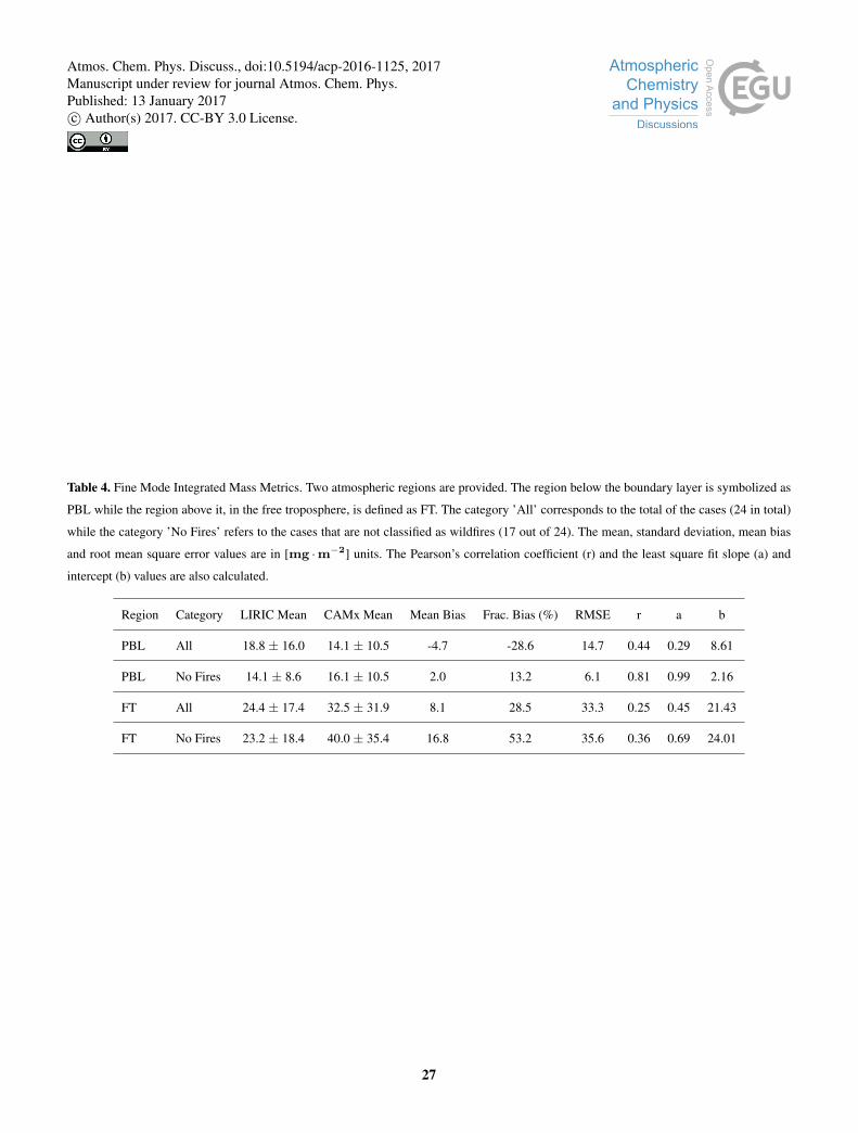
Table 4. Fine Mode Integrated Mass Metrics. Two atmospheric regions are provided. The region below the boundary layer is symbolized as

PBL while the region above it, in the free troposphere, is defined as FT. The category ’All’ corresponds to the total of the cases (24 in total)

while the category ’No Fires’ refers to the cases that are not classified as wildfires (17 out of 24). The mean, standard deviation, mean bias

and root mean square error values are in [mg ·m−2] units. The Pearson’s correlation coefficient (r) and the least square fit slope (a) and

intercept (b) values are also calculated.

Region Category LIRIC Mean CAMx Mean Mean Bias Frac. Bias (%) RMSE r a b

PBL All 18.8 ± 16.0 14.1 ± 10.5 -4.7 -28.6 14.7 0.44 0.29 8.61

PBL No Fires 14.1 ± 8.6 16.1 ± 10.5 2.0 13.2 6.1 0.81 0.99 2.16

FT All 24.4 ± 17.4 32.5 ± 31.9 8.1 28.5 33.3 0.25 0.45 21.43

FT No Fires 23.2 ± 18.4 40.0 ± 35.4 16.8 53.2 35.6 0.36 0.69 24.01

27


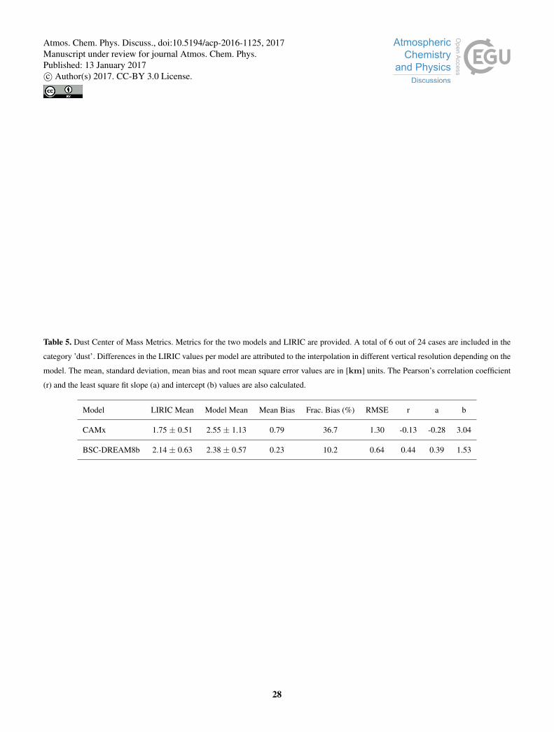
Table 5. Dust Center of Mass Metrics. Metrics for the two models and LIRIC are provided. A total of 6 out of 24 cases are included in the

category ’dust’. Differences in the LIRIC values per model are attributed to the interpolation in different vertical resolution depending on the

model. The mean, standard deviation, mean bias and root mean square error values are in [km] units. The Pearson’s correlation coefficient

(r) and the least square fit slope (a) and intercept (b) values are also calculated.

Model LIRIC Mean Model Mean Mean Bias Frac. Bias (%) RMSE r a b

CAMx 1.75 ± 0.51 2.55 ± 1.13 0.79 36.7 1.30 -0.13 -0.28 3.04

BSC-DREAM8b 2.14 ± 0.63 2.38 ± 0.57 0.23 10.2 0.64 0.44 0.39 1.53

28


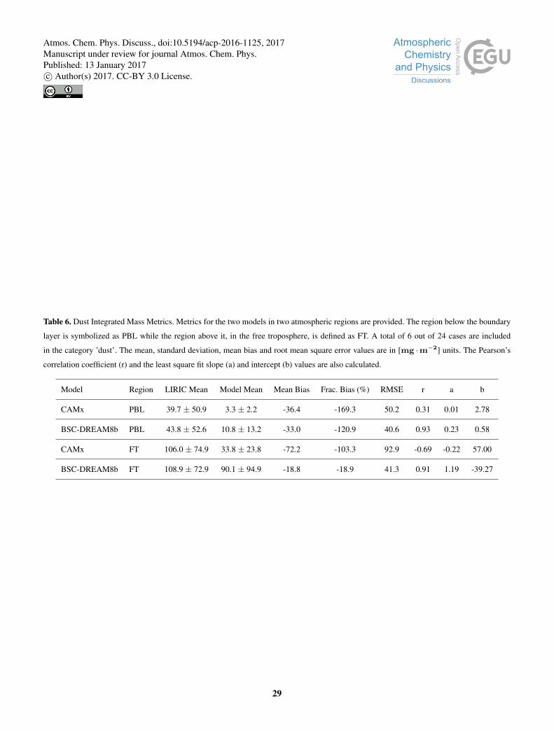
Table 6. Dust Integrated Mass Metrics. Metrics for the two models in two atmospheric regions are provided. The region below the boundary

layer is symbolized as PBL while the region above it, in the free troposphere, is defined as FT. A total of 6 out of 24 cases are included

in the category ’dust’. The mean, standard deviation, mean bias and root mean square error values are in [mg ·m−2] units. The Pearson’s

correlation coefficient (r) and the least square fit slope (a) and intercept (b) values are also calculated.

Model Region LIRIC Mean Model Mean Mean Bias Frac. Bias (%) RMSE r a b

CAMx PBL 39.7 ± 50.9 3.3 ± 2.2 -36.4 -169.3 50.2 0.31 0.01 2.78

BSC-DREAM8b PBL 43.8 ± 52.6 10.8 ± 13.2 -33.0 -120.9 40.6 0.93 0.23 0.58

CAMx FT 106.0 ± 74.9 33.8 ± 23.8 -72.2 -103.3 92.9 -0.69 -0.22 57.00

BSC-DREAM8b FT 108.9 ± 72.9 90.1 ± 94.9 -18.8 -18.9 41.3 0.91 1.19 -39.27

29


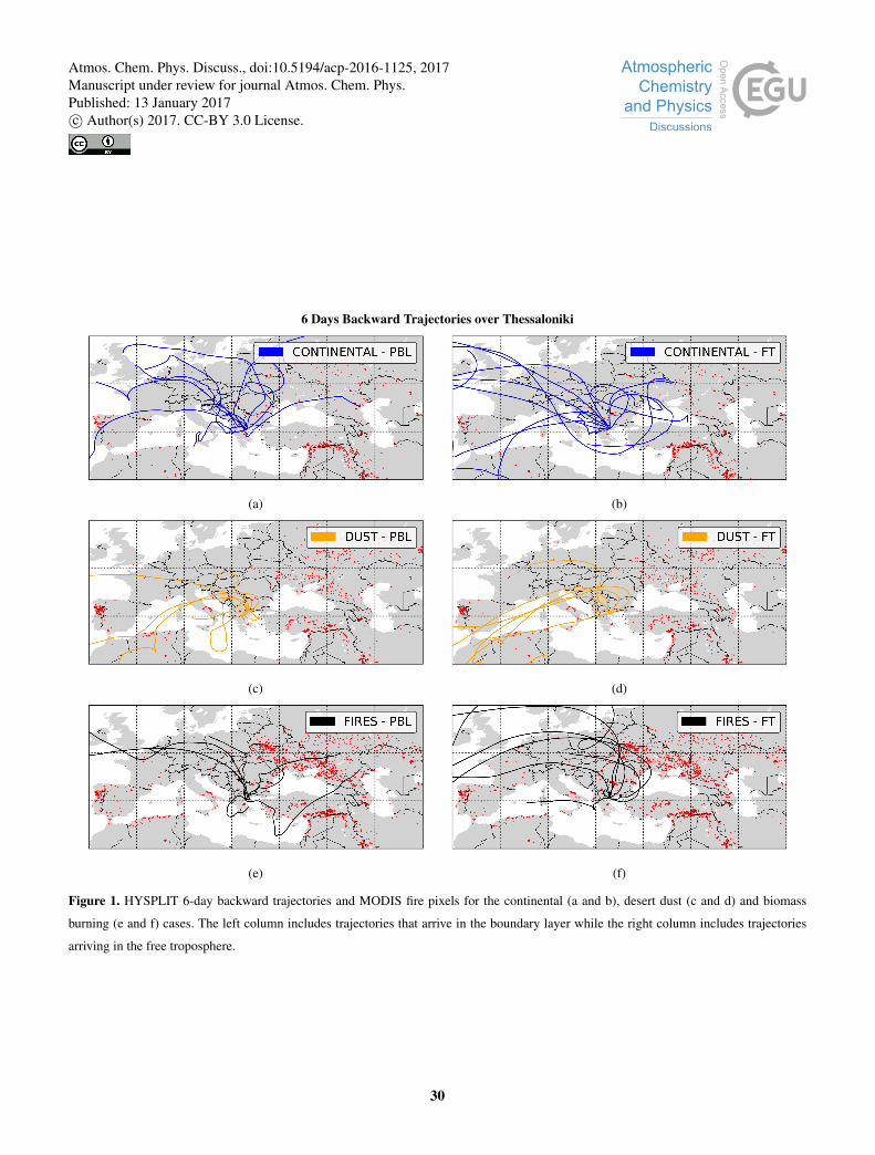
6 Days Backward Trajectories over Thessaloniki

(a) (b)

(c) (d)

(e) (f)

Figure 1. HYSPLIT 6-day backward trajectories and MODIS fire pixels for the continental (a and b), desert dust (c and d) and biomass

burning (e and f) cases. The left column includes trajectories that arrive in the boundary layer while the right column includes trajectories

arriving in the free troposphere.

30


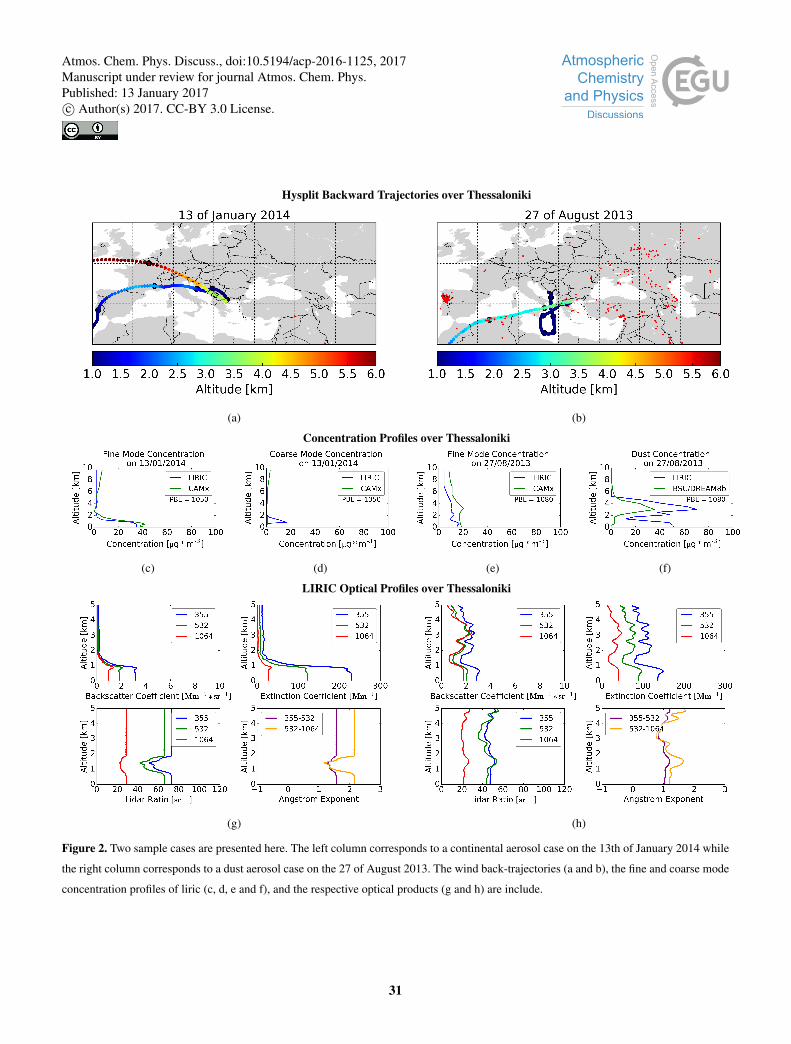
Hysplit Backward Trajectories over Thessaloniki

(a) (b)

Concentration Profiles over Thessaloniki

(c) (d) (e) (f)

LIRIC Optical Profiles over Thessaloniki

(g) (h)

Figure 2. Two sample cases are presented here. The left column corresponds to a continental aerosol case on the 13th of January 2014 while

the right column corresponds to a dust aerosol case on the 27 of August 2013. The wind back-trajectories (a and b), the fine and coarse mode

concentration profiles of liric (c, d, e and f), and the respective optical products (g and h) are include.

31


LIRIC and CAMx Concentration Profiles

(a) (b)

CAMx Aerosol Component Profiles

(c) (d)

Figure 3. a and b: Comparison of the mean fine mode (a) and coarse mode (b) aerosol concentration profiles between LIRIC and CAMx.

The shaded regions correspond to one σ of each average profile.

c and d: Presentation of the mean concentration profiles per aerosol component out of which the model’s fine mode (c) and coarse mode (d)

are consisted (see table 1).

32


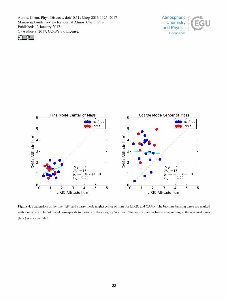
Figure 4. Scatterplots of the fine (left) and coarse mode (right) center of mass for LIRIC and CAMx. The biomass burning cases are marked

with a red color. The ’nf’ label corresponds to metrics of the category ’no fires’. The least square fit line corresponding to the screened cases

(blue) is also included.

33


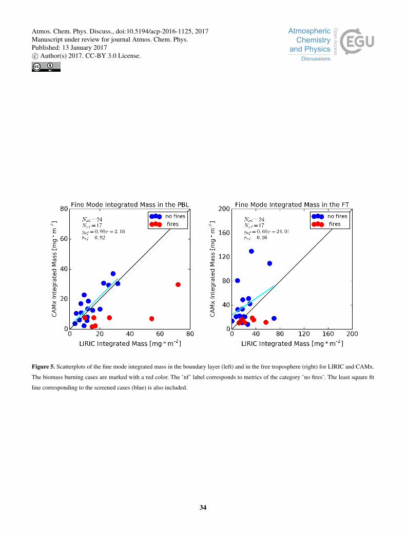
Figure 5. Scatterplots of the fine mode integrated mass in the boundary layer (left) and in the free troposphere (right) for LIRIC and CAMx.

The biomass burning cases are marked with a red color. The ’nf’ label corresponds to metrics of the category ’no fires’. The least square fit

line corresponding to the screened cases (blue) is also included.

34


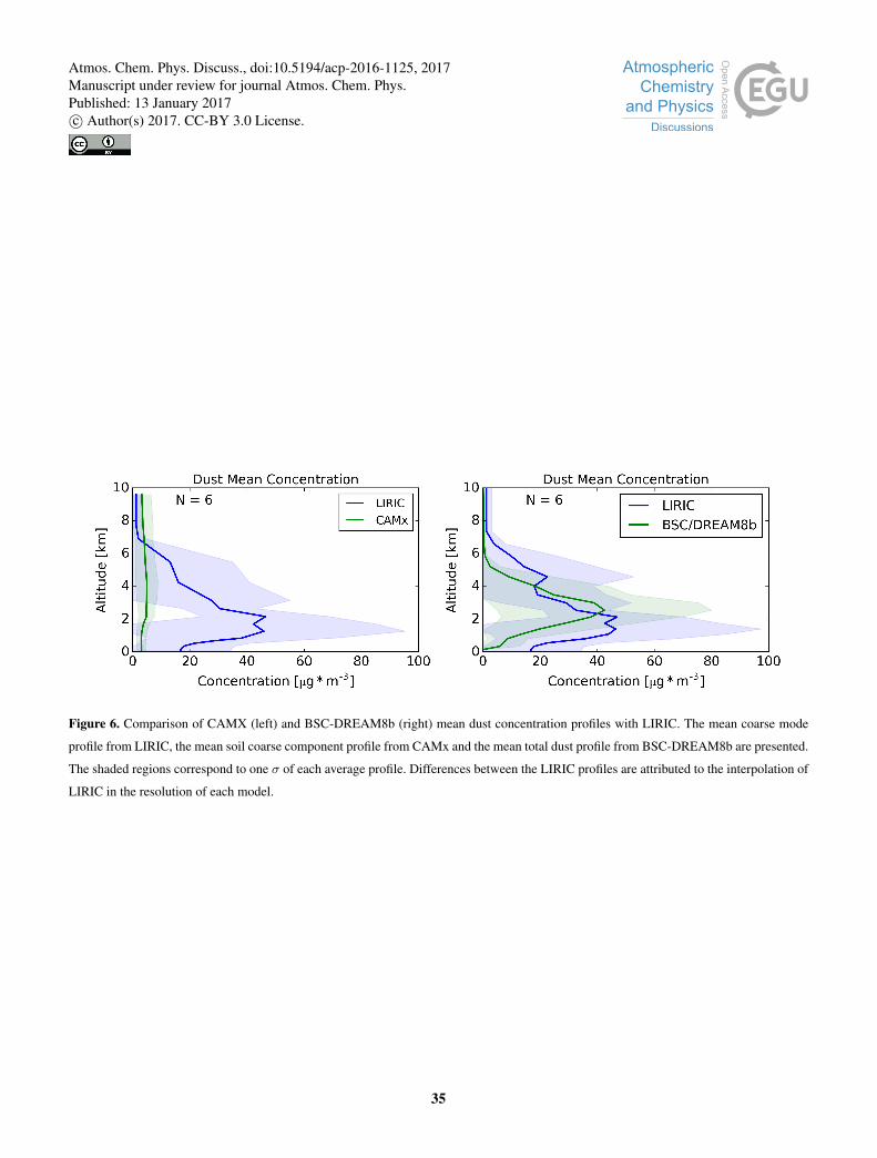
Figure 6. Comparison of CAMX (left) and BSC-DREAM8b (right) mean dust concentration profiles with LIRIC. The mean coarse mode

profile from LIRIC, the mean soil coarse component profile from CAMx and the mean total dust profile from BSC-DREAM8b are presented.

The shaded regions correspond to one σ of each average profile. Differences between the LIRIC profiles are attributed to the interpolation of

LIRIC in the resolution of each model.

35


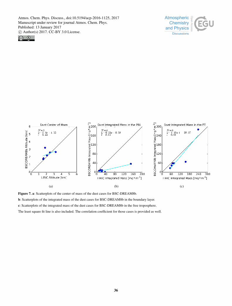
(a) (b) (c)

Figure 7. a: Scatterplots of the center of mass of the dust cases for BSC-DREAM8b.

b: Scatterplots of the integrated mass of the dust cases for BSC-DREAM8b in the boundary layer.

c: Scatterplots of the integrated mass of the dust cases for BSC-DREAM8b in the free troposphere.

The least square fit line is also included. The correlation coefficient for those cases is provided as well.

36


investigating the quality of modeled aerosol profiles based on

Documents