investigating topology control and cognitive radios to
TRANSCRIPT

Investigating Topology Control and Cognitive Radios to Exploit
Television Whitespace in Building Sparse Broadband Networks
Ivan R. Judson
September 28, 2011

Abstract
Described in this paper is my proposed Ph.D. thesis research which is to investigate the use of televisionwhitespace (TVWS) to build sparse broadband networks. In order to overcome topographical, environ-mental, and power issues the approach I propose is to use a topology control solution that uses TVWS toconnect smaller, localized networks. These smaller local networks are traditional wireless networks thathave been augmented with a set of cognitive radios that can route traffic between the local wireless networkand the topology control network. Additionally, I propose to investigate the dynamic, periodic election ofthese gateway nodes to ensure robust connectivity; one approach I propose to investigate for the dynamicelection of gateway nodes is using Game Theory. This paper includes a discussion of the backgroundrelevant to the proposed topic including wireless technology - including recently available whitespace fre-quencies, rural broadband issues and solutions, topographical and weather issues that arise. This paperalso includes a presentation of the progress made to this point and proposes a plan for future research.

Contents
1 Introduction 11.1 Motivation . . . . . . . . . . . . . . . . . . . . . . . . . . . . . . . . . . . . . . . . . . . . . 21.2 Contents . . . . . . . . . . . . . . . . . . . . . . . . . . . . . . . . . . . . . . . . . . . . . . . 2
2 Background 32.1 Wireless Networking Fundamentals . . . . . . . . . . . . . . . . . . . . . . . . . . . . . . . . 52.2 Frequency Selection . . . . . . . . . . . . . . . . . . . . . . . . . . . . . . . . . . . . . . . . 5
2.2.1 Whitespace Frequency Allocation . . . . . . . . . . . . . . . . . . . . . . . . . . . . . 62.3 Radios . . . . . . . . . . . . . . . . . . . . . . . . . . . . . . . . . . . . . . . . . . . . . . . . 6
2.3.1 Cognitive Radios . . . . . . . . . . . . . . . . . . . . . . . . . . . . . . . . . . . . . . 62.4 Antennas . . . . . . . . . . . . . . . . . . . . . . . . . . . . . . . . . . . . . . . . . . . . . . 72.5 Power . . . . . . . . . . . . . . . . . . . . . . . . . . . . . . . . . . . . . . . . . . . . . . . . 72.6 Challenges . . . . . . . . . . . . . . . . . . . . . . . . . . . . . . . . . . . . . . . . . . . . . . 7
2.6.1 Population Density . . . . . . . . . . . . . . . . . . . . . . . . . . . . . . . . . . . . . 82.6.2 Topography . . . . . . . . . . . . . . . . . . . . . . . . . . . . . . . . . . . . . . . . . 82.6.3 Environment . . . . . . . . . . . . . . . . . . . . . . . . . . . . . . . . . . . . . . . . 82.6.4 Power . . . . . . . . . . . . . . . . . . . . . . . . . . . . . . . . . . . . . . . . . . . . 92.6.5 Cost . . . . . . . . . . . . . . . . . . . . . . . . . . . . . . . . . . . . . . . . . . . . . 9
2.7 Literature Review . . . . . . . . . . . . . . . . . . . . . . . . . . . . . . . . . . . . . . . . . 92.7.1 Rural Wireless Networking . . . . . . . . . . . . . . . . . . . . . . . . . . . . . . . . 92.7.2 Whitespace Frequency Usage . . . . . . . . . . . . . . . . . . . . . . . . . . . . . . . 102.7.3 Smart Antennas . . . . . . . . . . . . . . . . . . . . . . . . . . . . . . . . . . . . . . 102.7.4 Topology Control . . . . . . . . . . . . . . . . . . . . . . . . . . . . . . . . . . . . . . 102.7.5 Cognitive Radios . . . . . . . . . . . . . . . . . . . . . . . . . . . . . . . . . . . . . . 112.7.6 Joint Routing and Channel Selection . . . . . . . . . . . . . . . . . . . . . . . . . . . 112.7.7 Game Theory in Wireless Networking . . . . . . . . . . . . . . . . . . . . . . . . . . 11
2.8 Computational Complexity . . . . . . . . . . . . . . . . . . . . . . . . . . . . . . . . . . . . 11
3 Current Work 133.1 In Situ Wireless Network: The Buffalo Jump Technology Cooperative . . . . . . . . . . . . 133.2 Topology Control in Multihop Wireless Networks with Multi-beam Smart Antennas . . . . 14
3.2.1 System Model . . . . . . . . . . . . . . . . . . . . . . . . . . . . . . . . . . . . . . . . 153.2.2 Problem Formulation . . . . . . . . . . . . . . . . . . . . . . . . . . . . . . . . . . . 163.2.3 Simulation Results . . . . . . . . . . . . . . . . . . . . . . . . . . . . . . . . . . . . . 163.2.4 Conclusions . . . . . . . . . . . . . . . . . . . . . . . . . . . . . . . . . . . . . . . . . 17
3.3 Beam Scheduling . . . . . . . . . . . . . . . . . . . . . . . . . . . . . . . . . . . . . . . . . . 173.3.1 System Model . . . . . . . . . . . . . . . . . . . . . . . . . . . . . . . . . . . . . . . . 183.3.2 Problem Formulation . . . . . . . . . . . . . . . . . . . . . . . . . . . . . . . . . . . 193.3.3 Proposed Algorithms . . . . . . . . . . . . . . . . . . . . . . . . . . . . . . . . . . . . 203.3.4 Simulation Results . . . . . . . . . . . . . . . . . . . . . . . . . . . . . . . . . . . . . 213.3.5 Conclusions . . . . . . . . . . . . . . . . . . . . . . . . . . . . . . . . . . . . . . . . . 23
3.4 Channel Selection and Joint Routing and Channel Selection in Cognitive Radio Networks . 23

3.4.1 Problem Formulation . . . . . . . . . . . . . . . . . . . . . . . . . . . . . . . . . . . 243.4.2 Proposed Algorithms . . . . . . . . . . . . . . . . . . . . . . . . . . . . . . . . . . . . 283.4.3 Simulation Results . . . . . . . . . . . . . . . . . . . . . . . . . . . . . . . . . . . . . 283.4.4 Conclusions . . . . . . . . . . . . . . . . . . . . . . . . . . . . . . . . . . . . . . . . . 30
4 Research Plan 314.1 Research Goals . . . . . . . . . . . . . . . . . . . . . . . . . . . . . . . . . . . . . . . . . . . 314.2 Extensions to Current Work . . . . . . . . . . . . . . . . . . . . . . . . . . . . . . . . . . . . 31
4.2.1 Topography . . . . . . . . . . . . . . . . . . . . . . . . . . . . . . . . . . . . . . . . . 314.2.2 Whitespace . . . . . . . . . . . . . . . . . . . . . . . . . . . . . . . . . . . . . . . . . 324.2.3 Beam Refinement . . . . . . . . . . . . . . . . . . . . . . . . . . . . . . . . . . . . . . 32
4.3 Future Work . . . . . . . . . . . . . . . . . . . . . . . . . . . . . . . . . . . . . . . . . . . . 324.3.1 A Sparse Broadband Network Architecture . . . . . . . . . . . . . . . . . . . . . . . 32
4.4 Timeline . . . . . . . . . . . . . . . . . . . . . . . . . . . . . . . . . . . . . . . . . . . . . . . 35
Bibliography 36
Chapter 1
Introduction
Broadband internet connectivity has become an assumed resource in most of the first world, in secondworld nations most of the population has broadband access through modern cellular networks. One of thelargest factors that affect the quality and coverage of robust broadband infrastructure is population density.This is drives the investment in expensive terrestrial broadband infrastructure. Further exacerbating thedeployment of this infrastructure, if remote users are not only in sparsely populated areas, but in areaswhere terrain and weather drive the need for more dense infrastructure the deployment and maintenancecosts increase. These regions of highly varying terrain with low population densities can be found all overthe world.
Residents of these areas typically do not have access to broadband internet; if they do, it’s a costlyservice that is unfortunately unaffordable for many with a fairly low performance. Examples includeWildBlue [1] and HughesNet [2] satellite internet which cost approximately $80 per month or $960 peryear and provide bandwidths of approximately 1-2Mbps down and 200-400kbps up, which is not classifiedas broadband according to the Federal Communications Commission [3]. Historically, when there hasbeen no commercial opportunity for technology deployment and maintenance, one of two solutions - or acombination of both - have been used to solve the problem: the rural cooperative model or the stimulationof commercial interest through federal funding.
Wireless networking provides a strong basic solution to the problem of providing broadband to citizenslocated where there is insufficient cost justification for wired infrastructure. However, the same cost problemexists for the commercial wireless broadband market because that infrastructure involves the same highcost infrastructure requiring a high population density to justify the cost. Wireless towers can cost inexcess of $1M, which necessitates that they are deployed in areas where there are enough subscribers tojustify the cost. Expensive infrastructure, either terrestrial (Fiber, Co-location spaces) and wireless requirea significant investment and therefore a minimum population density to make them commercially viable,therefore they are not present in areas with a population density below that threshold.
How then can a society move towards a digitally engaged citizenry when as much as 20% of thepopulace has no broadband access? There are two solutions: rely on the commercial market, who throughtax-based incentives and subsidies lower the threshold of population density and invest in the infrastructurerequired to reach the remaining citizens with broadband, or enable the citizens to cost-effectively providebroadband infrastructure for themselves. The latter solution has been used in rural areas for hundreds ofyears, it’s call the cooperative. Historically, cooperatives were goods based, agriculture, crafts, or otherproducts, but increasingly cooperatives have become organizations of scale, engaging in both the buyingand selling of goods, but also services for the members of the cooperative. Electrification of rural Americanwas accomplished through federal funding of electrical cooperatives, the same legislation that broughtelectricity to rural America has more recently been used to justify fiber based broadband infrastructuredeployments.
1

1.1 Motivation
However in order to overcome the technical issues involved in the deployment and maintenance of technicalinfrastructure work must be done to ensure the technology is simple to setup, easy to maintain and costeffective. The market is driving the cost-effectiveness by driving down costs of wireless components andproducts. There are now multiple vendors providing lost cost wireless devices with high-bandwidth, avariety of frequencies, and ruggedized hardware. Some of these vendors are also providing open platformsfor research and development. Tools from the vendors include more and more setup and maintenancesupport enabling non-technical end-users to setup, deploy and maintain a wireless infrastructure.
There is, however, still work to create robust planning tools and better architectures and algorithmsto provide the most robust infrastructure possible. My ultimate goal is to build a toolkit of hardware,software, and documentation that provides everything necessary for the smallest, least technologicallyendowed populations to implement their own broadband infrastructure and participate in the increasinglydigital world. In order to build this toolkit there are a set of fundamental technologies that must bedeveloped. In particular, there are solutions needed to numerous hardware, software and social challenges.Fundamental research needs to be engaged that will provide robust wireless solutions, open hardwareplatforms upon which research can happen, and locations where test networks can be deployed and studiedfor long periods of time. As more and more resources are discovered and re-discovered, such as unlicensedaccess to TV whitespace, research needs to incorporate these resources into their proposed solutions tothe problem of sparse broadband solutions. By breaking this problem down into a well structured set ofparameters, I hope to develop a highly robust set of algorithms and resources that can be used to solvethe larger problem of broadband for rural regions.
I propose to investigates three specific areas that can improve existing and future wireless infrastruc-ture in rural and/or sparsely populated regions with highly varying topography: extending existing beamscheduling, beam selection, and routing/channel selection simulations to three dimensions and include TVwhite space frequencies, using a game theoretic solution to the selection of backbone gateway nodes fromlocal wireless clouds and then simulating a sparse broadband network architecture in sparsely populated,highly varying terrain.
1.2 Contents
The sum of this proposal is organized into sections including background on wireless networking with anemphasis on sparse, highly varying terrain, a research plan, evaluation criteria and the expected contri-butions of this research. The background section includes an overview of relevant wireless networkingfundamentals, a deep, rich literature review, and a summary of my previous work. My research planaddresses three specific sub-problems and how I plan to solve those problems, the evaluation section de-scribes the papers, software, and simulations I propose to produce as evidence of successfully solving thethree sub-problems I have chosen. Contributions are summarized in the that section including the papers,software, documentation, and implementation of a solution that I propose.
2

Chapter 2
Background
Rural broadband connectivity continues to be a challenge even as technology continues to improve networking-related products and services. The driving factor is population density, which relates directly to the recoveryof infrastructure costs. In areas of low population density there are not enough customers to cover the nec-essary infrastructure that can enable cost-effective infrastructure investment. The challenges of developingrural broadband are similar to the challenges this nation faced when rural electrification was an issue. Asrecently as the 1930s, 90% of rural homes and farms were without electricity. After the federal governmentstepped in and enabled rural electric cooperatives in 1935, the installation of electrical systems spreadquickly; by 1953 more than 90% of rural homes and farms had electricity.
Delivering broadband networking to sparsely populated parts of America is a continuing challenge.Terrestrial broadband, using fiber or copper networking, requires the same investment in rural areas asin sub-urban and urban areas. However, in rural areas there are many fewer customers to share the costof the infrastructure which makes the cost per customer of the infrastructure unattractive to commercialproviders. This has left many rural residents with few options for internet access; often only two alternativesexistsatellite internet or cellular broadband.
The federal government and several non-governmental research and public policy organizations haveconducted in-depth examinations of the extent of broadband infrastructure in the US, and the results allpoint to the same conclusions: a significant gap remains between the availability of high-speed internetservices in rural areas relative to metropolitan and suburban areas [4–6]. These reports further identifymajor differences in the typical speeds of networks in rural areas relative to metro area networks, and thatrural users are paying higher prices for lower quality services. While some argue that the demographics ofrural areas do not generate the demand for broadband network investment, the evidence has repeatedlyshown that the availability of broadband infrastructure leads to economic growth, higher quality educationand healthcare services, and more citizen engagement in community, state and federal services.
There are essentially three tiers of internet access: 1) locations with broadband (cable-modem and/ordigital subscriber line) internet, 2) locations with satellite and/or cellular broadband, and 3) areas whereno service of any kind is available. Cable-modem and DSL customers are privileged to have significantlyhigher bandwidths than satellite and cellular customers, and they also benefit from significantly lowercosts. Satellite and cellular broadband are differentiable from cable-modem or digital subscriber lines(DSL) because they have bandwidth limits. The bandwidth limits throttle the network connection orcharge additional fees, after a certain amount of bandwidth is used.
Satellite and cellular broadband are not equivalent to options like cable-modem and digital subscriberlines (DSL) available in densely populated areas. While satellite and cellular solutions can provide relativelyhigh throughput, they do not provide low latency, and cost significantly more than cable-modem and DSL.Satellite and cellular solutions often have bandwidth usage policies that are enforced by limiting or disablingthe internet connection or charge significant fees for additional usage. While these bandwidth pricingmodels make sense in order for the providers to maintain competitiveness and still provide internet accessto rural areas, there are better and more cost-effective models that dont suffer from the same constraints.
Because rural broadband can be enabled using wireless technology, it is possible to build the necessaryinfrastructure with significantly reduced costs; there are no long-haul networking connections to put in
3

place. All wireless networking requires is wireless nodes deployed in proximity of other wireless nodes andelectricity to each wireless node [7, 8]. Wireless internet service providers (WISPS) are already providingaccess to many communities, but their reach is limited by what is economically viable for their business.Technology cooperatives can fill the gap. Technology cooperatives, like rural electrical cooperatives, canoperate without the same profit constraints as other providers and deploy a wireless network solution bysharing the cost among the members.
With the recent conversion of television from analog to digital transmission, an additional portion ofradio spectrum has been made available to unlicensed wireless use. The availability of more radio spectrumand the potential to use lower frequencies via the TV white spaces initiative than are currently used byWiFi networks (e.g., 2.4 GHz) offers enormous potential for rural area networks. Radio signal range D isgoverned by a frequency-dependent power law relationship. In areas where there is a clear, line of sightpath, where f is the frequency, and in areas where he antenna hight is low or where there are significantobstructions, the range is considerably less. Furthermore, lower frequency radio signals propagate aroundobstructions, whereas the higher frequency signals are blocked. Hence the use of TV white space spectrumat 500 MHz could lead to an extension in range by a factor of 25 or more relative to one that operates inthe current 2.4 GHz band used by most WiFi systems.
As an example, Montana’s Gallatin County has an average population density of twenty-five people persquare mile, estimated to reach approximately 45 people per square mile in 2030, according to the 2000U.S. Census Bureau, Montana Department of Commerce, and the Gallatin County Planning Department.If a single radio, antenna and power system can be constructed for $250 and cover that same squaremile, then for $10 per person per square mile startup costs, plus ongoing maintenance and service feesof approximately $5 per person per month, the entire county could provide a bare minimum of wirelessbroadband to everyone. Quadrupling the cost to $40 per person for startup expenses, plus $20 per monthfor operations would enable construction of a moderately robust system with significantly more capabilities,and the cost would still not approach the typical $250 startup, plus $75 per month costs of alternativesolutions [9]. A recent examination of the life cycle costs for deploying and operating wireless fixed internetaccess in Gallatin county communities, in areas not covered by current wire line systems, yielded similarresults [7].
There are a few challenges that inhibit the average citizen from building a wireless cloud. The choiceof hardware, antennas, locations that include electricity, and the ongoing maintenance and operation ofthe wireless network are not effort-free using today’s technology. In fact it takes expert network operatorsand technicians to design, install, deploy and support existing WISP installations. Fortunately, many ofthese questions can be simplified through robust software and testing infrastructure, enabling end users todeploy wireless with minimal effort and a high success rate.
Efforts like MIT’s RoofNet [10] – which was commercialized as Meraki, Inc. [11], FreiFunk [12], Open-WRT [13], and Open-Mesh are providing hardware and software that solves many of the associated issuesfor high-density urban and suburban populations. Much of the existing work is focused on communitieswhere population density is high and electricity is relatively easy to access. Ubiquiti Networks, Inc. hasbeen incorporating these lessons into the software they use to drive the comprehensive hardware solutionsthey have been developing and presents a product line that is commercially available, robust, flexible, andcan be extended and enhanced by our proposed work.
Some projects have been reported that address the distances typical of rural area networks. WILDNet,for example, was built by a group at the University of California, Berkeley, using conventional WiFitechnology operating at 2.4GHz [14]. Their demonstration network yielded high throughput over distancesof up to 50-100km, obtained by making minor adjustments to the radio system protocols. Other work, usingWiMAX (IEEE 802.16d) shows comparable results [15], and this technology is now being put in place forfixed wireless access in several networks in developing countries where conventional wireline infrastructureis poor or nonexistent. These projects provide excellent solutions for point-to-point, long distance links,which could link remote areas, but they don’t provide a solution for a local area network that doesn’t haveline of sight.
Projects in high population density areas make sense because the impact, the ratio of affected usersto cost, is high; however, defining the impact with this ratio immediately defines areas of low populationdensity as areas of low impact. Its not until this digital division produces significant enough disparitybetween high impact and low impact opportunities to be identified as inequitable that these definitions
4

change. Our aim is to find an efficient, cost effective solution for areas of low population density to avoidthe widening of the digital divide and enable rural communities to participate in the opportunities affordedby broadband internet access.
2.1 Wireless Networking Fundamentals
The fundamental difference is wireless and wired networking is that wireless networking uses radios toconvert bits to radio frequencies instead of electrical signals conducted by wires. From an application pointof view any differences in networking protocols are hidden in the operating system and driver software,presenting a uniform network interface. The radios used in wireless networking come in a variety of differentconfigurations, supporting a growing number of different wireless networking standards. The configurationvariations include radio frequency, antenna types, radio capabilities, and radio power output.
A typical wireless network consists of one or more gateways, providing access for users of the wirelessnetwork to resources outside of the wireless network, these act similarly to consumer internet routers likea cable, DSL or satellite modem. The most common consumer network connects the modem directly toa computer, but more and more consumers are inserting wireless routers into the modem providing theability for more than one computer to share the internet connection. Similarly, in a wireless network theinternet gateways are connected to a set of relay nodes that provide the core routing functionality of thenetwork. These relay nodes track each other and reconfigure the network as needed to provide the highestperformance for the users possible. The users in a wireless network are traditionally named SubscriberNodes, since they are subscribing to wireless services where there may be multiple choices for services.
There are multiple wireless network architectures but the most common are: a tree, where the root isthe internet gateway, the internal nodes are the relay nodes and the leaves are the subscribers; the mesh,where there can be one or more internet gateways, a set of relay nodes, and a set of subscribers; and aladder, where there are two internet gateways, relay nodes configured in two parallel lines, and subscribersfollow the lines. These architectures correspond to the most common functions of wireless networking:enterprise networking, cellular/sensor/environmental networking, and transportation networking.
Consumer wireless networking has been traditionally done in the 2.4GHz and 5GHz frequency space, butmore recently devices using the 900MHz range have become available, offering more choice to consumers.Power output (and thus consumption) is not a typical factor for most wireless network implementations,but when installed in remote locations where power is not available it becomes a significant influence ondesign. Similarly, most radios have an integrated antenna, providing basic coverage for a typical usagescenario – but more and more radios are providing external antenna connectors to enable augmenting theradio with higher powered antennas to improve range and performance. Most consumer wireless productsdo not have advanced capabilities – like the ability to sense signals and adapt their configuration to adjustfor performance – however some products have been emerging with an open software platform allowingaftermarket modification to enable these types of advanced functions.
2.2 Frequency Selection
The frequencies available for unlicensed use are a fairly small part of the overall radio spectrum, typicallyin the 700-900MHz, 2.4GHz, and 5.8GHz regions. These frequencies provide very different transmissioncharacteristics with the 5.8GHz providing higher bandwidth, but at a significantly shorter distance thanthe 700-900MHz range. However the lower frequencies typically provide lower bandwidth, although recentdevelopments with multiple frequency, multiple antenna, and MIMO-type radios ensure that solutions atalmost any frequency provide robust, high bandwidth for the end users.
One aspect of the different frequencies are the propagation characteristics and the performance in thepresence of interference (from weather, foliage, or other intermittent obstruction). The higher the frequen-cies, e.g. 5.8GHz, there is less penetration of solid objects and there is more sensitivity to obstructions.The lower frequency signals are able to penetrate better, go farther, and are less vulnerable to signalobstruction.
5

U.S.
DEPARTMENT OF COMMERC
ENA
TION
AL TELEC
OM
M
UNICATIONS & INFORMATION
AD
MIN
ISTR
ATI
ON
MO
BILE
(AE
RONA
UTIC
AL T
ELEM
ETER
ING
)
S)
5.68
5.73
5.90
5.95
6.2
6.52
5
6.68
56.
765
7.0
7.1
7.3
7.35
8.1
8.19
5
8.81
5
8.96
59.
040
9.4
9.5
9.9
9.99
510
.003
10.0
0510
.110
.15
11.1
7511
.275
11.4
11.6
11.6
5
12.0
5
12.1
0
12.2
3
13.2
13.2
613
.36
13.4
113
.57
13.6
13.8
13.8
714
.014
.25
14.3
5
14.9
9015
.005
15.0
1015
.10
15.6
15.8
16.3
6
17.4
1
17.4
817
.55
17.9
17.9
718
.03
18.0
6818
.168
18.7
818
.919
.02
19.6
819
.80
19.9
9019
.995
20.0
0520
.010
21.0
21.4
521
.85
21.9
2422
.0
22.8
5523
.023
.223
.35
24.8
924
.99
25.0
05
25.0
125
.07
25.2
125
.33
25.5
525
.67
26.1
26.1
7526
.48
26.9
526
.96
27.2
327
.41
27.5
428
.0
29.7
29.8
29.8
929
.91
30.0
UNITEDSTATES
THE RADIO SPECTRUM
NON-GOVERNMENT EXCLUSIVE
GOVERNMENT/ NON-GOVERNMENT SHAREDGOVERNMENT EXCLUSIVE
RADIO SERVICES COLOR LEGEND
ACTIVITY CODE
NOT ALLOCATED RADIONAVIGATION FIXED
MARITIME MOBILEFIXED
MARITIME MOBILE
FIXED
MARITIME MOBILE
Radiolocation RADIONAVIGATION
FIXED
MARITIMEMOBILE
Radiolocation
FIXED
MARITIMEMOBILE
FIXED
MARITIMEMOBILE
AERONAUTICALRADIONAVIGATION
AERO
NAUT
ICAL
RADI
ONAV
IGAT
ION
Aero
naut
ical
Mob
ile
Mar
itime
Radi
onav
igat
ion
(Rad
io Be
acon
s)M
ARIT
IME
RADI
ONAV
IGAT
ION
(RAD
IO B
EACO
NS)
Aero
naut
ical
Radi
onav
igat
ion
(Rad
io Be
acon
s)
3 9 14 19.9
5
20.0
5
30 30 59 61 70 90 110
130
160
190
200
275
285
300
3 kHz 300 kHz
300 kHz 3 MHz
3 MHz 30 MHz
30 MHz 300 MHz
3 GHz
300 GHz
300 MHz
3 GHz
30 GHz
AeronauticalRadionavigation(Radio Beacons)
MARITIMERADIONAVIGATION(RADIO BEACONS)
Aero
naut
ical
Mob
ile
Mar
itime
Radio
navig
ation
(Rad
io Be
acon
s)
AERO
NAUT
ICAL
RADI
ONAV
IGAT
ION
(RAD
IO B
EACO
NS)
AERONAUTICALRADIONAVIGATION(RADIO BEACONS)
AeronauticalMobile
Aero
naut
ical M
obile
RADI
ONAV
IGAT
ION
AER
ONA
UTIC
ALRA
DIO
NAVI
GAT
ION
MAR
ITIM
EM
OBI
LE AeronauticalRadionavigation
MO
BILE
(DIS
TRES
S AN
D CA
LLIN
G)
MAR
ITIM
E M
OBI
LE
MAR
ITIM
EM
OBI
LE(S
HIPS
ONL
Y)
MO
BILE
AERO
NAUT
ICAL
RADI
ONA
VIG
ATIO
N(R
ADIO
BEA
CONS
)
AERO
NAUT
ICAL
RADI
ONAV
IGAT
ION
(RAD
IO B
EACO
NS)
BROADCASTING(AM RADIO)
MAR
ITIM
E M
OBI
LE (T
ELEP
HONY
)
MAR
ITIM
E M
OBI
LE (T
ELEP
HONY
) M
OBI
LE (D
ISTR
ESS
AND
CALL
ING
)
MARITIMEMOBILE
LAND MOBILE
MOBILE
FIXED STAN
DARD
FRE
Q. A
ND T
IME
SIG
NAL
(250
0kHz
)
STAN
DARD
FRE
Q. A
ND T
IME
SIG
NAL
Spac
e Re
sear
ch MARITIMEMOBILE
LAND MOBILE
MOBILE
FIXED
AERO
NAUT
ICAL
MOB
ILE
(R)
STAN
DARD
FRE
Q.
AERO
NAUT
ICAL
MO
BILE
(R)
AERO
NAUT
ICAL
MOB
ILE
(OR)
AERO
NAUT
ICAL
MOB
ILE
(R)
FIXED
MOBILE**
Radio-location
FIXE
DM
OBI
LE*
AMATEUR
FIXE
D
FIXE
D
FIXE
D
FIXED
FIXE
DMARITIMEMOBILE
MO
BILE
*
MO
BILE
*
MO
BILE
STAN
DARD
FRE
Q. A
ND T
IME
SIG
NAL
(500
0 KH
Z)
AERO
NAUT
ICAL
MO
BILE
(R)
AERO
NAUT
ICAL
MO
BILE
(OR)
STAN
DARD
FRE
Q.
Spac
e Re
sear
ch
MOBILE**
AERO
NAUT
ICAL
MO
BILE
(R)
AERO
NAUT
ICAL
MO
BILE
(OR) FIX
ED
MO
BILE
*
BRO
ADCA
STIN
G
MAR
ITIM
E M
OBI
LE
AERO
NAUT
ICAL
MO
BILE
(R)
AERO
NAUT
ICAL
MO
BILE
(OR) FIXE
DM
obile
AMAT
EUR
SATE
LLIT
EAM
ATEU
R
AMAT
EUR
FIXED
Mobile
MAR
ITIM
E M
OBILE
MARITIMEMOBILE
AERO
NAUT
ICAL
MO
BILE
(R)
AERO
NAUT
ICAL
MO
BILE
(OR)
FIX
ED
BRO
ADCA
STIN
G
FIXE
DST
ANDA
RD F
REQ
. AND
TIM
E SI
GNA
L (1
0,00
0 kH
z)ST
ANDA
RD F
REQ
.Sp
ace
Rese
arch
AERO
NAUT
ICAL
MO
BILE
(R)
AMAT
EUR
FIXED
Mobile* AERO
NAUT
ICAL
MO
BILE
(R)
AERO
NAUT
ICAL
MO
BILE
(OR)
FIXE
D
FIXE
DBRO
ADCA
STIN
G
MAR
ITIM
EM
OBI
LE
AERO
NAUT
ICAL
MOB
ILE (R
)
AERO
NAUT
ICAL
MOB
ILE (O
R)
RADI
O AS
TRON
OMY
Mob
ile*
AMAT
EUR
BRO
ADCA
STIN
G
AMAT
EUR
AMAT
EUR
SATE
LLIT
E
Mob
ile*
FIXE
D
BRO
ADCA
STIN
G
STAN
DARD
FRE
Q. A
ND T
IME
SIG
NAL
(15,
000
kHz)
STAN
DARD
FRE
Q.
Spac
e Re
sear
ch
FIXED
AERO
NAUT
ICAL
MO
BILE
(OR)
MAR
ITIM
EM
OBI
LE
AERO
NAUT
ICAL
MO
BILE
(OR)
AERO
NAUT
ICAL
MO
BILE
(R)
FIXE
D
FIXE
D
BRO
ADCA
STIN
G
STAN
DARD
FRE
Q.
Spac
e Re
sear
ch
FIXE
D
MAR
ITIM
E M
OBI
LE
Mob
ileFI
XED
AMAT
EUR
AMAT
EUR
SATE
LLIT
E
BRO
ADCA
STIN
GFI
XED
AERO
NAUT
ICAL
MO
BILE
(R)
MAR
ITIM
E M
OBI
LE
FIXE
DFI
XED
FIXE
D
Mob
ile*
MO
BILE
**
FIXE
D
STAN
DARD
FRE
Q. A
ND T
IME
SIG
NAL
(25,
000
kHz)
STAN
DARD
FRE
Q.
Spac
e Re
sear
ch
LAN
D M
OBI
LEM
ARIT
IME
MO
BILE
LAN
D M
OBI
LE M
OBI
LE**
RAD
IO A
STRO
NOM
YBR
OAD
CAST
ING
MAR
ITIM
E M
OBI
LE L
AND
MO
BILE
FIXE
D M
OBI
LE**
FIXE
D
MO
BILE
**
MO
BILE
FIXE
D
FIXE
D
FIXE
DFI
XED
FIXE
D
LAND
MOB
ILE
MO
BILE
**
AMAT
EUR
AMAT
EUR
SATE
LLIT
E
MO
BILE
LAN
D M
OBI
LE
MO
BILE
MO
BILE
FIXE
D
FIXE
D
MO
BILE
MO
BILE
FIXE
D
FIXE
D
LAN
DM
OBI
LE
LAN
DM
OBI
LE
LAN
DM
OBI
LE
LAND
MO
BILE
Radi
o As
trono
my
RADI
O AS
TRON
OMY
LAND
MO
BILE
FIXE
DFI
XED
MO
BILEMOB
ILE
MOBILE
LAND
MO
BILE
FIXED
LAN
DM
OBI
LE
FIXE
D
FIXE
D
MO
BILE
MOB
ILE
LANDMOBILE AMATEUR
BROADCASTING(TV CHANNELS 2-4)
FIXE
DM
OBI
LE
FIXE
DM
OBI
LE
FIXE
DM
OBI
LEFI
XED
MO
BILE
AERO
NAUT
ICAL
RAD
IONA
VIG
ATIO
N
BROADCASTING(TV CHANNELS 5-6)
BROADCASTING(FM RADIO)
AERONAUTICALRADIONAVIGATION
AER
ON
AUTI
CAL
MO
BILE
(R)
AERO
NAUT
ICAL
MO
BILE
AERO
NAUT
ICAL
MO
BILE
AER
ON
AUTI
CAL
MO
BILE
(R)
AER
ON
AUTI
CAL
MO
BILE
(R)
AERO
NAUT
ICAL
MO
BILE
(R)
MO
BILE
FIX
ED
AMAT
EUR
BROADCASTING(TV CHANNELS 7-13)
MOBILE
FIXED
MOBILE
FIXED
MOBILE SATELLITE
FIXED
MOBILESATELLITE
MOBILE
FIXED
MOBILESATELLITE
MOBILE
FIXE
DM
OBI
LE
AERO
NAUT
ICAL
RAD
IONA
VIG
ATIO
N
STD.
FRE
Q. &
TIM
E SI
GNAL
SAT
. (40
0.1
MHz
)ME
T. SA
T.(S
-E)
SPAC
E RE
S.(S
-E)
Earth
Exp
l.Sa
tellit
e (E
-S)
MO
BILE
SAT
ELLI
TE (E
-S)
FIXE
DM
OBI
LERA
DIO
ASTR
ONOM
Y
RADI
OLO
CATI
ON
Amat
eur
LAND
MO
BILE
MeteorologicalSatellite (S-E)
LAND
MO
BILE
BROA
DCAS
TING
(TV C
HANN
ELS 1
4 - 20
)
BROADCASTING(TV CHANNELS 21-36)
TV BROADCASTINGRAD
IO A
STR
ON
OM
Y
RADI
OLO
CATI
ON
FIXE
D
Amat
eur
AERONAUTICALRADIONAVIGATION
MO
BILE
**FI
XED
AERO
NAUT
ICAL
RADIO
NAVIG
ATION
Radi
oloc
atio
n
Radi
oloc
atio
nM
ARIT
IME
RADI
ONA
VIG
ATIO
N
MAR
ITIM
ERA
DIO
NAVI
GAT
ION
Radi
oloc
atio
n
Radiolocation
Radiolocation
RADIO-LOCATION RADIO-
LOCATION
Amateur
AERO
NAUT
ICAL
RADI
ONAV
IGAT
ION
(Gro
und)
RADI
O-LO
CATI
ONRa
dio-
locat
ion
AERO
. RAD
IO-
NAV.
(Grou
nd)
FIXED
SAT.
(S-E
)RA
DIO-
LOCA
TION
Radio
-loc
ation
FIXED
FIXEDSATELLITE
(S-E)
FIXE
D
AERO
NAUT
ICAL
RAD
IONA
VIG
ATIO
N MO
BILE
FIXE
DM
OBI
LE
RADI
O A
STRO
NOM
YSp
ace
Rese
arch
(Pas
sive)
AERO
NAUT
ICAL
RAD
IONA
VIG
ATIO
N
RADI
O-
LOCA
TIO
NRa
dio-
loca
tion
RADI
ONA
VIG
ATIO
N
Radi
oloc
atio
n
RADI
OLO
CATI
ON
Radi
oloc
atio
n
Radi
oloc
atio
n
Radi
oloc
atio
n
RADI
OLO
CATI
ON
RADI
O-
LOCA
TIO
N
MAR
ITIM
ERA
DIO
NAVI
GAT
ION
MAR
ITIM
ERA
DION
AVIG
ATIO
NM
ETEO
ROLO
GIC
ALAI
DS
Amat
eur
Amat
eur
FIXED
FIXE
DSA
TELL
ITE
(E-S
)M
OBIL
E
FIXE
DSA
TELL
ITE
(E-S
)
FIXE
DSA
TELL
ITE
(E-S
)M
OB
ILE
FIXE
D FIXE
D
FIXE
D
FIXE
D
MOB
ILE
FIXE
DSP
ACE
RESE
ARCH
(E-S
)FI
XED
Fixe
dM
OBIL
ESA
TELL
ITE
(S-E
)FIX
ED S
ATEL
LITE
(S-E
)
FIXED
SAT
ELLIT
E (S
-E)
FIXED
SATE
LLITE
(S-E
)
FIXE
DSA
TELL
ITE
(S-E
)
FIXE
DSA
TELL
ITE
(E-S
)FI
XED
SATE
LLIT
E (E
-S) FIX
EDSA
TELL
ITE(E
-S) FIX
EDSA
TELL
ITE(E
-S)
FIXE
D
FIXE
D
FIXE
D
FIXE
D
FIXE
D
FIXE
D
FIXE
D
MET.
SATE
LLITE
(S-E
)M
obile
Satel
lite (S
-E)
Mob
ileSa
tellite
(S-E
)
Mobil
eSa
tellite
(E-S
)(no
airb
orne)
Mobil
e Sa
tellite
(E-S
)(no
airbo
rne)
Mobil
e Sa
tellite
(S-E
)
Mob
ileSa
tellite
(E-S
)
MOB
ILE
SATE
LLIT
E (E
-S)
EART
H EX
PL.
SATE
LLITE
(S-E
)
EART
H EX
PL.
SAT.
(S-E
)
EART
H EX
PL.
SATE
LLITE
(S-E
)
MET.
SATE
LLITE
(E-S
)
FIXE
D
FIXE
D
SPAC
E RE
SEAR
CH (S
-E)
(dee
p sp
ace
only)
SPAC
E RE
SEAR
CH (S
-E)
AERO
NAUT
ICAL
RADI
ONA
VIG
ATIO
N
RADI
OLO
CATI
ON
Radi
oloc
atio
n
Radi
oloc
atio
n
Radio
locat
ion
Radio
locat
ion
MAR
ITIM
ERA
DIO
NAVI
GAT
ION M
eteo
rolog
ical
Aids
RADI
ONAV
IGAT
ION
RADI
OLO
CATI
ON
Radi
oloc
atio
n
RADI
O-
LOCA
TIO
N
Radio
locati
on
Radio
locat
ionAm
ateu
r
Amat
eur
Amat
eur
Sate
llite
RADI
OLO
CATI
ON
FIXE
D
FIXE
D
FIXED
FIX
EDFIXED
SATELLITE(S-E)
FIXEDSATELLITE
(S-E)
Mobile **
SPAC
E RE
SEAR
CH(P
assiv
e)EA
RTH
EXPL
.SA
T. (P
assiv
e)RA
DIO
ASTR
ONOM
Y
SPAC
ERE
SEAR
CH (P
assiv
e)EA
RTH
EXPL
.SA
TELL
ITE
(Pas
sive)
RADI
OAS
TRO
NOM
Y
BRO
ADCA
STIN
GSA
TELL
ITE
AERO
NAUT
ICAL
RAD
IONA
V.Sp
ace
Rese
arch
(E-S
)
SpaceResearch
Land
Mob
ileSa
tellite
(E-S
)
Radio
-loc
ation
RADI
O-LO
CATI
ON
RADI
ONA
VIGA
TION FI
XE
DSA
TELL
ITE
(E-S
)La
nd M
obile
Sate
llite
(E-
S)
Land
Mob
ileSa
tellite
(E-S
)Fi
xed
Mob
ileFI
XED
SAT
. (E-
S)
Fixe
dM
obile
FIXE
D
Mob
ileFI
XED
MOB
ILE
Spac
e Re
sear
chSp
ace
Rese
arch
Spac
e Re
sear
ch
SPAC
E RE
SEAR
CH(P
assiv
e)RA
DIO
ASTR
ONOM
YEA
RTH
EXPL
. SAT
.(P
assiv
e)
Radio
locati
on
RADI
OLO
CATI
ON
Radi
oloc
atio
n
FX S
AT (
E-S)
FIXE
D SA
TELL
ITE
(E-
S)FI
XE
D
FIXE
D
FIX
ED
MO
BIL
E
EART
H EX
PL.
SAT.
(Pas
sive)
MO
BIL
E
Earth
Exp
l.Sa
tellite
(Acti
ve)
Stan
dard
Freq
uenc
y an
dTim
e Si
gnal
Satel
lite (E
-S)
Earth
Explo
ratio
nSa
tellit
e(S
-S)
MOB
ILE
FIXE
D
MO
BIL
E
FIX
ED
Earth
Explo
ratio
nSa
tellite
(S-S
)
FIX
ED
MO
BIL
EFI
XE
DSA
T (E
-S)
FIXE
D SA
TELL
ITE
(E-S
)M
OBIL
E SA
TELL
ITE
(E-S
)
FIXE
DSA
TELL
ITE
(E-S
)
MOB
ILE
SATE
LLIT
E(E
-S)
Stan
dard
Freq
uenc
y an
dTim
e Si
gnal
Satel
lite (S
-E)
Stan
d. Fr
eque
ncy
and
Time
Sign
alSa
tellite
(S-E
)FI
XED
MOB
ILE
RADI
OAS
TRO
NOM
YSP
ACE
RESE
ARCH
(Pas
sive)
EART
HEX
PLOR
ATIO
NSA
T. (P
assiv
e)
RADI
ONA
VIG
ATIO
N
RADI
ONA
VIG
ATIO
NIN
TER-
SATE
LLIT
E
RADI
ONA
VIG
ATIO
N
RADI
OLO
CATI
ON
Radi
oloc
atio
n
SPAC
E R
E..(
Pass
ive)
EART
H EX
PL.
SAT.
(Pas
sive)
FIX
ED
MO
BIL
E
FIX
ED
MO
BIL
E
FIX
ED
MOB
ILE
Mob
ileFi
xedFIXE
DSA
TELL
ITE
(S-E
)
BR
OA
D-
CA
STI
NG
BC
ST
SA
T.
FIXE
DM
OBIL
E
FX
SAT(
E-S)
MO
BIL
EFI
XE
D
EART
HEX
PLO
RATI
ON
SATE
LLIT
EFI
XED
SATE
LLITE
(E-S
)MO
BILE
SATE
LLITE
(E-S
)
MO
BIL
EFI
XE
D
SP
AC
ER
ES
EA
RC
H(P
assi
ve)
EART
HEX
PLOR
ATIO
NSA
TELL
ITE
(Pas
sive)
EART
HEX
PLOR
ATIO
NSA
T. (P
assiv
e)
SPAC
ERE
SEAR
CH(P
assiv
e)
INTE
R-SA
TELL
ITE
RADI
O-LO
CATIO
N
SPAC
ERE
SEAR
CHFI
XE
D
MOBILE
F IXED
MOBILESATELLITE
(E-S)
MOB
ILESA
TELL
ITE
RADI
ONA
VIGA
TION
RADI
O-NA
VIGA
TION
SATE
LLIT
E
EART
HEX
PLOR
ATIO
NSA
TELL
ITE F IXED
SATELLITE(E-S)
MOB
ILE
FIXE
DFI
XED
SATE
LLIT
E (E
-S)
AMAT
EUR
AMAT
EUR
SATE
LLIT
E
AMAT
EUR
AMAT
EUR
SATE
LLIT
E
Amat
eur
Sate
llite
Amat
eur
RA
DIO
-LO
CAT
ION
MOB
ILE
FIXE
DM
OBIL
ESA
TELL
ITE
(S-E
)
FIXE
DSA
TELL
ITE
(S-E
)
MOB
ILE
FIXE
DBR
OAD
-CA
STIN
GSA
TELL
ITE
BRO
AD-
CAST
ING
SPACERESEARCH
(Passive)
RADIOASTRONOMY
EARTHEXPLORATION
SATELLITE(Passive)
MOBILE
FIX
ED
MOB
ILE
FIXE
DRA
DIO
-LO
CATI
ONFI
XED
SATE
LLIT
E(E
-S)
MOBILESATELLITE
RADIO-NAVIGATIONSATELLITE
RADIO-NAVIGATION
Radio-location
EART
H E
XPL.
SATE
LLIT
E (P
assiv
e)SP
ACE
RESE
ARCH
(Pas
sive)
FIX
ED
FIX
ED
SA
TELL
ITE
(S-E
)
SPACERESEARCH
(Passive)
RADIOASTRONOMY
EARTHEXPLORATION
SATELLITE(Passive)
FIXED
MOBILE
MO
BIL
EIN
TER-
SATE
LLIT
E
RADIO-LOCATION
INTER-SATELLITE
Radio-location
MOBILE
MOBILESATELLITE
RADIO-NAVIGATION
RADIO-NAVIGATIONSATELLITE
AMAT
EUR
AMAT
EUR
SATE
LLIT
E
Amat
eur
Amat
eur S
atel
liteRA
DIO
-LO
CATI
ON
MOB
ILE
FIXE
DFI
XED
SATE
LLIT
E (S
-E)
MOB
ILE
FIXE
DFI
XED
SATE
LLIT
E(S
-E)
EART
HEX
PLOR
ATIO
NSA
TELL
ITE
(Pas
sive)
SPAC
E RE
S.(P
assiv
e)
SPAC
E RE
S.(P
assiv
e)
RADI
OAS
TRO
NOM
Y
FIXEDSATELLITE
(S-E)
FIXED
MOB
ILE
FIXE
D
MOB
ILE
FIXE
D
MOB
ILE
FIXE
D
MOB
ILE
FIXE
D
MOB
ILE
FIXE
D
SPAC
E RE
SEAR
CH(P
assiv
e)RA
DIO
ASTR
ONO
MY
EART
HEX
PLOR
ATIO
NSA
TELL
ITE
(Pas
sive)
EART
HEX
PLOR
ATIO
NSA
T. (P
assiv
e)
SPAC
ERE
SEAR
CH(P
assiv
e)IN
TER-
SATE
LLIT
EINTE
R-SA
TELL
ITE
INTE
R-SA
TELL
ITE
INTE
R-SA
TELL
ITE
MOBILE
MOBILE
MOB
ILEMOBILE
SATELLITE
RADIO-NAVIGATION
RADIO-NAVIGATIONSATELLITE
FIXEDSATELLITE
(E-S)
FIXED
FIXE
DEA
RTH
EXPL
ORAT
ION
SAT.
(Pas
sive)
SPAC
E RE
S.(P
assiv
e)
SPACERESEARCH
(Passive)
RADIOASTRONOMY
EARTHEXPLORATION
SATELLITE(Passive)
MOB
ILE
FIXE
D
MOB
ILE
FIXE
D
MOB
ILE
FIXE
D
FIXE
DSA
TELL
ITE
(S-E
)
FIXE
DSA
TELL
ITE(
S-E) FI
XED
SATE
LLIT
E (S
-E)
EART
H EX
PL.
SAT.
(Pas
sive)
SPAC
E RE
S.(P
assiv
e)
Radi
o-lo
catio
n
Radi
o-lo
catio
n
RADI
O-
LOCA
TION
AMAT
EUR
AMAT
EUR
SATE
LLIT
E
Amat
eur
Amat
eur S
atel
lite
EART
H EX
PLO
RATI
ON
SATE
LLIT
E (P
assiv
e)SP
ACE
RES.
(Pas
sive)
MOBILE
MOBILESATELLITE
RADIO-NAVIGATION
RADIO-NAVIGATIONSATELLITE
MOBILE
MOBILE
FIXED
RADIO-ASTRONOMY
FIXEDSATELLITE
(E-S)
FIXED
3.0
3.02
5
3.15
5
3.23
0
3.4
3.5
4.0
4.06
3
4.43
8
4.65
4.7
4.75
4.85
4.99
55.
003
5.00
55.
060
5.45
MARITIMEMOBILE
AMAT
EUR
AMAT
EUR
SATE
LLIT
EFI
XED
Mob
ileM
ARIT
IME
MOB
ILE
STAN
DARD
FRE
QUEN
CY &
TIM
E SI
GNAL
(20,
000
KHZ)
Spac
e Re
sear
ch
AERO
NAUT
ICAL
MO
BILE
(OR)
AMAT
EUR
SATE
LLIT
EAM
ATEU
R
MET.
SAT.
(S-E
)MO
B. S
AT. (S
-E)
SPAC
E RE
S. (S
-E)
SPAC
E OP
N. (S
-E)
MET.
SAT.
(S-E
)Mo
b. Sa
t. (S-
E)SP
ACE
RES.
(S-E
)SP
ACE
OPN.
(S-E
)ME
T. SA
T. (S
-E)
MOB.
SAT
. (S-E
)SP
ACE
RES.
(S-E
)SP
ACE
OPN.
(S-E
)ME
T. SA
T. (S
-E)
Mob.
Sat. (
S-E)
SPAC
E RE
S. (S
-E)
SPAC
E OP
N. (S
-E)
MOBILE
FIXED
FIXE
DLa
nd M
obile
FIXE
DM
OBIL
E
LAN
D M
OBIL
E
LAN
D MO
BILE
MAR
ITIM
E MO
BILE
MAR
ITIM
E MO
BILE
MAR
ITIM
E M
OBIL
E
MAR
ITIM
E MO
BILE
LAN
D M
OBIL
E
FIXE
DM
OBI
LEMO
BILE
SATE
LLITE
(E-S
)
Radi
oloc
atio
n
Radio
locat
ionLA
ND M
OBIL
EAM
ATEU
R
MOB
ILE S
ATEL
LITE
(E-S
) R
ADIO
NAVI
GATI
ON S
ATEL
LITE
MET
. AID
S(R
adios
onde
)
MET
EORO
LOGI
CAL
AIDS
(RAD
IOSO
NDE)
SPAC
E R
ESEA
RCH
(S-S
)FI
XED
MO
BILE
LAND
MO
BILE
FIXE
DLA
ND M
OBI
LE
FIXE
DFI
XED
RADI
O A
STRO
NOM
Y
RADI
O A
STRO
NOM
YM
ETEO
ROLO
GIC
ALAI
DS (R
ADIO
SOND
E)
MET
EORO
LOG
ICAL
AIDS
(Rad
ioso
nde)
MET
EORO
LOG
ICAL
SATE
LLIT
E (s
-E)
Fixed
FIXED
MET. SAT.(s-E)
FIX
ED
FIXE
D
AERO
NAUT
ICAL
MOB
ILE S
ATEL
LITE
(R) (
spac
e to
Earth
)
AERO
NAUT
ICAL
RAD
IONA
VIGAT
ION
RADI
ONAV
. SAT
ELLIT
E (S
pace
to E
arth)
AERO
NAUT
ICAL
MOB
ILE S
ATEL
LITE
(R)
(spac
e to E
arth)
Mobile
Sate
llite (
S- E
)
RADI
O DE
T. SA
T. (E
-S)
MO
BILE
SAT(
E-S)
AERO
. RAD
IONA
VIGAT
ION
AERO
. RAD
IONA
V.AE
RO. R
ADIO
NAV.
RADI
O DE
T. SA
T. (E
-S)
RADI
O DE
T. SA
T. (E
-S)
MOBIL
E SA
T. (E
-S)
MOBIL
E SAT
. (E-S
)Mo
bile S
at. (S
-E)
RADI
O AS
TRON
OMY
RADI
O A
STRO
NOM
Y M
OBIL
E SA
T. (
E-S)
FIXE
DM
OBI
LE
FIXE
D
FIXE
D(L
OS)
MOBI
LE(LO
S)SP
ACE
RESE
ARCH
(s-E)
(s-s)
SPAC
EOP
ERAT
ION
(s-E)
(s-s)
EART
HEX
PLOR
ATIO
NSA
T. (s-
E)(s-
s)
Amat
eur
MO
BILE
Fixe
dRA
DIOL
OCAT
ION
AMAT
EUR
RADI
O A
STRO
N.SP
ACE
RES
EAR
CH
EART
H E
XPL
SAT
FIXE
D SA
T. (S
-E)
FIXED
MOBILE
FIXEDSATELLITE (S-E)
FIXE
DM
OBIL
EFI
XED
SATE
LLIT
E (E
-S)
FIXE
DSA
TELL
ITE
(E-S
)M
OBIL
EFI
XED
SPAC
ERE
SEAR
CH (S
-E)
(Dee
p Sp
ace) AE
RONA
UTIC
AL R
ADIO
NAVI
GATI
ON
EART
HEX
PL. S
AT.
(Pas
sive)
300
325
335
405
415
435
495
505
510
525
535
1605
1615
1705
1800
1900
2000
2065
2107
2170
2173
.521
90.5
2194
2495
2501
2502
2505
2850
3000
RADIO-LOCATION
BRO
ADCA
STIN
G
FIXED
MOBILE
AMAT
EUR
RADI
OLOC
ATIO
N
MO
BILE
FIXE
DM
ARIT
IME
MO
BILE
MAR
ITIM
E M
OBI
LE (T
ELEP
HONY
)
MAR
ITIM
EM
OBIL
ELA
NDM
OBIL
EM
OBIL
EFI
XED
30.0
30.5
6
32.0
33.0
34.0
35.0
36.0
37.0
37.5
38.0
38.2
5
39.0
40.0
42.0
43.6
9
46.6
47.0
49.6
50.0
54.0
72.0
73.0
74.6
74.8
75.2
75.4
76.0
88.0
108.
0
117.
975
121.
9375
123.
0875
123.
5875
128.
8125
132.
0125
136.
0
137.
013
7.02
513
7.17
513
7.82
513
8.0
144.
014
6.0
148.
014
9.9
150.
05
150.
815
2.85
5
154.
0
156.
2475
157.
0375
157.
1875
157.
4516
1.57
516
1.62
516
1.77
516
2.01
25
173.
217
3.4
174.
0
216.
0
220.
022
2.0
225.
0
235.
0
300
ISM – 6.78 ± .015 MHz ISM – 13.560 ± .007 MHz ISM – 27.12 ± .163 MHz
ISM – 40.68 ± .02 MHz
ISM – 24.125 ± 0.125 GHz 30 GHz
ISM – 245.0 ± 1GHzISM – 122.5 ± .500 GHzISM – 61.25 ± .250 GHz
300.
0
322.
0
328.
6
335.
4
399.
9
400.
0540
0.15
401.
0
402.
0
403.
040
6.0
406.
1
410.
0
420.
0
450.
045
4.0
455.
045
6.0
460.
046
2.53
7546
2.73
7546
7.53
7546
7.73
7547
0.0
512.
0
608.
061
4.0
698
746
764
776
794
806
821
824
849
851
866
869
894
896
9019
01
902
928
929
930
931
932
935
940
941
944
960
1215
1240
1300
1350
1390
1392
1395
2000
2020
2025
2110
2155
2160
2180
2200
2290
2300
2305
2310
2320
2345
2360
2385
2390
2400
2417
2450
2483
.525
0026
5526
9027
00
2900
3000
1400
1427
1429
.5
1430
1432
1435
1525
1530
1535
1544
1545
1549
.5
1558
.515
5916
1016
10.6
1613
.816
26.5
1660
1660
.516
68.4
1670
1675
1700
1710
1755
1850
MARI
TIME
MOBIL
E SA
TELL
ITE(sp
ace t
o Eart
h)MO
BILE
SATE
LLITE
(S-E
)
RADI
OLO
CATI
ON
RADI
ONA
VIG
ATIO
NSA
TELL
ITE
(S-E
)
RADI
OLO
CATI
ON
Amat
eur
Radi
oloc
atio
nAE
RONA
UTIC
ALRA
DIO
NAVI
GAT
ION
SPA
CE
RESE
ARCH
( P
assiv
e)EA
RTH
EXP
L SA
T (Pa
ssive
)RA
DIO
A
STRO
NOMY
MO
BILE
MOB
ILE
**FI
XED-
SAT
(E
-S)
FIXE
D
FIXE
D FIXE
D**
LAND
MOB
ILE (T
LM)
MOBI
LE SA
T.(S
pace
to E
arth)
MARI
TIME
MOBI
LE S
AT.
(Spa
ce to
Eart
h)Mo
bile
(Aero
. TLM
)
MO
BILE
SAT
ELLI
TE (S
-E)
MOBIL
E SA
TELL
ITE(S
pace
to E
arth)
AERO
NAUT
ICAL
MOB
ILE S
ATEL
LITE
(R)
(spac
e to E
arth)
3.0
3.1
3.3
3.5
3.6
3.65
3.7
4.2
4.4
4.5
4.8
4.94
4.99
5.0
5.15
5.25
5.35
5.46
5.47
5.6
5.65
5.83
5.85
5.92
5
6.42
5
6.52
5
6.70
6.87
5
7.02
57.
075
7.12
5
7.19
7.23
57.
25
7.30
7.45
7.55
7.75
7.90
8.02
5
8.17
5
8.21
5
8.4
8.45
8.5
9.0
9.2
9.3
9.5
10.0
10.4
5
10.5
10.5
510
.6
10.6
8
10.7
11.7
12.2
12.7
12.7
5
13.2
513
.4
13.7
514
.0
14.2
14.4
14.4
714
.514
.714
5
15.1
365
15.3
5
15.4
15.4
3
15.6
315
.716
.6
17.1
17.2
17.3
17.7
17.8
18.3
18.6
18.8
19.3
19.7
20.1
20.2
21.2
21.4
22.0
22.2
122
.5
22.5
5
23.5
5
23.6
24.0
24.0
5
24.2
524
.45
24.6
5
24.7
5
25.0
5
25.2
525
.527
.0
27.5
29.5
29.9
30.0
ISM – 2450.0 ± 50 MHz
30.0
31.0
31.3
31.8
32.0
32.3
33.0
33.4
36.0
37.0
37.6
38.0
38.6
39.5
40.0
40.5
41.0
42.5
43.5
45.5
46.9
47.0
47.2
48.2
50.2
50.4
51.4
52.6
54.2
555
.78
56.9
57.0
58.2
59.0
59.3
64.0
65.0
66.0
71.0
74.0
75.5
76.0
77.0
77.5
78.0
81.0
84.0
86.0
92.0
95.0
100.
0
102.
0
105.
0
116.
0
119.
98
120.
02
126.
0
134.
0
142.
014
4.0
149.
0
150.
0
151.
0
164.
0
168.
0
170.
0
174.
5
176.
5
182.
0
185.
0
190.
0
200.
0
202.
0
217.
0
231.
0
235.
0
238.
0
241.
0
248.
0
250.
0
252.
0
265.
0
275.
0
300.
0
ISM – 5.8 ± .075 GHz
ISM – 915.0 ± 13 MHz
INTE
R-SA
TELL
ITE
RADI
OLOC
ATIO
NSA
TELL
ITE (E
-S)
AERO
NAUT
ICAL
RADI
ONAV
.
PLEASE NOTE: THE SPACING ALLOTTED THE SERVICES IN THE SPEC-TRUM SEGMENTS SHOWN IS NOT PROPORTIONAL TO THE ACTUAL AMOUNTOF SPECTRUM OCCUPIED.
AERONAUTICALMOBILE
AERONAUTICALMOBILE SATELLITE
AERONAUTICALRADIONAVIGATION
AMATEUR
AMATEUR SATELLITE
BROADCASTING
BROADCASTINGSATELLITE
EARTH EXPLORATIONSATELLITE
FIXED
FIXED SATELLITE
INTER-SATELLITE
LAND MOBILE
LAND MOBILESATELLITE
MARITIME MOBILE
MARITIME MOBILESATELLITE
MARITIMERADIONAVIGATION
METEOROLOGICALAIDS
METEOROLOGICALSATELLITE
MOBILE
MOBILE SATELLITE
RADIO ASTRONOMY
RADIODETERMINATIONSATELLITE
RADIOLOCATION
RADIOLOCATION SATELLITE
RADIONAVIGATION
RADIONAVIGATIONSATELLITE
SPACE OPERATION
SPACE RESEARCH
STANDARD FREQUENCYAND TIME SIGNAL
STANDARD FREQUENCYAND TIME SIGNAL SATELLITE
RADI
O A
STRO
NOM
Y
FIXED
MARITIME MOBILE
FIXED
MARITIMEMOBILE Aeronautical
Mobile
STAN
DARD
FRE
Q. A
ND T
IME
SIG
NAL
(60
kHz)
FIXE
DM
obile
*
STAN
D. F
REQ.
& T
IME
SIG.
MET.
AIDS
(Rad
ioson
de)
Spac
e Op
n. (S
-E)
MOBIL
E.SA
T. (S
-E)
Fixe
d
Stan
dard
Freq
. and
Time S
ignal
Satel
lite (E
-S)
FIXE
D
STAN
DARD
FRE
Q. A
ND T
IME
SIG
NAL
(20
kHz)
Amate
ur
MO
BIL
E
FIXE
D S
AT. (
E-S)
Spac
eRe
sear
ch
ALLOCATION USAGE DESIGNATION
SERVICE EXAMPLE DESCRIPTION
Primary FIXED Capital Letters
Secondary Mobi le 1st Capital with lower case letters
U.S. DEPARTMENT OF COMMERCENational Telecommunications and Information AdministrationOffice of Spectrum Management
October 2003
MO
BILE
BRO
ADCA
STIN
G
TRAVELERS INFORMATION STATIONS (G) AT 1610 kHz
59-64 GHz IS DESIGNATED FORUNLICENSED DEVICES
Fixed
AE
RO
NA
UTI
CA
LR
AD
ION
AV
IGA
TIO
N
SPAC
E RE
SEAR
CH (P
assiv
e)
* EXCEPT AERO MOBILE (R)
** EXCEPT AERO MOBILE WAVELENGTH
BANDDESIGNATIONS
ACTIVITIES
FREQUENCY
3 x 10⁷m 3 x 10⁶m 3 x 10⁵m 30,000 m 3,000 m 300 m 30 m 3 m 30 cm 3 cm 0.3 cm 0.03 cm 3 x 10⁵Å 3 x 10⁴Å 3 x 10³Å 3 x 10²Å 3 x 10Å 3Å 3 x 10⁻¹Å 3 x 10⁻²Å 3 x 10⁻³Å 3 x 10⁻⁴Å 3 x 10⁻⁵Å 3 x 10⁻⁶Å 3 x 10⁻⁷Å
0 10 Hz 100 Hz 1 kHz 10 kHz 100 kHz 1 MHz 10 MHz 100 MHz 1 GHz 10 GHz 100 GHz 1 THz 1013Hz 1014Hz 1015Hz 1016Hz 1017Hz 1018Hz 1019Hz 1020Hz 1021Hz 1022Hz 1023Hz 1024Hz 1025Hz
THE RADIO SPECTRUMMAGNIFIED ABOVE3 kHz 300 GHz
VERY LOW FREQUENCY (VLF)Audible Range AM Broadcast FM Broadcast Radar Sub-Millimeter Visible Ultraviolet Gamma-ray Cosmic-ray
Infra-sonics Sonics Ultra-sonics Microwaves Infrared
P L S XC RadarBands
LF MF HF VHF UHF SHF EHF INFRARED VISIBLE ULTRAVIOLET X-RAY GAMMA-RAY COSMIC-RAY
X-ray
ALLOCATIONSFREQUENCY
BR
OA
DC
AS
TIN
GFI
XE
DM
OB
ILE
*
BR
OA
DC
AS
TIN
GF
IXE
DB
RO
AD
CA
ST
ING
F
IXE
D
M
obile
FIX
ED
BR
OA
DC
AS
TIN
G
BROA
DCAS
TING
FIXE
D
FIXE
D
BRO
ADC
ASTI
NG
FIXE
DBR
OADC
ASTIN
GFI
XED
BROA
DCAS
TING
FIXE
D
BROA
DCAS
TING
FIXE
DBR
OADC
ASTIN
GFI
XED
BROA
DCAS
TING
FIXE
D
FIXE
D
FIXE
D
FIXE
DFI
XED
FIXE
D
LAN
DM
OBI
LE
FIX
ED
AERO
NAUT
ICAL
MO
BILE
(R)
AMAT
EUR
SATE
LLIT
EAM
ATEU
R MOB
ILE
SATE
LLIT
E (E
-S)
FIX
ED
Fixe
dM
obil
eR
adio
-lo
catio
nFI
XE
DM
OB
ILE
LAND
MO
BILE
MAR
ITIM
E M
OBIL
E
FIXE
D L
AND
MOB
ILE
FIXE
D
LAND
MO
BILE
RA
DIO
NA
V-S
AT
EL
LIT
E
FIXE
DM
OBI
LE
FIXE
D L
AND
MOB
ILE
MET.
AIDS
(Rad
io-so
nde)
SPAC
E OPN
. (S
-E)
Earth
Exp
l Sat
(E-S
)Me
t-Sate
llite
(E-S
)ME
T-SAT
. (E
-S)
EART
H EX
PLSA
T. (E
-S)
Earth
Exp
l Sat
(E-S
)Me
t-Sate
llite
(E-S
)EA
RTH
EXPL
SAT.
(E-S
)ME
T-SAT
. (E
-S)
LAND
MO
BILE
LAND
MO
BILE
FIXE
DLA
ND M
OBI
LEFI
XED
FIXE
D
FIXE
D L
AND
MOB
ILE
LAND
MO
BILE
FIXE
D L
AND
MOB
ILE
LAND
MO
BILE
LAN
D M
OBIL
E
LAND
MO
BILE
MO
BILE
FIXE
D
MO
BILE
FIXE
D
BRO
ADCA
STM
OBI
LEFI
XED
MO
BILE
FIXE
D
FIXE
DLA
ND M
OBI
LE LAND
MO
BILE
FIXE
DLA
ND M
OBI
LE AERO
NAUT
ICAL
MOB
ILE
AERO
NAUT
ICAL
MOB
ILE FIXE
DLA
ND M
OBI
LELA
ND M
OBI
LELA
ND M
OBI
LEFI
XED
LAND
MO
BILE
FIXE
DM
OB
ILE
FIXE
D
FIXE
DFI
XED
MO
BILE
FIXE
D
FIXE
DFI
XED
BRO
ADCA
ST
LAND
MO
BILE
LAND
MO
BILE
FIXE
DLA
ND M
OBI
LE
MET
EORO
LOGI
CAL
AIDS
FXSp
ace r
es.
Radi
o As
tE-
Expl
Sat
FIXE
DM
OBI
LE**
MOB
ILE
SATE
LLIT
E (S
-E)
RADI
ODET
ERMI
NATI
ON S
AT. (
S-E)
Radio
locati
onM
OBI
LEFI
XED
Amat
eur
Radio
locati
on
AM
ATE
UR
FIXE
DM
OBI
LE
B-SA
TFX
MO
BFi
xed
Mob
ileRa
diol
ocat
ion
RADI
OLO
CATI
ON
MOB
ILE
**
Fixed
(TLM
)LA
ND M
OBI
LEFI
XED
(TLM
)LA
ND M
OBI
LE (
TLM
)FI
XED-
SAT
(S
-E)
FIXE
D (T
LM)
MOB
ILE
MOBI
LE SA
T.(S
pace
to E
arth)
Mob
ile *
*
MO
BILE
**FI
XED
MO
BILE
MO
BILE
SAT
ELLI
TE (E
-S)
SPAC
E OP
.(E
-S)(s
-s)
EART
H EX
PL.
SAT.
(E-S)(
s-s)
SPAC
E RE
S.(E
-S)(s
-s)
FX.
MO
B.
MO
BILE
FIXE
D
Mob
ile
R- LO
C.
BCST
-SAT
ELLI
TEFi
xed
Radi
o-lo
catio
n
B-SA
TR-
LOC.
FXM
OB
Fixe
dM
obile
Radi
oloc
atio
nFI
XED
MO
BILE
**Am
ateu
rRA
DIOL
OCAT
ION
SPAC
E RE
S..(S
-E)
MO
BILE
FIXE
DM
OBI
LE S
ATEL
LITE
(S-E
)
MAR
ITIM
E M
OBI
LE
Mob
ile FIXE
D
FIXE
D
BRO
ADCA
STM
OBI
LEFI
XED
MO
BILE
SAT
ELLI
TE (E
-S)
FIXE
D
FIX
EDM
AR
ITIM
E M
OB
ILE
F
IXE
D
FIXE
DM
OBI
LE**
FIXE
DM
OBI
LE**
FIXE
D S
AT (S
-E)
AERO
. R
ADIO
NAV.
FIXE
DSA
TELL
ITE
(E-S
)
Amat
eur-
sat (
s-e)
Amat
eur
MO
BIL
EFI
XED
SAT
(E-S
)
FIX
ED
FIXE
D SA
TELL
ITE
(S-E
)(E-S
)
FIXE
DFI
XED
SAT
(E-S
)M
OB
ILE
Radio
-loc
ation
RADI
O-LO
CATI
ONF
IXE
D S
AT
.(E
-S)
Mob
ile**
Fixe
dM
obile
FX S
AT.(E
-S)
L M
Sat(E
-S)
AER
O
RAD
ION
AVFI
XED
SAT
(E-
S)
AERO
NAUT
ICAL
RAD
IONA
VIGA
TION
RADI
OLO
CATI
ON
Spac
e Re
s.(ac
t.)
RADI
OLO
CATI
ON
Radi
oloc
atio
n
Radio
loc.
RADI
OLOC
.Ea
rth E
xpl S
atSp
ace
Res.
Radio
locati
onBC
ST
SAT.
FIX
ED
FIXE
D SA
TELL
ITE
(S-
E)FI
XED
SAT
ELLI
TE (
S-E)
EART
H EX
PL. S
AT.
FX S
AT (
S-E)
SPAC
E RE
S.
FIXE
D S
ATEL
LITE
(S-
E)
FIXE
D S
ATEL
LITE
(S-
E)
FIXE
D S
ATEL
LITE
(S-
E)MO
BILE
SAT
. (S-
E)
FX S
AT (
S-E)
MO
BILE
SAT
ELLI
TE (
S-E)
FX S
AT (
S-E)
STD
FRE
Q. &
TIM
EMO
BILE
SAT
(S-E
)
EART
H EX
PL. S
AT.
MO
BIL
EFI
XE
DSP
ACE
RES. FI
XE
DM
OB
ILE
MO
BIL
E**
FIX
ED
EART
H EX
PL. S
AT.
FIX
ED
MOB
ILE*
*R
AD
.AS
TSP
ACE
RES.
FIX
ED
MO
BIL
E
INTE
R-SA
TELL
ITE
FIX
ED
RADI
O AS
TRON
OMY
SPAC
E R
ES.
(Pas
sive
)
AMAT
EUR
AMAT
EUR
SATE
LLIT
E
Radio
-loc
ation
Amate
urRA
DIO-
LOCA
TION
Earth
Ex
pl.
Sate
llite
(Act
ive)
FIX
ED
INTE
R-SA
TELL
ITE
RADI
ONAV
IGAT
ION
RADI
OLOC
ATIO
N
SAT
ELLIT
E (E-
S)IN
TER-
SATE
LLIT
E
FIX
ED
SA
TELL
ITE
(E-S
)RA
DION
AVIG
ATIO
N
FIX
ED
SA
TELL
ITE
(E-S
)FI
XE
D
MOB
ILE
SATE
LLIT
E (E
-S)
FIXE
D S
ATEL
LITE
(E-
S)
MO
BIL
EFI
XE
DEa
rth
Expl
orat
ion
Sate
llite
(S-S
)
std fre
q &
time
e-e
-sat
(s-s
)M
OB
ILE
FIX
ED
e-e
-sat
MO
BIL
E
SPAC
ERE
SEAR
CH (d
eep
spac
e)
RADI
ONA
VIG
ATIO
NIN
TER
- SA
TSP
ACE
RES
.
FIX
ED
MO
BIL
ESP
ACE
RES
EAR
CH
(spa
ce-to
-Ear
th)
SP
AC
ER
ES
.
FIX
ED
SAT.
(S-
E)M
OB
ILE
FIX
ED
FIXE
D-S
ATEL
LITE
MOB
ILE
FIX
ED
FIX
ED
SA
TELL
ITE
MO
BIL
ES
AT.
FIX
ED
SA
TM
OB
ILE
SA
T.EA
RTH
EXPL
SAT
(E-S
)
Earth
Expl
.Sa
t (s
- e)
SPAC
E R
ES. (
E-S)
FX-S
AT(S
-E)
FIXE
DM
OBIL
EB
RO
AD
-C
AS
TIN
GB
CS
TS
AT.
RADI
OAS
TRON
OMY
FIX
ED
MO
BIL
E**
FIXE
DSA
TELL
ITE
(E-S
)
MO
BILE
SATE
LLIT
E (E
-S)
FIXE
DSA
TELL
ITE
(E-S
)
MO
BIL
ER
AD
ION
AV
.S
ATE
LLIT
E
FIX
ED
MO
BIL
EM
OB.
SAT
(E-S
)R
ADIO
NAV
.SAT
.
MO
BIL
ESA
T (E
-S).
FIX
ED
MO
BIL
EF
XSA
T(E-
S)
MO
BIL
EFI
XE
D
INTE
R-
SAT
EAR
TH E
XPL-
SAT
(Pas
sive
)SP
ACE
RES.
INTE
R-
SAT
SPAC
E RE
S.E
AR
TH-E
S
INTE
R-
SAT
EA
RTH
-ES
SPAC
E RE
S.M
OB
ILE
FIX
ED
EART
HEX
PLOR
ATIO
NSA
T. (P
assiv
e)S
PA
CE
RES
.M
OB
ILE
FIX
ED
INTE
R-
SAT
FIX
ED
MO
BIL
E
INTE
R-SA
TRA
DIO-
LOC.
MO
BIL
EFI
XE
DEA
RTH
EXPL
ORAT
ION
SAT.
(Pas
sive)
MOB
ILE
FIX
ED
INTE
R-SA
TELL
ITE
FIX
ED
MO
BIL
E**
MO
BIL
E**
INTE
R-SA
TELL
ITE
MO
BIL
EIN
TER-
SATE
LLIT
E
RA
DIO
LOC
.Am
ateu
r
Am
ateu
r Sat
.Am
ateu
rR
AD
IOLO
C.
AM
ATE
UR
SA
TAM
ATEU
RR
AD
IOLO
C.
SPAC
ERE
SEAR
CH(P
assiv
e)
EART
HEX
PL S
AT.
(Pas
sive)
FIX
ED
MO
BIL
EIN
TER-
SATE
LLIT
ESP
ACE
RESE
ARCH
(Pas
sive)
EART
HEX
PL S
AT.
(Pas
sive)
Amat
uer
FIX
ED
MO
-B
ILE
INTE
R-SA
T.SP
ACE
RES.
E A R T
H EX
PL . S
AT
INTE
R-SA
TELL
ITE
INTE
R-SA
T.IN
TER-
SAT.
MO
BILE
FIXE
D
FX-S
AT (S
- E)
BCST
- SA
T.B-
SAT
.MO
B**
FX-S
AT
SPAC
E RE
SEAR
CH
SPAC
ERE
S..
This chart is a graphic single-point-in-time portrayal of the Table of Frequency Allocations used by theFCC and NTIA. As such, it does not completely reflect all aspects, i.e., footnotes and recent changesmade to the Table of Frequency Allocations. Therefore, for complete information, users should consult theTable to determine the current status of U.S. allocations.
2.2.1 Whitespace Frequency Allocation
For the same reasons that 700-900MHz perform differently than the 2.4 and 5.8GHz frequencies, TVWhite space – which is approximately between 50MHz and 700MHz – is even more robust in terms ofpropagation distances and interference. As this space frees up because of the switch to digital TV signaling,proposals are emerging [16–18] to use this frequency space to provide better rural broadband. Thereare various discussions of the impact on wireless microphone technologies, which operate at very specificfrequencies, but it’s fairly obvious that there is more than enough frequency space to accommodate all ofthese requirements.
2.3 Radios
Radios are the electronic component that convert analog radio waves, to be transmitted or received with theantenna to meaningful data – whether that analog sounds (as in radio stations), or digital communicationsprotocols (as in WiMAX), the radio is the interface in both directions between the antenna and the deviceproducing or consuming the signal. There are a variety of radios, most locked to a specific frequency orrange, to segment unlicensed operation of equipment. There are however multi-frequency scanning devicesthat allow the user to receive signals on any frequency they can tune, but because of the large differencesin how the broad range of frequencies respond radio and antenna pairs are typically only able to receive(and/or transmit) on a narrow range of frequencies.
Of the factors radios contribute to the overall solution historically the only parameters were transmissionpower, receive gain and transmission gain. The receive and transmission gain were factors of the radiodesign, including internal antennas, wire paths, routing, and electrical design. The transmitter power is aregulated control that defines an optimal maximum transmission distance.
2.3.1 Cognitive Radios
Cognitive radios are a relatively recent development that augment traditional radios with the ability to scanand sense other traffic and modify their own settings to avoid congestion and interference. Because thereis a limited amount of frequency space and radio transmission power is regulated cognitive radios provide
6

the ability to enable radios to intelligently cooperate to provide as many users the opportunity to share thefrequency space as possible. This technique shows significant promise both in terms of frequency resourceallocation but also in dynamically responsive radios that are deployed in areas with cyclic, but constantlychanging conditions that could affect resource management. Examples of situations where cognitive radioscould optimize both connectivity and performance are in resource management on a daily cycle, learningwhen users are active and inactive and allocating resources appropriately, providing different qualities ofservices even though there is fixed bandwidth, and smart power management – allowing radios to go intolow-performance modes during periods of low use.
2.4 Antennas
Antennas are the first and last physical component that transfers signals from the air to electrical signal.Antennas come in a variety of designs, with wildly different performance characteristics. In recent yearsthere has been a very active ”build-your-own-antenna’” community primarily building custom antennasfor 2.4GHz wireless networking. However, antenna research has been pursuing various smart antennas totry and break down monolithic antennas into systems of components that can be independently controlled,configured, and used. Beam forming antennas were one of the first solutions that allowed multiple com-ponents to work in concert to produce a higher quality signal than any single component. Subsequently,there are been numerous improvements and inventions.
2.5 Power
Often electrical power is not a consideration in terrestrial wireless network solutions because electricity isso pervasive and available. However many wireless systems are primarily power management platforms –cellular phones, radios, and sensor network (both terrestrial and satellite) – therefore must manage powervery carefully. The challenge of power management is the balance between using as little electrical power aspossible, while maximizing transmit power to ensure communications are robust and consistent. This trade-off is exacerbated for satellite, ocean, and wireless systems that are not able to connect to the electrical grid.In these cases, the systems are very carefully designed with the power use carefully accounted for to ensurethat the power supplying subsystem can last as long as necessary before regeneration or replacement.
In the context of this proposal power is not available where some wireless relays need to be located sosolar and wind power generation systems are being designed to provide a low-cost, robust power generationsystem that can be buffered with off the shelf battery components to provide continuous power when thereis no sunlight or wind.
2.6 Challenges
Sparse networks have many challenges that emerge from the low-density of nodes and large distancesbetween them. The basic challenges in any sparse network are the same as more dense networks, connec-tivity, throughput, and reliability. The overlap and redundancy of nodes in a dense network provide manyalternatives to solve problems of throughput and reliability and in a very dense network connectivity isdependent upon the ration of relay nodes to subscriber stations because it’s assumed that 100% of thespace is covered by the network. As the network density decreases the challenge of connectivity becomesmore important, and as soon as the network is not covering 100% of the area of the subscriber stationsthen when a subscriber station moves to an uncovered area connectivity fails for that subscriber.
Sparse networks are designed differently, instead of being designed to saturate an area with wirelesssignals sparse networks seek to saturate only the relevant areas with signal. This choice is determined bythe complexity and cost of pervasive coverage versus selective coverage. This technique of selective coverageis also used by commercial providers, because the resource allocation issue for commercial providers is also aprofitability and existence issue. If commercial providers saturated the space with the necessary equipmentto provide coverage, then they would have areas of high profit (where the costs are far less than the numberof customers paying for service), areas where they break even (where the costs are roughly equivalent to
7
the customers paying for service) and areas where they would lose money (where the costs are far greaterthan the customers paying for service).
2.6.1 Population Density
Rural broadband connectivity continues to be a challenge even as technology continues to improve networking-related products and services. The driving factor is population density, which relates directly to the recoveryof infastructure costs. In areas of low population density there are not enough customers to cover the nec-essary infrastructure that can enable cost-effective infrastructure investment. The challenges of developingrural broadband are similar to the challenges this nation faced when rural electification was an issue. Asrecently as the 1930s, 90% of rural homes and farms were without electricity. After the federal governmentstepped in and enabled rural electric cooperatives in 1935, the installation of electrical systems spreadquickly; by 1953 more than 90% of rural homes and farms had electricity.of wireless deployments.
In the Buffalo Jump Technology Cooperative, as an example, the area of the network coverage isproposed to be 20 x 5 = 1002 miles. In this area there are approximately 2, 500 residents, 1, 500 ofwhom are located within 12 mile in Three Forks, Montana. The other 1, 000 residents are distributednon-uniformly over 992 miles. Assuming a simplified uniform distribution that’s 10 people per square mile.
With the large distances between non-uniformly distributed residents in such a large area the challengeof designing a reliable, well connected network drives costs up significantly. But in addition to this, otherissues emerge as long term challenges: maintenance of the equipment and the skills necessary to deployand maintain the network. Unless these challenges can be mitigated, both by reducing the costs and skillsrequired and by increasing the value of the network to residents, then there is not much utility in deployinga network that can’t be maintained.
2.6.2 Topography
In addition to low population density, topography can be a major challenge in designing a sparse network.People tend to cluster around natural resources that can make wireless communications difficult, such asrivers, confluences of rivers, valleys, and areas with enough water to support large trees and vegetation.This makes it easier to establish and maintain domestic lifestyles, but it makes it more challenging toget wireless signals delivered reliably. In the case of the Buffalo Jump Technology Cooperative, the mainchallenges are leaf and terrain interference. The trees near peoples homes tend to scatter the point-to-pointwireless signals and the sharp elevation changes create many shadow areas for the wireless signals.
The net result is that sparse networks in these areas segment naturally with terrain based boundaries,cliffs, rivers, valleys become dividers, areas of high-density and subnetworks, respectively. This naturalsegmentation into sub-networks or wireless clouds challenges the ongoing maintenance because sometimesit is necessary to locate network equipment in places very difficult to reach. In fact, there is one locationin the Buffalo Jump Technology Cooperative that is only accessible part of the year, therefore the designof the equipment at that location has to take into account that it can’t be repaired or replaced during thattime.
2.6.3 Environment
Environmental factors can significantly impact wireless signal propagation. Rugged terrain that doesn’tgracefully propagate signals and weather patterns that cause temperature differentials and inversions arethe two primary challenges affecting sparse wireless networks. Primarily because these networks, whendeployed in highly variable terrain, have network locations near the tops of ridges and mountains. Thereare natural weather systems that occur in the valley floors below these high places, cold air settles intothe valleys and warmer air rises, causing the temperature differentials, then when sudden changes such asthe sun warming the air in the valley in the morning, then inversions can occur. These affects change thesignal propagation through air causing less predictable behavior and causing possible intermittent outages.Beyond the challenges of maintaining connectivity and throughput in the presence of varying environmentalconditions these same conditions increase the wear and tear on the networking components causing themto have a shorter lifespan.
8

2.6.4 Power
Electrical power is a resource that is not pervasive in all areas; every home has electricity but in thelocations where wireless network equipment might need to be deployed there is no guarantee there iselectricity near-by. The cost to install electricity in new locations is prohibitive, nearly $10,000 per polefrom an existing location to the desired location. Therefore, designing the network to co-locate relays andsubscribers near existing electrical installations is a cost-reducing choice that also increases the likelihoodthat the locations have greater accessibility year-round.
In some cases equipment must be deployed in locations with out electrical power, in these cases usingsolar, wind, or generator supplied power systems is possible. The most efficient solution in the BuffaloJump Technology Cooperative solar, followed by wind. There already exist many solar powered homes anddevices throughout the area and it doesn’t require a substantial solar cell size to efficiently charge a largecapacity battery. With the relatively low power requirements for networking equipment a large capacitybattery should be able to power the equipment for 5-7 days, which is usually sufficient time for recharging.
2.6.5 Cost
The issue of cost is tied directly to population density, there are no economies of scale for sparse networks,each participant needs to pay their full share of the cost of the system – some of which is exclusive tothat user and some of which is shared with other users. This raises the issue of fairness and resourcemanagement. However, rural American’s have a rich history solving the problem of shared costs usingcooperatives. Rural cooperatives have long history of bringing together people to form groups that arebeneficial to the members for economic, housing, agricultural, electrical and other reasons. Rural Americaand western states in particular have a long history of developing cooperatives to solve problems that aretoo large for individuals but not economically viable for large companies.
Rural cooperatives can address both initial and ongoing costs by have a tiered cost model where thereis an initial cost to participate and an ongoing cost. The initial cost is basically the cost to extend thesparse network to the user, cover the space the user requires and stock enough hardware to be able toreplace or repair the equipment in a reasonable timeframe. The ongoing costs are for internet connectivityand hardware replacement and upgrade. These costs are much lower than the initial costs and thereforesome portion of the initial costs can be pro-rated and combined into the ongoing costs, as long as there areenough resources to replace or repair existing hardware and pay for internet connectivity at the gateways.
2.7 Literature Review
There is a significant amount of relevant literature on the various subtopics that I have combined intomy proposed work. I have broken the work down into these subtopics and done a review of the relevantliterature in each area. I begin with a review of the overall topic of rural wireless networking, because thisis the umbrella under which all of the other topics fall. I follow that with a review of whitespace literature,including historic analysis of TV bandwidth and propagation data. I then review smart antennas, topologycontrol, cognitive radios, join routing and channel selection and finally game theory in wireless networking.
2.7.1 Rural Wireless Networking
Rural wireless networking has been studied [19–21] in detail only over the last five years, and the focusof most of that research has been in three primary areas: long distance wifi links, network protocol levelanalysis, and end-user access systems coupled with network equipment. Lond distance wifi-based linkshave been studied extensively starting with [22] and [23] and more recently WiLDnet by [14], a SouthAfrican deployment by [24], two deployments, one in Venezuela and one in Italy [25], and a deploymentin the village of Wray [21]. Much of the work involving long distance wifi to enable internet connectivityfor rural regions – mostly in underdeveloped parts of the world – is based on various analysis that havebeen done on the various layers of the network protocol stack including the MAC layer [14,26–31], variousmulti-path routing challenges [32–35], and also radio based interference [36–40].
9

2.7.2 Whitespace Frequency Usage
Now that the FCC has allowed the use of specific TV whitespace [41], much work is being done to determinehow to use TV whitespace for wireless networking. Whitespace research is not new, and many of the relevantsources of information are not necessarily in digital form. However there is recent literature studying thepossibility of using TV whitespace for wireless networking and some of that literature both reviews thehistorical research and re-examines the research to produce better estimates of the bandwidths capableusing modern hardware [42, 43]. Work is already being pursued in algorithms to efficiently share TVwhitespace [44], although devices have not yet come out commercially. This is an area of intense researchand activity.
2.7.3 Smart Antennas
The cross-layer approach has also been studied for multihop wireless networks with directional antennas.MAC protocols were in [28, 29] for 802.11-based ad-hoc networks with switched beam antennas. Theauthors of these papers modified the original 802.11 MAC protocol to explore the benefits of directionalantennas. In [45], Sundaresan et al. presented a constant factor approximation algorithm for Degree-Of-Freedom (DOF) assignment and a distributed algorithm for joint DOF assignment and scheduling inad-hoc networks with Digital Adaptive Array (DAA) antennas. A unified representation of the physicallayer capabilities of different types of smart antennas, and unified medium access algorithms were presentedin [30]. Another important type of smart antennas is Multiple Input Multiple Output (MIMO) antennawhich is able to support multiple concurrent streams over a single link. The authors of [46] presenteda centralized algorithm as well as a distributed protocol for stream control and medium access in ad-hocnetworks with MIMO links. A constant factor approximation algorithm was proposed for a similar problemin [47]. In [48], Hu and Zhang devised a MIMO-based MAC protocol. They also studied its impact onrouting and characterized the optimal hop distance that minimizes end-to-end delay. In [49], Bhatia and Lipresented a centralized algorithm to solve the joint routing, scheduling and stream control problem subjectto fairness constraints for multiple wireless networks with MIMO links.
2.7.4 Topology Control
Smart antennas have received tremendous research attentions. Topology control with directional anten-nas has been studied in [50–54]. In one of the first works on this topic [52], Kumar et al. presenteda topology control approach to effectively using directional antennas with legacy MAC protocols, whichuses multiple directional antennas on each node and orients them appropriately to create low interferencetopologies while maintaining network connectivity. They showed via empirical studies that this approachcan reduce interference significantly and improve network throughput without increasing stretch factorsto any appreciable extent. In [53], the authors considered the problem of power-efficient topology controlwith switched beam directional antennas, taking into account their non-uniform radiation pattern withinthe beamwidth. Two cases were considered: one where the antenna orientation is assumed given andanother where the antenna orientation needs to be derived. For the first case, they presented optimal andapproximation algorithms for constructing power-efficient topologies. For the second case, they proved theproblem to be NP-complete and presented heuristic algorithms. In [51], Huang and Shen presented severalheuristic algorithms for topology control with multibeam directional antennas, and showed that comparedto the omnidirectional topology control approach, the proposed algorithms provide equivalent performancein terms of the probability distribution of the number of symmetric neighbors in their resulting topolo-gies, but can reduce hop count, save power and provide symmetric links. The authors of [50] presenteda bandwidth-guaranteed topology control algorithm for TDMA-based ad hoc networks with sectorizedantennas. In a recent paper [54], the authors introduced a measurement-based optimization frameworkfor topology control in dense 802.11 networks using sectorized antennas. They presented a distributedmeasurement protocol to measure the RSS of these antenna patterns and a greedy distributed topologycontrol protocol that uses this information to achieve topologies of minimal interference. Extensive mea-surements showed that the protocols operate very close to optimal and yield significant increase in networkthroughput compared to omni-directional antennas. Topology control with omni-directional antennas havebeen extensively studied in the literature [55,56].
10

2.7.5 Cognitive Radios
Cognitive radio networks have recently received extensive attention. Spectrum allocation and access arethe most important problems in such networks. In [57], the authors derived optimal and suboptimal dis-tributed strategies for the secondary users to decide which channels to sense and access with the objective ofthroughput maximization under a Partially Observable Markov Decision Process (POMDP-JRCS) frame-work. In [58], Zheng et al. developed a graph-theoretic model to characterize the spectrum access problemand devised multiple heuristic algorithms to find high throughput and fair solutions. In [44], the concept ofa time-spectrum block was introduced to model spectrum reservation, and a centralized and a distributedprotocol were presented to allocate such blocks for cognitive radio users. Tang et al. introduced a graphmodel to characterize the impact of interference and proposed joint scheduling and spectrum allocationalgorithms for fair spectrum sharing based on it in [59]. In [60], a distributed spectrum allocation schemebased on local bargaining was presented.
2.7.6 Joint Routing and Channel Selection
Routing and channel selection have been studied for cognitive radio networks. In [61], a novel layered graphwas proposed to model spectrum access opportunities, and was used to develop joint spectrum allocationand routing algorithms. In [62], the authors presented distributed algorithms for joint spectrum allocation,power control, routing and congestion control. A mixed integer non-linear programming based algorithmwas presented to solve a joint spectrum allocation, scheduling and routing problem in [63]. A distributedalgorithm was presented in [64] to solve a joint power control, scheduling and routing problem with theobjective of maximizing data rates for a set of communication sessions.
The Spectrum Aware Mesh Routing (SAMER) [65] is a routing protocol that accounts for long termand short term spectral availability, which seeks to utilize available time-spectrum blocks by routing datatraffic over paths with higher spectrum availability, without ignoring instantaneous spectral conditions.SPEctrum-Aware Routing (SPEAR) presented in [66] aimed at maximizing throughput by combining end-to-end optimization with the flexibility of link based approaches to address spectrum heterogeneity.
In [67], Hincapie et al. proposed a novel distributed routing protocol which can select a route andallocate channels and timeslots for a connection request to satisfy its end-to-end bandwidth requirement.The proposed protocol is based on Dynamic Source Routing (DSR) and select time-spectrum blocks forlinks using a novel metric to obtain high capacity and low interference blocks for links during the routediscovery procedure. In [68], Mumey et al. considered the problem of finding a transmission schedule and achannel selection solution for a given path and presented a constant factor approximation algorithm basedon graph coloring.
In addition, routing and channel selection have also been studied in the context of traditional WMNswith homogeneous channels [36,69,70]. A constant-bound approximation algorithm was proposed in [69] tojointly compute channel assignment, routing and scheduling solutions for fair rate allocation. The authorsof [70] studied a similar problem and derived upper bounds on the achievable throughput using a fastprimal-dual algorithm. In [36], Tang et al. proposed an interference-aware channel assignment algorithmalong with an optimal routing scheme for end-to-end bandwidth guarantees.
2.7.7 Game Theory in Wireless Networking
The notion that all members of a wireless network must cooperate to maintain connectivity and maximizethroughput and compete for the resulting throughput is what makes it a natural fit for game theoreticapproaches. In fact game theory has been applied to wireless networking [71–74]. Game theory has alsobeen applied to power management in wireless networking [75], but more frequently in routing and topologycontrol [76–79].
2.8 Computational Complexity
In previous work described below, each of the problems is either NP-hard or solved in polynomial time. Thesolutions involved creating an approximation algorithm that could be proven to be correct and run in less
11
time than the optimal solution. Thus far, I have been able to accomplish this goal, however moving forwardinvolves increasing the dimensionality of the problems and addressing a multiphase problem where eachphase is at least polynomial time for the optimal solution, if not NP-hard. The computational complexityof the problems proposed make this exciting and interesting work, as well as contributing to the intellectualmerit of the research.
12

Chapter 3
Current Work
3.1 In Situ Wireless Network: The Buffalo Jump TechnologyCooperative
The author is a member and resident of the community and has built the prototype wireless networkcovering approximately 100-square miles that connects four locations. There are currently six end-users atthree locations sharing a 1.5Mbps DSL line delivered through fourth location, the internet gateway locatednear the Three Forks Central Office. These locations are shown in Figure 1, with the wireless connectionsindicated by the darker blue lines in the light blue shaded area (which indicates wireless coverage of theexisting network). The red shaded area shows the proposed expanded wireless coverage. This prototypehas been developed over the last twenty-four months and has been in production for six months.
This prototype was privately funded by Judson so he could obtain residential access to broadbandinternet. During construction of the prototype Judson has made all of the necessary community contacts,negotiated appropriate access to required locations and use of the locations and spaces that support thewireless network. Through this process he has become intimately familiar with the needs of his ruralcommunity, the costs of large scale deployment, and the technical and user challenges that must be overcometo successfully deploy a RWBI. The current implementation is a set of five Ubiquiti Networks, Inc. 802.11wireless nodes designed for Wireless Internet Service Providers (WISP’s). These are augmented with highperformance antenna’s that enable the radios to function for 15+ miles. This configuration is done usingdirectional antenna’s as a proof of concept and the only participants of the current system are Judson andthe rest of the people contributing either tower space or gateway space in Three Forks.
Judson has also established strong support among the local schools, governments and residents for thisproject. Nearly 75% of the people in the lower Madison Valley have been approached and all of them haveexpressed interest in participating. Discussions of cost and reliability have included everyone and sentimentis very positive that the community is whole-heartedly supportive of the RWBI as their internet solution.
The lessons learned from this prototype directly drive the proposed work. Our experience with theprototype wireless broadband network is that it is difficult to select the appropriate hardware, software,antennas and configuration needed to set up and deploy a wireless broadband network. There is incompletedocumentation provided by a variety of sources, none of whom have tried to deploy a rural wirelessbroadband solution; the applicability is marginal. The hardware and software choices have become moreplentiful over the duration of our prototype, making it easier to find effective technology.
The prototype coverage includes two towns, Three Forks and Willow Creek, plus another approximately100 square miles of rural land including Willow Creek School (K-12), Three Forks Schools (K-12); ThreeRivers Clinic; Three Forks Public Library; Headwaters History Museum and many ranches, businessesand homes. Outside a two mile radius of the telephone central offices there are only tier-two broadbandsolutions (satellite and cellular), which are too expensive for many of the residents$75-$100 per month.
This work is complemented by the expertise and experience provided by advisors Mumey and Wolff.Wolff has extensive experience in wireless technology application for rural areas including point-to-multipointnetworks, multi-hop, or relay networks, and the use of emerging technologies such as WiMAX radio and
13

Figure 3.1: Rural Wireless Broadband Infrastructure; the prototype is shown in the light blue shaded area,with existing links in darker blue. The proposed expansion is shown by the red shaded region.
smart, adaptive antennas [33]. Wolff has also examined the costs and practicality of rural area wirelessnetworks, using Gallatin County MT as an example [31, 34]. His examinations of internet usage and avail-ability in different parts of Montana highlight the disparities between metro and rural communities andcomplement the work by Judson.
This project creates a sustainable, reproducible economic model for rural communities to provide them-selves with broadband internet connectivity. Through the process of finishing the implementation of theRBWI prototype network in the Three Forks area, the project will lead to the following outcomes.
Complete the construction of the existing rural wireless broadband infrastructure. Create a rural tech-nology cooperative to expand the impact of the rural wireless broadband infrastructure through greaterparticipation. Collect sufficient data to get an accurate assessment of the planning, installation, deploy-ment, maintenance and growth costs. Create documentation about building rural wireless broadbandinfrastructure for use by other communities. Provide education and training to any Montana communitiesattempting to implement a rural wireless broadband infrastructure.
3.2 Topology Control in Multihop Wireless Networks with Multi-beam Smart Antennas
Compared to a conventional omni-directional antenna, which wastes most of its energy in directions wherethere is no intended receiver, a smart (directional) antenna offers a longer transmission range and lowerpower consumption by forming one or multiple beams only toward intended receivers. This paper wasco-authored with Drs. Mumey and Tang and Yun Xing, it was submitted to IEEE GlobeCom 2011, butwas rejected. It has been revised and resubmitted to the IEEE International Conference on Computing,Networking and Communications 2012.
There are primarily two approaches to exploit the benefits of smart antennas for mesh networking:the cross-layer approach [46] and the topology control approach [52]. With the cross-layer approach, ajoint antenna pattern assignment and scheduling solution is provided to switch beams to communicateto different neighbors at a fast time scale (e.g., on a per-time slot basis). However, the topology control
14

SNRij =PtG
atGrλ
2
(4π)2dαijN0(3.1)
approach pre-computes an antenna pattern for each node such that a certain network topology can beformed for future communications. Using this approach, antenna beam switching is conducted in a slowertime scale (in the order of seconds or more) at the potential expense of performance. Compared to thecross-layer approach, the major advantage to using the topology control approach is that it is purely a linklayer solution that does not require any modifications to a standard MAC protocol. Hence, it can be easilyimplemented in a system using Commercial-Off-The-Shelf (COTS) and standard protocols. The topologycontrol approach is the focus of this paper, which may lead to performance comparable to the cross-layerapproach with a carefully designed algorithm and full consideration for link capacity.
Our contributions are summarized as follows:1) We formally define the corresponding optimization problem as the Sector Selection Problem (SSP).
2) We present a Mixed Integer Linear Programming (MILP) formulation to provide optimal solutions. 3)We present an effective Linear Programming (LP) rounding based algorithm for the SSP. 4) We presentextensive simulation results to show that the proposed algorithm provides close-to-optimal performance andyields good solutions in terms of both capacity and fairness compared to alternative approaches includinga Minimum Spanning Tree (MST) based algorithm and the k nearest neighbors algorithm.
3.2.1 System Model
We consider a multihop wireless network composed of n nodes. Each node vi is equipped with an adaptivedirectional antenna that can form beams in any of M different sectors (see Figure 3.2). Each sector thatis activated (turned on) creates a beam of width 360
M degrees.
Figure 3.2: A multi-beam antenna
We assume that the data rates available to anode depends on the number of sectors it has acti-vated. Let cai,j ≥ 0 be the maximum data rate thatcan be supported by the link (vi, vj) assuming vihas activated a sectors in total, including the sec-tor in which vj falls in. Typically, cai,j depends onthe transmit power at vi, the distance between viand vj , the operating frequency, and maybe otherfactors. If the free space path loss model [80] isconsidered, then the Signal to Noise Ratio (SNR)at node vj for a transmission over link (vi, vj) iswhere Gat is the transmitter gain assuming that vihas activated exactly a sectors, Gr is the receiverantenna gain (omni-directional reception), dij is thedistance between vi and vj , λ is the wavelength andN0 is the background noise power. α is the path loss exponent and is usually between 2 and 4. We assumea fixed transmit power Pt, operating frequency and receiver gain Gr, so SNRij varies only with the numberof sectors activated by vi and the transmission distance.
Practically, if a radio is capable of Adaptive Modulation and Coding (AMC), the maximum link datarate caij is given by a discrete step increasing function of SNR at the receiver (instead of the continuousShannon’s function). A set of SNR thresholds, and the corresponding modulation indices and maximumdata rates (link capacities) specified by IEEE 802.16e [81] is given in Table 3.3, which was used for oursimulations. For each 1 ≤ a ≤M , we compute the transmission range for a node using a sectors as
(PtG
atGrλ
2
(4π)2SNRminN0)
1α ,
where SNRmin is the minimum SNR threshold.
15

3.2.2 Problem Formulation
We are interested in the problem of choosing which antenna sectors each node should activate. We willassume that the power available to each activated sector for transmission depends on the number of sectorsactivated. Thus, there is a trade-off between activating additional sectors to increase the number ofdirections that a node can use to reach other nodes and the transmission rates achievable to those nodes.We formally define the optimization problem as follows.
In this problem, our objective is to maximize the summation of link capacities since this summationgives the maximum (possible) capacity (note that the actual network capacity may depend on many otherfactors such as the MAC protocol). It may be argued that maximizing the total link capacity may leadto unfairness, however we will show that our SSP algorithm offers good performance in terms of bothmaximum capacity and fairness via simulation results.
3.2.3 Simulation Results
Figure 3.3: Scenario 1: The proposed algorithmVS. optimal
Figure 3.4: Scenario 2: Performance VS. thenumber of nodes in the network.
Figure 3.5: Scenario 3: Performance VS. thenumber of sectors in each node.
Figure 3.6: Average Jain’s Fairness for each ofthe algorithms.
In our simulation scenarios we change either the value of n or M while keeping the other value fixed.We evaluate the performance of the proposed algorithm, i.e., the SSP-LP rounding algorithm (labeled asSSP-LPR), a Minimum Spanning Tree Approach (labeled, SSP-MST), and a K-Nearest Neighbors basedalgorithm (labeled as SSP-kNN) in terms of the summation of link capacities (i.e. maximum capacity) andthe well-known Jain’s fairness index,
f(r1, r2, · · · , rn) =(∑ni=1 ri)
2
n∑ni=1(ri)2
,
16

where ri is the capacity of each edge in the network. Further we compute the fairness into and out ofeach node to verify the results. Jain’s fairness index is the most commonly used metric for evaluatingthe performance of resource allocation algorithms in terms of fairness. In the first scenario, we comparedthe proposed algorithms against the optimal solutions given by solving the MILP in small cases. In theother scenarios, we compared the proposed algorithm in terms of both metrics on large input cases. Wesummarize our simulation scenarios in the following and present the corresponding simulation results inFigs. 3.3–3.5. Each number in these figures is an average over 10 runs, each with a different randomlygenerated network.
• Scenario 1: Change n from 8 nodes to 16 nodes with a step size of 2. Fix M = 8.
• Scenario 2: Change n from 10 nodes to 30 nodes with a step size of 5. Fix M = 8.
• Scenario 3: Change M from 4 sectors to 12 sectors with a step size of 2. Fix n = 20.
The following observations can be made from the simulation results:1) From Fig. 3.3, we can see that the maximum capacity values given by the proposed algorithm closely
track the optimal values. The average difference is only 3.61% for the SSP-LPR algorithm.2) From Figs. 3.4–3.5, we see that when the number of nodes in the network varies, the SSP-LPR
algorithm outperforms the SSP-MST by approximately a factor of two and it outperforms the SSP-kNNalgorithm by an average of 30%. As the number of sectors per antenna is increased the SSP-LPR outper-forms the SSP-MST algorithm by an average of 30% and the SSP-kNN by an average of 23%, however thisperformance shows increasing gains for the SSP-LPR algorithm as the number of sectors grows.
3) Although the goal of the proposed algorithm is to maximize the network capacity, maximizingcapacity can lead to poor fairness. In Scenario 1, we computed the fairness of both incoming and outgoingnode capacities. The average of these values for for each algorithm is shown in Fig. 3.6. All algorithms arerelatively fair (fairness > 0.7), with SSP-kNN and SSP-MST providing the best average fairness.
3.2.4 Conclusions
In this paper, we have studied the topology control approach for efficient communications in wirelessrelay networks with smart antennas. The corresponding optimization problem was formally defined asthe SSP. We first presented an MILP formulation to provide optimal solutions. Then we presented a newLP rounding algorithm. It has been shown by extensive simulation results that the proposed algorithmprovides close-to-optimal performance and is superior to several alternative approaches in terms of bothnetwork capacity and fairness.
3.3 Beam Scheduling
A wireless relay network is composed of a Base Station (BS), multiple Relay Stations (RSs) and a largenumber of Subscriber Stations (SSs), which is illustrated in Fig. 3.7. The BS serves as a gateway connectingthe network to external networks such as the Internet. A spanning tree that is rooted at the BS and connectsall SSs is usually formed for routing. If an SS is out of the transmission range of the BS, it can communicatewith the BS via one or multiple RSs in a multihop manner. This kind of network architecture has beenadopted by emerging wireless networking standards such as IEEE 802.16j. The IEEE 802.16j [82] wasproposed to extend the scope of IEEE 802.16e to support multihop relay. Compared to a single-hop wirelessnetwork in which each SS directly communicates with the BS, a relay network can significantly extend thecoverage range, reduce dead spots and improve network capacity [82]. Therefore, such relay networks areconsidered as a promising solution to provide low-cost, high-speed and long-range wireless communicationsfor various applications such as broadband Internet access and emergency communications. This paper isbeing prepared for submission to a conference, preferrably ACM Mobihoc 2012 or ACM Sigmetrics.2012.
Compared to a conventional omni-directional antenna, which wastes most of its energy in directionswhere there is no intended receiver, a smart (directional) antenna offers a longer transmission range andlower power consumption by forming one or multiple beams only toward intended receivers. Therefore,smart antennas can enhance the functionalities of RSs and help a wireless relay network better achieve itsgoal. We focus on a smart adaptive antenna whose main beam can be pointed to any direction.
17

Internet
SS
BS
RS
RSSS
SS
SS
SS
Figure 3.7: A wireless relay network
There are primarily two approaches to exploitthe benefits of smart antennas for mesh networking:the cross-layer approach [46] and the topology con-trol approach [52]. With the cross-layer approach,a joint antenna pattern assignment and schedulingsolution is provided to switch beams to communi-cate to different neighbors at a fast time scale (e.g.,on a per-timeslot basis). However, the topologycontrol approach pre-computes an antenna patternfor each node such that a certain network topol-ogy can be formed for future communications. Us-ing this approach, antenna beam switching is con-ducted in a slower time scale (in the order of seconds or more) at the potential expense of performance.The cross-layer approach is the focus of this paper.
Our contributions are summarized as follows:1) We formally define the corresponding optimization problem as the Beam Selection Problem (BSchP).
2) We present a Mixed Integer Linear Programming (MILP) formulation to provide optimal solutions. 3)We present two greedy algorithms for the BSchP and show that one has a constant approximation ratio.4) We present extensive simulation results to show that the proposed algorithms provide close-to-optimalperformance.
To the best of our knowledge, we are the first to present a provably good algorithm for this resourceallocation problem in wireless relay networks with smart antennas.
We summarize the differences between our work and related works as follows: 1) Topology controlwith directional antennas and that with omni-directional antennas [55, 56] are significantly different dueto directional beam patterns. 2) Generally, topology control with directional antenna problems are NP-hard. Most of the related works present heuristic algorithms [50–54], that cannot provide any performanceguarantees. Our work, however, presents a constant factor approximation algorithm. 3) Most of previousresearch on directional antennas focused on switched beam (sectorized) antennas [28, 29, 50, 52–54], whichcan only form main beams towards a few pre-defined directions. However, we consider smart adaptiveantennas whose main beams can be pointed to any direction, which makes the corresponding topologycontrol problems much harder. 4) We focus on the topology control approach for communications withdirectional antennas, which is quite different from the cross-layer approach [28–30,45–49].
3.3.1 System Model
We consider a 2-hop wireless relay network with a BS, m RSs {R1, . . . , Rm} and n SSs {M1, . . . ,Mn}.Each SS can communicate with the BS through an RS. The BS has an omni-directional antenna andtransmits at a fixed high power level such that it can reach every RSs with a high data rate. Each RSRi is equipped with an adaptive directional antenna that can form a main beam in any direction with abeamwidth chosen from a set of angles Θ = {θ1 < . . . < θt}. We do not make any assumption on antennasat SSs, i.e., an SS can have either an omni-directional antenna or a directional antenna. Both RSs and SSstransmit at fixed power levels. For uplink communications (i.e, from an SS to an RS or from an RS to theBS), the transmitting node can simply point its main beam towards the receiving node. Hence, we focuson determining antenna orientations of RSs for downlink communications from RSs to SSs.
Let rijk ≥ 0 be the maximum data rate that can be supported by assigning Mj to Ri and adjustingthe directional antenna at Ri to cover Mj with a beam of width θk, i.e. the capacity of the wireless linkfrom Ri to Mj with beamwidth θk. Typically, rijk depends on the transmit power at Rj , the beamwidth,the distance between Mi and Rj , the operating frequency, and maybe other factors. If the free space pathloss model [80] is considered, then the Signal to Noise Ratio (SNR) at node Mj for a transmission over link(Ri,Mj) iswhere Gt, Gr are the transmitter and receiver antenna gains, dij is the distance between Ri and Mj , λ isthe wavelength and N0 is the background noise power. α is the path loss exponent and is usually between2 and 4. Note that since we assume a fixed transmit power, operating frequency and given beamwidth, Gtand Gr are considered as constants within a main beam. Note that the optimization schemes proposed in
18

SNRij =PtGtGrλ
2
(4π)2dαijN0(3.2)
this work is independent of the propagation model. Practically, if a radio is capable of Adaptive Modulationand Coding (AMC), the maximum link data rate rijk is given by a discrete step increasing function ofSNR at the receiver (instead of the continuous Shannon’s function). A set of SNR thresholds, and thecorresponding modulation indices and maximum data rates (link capacities) specified by IEEE 802.16e [81]is given in Table 3.3, which was used for our simulations. We can easily compute the transmission rangeRTi for RS Ri by
RTi = (PtGtGrλ
2
(4π)2SNRminN0)
1α ,
where SNRmin is the minimum SNR threshold. The main beam of a directional antenna at RS Ri ismodeled as a sector with an angle of θi ∈ Θ and a radius of RTi . We summarize the major notations inTable 3.1.
Table 3.1: Major NotationsBikl The lth beam set of Ri using beamwidth θkMj The jth SSrijk The maximum data rate of link (Ri,Mj) with beamwidth θkRi The ith RSRTi The transmission range of RiSijk The collection of beam sets of Ri of width θk
that contain Mj
SNRij The SNR at node Mj for transmission over link (Ri,Mj)Ki the number of available channels at RS Ri
3.3.2 Problem Formulation
For each RS Ri, we imagine rotating the main beam direction through 360 degrees (recall that the width ofthe beam is some angle θk ∈ Θ degrees). As the direction changes, SSs will enter and leave the beam sector.For any fixed direction α and beamwidth θk there will be a set of SSs that are currently covered by the beam.We refer to this set of SSs as a beam set for α and θk. We note that there will be finite collection of distinctbeams sets for all α ∈ [0, 360] degrees and θi ∈ Θ. We further assume that any beam set that is a propersubset of another is removed from the collection. Let these beam sets be Bik = {Bik1, Bik2, . . . , Biknik}.For each mobile station Mj , let Sijk be the collection of beam sets for Ri with angle θk that contain Mj , i.e.Sijk = {Bikl ∈ Bik : j ∈ Bikl}. Even thought the main beam of a directional antenna can be pointed in anydirection, as explained above, we only need to consider a finite number of directions in terms of coveragefor SSs. We are interested in the problem of choosing the beam orientations of each relay station as wellas which relay station should serve each mobile station in each timeslot. Beam orientation is equivalentto the problem of selecting a beam set for each RS since once a beam set is chosen, the RS can point itsmain beam towards any direction whose corresponding sector can cover all the SSs belonging to that beamset. In addition, once a beam set is selected for each RS, every SS will know which RSs can cover it and itwill be assigned to the one which can provide the highest data rate. We are interested in the problem ofcreating a beam set schedule for each relay in order to best serve the mobile stations; we assume that ateach timeslot, a relay is able to select one of its beam sets to be active in that time slot. Following [83], weassume that each mobile station Mj has a capacity demand represented as a queue length qj . We formallydefine the optimization problem as follows.
Definition 1 (BSchP). Given the queue lengths qj for each Mj, the Beam Scheduling Problem(BSchP) is to select a beamwidth θki and beam set Bi,ki,ni for each RS to use in the current timeslotsuch that the utility function
∑j qj min(qj ,max{i:j∈Bi,ki,ni} rijki) is maximized.
19
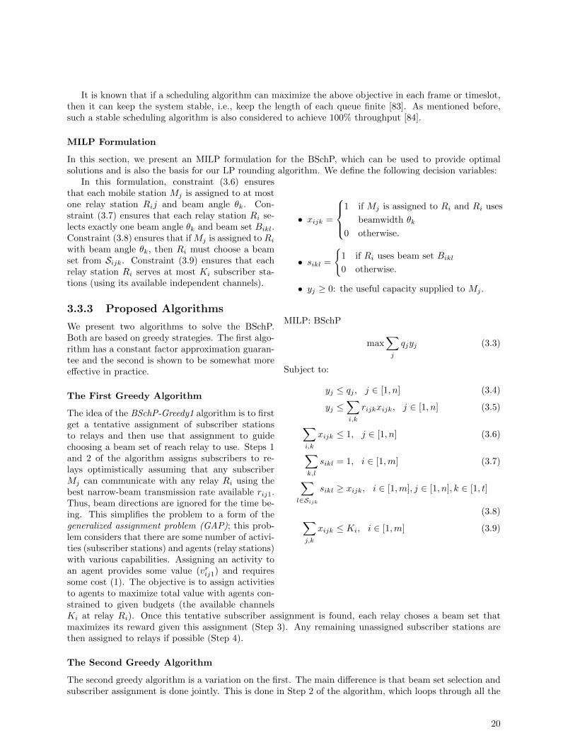
It is known that if a scheduling algorithm can maximize the above objective in each frame or timeslot,then it can keep the system stable, i.e., keep the length of each queue finite [83]. As mentioned before,such a stable scheduling algorithm is also considered to achieve 100% throughput [84].
MILP Formulation
In this section, we present an MILP formulation for the BSchP, which can be used to provide optimalsolutions and is also the basis for our LP rounding algorithm. We define the following decision variables:
• xijk =
1 if Mj is assigned to Ri and Ri uses
beamwidth θk
0 otherwise.
• sikl =
{1 if Ri uses beam set Bikl
0 otherwise.
• yj ≥ 0: the useful capacity supplied to Mj .
MILP: BSchP
max∑j
qjyj (3.3)
Subject to:
yj ≤ qj , j ∈ [1, n] (3.4)
yj ≤∑i,k
rijkxijk, j ∈ [1, n] (3.5)
∑i,k
xijk ≤ 1, j ∈ [1, n] (3.6)
∑k,l
sikl = 1, i ∈ [1,m] (3.7)
∑l∈Sijk
sikl ≥ xijk, i ∈ [1,m], j ∈ [1, n], k ∈ [1, t]
(3.8)∑j,k
xijk ≤ Ki, i ∈ [1,m] (3.9)
In this formulation, constraint (3.6) ensuresthat each mobile station Mj is assigned to at mostone relay station Rij and beam angle θk. Con-straint (3.7) ensures that each relay station Ri se-lects exactly one beam angle θk and beam set Bikl.Constraint (3.8) ensures that if Mj is assigned to Riwith beam angle θk, then Ri must choose a beamset from Sijk. Constraint (3.9) ensures that eachrelay station Ri serves at most Ki subscriber sta-tions (using its available independent channels).
3.3.3 Proposed Algorithms
We present two algorithms to solve the BSchP.Both are based on greedy strategies. The first algo-rithm has a constant factor approximation guaran-tee and the second is shown to be somewhat moreeffective in practice.
The First Greedy Algorithm
The idea of the BSchP-Greedy1 algorithm is to firstget a tentative assignment of subscriber stationsto relays and then use that assignment to guidechoosing a beam set of reach relay to use. Steps 1and 2 of the algorithm assigns subscribers to re-lays optimistically assuming that any subscriberMj can communicate with any relay Ri using thebest narrow-beam transmission rate available rij1.Thus, beam directions are ignored for the time be-ing. This simplifies the problem to a form of thegeneralized assignment problem (GAP); this prob-lem considers that there are some number of activi-ties (subscriber stations) and agents (relay stations)with various capabilities. Assigning an activity toan agent provides some value (vrij1) and requiressome cost (1). The objective is to assign activitiesto agents to maximize total value with agents con-strained to given budgets (the available channelsKi at relay Ri). Once this tentative subscriber assignment is found, each relay choses a beam set thatmaximizes its reward given this assignment (Step 3). Any remaining unassigned subscriber stations arethen assigned to relays if possible (Step 4).
The Second Greedy Algorithm
The second greedy algorithm is a variation on the first. The main difference is that beam set selection andsubscriber assignment is done jointly. This is done in Step 2 of the algorithm, which loops through all the
20

relays and for each, chooses the best beam set to use given the previously made subscriber assignments.Once a beam set is chose for a relay Ri then up to Ki subscribers are assigned to that relay and the loopcontinues.
3.3.4 Simulation Results
In this section, we present simulation results to show the performance of the proposed algorithms. TheILOG CPLEX [85] optimization software was used to solve all the MILP and LP problems. In the simula-tion, n SSs were randomly deployed within a square l× l km region, with a single BS placed at the centerof the square. Then, m RSs were deployed radially from the center of the region with uniform angularspacing and random radii between zero and the maximum distance. In the simulation, we calculated SNRsusing the free space path loss model [80] as described in Section 3.3.1. The transmitter antenna gain ofeach node was set to 360
θ Go, where Go is the gain of an antenna working in the omni-directional mode. Inaddition, each node was assumed to be able to receive signals from all directions, i.e., the receiver antennagain of each node was set to Go. The values of those parameters relevant to the propagation model andother related parameters were set according to Table 3.2.
Table 3.2: Common Simulation SettingsOmni-directional antenna gain Go 2dB;
Operating frequency 5.8GHz;Path loss exponent 2;
Transmit power of each RS (Pt) 1W;Noise power −174dBm/Hz;
Channel bandwidth 10MHz;
As described before, the link capacity is given by a discrete step increasing function. A set of SNRthresholds, and the corresponding modulation indices and link capacities specified by IEEE 802.16e [81]are given in Table 3.3.
Table 3.3: SNR VS. Link CapacitySNR Threshold (dB) Modulation Index Link Capacity (Mbps)
10 QPSK 1/2 1014.5 16QAM1/2 2017.25 16QAM 3/4 3021.75 64QAM 2/3 40
23 64QAM 3/4 45
To simplify the scenarios, we just considered that each RS could use either the beamwidth θ or thebeamwidth 2θ. In each simulations scenario, we changed the value of one parameter and fixed the valuesof the others. We evaluated the performance of the proposed algorithms, i.e., the LP rounding algorithm(labeled as “LP Rounding”) and the greedy algorithm (labeled as “Greedy”), in terms of the total BSchPobjective function, (3.3). In all scenarios, we also computed optimal solutions given by solving the MILPfor the BSchP (labeled as “Optimal”). We summarize our simulation scenarios in the following and presentthe corresponding simulation results in Figs. 3.8–3.12. Each number in these figures is an average over 10runs, each with a different randomly generated network.
• Scenario 1: Vary n, the number of subscribers, in the range {20, 30, 40, 50, 60}.
• Scenario 2: Vary m, the number of relay stations, in the range {6, 8, 10, 12, 14}.
• Scenario 3: Vary θ, the minimum beam angle, in the range {20, 30, 40, 50, 60}. We assume that eachrelay station has angles θ and 2θ available.
21

Figure 3.8: Scenario 1: Performance VS. thenumber of SSs (n)
Figure 3.9: Scenario 2: Performance VS. thenumber of RSs (m)
Figure 3.10: Scenario 3: Performance VS.beamwidth (θ)
Figure 3.11: Scenario 4: Performance VS. meanqueue length (µ)
Figure 3.12: Scenario 5: Performance VS. regionside length (l)
Figure 3.13: Scenario 6: Performance VS. chan-nels per relay (K)
22

• Scenario 4: Vary µ, the mean subscriber queue length, in the range {20, 30, 40, 50, 60} kb. We assumethat each queue length q is drawn from the uniform distribution on [0, 2µ].
• Scenario 5: Vary l, the side length of the l by l simulation region, in the range {20, 30, 40, 50, 60} km.
• Scenario 6: Vary K, the number of independent channels available per relay, in the range {2, 3, 4, 5, 6}.
All non-varying values were set to the median value in their respective range.We make the following observations from simulation results, noting that overall the BSchP-Greedy2
algorithm closely tracks the optimal solution in almost all cases, while the BSchP-Greedy1 algorithmperforms less well in all cases:
1) From Fig. 3.8, we see the BSchP-Greedy2 algorithm performs within 15% of the optimal solution forall cases while the BSchP-Greedy1 algorithm quickly degrades to less than 75% of the optimal.
2) Comparing Figs. 3.9, 3.11 & 3.12 vs. Figs. 3.8, 3.10 & 3.13 we see that the performance of the theproposed algorithms, specifically BSchP-Greedy1 is significantly impacted by the number of subscribers,width of the beam, and number of channels whereas BSchP-Greedy2 is affected the greatest by the widthof the beam, making it much more robust.
3) From Fig. 3.12 & 3.13 we see that as the region size increases and the number of channels increasesbeyond 5 the effectiveness of beam scheduling is reduced reinforcing the fact that beam scheduling is mosteffective for denser networks with a limited number of channels.
3.3.5 Conclusions
In this paper, we have studied the beam scheduling problem for efficient communications in wireless relaynetworks with smart antennas. The corresponding optimization problem was formally defined as the BSchPand was shown to be NP-hard. We first presented a MILP formulation to provide optimal solutions. Thenwe presented two simple and fast localized greedy approachs for BSchP, one of which was shown to havean approximation ratio of 1
2d2πθ1e .
It has been shown by extensive simulation results that the proposed algorithms provide performancebetter than 80% of optimal.
3.4 Channel Selection and Joint Routing and Channel Selectionin Cognitive Radio Networks
This paper was co-authored with Drs. Mumey and Tang, and David Stearns. It has been submitted toInfoComm 2012 and is under review.
Wireless Mesh Networks (WMNs) are considered an economical method of providing robust, high-speed backbone infrastructure and broadband Internet access in large areas [86]. Mesh topology offers theadvantages of alternative route selection to assure throughput and Quality of Service (QoS) requirementsunder dynamic load conditions. As aggregate traffic volume can be substantial on backbone links convergingon gateways and mesh routers, considerations of transmission path routing and how to select channelsalong the path are essential to assure that a WMN can meet the QoS and throughput requirements ofend-users’ applications, especially real-time multimedia applications. Furthermore, range considerationsand propagation characteristics demand careful attention to interference. Cognitive radios are desirable fora WMN in which a large volume of traffic is expected to be delivered since they are able to utilize availablespectrum more efficiently than conventional, static channel assignment methods and therefore improvenetwork capacity significantly [87]. However, they introduce additional complexities to resource allocation.With cognitive radios, each node can access a set of available spectrum bands which may span a widerange of frequencies. Each spectrum band may be divided into channels, and the channel bandwidths mayvary from band to band. Different channels may be able to support quite different transmission ranges anddata rates, both of which have a significant impact on resource allocation and interference effects. Eachnetwork link has some subset of channels available due to the activities of primary users and other trafficin the network.
23

In this paper, we study two hard resource allocation problems in cognitive radio mesh networks: theChannel Selection (CS) problem which is to choose a set of available channels on each link in a givenrouting path so as to maximize end-to-end throughput of the path, and the Joint Routing and ChannelSelection (JRCS) problem where the routing path is not provided as part of the input and must be foundalong with a channel selection for each link on the path. We use a general and accurate approach toestimate end-to-end throughput of a path, in which channel capacities and availabilities are link specific.Our objective is to design efficient approaches to support emerging wireless applications demanding long-standing connections and high end-to-end throughput, such as real-time streaming video or bulk datatransfer. This work is different from some previous works on scheduling and spectrum allocation [37,44, 57–60] which usually dealt with the problem of scheduling and allocating channels to links for link-layer throughput maximization. Here, we focus on end-to-end performance, and consider the problem ofallocating channels along a multi-hop routing path, which is a much harder problem due to the constraintsrelated to intra-flow interference [88] (links on a common path interfere with each other if assigned thesame channels) and due to the fact that in general there are an exponential number of potential paths in amesh network connecting a pair of nodes as well as an exponential number of ways to assign channels alonga path. In addition, the algorithms proposed for traditional WMNs with homogeneous channels [36,69,70]cannot be applied to solve our problems here which target at a large number of heterogeneous channelsthat can support different data rates and transmission ranges. In short, routing and channel selection incognitive radio mesh networks are very challenging problems, which is why most existing works [61–67] onthis topic presented heuristic algorithms that cannot provide any performance guarantees. In this work,we study the CS problem and the JRCS problem from a theoretical perspective and aim at developingtheoretically well-founded and practically useful algorithms to solve them. Our major contributions aresummarized as follows:
1. We present a new characterization of optimal CS solutions, which leads to an efficient dynamic program-ming algorithm that can optimally solve the CS problem, and if the path satisfies a certain naturalself-avoiding criteria (defined in Section 3.4.1), in time linear in the length (hop-count) of the path. Inaddition, the algorithm can be easily implemented in a distributed fashion and an optimal solution canbe computed in a single pass by the nodes along the path with only local information sharing.
2. We also examine the much harder problem of JRCS. We show that obtaining a (2/3 + ε) approximationto the JRCS problem is NP-hard for any ε > 0, which places the JRCS problem in the complexity classof APX-hard. Despite the theoretical hardness, we present two heuristic algorithms to solve the jointproblem.
3. Extensive simulation results show that the proposed joint algorithms outperform the approach using ouroptimal CS algorithm on shortest (minimum hop-count) paths .
The differences between this work and these related works are summarized as follows: (1) In both ofour problems, the objective is to maximize end-to-end throughput, which is different from those worksaddressing link layer (single-hop) throughput such as [37, 44, 57–60]. (2) We obtain an optimal algorithmfor the CS problem, that runs in time linear in the length of the given routing path, provided the pathsatisfies a natural condition. Many related works (such as [61–67]) only presented heuristic algorithms thatcannot provide any performance guarantees. (3) Our optimization problems are different from those studiedin [61–68]. (4) As described above, the algorithms proposed for traditional WMNs with homogeneouschannels [36, 69, 70] cannot be applied to solve our problems here due to channel heterogeneity. (5) Tothe best of our knowledge, we are the first to establish a bound on the complexity of the JRCS problem.We show that it is NP-hard to approximate to within a factor (2/3 + ε) and provide effective heuristicalgorithms to solve it.
3.4.1 Problem Formulation
We consider a wireless mesh backbone network G = (V,E) with static mesh routers, where V is the setof nodes and E is the set of available communications links between the nodes. Each node is equippedwith a cognitive radio. Similar as in [61, 63, 67], a spectrum occupancy map is assumed to be available tonetwork nodes from a centrally-maintained spectrum database. This scenario has recently been promotedby the FCC to indicate over time and space the channel availabilities in the spectrum below 900 MHz and
24

around 3 GHz [41]. In this case, spectrum (channel) availability between any given node pair is known. Westudy the problem of determining the optimal route and channel assignment for a communication sessionbetween two nodes in the network. Spectrum sensing is out of scope of this work.
We define our assumptions about the parameters of the cognitive radio network: Let m be the number ofchannels available in the network. In general, each link e will have only a subset of these channels availableat any given time. This can be due to interference, the link distance being greater than the transmissionrange, or that channel being already in use on that link. We will also assume that each available channelj on link e has an associated bit rate be,j ≥ 0. This bit rate can depend on the link distance and otherfactors. We assume that communication in the network is done using synchronized transmission frames.Let Ae be the set of channels available to link e during the current frame.
We adopt the following simple interference model: We assume that there is an interference distance Rjfor each channel j such that a link e = (u, v) interferes with another link e′ = (u′, v′) on channel j if andonly if |u−v′| ≤ Rj or |u′−v| ≤ Rj . We will also consider that the nodes in question are half-duplex. Thismeans that nodes cannot simultaneously transmit and receive. The duplexing and interference constraintsimpose conditions on which link flows can be active at the same time. We will summarize these conditionsin a well-known conflict graph, Gc = (Vc, Ec), where the vertices Vc are the link-channel pairs (e, j) andthe edges (undirected) indicate those link-channel pairs which cannot be simultaneously operational dueto interference or duplexing constraints.
Suppose we have a routing path p from s to t and a set of active channels Je ⊂ Ae has been chosen to
be used for each link e ∈ p. Let G〈Je〉c,p be the conflict graph restricted to the link-channel pairs of the form
(e, j) where e ∈ p and j ∈ Je. Let te,j be the total amount of time allocated to the link-channel pair (e, j)
in the transmission frame (assumed to be of length 1). Each clique C in G〈Je〉c,p imposes the constraint∑
(e,j)∈C
te,j ≤ 1. (3.10)
Let m〈Je〉e,j be the size of the largest clique containing (e, j) in G
〈Je〉c,p . We make a simplifying assumption
that the scheduling mechanism creates a uniform schedule such that
te,j = 1/m〈Je〉e,j . (3.11)
Observe that each constraint of the form (3.10) is satisfied by (3.11). We note that a uniform schedulemay not be optimal but we adopt this assumption for algorithmic convenience and because it may not bepossible to alter the scheduling mechanism used in a real network.
Let Gjc,p be the subgraph of Gc,p consisting of the link-channel pairs that use channel j.
Definition 2. We say that the routing path p is self-avoiding if all of the subgraphs Gjc,p are intervalgraphs such that the intervals occur in order of p.
This means that the link-pairs in p involving channel j can be placed in order on the real number lineR such that two links-pairs (e, j) and (e′, j) conflict if and only if their corresponding intervals overlap.Interval graphs have a useful property that their cliques can be easily enumerated since a cliques will berepresented by a set of consecutive intervals that all mutually overlap. In fact, all maximal cliques on aninterval graph with n vertices can be enumerated in O(n) time. We will focus on self-avoiding routingpaths in this work because it is easy to find the maximal cliques in their interference graphs.
We define the end-to-end throughput τ of the path p and selected active channels 〈Je〉e∈p, as theminimum over all the links e ∈ p of the effective throughput on link e. The effective throughput of an linke is sum of the bit rates on each active channel times the amount of transmission time allocated to eachchannel,
τ(p, 〈Je〉) = mine∈p
∑j∈Je
be,j/m〈Je〉e,j . (3.12)
We can now formalize the two computational problems considered. In addition to the source node sand destination node t, we assume the available channel sets Ae and bit rates be,j are provided in the input.
Channel Selection (CS): Given a routing path p from s to t, determine active channels sets Je ⊂ Ae forall e ∈ p that maximize the end-to-end throughput τ(p, 〈Je〉).
25
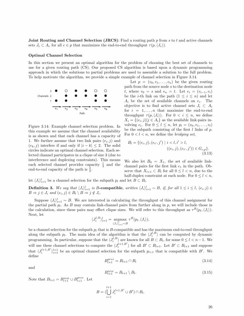
Joint Routing and Channel Selection (JRCS): Find a routing path p from s to t and active channelssets Je ⊂ Ae for all e ∈ p that maximizes the end-to-end throughput τ(p, 〈Je〉).
Optimal Channel Selection
In this section we present an optimal algorithm for the problem of choosing the best set of channels touse for a given routing path (CS). Our proposed CS algorithm is based upon a dynamic programmingapproach in which the solutions to partial problems are used to assemble a solution to the full problem.To help motivate the algorithm, we provide a simple example of channel selection in Figure 3.14.
e1
Channels:
e2 e3 e4 e5
Path
3
2
1
e6
Figure 3.14: Example channel selection problem. Inthis example we assume that the channel availabilityis as shown and that each channel has a capacity of1. We further assume that two link pairs (ei, j) and(ek, j) interfere if and only if |i − k| ≤ 2. The solidcircles indicate an optimal channel selection. Each se-lected channel participates in a clique of size 3 (due tointerference and duplexing constraints). This meanseach selected channel provides capacity 1
3 and theend-to-end capacity of the path is 2
3 .
Let p = (v0, v1, . . . , vn) be the given routingpath from the source node s to the destination nodet, where v0 = s and vn = t. Let ei = (vi−1, vi)be the i-th link on the path (1 ≤ i ≤ n) and letAi be the set of available channels on ei. Theobjective is to find active channel sets Ji ⊂ Aifor i = 1, . . . , n that maximize the end-to-endthroughput τ(p, 〈Ji〉). For 0 < i ≤ n, we defineXi = {(ei, j)|j ∈ Ai} as the available link-pairs in-volving ei. For 0 ≤ l ≤ n, let pl = (v0, v1, . . . , vl)be the subpath consisting of the first l links of p.For 0 < l < n, we define the bridging set,
Bl = {(ei, j), (ei′ , j′) | i < l, i′ > l,
((ei, j), (ei′ , j′)) ∈ Gc,p}.
(3.13)
We also let B0 = X1, the set of available link-channel pairs for the first link e1 in the path. Ob-serve that Xl+1 ⊂ Bl for all 0 ≤ l < n, due to thehalf-duplex constraint at each node. For 0 ≤ l < n,
let 〈Ji〉li=1 be a channel selection for the subpath pl and let B ⊂ Bl.
Definition 3. We say that 〈Ji〉li=1 is B-compatible, written 〈Ji〉li=1 ∼ B, if, for all 1 ≤ i ≤ l, (ei, j) ∈B ⇒ j ∈ Ji and (ei, j) ∈ Bl \B ⇒ j /∈ Ji.
Suppose 〈Ji〉li=1 ∼ B. We are interested in calculating the throughput of this channel assignment forthe partial path pl. As B may contain link-channel pairs from further along in p, we will include those inthe calculation, since these pairs may effect clique sizes. We will refer to this throughput as τB(pl, 〈Ji〉).Next, let
〈J l,Bi 〉li=1 = argmax
〈Ji〉li=1∼BτB(pl, 〈Ji〉),
be a channel selection for the subpath pl that is B-compatible and has the maximum end-to-end throughputalong the subpath pl. The main idea of the algorithm is that the 〈J l,Bi 〉 can be computed by dynamic
programming. In particular, suppose that the 〈J l,Bi 〉 are known for all B ⊂ Bl, for some 0 ≤ l < n− 1. We
will use these channel selections to compute the 〈J l+1,B′
i 〉 for all B′ ⊂ Bl+1. Let B′ ⊂ Bl+1 and suppose
that 〈J l+1,B′
i 〉l+1i=1 be an optimal channel selection for the subpath pl+1 that is compatible with B′. We
defineBprevl+1 = Bl+1 ∩Bl (3.14)
andBnewl+1 = Bl+1 \Bl. (3.15)
Note that Bl+1 = Bnewl+1 ∪Bprevl+1 . Let
B = (
l+1⋃i=1
J l+1,B′
i ∪B′) ∩Bl.
26

We observe that B ⊂ Bl and that B agrees with B′ on Bprevl+1 (this means B ∩Bprevl+1 = B′ ∩Bprevl+1 ). Thus,
τB′(pl, 〈J l+1,B′
i 〉li=1) = τB(pl, 〈J l+1,B′
i 〉li=1)
≤ τB(pl, 〈J l,Bi 〉li=1), (3.16)
since the throughput on all of the links in the subpath pl is unchanged. We use the notation, m〈Jl+1,B′
〉,B′
el+1,j
to refer to the size of the largest clique containing (el+1, j) present among the link-channel pairs from〈J l+1,B′〉 and B′ together. Let
< Jopt >= 〈J l,B〉, J l+1,B′
l+1 ;
the channel assignments given by 〈J l,B〉 for the subpath pl and by J l+1,B′
l+1 for link el+1. A key observation
is that m〈Jl+1,B′
〉,B′
el+1,j= m
〈Jopt〉,B′
el+1,jfor any (el+1, j) ∈ J l+1,B′
l+1 since both Bi and Bi+1 will contain anylink-channel pairs from pl+1 that conflict with it. We have,
τB′(pl+1, 〈J l+1,B′
〉)
= min(τB(pl, 〈J l+1,B′〉li=1),∑
j∈Jl+1,B′l+1
bel+1,j/m〈Jl+1,B′
〉,B′
el+1,j)
≤ min(τB(pl, 〈J l,B〉li=1),∑j∈Jl+1,B′
l+1
bel+1,j/m〈Jopt〉,B′
el+1,j)
= τB′(pl+1, 〈Jopt〉). (3.17)
Since 〈J l+1,B′〉 was assumed optimal, we must have equality in (3.17), so we can take
〈J l+1,B′〉 = 〈Jopt〉. (3.18)
Equation (3.17) shows that the optimal channel selection for pl+1 and B′ can be expressed in terms ofan optimal channel selection for pl and B, a smaller problem. This means that we can use dynamicprogramming to compute 〈J l+1,B′〉. The idea is to take each 〈J l,B〉 found for pl and extend to channelassignment for pl+1 for all B′ ⊂ Bl+1 such that B and B′ agree on Bprevl+1 . Since B fixes which link-pairs from Bprevl+1 are included in B′, we can simply enumerate all subsets B′′ ⊂ Bnewl+1 and for each, formB′ = (B ∩ Bprevl+1 ) ∪ B′′. Also, since Xi+1 ⊂ Bi, we let B also determine all channel assignments for linkel+1:
〈J test〉 = 〈J l,B〉, (B ∩Xi+1). (3.19)
We then evaluate τB′(pl+1, 〈J test〉) to see if J test provides a better channel assignment for pn+1 compatible
with B′; if yes, we keep it. This evaluation is done in the same fashion as (3.17):
τB′(pl+1, 〈J test〉) = min(τB(pl, 〈J l,B〉li=1)),∑
j∈B∩Xi+1
bel+1,j/m〈Jtest〉,B′
el+1,j) (3.20)
In order to evaluate (3.20), we need to calculate the second min term since the first is already known.This is done by determining the largest clique that (el+1, j) participates in among link-channel pairs from〈J test〉, B′. If we make the assumption that the routing path p is self-avoiding, then any clique in involving(el+1, j) is either a consecutive list of link-channel pairs in Gjc,p (that all mutually overlap in the intervalgraph representation), or a clique involving (el+1, j) and a link-channel pair from Xl or Xl+2 or both, usinga channel other than j. Let ∆ be the maximum degree of any node in any of the Gjc,p and suppose thereare at most mp channels available on any link in p. All of the clique possibilities can be checked in O(∆mp)time, so this is the time required to evaluate (3.20).
27

3.4.2 Proposed Algorithms
In this section we present two heuristic algorithms for the joint problem of routing and channel selection.
A Path Extension Algorithm
The first proposed algorithm is based on the idea of simultaneously finding good path/channel assignmentsfrom the source node s to all other nodes in the network, including the destination node t. The approach issimilar to the Bellman-Ford shortest-path algorithm in that new path/channel assignments are generatedby “relaxing” all the links in the network in a series of phases that continues until no better paths arediscovered. Each node u 6= s will store a list Pu of path/channel assignments of the form (pu, 〈Je〉e∈pu),where pu is a path from s to u. When the link (u, v) is relaxed, the current path/channel assignments storedat u will be augmented by the link (u, v); for each subset J ′ ⊂ A(u,v) we will create a new path/channelassignment (p′v, 〈Je, J ′〉), where p′v is the path pu followed by the link (u, v). To limit the search, eachnode keeps a maximum of d best path/channel assignments (we chose d = 100). We also note that it isonly necessary to augment those path/channel assignments that were created in the previous phase; wewill refer to these as new in the algorithm. Clearly, a loop in a path can never improve the end-to-endthroughput of the path, so we restrict attention to simple paths that never repeat a vertex. We also requirethat the path be self-avoiding.
Bottleneck Routing
The second approach attempts to find a single path whose links all have a high useful capacity. Wemake this precise as follows. We define the link capacity c(e) of a link e as, c(e) =
∑j∈Ae be,j . The link
capacity provides an upper bound on the bit flow rate achievable by link e ignoring intra-path interference.In addition to link capacity, we also take into account how close the link e = (u, v) to the source s anddestination t. For each link e = (u, v), let d(e) = ||u−s||+||u−s||+||v−s||+||v−t||. Let dmax = maxe∈E d(e)and dmin = mine∈E d(e). An heuristic additional weighting factor on the link capacity to better estimatethe usefulness of a link e for an s-t path. We define
u(e) = (1 +dmax − d(e)
dmax − dmin)c(e), (3.21)
and consider the useful bottleneck capacity of a path p to be
c(p) = mine∈p
u(e).
Our goal is to find a path p that maximizes c(p). This is a well-known problem that can be efficientlysolved by computing a minimum spanning tree T on the network graph using an link weight functionw(e) = −u(e). The unique path in T from s to t will have maximum useful bottleneck capacity. We labelthis algorithm RCS-Bottleneck.
3.4.3 Simulation Results
To test our routing and channel selection algorithms we compared it against simple shortest path routingusing Dijkstra’s algorithm (the edge weights in this case were the physical link distances) followed by theDP-ChannelSelect algorithm to find the optimal channel selection for the shortest path. In all cases tried,the DP-ChannelSelect algorithm itself runs in under a second on a laptop computer.
For our experiments, we assumed there were three widely spaced frequency bands available for licensedand unlicensed operation and that the link throughput for each channel was the maximum available giventhe link distance and frequency used. The bands exhibit widely ranging propagation, transmission rangeand usage characteristics, highlighting the potential value of cognition in transmission scheduling. Tables 1and 2 summarize our assumptions about the transmission rates and interference ranges of each frequency.These values are based on a scenario where each node transmits at 1W with a 2dBi antenna and thereceiving antenna has a gain of 2dBi. The channel bandwidth is 10 MHz and the receiver noise figureis 5dB, and implementation losses of 3dB are assumed for each link. Path loss is calculated using line
28

Table 3.4: Maximum transmission distances by frequency and data rateTransmission rate 700 Mhz 2400 Mhz 5800 Mhz
45 Mbps 15.4 km 4.5 km 1.8 km40 Mbps 18.4 km 5.3 km 2.2 km30 Mbps 30 km 8.6 km 3.6 km20 Mbps 41 km 11.8 km 4.9 km10 Mbps 68 km 20 km 8.2 km
Figure 3.15: Average path end-to-end through-put versus the number of available channels.
Figure 3.16: Average path end-to-end through-put versus network size. Node density was heldconstant at 0.01nodes/km2.
of sight and free space characteristics. Typical IEEE 802.16 adaptive modulation and coding parametersperformance parameters were used to estimate the throughput achievable as a function of CNR (carrierto noise ratio), and were then translated into the allowable path loss threshold. The maximum channeltransmission rate is a function of distance and frequency (at lower frequency, the maximum distance fora given transmission rate will be greater). We assumed that each channel was available on each linkwith independent probability 0.5. Primary users were placed at random locations and assigned a randomchannel. This channel was then made unavailable to any links of cognitive radios within the interferencerange of the primary user.
Table 3.5: Interference ranges by frequencyFrequency Interference range700 Mhz 30.8 km2400 Mhz 9 km5800 Mhz 3.6 km
Scenario 1: Varying the number of channels available
In this scenario, the number of channels available to secondary users was varied from 3 to 15 with a stepsize of 3 (chosen equally from each frequency band). Ten random source-destination pairs were generatedon a 50×50km2 network with 25 nodes and 5 primary users. These pairs and the node locations were heldconstant for all of the experiments in this scenario. The average end-to-end transmission rate (throughput)for all routing path and channel selections is reported. The results, shown in Figure 3.15, indicate analmost linear improvement is gained by adding additional channels to the network in terms of additionalthroughput. The path and channel assignments found by the RCS-PathExtend were, on average, 13.23%better than those found by CS-ShortestPath, and 8.67% better than those found by RCS-Bottleneck.
29

Scenario 2: Varying Region Size
In this scenario, the physical region size was increased, but node density was held constant. Ten randomsource-destination pairs were generated on a network with 3 channels per frequency band, 5 primary users,and a constant density of 0.01nodes/km2. The average end-to-end transmission rate for all routing pathand channel selections is reported. As the region size grows, paths tend to get longer. The results, shownin Figure 3.16, indicate that the RCS-PathExtend algorithm continues to outperform the two other routingand channel assignment methods and that gap increases slightly as the region size increases. The path andchannels assignments found by the RCS-PathExtend algorithm were, on average, 9.97% better than thosefound by CS-ShortestPath, and 20.46% better than those found by RCS-Bottleneck.
Scenario 3: Varying Node Density
Figure 3.17: Average path end-to-end through-put versus node density. Region size fixed to50× 50km2.
In this scenario, the physical region size was held con-stant at 50 × 50km2 and the number of nodes was in-creased. Ten random source-destination pairs were gen-erated on a network with 3 channels per frequency band,5 primary users. The average end-to-end transmissionrate for all routing path and channel assignments is re-ported. As the network size grows, node density in-creases and the average number of links that a given linkinterferes with on a given channel increases. The effectis to increase the average vertex degree in the conflictgraph Gc. The results, shown in Figure 3.17, indicatethat again, the RCS-PathExtend algorithm outperformsthe two other approaches across the range of node den-sities considered. That path and channel assignmentsfound by the RCS-PathExtend algorithm were, on aver-age, 8.26% better than those found by CS-ShortestPath,and 11.52% better than those found by RCS-Bottleneck.
3.4.4 Conclusions
In this paper, we have examined two important problemsfor maximizing the end-to-end throughput for communi-cation flows in cognitive radio mesh networks. For thechannel selection problem on a known routing path, we developed an optimal algorithm and showed thatfor self-avoiding paths it runs in time linear in the length of the path. Furthermore, the algorithms onlyneeds to propagate local information from source to destination and can be implemented in a distributedfashion. We also considered the joint problem of routing and channel selection and showed that it was NP-hard to approximate within a factor of (2/3 + ε). In addition we presented two novel heuristic algorithmsfor this problem and demonstrated the universal superiority of one of them, RCS-PathExtend, to simplyusing shortest path routing followed by optimal channel selection.
30

Chapter 4
Research Plan
Presented here is the plan for my research which is composed of two pieces: extending my previous work toaccount for topography and whitespace frequencies, enhance a sparse broadband network architecture withtopology control and game theoretic algorithms to overcome challenges to connectivity and throughput insparseness challenges in rural wireless network implementations. These two problems address the greatestchallenges in providing a robust and cost-effective solution for rural wireless networking. As my researchprogresses it will evolve and adapt, and this plan will evolve accordingly.
4.1 Research Goals
The goal of my research is to produce an architecture with enhancements based on a set of algorithms, anda set of possible technologies (radios, frequencies, antennas, power systems) that can be used to implementsparse wireless networks where node distribution is non-uniform. To accomplish this goal we need toinvestigate the effects of that topography and expanded frequency spaces have on beam selection, beamscheduling and routing and channel selection. Additionally I want to verify that the existing wirelessarchitecture deployed as part of the Buffalo Jump Technology Cooperative is the best general solution. Ialso want to provide enhancements that improve connectivity robustness by by avoiding single points offailure in the existing solution.
The existing wireless networking data and simulations are severely limited in their usefulness for ex-tracting meaningful information about the connectivity (or lack thereof) among rural parts of America. Ibelieve more measurement and simulation can significantly improve the data about existing connectivityand illuminate the most cost effective way to connect the rest of America. One of my goals is to show thatby enhancing simulations to three dimensions and expanding the frequency range to include TV whitespacesolutions are feasible to enfranchise a significant amount of the remaining disconnected Americans.
The second goal of my research is to show that a sparse broadband network architecture can be builtusing topology control to provide a robust long range wireless backbone connecting wireless meshes is ageneral solution to the extending broadband infrastructure to reach remote users in areas with low popu-lation density, highly varying topography or both. The artifacts of my research will include publications,a simulation toolkit, and an in situ wireless testbed.
4.2 Extensions to Current Work
4.2.1 Topography
In order to account for topographical considerations there are two additional factors that need to beadded to the existing simulations. First, the simulations need to take elevation into account adding someadditional computational complexity in the distance, range, and throughput computations. The additionof elevation takes the simulations from 2D to 3D, which makes them both more accurate and more realistic.
31

Second, natural topography also provides signal blocking that needs to be taken into account. This signalblocking significantly alters the routing and frequency selection components of the simulation.
In order to realistically simulate wireless networking implementations both of these factors need to beincorporated, resulting in updated papers for beam scheduling, beam selection and routing and channelselection. These updated papers will submitted to conferences for publication.
4.2.2 Whitespace
Additionally, with the recent moves to make TV whitespace frequencies available, and since these fre-quencies are in the range that can provide long range connectivity, I plan to enhance the simulations toinclude the ability to use TV whitespace frequencies. The addition of these frequencies could improve theperformance of the simulation by providing longer range more topographically robust link options.
Again, updated publications will be produced and submitted to relevant conferences. Depending uponthe outcome of the simulations the publications might combine the topographical awareness and extendedfrequency ranges into a single set of publications.
4.2.3 Beam Refinement
An additional problem that I am pursuing involves finding the optimal beam selection when given atransmission schedule. This comes from a problem in WiMAX networks where the two phase process ofidentifying nodes and scheduling the transmission via separate sub-channels provides the possibility of amulti-sector antenna to focus activate and deactivate sectors for each sub-channel in sequence. This couldprovide significantly more transmission power by focusing the power in the direction of the transmission foreach time slice. This would require sniffing the transmission schedule packets from the WiMAX networkusing a protocol analyzer and solving the beam scheduling problem fast enough to activate antenna sectorsfor each transmission.
4.3 Future Work
All of the new work I propose is based on a wireless architecture that is made up of one or more internetgateways, a set of relay nodes and a set of subscriber nodes. The internet gateways and relay nodes providethe network backbone and are assumed to span long distances using TVWS. This subnetwork uses topologycontrol mechanisms to maximize connectivity and throughput while minimizing interference. Subsets ofone or more subscriber nodes in this network compose wireless mesh clouds, providing high bandwidthconnectivity to each other. The link between these subscriber clouds and the backbone is a set of cognitiveradio enhanced subscriber nodes that are periodically elected to be relay nodes routing traffic to and fromthe backbone. This network architecture could address the greatest resource issues that occur in sparsenetworks where node distribution uniformity is unknown a priori.
4.3.1 A Sparse Broadband Network Architecture
The network architecture I propose is a topology control backbone network connecting wireless meshsubnetworks. The hardware can be uniform or non-uniform as long as there are at least two cognitiveradios with the same frequency capabilities as the relay nodes that connect the meshes. Referring backto Fig. 3.7, each of the subscriber stations (SS) and their associated relay station (RS) are a traditionalwireless network, each with the capability of being the RS. There can be more RS’s in the network thatare not part of local wireless networks, providing traditional RS services as well. Each wireless cloud electsa set of one or more RS’s to provide gateway services to the upper layer network of RS’s that in turn routetraffic through the set of internet gateways. The election of RS’s within wireless networks can happen ata fixed interval or be in response to changing network conditions induced by changes in weather, usage,or hardware performance. This re-election of RS’s triggers a topology control event where the upper layercan re-evaluate the topology control solution for the routing network to ensure optimal performance. Theupper layer topology control network can also have a cognitive trigger with an interval to re-evaluate the
32

topology control solution providing routing among existing (e.g. non-changing) RS’s. This will have anexponential back-off integrated to avoid any loss in performance when conditions are not changing rapidly.
There are multiple aspects of this architecture that can be explored to provide the optimal implementa-tion. Here I describe the various components of the architecture. Each of these is a possible improvementin the basic sparse broadband network architecture composed of 2.4GHz/900MHz nodes that are in placeas part of the Buffalo Jump Technology Cooperative.
Topology Control Backbone Network
The topology control based routing network that provides the backbone of the architecture is characterizedby the distances and topographical challenges it needs to overcome. In sparse networks, links in the routingnetwork span long distances, from 5 to 50 miles, at these distances exercising MAC layer modifications andextended ACK timeout techniques is sufficient, however, failure is possible and the routing network stillneeds multiple paths to ensure durable connectivity and maximize throughput. Extending the cognitiveradios in this layer with the ability to use more frequencies provides more robust, long distance network linksif they are at lower frequencies — such as the TV whitespace. This routing network is ideally composedof narrow beam point-to-point or point-to-multipoint connections that can focus on other relays stationswhether they are fixed as part of the routing network or changing in the subscriber clouds.
The advantages of this narrow beam, mostly fixed routing network which is dynamically reconfiguringitself to provide durable connectivity and optimum throughput come from the fact that it’s a fixed infras-tructure that can be deployed and configured in locations where access is limited. It is constrained onlyby the availability of power. Most of the locations where the RS’s need to be located are higher locationswhere access is limited or not possible for the months of December through March.
• Topology Control
Using a topology control approach for the backbone super network pre-computes an antenna patternfor each node such that a certain network topology can be formed for future communications. Thisapproach is used to optimize frequency resources when scarce. Typical scarcity in frequency resourcesis due to over utilization in areas of high population density, however frequency resources can also bescarce when they are not able to be used by more than one pair of radios at a time – such as in TVWSwhere more than one pair of communicating nodes would significantly degrade the performance of thenetwork link. I propose to investigate how many TVWS frequencies are required and what the timingconstraints are on frequency switching times. Traditionally Topology Control algorithms use antennabeam switching, but I propose to use TVWS frequency switching to investigate the complexity andconstraints of using TVWS frequencies for sparse network links. Compared to the alternative cross-layer approach, the major advantage to using the topology control approach is that it is purely a linklayer solution that does not require any modifications to a standard MAC protocol. Hence, it canbe easily implemented in a system using Commercial-Off-The-Shelf (COTS) and standard protocols.This makes it ideal for the existing testbed.
• Whitespace Frequencies
Expanding the available frequencies to include recently freed up TV whitespace can significantly en-hance the Topology Control Backbone Network by allowing the links to span much greater distances.Whitespace frequencies with longer wavelengths, provide the ability to transmit and receive overgreat distances, over obstacles, and through most objects that can cause interference with the shorterwavelengths of higher frequency communications systems. Although the bandwidths are lower ingeneral radio communications at the lower frequencies in the TV whitespace region are robust, asevidenced by multiple decades of success of Television. Multiple lower frequencies could be used inparallel to improve overall performance of the long distance links when needed. The use of whitespacefrequencies in sparse networks is ideal because the correlation of TV whitespace and low populationdensity is intuitively obvious, confirmed by my tests, reports from the FCC and other independentsources.
Using a single 6MHz channel the approximate maximum throughput is 19Mbps with a maximumrange of 30km. To provide sufficient bandwidth for current usage multiple channels will need to be
33

used together, thus the emerging 802.22 specifications assume multiple channels will be bonded tobehave as a single network link. The 802.22 specifications [16] also assume the MAC layer assumescognitive radios to do spectrum sensing — to provide the ability to sense what channels are beingused and what are available. This sensing is necessary to avoid multiple radios using the same TVWSfrequency causing interference and degraded performance on that channel.
• Topographic Issues
Topographical issues need to be taken into account in the proposed network architecture and willbecome obvious in the topology of the backbone network. The overall wireless network will be seg-mented into smaller wireless mesh networks because of distance, but primarily because of topograph-ical features that interrupt higher frequency communication systems. The purpose of integratingtopographical awareness into the simulation toolkit is to provide more precise planning and analysistools and verify them against the existing wireless BJTC wireless network.
Distributed Segmented Smart Mesh Layer
• Basic WDS Clouds extended with Cognitive Radios
The basic implementation of the proposed network architecture involves building each layer usingcognitive radios enabled with extended frequency ranges that include the TV whitespace frequencies.This solution can be immediately realized with commercial off-the-shelf (COTS) hardware, with stan-dard frequencies (900MHz, 2.4GHz, and 5.8 GHz) and then be extended with devices that can takeadvantage of the lower frequencies in the TV space. This staged implementation provides an initialbaseline implementation that allows for gathering data on the required hardware for deployment,connectivity, bandwidth, and usage. And then an extension to it into the TV Whitespace where thesame data can be collected again for comparison. This initial COTS implementation also providesthe data necessary to identify any architectural issues or components that will be prone to failureor underperformance. Then those architectural components can be investigated further based on myproposed solutions using topology control and game theory.
Currently, the BJTC wireless network is composed of a 2.4GHz cloud in the lower Madison Valley,connected to Table Mountain where there is a 900MHz link to Three Forks, MT where the internetgateway is. There is also another 5.8GHz network that comes from Bull Mountain to Table Mountain,continues to Pony, MT then on to Whitehall, MT. I am in discussions with the connecting all of thenodes with various antenna’s optimized for coverage and distance, respectively. Since the cost ofradios and antennas is about equivalent and some radios are able to us more than one antenna, thisimplementation can be further optimized with little cost. The next phase of the implementation isto replace the link from the internet gateway to table mountain with a 900MHz point-to-point link.After that a a third 900MHz node will be deployed on the eastern side of the Madison Valley, justsouth of the Madison Buffalo Jump State Park. These three 900MHz nodes are accompanied by2.4GHz nodes that provide connectivity to the wireless mesh on the valley floor.
• Game Theoretic Election of Relay Node(s)
The critical links in the proposed architecture are the relay nodes that gateway between the localwireless networks and the backbone, providing access to other wireless networks and the internet. Inorder to create a robust, fault tolerant architecture one or more of these relay nodes must be allowedto fail without losing overall connectivity. This requirement will drive the need to deploy redundanthardware, which will increase cost. Therefore this requirement is a cost minimization problem wherethe most important constraint is no loss of connectivity given the failure of a maximum number ofnodes.
In order to accomplish this I propose that all nodes in the wireless cloud with visibility to any nodeoutside of the cloud be identified as possible relays. Then using a game theoretic approach – onewhere each node makes configuration and routing choices in a selfish way – the wireless cloud canreconfigure itself to provide one or more relays at any time, maximizing throughput and guaranteeingconnectivity. In order for this solution to work it is required there are at a minimum two nodes in
34
the wireless network that can be relays at any given time. This technique is robust in the face oflimited resources and in a rural network the resources are constantly changing in response to weather,foliage, and transient interfering signals. Additionally, because of the distances and varying terraintopographical constraints limit the fresnel zones of the wireless signal making entirely interferencefree signals too costly to consider. These limitations of the network topology create constraints thatthe game theoretic approach can adapt to and compensate for by through dynamic reconfiguration.
4.4 Timeline
Below is an estimated plan for my research. This plan will certainly evolve as new ideas emerge. Includedbelow are the anticipated publications produced, which will be submitted to peer-reviewed conferences orjournals to report on my results. My goal is 2-5 more papers submitted by March 2012.
• September 2011: Topographical Enhancements to existing Simulations (3 extended papers)
• October 2011: Frequency Enhancements to existing Simulations (3 extended papers)
• December 2012: Game Theoretic Relay Selection Simulation(1 new paper)
• February 2012: Sparse Broadband Network Architecture Simulation (1 new paper), begin Ph.D.dissertation
• April 2012: Complete Ph.D. dissertation
• May 2012: Defend Ph.D. dissertation
35

Bibliography
[1] WildBlue, “Wildblue satellite internet service,” http://www.wildblue.net.
[2] HughesWay, “Hughesnet satellite internet service,” http://www.hughesnet.com.
[3] “FCC Report to the US Congress on Advanced Telecommunications.”
[4] NTIA, “Digital nation expanding internet usage,” http://www.ntia.doc.gov/files/ntia/publications/ntia internet use report february 2011.pdf, February 2011.
[5] FCC, “Fcc’s sixth broadband deployment report,” http://transition.fcc.gov/Daily Releases/DailyBusiness/2010/db0720/FCC-10-129A1.pdf.
[6] J. Horrigan, “Home broadband adoption 2009,” Pew Internet & American Life, Washington, DC,USA, 2009.
[7] Z. Mingliu and R. Wolff, “Crossing the digital divide: cost-effective broadband wireless access for ruraland remote areas,” Communications Magazine, vol. 42, 2004.
[8] S. Surana, R. Patra, S. Nedevschi, M. Ramos, L. Subramanian, Y. Ben-David, and E. Brewer, “Be-yond pilots: keeping rural wireless networks alive,” in Proceedings of the 5th USENIX symposium onnetworked systems design and implementation. USENIX Association, 2008, pp. 119–132.
[9] R. Wolff, “Citizen political enfranchisement and information access: Telecommunications services inrural and remote areas,” in Communications Research in Action. Fordham University Press, January2011.
[10] J. Bicket, D. Aguayo, S. Biswas, and R. Morris, “Architecture and evaluation of an unplanned 802.11b mesh network,” in Proceedings of the 11th annual international conference on Mobile computing andnetworking. ACM, 2005, pp. 31–42.
[11] Meraki, “Meraki cloud managed wireless networks,” http://meraki.com.
[12] FrieFunk, “Freifunk: Free open source radio firmware,” http://start.freifunk.net.
[13] C. Palazzi, M. Brunati, and M. Roccetti, “An OpenWRT solution for future wireless homes,” inMultimedia and Expo (ICME), 2010 IEEE International Conference on, 2010, pp. 1701–1706.
[14] R. Patra, S. Nedevschi, S. Surana, A. Sheth, L. Subramanian, and E. Brewer, “Wildnet: Designand implementation of high performance wifi based long distance networks.” NSDI, 2007. [Online].Available: http://www.usenix.org/events/nsdi07/tech/full papers/patra/patra html/
[15] K. Sibanda, H. Muyingi, and N. Mabanza, “Building Wireless Community Networks with 802.16Standard,” in Broadband Communications, Information Technology & Biomedical Applications, 2008Third International Conference on, 2008, pp. 384–388.
[16] C. Stevenson, G. Chouinard, Z. Lei, W. Hu, S. Shellhammer, and W. Caldwell, “Ieee 802.22: The firstcognitive radio wireless regional area networks (wrans) standard,” IEEE Communications Magazine,pp. 130–138, 1 2009, doi:10.1109/MCOM.2009.4752688.
36

[17] IEEE, “Ieee 802 lan/man standards committee 802.22 wg on wrans (wireless regional area networks),”http://www.ieee802.org/22/.
[18] E. Bangeman, “The white spaces coalition’s plans for fast wireless broadband: The technology,”http://arstechnica.com/articles/paedia/hardware/white-space.ars/2, 2007, ars Technica, 2007-4-17.
[19] D. Benyamina and Hafid, “Wireless Mesh Networks Design — A Survey,” Communications Surveys& Tutorials, IEEE, no. 99, pp. 1–12, 2011.
[20] H. Moustafa, U. Javaid, and T. Rasheed, “A panorama on wireless mesh networks: Architectures,applications and technical challenges,” . . . on “Wireless Mesh: . . . .
[21] J. Ishmael, S. Bury, D. Pezaros, and N. Race, “Deploying Rural Community Wireless Mesh Networks,”Internet Computing, IEEE, vol. 12, no. 4, pp. 22–29, 2008.
[22] M. Zhang and R. Wolff, “Using Wi-Fi for cost-effective broadband wireless access in rural and remoteareas,” in Wireless Communications and Networking Conference, 2004. WCNC. 2004 IEEE, 2004,pp. 1347–1352.
[23] W. Almuhtadi, “Rural/Remote WiFi Wireless Broadband System,” in Wireless On-demand NetworkSystems and Services, 2005. WONS 2005. Second Annual Conference on, 2005, pp. 180–188.
[24] D. Johnson, “Evaluation of a single radio rural mesh network in south africa,” Network.
[25] R. Flickenger, S. Okay, E. Pietrosemoli, M. Zennaro, and C. Fonda, “Very long distance wi-fi net-works,” in NSDR ’08: Proceedings of the second ACM SIGCOMM workshop on Networked systemsfor developing regions. ACM, Aug. 2008.
[26] A. Sharma, “FreeMAC: framework for multi-channel mac development on 802.11 hardware,” in Pro-ceedings of the ACM workshop on . . . , 2008.
[27] R. Mahajan, M. Rodrig, D. Wetherall, and J. Zahorjan, “Analyzing the MAC-level behavior of wire-less networks in the wild,” in SIGCOMM ’06: Proceedings of the 2006 conference on Applications,technologies, architectures, and protocols for computer communications. ACM Request Permissions,Aug. 2006.
[28] R. R. Choudhury and N. H. Vaidya, “Deafness: A MAC Problem in Ad Hoc Networks when using Di-rectional Antennas,” in ICNP ’04: Proceedings of the 12th IEEE International Conference on NetworkProtocols. IEEE Computer Society, Oct. 2004.
[29] T. Korakis, G. Jakllari, and L. Tassiulas, “A mac protocol for full exploitation of directional antennasin ad-hoc wireless networks,” in Proceedings of the 4th ACM international symposium on Mobile adhoc networking & computing. ACM, 2003, pp. 98–107.
[30] K. Sundaresan and R. Sivakumar, “A unified mac layer framework for ad-hoc networks with smartantennas,” in Proceedings of the 5th ACM international symposium on Mobile ad hoc networking andcomputing. ACM, 2004, pp. 244–255.
[31] Y. Ben-David, M. Vallentin, S. Fowler, and E. Brewer, “JaldiMAC: taking the distance further,” inNSDR ’10: Proceedings of the 4th ACM Workshop on Networked Systems for Developing Regions.ACM Request Permissions, Jun. 2010.
[32] K. Ramachandran, I. Sheriff, and E. Belding, “A multi-radio 802.11 mesh network architecture,”Mobile Networks and . . . , 2008.
[33] A. Dhananjay, H. Zhang, and J. Li, “Practical, distributed channel assignment and routing in dual-radio mesh networks,” ACM SIGCOMM . . . , 2009.
[34] M. Gerla and K. Tang, “TCP performance in wireless multi-hop networks,” Mobile Computing Systems. . . , 1999.
37

[35] J.-H. Huang, L.-C. Wang, and C.-J. Chang, “Throughput-coverage tradeoff in a scalable wireless meshnetwork,” Journal of Parallel and Distributed Computing, vol. 68, no. 3, Mar. 2008.
[36] J. Tang, G. Xue, and W. Zhang, “Interference-aware topology control and qos routing in multi-channelwireless mesh networks,” in Proceedings of the 6th ACM international symposium on Mobile ad hocnetworking and computing. ACM, 2005, pp. 68–77.
[37] J. Huang, R. Berry, and M. Honig, “Spectrum sharing with distributed interference compensation,”New Frontiers in Dynamic Spectrum Access Networks, 2005. DySPAN 2005. 2005 First IEEE Inter-national Symposium on, pp. 88–93, 2005.
[38] K. Moaveni-Nejad, “Low-interference topology control for wireless ad hoc networks,” Ad Hoc & SensorWireless Networks, 2005.
[39] R. Lotun, “wypy: an extensible, online interference detection tool for wireless networks,” 2008.
[40] D. Gokhale, S. Sen, and K. Chebrolu, “On the feasibility of the link abstraction in (rural) meshnetworks,” INFOCOM 2008 The . . . , 2008.
[41] F. FCC, FCC 08-260. Unlicensed Operation in the TV Broadcast Bands, 2008. [On-line]. Available: http://scholar.google.com/scholar?q=related:5KyINcAbjPsJ:scholar.google.com/&hl=en&num=30&as sdt=0,5
[42] P. Bahl, R. Chandra, T. Moscibroda, R. Murty, and M. Welsh, “White space networking with wi-fi likeconnectivity,” ACM SIGCOMM Computer Communication Review, vol. 39, no. 4, pp. 27–38, 2009.
[43] S. Deb, V. Srinivasan, and R. Maheshwari, “Dynamic spectrum access in DTV whitespaces: designrules, architecture and algorithms,” in MobiCom ’09: Proceedings of the 15th annual internationalconference on Mobile computing and networking. ACM Request Permissions, Sep. 2009.
[44] Y. Yuan, P. Bahl, R. Chandra, T. Moscibroda, and Y. Wu, “Allocating dynamic time-spectrum blocksin cognitive radio networks,” in MobiHoc ’07: Proceedings of the 8th ACM international symposiumon Mobile ad hoc networking and computing. ACM Request Permissions, Sep. 2007.
[45] K. Sundaresan, W. Wang, and S. Eidenbenz, “Algorithmic aspects of communication in ad-hoc net-works with smart antennas,” in Proceedings of the 7th ACM international symposium on Mobile adhoc networking and computing. ACM, 2006, pp. 298–309.
[46] K. Sundaresan, R. Sivakumar, M. Ingram, and T. Chang, “Medium access control in ad hoc net-works with mimo links: optimization considerations and algorithms,” IEEE Transactions on MobileComputing, pp. 350–365, 2004.
[47] B. Mumey, J. Tang, and T. Hahn, “2008 IEEE International Conference on Communications,” in 2008IEEE International Conference on Communications. IEEE, 8, pp. 2921–2925.
[48] M. Hu, “MIMO ad hoc networks: Medium access control, saturation throughput, and optimal hopdistance,” Networks, 2004.
[49] R. Bhatia and L. Li, “Throughput optimization of wireless mesh networks with mimo links,” inINFOCOM 2007. 26th IEEE International Conference on Computer Communications. IEEE. Ieee,2007, pp. 2326–2330.
[50] C. Ang, “iMST: A bandwidth-guaranteed topology control algorithm for TDMA-based ad hoc net-works with sectorized antennas,” Computer networks, 2008.
[51] Z. Huang and C.-C. Shen, “Multibeam Antenna-Based Topology Control with Directional PowerIntensity for Ad Hoc Networks,” IEEE Transactions on Mobile Computing, vol. 5, no. 5, May 2006.
[52] U. Kumar and H. Gupta, “A topology control approach to using directional antennas in wireless meshnetworks,” Communications, 2006.
38

[53] V. Namboodiri, L. Gao, and R. Janaswamy, “Power-efficient topology control for static wireless net-works with switched beam directional antennas,” Ad Hoc Networks, vol. 6, no. 2, Apr. 2008.
[54] A. Subramanian and H. Lundgren, “Topology control protocol using sectorized antennas in dense802.11 wireless networks,” Network Protocols, 2009.
[55] N. Li and J. Hou, “Flss: a fault-tolerant topology control algorithm for wireless networks,” in Proceed-ings of the 10th annual international conference on Mobile computing and networking. ACM, 2004,pp. 275–286.
[56] L. Li, J. Halpern, P. Bahl, Y. Wang, and R. Wattenhofer, “A cone-based distributed topology-controlalgorithm for wireless multi-hop networks,” Networking, IEEE/ACM Transactions on, vol. 13, no. 1,pp. 147–159, 2005.
[57] Q. Zhao, L. Tong, and A. Swami, “Decentralized cognitive mac for dynamic spectrum access,” NewFrontiers in Dynamic Spectrum Access Networks, 2005. DySPAN 2005. 2005 First IEEE InternationalSymposium on, pp. 224–232, 2005.
[58] H. Zheng and C. Peng, “Collaboration and fairness in opportunistic spectrum access,” in Communi-cations, 2005. ICC 2005. 2005 IEEE International Conference on, 2005, pp. 3132–3136.
[59] J. Tang and S. Misra, “Joint spectrum allocation and scheduling for fair spectrum sharing in cognitiveradio wireless networks,” Computer networks, 2008.
[60] L. Cao and H. Zheng, “Distributed spectrum allocation via local bargaining,” in Sensor and Ad HocCommunications and Networks, 2005. IEEE SECON 2005. 2005 Second Annual IEEE Communica-tions Society Conference on, 2005, pp. 475–486.
[61] C. Xin, B. Xie, and C. Shen, “A novel layered graph model for topology formation and routing indynamic spectrum access networks,” in New Frontiers in Dynamic Spectrum Access Networks, 2005.DySPAN 2005. 2005 First IEEE International Symposium on. IEEE, 2005, pp. 308–317.
[62] Y. Xi, “Distributed algorithms for spectrum allocation, power control, routing, and congestion controlin wireless networks,” in Proceedings of the 8th ACM international . . . , 2007.
[63] Y. Hou, Y. Shi, and H. Sherali, “Optimal Spectrum Sharing for Multi-Hop Software Defined RadioNetworks,” in INFOCOM 2007. 26th IEEE International Conference on Computer Communications.IEEE, 2007, pp. 1–9.
[64] Y. Shi and Y. Hou, “A Distributed Optimization Algorithm for Multi-Hop Cognitive Radio Networks,”in INFOCOM 2008. The 27th Conference on Computer Communications. IEEE, 2008, pp. 1292–1300.
[65] I. Pefkianakis and S. Wong, “SAMER: Spectrum aware mesh routing in cognitive radio networks,” . . .Spectrum Access Networks, 2008.
[66] A. Sampath, L. Yang, L. Cao, and H. Zheng, “High throughput spectrum-aware routing for cognitiveradio networks,” Proc of IEEE Crowncom, 2008.
[67] R. Hincapie, J. Tang, G. Xue, and R. Bustamante, “QoS Routing in Wireless Mesh Networks withCognitive Radios,” in Global Telecommunications Conference, 2008. IEEE GLOBECOM 2008. IEEE,2008, pp. 1–5.
[68] B. Mumey, X. Zhao, J. Tang, and R. Wolff, “Transmission Scheduling for Routing Paths in CognitiveRadio Mesh Networks,” in Sensor Mesh and Ad Hoc Communications and Networks (SECON), 20107th Annual IEEE Communications Society Conference on, 2010, pp. 1–8.
[69] R. B. M. Alicherry and L. Li, “Joint channel assignment and routing for throughput optimization inmulti-radio wireless mesh networks,” in Proceedings of ACM MobiCom’2005, 2005, pp. 58–72.
39

[70] M. Kodialam and T. Nandagopal, “Characterizing the capacity region in multi-radio multi-channelwireless mesh networks,” in Proceedings of ACM MobiCom’2005, 2005, pp. 73–87.
[71] M. Felegyhazi, “Game theory in wireless networks: A tutorial,” Submitted to ACM Computing . . . ,2006.
[72] A. MacKenzie and L. DaSilva, “Game theory for wireless engineers,” Synthesis Lectures on Commu-nications, vol. 1, no. 1, pp. 1–86, 2006.
[73] A. MacKenzie and S. Wicker, “Game theory and the design of self-configuring, adaptive wirelessnetworks,” Communications Magazine, IEEE, vol. 39, no. 11, pp. 126–131, 2001.
[74] ——, “Game theory in communications: Motivation, explanation, and application to power control,”in Global Telecommunications Conference, 2001. GLOBECOM’01. IEEE, vol. 2. IEEE, 2001, pp.821–826.
[75] S. Buzzi and A. Zappone, “Potential Games for Energy-Efficient Resource Allocation in Multipoint-to-Multipoint CDMA Wireless Data Networks,” arXiv.org, vol. cs.IT, May 2011, submitted to PhysicalCommunication, ELSEVIER.
[76] I. Zakiuddin, T. Hawkins, and N. Moffat, “Towards A Game Theoretic Understanding of Ad-HocRouting,” Electronic Notes in Theoretical Computer Science (ENTCS, vol. 119, no. 1, Feb. 2005.
[77] S. Zhong, L. Li, and Y. Liu, “On designing incentive-compatible routing and forwarding protocolsin wireless ad-hoc networks: an integrated approach using game theoretic and cryptographic . . . ,”Wireless Networks, 2007.
[78] W. Saad, Z. Han, and M. Debbah, “Coalitional game theory for communication networks,” SignalProcessing, 2009.
[79] Z. Fang and B. Bensaou, “Fair bandwidth sharing algorithms based on game theory frameworks forwireless ad-hoc networks,” in INFOCOM 2004. Twenty-third AnnualJoint Conference of the IEEEComputer and Communications Societies, vol. 2. IEEE, 2004, pp. 1284–1295.
[80] T. S. Rappaport, Wireless Communications: Principles and Practice, 2nd ed. Prentice Hall, 2002.
[81] I. Standard, “Ieee 802.16e working group, part 16: Air interface for fixed and subscriber broadbandwireless access systems amendment 2: Physical and medium access control layers for combined fixedand subscriber operation in licensed bands,” Institute of Electrical and Electronics Engineers, Tech.Rep., 2005.
[82] I. D. Standard, “Ieee 802.16j working group, part 16: Air interface for fixed and subscriber broad-band wireless access systems—multihop relay specification,” Institute of Electrical and ElectronicsEngineers, Tech. Rep., 2007.
[83] M. Andrews and L. Zhang, “Scheduling algorithms for multi-carrier wireless data systems,” in Proceed-ings of the 13th annual ACM international conference on Mobile computing and networking. ACM,2007, pp. 3–14.
[84] G. Z. A. Brzezinski and E. Modiano, “Enabling distributed throughput maximization in wireless meshnetworks—a partitioning approach,” in Proceedings of ACM MobiCom’06, 2006, pp. 26–37.
[85] I. ILOG Software, “Cplex 10.1,” http://www.ilog.com.
[86] I. Akyildiz, “A survey on wireless mesh networks,” Communications Magazine, 2005.
[87] M. C. V. I. F. Akyildiz, W-Y Lee and S. Mohanty, “Next generation/dynamic spectrum ac-cess/cognitive radio wireless networks: a survey,” Journal of Computer Networks, vol. 50, no. 13,pp. 2127–2159, 2007.
[88] Y. Yang, “Contention-aware admission control for ad hoc networks,” IEEE Transactions on MobileComputing, 2005.
40