Investigation and Comparison of Cohesive Zone

Models for Simulation of Crack Propagation

Sara Eliasson and Alexander Lundberg

2015-01-13

1 Abstract

Looking at crack propagation modeling today there are a few different methodsthat enables the possibility to simulate an advancing crack. One of these meth-ods are cohesive zones. Cohesive zones are modeled as an interface between twocontinuum surfaces and are described by a constitutive law that is to representthe crack propagation.

The work carried out in this paper is supposed to give a deeper knowledge and abetter understanding of the cohesive zone model to be able to further implementthis method within a larger problem.

The first step is looking into linear elastic fracture mechanics to understandthe theory behind cohesive zones. Understanding the theory and trying toimplement it by using different traction-separation laws proposed by differentauthors, several difficulties were encountered. The commercial FEM-programused to implement cohesive zones, ABAQUS CAE, gives the possibility to im-plement linear and exponential softening in the traction-separation law. Forfurther implementation of the traction-separation laws presented in this paper,user-defined subroutine ought to be used.

Using a double cantilever beam the traction-separation law with a linear initialloading and a linear or exponential softening is implemented in ABAQUS CAE.Controlling the penalty stiffness, the maximum traction and the fracture energyor the fracture displacement several results were produced and compared.

Looking at the results, when using the same variables for the exponential andlinear softening, there is no big difference in the results of the behavior of thebeam. The curves for both implementations coincide very well. There aredifferences in the convergence of the calculations, both methods converge wellbut the linear softening not as well as the exponential softening. When look-ing at different variables that vary fracture energy and maximum traction, thetraction-separation law and the beam is behaving very well according to theory.

An explanation of the cohesive zone model and how it can be implementedit is proposed. There is no new theory presented, only a summary of variousdifferent theories developed by other authors. With the knowledge gatheredthroughout this project it is not possible to apply the theory of cohesive zoneson more advanced problems. The next step in the process will be to examinephase transformation in steel in an advancing crack.

1

2 Preface

This report is a bachelor thesis written at the Solid Mechanics Department atLTH. When working with another topic where cohesive zones were proposedas a method suitable for crack propagation analysis, not much thought wasgiven to the complexity of the cohesive zones. When it was clear that moreinformation was needed regarding these so called cohesive zones to get an un-derstanding of what was happening and why, it was chosen to pursue a newproblem formulation before continuing on with the other issue.

We want to thank Hakan Hallberg, our supervisor, for the great support he hasgiven and for the commitment he has shown. We also want to thank MathiasWallin, our examiner, and the people at the Solid Mechanics Department forhelping us out when we encountered different problems and for showing such abig interest in our work.

2.1 Individual Contributions

Working with the report both Alexander Lundberg and Sara Eliasson has triedto distribute the work evenly among them. They have collaborated, trying todiscuss problems and make sure both have equal knowledge about the problemformulation. Both find it important that they can answer questions that mayrise.

To make the work easier and to make sure one doesn’t miss anything, Sara hashad the main responsibility for the report and Alexander the main responsibilitythat the correct results are produced.

2.2 Ethnical considerations

Ethnical aspects are not relevant to the subject at hand.

2

Contents

1 Abstract 1

2 Preface 22.1 Individual Contributions . . . . . . . . . . . . . . . . . . . . . . . 22.2 Ethnical considerations . . . . . . . . . . . . . . . . . . . . . . . . 2

3 Introduction 4

4 Method 5

5 Linear Elastic Fracture Mechanics 6

6 Cohesive Zone Modeling of Fracture 106.1 Traction-Separation Laws . . . . . . . . . . . . . . . . . . . . . . 13

6.1.1 Tvergaard and Hutchinson . . . . . . . . . . . . . . . . . 156.1.2 Needleman . . . . . . . . . . . . . . . . . . . . . . . . . . 166.1.3 Cornec, Scheider and Schwalbe . . . . . . . . . . . . . . . 196.1.4 Schwalbe and Cornec . . . . . . . . . . . . . . . . . . . . 20

7 Cohesive Zone Modeling in Abaqus 237.1 Cohesive Zone Element . . . . . . . . . . . . . . . . . . . . . . . 23

8 Numerical Examples 278.1 Double Cantilever Beam Model . . . . . . . . . . . . . . . . . . . 278.2 Comparison of Traction-Separation Laws . . . . . . . . . . . . . . 288.3 Implementation Issues . . . . . . . . . . . . . . . . . . . . . . . . 28

9 Results 309.1 Choice of Mesh for the DCB . . . . . . . . . . . . . . . . . . . . . 319.2 Element Convergence for the Cohesive Zone . . . . . . . . . . . . 329.3 Results for Traction-Separation Laws . . . . . . . . . . . . . . . . 339.4 Results for Varying Fracture Energy . . . . . . . . . . . . . . . . 349.5 Results for Varying Maximum Traction . . . . . . . . . . . . . . 35

10 Discussion and Conclusions 37

11 Future Work 39

12 References 40

13 References - Images 42

3

3 Introduction

The information given to the reader in this report is supposed to help to get abetter understanding about what a cohesive zone is and what it is useful for.Why do we use cohesive zones? Why is the choice of parameters so important tomake the calculation run smoothly? How do we model them in a FE-calculation?

The goal with the report is to be able to answer the questions above and to beable to use all information gathered and implement the cohesive zone model inother problem formulations. The work is also intended to be an aid in choosinga suitable traction-separation formulation for a specific problem given.

The report is limited to a discussion and review on cohesive zones. No basicFinite Element (FE) theory will be given. It is assumed that the reader alreadyhas understanding and basic knowledge in this area. The calculations made inABAQUS will not be explained from a FE perspective except for the cohesiveelements.

Another limitation are the analytical results. It would provide additional valueto have a comparison with an analytical solution. But the time limit preventedus from doing a good analytical solution worth comparing the numerical resultsto. The calculations that should have been done for this require more literaturestudy in another area. This might be something to consider in future work.

4

4 Method

Looking into cohesive zones there is at first a lot of information to be found inthe literature. Before starting to model a cohesive zone the theoretical aspectsof cohesive zones are studied. At first understanding is built on why we usecohesive zones and then also understanding on how they work. Learning moreand getting a better understanding is pivotal before implementing it in the FE-program. So the first step is to find useful information about cohesive zones inarticles and books.

Modeling of the cohesive zones is done in a commercial FEM-program calledABAQUS CAE. ABAQUS is a very powerful tool for FE-calculations. ABAQUSgives the opportunity to use user-defined subroutines which makes it possible towrite your own calculation or specifications for the cohesive zone in, for example,FORTRAN code. This is not used for this report, instead functionality alreadyavailable in the software was used to investigate the possibilities and limitationsof ABAQUS.

As a point of departure, the ABAQUS manual [30] was used to learn more abouthow the cohesive elements was modeled in the software. Gradually, making themodels more advanced, it was possible to create a model that was suitable forthis report.

Cohesive zones are for most parts implemented in fracture analyses and used tosimulate crack growth. For this report the cohesive zones are used for studyingcrack tip conditions at a mode I crack. Crack modes are discussed further insection 5. For the crack tip it is assumed that the nonlinear effects are confinedto a very small region around the crack tip. This makes it still possible to uselinear elastic theory for the calculations of the crack [18].

A single numerical model of a double cantilever beam is used to gather simula-tion results in a consistent way. Model variations are also studied, for example,in terms of varying mesh density in the cohesive zone and by using different so-called traction-separation laws to describe the cohesive behavior. These aspectsare discussed further in subsequent sections.

5

5 Linear Elastic Fracture Mechanics

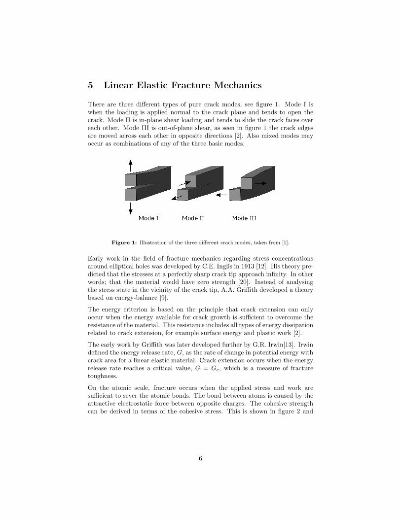
There are three different types of pure crack modes, see figure 1. Mode I iswhen the loading is applied normal to the crack plane and tends to open thecrack. Mode II is in-plane shear loading and tends to slide the crack faces overeach other. Mode III is out-of-plane shear, as seen in figure 1 the crack edgesare moved across each other in opposite directions [2]. Also mixed modes mayoccur as combinations of any of the three basic modes.

Figure 1: Illustration of the three different crack modes, taken from [1].

Early work in the field of fracture mechanics regarding stress concentrationsaround elliptical holes was developed by C.E. Inglis in 1913 [12]. His theory pre-dicted that the stresses at a perfectly sharp crack tip approach infinity. In otherwords; that the material would have zero strength [20]. Instead of analysingthe stress state in the vicinity of the crack tip, A.A. Griffith developed a theorybased on energy-balance [9].

The energy criterion is based on the principle that crack extension can onlyoccur when the energy available for crack growth is sufficient to overcome theresistance of the material. This resistance includes all types of energy dissipationrelated to crack extension, for example surface energy and plastic work [2].

The early work by Griffith was later developed further by G.R. Irwin[13]. Irwindefined the energy release rate, G, as the rate of change in potential energy withcrack area for a linear elastic material. Crack extension occurs when the energyrelease rate reaches a critical value, G = Gc, which is a measure of fracturetoughness.

On the atomic scale, fracture occurs when the applied stress and work aresufficient to sever the atomic bonds. The bond between atoms is caused by theattractive electrostatic force between opposite charges. The cohesive strengthcan be derived in terms of the cohesive stress. This is shown in figure 2 and

6

provides the theoretical strength as

σc ≈E

π(5.1)

Experiments have, however, shown that the actual fracture strength is severalorders of magnitude lower than the theoretical value. This discrepancy is relatedto stress concentrations around flaws in the material which magnify the stresseslocally.

Figure 2: Potential energy and force as a function of atomic separation, taken from [2].

Griffith’s energy balance is based on the first law of thermodynamics whichstates that a system that goes from a state of nonequilibrium to a state ofequilibrium will have a net drecrease in energy. The interpretation of the ap-plication on cracks is that a crack can only grow if the fracture process results

7

in constant or decreased total energy [9]. Hence, the critical condition for crackextension can be defined as the point where crack growth occurs under equilib-rium conditions, with zero net change in total energy [2]. The balance equationunder equilibrium conditions for an incremental increase in crack area, dA, cantherefore be expressed as

dE

dA=dΠ

dA+dWs

dA= 0 (5.2)

which is equivalent to

−dΠ

dA=dWs

dA

where E is the total energy, Ws is the work needed to create two new surfacesand Π is the potential energy in the form of strain energy and work done byexternal forces. For an edge crack, two new surfaces are created when a crackis formed. Thus the expression for Ws takes the form

dWs

dA= 2γs (5.3)

where γs is the material specific surface energy.

Griffith first developed his theory while investigating cracks in glass. It has sincebeen shown that his equation is valid for ideally brittle solids. The theory does,however, greatly underestimate the fracture strength of ductile materials suchas metals. A modification to Griffith’s approach was later developed by Irwinand Orowan [20]. The modified version of the energy-balance equation accountsfor plastic flow. In brittle materials cracks form simply by breaking the atomicbonds, and the surface energy represents the total energy of the broken bondsin a unit area. Crack propagation in ductile metals, on the other hand, includea plastic zone in the vicinity of the crack tip. In this plastic region dislocationmotion occurs. The process of plastic flow around the crack tip contributes toadditional energy dissipation. The modified expression takes the form

Wf = γs + γp (5.4)

where γp is the plastic work per unit area of surface created. It has been shownthat fracture in ductile metals under highly plastic conditions involve dissipationmostly due to plastic work, rather than separation. In other words γs is smallcompared to γp as discussed by Siegmund and Brocks, cf. [24].

Irwin later developed an energy criterion for fracture that is, in essence, equiv-alent to Griffiths criterion. The concept is based on the energy release rate, G,

8

defined as a measure of energy available for an increment of crack extension [2]

G = −dΠ

dA(5.5)

Crack extension occurs when the energy release rate reaches a critical value, i.ewhen

G = Gc =dWs

dA= 2Wf (5.6)

Important to note is that these theories are derived under the assumption thatthe material response is strictly linear elastic. This means that inaccurate resultsmay be produced when applying the model on nonlinear problems. The criterionfor this theory to be valid is that the global behavior of the structure must belinear elastic, while plasticity must be confined to small regions around the cracktip [2].

9

6 Cohesive Zone Modeling of Fracture

Failure and fracture is a big part of many fields in engineering. It is thereforeimportant to understand and to be able to do calculations on failure processesand fractures. To analyze these phenomena efficiently in arbitrary geometries,a general numerical method is needed that can describe the initiation and evo-lution of a crack. The method should include and be able to simulate the initialloading, the damage initiation with initial debonding, and the damage evolutionuntil complete separation and failure has occurred. A method used for thesekind of problems is modeling with cohesive zones. Cohesive zone models havebeen proved useful in many different varieties of fracture issues in homogeneoussolids as well as in analyzing interface crack problems.

For this report a cohesive zone model will be used to analyze crack propagation.For the analysis a numerical FE model will be implemented. The cohesivezone is defined as an interface in between the structure faces where the crackadvance will take place. The interface consists of cohesive elements which areset to behave in the same way as a crack would when it propagates. So for acohesive zone model no elements but the cohesive elements are damaged. Thecrack will only propagate where cohesive elements are modeled. This requires apre-defined crack path.

Cohesive zone models are based on theory from Barenblatt and Dugdale [3, 8].Their method for using cohesive zones to represent a crack propagation pathis very similar to Griffith’s theory based on a surface energy that measures theresistance against crack advance.

Barenblatt and Dugdale’s theory on cohesive zones is based on a method tryingto explain how a crack advances. The cohesive zone is formulated to imitatethe behavior ahead of the crack tip. Both Barenblatt and Dugdale divide thecrack surfaces into two separate regions, one part that is stress free and anotherpart which is loaded by cohesive stresses. Dugdale assumed that there is aplastic zone near the crack tip. Within this plastic zone there is a stress actingacross the crack that is equal to the yield strength, σγ . Dugdale examined theyielding of steel sheets and investigated yielding in the sheets at the end ofslits. He obtained a relation between plastic yielding and external applied loadand found that the influence of yielding was approximately represented by along crack extending into the region that had a stress equal to the yield stress.Dugdale’s theory holds for plane stress but the crack opening stresses can begreater than the equivalent stress in a multiaxial stress state.

Barenblatt investigated brittle materials and instead of a constant stress in thecohesive zone he let the stress vary with deformation in the zone ahead of thecrack tip. The stress of the cohesive zones works as a restraining stress thatkeeps the separating surfaces together. It corresponds to atomic or molecularattractions. The restraining stress, the stress in the cohesive zone, can be seenas a function of the separation distance, σ = σ(δ), see figure 3.

10

Figure 3: The cohesive zone ahead of a crack tip, taken from [3].

Figure 4: To the left is Dugdale’s crack model and to the right is Barenblatt’s crack modelshowing the separation of a crack connected by a cohesive interface, taken from [4].

In figure 4 it is seen in each end of a crack the difference between Dugdale’s andBarenblatt’s theories. Looking at the right end we see Barenblatt’s crack modelwhere the cohesive stress varies with the crack tip displacement. To the left wese Dugdale’s crack model where the cohesive zone has a constant stress equalto the yield stress.

When using cohesive elements a constitutive equation describes the behavior ofthe failing cohesive material elements in front of the crack tip. The constitutiverelation for a cohesive interface is such that the traction across the interfacewill vary depending on the separation of the crack. With increasing separation,the traction will reach a maximum, start to decrease and eventually be reducedto zero. When the traction is zero a complete decohesion is allowed. A typicalcohesive stress-displacement diagram is shown in figure 5. The constitutivebehavior of the cohesive elements is described by a traction-separation law. Theparameters that set the properties of the cohesive zone is the cohesive strength(a peak stress required for separation) and a cohesive energy (separation work

11

per unit area) [25, 27]. The traction-separation laws will be discussed in greaterdetail in the next section.

Looking at figure 3, Γ represents the contour tracing an arbitrary path sur-rounding the crack tip, and δt is the separation distance at the crack tip. Toconnect cohesive theory with Griffith’s work we evaluate the J-integral for thecohesive zone as

J =

∫Γ

(Wdy −T∂u

∂xds) (6.1)

Looking at only the cohesive zone, using path independence and shrinking thecontour Γ down to the lower and upper surface of the cohesive zone, this resultsin dy = 0 on Γ. The J-integral then becomes

J = −∫CZ

σ(δ)dδ

dxdx = −

∫CZ

d

dx

{ δ∫0

σ(δ)dδ

}dx =

δt∫0

σ(δ)dδ (6.2)

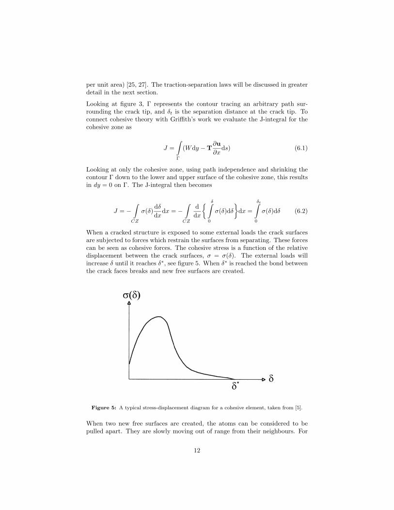
When a cracked structure is exposed to some external loads the crack surfacesare subjected to forces which restrain the surfaces from separating. These forcescan be seen as cohesive forces. The cohesive stress is a function of the relativedisplacement between the crack surfaces, σ = σ(δ). The external loads willincrease δ until it reaches δ∗, see figure 5. When δ∗ is reached the bond betweenthe crack faces breaks and new free surfaces are created.

Figure 5: A typical stress-displacement diagram for a cohesive element, taken from [5].

When two new free surfaces are created, the atoms can be considered to bepulled apart. They are slowly moving out of range from their neighbours. For

12

the process where new free surfaces are created, the cohesive stresses performsome amount of work. The work is written as

W =

δ∗∫0

σ(δ)dδ (6.3)

According to equation (6.2) this relation is equal to the J-integral. To propagatea crack through the distance ∆a, a surface energy is needed which correspondsto

∆Us =

∆a∫0

δ∗∫0

σ(δ)dδdx = ∆a

δ∗∫0

σ(δ)dδ (6.4)

The area under the traction-separation curve is by definition twice the surfaceenergy. Recalling equation (5.3), γs is the surface energy for one new free surfacecreated and for a crack we have two new free surfaces. This gives us

δ∗∫0

σ(δ)dδ = 2γs + γp (6.5)

If the cohesive zone is negligible in size compared to the characteristic lengthsof the structure around the crack it can be concluded that Griffiths theory andthe theory of atomic cohesive forces are identical, cf. equation (5.3).

The information above on cohesive zone models is collected from several authors,see references [1, 8, 15, 17, 19, 21, 29]

6.1 Traction-Separation Laws

The cohesive elements are initially made of a damage-free bulk material whichwill eventually describe the damage and failure of the structure. The damagebehavior is typically described by a traction-separation law, as discussed in theprevious section, also cf. [22].

Depending on the material, one has to choose a suitable traction-separationlaw which correctly describes the fracture behavior of the particular material.The cohesive elements model the initial loading, the damage initiation and thedamage evolution. These three parts can be identified in a curve for the traction-separation law [30].

A basic bilinear traction-separation law, frequently used in calculations, can beseen in figure 6, where the softening after damage initiation is linear. Another

13

model frequently used is the one seen in figure 7, where the softening afterdamage initiation is described by an exponential function. Crack propagationcan be simulated using different parameters that control the advance of the crackfront for cohesive zone models. It can be based on either the local energy releaseor on the separation of the crack surfaces which corresponds to the displacementof the cohesive elements [4].

Figure 6: Illustration of a simple bilinear traction-separation law, taken from [6].

Figure 7: Illustration of exponential damage evolution in a traction-separation law, takenfrom [7].

The bilinear model is uniquely defined by the set of parameters that describesthe top point, (δ0

n,t0n), and the end point, (δtn,0), of the triangle. For both thebilinear and the exponential model the maximum traction sustainable by thecohesive element, tn, is required. This threshold value is important since itgoverns when initiation of damage occurs. The penalty stiffness, K0, is also

14

an important parameter in ensuring realisitic pre-crack conditions. K0 is theslope of the first part of the curve seen in figure 6 and 7. If the penalty stiffnessis insufficient, large displacements will occur in the interface, which alters thebehavior of the structure.

The second part of the curve is related to damage evolution. When assumed tobe linear, it can be defined by either prescribing a failure displacement, δfn, orthe critical energy release rate, Γ0. When the damage evolution is assumed to beexponential the curve can be defined by prescribing a failure displacement, δfn,and a exponential law parameter to define the flexion of the curve. It can alsobe based on the energy, Γ0. When choosing to prescribe failure displacement,the critical energy release rate can be calculated as the area under the curve,and vice versa.

Γ0 =

δ0∫0

T (δ)dδ (6.6)

When modeling fracture in ductile materials, such as steel, the deformationprocess involves the processes of elasticity, plasticity and damage. This meansthat the shape of the traction-separation law cannot easily be determined ex-perimentally, and would have to be assumed [22]. The cohesive model is aphenomenological model. The cohesive model does not model the real physicalfracture process and there is no evidence for which traction-separation law is theright one to use. In the literature there are several different approaches found.

Since there are many different assumptions of the traction-separation law a fewwill be described with reference to the authors. They all build on the samefundamental ideas, but include a few differences.

6.1.1 Tvergaard and Hutchinson

Tvergaard and Hutchinson developed a model for an idealized traction-separationlaw specified on the crack plane to characterize the fracture process in 1992 [27].The relation can be seen in figure 8. The relation is built on an increase of trac-tion in the cohesive element until it reaches the peak traction, σ, at δ1. Thetraction will stay the same for further separation until δ2 is reached. Thendamage evolution is modeled until reaching δc where fracture occurs.

The energy disspated by the cohesive elements at failure is defined by the areaunderneath the curve. For this specific curve, the expression for the work ofseparation per unit area in equation (6.6) takes the following form

Γ0 =

δ1∫0

σdδ =1

2σ[δc + δ2 − δ1] (6.7)

15

To fully specify Tvergaard and Hutchinsons separation law the parametersneeded to describe the fracture process are the work of separation per unitarea, Γ0, and the peak traction, σ. Shape parameters are δ1

δcand δ2

δc[27]. We

also need a set of parameters to describe the continuum behavior of the solid.The elastic-plastic solid is characterized by the following expression

ε =

{σ/E σ ≤ σy

(σy/E)(σ/σy)1N σ ≥ σy

(6.8)

The solid is specified by its Young’s modulus, E, the Poisson’s ratio, ν, theinitial tensile yield stress, σy, and the strain hardening exponent, N .

Figure 8: Graphical illustration of Tvergaard and Hutchinsons traction-separation law, takenfrom [8].

Tvergaard and Hutchinsons suggestion is shown mostly to be suitable for ductilefracture.

6.1.2 Needleman

A cohesive zone model which takes finite geometry changes into account pro-posed by Needleman [16], is used to provide a description of the behavior of voidnucleation. The model is aimed to describe the evolution from initial debondingthrough to complete decohesion which refers to subsequent void growth in a ma-terial. The decohesion occurring can occur either in a brittle or ductile manner.This is dependent on the ratio of a characteristic length to the inclusion radius.The characteristic length is introduced by the dimensions of the surroundingmaterial e.g. dimensions around a crack tip.

16

The characteristic length that is introduced comes from the fact that the modelis to take finite geometry changes into account. The mechanical response ofthe interface is based on both a critical interfacial strength and the work ofseparation per unit area. Based on this, the characteristic length is introduced.

The interfacial traction is only dependent on the displacement difference acrossthe interface. Consider two points A and B, placed on opposite sides of theinterface. The interfacial traction is then seen as dependent on the displacementdifference, ∆uAB , between the points. For each point of the interface Needlemandefined

un = n · ∆uAB , ut = t · ∆uAB , ub = b · ∆uAB (6.9)

and

Tn = n ·T, Tt = t ·T, Tb = b ·T (6.10)

For the equations (6.9) and (6.10), n, t, b form a right-handed coordinate systemwhere un represents the interfacial separation. A positive un corresponds toincreasing separation and a negative un corresponds to decreasing separation.The constitutive relation for the mechanical response of the interface gives adependence of the tractions (Tn, Tt, Tb) on the separations (un, ut, ub). Theresponse can be specified as a potential φ(un, ut, ub), being defined as

φ(un, ut, ub) = −u∫

0

[Tndun + Ttdut + Tbdub] (6.11)

Needleman’s model resembles the other traction-separation laws in the way thatwith increasing separation of the interfaces, the traction reaches a maximumvalue, then start to decrease to eventually vanish. When the interfacial tractionhas vanished complete decohesion occurs. The specific potential function thatis used is the following

φ(un, ut, ub) =

27

4σmaxδ

{1

2

(unδ

)2[1 − 4

3

(unδ

)+

1

2

(unδ

)2]

+1

2α

(utδ

)2[1 − 2

(unδ

)+

(unδ

)2]+

1

2α

(ubδ

)2[1 − 2

(unδ

)+

(unδ

)2]}(6.12)

17

The interface is undergoing a purely normal separation, ut ≡ ub ≡ 0, δ is thecharacteristic length and α specifies the ratio of shear to normal stiffness ofthe interface. By differentiating equation (6.12) we can obtain the tractions,T = ∂φ

∂u .

Tn = −27

4σmax

{(unδ

)[1 − 2

(unδ

)+

(unδ

)2]

+α

(utδ

)2[(unδ

)− 1

]+ α

(ubδ

)2[(unδ

)− 1

]} (6.13)

Tt = −27

4σmax

{α

(ubδ

)[1 − 2

(unδ

)+

(unδ

)2]}(6.14)

Tb = −27

4σmax

{α

(utδ

)[1 − 2

(unδ

)+

(unδ

)2]}(6.15)

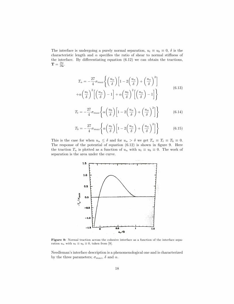
This is the case for when un ≤ δ and for un > δ we get Tn ≡ Tt ≡ Tb ≡ 0.The response of the potential of equation (6.12) is shown in figure 9. Herethe traction Tn is plotted as a function of un with ut ≡ ub ≡ 0. The work ofseparation is the area under the curve.

Figure 9: Normal traction across the cohesive interface as a function of the interface sepa-ration un with ut ≡ ub ≡ 0, taken from [9].

Needleman’s interface description is a phenomenological one and is characterizedby the three parameters; σmax, δ and α.

18

6.1.3 Cornec, Scheider and Schwalbe

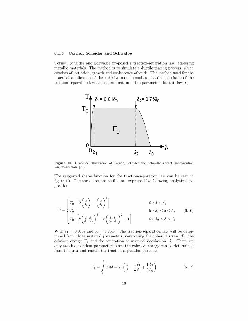
Cornec, Scheider and Schwalbe proposed a traction-separation law, adressingmetallic materials. The method is to simulate a ductile tearing process, whichconsists of initiation, growth and coalescence of voids. The method used for thepractical application of the cohesive model consists of a defined shape of thetraction-separation law and determination of the parameters for this law [6].

Figure 10: Graphical illustration of Cornec, Scheider and Schwalbe’s traction-separationlaw, taken from [10].

The suggested shape function for the traction-separation law can be seen infigure 10. The three sections visible are expressed by following analytical ex-pression

T =

T0 ·

[2

(δδ1

)−(δδ1

)2]for δ < δ1

T0 for δ1 ≤ δ ≤ δ2

T0 ·[2

(δ−δ2δ0−δ2

)3

− 3

(δ−δ2δ0−δ2

)2

+ 1

]for δ2 ≤ δ ≤ δ0

(6.16)

With δ1 = 0.01δ0 and δ2 = 0.75δ0. The traction-separation law will be deter-mined from three material parameters, comprising the cohesive stress, T0, thecohesive energy, Γ0 and the separation at material decohesion, δ0. There areonly two independent parameters since the cohesive energy can be determinedfrom the area underneath the traction-separation curve as

Γ0 =

δc∫0

Tdδ = T0

(1

2− 1

3

δ1δ0

+1

2

δ2δ0

)(6.17)

19

Which in this particular case can be simplified to

Γ0 = 0.87T0δ0 (6.18)

According to Cornec, Scheider and Schwalbe a very simple traction-separationlaw would be chosen just as

Γ0 = T0δ0 (6.19)

But the slopes are chosen to avoid sharp edges. The slope in the beginning helpsout with numerical problems between the cohesive elements and the surroundingcontinuum elements. The slope in after δ2 down to δ0 models the rapid softeningduring void growth and coalescence.

6.1.4 Schwalbe and Cornec

Schwalbe and Cornec [23] suggested a crack growth resistance curve, at fracture,for a material constitutive model that is defined by the parameters σ0, E, ν andn, where n is a strain hardening exponent. They also concluded that the totalwork to fracture can be broken down into three parts; work to separation, ΓS ,plastic energy, ΓP and elastic energy, ΓE . This results in a total energy on theform

J = ΓS + ΓP + ΓE (6.20)

The work of separation and the plastic energy can be allocated to the processzone and the plastic zone, see figure 11. Geometry effects are caused by theplastic energy whilst the separation work is more of a material specific variable.

In the model there are two constants representing the porosity in the material;f0 representing the initial porosity and fc which is the final porosity at frac-ture. These quantities are related to the material’s microstructure. Since themicrostructure of the material is a fundamental part of how the crack will ad-vance these parameters are important and is a fundamental basis of the fracturemodel. Since Schwalbe and Cornec have been looking at a porous model, thisis a brittle fracture process determined by void growth and coalescence.

20

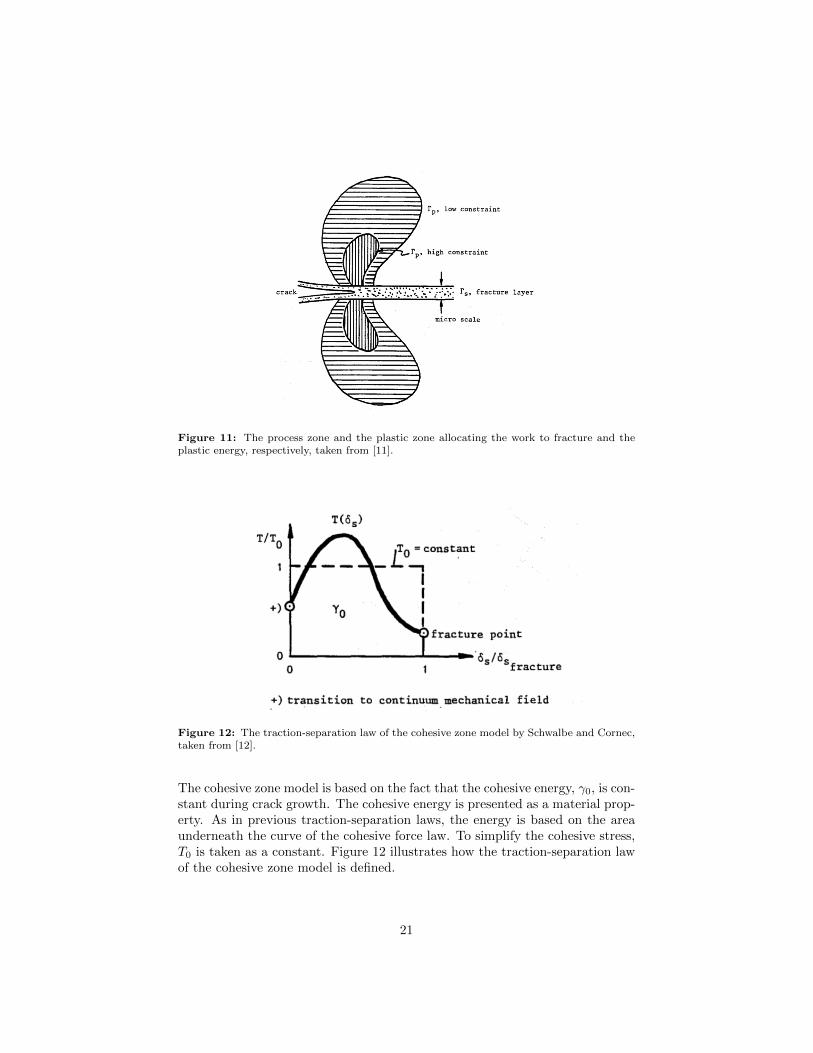
Figure 11: The process zone and the plastic zone allocating the work to fracture and theplastic energy, respectively, taken from [11].

Figure 12: The traction-separation law of the cohesive zone model by Schwalbe and Cornec,taken from [12].

The cohesive zone model is based on the fact that the cohesive energy, γ0, is con-stant during crack growth. The cohesive energy is presented as a material prop-erty. As in previous traction-separation laws, the energy is based on the areaunderneath the curve of the cohesive force law. To simplify the cohesive stress,T0 is taken as a constant. Figure 12 illustrates how the traction-separation lawof the cohesive zone model is defined.

21

The total work equals the cohesive energy and can be expressed as

Ji =

∞∫0

T (δS)dδS ∼= T0 · δS,fracture = γ0 (6.21)

Schwalbe and Cornec used this model to predict crack growth resistance curvesfor various geometries and load versus displacement relationships for structuralparts.

22

7 Cohesive Zone Modeling in Abaqus

Different cohesive zone models can be defined in ABAQUS CAE, which is thepre- and post processor of ABAQUS. In the present study, the cohesive zonemodel is implemented in a double cantilever beam (DCB). A DCB is a goodmodel to be able to investigate the basic behavior of the cohesive elementsand find a traction-separation law that is suitable for predicting crack growth.DCB structures in combination with cohesive zones have been employed in, forexample, [1] and [5]. For the analysis a plane stress condition is implementedfor conditions of small-scale yielding where LEFM applies. Plane stress is usedsince we are looking at a DCB which is small in the thickness direction comparedto the in-plane dimensions.

Arbitrary traction-separation laws are not easily implemented through the CAEinterface. For more general formulations one needs to resort to writing user-defined subroutines.

Since the concept of user-defined subroutine will not be pursued in this reportthe results will be those that are possible to create by just using ABAQUS’sown interface. ABAQUS provides the possibility to define the initial traction-separation stiffness, combined with linear or exponential softening during evo-lution of damage, cf. figure 6 and 7. The damage evolution can be defined bydisplacement or energy.

7.1 Cohesive Zone Element

The cohesive elements are modeled as an own separate part of the model. Thecohesive layer is one element layer thick in between the regions where the crackis to advance. For two-dimensional modeling, the four-node cohesive elementCOH2D4 is used. The cohesive element has a linear displacement formulationand the stress in the third direction does not affect the element behavior andthus there is no difference between plane stress and plane strain condition.The separations and stresses in the cohesive elements are calculated in eachincrement at the integration points according to the traction-separation law.When the critical separation energy is reached, the element has failed. Theintegration point which contributes to the stiffness obtains the status ”failed”.Once a integration point has lost its stiffness, it will never obtain another status[6].

To understand the calculations done by ABAQUS it is interesting to know howthe stiffness matrix of a cohesive element is formulated [21]. It can be derivedfrom the principle of virtual work, which for the cohesive stresses is defined by

δΠi =

∫t · δ[u]dA (7.1)

23

Where the separation is denoted as [u] and t is the vector of the cohesive stressesrelated to the separations.

The coordinates and separations are written, using a FE approximation. Thedisplacements [u] are replaced by

u = Vu · ue (7.2)

Where Vu is a matrix with the shapefunctions and ue is the displacement foreach node. Vu is defined as

Vij =

(f1 0 f2 0 ... fn 00 f1 0 f2 ... 0 fn

)(7.3)

Using equation (7.2) and inserting it into equation (7.1) leads to

δΠi = δ[ue] ·∫

VTu · tdA (7.4)

The cohesive stresses t in equation (7.1) are nonlinear functions of the displace-ment. This makes it impossible to extract the nodal displacement from theintegral, and a linear system of equations can not be setup. This means wewill need to find a tangential stiffness matrix. The tangential stiffness matrixis the change of the internal forces corresponding to infinitesimal changes indisplacements [14].

To find the tangential stiffness matrix, the integral part of equation (7.4) isdifferentiated. The integral in this equation can be seen as the internal forces.

δΠa = δ[ue]f (7.5)

Where

f =

∫VTu · tdA (7.6)

When differentiating the internal forces the total differential of the traction isused as

dt =∂t

∂[u]· du (7.7)

For du the difference ∆u is used. Looking at the total displacement at thetime t+ ∆t we get ut+∆t = ut + ∆u. The next step is to write the differentialformulation of the integral in equation (7.4) so that we can find the tangential

24

stiffness matrix K. Looking at the differential of only the integral it can bewritten as

∫VTu · dtdA =

∫VTu · ∂t

∂[u]·VudA · ∆[ue] = K · ∆[ue] (7.8)

The integration is evaluated numerically using the Gauss integration algorithm,whereby the tangential stiffness matrix can be written as

K =

∫VTu · ∂t

∂[u]·VudA =

∑i

(VTu · ∂t

∂[u]·Vu

)∣∣∣∣i

ωiJi (7.9)

The weight function for the Gauss integration is ωi, Ji is the Jacobian determi-nant of the cohesive element at the specific Gauss point. The Jacobian can becalcuated from the matrix

J =

(∂x∂ε

∂y∂ε

∂x∂η

∂y∂η

)(7.10)

ABAQUS uses the definition for the tangent stiffness matrix shown in equation(7.9) in the FE-calculations for the cohesive zone. In ABAQUS the cohesivezone is modeled between the two potential crack faces and tied to the upperand lower face by tie-constraints, c.f figure 13 [7].

Figure 13: Illustration of the cohesive elements and how they are modeled, taken from [13].

The softening part of the cohesive law often give rise to convergence issues whenrunning the calculations. The analysis tends to exhibit mesh sensitivity, lack of

25

convergence, computing inefficiency, sensitivity to element aspect ratio and soon. These difficulties need to be adressed when using cohesive zones and it isalso very important to pick the right traction-separation law with the correctparameters [28].

26

8 Numerical Examples

Having summarized the basic theory of a cohesive zone model and traction-separation laws attention is now turned to implementation in ABAQUS. Forthe results a linear damage evolution and an exponential damage evolution willbe compared since these are easily accessible in ABAQUS CAE without using auser-defined subroutine to describe the material behavior of the cohesive zone.

8.1 Double Cantilever Beam Model

The cohesive zone model is implemented on a double cantilever beam, see figure14. The material properties for the beam can be seen in table 8.1. The materialis linear-elastic.

Figure 14: The abaqus model of the DCB with dimensions.

Table 8.1: Material parameters for the DCB, representative for steel.

Youngs modulus, E [N/mm2] Poission’s ratio

205 000 0.3

For the DCB analysis displacement controlled loading is used. The top andbottom left nodes of the DCB are the nodes which are subjected to a verticaldisplacement of 8 mm in opposite directions.

Different mesh densities and element sizes are tested to find a mesh which pro-vides an appropriate result for the beam calculation. If the mesh is too coarsetrue behavior will not be captured and a too fine mesh consumes unnecessarytime on calculations for results that are provided also with a coarser mesh. Toidentify a suitable mesh disctretization, only one half of the DCB geometry isused and the simulation results are checked against the analytical expression,found from elementary beam theory, c.f [26], as

δ =Pl3

3EI(8.1)

27

8.2 Comparison of Traction-Separation Laws

For the traction-separations laws, that are used in the cohesive zone model, tobe compared in a consistent way some parameters have to be held constant. Theconstant parameters are the penalty stiffness, K0, and the maximum traction,tn. Further, it is chosen for the traction-separation laws to depend on the criticalenergy release rate, Γ0, also set as a constant. In table 8.2 the values for theparameters can be seen.

Table 8.2: Parameters for the traction-separation law.

K0 10 000 [N/mm3]tn 100 [N/mm2]Γ0 2 [J/mm2]

When comparing the traction-separation laws for the cohesive zone a force-displacement curve will be analysed. The curve will show how the beam re-sponds when the crack advances. By analysing the curve it is then possibleto see if the choice of traction-separation law will make the crack propagationbehave differently.

The mesh for the DCB is tested to find one that is possible to use for all analysesof the cohesive zone. However, the element size in the cohesive zone is also variedto investigate how the results differ with different mesh densities.

The maximum traction chosen will be used for all analyses except one wheredifferent maximum tractions are investigated to see how the results are affected.

8.3 Implementation Issues

There are two different ways to implement the cohesive behavior in ABAQUS.The first includes modeling the cohesive zone as a surface interaction. The othermethod, which is used in this paper, is based on implementing actual cohesiveelements between the two surfaces along the crack path. The surfaces are thenconnected to the cohesive elements using tie constraints. These constraints tiethe nodes on the slave surface, in this case the surface of the cohesive zone, tothe elements of the master surface, i.e. the adjacent solid material.

When modelling the tie constraints there are different options for the discretiza-tion method. One can choose from either ’surface to surface’ or ’node to surface’discretization. For this application it is important to choose the latter to ensurethat all the nodes on the cohesive zone are properly connected to the ligament.

The characteristics of the traction-separation law have a great influence on theconvergence. If the penalty stiffness is too high, sharp increases in stiffnesswill occur in elements which are suddenly loaded. Another parameter whichhas great influence on the convergence is the fracture energy. The fracture

28

energy determines, in the case of the basic triangular traction-separation law,the decrease in stiffness. As with most non-linearities, numerical issues canarise when the material softens rapidly. Lowering of the fracture energy greatlyreduces the stiffness once damage is initiated and can cause convergence issuesdue to sharp decreases in stiffness.

Trying to implement all the traction-separation laws described in this reportwas very difficult. The possibility of completely defining your own traction-separation law is not accessible unless using a user-defined subroutine to definethe cohesive behavior. In ABAQUS CAE it was possible to define the linearand exponential damage evolution and compare these two. For other traction-separation laws as for example Tvergaard and Hutchinson’s, it is recommendedto use a user subroutine to define the cohesive zone behavior.

29

9 Results

In this section the results from ABAQUS are presented. Running the DCBcalculation with different traction-separation laws for the cohesive zone, a de-formation of the beam similiar to the on seen in figure 15 should be obtained.The cohesive elements in figure 15 are seen as just black, this is because the el-ements are too small to distinguish. The magnified cut-out gives a closer view,see figure 16.

Figure 15: The deformation of the DCB after displacement controlled loading. Seen is alsothe deformed cohesive elements modeled inbetween the top and bottom cantilever beams.

The force-deflection curves are represented by values from the top node in theDCB which was subjected to a prescribed displacement. This node representsthe behavior of the beam structure. The graphical illustrations of the traction-separation laws are constructed of values from a node in a cohesive elementwhich is known to have collapsed.

Running the simulation in ABAQUS, a value for the damage variable can beretrieved, varying between zero and one. This variable is a good way to seewhen and if a cohesive element has failed. In figure 17 the red elements indicatea failed element with a damage variable equal to one.

30

Figure 16: A magnified cut out of the DCB when deformed to get a better view of thecohesive elements. The cohesive elements are represented by the blue elements inbetween thebeam parts.

Figure 17: The damage of the cohesive elements with red indicating failure.

9.1 Choice of Mesh for the DCB

The DCB will have an unchanged mesh throughout the analyses. But the choiceof the mesh is determined by analysing the convergence of the result comparedto the element density. Figure 18 is showing the results of testing differentelement densities. The amount of elements are chosen to be 100, 400, 800 and2400. The results obtained with different meshes are compared to the analytical

31

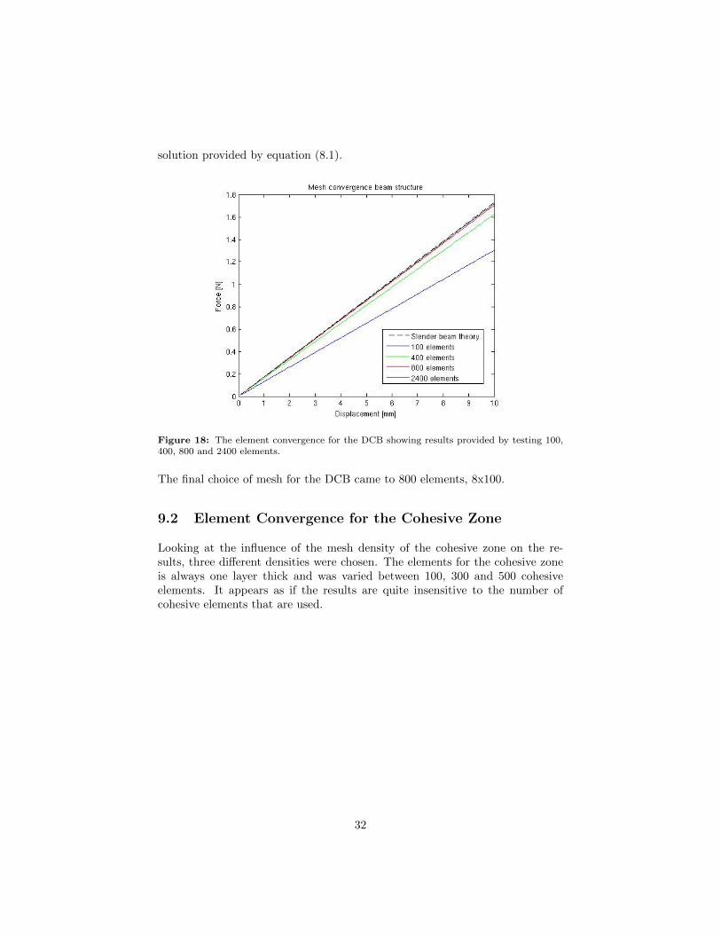
solution provided by equation (8.1).

Figure 18: The element convergence for the DCB showing results provided by testing 100,400, 800 and 2400 elements.

The final choice of mesh for the DCB came to 800 elements, 8x100.

9.2 Element Convergence for the Cohesive Zone

Looking at the influence of the mesh density of the cohesive zone on the re-sults, three different densities were chosen. The elements for the cohesive zoneis always one layer thick and was varied between 100, 300 and 500 cohesiveelements. It appears as if the results are quite insensitive to the number ofcohesive elements that are used.

32

Figure 19: The element convergence for the cohesive zone showing results provided by testing100, 300 and 500 cohesive elements.

9.3 Results for Traction-Separation Laws

Two traction-separation laws are analysed. One which is bilinear and one thatis linear until damage initiation and then has a exponential damage evolution.The results are seen in figure 20, illustrated by a force-deflection curve. Thetraction-displacement curve for the models are shown in figure 21.

Figure 20: Showing the force-displacement curve for the linear and exponential traction-separation law.

33

Figure 21: Showing traction-separation laws for the exponential and linear model.

Looking at figure 20, it appears as both traction-separation models provide verysimilar results, based on the current model set-up.

9.4 Results for Varying Fracture Energy

Seen in figures 22 and 23 are the force-deflection curve and the traction-separationcurves from the simulation where the maximum traction is kept constant andthe fracture energy varies. The fracture energy varies with 2, 3 and 4 J/mm2

Figure 22: Force-deflection curves for the response of the DCB when varying the fractureenergy.

34

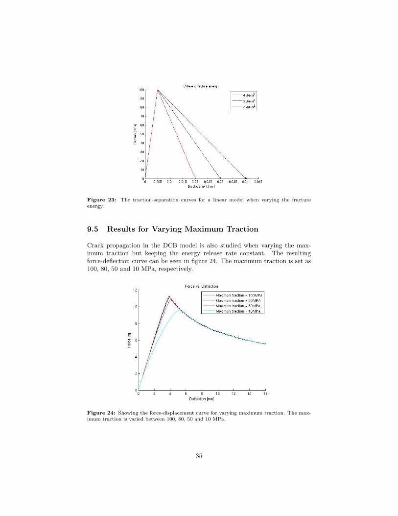
Figure 23: The traction-separation curves for a linear model when varying the fractureenergy.

9.5 Results for Varying Maximum Traction

Crack propagation in the DCB model is also studied when varying the max-imum traction but keeping the energy release rate constant. The resultingforce-deflection curve can be seen in figure 24. The maximum traction is set as100, 80, 50 and 10 MPa, respectively.

Figure 24: Showing the force-displacement curve for varying maximum traction. The max-imum traction is varied between 100, 80, 50 and 10 MPa.

35

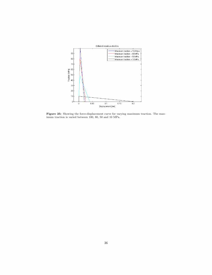
Figure 25: Showing the force-displacement curve for varying maximum traction. The max-imum traction is varied between 100, 80, 50 and 10 MPa.

36

10 Discussion and Conclusions

The double cantilever beam is chosen to have a mesh of 8 elements across theheight and 100 elements along the width. This choice comes from the factthat the amount of elements slowly converges to the result obtained with theelementary beam theory. Looking at figure 18, it is clearly seen that 100 elementsis a too coarse a mesh. The result from ABAQUS with this mesh shows a hugedeviation from the analytical result. Also for 400 elements the difference in theresult is significant. But comparing 800 elements to the analytical result we areclose enough to the correct solution to have an acceptable error. Since thereis very little difference in a solution with 2400 elements and the solution with800 elements, it is concluded that 800 elements gives a satisfying result withoutdegrading the accuracy of the calculations.

The mesh convergence study for the cohesive zone shows that no significantdifference in the results are obtained when using different mesh densities, seefigure 19. The curves for the different counts of cohesive elements coincide.This shows that the number of cohesive elements will not significantly affect theresults. However, the general experience from working with cohesive elementsduring this project is that choosing too few elements can result in instabilityand convergence difficulties. Using a very fine mesh in the cohesive zone can, onthe other hand, lead to very long computation times. The mesh density musttherefore be chosen carefully with these two points in mind.

Using an exponential softening model the calculations was perceived to convergefaster. The linear softening has a good convergence as well but not as good. Thebehavior of the two different models does not show differences in the resultingbehavior of the simulated beam. The crack extends in the same way, which iscontrolled by the fracture energy, and initiates at the same time, due to thechoice of penalty stiffness and maximum traction. Most inequalities are seenafter damage initiation which is when the damage evolution behaves accordingto either of the two different models. The results, however, follow the sameslope and converge to about the same value.

The appearance of the traction-separation laws are seen in figure 21. There isan obvious difference between the shapes of the linear and exponential softeningmodels. The first part of the curve, which is controlled by the penalty stiffnessand the maximum traction, coincides.

The penalty stiffness is mostly set to a very high value since this choice resemblesreality. If the penalty stiffness is too low, the displacement of a cohesive elementwill be quite large before any damage occurs. In reality a crack does not openunless the crack is advancing and damage is evolving. Since a lower penaltystiffness also greatly increases the energy absorbed by the elastic loading partof the curve it reduces the amount of energy available for the damage part ofthe curve for a fix fracture energy. This leads to very steep softening which,in turn, often lead to convergence difficulties. It can be concluded that a high

37

penalty stiffness is needed to ensure realistic pre-crack extension behavior.

The fracture energy, i.e. the area underneath the two curves in figure 21, is thesame for both models. Increasing the fracture energy entails that the failuredisplacement is increased, since the area under the curve must increase. Thedamage initiation will still occur in the same place and at the same time, butthe damage evolution will be a prolonged process. For the force-deflection curvein figure 20, the lowering of the stiffness in the structure is caused by damage. Ahigher fracture energy essentially means that more energy is needed at the cracktip to create new surfaces. Linear elastic fracture mechanics predicts that thefracture energy is proportional to the stress intensity factor squared. Since thestress intensity factor is related to the stress, it is intuitive that a higher load isneeded to advance the crack. This corresponds well with the results presentedin figure 22.

Looking at results from when the maximum traction is varied there is a moresignificant difference in the results from the beam analysis. The maximumtraction varied with a constant energy implies that the failure displacementmust be different. This is seen in figure 25. Since the same amount of energyis needed for the crack to advance, the crack propagation will behave in thesame way. As seen in figure 24, the curves eventually coincides for all choicesof maximum traction. The main thing the maximum traction affects is the pre-crack extension behavior, equal to the softening during the damage evolution.

38

11 Future Work

Writing this report gave us a perspective of how useful cohesive zone modelscan be. Even though it is not yet big in the area of crack propagation in steel ithas huge potential. Most applications today are for brittle materials and veryductile materials, like polymers. The theory on the subject is endless and thereare still much to look into even further. There are a lot of traction-separationmodels for the cohesive zone proposed by different authors and still more tocome. The work on cohesive zones is a long way from being finished.

The review on the cohesive zone theory in this report can be used in manyapplications. Being able to use cohesive zones in FE-programs such as ABAQUSand understanding the approach makes it possible to apply the knowledge onvarious FE-problems involving crack growth.

A proposal on further work with crack advance is to consider Hallberg’s articlefrom 2007 [11]. In this article, a constitutive model for martensite transfor-mation in austenitic stainless steel is derived. In a subsequent article, also byHallberg, from 2011 [10], results are shown from a stationary crack where themartensite transformation at the crack tip is included. Using this constitu-tive model with a cohesive zone model on an advancing crack would make itpossible to investigate how the martensite transformation influences the crackpropagation.

Using a cohesive zone model for this problem one has to consider that thefracture toughness is different for the martensitic and austenitic phases. Thismeans that the material response in the vicinity of the crack tip will change andthe traction separation law will have to account for these changes. An exampleof possible alterations that could be made to the cohesive zone model to accountfor the phase transformation could be by varying fracture energy and maximumtraction to account for changes in fracture toughness and yield stress.

A good idea to look into is also the comparison of the results in this reportagainst further analytical results.

All traction-separation laws decribed in this paper were not implemented inABAQUS. The models presented by Tvergaard and Hutchinson and Scheiderand Cornec proved to be difficult to implement using ABAQUS CAE. In orderto implement these models user-defined subroutines are called for. This was notdone in this project due to lack of time, but it would be of great interest to dothis and compare the results with the ones presented in this paper.

39

12 References

[1] G. Alfano, M. A. Crisfield, Finite Element Interface Models for Delami-naion Analysis of Laminated Composites: Mechanical and ComputationalIssues. 2001

[2] T.L. Andersson, Fracture Mechanics - Fundamentals and Applications.Department of Mechanical Engineering, Texas A&M University. CRCPress, 1991.

[3] G.I. Barenblatt, The Mathematical Theory of Equilibrium Cracks in Brit-tle Fracture. Advances in Applied Mechanics vol. 7, pp 55-129, 1962

[4] J. Chen M. Crisfield, Predicting Progressive Delamination of CompositeMaterial Specimens via Interface Elements. Mechanics of Composite Ma-terials and Structures 6:301-317, 1999

[5] M.A. Crisfield, G.A.O. Davies, H.B. Hellweg, Y. Mi, Progressive Delami-nation Using Interface Elements. Journal of Composite Materials, 1998

[6] A. Cornec, I. Scheider, K-H. Schwalbe, On the Practical Application of theCohesive Model. Institute for Materials Research, GKSS Research CentreGeesthacht, 2003

[7] T. Diehl, Modeling Surface-Bonded Structures with ABAQUS CohesiveElements: Beam-Type Solutions.

[8] D.S. Dugdale, Yielding of Steel Sheets Containing Slits, Engineering De-partment, Univeristy College ov Swansea, 1959

[9] A.A.Griffith, The Phenomena of Rupture and Flow in Solids. 1920

[10] H. Hallberg, L. Bank-Sills, M. Ristinmaa, Crack Tip TransformationZones in Austenitic Stainless Steel. Division of Solid Mechanics, LundUniversity, 2011

[11] H. Hallberg, P. Hakansson, M. Ristinmaa, A Consitutive Model for theFormation of Martensite in Austenitic Steels under Large Strain Plasticity.Division of Solid Mechanics, Lund University, 2007

[12] C.E Inglis, Stresses In a Plate Due to the Presence of Cracks and SharpCorners. Cambridge, 1913

[13] G.R Irwin, Analysis of Stresses and Strains Near the End of a CrackTraversing a Plate. Journal of Applied Mechanics 24, 361–364, 1957

[14] S. Krenk, Non-Linear Modeling and Analysis of Solids and Structures.Cambridge University Press, 2009

[15] N. Moes, T. Belytschko, Extended Finite Element Method for CohesiveCrack Growth. Department of Mechanical Engineering, Northwestern Uni-versity, USA, 2001

40

[16] A. Needleman, A Continuum Model for Void Nucleation by InclusionDebonding. Division of Engineering, Brown University, 1987

[17] A. Needleman, An Analysis of Decohesion Along an Imperfect Interface -1988. International Journal of Fracture vol.42 pp.21-40, 1990

[18] F. Nilsson, Fracture Mechanics - From theory to applications. Royal In-stitute of Technology, 2001

[19] J.R. Rice, A Path Independent Integral and the Approximate Analysis ofStrain Concentration by Notches and Cracks. Journal of Applied Mechan-ics Vol. 35, pp. 379-386, 1968

[20] D. Roylance, Introduction to Fracture Mechanics. 2001

[21] I. Scheider, Cohesive Model for Crack Propagation Analyses of Struc-tures with Elastic-Plastic Material Behavior. GKSS Research CenterGeesthacht, 2001

[22] I. Scheider, W. Brocks, The Effect of the Traction Separation Law on theResults of Cohesive Zone Crack Propagation Analyses, 2003

[23] K-H. Schwalbe, A. Cornec, Modelling Crack Growth Using Local ProcessZones. GKSS Research Centre Geesthacht, Germany, 1994

[24] T. Siegmund, W. Brocks A Numerical Study on the Correlation Betweenthe Work of Separation and the Dissipation Rate in Ductile Fracture. 2000

[25] T. Siegmund, W. Brocks, The Role of Cohesive Strength and SeparationEnergy for Modeling of Ductile Fracture. Fatigue and Fracture Mechanics:30th Volume, 2000, pp. 139-151.

[26] B. Sundstrom and other writers, Handbok och Formelsamling iHallfasthetslara. Institutionen for hallfasthetslara KTH, 1998

[27] V. Tvergaard, J.W. Hutchinson, The Relation Between Crack Growth Re-sistance and Fracture Process Parameters in Elastic-Plastic Solids. 1992

[28] D. Xie, A.M. Waas, Discrete Cohesive Zone Model for Mixed-Mode Frac-ture Using Finite Element Analysis. Department of Aerospace Engineer-ing, The University of Michigan, 2006

[29] A. Yavari, Generalization of Barenblatt’s Cohesive Fracture Theory forFractal Cracks. California Institute of Technology, 2001

[30] Abaqus Analysis, User’s Manual: Volume IV. Dassault Systemes, 2011

41

13 References - Images

[1] Date that collected: 2014-12-09http://upload.wikimedia.org/wikipedia/commons/thumb/e/e7/

Fracture_modes_v2.svg/2000px-Fracture_modes_v2.svg.png

[2] Image from figure 2.1 inT.L. Andersson, Fracture Mechanics - Fundamentals and Applications.Department of Mechanical Engineering, Texas A&M University. CRCPress, 1991.

[3] Image from figure 7a inJ.R. Rice, A Path Independent Integral and the Approximate Analysis ofStrain Concentration by Notches and Cracks. Journal of Applied Mechan-ics Vol. 35, pp. 379-386, 1968

[4] Image from figure 1.1 inI. Scheider, Cohesive Model for Crack Propagation Analyses of Struc-tures with Elastic-Plastic Material Behavior. GKSS Research CenterGeesthacht, 2001

[5] Image from figure 3b inA. Yavari, Generalization of Barenblatt’s Cohesive Fracture Theory forFractal Cracks. California Institute of Technology, 2001

[6] Image from figure 31.5.6-1 inAbaqus Analysis, User’s Manual: Volume IV. Dassault Systemes, 2011

[7] Image from figure 31.5.6-5 inAbaqus Analysis, User’s Manual: Volume IV. Dassault Systemes, 2011

[8] Image from figure 1 inV. Tvergaard, J.W. Hutchinson, The Relation Between Crack Growth Re-sistance and Fracture Process Parameters in Elastic-Plastic Solids. 1992

[9] Image from figure 1 inA. Needleman, A Continuum Model for Void Nucleation by InclusionDebonding. Division of Engineering, Brown University, 1987

[10] Image from figure 2 inA. Cornec, I. Scheider, K-H. Schwalbe, On the Practical Application of theCohesive Model. Institute for Materials REsearch, GKSS Research CentreGeesthacht, 2003

[11] Image from figure 2 inK-H. Schwalbe, A. Cornec, Modelling Crack Growth Using Local ProcessZones. GKSS Research Centre Geesthacht, Germany, 1994

[12] Image from figure 3b inK-H. Schwalbe, A. Cornec, Modelling Crack Growth Using Local ProcessZones. GKSS Research Centre Geesthacht, Germany, 1994

42

[13] Image from figure 31.5.3-2 inAbaqus Analysis, User’s Manual: Volume IV. Dassault Systemes, 2011

43