investigation of membrane potentials in bacterial biofilms
TRANSCRIPT

Investigation of membrane potentials in bacterial biofilms' communication and
stress response
A thesis submitted to The University of Manchester for the degree of
Doctor of Philosophy in the Faculty of Science and Engineering
2020
Johanna A. Blee
Department of Physics and Astronomy

2
Blank page

2
Table of contents
Table of contents 2
List of figures and tables 5
Abstract 1
Declaration 2
Copyright and ownership of intellectual property rights 3
Acknowledgements 5
Publications 6
1 Introduction 7
1.1 Bacterial biofilms 7
1.1.1 Overview 7
1.1.2 The extracellular polymeric substance 9
1.1.3 Biofilm lifecycle 10
1.1.4 Biofilm coordination and regulation 12
1.1.5 Biofilm tolerance and response to stress 13
1.2 P. aeruginosa and B. subtilis 14
1.3 Bacterial ion channels 19
1.4 Membrane potentials 20
1.5 Membrane potentials in biofilms 23
1.6 Outline 24
2 Background and methodology of experimental techniques 26
2.1 Fluorescence microscopy 26
2.1.1 Theory 26
2.1.2 Experimental methodology 30
2.2 Microbiological techniques 33
2.2.1 Background 33
2.2.2 Experimental methodology 36
2.3 Mathematical modelling of excitable systems 40
2.3.1 Theoretical background 40
2.3.2 Modelling methodology 46
3 Spatial propagation of electrical signals in circular biofilms 47
3.1 Overview 47
3.2 Introduction 47
3.3 Materials and methods 52

3
3.3.1 Cell culture and growth 52
3.3.2 Biofilm growth 53
3.3.3 Microscopy 55
3.3.4 Dyes 55
3.3.5 Data analysis 56
3.3.6 Modelling 57
3.4 Results 63
3.4.1 Electrical signalling in circular B. subtilis biofilms (experimental results and
characterisation) 63
3.4.2 Modelling the propagation of electrical signals in circular biofilms 68
3.5 Discussion 79
3.6 Conclusions 82
4 Membrane potentials, oxidative stress and the dispersal response of bacterial
biofilms to 405 nm light treatment 83
4.1 Overview 83
4.2 Introduction 84
4.3 Materials and Methods 85
4.3.1 Cell culture and growth 85
4.3.2 Cell preparation for microscopy 86
4.3.3 ROS scavengers 89
4.3.4 Microscopy 90
4.3.5 Data analysis 92
4.3.6 Mathematical modelling 94
4.4 Results 95
4.4.1 Physical response of P. aeruginosa cells to 405 nm light treatment 95
4.4.2 Membrane potential changes for P. aeruginosa in response to 405 nm light
stress 101
4.4.3 The response of fixed cells 111
4.4.4 Probing the dynamics and timescales of the hyperpolarisation response 112
4.4.5 Response in the presence of scavengers 114
4.4.6 The response of B. subtilis to 405 nm light 116
4.4.7 Hodgkin-Huxley model for the stress response 119
4.5 Discussion 125
4.6 Conclusions 129
5 Measuring c-di-GMP levels and the membrane potential response of Pseudomonas
aeruginosa exposed to oxidative stress 131
5.1 Overview 131
4
5.2 Introduction 131
5.3 Materials and methods 134
5.3.1 Cell culture and growth 134
5.3.2 The c-di-GMP reporter PA01 pCdrA::gfpc and the GFP control strain PA01:gfp 136
5.3.3 Transformation of pCdrA::gfpc into P. aeruginosa PA01 by electroporation 138
5.3.4 Plate reader assay 139
5.3.5 Cell preparation for single cell fluorescence microscopy 140
5.3.6 Microscope set-up 141
5.3.7 Fluorescent dyes and GFPs 141
5.3.8 405 nm light treatment and photobleaching using 488 nm light 141
5.3.9 Irradiance/dose measurements 142
5.3.10 Data analysis 142
5.4 Results 143
5.4.1 Confirming the suitability of P. aeruginosa PAO1 pCdrA::gfpc as a reporter of c-
di-GMP levels 143
5.4.2 Changes in c-di-GMP levels in response to 405 nm light 144
5.4.3 Changes in c-di-GMP levels in response to H202 146
5.4.4 Membrane potential response to H202 149
5.5 Discussion 150
5.6 Conclusions 154
6 Conclusions 156
7 Bibliography 161
Word count: 42, 710

5
1
List of figures and tables
Figure 1.1. Two pictures showing problematic biofilm growth. (a) Biofilm growth in a silicone
catheter, removed from patient after blockage4. (b) Microbial-induced corrosion in a
pipeline5. ........................................................................................................................... 8
Figure 1.2. Schematic diagram showing the five main stages of biofilm growth. Cells are
shown in red and EPS in yellow. (Stage I) Initial cell attachment: planktonic cells reversibly
attach to the surface, often by their poles. (Stage II) Irreversible attachment: cells attach to
the surface and begin to grow and divide colonising the surface. This transition is associated
with a loss of motility and an increase in the production of EPS. (Stage III) Aggregation: cells
continue to grow and divide forming cell clusters and aggregates. (Stage IV) Biofilm
formation: the cell density increases and cells begin to attach to surface cells which are
encased in an EPS. (Stage V) Mature biofilm formation: the biofilm has a complex three-
dimensional structure, with cells embedded in a complex EPS. Following biofilm maturation,
the biofilm disperses and cells return to the planktonic state, facilitating colonisation of new
surfaces. ......................................................................................................................... 10
Figure 1.3. Scanning electron micrograph of a B. subtilis biofilm on a chickpea root38.
Scanning electron micrograph of a P. aeruginosa biofilm on glass wool39. ....................... 15
Figure 1.4. Flowcharts of two biofilm regulation feedback loops. (a) Wsp feedback loop
involved in regulation of P. aeruginosa biofilm growth. (b) Feedback loop showing the
regulation of B. subtilis biofilm growth via Spo0a. ........................................................... 17
Figure 1.5 Illustration showing the distribution of potassium, sodium and chlorine ions
across a typical phospholipid cell membrane in a eukaryotic cell. .................................... 21

6
Figure 2.1. Fluorescent properties of a typical fluorophore. (a) Jablonski diagram showing
the electronic states of a fluorophore and its transitions from one to another energy level.
The thicker lines represent electronic energy levels, while the thinner lines denote the
various vibrational energy states (rotational energy states are ignored). (b) Spectral profile
of a fluorophore showing the Stokes shift observed between the excitation to emission
profiles. ........................................................................................................................... 27
Figure 2.2. Schematic diagram of the custom-built Olympus IX-71 inverted fluorescence
microscope. The laser beams were guided into the microscope by a combination of regular
and dichroic mirrors. The lasers were selectively filtered by a cube that contained a Semrock
Brightline full-multiband laser filter set. Fluorescence was detected using an ORCA-Flash4.0
LT PLUS Digital CMOS camera. ........................................................................................ 32
Figure 2.3. Step-by-step schematic showing the basic process used to culture bacterial cells.
Cells were streaked on to an agar plate, which was then incubated overnight. A single colony
from the plate was then picked from the plate and used to inoculate the culture which, after
further incubation, was used for further cell culture or to grow a biofilm, depending on the
experiment. ..................................................................................................................... 36
Figure 2.4. Schematic of the two different experimental set-ups used to grow biofilms. (a)
CellASIC ONIX microfluidic experimental set-up. (b) Syringe pump flow cell experimental set-
up. .................................................................................................................................. 39
Figure 2.5 Simple model of a cell membrane with a capacitor (𝐶𝑚) in parallel with a resistor.
....................................................................................................................................... 41
Figure 3.1. Proposed mechanism of active propagation of potassium through B. subtilis
biofilms83. The initial trigger for potassium release via Yug0 channel is metabolic stress, due
glutamate limitation. External potassium depolarizes neighbouring cells, limiting glutamate

7
uptake and thus produces further metabolic stress. This cycle results in the active
propagation of potassium through the biofilm. ............................................................... 49
Table 3.I. Recipes and sources for the culture media used in this chapter. ........................ 52
Figure 3.2. Illustrative figure showing how biofilms were grown in the CellASIC ONIX Y04D
plate (not to scale). (a) Schematic of a whole CellASIC ONIX Y04D plate, showing the four
identical, separate chambers, each with 6 inlet wells, a waste outlet well and a cell inlet
well. (b) Cell culture chamber, with six media inlets, waste outlet, cell inlet and six cell traps.
(c) Representative image of a circular B. subtilis biofilm grown overnight in a microfluidic
chamber. Biofilm cells were stained with the membrane potential dye ThT. .................... 54
Figure 3.3. Electrical wavefront from a B. subtilis biofilm. ThT fluorescence observed at 4 µm
from the centre of the biofilm as a function time. Signals from all angles are shown in blue
and the average signal is shown in red. ........................................................................... 57
Figure 3.4. Normalised cell density as a function of radial distance from the biofilm centre
for our experimental centrifugal wavefront data (red), centripetal wavefront data (black)
and agent-based fire-diffuse-fire model (blue). The centripetal biofilm had a larger radius
(~150 m) than the centrifugal biofilm (~90 m). ............................................................ 62
Figure 3.5. Electrical signal propagation through a two-dimensional biofilm. Schematics
show the spread of (a) centrifugal (‘away from the centre’) and (b) centripetal (‘towards the
centre’) electrical wave fronts through a biofilm. (c) The electrical signal given by ThT
fluorescence as a function of time at five different biofilm radii (r = 2 µm, 10 µm, 15 µm, 100
µm and 150 µm) from fluorescence microscopy experiments. .......................................... 63
Figure 3.6. Propagation of centrifugal and centripetal electrical signals through B. subtilis
biofilms. (a) and (b) ThT fluorescence intensity as a function of time and radial distance for

8
a biofilm in which an electrical signal has originated from (a) the biofilm centre (centrifugal)
and (b) the biofilm edge (centripetal). (c) The signals’ fluorescence energy density as a
function of radial distance for the centrifugal wavefront (red) shown in (a) and for the
centripetal wavefront (black) shown in (b), fitted with sigmoids (Equation 3.5). (d) Radial
distance for the maximum intensity as a function of signal mean time for the centrifugal
wavefront (red) shown in (a) and the centripetal wavefront (black) shown in (b), fitted with
power laws (Equation 3.7). .............................................................................................. 66
Figure 3.7. Fire-diffuse-fire model of electrical signal propagation through a B. subtilis
biofilm (Equation 3.8). (a) A plot of 𝑔(𝜈) as a function of 𝜈 for a range of different potassium
decay rates (𝛾). 𝑔(𝜈) is a function which may be used to determine the model’s stability and
thus find constantly propagating solutions to the FDF model (Equation 3.10). (b) The
potassium signal produced by our FDF model of a biofilm (Equation 3.9). (c) The signal
amplitude of the potassium wave shown in (b). (d) The velocity profile (position of the signal
maximum as a function of time) of the signal shown in (b). ............................................. 70
Figure 3.8. Workflow showing the steps executed by our model per time step (Δt). Firstly,
CellSignal was used to update diffusing signalling molecules. Secondly, the cell states were
updated for each cell in the simulation. Finally, CellEngine was used to grow the whole
colony. ............................................................................................................................ 73
Figure 3.9. Snapshots from a Gro simulation of our agent-based fire-diffuse-fire model of a
two-dimensional circular B. subtilis biofilms shown in (a) three-dimensions and (b) two-
dimensions. Snapshots are shown for time since initial firing at the centre of the biofilm T=0,
17, 63 and 120 mins. (c) A magnified image of a potassium wave spreading out from the
centre of the biofilm simulated by our agent-based fire-diffuse-fire model where the
bacterial agents are clearly visible. .................................................................................. 74

9
Figure 3.10. Propagation of (a) centripetal and (b) centrifugal electrical waves produced by
our agent-based fire-diffuse-fire model. The potassium profiles were produced by our model
for a signal triggered at (a) the biofilm centre and (b) the biofilm edge. (c) Fluorescence
energy density, as a function of radial distance, of the centripetal signal (red) and of the
centrifugal signal (black) fitted with sigmoids (Equation 3.5). (d) Radial distance for the
maximum intensity as a function of the signal mean time for the centripetal signal (red)
shown in (a) and the centrifugal signal (black) shown in (b), fitted with power laws (Equation
3.7). For (c) and (d) data was averaged over three separate simulations.......................... 76
Figure 3.11. Kurtosis and skewness of the electrical signal as a function of radial distance.
(a) Kurtosis of our experimental centrifugal wavefront (red) and centripetal wavefront
(black). (b) Skewness of our experimental centrifugal wavefront (red) and centripetal
wavefront (black). (c) Kurtosis of our ABFDF model’s centrifugal wavefront (red) and
centripetal wavefront (black). (d) Skewness of our ABFDF model’s centrifugal wavefront
(red) and centripetal wavefront (black). .......................................................................... 77
Figure 4.1. Schematic showing the ibidi flow cells in which biofilms were grown. (a) Ibidi µ-
slide VI0.4 with six identical channels in which P. aeruginosa biofilms were grown. (b) Ibidi µ-
slide III perfusion flow cell slides with three identical channels in which B. subtilis biofilms
were grown. .................................................................................................................... 87
Figure 4.2. Schematic showing a top and side view of the agarose microscope slide set-up
for fluorescence microscopy. Bacteria were immobilised between the agarose medium and
the microscope coverslip. ................................................................................................ 89
Figure 4.3. Growth curves (OD600) for P. aeruginosa grown in TSB media with and without
10 µM ThT. ...................................................................................................................... 91

10
Figure 4.4. Representative images that depict P. aeruginosa cells stained with ThT at the
five stages of biofilm growth. (a) – (e) show representative cells at Stage I through to Stage
V. .................................................................................................................................... 94
Figure 4.5. Phase contrast images depict the transformational change seen in P. aeruginosa
cells at Stage III of biofilm growth before and after a dose of 1.8 J/ cm2 of 405 nm light. . 96
Figure 4.6. Dispersal response of Stage I P. aeruginosa cells to treatment by 0.1 J/cm2 of 405
nm and 488 nm light. (a) Representative brightfield images show the number of cells before
and after treatment. (b) Graph showing the number of cells before and after treatment. 97
Figure 4.7. (a) Biofilm residence probability as a function of time (or equivalently dose) of P.
aeruginosa biofilms, exposed to 120 ± 4 µW/cm2 405 nm light, for the five stages of biofilm
growth. Corresponding fits of the Kaplan-Meier estimator (𝑆(𝑡), equation (4.3)) shown as
pink dashed lines. (b) The hazard functions ℎ(𝑡) obtained from the Kaplan-Meier functions
(𝑆(𝑡)) shown in (a) at Stage I, II and IV of P. aeruginosa biofilm growth with corresponding
fits shown in red. (c) The cumulative hazard functions 𝐻(𝑡) obtained from the Kaplan-Meier
functions (𝑆(𝑡)) shown in (c) at Stage I, II and IV of P. aeruginosa biofilm growth with
corresponding fits shown in red. (d) The ratio between hazard constants 𝑎𝑡 and 𝑏𝑡 (equation
(4.9)) from hazard functions shown in (b) and (c) at Stages I and Stages II and IV of P.
aeruginosa biofilm growth i.e. growth phases with a significant dispersal of bacteria.
Averages were taken from at least 20 cells in the field of view. ........................................ 99
Figure 4.8. Average ThT fluorescence of Stage II P. aeruginosa cells irradiated with 120 ± 4
µW/cm2 405 nm light as a function of time (or equivalently dose).................................. 102
Figure 4.9. Average ThT intensity of Stage I P. aeruginosa cells as a function of time (or
equivalently dose) observed in response to 405 nm light and 488 nm light, at a constant
irradiance of 480 ± 6 µW/cm2. ....................................................................................... 103

11
Figure 4.10. Average DiSC3(5) intensity of Stage I (a) P. aeruginosa and (b) B. subtilis cells as
a function of time (or equivalently dose) observed in response to 200 ± 4 µW/cm2 405 nm
light (black) and in response to no treatment (red). ....................................................... 104
Figure 4.11. (a) Average cell ThT intensity as a function of time (or equivalently dose)
observed in response to 405 nm light at different stages of P. aeruginosa biofilm growth, in
the same media, at a constant irradiance of 120 ± 4 µW/cm2 with corresponding sigmoidal
fits to equation (4.11). (b) Average ThT fluorescence of mature P. aeruginosa biofilm cells as
a function of time (or equivalently dose) in response to 405 nm light. Data was collected for
a much longer time than that shown in (a) i.e. 900 mins compared to 1500 seconds. .... 108
Figure 4.12. Boltzmann sigmoidal fit parameters (half-maximal dose (D0) and slope constant
𝑥 as given by equation (4.11)) which define the average hyperpolarisation of P. aeruginosa
cells at the five stages of biofilm growth in response to 405 nm light at 120 ± 4 µW/cm2 of
405 nm light. ................................................................................................................. 109
Figure 4.13. (a) Individual cell ThT intensity as a function of time (or equivalently dose),
observed at Stage I of P. aeruginosa biofilm growth, in response to 120 ± 4 µW/cm2 405 nm
light. (b) Leaving time of individual cells from (a) as a function of half-maximal time, with
corresponding linear fit shown in red. (c) The average difference in the leaving time of cells
as a function of cell separation. (d) The average difference in the half-maximal time of cells
as a function of cell separation. ..................................................................................... 110
Figure 4.14. Average ThT fluorescence of trapped P. aeruginosa cells as a function of time
(or equivalently dose) in response to 405 nm light at a constant irradiance of 120 ± 4
µW/cm2. ....................................................................................................................... 112
Figure 4.15. Average ThT fluorescence of trapped P. aeruginosa cells as a function of dose
in response to 405 nm light at an irradiance of 120 ± 4 µW/cm2. The three different curves

12
represent the laser on constantly (black), the laser switched off for 1 min after 15 sec of
illumination (blue) followed by continuous irradiation, and the laser switched off for 1 min
after 1 min on illumination (red) followed by continuous irradiation. ............................. 113
Figure 4.16. Average ThT fluorescence of trapped P. aeruginosa cells as a function of (a)
time and (b) dose in response to 405 nm light at an irradiance of 120 ± 4 µW/cm2. The black
curves represent the laser being on constantly and the red curves represent the response
observed when the laser is turned on once every 0.1 min for 10 ms. .............................. 114
Figure 4.17. (a) Average cell ThT intensity as a function of time (or equivalently dose) of
Stage I P. aeruginosa cells with and without added scavengers (100 mM sodium pyruvate
and 200 U/ml catalase) exposed to 405 nm light at a constant irradiance of 120 ± 4 µW/cm2
with corresponding sigmoidal fits to equation (4.11) shown in blue. (b) Residence probability
(probability of surface cells remaining) of Stage I P. aeruginosa cells following 700 secs
(equivalent to 85 mJ/cm2) of 405 nm light treatment with and without added scavengers
(100 mM sodium pyruvate and 200 U/ml catalase). Errors bars show the standard error.
..................................................................................................................................... 115
Figure 4.18. Biofilm residence probability as a function of time (or equivalently dose) for a
B. subtilis biofilm exposed to 120 ± 4 µW/cm2 of 405 nm light, the Kaplan-Meier estimate
(equation (4.3)) is shown in red, with an inset of the corresponding cumulative hazard
function (equation (4.8)). Averages were taken from at least 20 cells in the field of view.
..................................................................................................................................... 117
Figure 4.19. Average ThT intensity of Stage II B. subtilis cells as a function of time (or
equivalently dose) in response to 120 ± 4 µW/cm2 of 405 nm light. ................................ 118
Figure 4.20. Average cell ThT intensity as a function of time (or equivalently dose) of Stage
I B. subtilis cells with and without added scavengers (100 mM sodium pyruvate and 200

13
U/ml catalase) exposed to 405 nm light at a constant irradiance of 120 ± 4 µW/cm2 with
corresponding sigmoidal fits to equation (4.11) shown in blue. ...................................... 119
Figure 4.21. ThT fluorescence as a function of (a) time and (b) dose in response to 405 nm
light at an irradiance of 120 ± 4 µW/cm2 produced by our Hodgkin-Huxley style model. The
black curves represent the laser being on constantly and the red curves represent the
response observed when the laser is turned on for 10 ms once every 0.1 min. ............... 122
Figure 4.22. (a) Three-dimensional hyperpolarisation curve shows the membrane potential
response to 405 nm light of biofilm cells predicted by our model for a range of input
irradiances (85 µW/cm2 - 575 µW/cm2) as a function of time. (b) ThT fluorescence as a
function of dose in response to 405 nm light at an irradiance of 85 µW/cm2 (black), 185
µW/cm2 (green), 285 µW/cm2 (red) and 385 µW/cm2 (blue) produced by our model. (c) ThT
fluorescence as a function of dose produced by our model in response to 405 nm light at an
irradiance of 120 µW/cm2 which is switched on and off. The black curve represents the dose
response simulated when the laser is on constantly, the blue curve represents the response
observed when the laser is switched on for 45 sec then off for 1 min then back on, and the
red curve represents the response observed when the laser is switch on for 1 min then off
for 1 min then back on. (d), (e) and (f) Hyperpolarisation curves show the membrane
potential with time (or equivalently dose) in response to 120 µW/cm2 of 405 nm light
predicted by our Hodgkin-Huxley style model with corresponding sigmoidal fits to equation
(4.11). (d) Shows simulations of the five stages of biofilm growth based on the assumption
that the rate of ROS production and decay were dependent on the metabolic state of cells
and the stage of biofilm growth. (e) and (f) show simulations of our original and adapted
model in the presence (black) and absence (red) of ROS scavengers, based on the
assumption that the addition of scavengers leads to an increase in the decay rate of ROS.
..................................................................................................................................... 123

14
Figure 5.1. Physiological functions of the intracellular secondary messenger c-di-GMP. C-di-
GMP is synthesised from 2 GTPs via diguanylate cyclases and is degraded into pGpG/GMP
via phosphodiesterases. Extracellular signals control the activity of these proteins and
therefore ultimately regulate the levels of intracellular c-di-GMP. Low levels of c-di-GMP are
associated with the promotion of planktonic behaviour (e.g. motility and acute virulence),
whereas high levels of c-di-GMP are associated with biofilm growth. ............................ 132
Table 5.I. Descriptions and details for the bacterial strains used in this chapter. ............ 135
Table 5.II. Recipes and sources for the culture media used in this chapter. ..................... 135
Figure 5.2. Sequence map of pCdrA::gfpc. (a) Addgene full sequence map for pCdrA::gfpc
created with SnapGene. Shown on the map are: unique 6+ cutters, primers, features and
translations. (b) Schematic showing the horizontal cassette map for pCdrA::gfpc showing
the cdrA promoter fused with the artificial optimized ribosomal binding site (RBSII). The
transcriptional fusion is followed by two transcriptional terminators (T0 and T1). ......... 137
Figure 5.3. Treatment of P. aeruginosa PAO1 pCdrA::gfpc with SNP at concentration of 0
µM, 62.5 µM and 125 µM. (a) Growth measurements given by the OD450. (b) Fluorescence
GFP measurements. ...................................................................................................... 144
Figure 5.4. Treatment of P. aeruginosa PAO1 pCdrA::gfpc and P. aeruginosa PAO1::gfp with
405 nm light. (a) Normalised GFP fluorescence per cell before, following and an hour after
treatment of cells with 3.6 mJ/cm2 of 405 nm light. (b) Photobleaching curves for P.
aeruginosa PAO1 pCdrA::gfpc exposed to 488 nm light at an irradiance of 120 ± 2 µW/cm2
(black) before and (red) after treatment with 3.6 mJ/cm2 of 405 nm light, with exponential
fits given by Equation 5.3. ............................................................................................. 146

15
Figure 5.5. Treatment of P. aeruginosa with 1 mM H202. (a) Ratios of the average GFP
fluorescence to OD600 as a function of time since inoculation for: P. aeruginosa PAO1
pCdrA::gfpc (▲), P. aeruginosa PAO1::gfp (■) and P. aeruginosa PAO1 (●), without H202
(black) and with 1 mM H202 (red). (b) Growth curves of: P. aeruginosa PAO1 pCdrA::gfpc
(▲), P. aeruginosa PAO1::gfp (■) and P. aeruginosa PAO1 (●), without H202 (black) and with
1 mM H202 (red). (c) Ratio of average GFP fluorescence to OD600 , at mid-exponential growth
phase (OD600 ≈ 0.5), without H202 (blue) and with 1 mM H202 (green) for: P. aeruginosa PAO1
pCdrA::gfpc (▲), P. aeruginosa PAO1::gfp (■) and P. aeruginosa PAO1 (●). The presented
errors are standard errors. ............................................................................................ 147
Figure 5.6. Treatment of P. aeruginosa PA01 pCdrA::gfpc and P. aeruginosa PA01::gfp with
H202. (a) Average cell GFP fluorescence of P. aeruginosa PA01 pCdrA::gfpc and P. aeruginosa
PA01::gfp, for a range of H202 concentrations (1 µM, 10 µM, 1 mM and 10 mM), normalised
to the average cell GFP fluorescence without H202. (b) The normalised average cell decay
time constant of photobleaching by 120 ± 2 µW/cm2 488 nm light (Equation 5.3) as a
function of H202 concentration. The inset shows the decrease in cell fluorescence due to
addition of 10 mM H202 in fluorescence microscopy images. The presented errors are
standard errors. ............................................................................................................ 149
Figure 5.7. Membrane potential response of P. aeruginosa treated with H202. (a) Change in
average ThT fluorescence per cell caused by addition of 10 mM H202. (b) Average normalised
ThT (membrane potential) dose response without H202 (black) and with 10 mM H202 (red) in
response to 120 µW/cm2 405 nm light. The presented errors are standard errors. ......... 150
1
Abstract
Bacterial biofilms pose a large threat to health. To understand this resilient and
coordinated form of bacterial growth in more detail the bacterial cells’ membrane
potentials were studied. In circular Bacillus subtilis biofilms, in addition to previously
described electrophysiological waves, which travelled from the centre of the biofilm out to
the edge (centrifugal), waves which travelled from the edge of the biofilms towards the
centre (centripetal) were also observed. New data analysis techniques and an agent-based
fire-diffuse-fire model were used to show that the spatial heterogeneity in bacterial cell
placements and curvature affected the propagation of wavefronts through the biofilm.
The membrane potentials and physical responses of Pseudomonas
aeruginosa and B. subtilis biofilms to 405 nm light were also investigated. It was found that
all cells exhibited membrane potential hyperpolarisations in response to 405 nm light. The
dynamics of these membrane potential changes depended on the stage of biofilm growth.
At the early stages of biofilm growth, cells also dispersed in response to 405 nm light. A
Hodgkin-Huxley style model was used to demonstrate that changes observed during biofilm
growth could explain the observed differences in membrane potential dynamics.
The secondary messenger cyclic di-guanosine monophosphate (c-di-GMP) is a
crucial regulator in biofilm growth in P. aeruginosa. Its role in regulating the oxidative stress
response of P. aeruginosa and the connection between c-di-GMP levels and membrane
potential were investigated using a fluorescence-based GFP reporter strain. Oxidative
stress induced changes in GFP and therefore the GFP-based reporter could not be reliably
used to measure the c-di-GMP levels at high levels of oxidative stress. At low levels of
oxidative stress, the reporter strain was used to show that oxidative stress induced an
increase in the levels of c-di-GMP. This indicates that P. aeruginosa does regulate oxidative
stress via this intracellular messenger and provides a mechanism that drives the dispersal
response of P. aeruginosa to 405 nm light.
Overall, it was shown that bacteria regulate their membrane potentials in response
to a range of different stresses. The data analysis and modelling techniques developed in
this thesis can be used to further study this emerging field of bacterial electrophysiology.

2
Declaration
No portion of the work referred to in the thesis has been submitted in support of
an application for another degree or qualification of this or any other university or other
institute of learning.

3
Copyright and ownership of intellectual property rights
i. The author of this thesis (including any appendices and/or schedules to this
thesis) owns certain copyright or related rights in it (the “Copyright”) and s/he
has given The University of Manchester certain rights to use such Copyright,
including for administrative purposes.
ii. Copies of this thesis, either in full or in extracts and whether in hard or
electronic copy, may be made only in accordance with the Copyright, Designs
and Patents Act 1988 (as amended) and regulations issued under it or, where
appropriate, in accordance with licensing agreements which the University has
from time to time. This page must form part of any such copies made.
iii. The ownership of certain Copyright, patents, designs, trademarks and other
intellectual property (the “Intellectual Property”) and any reproductions of
copyright works in the thesis, for example graphs and tables (“Reproductions”),
which may be described in this thesis, may not be owned by the author and
may be owned by third parties. Such Intellectual Property and Reproductions
cannot and must not be made available for use without the prior written
permission of the owner(s) of the relevant Intellectual Property and/or
Reproductions.
iv. Further information on the conditions under which disclosure, publication and
commercialisation of this thesis, the Copyright and any Intellectual Property
and/or Reproductions described in it may take place is available in the
University IP Policy (see

4
http://documents.manchester.ac.uk/DocuInfo.aspx?DocID=2442 0), in any
relevant Thesis restriction declarations deposited in the University Library, The
University Library’s regulations (see
http://www.library.manchester.ac.uk/about/regulations/) and in The
University’s policy on Presentation of Theses.

5
Acknowledgements
I would like to acknowledge the Engineering and Physical Sciences Research Council
for funding this PhD and making it possible.
I would like to extend my deepest thanks to both my Supervisors, Thomas Waigh
and Ian Roberts, for the time, guidance and wisdom they have provided me with during this
PhD.
I am extremely grateful to Marie Goldrick for sharing her seemingly infinite
microbiological knowledge. I would like to thank all my PhD friends who have given me the
knowledge, coffee, cake and banter to motivate me to the end of this PhD. I would
especially like to thank Hannah Perkins; you really were a large part of making this PhD
enjoyable.
I would finally like to thank my family. I would specifically like to thank my parents,
not just for their continual support and guidance, but for the curiosity and resilience they
instilled in me. Jamie I would like to thank you for, as always, keeping me grounded and
giving me perspective.

6
Publications
Blee, J. A., Roberts, I. S. & Waigh, T. A. Spatial propagation of electrical signals in circular
biofilms: A combined experimental and agent-based fire-diffuse-fire study. Phys. Rev. E 100,
52401 (2019).1
Blee, J. A., Roberts, I. S. & Waigh, T. A. Membrane potentials, oxidative stress and the
dispersal response of bacterial biofilms to 405 nm light. In press. Phys. Biol. 17, 036001
(2020).2

7
CHAPTER
ONE
1 Introduction
An overview will be given of the current understanding of bacterial biofilms with an
emphasis on the importance of regulation, communication and membrane potentials.
Having provided a contextual overview of the project the final section of this chapter will
be used to outline the thesis content.
1.1 Bacterial biofilms
1.1.1 Overview
Bacterial biofilms are communities of bacteria encased in a self-produced
extracellular polymeric substance (EPS). Bacterial biofilms are coordinated multicellular
communities3–5. This prevalent form of growth supports bacterial survival in a wide range
of settings, from the human body to oil pipelines, resulting in a whole host of problems
which are difficult to tackle (Figure 1.1).

8
Figure 1.1. Two pictures showing problematic biofilm growth. (a) Biofilm growth in a silicone
catheter, removed from patient after blockage6. (b) Microbial-induced corrosion in a
pipeline7.
The National Institute of Health estimates that approximately 65 % of all microbial
infections and 80 % of chronic infections are associated with biofilms8. Bacterial biofilms
require antibiotics and biocides at levels 500 to 5000 times higher than planktonic cells9.
This has led to a critical need for new techniques to tackle biofilm growth. Biofilms are also
costly to industry through processes such as biofouling10, adding an extra economic
motivation for combating this form of growth.
Not all biofilms are harmful and they play important, positive roles in the stability
of ecological systems. They also have beneficial applications11, for example, in the
production of industrial chemicals and in treating wastewater. In addition to current
applications, it is hoped they may have further uses, e.g. in the production of biopower12.
The devastating effects of biofilms, paired with the important applications, provide
strong motivation to study this mode of growth. This has been reflected in the large
increase in the study of biofilms in recent decades. It is hoped that a greater understanding
may enable the development of new strategies with which to combat destructive biofilms,
as well as allowing useful biofilms to be harnessed.

9
1.1.2 The extracellular polymeric substance
Central to biofilm growth is the biofilm’s self-produced EPS. Strains of bacteria that
are incapable of producing an EPS (and consequently a biofilm), form homogenous
colonies13. In comparison, bacterial biofilms usually form complex, mushroom-like
structures; with channels which distribute nutrients and remove waste14.
The EPS makes up 75-90 % of the biofilm: giving it structure, contributing to its
genetic regulation and controlling the flow of nutrients and toxins through it4,15. By
impairing the penetration of antibiotic agents and toxic substances the EPS acts as a
diffusion barrier protecting the bacteria it contains. Specific extracellular components, such
as enzymes, have also been shown to actively trap and damage penetrating antimicrobial
agents16,17. One method, employed by several species of bacteria to achieve a robust
biofilm structure, is to synthesise protein fibres that form a shell onto which the microbial
cells and other EPS compounds may attach18.
The EPS produced by the majority of bacteria consists primarily of polysaccharides
combined with eDNA (mitochondrial or nuclear DNA that has been released by the bacteria
into the environment), lipids and extracellular proteins. As well as common constituents,
several novel EPS components have emerged, such as the bacterial hydrophobin, BslA,
which forms a water-resistant ‘raincoat’ over the B. subtilis biofilm19. The exact composition
of the EPS depends on the microbial species and the environment e.g. presence of flow.
This in turn affects key properties of the biofilm, from its mechanical stability to its
hydrophobicity.
Many EPS components remain unquantified and the roles of those that have been
quantified often remain elusive. These components define many of the biofilm’s key
properties and behaviours. Therefore, expanding our understanding of the molecular
function of biofilm components is crucial in developing our knowledge of this mode of
growth.

10
1.1.3 Biofilm lifecycle
Figure 1.2. Schematic diagram showing the five main stages of biofilm growth. Cells are
shown in red and EPS in yellow. (Stage I) Initial cell attachment: planktonic cells reversibly
attach to the surface, often by their poles. (Stage II) Irreversible attachment: cells attach to
the surface and begin to grow and divide colonising the surface. This transition is associated
with a loss of motility and an increase in the production of EPS. (Stage III) Aggregation: cells
continue to grow and divide forming cell clusters and aggregates. (Stage IV) Biofilm
formation: the cell density increases and cells begin to attach to surface cells which are
encased in an EPS. (Stage V) Mature biofilm formation: the biofilm has a complex three-
dimensional structure, with cells embedded in a complex EPS. Following biofilm maturation,
the biofilm disperses and cells return to the planktonic state, facilitating colonisation of new
surfaces.
The details of biofilm growth vary depending on the bacteria, as well as the
environment, but the lifecycle can be broadly described using five stages of growth (Figure

11
1.2)11,20,21. The first step involves the reversible attachment of the planktonic and in some
cases motile cells to a surface. Secondly, these cells attach irreversibly to the surface. This
transition is associated with a loss of motility and an increase in the production of EPS. The
initial and long term attachment of a bacterium to a surface is dependent on the ratio of
attractive and repulsive forces22. These forces can vary significantly for different bacteria
and surfaces; e.g. surfaces with varying compositions and topographies. Attachment is
mediated by forces which are dependent on surrounding conditions, such as available
nutrients and the presence of flow. The interaction between a bacterium and a surface may
also be affected by intermediary factors, such as adhesins23. These not only ensure
attachment and adhesion in the presence of shear stress, but also allow surface specificity.
Some of the forces involved in bacterial and biofilm adhesion remain elusive.
Following attachment the bacterial cells grow and divide to form cell clusters and
aggregates. Additional cells attach to these surface cells. The biofilm continues to grow until
a mature biofilm, with a complex three-dimensional structure emerges. By this stage, the
cells in the biofilm are embedded in a complex EPS. Following biofilm maturation, the
biofilm disperses and cells return to the planktonic state, facilitating colonisation of new
surfaces. Dispersal, which plays a significant role in the spread of bacteria to new
environments, is the least well understood part of the biofilm lifecycle. Dispersion is
triggered and controlled by environmental cues and inter/intracellular signals. To date no
ubiquitous mechanisms of dispersal have been observed and so they remain difficult to
characterise24. In summary, the growth of a biofilm is controlled by a host of physical,
chemical and biological mechanisms, which ultimately determine the structure and
behaviour of the resulting biofilm.

12
1.1.4 Biofilm coordination and regulation
The entire process of biofilm growth, from initial attachment to dispersal, is tightly
regulated21. Biofilm growth relies on the coordination of behaviour between its constituent
bacteria; this is achieved via a complex network of signalling molecules and genetic cues25.
Environmental triggers and secreted quorum sensing molecules both play roles in
regulating the genetic transition of cells from the planktonic to the sessile state and back
again. This is then reinforced by positive feedback loops in which genetic changes cause
cells to produce further influencing factors, such as signalling molecules and enzymes.
One method by which bacteria are known to regulate their cooperative behaviour
is quorum sensing, where communication is achieved via signalling molecules. Quorum
sensing coordinates behaviour based on the local density of the bacterial population.
During this process signalling molecules bind to a receptor on the bacteria, triggering the
transcription of specific genes. A lot of research has focused around identifying different
signalling molecules and the pathways that lead from their production to the alteration of
gene expression. Quorum sensing was initially discovered as a method for regulating
bioluminescence, but has since been identified in association with a range of behaviours.
Some signalling molecules are specific to one microbial species, while others can regulate
communication between a diverse range of species. Several examples of eukaryotes
developing mechanisms to counteract quorum sensing have also been reported26. For
example, one study found that epithelial cells quench the activity of the P. aeruginosa
3OC12-homoserine lactone autoinducer27. It is hoped that methods employed by hosts to
interrupt microbial communication may be mimicked and adapted to target biofilms.
Variations between different biofilms do not only depend on the microbial species,
but also on the environmental growth conditions. Universal mechanisms, for example of
communication, offer particularly attractive targets from which to develop treatments, as

13
they may offer a more widespread solution, where only minor adaptations need to be made
depending on the type of biofilm.
1.1.5 Biofilm tolerance and response to stress
The prevalence and increased resistance of biofilm cells to environmental stress
stems from increased adaptation abilities, as well as due to increased protection offered by
the EPS and neighbouring cells. Mature biofilms are built from heterogeneous,
phenotypically distinct sub-populations, each of which fulfil distinct roles28. Individual cells
cooperate and compete within a complex framework, that is often likened to our own
multicultural cities. Specific phenotypes are associated with distinct locations and growth
stages, indicating spatio-temporal regulation28. Different phenotypes are expressed in
response to varying conditions (e.g. pH, O2 and nutrients) across the biofilm as well as
stochastic gene expression.
The heterogeneity of bacteria ensures survival in variable environments in a bet
hedging strategy. One example of specific cells which survive stressful conditions are
persister cells, which are found deep within biofilms29. They have a decreased metabolic
activity and so have a higher antibiotic tolerance as antibiotics predominantly target cell
growth. They also show higher tolerance to oxidative stress, for example, the viability of
stationary phase cultures of B. subtilis is not affected by treatment with 10 mM H2O2,
whereas the viability of exponential phase cells is reduced to approximately 0.01 %30.
Another protective genetic method used by bacteria is horizontal gene transfer. Transfer of
advantageous genes is key to the evolution of bacteria and their resistance to antibiotics.
The efficiency of this process is enhanced within biofilms31.
The resistance of bacteria to environmental stress is strongly dependant on the
mode of growth (planktonic vs biofilm). During planktonic growth individual cell
14
characteristics are crucial, whereas during biofilm growth, the influence of external
protective elements and surrounding cells is often more important. A combination of
different mechanisms are employed by bacteria and by biofilms to ensure survival and
adaptation to environmental stresses. This is demonstrated by the response of cells to
photooxidative stress. Individual characteristics, such as pigmentation, are key for
photoprotection at a range of wavelengths32,33, while external factors and surrounding cells
can influence both photoprotection and the magnitude of the evoked response to
photooxidative stress. Biofilm cells are more resistant to photoinactivation by light over a
range of wavelengths. It is expected that a range of factors contribute to this increased
resistance. Firstly, some biofilm cells enter a dormant metabolic state, which is known to
be associated with decreased ROS production. Higher levels of catalase, which significantly
protect against oxidative stress, have also been detected in biofilm cells34. Finally, biofilm
cells are encased in a complex EPS, which is known to play a major role in protection. Biofilm
matrix components, such as alginate, protect biofilms by shielding them from light35, while
other components, such as cellulose and alginate, also protect against reactive oxygen
species generated under stress36.
1.2 P. aeruginosa and B. subtilis
Two model bacterial species, P. aeruginosa and B. subtilis, were used in this project
(Figure 1.1). P. aeruginosa is a Gram-negative bacterium, which causes difficult to treat,
nosocomial infections, in particular, topical skin infections and chronic lung infections in
cystic fibrosis patients37,38. In addition, P. aeruginosa can cause biofouling on nano-filtration
devices involved in seawater desalination systems39.

15
B. subtilis is a Gram-positive, spore forming bacterium, that is ubiquitous in the
environment20. It has been studied in the laboratory for over a century, leading to the
domestication of commonly used strains, such as 168. These strains show a distinct
attenuation in their ability to form biofilms when compared to wild type strains, such as
NCIB361013. Domestication can introduce mutations which impair the bacteria’s ability to
swarm on surfaces and form robust structures13.
Figure 1.3. Scanning electron micrograph of a B. subtilis biofilm on a chickpea root40.
Scanning electron micrograph of a P. aeruginosa biofilm on glass wool41.
The regulation of biofilm formation is a complex process, which is still not fully
understood. It is affected by a large number of regulatory pathways and feedback loops. By
examining mutations in strains that are incapable of biofilm formation and by introducing
mutations into wild type strains, knowledge may be gained regarding the genetic regulation
of biofilm growth. One of the key bacterial secondary messengers in biofilm regulation is
c-di-GMP. Its role in regulating the transition from the planktonic to the sessile state and
back again (dispersal) has been extensively studied, especially in model organisms such as
P. aeruginosa42–44. C-di-GMP regulates a host of biofilm associated behaviour from flagella
rotation to exopolysaccharide production, surface adhesin expression and antimicrobial
resistance44–46. The versatility and adaptation capabilities of P. aeruginosa are linked with a

16
large array of complex regulatory networks, including a broad range of genes involved in c-
di-GMP production and degradation. Diguanylate cyclases (DCGs) and phosphodiesterases
(PDEs) are responsible for the biosynthesis and the degradation of c-di-GMP, respectively.
The catalytic domains of DGCs carry a GGDEF site and PDEs carry either an EAL or HD-GYP
domain. These domains are often seen in conjunction with a receiver or transmission
domain, indicating modulation of their activity by external/internal stimuli43. In some
proteins, both GGDEF and EAL domains are present, suggesting a dual function as a DGC
and a PDE. For example, in planktonic P. aeruginosa cells, MucR functions as a DGC,
whereas in biofilm cells, it acts as a PDE47. The P. aeruginosa genome encodes a large
number of DGCs and PDEs, which are modulated by a broad range of signals. In turn, these
proteins regulate a wide range of behaviours. An example of one of these proteins which
regulates and is regulated by biofilm growth is the DGC WspR (Figure 1.4(a)). When a
surface is sensed, the Wsp signal transduction complex phosphorylates WspR and triggers
c-di-GMP synthesis48. In turn, WspR phosphorylation triggers subcellular WspR
oligomerization and cluster formation, increasing the DGC activity49. C-di-GMP then binds
to the l-site inhibiting WspR activity50.
B. subtilis biofilm regulation is primarily dependant on the phosphorylation state of
Spo0a, which is controlled by multiple histidine kinases51. This multicomponent
phosphorelay is affected by a range of stimuli, such as osmotic pressure and potassium
leakage. Spo0a-P produces sinl, which controls the ratio of two transcriptional factors sinR
and slrR. SinR directly represses exopolysaccharide production and promotes flagellar
motility; while SlrR activates biofilm genes and represses motility. One example of an
operon involved in and complexly affected by biofilm formation in B. subtilis is mstX-Yug052.
Expression of mstX and the downstream potassium channel Yug0 is required for biofilm
development and overexpression of mstX may induce biofilm formation. Phosphorylation
of Spo0a is achieved through the histidine kinase KinC, which is activated by potassium

17
efflux through Yug0. SinR negatively regulates the mstX-Yug0 operon and so represses it in
the planktonic state (Figure 1.4(b)).
Figure 1.4. Flowcharts of two biofilm regulation feedback loops. (a) Wsp feedback loop
involved in regulation of P. aeruginosa biofilm growth. (b) Feedback loop showing the
regulation of B. subtilis biofilm growth via Spo0a.

18
Once biofilm formation has been initiated the biofilm’s structure and the
composition of its EPS depends on the genetic expression of cells within it, which in turn
depends on the strain and on the environmental conditions53. The EPS of B. subtilis biofilms
grown in sucrose-rich media, e.g. SYM, is distinctly different from the EPS when grown in
reduced media, e.g. MSgg54. The EPS of biofilms grown in sucrose-rich media is dominated
by the polysaccharide levan, while the EPS from biofilms grown in sucrose-poor media also
contains a significant amount of proteins, DNA and polysaccharides. There are also
differences observed between different experimental setups, for example, the presence of
flow can reduce the thickness of the observed biofilm55.
The main component of the B. subtilis EPS is usually an exopolysaccharide with a
large molecular weight, which is generally formed of the monosaccharides; glucose,
galactose or N-acetyl-galactosamine56. These are synthesised by proteins produced by the
15 gene epsA-O operon. There is limited compositional knowledge of this
exopolysaccharide due to large heterogeneity and due to challenges in polysaccharide
sequencing. The second largest constituent of the EPS is generally the primary protein
element TasA. TasA is an amyloid-like protein that forms fibres that bind cells together57.
Deletion of tasA does not affect surface adhered biofilm formation, implying TasA is not
required for submerged biofilms. The formation of these fibres requires a secondary
protein TapA, and in turn, the production of both these proteins requires the peptidase
SiPW58. This peptidase is multifunctional, with an additional role in the adherence of
submerged biofilms to the surface. The biofilm is assembled with assistance from a
hydrophobin protein BsIA which forms a protective ‘coat’ around the biofilm19.
The EPS of P. aeruginosa PAO1 biofilms contains three polysaccharides: alginate,
Psl and Pel polysaccharides. As for B. subtilis, the presence of different P. aeruginosa EPS
components, depends on the environmental conditions, such as the growth media36.
Alginate deletion mutants develop biofilms with a decreased number of viable cells55. It has

19
also been shown that exposure to oxidative stress induces the overproduction of alginate,
which protects the biofilms from oxidative radicals59. Biofilms of alginate or psl defective
mutants fail to form complex biofilm structures, suggesting these polysaccharides are
structurally important55. The Psl polysaccharide is involved in initial attachment and biofilm
formation60. Pel is essential for the formation of a pellicle at the air-liquid interface, as well
as the formation of wrinkled colonies61.
1.3 Bacterial ion channels
Structural studies of bacterial ion channels have formed the basis of our knowledge
of the general structure of ion channels62. This is because bacterial cells are uniquely suited
to genetic manipulation and have short replication times. They are also easily cultured in
the large quantities required for the production of ion channel proteins, used in structural
analysis, via X-ray crystallography or nuclear magnetic resonance63. Genome sequencing of
ion channels from different cell types (e.g. eukaryotic cells) has confirmed evolutionary links
with bacterial ion channels. Specific genetic sequences may be used to diagnose specific
channel types. For example, the K+ filter sequence-TXGY(F)GD, is used to identify potassium
channels64. Different bacterial ion classes have been explored via structural and
electrophysical methods. We shall firstly discuss ion specific channels, followed by a
discussion on mechanosensitive channels.
The three-dimensional structures of ion specific channels have been resolved to
atomic resolution (potassium, sodium, chloride)65–67. This has allowed identification of
channel structures, such as receptors, these have provided an insight into molecular
mechanisms. Computer models have been used to further understand mechanisms
involved in gating and physiological behaviour68.

20
Structural analysis has shown that most cation specific ion channels have a similar
basic structure. They are composed of four sub units which converge to form the gate which
faces into the cytoplasm69. Various gating principles determine the state of the channel: pH,
ligand binding and membrane potential. Activation of a channel depends primarily on
opening of the gating region, but also on the conductivity of the filter. The ion filter is
located near the outer surface of the cell’s membrane and controls the channel’s specificity.
Despite the depth of structural knowledge on bacterial ion channels, little is known
regarding their role. There are exceptions to this: calcium channels have been shown to be
involved in the extreme acid resistance response and several channels have been shown to
be involved in motility and biofilm formation70. However, the primary role of most channels
remains elusive.
In contrast, the role of bacterial mechanosensitive ion channels (the other main
class of ion channel) is well established71. They act as ‘emergency valves’, releasing solutes
in osmotically challenging conditions, as well as acting as sensors of the cell’s turgor
pressure. A range of different mechanosensitive channels have been characterised via
several different techniques72. For example, electrophysical permeation studies, using large
cations and electron parametric resonance spectroscopy combined with cysteine scanning
mutagenesis and site binding labelling revealed several different channels with varying
conductances73.
1.4 Membrane potentials
Cells maintain a potential across their cell membranes when they are in the resting
state. This membrane potential is established via the asymmetric distribution of ions across
the membrane and is controlled by ion channels. Selective ion channels allow specific ions
to travel down the diffusion gradient, resulting in charge separation. This produces an

21
electrical gradient which increases until it matches the chemical gradient and there is
electrochemical equilibrium74. The equilibrium potential for a single ion is the potential at
which that ion would have no net movement across a membrane if it was the only ionic
species present. This is commonly defined as the Nernst potential75 and is given by,
𝑉𝑋 =𝑅𝑇
𝑧𝐹𝑙𝑛[𝑋]0[𝑋]𝑖
, (1.1)
where 𝑉𝑋 is the Nernst potential for given ion 𝑋, 𝑅 is the universal gas constant, 𝑇 is the
temperature in Kelvin, 𝑧 is the valence of the ionic species and 𝐹 is the Faraday constant.
Equation 1.1 is only valid for one ionic species. However, it can generally be
assumed that the main contributions to a eukaryotic cell’s membrane potential at rest
come from potassium, sodium and calcium. The distributions of these ions across a typical
cell membrane in resting state are shown in Figure 1.5.
Figure 1.5 Illustration showing the distribution of potassium, sodium and chlorine ions
across a typical phospholipid cell membrane in a eukaryotic cell.
The Goldman-Hodgkin-Katz equation takes account of the contributions from all
three of these ions and so, in general, can be used to find a good approximation of a cell’s
equilibrium potential,
𝑉𝑒𝑞 =
𝑅𝑇
𝐹ln𝑃𝑁𝑎[𝑁𝑎
+]𝑜𝑢𝑡 +𝑃𝐾[𝐾+]𝑜𝑢𝑡 +𝑃𝐶𝑙[𝐶𝑙
−]𝑜𝑢𝑡𝑃𝑁𝑎[𝑁𝑎
+]𝑖𝑛 +𝑃𝐾[𝐾+]𝑖𝑛 +𝑃𝐶𝑙[𝐶𝑙
−]𝑖𝑛,
(1.2)

22
where 𝑉𝑒𝑞 is the membrane potential, 𝑃𝑖𝑜𝑛 is the permeability for that ion, [𝑖𝑜𝑛]𝑜𝑢𝑡 is the
extracellular concentration of that ion and [𝑖𝑜𝑛]𝑖𝑛 is the intracellular concentration of that
ion.
The difference between a cell’s membrane potential and the resting potential of an
ionic species leads to efflux/influx of ions under resting conditions, this is counteracted by
actively pumping ions down their electrochemical gradients. Therefore, in most cells, the
resting potential of a cell is established due to charge separation, but is maintained by
active transport of ions across the membrane.
A cell’s membrane potential and many of its crucial physiological processes are
fundamentally linked. The membrane potential depends on the distribution of ions across
the cell membrane and in turn the transport of ions across the membrane is dependent on
the membrane potential. Many key functions of a bacterial cell are dependent on its
membrane potential70,76–79:
1. Uptake of nutrients/ions/toxins.
2. Motility.
3. Cell division is dependent on the arrangement of cell division proteins, which is
determined by the membrane potential.
4. Metabolism.
5. Regulatory pathways and transcription factors.
6. Cell growth.
7. Adhesion.
8. Quality control during sporulation.
The proton motive force (PMF) is a form of metabolic energy which drives the
uptake of many compounds and can be applied to synthesise ATP via F0F1-ATPase. In
general, the proton motive force is generated by a negative membrane potential and an

23
alkaline pH gradient across the membrane. Many of a cell’s functions rely either directly or
indirectly on the existence of a proton motive force, without a negative potential driving
this force, the cell cannot survive. Membrane potential indicators are therefore often used
as a measure of cell viability.
A negative resting potential is not the only way cells use the membrane potential.
Environmental changes may directly (e.g. increases in external ion concentration) or
indirectly (e.g. opening of ion channel by stimulus) result in a change in membrane
potential. These variations may, in turn result in further responses/behavioural changes.
For excitable cells, a signal may be triggered to communicate changes to other cells, in a
process known as an action potential. These excitable cells exploit membrane potential
changes brought about via a change in an environmental variable of interest (stimuli) to
send signals.
1.5 Membrane potentials in biofilms
The cell’s membrane potential and many of its vital physiological processes are
inextricably linked. It is therefore unsurprising that cells in a biofilm respond to changes in
membrane potential and synonymously that the biofilm membrane potential depends on
the state of the biofilms’ cells.
The electrical activity of bacteria in a biofilm has been found to depend on its
growth stage as well its environment. One study observed electrical spiking in the
membrane potential of E. coli that was sensitive to physical and chemical fluctuations80.
Another study found that the cellular response to external electrical stimuli was influenced
by the cellular proliferative capacity81.
The behaviour, physiology and growth of biofilms are modified by electrical
potentials. Application of electric fields and currents can enhance the activity of
antimicrobial agents against biofilms, in a process known as the ‘bioelectric effect’9.

24
Evidence now also exists to support the ‘electricidal effect’82, a process by which electrical
currents affect biofilm viability in the absence of antimicrobial agents. These processes have
received a substantial amount of attention owing to their potential application in
electrochemically active materials for use in medical devices83.
Bacteria in a biofilm receive increased protection, resulting in a prevalent and
stable form of microbial life. Central to this mode of growth is the ability of bacteria to
coordinate behaviour and act as a multicellular organism. Despite this, a significant amount
of biofilm regulation remains poorly understood. The similarity between bacterial ion
channels (with unknown roles) and their excitable eukaryotic counterparts (Section 1.3) is
suggestive of an analogous role in electrical signalling. The strong connection between a
cell’s electrical activity and its state provides a mechanism by which electrical signalling may
influence the behaviour of the biofilm cells.
Even though ion specific channels in bacteria are highly amenable to structural
analysis, electrophysical measurements are technically difficult, especially within biofilms.
This has made studying electrical signalling in bacterial biofilms challenging. Using a
multielectrode array, electric spiking was found to correlate with biofilm formation, leading
to the suggestion of electrical signalling as a driver in biofilm sociobiology84. More recently
fluorescent probes were used by Prindle et al. (2015)85 to present the first direct evidence
of electrical signalling between bacterial cells in a biofilm. Further studies have built on this
original work to establish a new field of biofilm electrophysiology86–88.
1.6 Outline
The aim of the thesis was to investigate the role membrane potentials play in
regulating the stress response of bacteria in biofilms:
Chapter 2 summarises the background and methodology of the experimental techniques.

25
Chapter 3 is the first results chapter. Experimental results of electrical signalling in circular,
B. subtilis, biofilms are presented alongside a mathematical model, which is used to explore
these results. These results are then discussed, including a discussion of future work.
Chapter 4 is the second results chapter. The membrane potential changes and dispersal
events which occur in P. aeruginosa and B. subtilis biofilms exposed to 405 nm light are
presented. These results are then described in terms of a Hodgkin-Huxley style model. This
is followed by a discussion, which includes ideas for future work.
Chapter 5 is the third and final results chapter. Experiments measuring the c-di-GMP levels
and membrane potential of P. aeruginosa in response to oxidative stress are presented.
These results are then discussed along with ideas for future work.
Chapter 6 is the final conclusion. The results and conclusions from the three results
chapters are summarised. Possible future extensions to this project and the future direction
of the field are then discussed.

26
CHAPTER
TWO
2 Background and methodology of experimental techniques
This chapter will present the theoretical background and methodologies of the
experimental and mathematical techniques. This will be divided into three sections:
fluorescence microscopy, microbiological techniques and mathematical modelling.
2.1 Fluorescence microscopy
2.1.1 Theory
Fluorescence microscopy is a form of optical microscopy commonly used to
visualise and quantify fluorescent molecules in order to detect the distribution of proteins
or other molecules of interest89. Specificity and the non-invasive nature of fluorescence
microscopy makes it a powerful tool.
During fluorescence microscopy experiments the specimen is illuminated with
specific wavelengths of light which are close to the absorption peaks of the target
fluorophore. This light excites the fluorophore, moving it to an excited state, the
fluorophore then emits light as it relaxes back to the ground state (Figure 2.1(a)). The
wavelength of the emitted light is normally shifted to longer wavelengths than the
absorbed light according to Stokes law (Figure 2.1(b))90. This allows differentiation between
the emitted light and the illumination light.

27
Figure 2.1. Fluorescent properties of a typical fluorophore. (a) Jablonski diagram showing
the electronic states of a fluorophore and its transitions from one to another energy level.
The thicker lines represent electronic energy levels, while the thinner lines denote the
various vibrational energy states (rotational energy states are ignored). (b) Spectral profile
of a fluorophore showing the Stokes shift observed between the excitation to emission
profiles.
The electronic states of a fluorophore are usually represented by a Jabolinski
diagram, such as the one shown in Figure 2.1(a)89,91. The principle electronic states are the
singlet ground state (S0), the singlet excited states (SN, N=1,2,3…) and the excited triplet
states (TN, N=1,2,3…). Each of these principle states contain vibrational energy levels.
Fluorophores usually contain several aromatic groups, or other molecules with numerous
π bonds. These molecules cause additional degrees of freedom which increases the number
of vibrational and rotational states of a given state. While in a given state, the fluorophore
may occupy any of the associated vibrational states, depending on the atomic nuclei and
bonding orbitals. At the temperatures used in our experiments the rotational energy is
larger than the rotational energy spacing and so these states can be ignored90,92. However,
very few molecules have enough internal energy to exist in any state other than the lowest
vibrational level of the ground state, and thus, these cannot be ignored.
Most fluorophores can repeat the process of excitation and emission hundreds to
thousands of times before the molecule becomes irreversibly photobleached.

28
Photobleaching, is defined as the permanent loss of fluorescence due to photon-induced
damage93. The dynamics of photobleaching vary greatly between different fluorescent
proteins and are highly dependent on the environmental conditions. An important type of
photobleaching involves the interaction of the fluorophore with a combination of light and
O2, therefore the O2 availability is often one of the main environmental conditions which
affects photobleaching89,90,92. As well as having a direct effect on fluorescence through
photobleaching, light can also impact fluorescence by inducing other environmental
changes. For example, hydroxyl radicals generated by photolysis of H2O2 cause a decrease
in GFP fluorescence94.
A fluorophore’s properties, such as photoresistance, lifetime and size, may
significantly affect its suitability95. Three fundamental parameters, the extinction
coefficient (ε), the quantum yield (φ) and the fluorescence lifetime (τ), are usually used to
describe a fluorophore. The extinction coefficient is a direct measurement of the ability of
a fluorophore to absorb light. The quantum yield is the probability that an excited
fluorophore will produce an emitted photon. The quantum yield of a fluorophore depends
on environmental factors, such as the pH90. The fluorescence lifetime is a measure of the
average time that a fluorophore spends in the excited state and is defined as the time at
which the fluorescence intensity decays to 1/e of its initial intensity. In an ideal system
fluorescence decay is monoexponential, while in heterogeneous systems, such as cells,
decay is more complicated and often multiexponential. In addition, other processes besides
emission can cause relaxation from the excited to ground state. An example of such a
process is quenching, which, unlike photobleaching, is often reversible. Quenching can
occur by different mechanisms. Collisional quenching occurs when an excited fluorophore
is deactivated via contact with another molecule (the quencher). There are a wide variety
of molecules which act as collisional quenchers, including O2, halogens and amines91.
Collisional quenching generally affects the excited state lifetime, as well as the quantum
29
yield. The other main type of quenching is static quenching, which occurs in the ground
state, via the formation of non-excitable molecules between the quencher and fluorophore.
During static quenching the fluorescent emission is reduced, but the excited state lifetime
is unaffected.
Fluorophores can be broadly divided into four classes: organic dyes, biological
fluorophores, quantum dots and nanodiamonds. During this project an organic dye (ThT)
and a biological fluorophore (GFP) were used. A wide range of organic dyes with a broad
range of fluorescent properties have been developed. Some are used as dyes to stain
specific structures96, others are used as indicators (e.g. of ion concentrations)85,97, while
some are used to track reagents98. For the same purpose there may exist several possible
dyes, each demonstrating differing optimum conditions, or in many cases a cost related to
their performance.
Biological fluorophores are also used in a host of different applications. The most
famous biological fluorophore is the green fluorescent protein (GFP), which is widely used
across the life sciences as a reporter of gene expression98–100. As with other fluorophores,
GFPs undergoes photobleaching, following light exposure and this can complicate time-
lapse experiments. However, it has also been exploited in physical techniques, such as FRAP
(Fluorescence recovery after photobleaching)101 and FLIP (Fluorescence Loss in
Photobleaching)102, which use photobleaching to study the motion and/or diffusion of
cellular components. Challenges in photobleaching and photobleaching techniques have
led to extensive characterisation of GFPs.
Although fluorescence microscopy is a powerful technique, traditional approaches
cannot overcome the fundamental limit enforced by diffraction. This limits the resolution
according to the Abbe limit (𝐴𝐿),
𝐴𝐿 =𝜆
2𝑁𝐴, (2.1)
where 𝑁𝐴 is the numerical aperture and 𝜆 is the illumination wavelength.

30
𝑁𝐴 = 𝑛𝑠𝑖𝑛𝜃, (2.2)
where 𝑛 is the refractive index of the medium between the objective front lens and the
specimen and 𝜃 is the aperture angle.
Alternative techniques, such as Raman scattering, TEM and SEM, can be used to
achieve a better resolution103. This is useful for examining fine biofilm structures, but the
preparation required for such techniques often destroys the biofilms native structure and
is not compatible with dynamic studies. It is also possible to overcome the Abbe limit using
super-resolution microscopy techniques, such as Stochastic Optical Reconstruction
Microscopy (STORM)104. However, these techniques require reducing/oxidizing buffers
which make live cell experiments challenging and are incompatible with studies of reactive
oxygen species. Therefore, in vivo, dynamical studies of biofilm structure and behaviour
generally still use traditional fluorescence microscopy.
2.1.2 Experimental methodology
Fluorescence microscopy experiments were performed using two microscopes. A
Zeiss LSM 5 Pascal fluorescence microscope was used to study the propagation of electrical
signals in B. subtilis biofilms and an Olympus IX-71 inverted fluorescence microscope was
used for all other experiments. The Zeiss LSM 5 Pascal microscope was assembled with a
Zeiss Temperature module, Zeiss CO2 module and encased in an incubator. Excitation was
provided by: a 405 nm diode laser, a 458/477/488/514 nm argon ion laser, a 543 nm HeNe
laser and a 633 nm HeNe laser. All the moving components, such as emission filter wheels,
main and secondary dichroic beam splitters, the pinhole and the mechanical attenuators
for each laser line were computer controlled. Temperature control and data acquisition
were also computer controlled. The Zeiss AIM software was used to acquire time lapse
experiments. The autofocus capabilities of this system made it well suited for long-term

31
time lapses. The other main reason it was chosen was because it was equipped with the
CellASIC ONIX microfluidics system.
The Olympus IX-71 inverted fluorescence microscope (Figure 2.2) was custom-built
and primarily designed for stochastic optical reconstruction microscopy (STORM).
Excitation was provided by OBIS 405LX, OBIS 488LX or OBIS 647LX lasers. The laser lines
were directed into an optical fibre, which was physically oscillated at 10k Hz to reduce the
spatial coherence, which can otherwise cause inference patterns. The laser beams were
directed by a combination of regular and dichroic mirrors into the microscope. The beams
were selectively reflected by a cube that contained a Semrock Brightline full-multiband
laser filter set. The sample was mounted on top of an Olympus 100x TIRF lens, which was
itself mounted on a laser-controlled self-correcting MadCity piezoelectric stage (which
reduced drift in the z-direction). Olympus UPAON 100XOTIRFM (NA 1.49) immersion oil was
used between the sample and lens. Time lapse images were recorded using an ORCA-
Flash4.0 LT PLUS Digital CMOS camera (C11440-22CU) (82 % peak quantum efficiency, 6.5
μm x 6.5 μm pixel size, 2.5 ms exposure time). Image acquisition was performed using the
software HCimage Live or using Micro-Manager. The lasers were controlled using OBIS
LX/LS Scientific Remote in conjunction with either OBIS Connection software or Micro-
Manager. The microscope was enclosed by a Solent Solutions incubator and the entire set-
up was set on a Newport floating optical table.

32
Figure 2.2. Schematic diagram of the custom-built Olympus IX-71 inverted fluorescence
microscope. The laser beams were guided into the microscope by a combination of regular
and dichroic mirrors. The lasers were selectively filtered by a cube that contained a Semrock
Brightline full-multiband laser filter set. Fluorescence was detected using an ORCA-Flash4.0
LT PLUS Digital CMOS camera.
Thioflavin-T was used as an indicator of membrane potential. Thioflavin-T (ThT;
Sigma) is commonly used to stain amyloid fibres, however, its positive charge also allowed
it to be used as a Nernstian voltage indicator. Its suitability in the role as a membrane
potential indicator in bacterial cells was established by Prindle (2015)85, since then it has
become widely used as an indicator of membrane potential in bacteria81,86,87. It is cheaper
and for biofilm studies, often more sensitive, than other commonly used membrane
potential indicators (such as DiSC3(5)). Thioflavin-T is a benzothiazole salt, which is soluble
in water to 25 mM and in dimethyl sulfoxide (DMSO) to 100 mM. Fresh 2 mM stocks in
water were made up on the day of the experiments and added to the cells and media at a
final working concentration of 10 µM.

33
To monitor and compare c-di-GMP levels the GFP-based fluorescent reporter, P.
aeruginosa PA01 pCdrA::gfpc, was used. The GFP has been widely used across the life
sciences as a reporter of gene expression99,100,105.
2.2 Microbiological techniques
2.2.1 Background
In natural environments bacteria almost exclusively form multispecies biofilms. The
role one species can play on another can be significant106. For example, B. subtilis can
protect S. aureus from biocide action107,108. Despite this the majority of laboratory grown
biofilms contain a single species. The majority of studies also focus on ‘model species’109.
Focusing on highly amenable, model species has facilitated investigation of their
biofilms. Many basic mechanisms and structures observed in biofilms are ubiquitous, even
if their details vary depending on the exact system. For example, all bacteria in a biofilm are
contained in an extracellular polymeric substance (EPS), even if its exact composition varies.
Therefore, even though it may have limited the applicability of results, the characterisation
of model, mono-species biofilms has provided us with generic knowledge on the formation,
structure and growth of biofilms110. This is illustrated by the progression made studying the
two model species using in this project: P. aeruginosa and B. subtilis. P. aeruginosa biofilms
have been central to the study of c-di-GMP signalling 43 and B. subtilis biofilms have been
key in the examination of molecular mechanisms of biofilm formation and regulation20.
Biofilms are routinely grown in flow cells. Flow cells allow hydrodynamic conditions
to be employed in an easily controllable environment which can be changed rapidly and
chemostats improve the reproducibility of biofilm growth111.

34
Microfluidics Microfluidics involves the manipulation of fluids on the order of microlitres to
picolitres112. There are a host of unique properties which emerge at these scales.
Microfluidic approaches benefit from a larger flexibility in design compared to macroscale
equivalents113. This allows devices to be tailored to the requirements of the experiment and
produces unprecedented control over the flow conditions. At the microscale the flow
through a device changes from turbulent to laminar, increasing the predictability,
reproducibility and control. The system’s compact size means multiple channels may be
implemented on one device, allowing multiple experiments to be conducted
simultaneously. The small size and high throughput also save time and money (due to the
reduction in the quantity of reagents required). This makes microfluidics an attractive
alternative to traditional macroscale approaches.
However, the transition from macroscale experiments to microscale equivalents, is
challenging. Differences between the behaviour of fluids in microfluidic devices and the
properties of the materials used to make them demands consideration be given to the
protocols and approaches used. Most conventional macroscopic flow cell devices are made
either of glass or of polystyrene, which have both been widely accepted as biocompatible.
Microfluidic devices on the other hand are generally made of polydimethylsiloxane (PDMS).
PDMS has a higher gas permeability than traditional materials and is more permeable to
CO2 than O2 or N2114. Consideration must therefore be given to the gas levels within a device.
The effect of PDMS on cultured cells is still disputed. Some studies show that the
viability of cells grown in PDMS devices is compromised. For example, differences were
found between gene expression profiles of PC12 cells differentiated on PMMA versus
PMMA-PDMS surfaces115. It has been suggested that this may be due to contamination of
the media via leaching of artefacts from the PDMS. Uncross-linked oligomers may be
removed by further curing or additional preparation steps, and so the level of

35
contamination will depend on the PDMS used and the method of fabrication. In one study,
a continuous range of uncrosslinked PDMS was detected in deionized ultra-filtered water,
after incubation in a PDMS microfluidic device; despite efforts to extract uncrosslinked
PDMS with ethanol, in a Soxhlet extractor overnight116. PDMS is also known to absorb small
hydrophobic molecules and proteins116. This may affect the concentration of different
media and EPS components.
In microfluidic devices the PDMS surface area to media volume can be up to 30
mm2/μL, which is significantly higher than the standard macroscopic media culture to
surface area volume of 0.5 mm2/μL113. This can affect cell proliferation and the reagent
concentrations. For example, the proliferation of mouse mammary fibroblasts was
impaired at higher PDMS surface area to volume ratios and consumption of nutrients, such
as glucose, increased. This behaviour became more pronounced as the surface area to
volume ratio increased117.
In conclusion, studies show that the biocompatibility and behaviour of cell lines in
a PDMS device will depend on the devices’ size and preparation. Therefore, the viability,
behaviour and growth of each cell line in a specific microfluidic device must be individually
considered. In cases where results are found to be significantly affected, alterations, such
as surface coatings, may be made. In extreme cases, where the PDMS is found to
unavoidably interfere with the system, it is possible to fabricate microfluidic devices from
alternative materials. However, these options are limited and expensive.
Experimental challenges may arise due to the changes in the behaviour of the fluid
in microfluidic devices118. For example, in the presence of laminar flow, fluids mix only via
diffusion, which can make reactions harder to achieve119. There are also other basic
practical issues with using microfluidic devices. The small size makes devices more
susceptible to air bubbles and the tubing and chambers are more likely to become

36
clogged120. In many microfluidic devices a closed set up also prevents the biofilm being
accessed for molecular analysis.
In general microfluidics offers a novel way in which to grow bacteria under flow as
long as careful consideration is given to the adaptations that need to be made to
compensate for changes and challenges associated with handling fluids on this length scale.
2.2.2 Experimental methodology
Cell culture
Figure 2.3. Step-by-step schematic showing the basic process used to culture bacterial cells.
Cells were streaked on to an agar plate, which was then incubated overnight. A single colony
from the plate was then picked from the plate and used to inoculate the culture which, after
further incubation, was used for further cell culture or to grow a biofilm, depending on the
experiment.

37
The basic procedure for cell culture is shown in Figure 2.3. Bacterial stocks were
stored, 1:1(v/v) 50 % glycerol (Sigma; made with Milli-Q H20), in a freezer at -80°C. Cells
were streaked on medium agar plates. The agar plate mix was made by combining liquid
medium with 1.5 % (w/v) agar (Sigma) in a glass media bottle (Cole-Parmer) and autoclaving
it. The mixture was microwaved to dissolve it, before it was poured into plates. The streaked
plates were grown, overnight, in a static incubator at 37°C. A single colony was picked from
the plate and used to inoculate a glass universal containing liquid media, this was then
incubated and shaken at 37 °C. The length of time the sample was incubated for and the
media used depended on the experiment.
Biofilm growth Two different experimental set-ups were used to grow biofilms. Firstly, following
the work of Prindle (2015)85, thin, circular biofilms were grown in the CellASIC ONIX
microfluidics system (Figure 2.4(a)). The two-dimensional nature of these biofilms
simplified the data analysis and modelling. It also subjected the inner biofilm to nutrient
deprivation, which in turn caused electrical signalling.
The Y04D microfluidic plates consisted of four independent chambers, which were all
connected to six media wells, a cell inlet well and a waste outlet (Figure 3.2(a)). The flow
was controlled via a pneumatic system which used pressurized air to pump the media and
cell suspensions through the plate, resulting in high precision, even at low flow rates. The
pressure-driven system provided a stable, pulseless flow with fast response times. The gas
tube of the chamber manifold pumped in an atmospheric gas mixture. PDMS is more
permeable to CO2 than O2/N2, so it is possible that the gas levels in the chamber were not
exactly maintained114.
This experimental system was used to follow the work of Prindle (2015)85, but it was
unpredictable. The Y04D microfluidic plates were originally developed for yeast growth and

38
biofilm experiments were only possibly in these plates due to plate defects. These defects
included a rougher surface finish, which allowed the cells to adhere to the surface. These
defects have since been rectified and so these experiments are no longer possible. As
described in Section 3.3.2, the protocols for cell loading and washing had to be varied
depending on the specific plate. There were also issues with unpredictable flows, backflows
and cells clogging the plates. This experimental set-up was tested for P. aeruginosa, but the
highly motile nature of this bacteria caused even more problems with clogging. The opening
of the plate to change media or empty waste also sometimes introduced flows and bubbles.
Taken in conjunction, these issues meant the experimental system was not perfectly robust.
Therefore, the rest of the experiments were conducted in a more reproducible bespoke
flow system, based on a syringe-pump and Ibidi µ-slides (Figure 2.4(b)). The use of a syringe
pump avoided the issues of unpredictable flows associated with the pressure driven
system. The Ibidi µ-slides are microfluidic slides which have gas-permeable polymer
coverslips, this ensured that CO2/O2 exchange during cell culture was maintained. These
coverslips were treated with IbiTreat, which is Ibidi’s most common surface medication and
is used to promote the adhesion of cells. IbidiTreat is a chemically modified polymer surface
which is comparable to other standard tissue-treated surfaces121,122.
In addition to growing biofilms under flow, to monitor C-di-GMP levels, cells were
cultured in microtiter plates. Flow cell experiments were also supplemented with
experiments that immobilised cells on an agar microscope slide. Detailed protocols and
description of each of the experimental set-ups can be found in the relevant results
chapters.

39
Figure 2.4. Schematic of the two different experimental set-ups used to grow biofilms. (a)
CellASIC ONIX microfluidic experimental set-up. (b) Syringe pump flow cell experimental set-
up.

40
2.3 Mathematical modelling of excitable systems
2.3.1 Theoretical background
As described in Chapter 1 (Section 1.4), a variation in ion concentrations across a
cell membrane results in a potential difference. The regulation of this membrane potential,
by ionic channels, is one of the most important functions of a cell.
Different cells have different ion channels, leading to varying membrane potentials,
as well as responses. Many different types of excitable cells have been successfully
modelled following the work of Hodgkin and Huxley123–127.
Hodgkin-Huxley Model
The Hodgkin-Huxley model is a mathematical model that has been used and
adapted since it was originally described in 1952 to build a range of models of varying
complexity that define the electrical characteristics of excitable cells. The longevity of this
model is testament to its success in accurately simulating and parametrising a range of
systems, from the original squid axon to cardiac muscles126,128. In such a model each
element of a cell is defined in terms of its electrical properties, resulting in a set of coupled
differential equations, which are based on the current flowing through a cell’s membrane
and the flow of ions through the cell’s ion channels. A simple electrical circuit model of a
cell membrane (Figure 2.5) has the cell membrane as a capacitor in parallel with a resistor
(ionic current (𝐼𝑖𝑜𝑛)). The membrane capacitance (𝐶𝑚) is given by
𝐶𝑚 = 𝑄𝑉, (2.3)
where 𝑄 is the charge across the capacitor and V is the potential voltage required to hold
the charge.

41
Figure 2.5 Simple model of a cell membrane with a capacitor (𝐶𝑚) in parallel with a resistor.
If 𝐶𝑚 is constant, then the current across a capacitor (𝐼𝑐𝑎𝑝) equals
𝐼𝑐𝑎𝑝 =𝑑𝑄
𝑑𝑡, (2.4)
Therefore,
𝐼𝑐𝑎𝑝 = 𝐶𝑚𝑑𝑉
𝑑𝑡.
(2.5)
The sum of the capacitive current and the ionic current ((𝐼𝑖𝑜𝑛) must be zero if there
is no build-up of charge on either side of the membrane yielding the equation
𝐶𝑚𝑑𝑉
𝑑𝑡+ 𝐼𝑖𝑜𝑛 = 0
(2.6)
where 𝑉 = 𝑉𝑖 − 𝑉𝑒 is the membrane potential, 𝑉𝑖 is the intracellular potential and 𝑉𝑒 is the
extracellular potential. For neurons the two primary ionic currents are sodium and
potassium. All other ionic currents are small enough that they can be lumped together in a
generic ‘leakage current’. The sodium, potassium and leakage currents (𝐼𝑘 , 𝐼𝑁𝑎 , 𝐼𝑙 ) are all
considered linear and are given by,
𝐼𝑖𝑜𝑛 = 𝑔𝑖𝑜𝑛(𝑉 − 𝑉𝑖𝑜𝑛). (2.7)

42
Substituting Equation 2.7 into Equation 2.6 leads to the classic equation
𝐶𝑚𝑑𝑉
𝑑𝑡= −𝑔𝑘𝑛
4(𝑉 − 𝑉𝑘)𝑔𝑖𝑜𝑛 −𝑔𝑁𝑎𝑚3ℎ(𝑉 − 𝑉𝑁𝑎) − 𝑔𝑙(𝑉 − 𝑉𝑙),
(2.8)
where 𝑔𝑘 , 𝑔𝑁𝑎 and 𝑔𝑙 are the respective channel conductance constants and 𝑉𝑘, 𝑉𝑁𝑎 and
𝑉𝑙 are the specific ions reversal (Nernst) potentials.
Hodgkin and Huxley performed voltage clamp experiments to determine the
behaviour of the conductances. Secondary variables were then chosen to represent the
observed conductances. For potassium, the secondary variable 𝑛 was introduced, and the
fourth power was chosen as the smallest exponent which agreed reasonably with
experimental data. Sodium conductance was more complex than potassium conductance
in squid axons. Based on experimental data Hodgkin and Huxley suggested two secondary
variables, 𝑚 and ℎ, to represent sodium conductance. The secondary variables 𝑛,𝑚 and ℎ
were then assumed to obey the differential equation,
𝑑𝑖
𝑑𝑡= 𝛼𝑖(1− 𝑖) − 𝛽𝑖𝑖, (2.9)
where 𝛼𝑖 and 𝛽𝑖 are the transition rate constants. 𝛼𝑖 is the number of times per sec that a
gate in the shut state opens. 𝛽𝑖 is the number of times per sec that a gate in the open state
closes. Through fitting experimental data these were found to depend on the voltage in the
following manner
𝛼𝑛 =0.01(10− 𝑣)
exp (10− 𝑣10 )− 1
(2.10)
𝛽𝑛 = 0.125exp (−𝑣
80) (2.11)
𝛼𝑚 =
0.1(25− 𝑣)
exp(25 − 𝑣10
) − 1
(2.12)

43
𝛽𝑚 = 4exp (−𝑣
18) (2.13)
𝛼ℎ = 0.07exp (−𝑣
20) (2.13)
𝛽ℎ =
1
exp(30− 𝑣10 ) + 1
(2.14)
where 𝑣 is the potential deviation from rest (𝑉 − 𝑉𝑒𝑞) and the constants (e.g. 0.01, 10, 80)
were found by fitting with experimental data.
Following on from the work of Hodgkin and Huxley, FitzHugh (1960, 1961,
1969)125,129,130 suggested a simple qualitative description of the above equations and split
them into fast and slow variables. Separation in this way retained most of the model’s key
features while simplifying further mathematical analysis.
More detailed analyses have also been given by Rinzel (1978)123, Hassard (1978)131
and Sabah & Spangler (1970)132. These were all instrumental in forming a new field of
applied mathematics, ‘the study of excitable systems’, which is still widely studied today.
Subsequent models of increasing complexity which use multiple continuous state variables
have been developed to describe action potentials in a broad range of different cell
types128,133,134.
Reaction-Diffusion Equations
Reaction-diffusion equations can be used to describe the concentration of one or
more chemical species in space and time. They take the form of a semi-linear parabolic
partial differential equation,
𝜕𝒒
𝜕𝑡= 𝑫𝛁2𝑞 +𝑹(𝒒)
(2.15)

44
where 𝒒 = 𝑞(𝒙, 𝑡) is the concentration of chemical species, 𝑫 is a diagonal matrix of
diffusion coefficients and 𝑹(𝒒) takes account of local reactions.
The simplest form of the reaction-diffusion equation is for one species (𝑢) in two
dimensions (𝑥) and (𝑡) and is referred to as the Kolmogorov-Petrovsky-Piskunov equation,
𝜕𝑢
𝜕𝑡= 𝐷
𝜕2𝑢
𝑑𝑥2+𝑅(𝑢).
(2.16)
A wide range of different reaction-diffusion systems are found across a broad range
of different disciplines from physics to biology, engineering and medicine135,136. These
systems are described by a set of boundary conditions and one or more partial differential
equations, which often cannot be solved exactly. There are a range of different analytical137
and numerical138 methods which take advantage of variable transformations along with
stability analysis to provide a range of different solutions. Standard forms include travelling
waves, wavelike phenomena and self-organised patterns e.g. spirals and stripes124.
Different methods are often used to confirm a single solution. Less accurate
methods may still retain the solution to a sufficient approximation, while saving on
computational time and allowing further analytical analysis.
Agent-based modelling Excitable tissue is classically modelled using reaction diffusion equations as
described above. The diffusing species is given by a continuous variable represented using
partial differential equations (PDEs) and a system of nonlinear ordinary differential
equations describes all other state variables. The complex nature of these systems not only
hinders formal analysis, but also makes them computationally expensive, especially in
large-scale simulations.
Agent-based models (ABM) are a class of models used to simulate the interactions
of individual agents to obtain the global behaviour. A set of rules is created for the
interaction of each element and the emergent behaviour can be understood by updating

45
the agents’ behaviour. These models are well suited for modelling multicellular systems,
such as cell colonies, in which higher-level properties emerge from interactions between
constituent cells. Agent-based modelling has been employed to study a variety of biofilm
behaviours, from detachment139 to mutation rates140 and growth141.
Modelling excitable biofilms The recent discovery that electrical signalling plays a role in bacterial
communication has led to the development of several new models. The original work of
Prindle (2015) included a simple Hodgkin-Huxley style model which was used to show that
the behaviour could be explained via their proposed mechanism of potassium signalling.
This model was extended into space using a one-dimensional lattice. Subsequent studies
have built on this work and model. One study added metabolic components to the electrical
Prindle model to build a discretised one-dimensional reaction-diffusion model142. Another
study captured the oscillatory nature of biofilm expansion using a similar, one-dimensional,
minimal reaction-diffusion model that included bacterial growth, nutrient consumption and
electrical signalling143.
Other related models have also been used to describe associated behaviours, for
example an agent-based model was used to describe the attraction of motile bacteria
towards a biofilm87. In this model the electrophysiological model of Prindle (2015) was
combined with an adapted version of a bacterial mechanical agent-based model developed
in earlier work144. The dynamics of extracellular potassium were included in the model via
a reaction diffusion equation, in which it was assumed that the potassium was produced
and absorbed by the biofilm periodically. Additionally, the synchronisation of biofilm
growth between two distant biofilms was simulated by modelling the two biofilms as non-
linear phase oscillators86. In one study, a model based on percolation theory was developed
to describe how signals propagate through biofilms. This model predicted that propagation

46
is only possible when the community is organized near a critical phase transition between
a disconnected and a fully connected conduit of signalling cells88. A minimal delay-
differential equation (DDE) was also used to explain the experimentally observed
discontinuous emergence of biofilm oscillations at a critical size145.
2.3.2 Modelling methodology
During the early stages of this project the original model of Prindle (2015) was
extended to include nutrient components and to better fit experimental results. The results
produced by this model were consistent with those produced by the later model of
Martinez-Corral (2019)142, for this reason and because of the one-dimensionality of this
model, these results are not presented in this thesis. Instead this thesis focuses on two-
dimensional modelling of electrical signalling in biofilms which is more physically realistic.
In order to achieve two-dimensional modelling, the description of potassium firing by cells
was simplified and an agent-based model was employed. Firstly, electrical signalling in
circular biofilms was described using a one-dimensional fire-diffuse-fire model, such
models were originally developed to describe intracellular calcium propagation146. This
model was then extended into two-dimensions using agent-based modelling. This model
was simulated using the software package Gro147, which was developed to simulate
bacterial colonies.
In addition to agent-based models this project used a non-linear Hodgkin-Huxley
style model to understand how differences, such as the mode of growth, may affect the
membrane potential dynamics.

47
CHAPTER
THREE
3 Spatial propagation of electrical signals in circular biofilms
3.1 Overview
Biofilms are explored as a class of active excitable matter in which cell division is
the active process and the spiking of the individual bacterial cells is the excitable process.
It is demonstrated how new methods of signal analysis, combined with agent-based
modelling can be used to further understand this important new class of excitable matter.
Moment analysis is used to quantify the propagation of electrical wavefronts through
circular biofilms and agent-based models are used to simulate the propagation of
wavefronts and to compare different signals.
3.2 Introduction
The strong motivation for studying biofilm growth is detailed in Chapter 0.
Fundamental to this form of growth is the ability of bacteria to coordinate behaviour and
act as a multicellular organism. It is hoped that a better understanding of biofilm regulation
would allow the development of new techniques to tackle, as well as use, biofilms. Electrical
signalling has recently emerged as a regulator of biofilm growth. The initiation and
propagation of electrical signals in eukaryotic excitable tissues has been studied by
electrophysiologists, across a broad range of disciplines, for well over a century128,148,149. In
contrast, the study of bacterial electrical signalling is only in its infancy. This is due to
difficulties studying bacteria via traditional electrophysical methods, such as patch clamps,

48
owing to their smaller size. Prindle et al. (2015)85 overcame this issue by using fluorescence
microscopy to provide the first direct evidence of electrical signalling between bacterial
cells in a biofilm.
The Prindle (2015) study found that B. subtilis cells communicate nutrient stress via
electrical signalling85. The cells in the biofilm interior were starved of glutamate and this
triggered the opening of voltage gated Yug0 potassium channels. Outer biofilm cells
responded to this signal with periodic reductions in growth. This allowed sufficient nutrients
to reach the interior cells and increased the resilience of the entire community to chemical
attack.
Structural analysis of Yug0 revealed a TrkA gating region. Other K+ uptake systems
assembled with TrkA (TrKH/G) show regulation by binding of metabolic products, such as
NAD+/NADH or ATP, to TrkA150. Binding induces conformational changes in TrkA, which in
turn leads to changes in the activity of the ion channel151. Similarly, stress products
produced due to a lack of glutamate, such as excess NADH, may bind to the TrkA gating
region of Yug0, triggering it to open.
In response to a transient increase in external potassium, potassium was released
by wild type cells, but not by those of a Yug0 deletion strain. This supports the hypothesis
that a lack of glutamate triggered the opening of Yug0 in inner cells, initiating a potassium
wave and that this wave was then actively propagated by the further opening of Yug0
channels in other cells, due to the depolarisation caused by the potassium wave. The uptake
of glutamate into the cell by the GltP transporter is dependent on the proton motive force
and was therefore affected by the depolarisation caused by the potassium wave. It is
argued by Prindle (2015) that it was by this mechanism that potassium mediated electrical
signalling coordinated the metabolic stress (Figure 3.1)85.

49
Figure 3.1. Proposed mechanism of active propagation of potassium through B. subtilis
biofilms85. The initial trigger for potassium release via Yug0 channel is metabolic stress, due
glutamate limitation. External potassium depolarizes neighbouring cells, limiting glutamate
uptake and thus produces further metabolic stress. This cycle results in the active
propagation of potassium through the biofilm.
Subsequent studies have shown that the growth oscillations of two distant biofilms
were coupled through electrical signalling, resulting in a synchronization of growth
dynamics, which allowed the biofilms to resolve nutrient competition through time-
sharing86. This shows the range over which electrical signalling may coordinate behaviour
and demonstrates how biofilms use strategies comparable to those seen in engineered
systems.
The role of these electrical signals extends beyond this initial application. For
example, these electrical signals were found to alter the motility of interacting planktonic
B. subtilis and P. aeruginosa cells86. This implies that electrical signalling in biofilms may be
a generic form of bacterial communication. Potassium has been shown to regulate and
affect several key processes in B. subtilis cells. It is therefore expected that a range of other
roles for potassium signalling will emerge following investigation of the system developed
by Prindle (2015). More broadly there are also many other voltage-gated ion channels,
besides Yug0, that have been identified in the genome of a wide range of bacterial species62.

50
The primary role of many of these ion channels remains elusive. Communication is crucial,
not only in metabolic regulation and motility, but also in many other key processes in a
biofilm (Chapter 0). As membrane potentials have been shown to regulate a broad range
of bacterial and biofilm associated behaviour it is logical to infer that electrical
communication is likely to extend far beyond these initial studies. It is expected that signals
are initiated in response to a range of stimuli and that these signals elicit a broad range of
different responses. As most cells are responsive to changes in local ion concentrations and
potentials, it is also probable that electrical signalling could be more diverse than just inter-
kingdom signalling. For example, it is possible that electrical signalling could be involved in
host-bacteria interactions, as seen for quorum sensing26.
Contrary to the slow development of biofilm electrophysiology compared to
eukaryotic electrophysiology, the molecular study of bacterial ion channels has informed
the basis of our knowledge of the generic structure of many ion channels62. Genome
sequencing of ion channels from different cell types (e.g. eukaryotic cells) has confirmed
evolutionary links with bacterial ion channels. The signalling observed by Prindle (2015)
shares several similarities with electrical signalling in the nervous system, such as the use
of glutamate as a neurotransmitter152. Also, the role of potassium in the propagation of
metabolic stress, is analogous to the role it plays in driving the dilation of blood vessels in
mammalian brains in response to metabolic stress153. These similarities reinforce the
assumption that electrical signalling in bacteria is widespread and that bacteria can be used
to inform our current knowledge on electrical signalling in general.
If electrical signalling is found to be a universal mechanism of communication, it
would be a very attractive target from which to develop treatments, as they may offer
widespread solutions. In order to fully exploit electrical signalling in bacterial biofilms, it
may be possible to use tools developed by other more established fields of active excitable
matter.

51
Traditional biophysical methods (e.g. patch clamps, electrocardiograms,
electroencephalography etc.) have been combined with computer modelling to advance
the study of excitable tissues126,154,155. Mathematical models provide a powerful tool for
understanding complex biological systems. Models can be used to explain a system, to
study the interactions of different components and to make predictions on behaviours.
Since the pioneering work of Hodgkin-Huxley155, electrophysiologists have developed a host
of mathematical modelling techniques that have been used to probe, understand and
predict the behaviour of excitable systems (Section 2.3). For example, today’s models offer
mechanistic insights into a range of cardiac dynamics, across a range of species (including
humans) 128. Models are also used to predict the behaviour of altered states e.g. disease.
The study of active excitable matter, therefore, provides one of the best examples of how
experimental and mathematical methods can be combined to better understand complex
and intricate systems. Well-established techniques and tools developed for studying active
excitable tissues were used to inform our study of the relatively new class of active excitable
matter - bacterial biofilms. Moment analysis was used to quantify electrical signal
propagation in detail. Agent-based modelling was then used to investigate the role of
spatial effects on signal propagation. Agent-based models are uniquely placed to offer
insights into the behaviour of complex systems, such as biofilms, due to their ability to
integrate combinations of spatially heterogeneous processes156–159. These models are
commonly used to study how complex global behaviours emerge from the interaction of
‘simple’ behaviours of individual agents (cells) and are especially useful in the study of
multicellular systems. This has led to the development of several dedicated agent-based
model simulators for bacterial cell colonies. Agent-based modelling has been used to
understand a range of biofilm behaviours, such as detachment139, mutation rates140 and
growth141.

52
3.3 Materials and methods
3.3.1 Cell culture and growth
Experiments were conducted using B. subtilis NCIB 3610, a wild type strain that has
retained its ability to form biofilms. Biofilm growth was conducted following the protocols
of Prindle (2015)85. Cells were freshly streaked onto LB agar plates from glycerol stocks 1
day before the experiment and incubated at 37oC overnight. The next day, 3 ml of LB was
inoculated with a single colony. The inoculum was then incubated and shaken at 200 rpm,
at 37°C, for approximately three hrs or until the cells reached an OD600 of 0.7 - 1.2. The
optical density of cells was measured using a spectrophotometer. At this stage the cells
were centrifuged at 2,100 rcf for 1 minute and then resuspended in a minimal MSgg
medium to promote biofilm growth. The recipes for all media can be found in Table 3.I.
Table 3.I. Recipes and sources for the culture media used in this chapter.
Media recipe
LB
10 g/l NaCl, 5 g/l Yeast extract, 10 g/l Tryptone, supplemented with antibiotics as required.
LB agar 10 g/l NaCl, 5 g/l Yeast extract, 10 g/l Tryptone, 15 g/l agar, supplemented with antibiotics as required.
Msgg 5 mM potassium phosphate buffer (pH 7.0), 100mM MOPS buffer (pH 7.0 adjusted using NaOH), 2mM MgCl2, 700 µM CaCl2, 50 µM MnCl2, 100muM FeCl3, 1µM ZnCl2, 2µM thiamine HCl, 0.5% (v/v) glycerol and 0.5% (w/v) monosodium glutamate 160.

53
3.3.2 Biofilm growth
Biofilms were grown in the CellASIC ONIX microfluidics system, in Y04D microfluidic
plates, following the work of Prindle (2015)85. The Y04D microfluidic plates consisted of four
independent chambers, which were all connected to six media wells, a cell inlet well and a
waste outlet (Figure 3.2(a)). These chambers were originally developed for yeast cells and
were 3 x 3 mm, with a depth of 5 - 7 μm (Figure 3.2(b)). In this geometry biofilms grew in
two-dimensional circles, centred around the cell flow traps (Figure 3.2(c)). The shallowness
of the chambers ensured that cells remained within a single focal plane during perfusion
and prevented media reaching cells at the centre of the biofilm. The microfluidic chamber
plate was vacuum sealed to the microfluidic system, ensuring that each well was
independent and that the flow parameters were accurate.
The flow was controlled via a pneumatic system which used pressurized air to pump
the media and cell suspensions through the plate, resulting in high precision, pulseless flow
with fast response times even at low flow rates. The only relevant disadvantage of using a
pressure pump, as opposed to a syringe pump, was the possibility of backflows or unknown
flow rates161.
The chamber was placed on the Zeiss LSM 5 Pascal microscope, which was encased
in an incubator set to 30°C to promote biofilm growth. The gas tube of the chamber
manifold pumped in an atmospheric gas mixture. This filled specific air channels in the
microfluidic plate and entered the chamber through its permeable walls. PDMS is more
permeable to CO2 than O2/N2, so it is possible the gas levels in the chamber were not exactly
maintained114.

54
Figure 3.2. Illustrative figure showing how biofilms were grown in the CellASIC ONIX Y04D
plate (not to scale). (a) Schematic of a whole CellASIC ONIX Y04D plate, showing the four
identical, separate chambers, each with 6 inlet wells, a waste outlet well and a cell inlet
well. (b) Cell culture chamber, with six media inlets, waste outlet, cell inlet and six cell traps.
(c) Representative image of a circular B. subtilis biofilm grown overnight in a microfluidic
chamber. Biofilm cells were stained with the membrane potential dye ThT.
The Y04D plate chambers were primed with MSgg before loading, and columns 1
to 6 of the plate were preloaded with the required media or media/dye solutions (Figure
3.2). Immediately after resuspension in MSgg the cell suspension was pipetted into the cell
inlet well and the plate was sealed on to the microfluidic device. The bonding of the

55
microfluidic plates varied and so the protocol for cell loading had to be varied accordingly.
Cells were loaded in 5 s bursts at pressures of 4 - 5 Psi to establish an appropriate pressure
which could be used to trap cells under the cell traps. At the high pressures used during cell
loading the flexible top of the chamber was pushed upwards this allowed cells to flow into
the cell traps. When cell loading ended these cells were confined to the cell trap when the
top of the chamber relaxed, leading to their adherence in these regions, circular biofilms
grew out from these initial cells. After a pressure was chosen, cells were loaded in 10 s
bursts, with 10 s in between bursts. The number of loading bursts varied depending on the
plate and cells were loaded until a sufficient number were trapped under the cell trap
(usually 6 - 8 loading bursts). The cell chambers were then washed at 3 psi (channels 1 - 6)
for 1 min. Low flow rates (0.25 psi, channels 3 and 4) were used for the first 2 hrs to help
cells adapt after loading. This was followed by fast flow (2 psi, channels 2 and 5) for 6 - 10
hrs. An intermediate flow rate (1.5 psi, channel 3 or 4) was then used for the rest of the
experiment.
3.3.3 Microscopy
The Zeiss LSM 5 Pascal fluorescence microscope was used for phase contrast and
fluorescence imaging. In general, a 20x objective lens was used to conduct time lapse
studies and images were taken every 5 min.
3.3.4 Dyes
Thioflavin-T (ThT; Sigma) is commonly used to stain amyloid fibres96, however, its
positive charge also allows it to be used as a Nernstian voltage indicator. Its suitability in
the role as a membrane potential indicator in bacterial cells was established by Prindle

56
(201585). ThT was used at 10 µM. In this set-up, it has a three-fold higher sensitivity to
membrane potential changes than the commonly used membrane potential indicator
DiSC3(5)85.
3.3.5 Data analysis
Image analysis was conducted in Matlab (MathWorks) using custom made scripts.
As previously described (Section 3.3.2), the B. subtilis cells grew in thin circular biofilms
centred around the flow traps (Figure 3.2(c)) and this motivated the use of polar
coordinates. Figure 3.3 shows a representative ThT fluorescence profile as a function of
time at all angles in a single radius and the average signal obtained by averaging these
signals. The coefficient of variation of the average signal’s radial mean was always less than
0.07, justifying the assumption that the average radial signal was representative of the
whole radial signal. Matlab was used to subtract the background noise and smooth the data
using a moving average filter. The offset signal due to the cell trap was negligible. Graphs
and fits were produced in both Matlab and Origin. Matlab was used to produce contour
plots of the ThT fluorescence in space and time.

57
Figure 3.3. Electrical wavefront from a B. subtilis biofilm. ThT fluorescence observed at 4 µm
from the centre of the biofilm as a function time. Signals from all angles are shown in blue
and the average signal is shown in red.
The ThT signals were quantified using moments’ analysis, integration to obtain the
fluorescent energy density and Gaussian fitting. These were all conducted in Matlab using
custom made scripts. These parameters were then exported to Origin where they were
fitted and plotted.
3.3.6 Modelling
Matlab was used to create our simple FDF model. Custom made scripts were used to
check for stable solutions and to obtain final solutions. Matlab was also used to plot
solutions to the FDF model. Our agent-based fire-diffuse-fire model (ABFDF) model was
created using the extended version of Gro147. The data was then imported to Matlab, where
it was analysed using the same methods as the experimental data. Matlab and Origin were
then used to obtain fits and plots as previously described for the experimental data.
Biofilm growth was controlled by CellEngine (in the extended version of Gro).
CellEngine was developed to simulate large colonies and is optimised for rod shaped

58
bacterium, such as B. subtilis, making it well suited for our purposes. During each simulation
timestep, the cells grew, leading to overlaps. CellEngine resolved these overlaps using rigid-
body dynamics in two steps: collision detection and collision response162. The collision
detection stage identifies overlaps among bacteria and the collision response then
performs physical rearrangements163. Rigid-body dynamics were used for the computation
of linear and angular displacement of the bacteria. After initial overlap resolution there
were often other overlaps that then had to be resolved. Overlaps had to therefore be
resolved via an iterative process which displaces the overlaps outward of the colony. This
is a many-body problem, O(N2), where N is the number of bodies involved.
To compute a solution to this problem, in a way that is computational efficient, the
extended version of Gro implemented two assumptions. The first assumption was that the
position (location and orientation) of a cell depends mainly on the neighbouring cells. The
second assumption was that colonies grow out radially. These assumptions produced
approximate solutions based on local forces exerted by nearby bacteria and global forces
that act to push the bacteria outward from the colony. Nearby bacteria exert pressure
when growing and it was assumed that only the pressure from cells that lie within a distance
(k) from a specific cell needs to be considered (a local force approximation). The global force
was exerted radially from the centre of the colony and was proportional to the number of
cells located between the cell and the biofilm centre. The colony was split into radial rings
of one bacterium in width. These rings were grouped into sets of width (w) rings of a radius
k, which represent the length at which local forces are considered. The colony was
therefore transformed into circular subcolonies of width w. When the colony size increases,
so does the number of rings, but the width (w) of all the subcolonies doesn’t, so there was
a global solution of O(N).
The algorithm implemented in the extended version of Gro to overcome cell overlap
was executed at each timestep and involved two main stages: ring tagging and expansion.

59
The ring tagging stage starts from the colony edge and assigns each bacterium a ring. Ring
tagging is composed of two phases: edge detection and ring assignment. The expansion
phase was composed of two stages: relaxation and relocation. The approach implemented
by CellEngine to grow bacterial colonies works well for circular colonies, such as those
studied, but may not be suitable for modelling certain geometries (e.g. conjoined colonies
or a colony grown along a flat edge). The algorithms used for ring tagging and expansion
can be found in Gutiérrez et al. (2017)147.
Cell behaviour was controlled by a Probabilistic Timed Automata based library, CellPro,
which encapsulated and simulated gene expression. The release of potassium by a cell was
implemented by a set of rules, defined using CellPro, which simulated gene expression
using digital proteins with two possible states. When a protein was produced its value was
set to true and when it was absent/degraded it was set to false. Promoters, represented as
boolean functions (YES, NOT, AND, OR) regulated the protein-associated gene. These were,
in turn, regulated by transcription factors. At every time step during the simulation, every
bacterium had a state which was given by all its protein expression values. In our ABFDF
model, CellPro was used to trigger the release of potassium in response to a threshold
quantity of extracellular potassium.
The potassium propagation was controlled by CellSignal, using a finite element model.
At each time step of the simulation, diffusion and degradation were applied to update the
concentrations of the signals over a set of predefined grids. Algorithms 3.1 and 3.2 show
the algorithms and diffusion methods applied by CellSignal at each timestep. Further details
regarding the algorithms used in CellEngine, CellPro and CellSignal can be found in Gutiérrez
(2017)147.

60
Algorithm 3.1 Pseudocode of the main execution cycle of CellSignals147. This algorithm was
implemented at each simulation time step.

61
Algorithm 3.2 Pseudocode of the diffusion method implemented by the extended version of
Gro147. This subroutine applied diffusion to the signals in the grid (G), where r represents
each row and c each column. Diffusion was calculated according to a set of coefficients.
Custom values for M could be set in CellSignals. The subroutine updated the concentration
values of each cell after applying the finite element diffusion method.
The ABFDF simulations were performed using experimentally relevant parameters. The
two-dimensional nature of the simulations meant that there was no height in the grids used
to obtain the signal concentrations, to obtain real units a constant of proportionality is
therefore required. Table 3.II shows the parameters used in our ABFDF model. Figure 3.4
shows the cell density of a simulated biofilm, which was matched to the experimental cell
densities as closely as possible.
Table 3.II. Parameters used for agent-based model of electrical signalling in a biofilm in Gro.
Parameter Value
Simulation time conversion factor
3.5 min
Simulation time step (dt) 0.35 min

62
Pixel size 0.1 µm
Signal grid length 20 px
Signal grid cell size
Cell growth rate
Average cell division size
20 px2
0.034 fl/min
3.14 ± 0.071 fL
Potassium diffusion coefficient
0.4 (molecules·cellgrid)/dt
Potassium degradation coefficient 0.07 (molecules)/dt
Figure 3.4. Normalised cell density as a function of radial distance from the biofilm centre
for our experimental centrifugal wavefront data (red), centripetal wavefront data (black)
and agent-based fire-diffuse-fire model (blue). The centripetal biofilm had a larger radius
(~150 m) than the centrifugal biofilm (~90 m).

63
3.4 Results
3.4.1 Electrical signalling in circular B. subtilis biofilms (experimental
results and characterisation)
Figure 3.5. Electrical signal propagation through a two-dimensional biofilm. Schematics
show the spread of (a) centrifugal (‘away from the centre’) and (b) centripetal (‘towards the
centre’) electrical wave fronts through a biofilm. (c) The electrical signal given by ThT

64
fluorescence as a function of time at five different biofilm radii (r = 2 µm, 10 µm, 15 µm, 100
µm and 150 µm) from fluorescence microscopy experiments.
Following the work of Prindle (2015)85, B. subtilis circular biofilms were grown,
under flow, in the CellASIC ONIX microfluidic system and the membrane potential was
monitored using the membrane potential indicator Thioflavin-T (ThT) (see Section 3.3). In
addition to the previously described outward moving (centrifugal, Figure 3.6 (a)) electrical
waves, inward moving (centripetal, Figure 3.6(b)) electrical waves were observed. Both
signals were of comparable length, with similar profiles.
The circular nature of the biofilms motivated Prindle to use polar coordinates to
describe the electrical signals. Figure 3.3 is a representative ThT fluorescence profile as a
function of time and shows the signals at all angles in a single radius and the average signal
obtained by averaging these signals. The coefficient of variation of both signals’ radial mean
was always less than 0.07. It was therefore assumed that the average radial signal was
representative of the whole radial signal and so the ThT profiles were described in terms of
radius and time.
Figure 3.5 (c) shows ThT as a function of time observed at different radii for a typical
centrifugal electrical wave travelling outwards through a biofilm. To quantify such profiles
Prindle defined their half maximal position (in time) and their amplitude. I more accurately
quantified these profiles via moments’ analysis. Standard parameters were derived based
on the first 4 moments of the distributions i.e. the mean, the standard deviation, the
kurtosis and the skewness (Equations 3.1 – 3.4). The 𝑛th moment of a distribution 𝑓(𝑥) with
𝑁 points is given by
< 𝑥𝑛 > = ∑𝑥𝑖
𝑛
𝑁
𝑖=1
𝑓(𝑥).
(3.1)

65
The first quantity used to describe the radial signals was the mean (𝜇 ≡ 𝐸[𝑋]) , which is
given by the first moment. The standard deviation is given by the square root of the
variance, which is given by the second central moment
The third and fourth moments of a distribution can be used to calculate the skewness and
the kurtosis, which are measures of the distributions’ shape. The skewness is a measure of
the distribution’s symmetry and the kurtosis is an indicator of whether it is peaked and has
a heavy tail. The skewness is defined as
and the kurtosis is defined as
In addition to these four quantities, the fluorescent energy density, which is the
area under the ThT curves, was obtained. Figure 3.6 shows the membrane potential profile
as a function of time for a centrifugal wavefront (Figure 3.6(a)) and a centripetal wavefront
(Figure 3.6(b)). Figure 3.6 also shows the corresponding means (Figure 3.6(d)) and energy
densities (Figure 3.6(c)) as a function of radial distance. Biofilms grown in the microfluidics
system grew out from a cell trap, which led to the small gaps in the data seen in Figure 3.6.
The fluorescent energy density (𝐸𝑟(𝑟)) of both centrifugal and centripetal waves decreased
sigmoidally with radial distance from the biofilm centre,
where 𝑟0 is the half radial constant and 𝑥 is the slope constant, which describes the
steepness of the curve.
𝜎 = √𝐸[(𝑥 − 𝜇)2]. (3.2)
𝑆 = 𝐸[(𝑋 − 𝜇
𝜎)3]
(3.3)
𝐾 = 𝐸 [(
𝑋− 𝜇
𝜎)4
]. (3.4)
𝐸𝑟(𝑟) =1
1 + 𝑒(𝑟−𝑟0)/𝑥
(3.5)

66
Figure 3.6. Propagation of centrifugal and centripetal electrical signals through B. subtilis
biofilms. (a) and (b) ThT fluorescence intensity as a function of time and radial distance for
a biofilm in which an electrical signal has originated from (a) the biofilm centre (centrifugal)
and (b) the biofilm edge (centripetal). (c) The signals’ fluorescence energy density as a
function of radial distance for the centrifugal wavefront (red) shown in (a) and for the
centripetal wavefront (black) shown in (b), fitted with sigmoids (Equation 3.5). (d) Radial
distance for the maximum intensity as a function of signal mean time for the centrifugal
wavefront (red) shown in (a) and the centripetal wavefront (black) shown in (b), fitted with
power laws (Equation 3.7).
The average skewness of the centrifugal wavefront was -0.03 ± 0.18 and the
centripetal skewness was -0.32 ± 0.15. The skewness of the centrifugal wave decreased as
it travelled, whereas the skewness of the centripetal wave increased as it travelled (Figure
3.11(a)).

67
The centrifugal kurtosis was 3.78 ± 0.28 and the centripetal kurtosis was 2.29 ±
0.17. The centrifugal wave was leptokurtic (kurtosis > 3, more peaked than a Gaussian),
whereas the centripetal wave was platykurtic (kurtosis < 3, less peaked than a Gaussian).
Both signals were therefore not perfect Gaussians. However, after the data was smoothed
using moving averages, Kolmogorov–Smirnov tests were performed at the 5 % significance
level to confirm that the data was well approximated by Gaussians of the form
𝐹𝑟(𝑡) =
𝑎𝑟𝑒−(𝑡−𝑏𝑟)
2
𝑐𝑟
(3.6)
where 𝐹𝑟(𝑡) is the average ThT fluorescence as a function of time at the radius 𝑟, 𝑎𝑟 is the
average peak fluorescence of the signal at radius 𝑟, 𝑏𝑟 is the average time of the peak
amplitude of the signal at 𝑟 and 𝑐𝑟 is a constant related to the standard deviation giving the
width of the signal at 𝑟.
Gaussian fits were used to robustly obtain the signal amplitude as a function of
radial distance (𝑎𝑟). As expected, the signal amplitude followed the same profile as the
fluorescence energy density and decreased sigmoidally with radial distance from the
biofilm centre (Equation 3.5).
As previously mentioned, the signals’ mean was used to quantify when the signal
maximum reached a specific radial distance. Figure 3.6(d) shows the propagation of the
signal’s mean through the biofilm (velocity profiles of the mean). These velocity profiles
followed a power law dependence of distance on time,
where 𝐷 is the radial distance the signal has travelled, 𝜏 is the mean time (𝜇), which is the
time at which the signal maximum is reached at a specific 𝐷, and 𝐴0 and 𝛼 are both
constants.
𝐷 = 𝐴0𝜏𝛼, (3.7)

68
The centripetal wave had a larger exponent ( = 1.79 ± 0.03) than the centrifugal
wave ( = 1.42 ± 0.06). The centripetal wave, therefore, had a steeper velocity profile than
the centrifugal wave, which indicates that it travelled faster. The exponent of both the
centripetal and centrifugal wavefronts was significantly larger than 1 ( >1). This indicates
that these signals did not propagate at a constant velocity as previously described by Prindle
(2015). This apparent contradiction is caused by, the previously discussed, differences in
data analysis. Reanalysis of the Prindle (2015) data showed that their signals also did not
propagate at a constant velocity through the biofilm. It is widely recognised that curvature
can affect the propagation of a wavefront through an excitable medium124,164,165. For a
centripetal wavefront, different parts of the front will excite the same point concentrating
its activity, whereas, for a centrifugal wavefront, which expands as it travels, the energy to
excite its neighbours is spread out.
3.4.2 Modelling the propagation of electrical signals in circular biofilms
Fire-diffuse-fire model Calcium plays a crucial role in a broad range of cellular functions. For example,
calcium is central in muscle mechanics166 and cardiac electrophysiology167. Intracellular
calcium dynamics show highly complex spatiotemporal behaviour. A broad array of models
have been developed to explain this behaviour including fire-diffuse-fire (FDF) models146. I
used a similar model to describe potassium propagation in a biofilm. This model was built
on the assumption that once a threshold concentration of potassium (𝑘∗) was reached at a
single cell that the cell fired instantaneously releasing a fixed concentration of potassium
(𝜎). A potassium wave was propagated by the sequential firing of biofilm cells. In this FDF
model the potassium profile (𝐾 = 𝐾(𝑥, 𝑡), where 𝑥 is the position and 𝑡 is the time) obeys the
reaction-diffusion equation,

69
𝜕𝐾
𝜕𝑡= 𝐷𝑘
𝜕2𝐾
𝜕𝑥2− 𝛾𝐾 + 𝜎∑𝛿(𝑥 − 𝑖𝐿)𝛿(𝑡 − 𝑡𝑖
𝑖
)
(3.8)
where 𝐷𝑘 is the potassium biofilm diffusion coefficient, 𝑖𝐿 is the location of the ith cell, 𝑡𝑖 is
the time the threshold value of potassium (𝑘∗) is reached at the ith cell and 𝛾 is the
potassium decay rate.
Equation 3.8 has an exact solution in one dimension given by
𝐾(𝑥, 𝑡) =∑𝐾𝑖(𝑥, 𝑡)
𝑖
𝐾𝑖(𝑥, 𝑡) =𝜎𝐻(𝑡 − 𝑡𝑖)
√4𝜋𝐷(𝑡 − 𝑡𝑖)exp (−
(𝑥 − 𝑖𝐿)2
4𝐷(𝑡 − 𝑡𝑖) − 𝛾(𝑡 − 𝑡𝑖)))
(3.9)
where 𝐾𝑖(𝑥, 𝑡) is the potassium profile of a single cell and 𝐻 is the Heaviside function.
This simple FDF model was used to model the electrical waves described by Prindle
(2015) which propagates at a constant velocity through a biofilm85. To obtain solutions for
a wave which propagates steadily through the biofilm, the time between firing of
consecutive cells must be constant (𝑡𝑖 − 𝑡𝑖−1 = 𝜏) for all cells. If such a 𝜏 exists, then it is a
solution of the equation146
𝑘∗𝐿
𝜎=∑
1
√4𝜋𝑛𝜈
∞
𝑛=1
exp (−𝑛
4𝜈− 𝛽2𝑛) ≡ 𝑔(𝜈)
(3.10)
where 𝜈 =𝐷𝜏
𝐿2 and 𝛽2 =
𝛾𝐿2
𝐷.
To model the results of Prindle (2015) their propagation timescale (𝜏) of 0.84 s was used
and it was assumed that the cell separation (𝐿) was 1 µm and that the potassium diffusion
coefficient in the biofilm was 70 % of its aqueous value (𝐷𝑘 is 1380 µm s-1)168. To determine
if constantly propagating solutions exist, 𝑔( 𝜈) (Equation 3.10) was plotted for a range of
different experimentally relevant parameters (Figure 3.7(a)). If 𝑘∗𝐿
𝜎> 𝑔( 𝜈)𝑚𝑎𝑥 propagation
fails and so only solutions 0 < 𝑔( 𝜈) < 𝑔( 𝜈)𝑚𝑎𝑥 were relevant. Solutions existed for all
the tested 𝛾 values (Figure 3.7(a)), proving that the FDF model may be used to obtain a

70
constantly propagating electrical signal in the biofilm within experimentally relevant
parameters. Figure 3.7(b) shows a representative electrical signal produced by the FDF
model using the parameters: 𝜏=0.84 s, 𝐿=1 µm, 𝐷𝑘=1380 µm/s, 𝛽=0.05. Figure 3.7(c) and
Figure 3.7(d) show the amplitude and propagation of this signal through the biofilm
respectively.
Figure 3.7. Fire-diffuse-fire model of electrical signal propagation through a B. subtilis
biofilm (Equation 3.8). (a) A plot of 𝑔(𝜈) as a function of 𝜈 for a range of different potassium
decay rates (𝛾). 𝑔(𝜈) is a function which may be used to determine the model’s stability and
thus find constantly propagating solutions to the FDF model (Equation 3.10). (b) The
potassium signal produced by our FDF model of a biofilm (Equation 3.9). (c) The signal
amplitude of the potassium wave shown in (b). (d) The velocity profile (position of the signal
maximum as a function of time) of the signal shown in (b).
This FDF model is a simple, one-dimensional model, which is limited by the
assumptions that the cells positions are modelled as delta functions and that the firing is

71
instantaneous. Its simplicity and exact solution make it useful for understanding simple
signals. However, the centripetal and centrifugal signals I observed experimentally could
not be explained by such a model.
Agent-based model Our experimental results (Section 3.4) show that electrical signals do not always
propagate constantly though the biofilm as originally proposed by Prindle (2015) (Figure
3.6). Agent-based modelling (ABM)156 was used to accurately describe more complex
behaviour. ABMs allow complex global behaviours to be understood which emerge as a
result of interactions between individuals in a multicellular community e.g. accurate
placement of bacteria in a two-dimensional biofilm with varying density.
A range of different software packages have been developed to simulate bacterial
colonies. The extended version of Gro147 was used because it is a simple and fast simulator,
which has been optimised for understanding the effects of colony spatial arrangement on
cell-cell communication. The extended version of Gro is based around five major
components:
1. A CellEngine is a physics engine which was developed to simulate large colonies and
is optimised for rod shaped bacterium, such as B. subtilis, making it well suited for
our purposes.
2. Prospect is an extension to CCL169, a guarded command based language developed
for modelling cooperative systems.

72
3. CellPro is a Probabilistic Timed Automata based library that simulates gene
expression dynamics using digital proteins. These proteins are then used to drive
cell behaviour.
4. The additional libraries CellNutrient and CellSignals can be used to control the
external environment. Signalling is implemented through a set of grids that store
the signal concentration at each grid location. At each time step of the simulation,
diffusion and degradation are applied to update the concentrations of the signals
over the whole grid using a finite element model and the cell states are then
updated.
5. Gro is the central subsystem of the simulator.
An agent-based model based on the FDF (ABFDF) model was built using the extended
version of Gro. Figure 3.8 shows the workflow executed for each timestep of our
simulations. In these simulations, potassium release was triggered either at the central cell
(centrifugal) or at an edge ring of cells (centripetal). The potassium wave was then actively
propagated through the biofilm, via the triggering of potassium release at other cells.
Following the FDF model, potassium release was triggered at a cell when a threshold
concentration of potassium was reached at that cell. To keep the model simple, it was
assumed that the potassium released by a single cell (𝑘𝑗(𝑡)) was described by a rectangular
function,
𝑘𝑗(𝑡) =
{
0 휀 0
𝑖𝑓 𝑡 < 𝑡𝑗
𝑖𝑓 𝑡𝑗 ≤ 𝑡 ≤ 𝑡𝑗 + 𝑡𝑟
𝑖𝑓 𝑡 > 𝑡𝑗 + 𝑡𝑟
(3.11)

73
where 휀 is the amplitude of the potassium concentration, 𝑡𝑗 is the time of release at cell j
and 𝑡𝑟 is the rise time, which is how long each cell fires potassium.
Figure 3.8. Workflow showing the steps executed by our model per time step (Δt). Firstly,
CellSignal was used to update diffusing signalling molecules. Secondly, the cell states were
updated for each cell in the simulation. Finally, CellEngine was used to grow the whole
colony.

74
Figure 3.9. Snapshots from a Gro simulation of our agent-based fire-diffuse-fire model of a
two-dimensional circular B. subtilis biofilms shown in (a) three-dimensions and (b) two-
dimensions. Snapshots are shown for time since initial firing at the centre of the biofilm T=0,
17, 63 and 120 mins. (c) A magnified image of a potassium wave spreading out from the
centre of the biofilm simulated by our agent-based fire-diffuse-fire model where the
bacterial agents are clearly visible.

75
Figure 3.9 shows a Gro simulation of our ABFDF model. The bacterial density profile
of the simulated biofilm (i.e. the areal concentration as a function of radial distance) was
matched with the experimental data (Figure 3.4). It was found that this was crucial in
ensuring that the propagation of electrical waves was accurately simulated.
Figure 3.10 shows the potassium profile produced by our Gro simulation for (a) a
centrifugal wavefront and (b) a centripetal wavefront. The fluorescent energy density and
amplitude of the centripetal and centrifugal model signals decreased sigmoidally with radial
distance from the biofilm centre (Figure 3.10(c)), in agreement with experimental data
(Figure 3.6(c)). However, the signals produced by our model did not decrease as rapidly
with radial distance as the experimental signals (Table 3.III).
The average kurtosis of the model centrifugal wavefront was 3.812 ± 0.004, which
matches our experimental results (3.78 ± 0.28). The average kurtosis of the model
centripetal signal was 3.21 ± 0.01, which, in agreement with our experimental results, was
lower than the average kurtosis of the centrifugal signal, but was still larger than our
experimental results (2.29 ± 0.17).
The centrifugal model wavefront had an average skewness of 0.548 ± 0.004 and the
model centripetal wavefront had an average skewness of 0.719 ± 0.001. Our model
wavefronts, therefore, have profiles with tails weighted towards the right, unlike our
experimental results, which had negligible skewness.
Closer examination of the changes in skewness and kurtosis observed with
propagation through the biofilm indicated that the differences between our model and
experimental results may be caused by differences in the size of biofilms and due to the
gaps in the experimental data caused by imaging problem at the cell trap. Figure 3.11 shows
the kurtosis and skewness of the experimental results ((a) and (b)) and model results ((c)
and (d)) as a function of radial distance from the biofilm centre. For both the model and

76
experimental wavefronts the skewness of the centrifugal wavefront was larger than the
centripetal wavefront, with a decrease in the skewness observed with the direction of the
wavefront. The kurtosis of the centrifugal wavefront was also larger than the centripetal
wavefront. The underlying trends across the biofilm were therefore comparable between
the model and experimental data.
Figure 3.10. Propagation of (a) centripetal and (b) centrifugal electrical waves produced by
our agent-based fire-diffuse-fire model. The potassium profiles were produced by our model
for a signal triggered at (a) the biofilm centre and (b) the biofilm edge. (c) Fluorescence
energy density, as a function of radial distance, of the centripetal signal (red) and of the
centrifugal signal (black) fitted with sigmoids (Equation 3.5). (d) Radial distance for the
maximum intensity as a function of the signal mean time for the centripetal signal (red)

77
shown in (a) and the centrifugal signal (black) shown in (b), fitted with power laws (Equation
3.7). For (c) and (d) data was averaged over three separate simulations.
Figure 3.11. Kurtosis and skewness of the electrical signal as a function of radial distance.
(a) Kurtosis of our experimental centrifugal wavefront (red) and centripetal wavefront
(black). (b) Skewness of our experimental centrifugal wavefront (red) and centripetal
wavefront (black). (c) Kurtosis of our ABFDF model’s centrifugal wavefront (red) and
centripetal wavefront (black). (d) Skewness of our ABFDF model’s centrifugal wavefront
(red) and centripetal wavefront (black).

78
Table 3.III. Fit constants of Equation 3.5 and 3.7 for our experimental and model
wavefronts.
Fit constant name
Fit constant symbol
Experimental centrifugal wavefront
Experimental centripetal wavefront
Model centrifugal wavefront
Model centripetal wavefront
Fluorescent energy
densities half radial
constant (a.u)
𝑟0 41.1 ± 0.5 44.7 ± 0.4 63.4 ± 0.1 68.4 ± 0.1
Fluorescent energy
densities slope
constant (a. u)
𝑥 7.5 ± 0.5 24.2 ± 0.4 13.5 ± 0.1 9.8 ± 0.1
Power law constant for
waves velocity profile
(µm/min)
𝐴0 0.081 ± 0.021
0.026 ± 0.003
2.441 ± 0.001
0.131 ± 0.006
Exponent constant for
waves velocity
profile (a. u)
𝛼 1.42 ± 0.06 1.79 ± 0.03 0.76 ± 0.01 1.38 ± 0.01
The velocity profiles (Figure 3.10(d)) were fitted with power laws (Equation 3.7). The
exponent () of the simulated centripetal wavefront was larger than the simulated
centrifugal wavefront, in agreement with our experimental results as well as the theory of
curvature effects on propagation165,170. The velocity of these waves was slow enough that
the colony can grow a significant amount during their propagation, it was therefore
important to use a model such as ours that can account for colony growth. However, our
model was not fully successful in describing the velocity of the signals. The exponents of
the power laws fitted to our model results were lower than those observed experimentally.
The simulated centripetal wave front had an exponent of α = 1.38 ± 0.01, whereas the

79
experimental exponent was α = 1.79 ± 0.03 (Table 3.III). The simulated centrifugal wave
front had an exponent of α = 0.76 ± 0.01, whereas the experimental wave front had an
exponent of α = 1.42 ± 0.06. It is likely that these differences were caused by the
complicated experimental set-up and by the model assumption that cells are randomly
arranged and do not grow in chains or other complex geometrical arrangements often
observed in biofilms. The cells in the outer biofilm were the least well represented by our
model as they were clustered and formed chains (Figure 3.2(c)).
In summary, our model demonstrates that the spatial arrangement of cells (the
curvature of the biofilm and variations in cell density) can explain most of the differences
in the propagation of the centrifugal and centripetal electrical wavefronts.
3.5 Discussion
Understanding the regulation and coordination of biofilm growth is crucial for the
development of treatments against this mode of growth. Universal mechanisms of
communication, such as electrical signalling, are especially attractive targets for treatment
development, as they can offer solutions which are widely applicable. Electrical signalling
could be used in applications which seek to harness biofilms, for example, in wastewater
treatments and fuel cells. In addition, it is hoped that the study of electrical signalling in
bacteria could inform our knowledge of electrical signalling in more complicated eukaryotic
systems e.g. brains, hearts and sensory organs.
Following the work of Prindle (2015), electrical signals in circular B. subtilis biofilms
were studied. In addition to the originally described centrifugal wavefronts, wavefronts
which originated at the biofilm edge i.e. centripetal wavefronts were observed. It remains
unclear what caused the centripetal waves that originated in the outer biofilm. However,

80
the similarities in the timescales of the centripetal and centrifugal signals, combined with
the effect of curvature, suggests that the signals were of a similar nature. Regardless of
whether these biofilms are caused by similar mechanisms, it is likely that electrical signalling
performs other roles in biofilm regulation. This is supported by the wide range of key
cellular processes which are influenced by membrane potential and also the broad range
of ion channels with unknown roles that are similar to eukaryotic cells with a range of gating
principles. I hypothesize that signals are triggered in response to a range of stimuli (e.g. a
variety of stress responses) and that these signals regulate a broad range of different
behaviours.
Moments analysis was used to fully quantify the electrical signals. This allowed us
to show that, contrary to previous beliefs, the electrical signals did not propagate constantly
through the biofilm. In contradiction to previous assertions, it was also found that the
fluorescence energy density and amplitude of wavefronts decreased with distance from the
biofilm centre. In addition, it was shown that, as previously described for other excitable
systems124,164,165, the centrifugal wave travelled slower than the centripetal wave,
demonstrating the effect of curvature on signal propagation.
Mathematical models can be used to further understand active excitable systems.
Agent-based modelling is uniquely placed to offer insights into the behaviour of complex
systems, such as biofilms, due to the ability to simulate global behaviour which emerges as
a result of interactions between multiple agents (in this case bacteria). An agent-based
model was built on a fire-diffuse-fire model and the assumption that individual cells
released potassium in response to a threshold concentration of extracellular potassium.
The potassium diffusion and degradation constants were homogenous across the biofilm
and the potassium release function of all cells in the biofilm was also constant (휀 in Equation
3.11). Our ABFDF model produced wavefronts which had characteristics matching our

81
experimental results. In support of our experimental findings, both the model centripetal
and centrifugal wavefronts were not propagated constantly through the biofilm. The
curvature affected the speed of the signal propagation, in line with our experimental
results, as well as theory165,170. The ABFDF model produced sigmoidal decreases in the
amplitude profiles, which again supported our experimental results. The changes in the
signal shape (quantified by the kurtosis and skewness) were also consistently produced by
the model. The ability of this model to successfully simulate these behaviours shows that
the spatial arrangement of the cells alone was enough to explain them. More subtle,
propagation characteristics (e.g. fractional power law velocity profiles) were not
quantitatively described by our model owing to the complex nature of biofilm growth.
Collectively these experimental and modelling results demonstrate how cell density and
curvature can influence the propagation of an electrical signal in a biofilm. More broadly
they show the power of detailed signal quantification and agent-based modelling in
interpreting electrical signals in biofilms.
Our ABFDF model can be adapted to describe different cell behaviours and
environmental conditions. It can, therefore, be used to model a wide variety of different
biofilms and signals. With the expected expansion of the field of bacterial
electrophysiology, such modelling techniques will become increasingly useful. An
improvement to our current model would involve adapting cell growth to better resemble
biofilm growth, e.g. the formation of chains of cells. A further addition to the current work
would involve studying electrical wave propagation in three-dimensional biofilms since
they are more commonly found in nature, although the interaction of electrical waves with
boundaries of the biofilm that have widely varying curvatures and experience varying time
delays is expected to markedly complicate matters.

82
3.6 Conclusions
Rigorous data analysis techniques and an ABFDF model were developed to describe
newly observed phenomena in the electrical signals of B. subtilis biofilms including the
effect of spatial heterogeneity in bacterial cell placements and curvature of propagating
wavefronts. Centripetal electrical wavefronts, which travelled inward from the edge of a
circular biofilm, were observed for the first time. These were quantified alongside
previously described centrifugal wavefronts using moments’ analysis. Agent-based
modelling was combined with a fire-diffuse-fire (FDF) model to realistically describe the
two-dimensional arrangements of bacteria in biofilms (beyond the results of simple analytic
one-dimensional models) and their emergent waves of electrical signalling activity. More
generally I have demonstrated the power of these methods in the emerging field of biofilm
active excitable matter.

83
CHAPTER
FOUR 4 Membrane potentials, oxidative stress and the dispersal
response of bacterial biofilms to 405 nm light treatment
4.1 Overview
Violet-blue 405 nm light has attracted increasing attention due to its intrinsic
antimicrobial effect, which bypasses the need for additional photosensitisers171,172. Despite
this, limited studies have been performed on the effect of 405 nm light on bacterial biofilms.
The response of P. aeruginosa and B. subtilis biofilms to photooxidative stress induced by
405 nm light was investigated. The dispersal and physical response of cells to 405 nm light
at different stages of biofilm growth were studied. Residence probabilities were used to
quantify the motile response of the bacteria to irradiation. The role of membrane potential
in the response of cells to 405 nm light was investigated using fluorescence microscopy and
a Hodgkin-Huxley style mathematical model.

84
4.2 Introduction
Biofilms are a prevalent and resilient form of bacterial growth. Biofilm growth
causes contamination of both biotic and abiotic surfaces. They are also associated with
difficult to treat chronic infections8. As described previously in the Introduction (Section
1.1.5) the protection afforded by biofilm growth is significant, leading to difficulties tackling
this form of growth.
Antimicrobial Photodynamic Therapy (PDT) has been extensively investigated as an
alternative technique for treating localized infections173 and as a decontamination method
for both industrial and clinical applications174. However, current PDT methods rely on the
use of chemicals and/or ultraviolet light. This causes issues with the sub-optimal uptake of
photosensitisers and a lack of selectivity for bacterial cells over host cells175.
Recent studies have shown that 405 nm light may provide a superior alternative to
current PDT methods, with a broad range of both, Gram-positive and Gram-negative
bacteria, being inactivated by 405 nm light176,177. The antimicrobial action of 405 nm light
does not require additional photosensitisers and studies have found that the dose levels
required to elicit a bactericidal response are not harmful to mammalian cells171. The
cytotoxic response of bacteria to 405 nm light involves the photoexcitation of intracellular
porphyrin molecules, which cause the generation of ROS (reactive oxygen species)171,178.
During photosensitization of the cell, the porphyrin molecules are converted to their triplet
state179, which then facilitates the production of ROS via either the Type I or the Type II
pathway. In the Type I pathway the porphyrin molecules react with the cellular
components, producing free radicals which then cause further reactions. In contrast, the
Type II mechanism involves the excited photosensitisers reacting directly with molecular O2
to produce singlet O2180. As a consequence, oxidative stress may lead to DNA or RNA

85
damage, lipid peroxidation, protein and nucleic acid oxidation, enzyme inhibition and the
activation of programmed cell death181–183.
Recent studies have shown that bacteria may regulate their membrane potentials
in response to stress85,184. This led us to investigate the role of membrane potential in the
oxidative response of bacterial biofilm cells to 405 nm light. To study contrasting responses,
a Gram-positive (P. aeruginosa) and Gram-negative (B. subtilis) were studied. As discussed
in the Introduction, both bacteria have been widely used to study biofilms. P. aeruginosa
was chosen for its clinical relevance and B. subtilis was chosen due to its reported resistance
to UV-C33, as well as its electrical activity.
4.3 Materials and Methods
4.3.1 Cell culture and growth
Experiments conducted on P. aeruginosa used the wild-type strain P. aeruginosa
PA01. The cells were freshly streaked onto TSA (Tryptic Soy Agar) plates and LB plates from
glycerol stocks two days before the experiment and incubated at 37oC overnight.
The next day, 10 ml of TSB (Tryptic Soy Broth) in a glass universal was inoculated
with a single colony. The inoculum was then incubated and shaken at 200 rpm at 37oC
overnight or until OD600 ≈ 2. The optical density of cells was measured using a
spectrophotometer. The cells were then diluted 1:2 with fresh TSB directly before injection
into the flow cell.
Experiments using B. subtilis were conducted on the strain NCIB 3610. The cells were
freshly streaked onto LB agar plates from glycerol stocks on the day before the experiment
and incubated at 37oC overnight. The next day, 3 ml of LB in a glass universal was inoculated
with a single colony. The inoculum was then incubated and shaken at 200 rpm at 37oC for

86
approximately 3 hrs or until the cells reached an OD600 ≈ 0.6. The cells were then centrifuged
at 2,100 rcf for 2 min and resuspended in a minimal MSgg medium to promote biofilm
growth. Media recipes can be found in Table 4.I.
Table 4.I. Recipes and sources for the culture media used in this chapter.
Media Recipe
LB 10 g/l NaCl,5g/l Yeast extract, 10 g/l Tryptone.
LB agar
10 g/l NaCl,5 g/l Yeast extract, 10 g/l Tryptone, 15 g/l agar.
TSB 30 g/l Tryptone soya broth.
TSA 30 g/l Tryptone soya broth, 15 g/l agar.
1 % TSB 10 g/l Tryptone soya broth.
PBS 8 g/l NaCl, 0.2 g/l KCl, 1.4 g/l Na2HPO4 and 0.24 g/l KH2PO4.
Msgg 5 mM potassium phosphate buffer (pH 7.0), 100mM MOPS buffer (pH 7.0 adjusted using NaOH), 2mM MgCl2, 700 µM CaCl2, 50 µM MnCl2, 100muM FeCl3, 1µM ZnCl2, 2µM thiamine HCl, 0.5% (v/v) glycerol and 0.5% (w/v) monosodium glutamate (Branda et al (2001)160).
4.3.2 Cell preparation for microscopy
Biofilm growth P. aeruginosa biofilms were grown in Ibidi µ-slide VI0.4 flow cells, with rectangular
size chambers of size 17 x 3.8 mm and height 0.4 mm (Figure 4.1(a)). This size allowed high
shear stresses to be exerted on cells, while still allowing plenty of space for biofilm growth.

87
The flow chamber was primed with media prior to the experiment, which was conducted
at room temperature. Cells were given an hour to adhere to the plates’ surface before the
flow of 1 % TSB was initiated at 30 µl/min.
B. subtilis biofilms were grown in Ibidi µ-slide III perfusion flow cell slides, which are
made of three channels, each containing two wells (Figure 4.1(b)). Experiments were
conducted in the first of these two wells. The wells were 5.5 mm in diameter and 1.2 mm
deep. The use of the wells reduced shear stress. The flow chamber was primed with media
prior to the experiment, which was conducted at 30oC. Cells were given an hour and a half
to adhere before the flow was initiated at 10 µl/min.
Figure 4.1. Schematic showing the ibidi flow cells in which biofilms were grown. (a) Ibidi µ-
slide VI0.4 with six identical channels in which P. aeruginosa biofilms were grown. (b) Ibidi µ-
slide III perfusion flow cell slides with three identical channels in which B. subtilis biofilms
were grown.
The media was supplied by the NE-1002X programmable microfluidics syringe
pump. Different culture protocols and flow cells were used for B. subtilis and P. aeruginosa

88
to optimise their growth. Different flow cells were used because B. subtilis requires lower
shear stress to form biofilms than P. aeruginosa. Data from different stages of biofilm
growth was drawn from a minimum of three independent experiments. Experiments to
compare different stages of biofilm growth were conducted in separate chambers to ensure
previous treatments did not affect the results.
Preparation of agarose microscope slides Following overnight culture, as previously described, fresh 1 % TSB medium (P.
aeruginosa) or Msgg (B. subtilis) was reinoculated 1:10 with the overnight culture. This
fresh culture was grown and shaken at 200 rpm, at 37°C, until the cells reached mid-
exponential phase (OD600 ≈ 0.5). This cell culture was then diluted to OD600 ≈ 0.05 using fresh
1 % TSB/ Msgg medium. Microscope slides were prepared an hour in advance of the cells
reaching mid-exponential phase, following an adapted version of the protocol of Jong et al.
(2011)105, which was developed for single cell imaging of B. subtilis. To make the microscope
slides, two glass microscope slides (Thermo Scientific; 76 x 26mm) were cleaned using 70
% ethanol and Milli-Q water, before a gene frame (ABgene; 17 x 28 mm) was attached to
the centre of one of the glass slides. To make the microscope slide agar, 1.5 % w/v high
resolution, low melting agarose (Sigma) was dissolved in 10 ml of 1 % TSB, before the
required antibiotics and/or H202 and/or ThT dye were added. While the agar medium was
still a liquid, 500 µl of it was pipetted into the centre of the gene frame, before the second
microscope slide was placed on top. The whole system was left to set at 4°C for 45 mins.
After it had set, the top microscope slide was slid off and two (or three) strips (≈5 mm wide)
were cut in the agar using a sterile razor blade. Two or three strips were cut to allow
experiments to be conducted in parallel, air gaps were left between the gene frame and
the strips to ensure cells had sufficient O2 (Figure 4.2). The cells were then loaded on to the
agar strips, 2.5 µl of cell culture was added to the top of the strip and dispersed over the

89
whole strip by gently turning the slide up and down. A microscope coverslip (Thermo
Scientific; 50 x 22 mm) was placed on top and adhered to the gene frame. The slides were
prewarmed for at least an hour prior to imaging to avoid issues arising from thermal drift.
Figure 4.2. Schematic showing a top and side view of the agarose microscope slide set-up
for fluorescence microscopy. Bacteria were immobilised between the agarose medium and
the microscope coverslip.
4.3.3 ROS scavengers
Sodium pyruvate and catalase stocks were prepared in advance. These stocks were
then added to the cell suspension and media half an hour before injection into the flow cell
at concentrations of 100 mM sodium pyruvate and 200 U/ml catalase. Experiments were
all conducted at the same time after initial inoculation to ensure biofilm growth did not
affect the results.

90
4.3.4 Microscopy
Microscope set-up Microscopy experiments were conducted using an Olympus IX-71 inverted
microscope with Olympus UPAON 100XOTIRFM (NA 1.49) immersion oil and a TIRF
objective lens.
Brightfield images were acquired using an LED (525 nm) which was focused onto
the sample using a condenser lens. For fluorescence imaging, the sample was illuminated
with an OBIS 405LX or OBIS 647LX laser. Time lapse images were recorded using an ORCA-
Flash4.0 LT PLUS Digital CMOS camera (C11440-22CU).
405 nm and 488 nm light treatment Cells were treated with OBIS 405LX and OBIS 488LX lasers. The laser power was
varied to provide the irradiance required at the sample. The power of the laser was set on
the PC using OBIS connection software and the laser power at the sample was measured
using a power meter. Brightfield microscopy images were obtained to track the number of
cells.
During experiments studying the effect of 488 nm light and during experiments
studying the effect of turning the 405 nm laser on and off, the lasers were controlled and
the time lapses collected using Micromanager.
Membrane potential indicators ThT is commonly used to stain amyloid fibres96, however, its positive charge allows
it to also be used as a Nernstian voltage indicator85–87. ThT was supplied by Sigma-Aldrich.

91
Fresh 2 mM stocks were made up on the day of the experiment and added to the cells and
media at a final working concentration of 10 µM. ThT can be excited at 405 nm, allowing it
to be used in conjunction with 405 nm light treatment. As shown in Figure 4.3 the addition
of 10 µM ThT did not impact the growth of P. aeruginosa PA01.
Figure 4.3. Growth curves (OD600) for P. aeruginosa grown in TSB media with and without
10 µM ThT.
DiSC3(5) was made up in 3 mM stocks in dimethyl sulfoxide prior to use and stored
at -20°C. DiSC3(5) was added to the cell suspension immediately before injection into the
flow cell at a final working concentration of 6 µM. P. aeruginosa cells were given 20 min, to
allow incubation and adherence, before time lapses were conducted. B. subtilis cells were
given an additional 20 min adherence period before media containing DiSC3(5) was added
at a final concentration of 9 µM. This was followed by a 20 min incubation period prior to
imaging. An OBIS 647LX laser at an irradiance of 1.8 mW/cm2 was used to excite DiSC3(5)
and time lapse images were recorded once every sec. In order to obtain a reasonable signal-

92
noise ratio the DiSC3(5) experiments had to be conducted in PBS. This allowed this dye to
be used to confirm hyperpolarisation results obtained using ThT, but prevented it being
used for long-term biofilm experiments. Cells were centrifuged for 10 min at 3,000 rcf and
then resuspended in PBS.
Irradiance/dose measurements The optical power was measured at the sample using a Thorlabs PM121D digital
power meter. The power across the area in which measurements were made was uniform,
so the irradiance was given by
𝐼 =𝑃
𝐴 ,
(4.1)
where 𝐼 is the irradiance, 𝑃 is the power at the sample and 𝐴 is the illumination area. The
dose (D) was given by
𝐷 =𝐼𝑡
1000
(4.2)
where is the D dose in J/cm2, I is the irradiance in mw/cm2 and t is the time of illumination
in s.
4.3.5 Data analysis
Image analysis was conducted using ImageJ (National Institutes of Health), Matlab
(MathWorks) and Origin (OriginLab Corporation). Background subtraction was done using
the ImageJ ‘rolling ball’ background plugin with a radius of 4 – 8 µm depending on the
experimental condition e.g. media. To obtain ThT curves the ‘plot Z-axis’ function on the
ImageJ image analysis toolbox was used. Signal processing was performed in Matlab,
including signal smoothing using a cubic weighted Savitzky-Golay filter, which removed

93
sinusoidal noise from the pump and instantaneous noise introduced when motile cells
passed behind the field of view. The errors presented are standard errors.
Prior to cell tracking, a bleach correction using a histogram matching method was
applied. This ensured that the increase in fluorescence with time did not affect the cell
tracking. Cells were tracked using the Fiji ImageJ plugin ‘TrackMate’ and tracks were then
exported to Matlab where further analysis was performed. This tracking was easier to
achieve than usual because it was only necessary to identify the number of cells per frame,
rather than needing to connect cells with their previous positions. Manual cell counting was
performed using the Fiji ImageJ plugin ‘Cell counter’, this method was used to confirm the
number of cells in the first and last frame of time lapses, it was also used to count the
number of cells before and after treatment with a single dose of light. Survival analysis (the
calculation of residence probabilities) was performed on the cell tracks using the Matlabs’
Statistics and Machine Learning Toolbox. Curve fitting and fit comparisons were performed
in Origin.
In order to compare different stages of biofilm growth five stages of biofilm growth
were defined based on previous literature (Figure 4.4)20,21,25,42,43:
Stage I - Initial attachment - Cells colonised the flow cell surface and reversibly
attached, often via their poles. This stage of biofilm growth was observed in the
first hour following inoculation of our system.
Stage II - Irreversible attachment - Following initial attachment, cells attached
irreversibly to the surface and began to form cell clusters. This occurred about 3 hrs
after inoculation of our system.
Stage III - Aggregation - Cells formed larger aggregates, this was associated with
cells becoming encased in an EPS. This was observed approximately 5 hrs after
initial inoculation of our experimental set-up.

94
Stage IV - Biofilm formation - The surface was densely populated by cells that were
part of large aggregates and biofilms, some cells had begun to attach to surface
cells to form a three-dimensional biofilm. This was seen approximately 10 hrs after
flow cell inoculation.
Stage V - Mature biofilm - Cells were part of a complex inhomogeneous biofilm,
containing channels and three-dimensional stacks. This stage of growth was
observed after at least 24 hrs of growth in our experimental set-up.
Figure 4.4. Representative images that depict P. aeruginosa cells stained with ThT at the
five stages of biofilm growth. (a) – (e) show representative cells at Stage I through to Stage
V.
4.3.6 Mathematical modelling
Our simple Hodgkin-Huxley155 model consisted of a set of coupled differential
equations (equations (4.14) to (4.21)). Following Prindle et al.85 and previous neuronal
models124,154,155, parameters were given representative values where possible, otherwise,

95
parameter scanning was implemented within an expected range (Table 4.II). Parameter
scanning, simulations, and plotting were all conducted using custom made Matlab scripts.
Table 4.II Fit parameters for our ROS membrane potential response model.
Fit parameter Original model Adapted model
𝑔𝑙𝑒𝑎𝑘 1 min-1 1 min-1
𝑔𝐼 50 min-1 50 min-1
𝑉𝑙𝑒𝑎𝑘 -156 mV -156 mV
𝑉𝐼 -300 mV -300 mV
𝑉0 -156 mV -156 mV
𝑆𝑡ℎ 2 2
𝛼0 2 min-1 0.5 min-1
𝛽0 0.009 min-1 -
𝜎𝑏
𝛽
200
- - 2
𝜎𝑠 2 2
𝐼𝑡ℎ
𝑎𝑡
𝛾𝑡
50 µW/cm2
0.03 µM/(min mV)
4 min-1
50 µW/cm2
0.03 µM/(min mV)
4 min-1
4.4 Results
4.4.1 Physical response of P. aeruginosa cells to 405 nm light treatment
To examine how localised 405 nm light affects P. aeruginosa cells, biofilms were
grown, under flow, in a microfluidic chamber and a finely focused laser was used to provoke
a response (see Section 4.3 for more details).

96
Figure 4.5. Phase contrast images depict the transformational change seen in P. aeruginosa
cells at Stage III of biofilm growth before and after a dose of 1.8 J/ cm2 of 405 nm light.
The physical response of cells to 405 nm light depended on the stage of biofilm
growth. Figure 4.7 shows the cell dispersal dose response to 120 ± 4 µW/cm2 of 405 nm
light, at the five stages of biofilm growth. Cell dispersal was specifically restricted to 405
nm light with no equivalent response observed to an equivalent dose of 488 nm wavelength
light (Figure 4.6). During Stage I and II of biofilm growth the cells left the surface in response
to 405 nm laser illumination at 120 ± 4 µW/cm2. Dispersed cells maintained a membrane
potential demonstrating their viability. At Stage III of biofilm growth, most cells did not
leave the surface in response to the laser. Initially, 10 % of the cells left the surface, but
these cells were then replaced by other cells. After approximately 250 min of treatment at
an irradiance of 120 ± 4 µW/cm2, which is equivalent to a dose of 1.8 J/ cm2, these cells
became physically altered by the laser treatment. Cells morphologically transformed from
their traditional rod shapes to coccoids (Figure 4.5). Physical shortening of cells was first
observed after 100 min of treatment at an irradiance of 120 ± 4 µW/cm2, which is equivalent
to a dose of 0.72 J/cm2. Cells fully transformed from traditional rod shapes to coccoids after
250 min of treatment at an irradiance of 120 ± 4 µW/cm2 which is equivalent to a dose of
1.8 J/ cm2. A similar morphological transformation has been observed in P. aeruginosa in

97
response to antibiotic stress185. This stress response has been linked to increased antibiotic
resistance, due to a change in the cells’ metabolic activity.
Figure 4.6. Dispersal response of Stage I P. aeruginosa cells to treatment by 0.1 J/cm2 of 405
nm and 488 nm light. (a) Representative brightfield images show the number of cells before
and after treatment. (b) Graph showing the number of cells before and after treatment.

98
At Stage IV, some cells dispersed, but most cells remained on the surface following
treatment and were not visibly altered by treatment. At Stage V of biofilm growth, almost
all cells remained on the surface following treatment. Surface cells on the bottom layer of
the biofilm stacks all remained after 6 hrs of illumination at 120 ± 4 µW/cm2, which is
equivalent to a dose of 2.6 J/cm2. These cells did not visibly change in response to the light.
The dispersal of bacteria at Stages I, II and IV of biofilm growth was quantified using
survival functions186. A survival function is defined as the probability that an event has not
occurred by a certain time. In order to avoid confusion with cell death, the survival
functions depicted in Figure 4.7(a) were defined as the biofilm residence probabilities,
which give the probability that the cells remain on the surface at a given time. This statistical
tool had not to my knowledge been used to describe bacteria before, but it provided a
robust description of their behaviour.
The Kaplan-Meier estimator is used to predict the survival function from
experimental lifetime data187. An important advantage of the Kaplan–Meier method is that
it can account for data censoring, specifically right censoring, which can occur if, for
example, a cell is not tracked correctly. The biofilm residence probability was well
estimated by the Kaplan-Meier function (Figure 4.7(a)). The biofilm residence probability as
a function of time (𝑆(𝑡)) given by the Kaplan-Meier estimator was defined as
𝑆(𝑡) = ∏(1 −
𝑑𝑖𝑛𝑖
𝑖:𝑡𝑖≤𝑡
)
(4.3)
where 𝑡𝑖 is the time until at least one cell leaves the surface, 𝑑𝑖 is the number of events at
time 𝑡𝑖 and 𝑛𝑖 is the number that were known to remain on the surface or that have not
been censored by time 𝑡𝑖.
Hazard functions are used to determine which periods in time have the highest and
lowest chance of an event happening186,188,189. The hazard function ℎ(𝑡) gives the

99
instantaneous failure rate of an individual (rate of leaving in our case) conditioned on the
fact that the individual survived until a given time:
ℎ(𝑡) = lim∆𝑡→0
𝑃(𝑡 ≤ 𝑇 < 𝑡 + ∆𝑡 ↓ 𝑇 ≥ 𝑡)
∆𝑡
(4.4)
where 𝑃(𝑡 ≤ 𝑇 < 𝑡 + ∆𝑡 ↓ 𝑇 ≥ 𝑡) is the probability of a single cell leaving the surface
between t and 𝑡 + ∆𝑡.
Figure 4.7. (a) Biofilm residence probability as a function of time (or equivalently dose) of P.
aeruginosa biofilms, exposed to 120 ± 4 µW/cm2 405 nm light, for the five stages of biofilm
growth. Corresponding fits of the Kaplan-Meier estimator (𝑆(𝑡), equation (4.3)) shown as
pink dashed lines. (b) The hazard functions ℎ(𝑡) obtained from the Kaplan-Meier functions
(𝑆(𝑡)) shown in (a) at Stage I, II and IV of P. aeruginosa biofilm growth with corresponding
fits shown in red. (c) The cumulative hazard functions 𝐻(𝑡) obtained from the Kaplan-Meier

100
functions (𝑆(𝑡)) shown in (c) at Stage I, II and IV of P. aeruginosa biofilm growth with
corresponding fits shown in red. (d) The ratio between hazard constants 𝑎𝑡 and 𝑏𝑡 (equation
(4.9)) from hazard functions shown in (b) and (c) at Stages I and Stages II and IV of P.
aeruginosa biofilm growth i.e. growth phases with a significant dispersal of bacteria.
Averages were taken from at least 20 cells in the field of view.
The hazard function was calculated from the Kaplan-Meier function using the
relation
ℎ(𝑡) = −𝑑
𝑑𝑡(ln (𝑆(𝑡)) .
(4.5)
Figure 4.7(b) shows the hazard rates for the biofilm residence probabilities described by
𝑆(𝑡). The cumulative hazard rate (𝐻(𝑡)) was calculated using
𝐻(𝑡) = − ln(𝑆(𝑡)) .
(4.6)
Figure 4.7(b) and Figure 4.7(c) show the hazard functions and cumulative hazard functions
derived from the Kaplan-Meier estimate with corresponding fits. The hazard functions
(ℎ(𝑡)) increased linearly with time at Stages I, II and IV of biofilm grow and were well
described by
ℎ(𝑡) = −𝑎𝑡 + 2𝑏𝑡𝑡
(4.7)
where 𝑎𝑡 is the intercept constant and 𝑏𝑡 is the slope constant.
The cumulative hazard functions were defined as
𝐻(𝑡) = −𝑎𝑡𝑡 + 𝑏𝑡𝑡2.
(4.8)
Mathematically this defines a highly non-Markovian statistical process. The increase in the
hazard function with time implies an increase in the chance of a cell leaving the surface with
time. Increases in survival hazard functions are commonly observed in radiation damage of
tissue in medical physics, although their origin is contentious190. The ratio of two different
biofilm residence hazard rates (ℎ(𝑡)1 and ℎ(𝑡)2) was dependent on time,

101
ℎ(𝑡)1ℎ(𝑡)2
=𝑎𝑡1 + 2𝑏𝑡1𝑡
𝑎𝑡2 + 2𝑏𝑡2𝑡
(4.9)
where 𝑎𝑡1, 𝑏𝑡1 and 𝑎𝑡2, 𝑏𝑡2 are the constants of functions 1 and 2 respectively (equation
(4.8)).
The non-proportionality of the hazard functions meant that different functions
could not be directly compared using the hazard ratio as a measure of survival. Instead 𝑎𝑡
ratios were used to compare initial leaving rates, and 𝑏𝑡 ratios were used to compare
dispersal rates (Figure 4.7(d)).
The 𝑎𝑡 ratio was 18.0 ± 0.4 between Stage I and Stage II of biofilm growth and 0.186
± 0.009 between Stage I and Stage IV of biofilm growth. The 𝑏𝑡 ratio was 41.075 ± 0.269
between Stage I and Stage II and 0.186 ± 0.002 between Stage I and Stage IV. The increase
in the hazard function constants 𝑎𝑡 and 𝑏𝑡 from Stage I to Stage II of biofilm growth implies
a larger initial and faster overall event rate. In contrast the decrease in the hazard function
constants (𝑎𝑡 and 𝑏𝑡) from Stage I to Stage IV of biofilm growth implies a lower initial and
overall slower dispersal rate. Overall, these results show that initially cells became more
physically responsive to 405 nm light with biofilm growth, but that as the biofilm matured
this responsiveness decreased until, by the stage of mature biofilm growth, no obvious
physical response was observed.
4.4.2 Membrane potential changes for P. aeruginosa in response to 405
nm light stress
To probe the role of membrane potential in the response of bacteria to 405 nm
light the membrane potential changes were monitored using the membrane potential
indicator dye Thioflavin-T (ThT). ThT was chosen instead of 3, 3’-dipropylthiadicarbocyanine
iodide (DiSC3(5)), a dye commonly used to measure membrane potentials in bacteria,

102
because it is better suited to measuring membrane potentials within biofilms and is three
times more sensitive 85,86,191. DiSC3(5) has also been shown to inhibit bacterial growth and
so is inappropriate for long term measurements, whereas at a working concentration of 10
µM, ThT does not inhibit P. aeruginosa growth (Figure 4.3).
Figure 4.8. Average ThT fluorescence of Stage II P. aeruginosa cells irradiated with 120 ± 4
µW/cm2 405 nm light as a function of time (or equivalently dose).
Across a range of different environmental conditions and physiological states, the
response of biofilm cells to 405 nm light was accompanied by an increase in ThT
fluorescence. More ThT is retained in a cell as it becomes more negatively charged and
therefore the observed increases in ThT implies an opposite change in the cell’s membrane
potential. This behaviour was specifically restricted to 405 nm light with no membrane
potential changes observed in response to an equivalent dose of 488 nm light (Figure 4.9).

103
An example of a typical membrane potential hyperpolarisation of an aggregate of P.
aeruginosa cells is shown in Figure 4.8.
Figure 4.9. Average ThT intensity of Stage I P. aeruginosa cells as a function of time (or
equivalently dose) observed in response to 405 nm light and 488 nm light, at a constant
irradiance of 480 ± 6 µW/cm2.
To confirm our results, the membrane potential dose response was measured using
DiSC3(5). This produced equivalent results to ThT (Figure 4.10), confirming the results and
suitability of ThT as a membrane potential indicator.

104
Figure 4.10. Average DiSC3(5) intensity of Stage I (a) P. aeruginosa and (b) B. subtilis cells as
a function of time (or equivalently dose) observed in response to 200 ± 4 µW/cm2 405 nm
light (black) and in response to no treatment (red). The errors presented are standard errors.

105
Hyperpolarisations were observed in response to all irradiances in our
experimental range (70 - 740 µW/cm2). These hyperpolarisations can be described by
Boltzmann sigmoidal curves of the form,
𝑇ℎ𝑇(𝑡) = 𝑇ℎ𝑇0+(𝑇ℎ𝑇𝑚𝑎𝑥 − 𝑇ℎ𝑇0)
1 + 𝑒(𝑡−𝑡0)/𝑦
(4.10)
where 𝑇ℎ𝑇(𝑡) is the fluorescence intensity as a function of time, 𝑇ℎ𝑇0 is the bottom plateau
constant, 𝑇ℎ𝑇𝑚𝑎𝑥 is the top plateau constant, 𝑡0 is the half time constant and 𝑦 is the slope
constant, which describes the steepness of the curve. When cells were constantly exposed
to 405 nm light the dose received by cells was directly proportional to the exposure time
and the irradiance (see Section 4.3.5). The ThT dose response can therefore be described
by an equivalent version of equation 4.10,
𝑇ℎ𝑇(𝐷) = 𝑇ℎ𝑇0+(𝑇ℎ𝑇𝑚𝑎𝑥 − 𝑇ℎ𝑇0)
1 + 𝑒(𝐷−𝐷0)/𝑥
(4.11)
where 𝑇ℎ𝑇(𝐷) is the fluorescence intensity as a function of dose 𝐷, 𝑇ℎ𝑇0 is the bottom
plateau constant, 𝑇ℎ𝑇𝑚𝑎𝑥 is the top plateau constant, 𝐷0 is the half dose constant and 𝑥 is
the slope constant, which describes the steepness of the curve.
To ascertain whether the membrane potential dose response of cells was
dependent on the irradiance of 405 nm light the irradiance was varied from 70 µW/cm2 -
750 µW/cm2 and corresponding hyperpolarisations were quantified using their sigmoidal
fit parameters. The sigmoidal fit parameters which describe the ThT fluorescence as a
function of time (𝑡0 and 𝑦) both decreased exponentially as a function of irradiance. The
decrease in both parameters with laser irradiance was well described by mono-
exponentials. The half time constant (𝑡0), decreased faster with increasing irradiance, than
the slope constant (𝑦). The exponential constant describing the dependency of 𝑡0 on laser
irradiance was 1.51 ± 0.09 times larger than the exponential constant of 𝑦. The sigmoidal
slope constant which describes the ThT fluorescence as a function of dose, 𝐷0, was not

106
dependent on the irradiancy. In contrast the half dose constant, 𝑦, increased linearly with
increasing laser irradiance.
To compare the irradiance dependency of the membrane potential responses at
different stages of biofilm growth and at different irradiances, two methods were used: one
involved comparing responses in different regions of the same flow cells and the other
involved shifting the power during treatment. Using the second method the linear regimes
of the responses were fitted with:
𝑇ℎ𝑇(𝐷) = 𝑚(𝐼)𝐷 + 𝑐
(4.12)
where 𝑇ℎ𝑇(𝐷) is the linear part of the ThT dose (𝐷) response, 𝑚(𝐼) is the irradiant
dependant slope of response and c is the intercept constant.
The slope constant m is dependent on the irradiance according to
𝑚(𝐼) = 𝐴𝑒𝐼𝑑𝑘
(4.13)
where 𝐴 is the exponential maximal constant and dk is the exponential slope constant.
The exponential maximal constant (𝐴) was dependent on the stage of biofilm
growth, but dk was constant. This meant that the ratio between the steepness of the
response at different stages of biofilm growth was not dependent on the irradiance, which
allowed direct comparison between different stages of biofilm growth at a set irradiance.
Figure 4.11 shows five hyperpolarisation curves observed in response to 405 nm
light, at a constant irradiance of 120 ± 4 µW/cm2, at the five previously defined stages of
biofilm growth (Section 4.3). The only stage of biofilm growth which was not well described
by a single sigmoidal function (equation 4.11) was Stage III. During this stage of growth,
sigmoidal behaviour was followed by an exponential phase. In order to compare this stage
of biofilm growth with other stages, the initial behaviour was fitted according to equation
(4.11) (shown in Figure 4.11).

107
The parameters governing the sigmoidal fits of the membrane potential dose
response varied with the stage of biofilm growth (Figure 4.12). The slope constant (𝑥) is
inversely proportional to the steepness of the response. From Stages I through to III, 𝑥
decreased as the cells responded faster to the laser light. There was a 67 ± 2 % decrease in
𝑥 from Stage I to Stage II and a 96 ± 9 % decrease in 𝑥 from Stage I to Stage III.
The cells responded slowest to the light during the later stages of biofilm growth
(Stages IV and V). This caused an increase in 𝑥, which was 34 ± 2 % higher in Stage IV than
in Stage I and 291 ± 7 % times higher in Stage V than Stage I. The 𝐷0 value defines the
position of the half-maximal membrane potential and followed a similar pattern, with the
only difference being that it was higher during Stage IV than Stage V. Cells which remained
on the surface depolarised back to their original values following hyperpolarisation at
longer time scales (>500 min, Figure 4.11(b)) demonstrating they were still viable.
Although the dose response of cells depended on the laser irradiance, the change
in the steepness of the dose response due to biofilm growth was not dependent on the
irradiance used to evoke the response (Section 4.3.5). This meant that the steepness ratios
of different biofilm growth dose responses obtained at 120 ± 4 µW/cm2 were
representative of the ratios observed across the entire range of irradiances tested. The
membrane potential dose response was 2.91 ± 0.02 times less steep in the mature biofilm
than in the initially adhered cells.

108
Figure 4.11. (a) Average cell ThT intensity as a function of time (or equivalently dose)
observed in response to 405 nm light at different stages of P. aeruginosa biofilm growth, in
the same media, at a constant irradiance of 120 ± 4 µW/cm2 with corresponding sigmoidal
fits to equation (4.11). (b) Average ThT fluorescence of mature P. aeruginosa biofilm cells as
a function of time (or equivalently dose) in response to 405 nm light. Data was collected for
a much longer time than that shown in (a) i.e. 900 mins compared to 1500 secs.

109
Figure 4.12. Boltzmann sigmoidal fit parameters (half-maximal dose (D0) and slope constant
𝑥 as given by equation (4.11)) which define the average hyperpolarisation of P. aeruginosa
cells at the five stages of biofilm growth in response to 405 nm light at 120 ± 4 µW/cm2 of
405 nm light.
Figure 4.11 was obtained by averaging the ThT intensity of cells in the region of
treatment and so is representative of the global behaviour. Figure 4.13(a) shows the spatial
heterogeneity in cell membrane potential response of Stage I biofilm growth cells in
response to 120 ± 4 µW/cm2 405 nm light. The half-maximal membrane potential
(𝐷0) varied between 82 s and 422 s (presented here in units of time rather than dose to
allow comparison with the leaving time). The leaving time (time at which a cell leaves the
surface) also varied (Figure 4.13(c)). Similar stochasticity is used as a strategy in gene
regulation 192.
There was a positive correlation, at the 0.05 significance level, between individual
cell half maximum membrane potential (𝐷0) and leaving time (Figure 4.13(b)). The

110
difference in 𝐷0 and leaving time of different cells had no statistically significant correlation
with cell separation. This confirmed that this was not an example of a coordinated stress
response across multiple cells (Figure 4.13 (c) and Figure 4.13(d)).
Figure 4.13. (a) Individual cell ThT intensity as a function of time (or equivalently dose),
observed at Stage I of P. aeruginosa biofilm growth, in response to 120 ± 4 µW/cm2 405 nm
light. (b) Leaving time of individual cells from (a) as a function of half-maximal time, with
corresponding linear fit shown in red. Each data point is one cell. (c) The average difference
in the leaving time of cells as a function of cell separation. (d) The average difference in the
half-maximal time of cells as a function of cell separation.

111
4.4.3 The response of fixed cells
To test what happened when cells were not free to leave the surface, an agarose
microscope slide set-up was used (Section 4.3.2). Cells were spotted onto a semi-solid
agarose medium. If left, unirradiated, these cells grew and divided to form microcolonies.
When treated with 405 nm light, the trapped bacterial cells became deformed and lysed.
These cells hyperpolarised, as observed previously in the flow cell set-up, before
depolarising as they were damaged/killed by the 405 nm light (Figure 4.14). Differences
between the flow cell set-up and this set-up, such as flow, could affect the levels of ROS.
However, the rate of hyperpolarisation of the initial cells in this set-up was comparable to
the initially adhered cells in the flow cell set-up, which suggests that experimental
differences did not have a significant effect on the membrane potential response.
The response of these cells was superficially similar in shape (an increase followed
by a decrease) to mature biofilm cells in the flow cell (which also did not disperse; Figure
4.11(b)). However, the two responses differed significantly. The ThT profile of initial cells
was much faster (Figure 4.14), with a peak at 1.33 ± 0.02 min, whereas for mature biofilm
cells (Figure 4.11(b)) the peak was at 102 ± 2 min. Even despite possible experimental
differences, this suggests that the differences in the membrane potential response of
mature biofilm cells was not caused solely by their inability to leave. The mature biofilm
cells also returned to membrane potential values comparable with their starting rest
potential values, indicating viability after treatment, whereas the initially adhered cells
became damaged by treatment when they were not free to leave and depolarised to values
lower than their original resting potentials.

112
Figure 4.14. Average ThT fluorescence of trapped P. aeruginosa cells as a function of time
(or equivalently dose) in response to 405 nm light at a constant irradiance of 120 ± 4
µW/cm2.
4.4.4 Probing the dynamics and timescales of the hyperpolarisation
response
To test how cells recovered from irradiation and to probe the mechanisms
underlying the hyperpolarisation response the laser was turned on and off. Cells were
treated with the laser; the laser was then switched back off and cells were given time to
recover before the laser was switched back on again. If the initial treatment length was
over a critical dose, then the cells continued to respond, even while the laser was switched
off. The increase in membrane potential was slower when the laser was switched off and
therefore the ThT response as a function of time was slower, leading to an increase in the
sigmoidal constants t0 and 𝑦. In contrast, the ThT response as a function of dose was altered
in the other direction, leading to increased sigmoidal constants D0 and 𝑥. This is because

113
the ThT fluorescence of cells increased, while the dose was constant (while the laser was
off). Once a critical threshold dose was crossed, the time/dose at which the treatment was
paused did not change the results. For example, Figure 4.15 shows the dose response
observed when the laser was switched off for 1 min after 15 sec and after 1 min, both
responses are comparable.
Figure 4.15. Average ThT fluorescence of trapped P. aeruginosa cells as a function of dose
in response to 405 nm light at an irradiance of 120 ± 4 µW/cm2. The three different curves
represent the laser on constantly (black), the laser switched off for 1 min after 15 sec of
illumination (blue) followed by continuous irradiation, and the laser switched off for 1 min
after 1 min on illumination (red) followed by continuous irradiation.
Cells were also treated with a laser which was pulsed on and off. Figure 4.16 shows
the response when the laser was switched on for 10 ms every 0.1 min. The ThT fluorescence
response as a function of time was slower when the laser is pulsed rather than being on all
the time (t0 and 𝑦 are larger). However, the dose received by these cells was so small, that

114
it was difficult to display both responses as a function of dose on the same graph (Figure
4.16(b)). These results show that pulsing the laser significantly increases the speed of the
dose responses (D0 and 𝑥 are much smaller), meaning that a relatively small total dose of
405 nm light can cause a significant response.
Figure 4.16. Average ThT fluorescence of trapped P. aeruginosa cells as a function of (a)
time and (b) dose in response to 405 nm light at an irradiance of 120 ± 4 µW/cm2. The black
curves represent the laser being on constantly and the red curves represent the response
observed when the laser is turned on once every 0.1 min for 10 ms.
4.4.5 Response in the presence of scavengers
Figure 4.17 shows the response of P. aeruginosa to 405 nm light in the presence
and absence of a scavenger mix consisting of 100 mM sodium pyruvate and 200 U/ml
catalase. The addition of ROS scavengers altered the membrane potential and dispersal
response of P. aeruginosa cells to 405 nm light, confirming that both responses were
associated with ROS. The hyperpolarisation dose response was slower and delayed in the
presence of ROS scavengers. There was a 74.1 ± 0.2 % increase in the half dose constant
(𝐷0) as well as a 73.2 ± 0.8 % decrease in the steepness (1
𝑥) in the presence of scavengers.

115
The dispersal response was also significantly reduced by the ROS scavengers with a 46 ± 11
% reduction in the number of cells that dispersed in response to 85 mJ/cm2 of 405 nm light.
Figure 4.17. (a) Average cell ThT intensity as a function of time (or equivalently dose) of
Stage I P. aeruginosa cells with and without added scavengers (100 mM sodium pyruvate

116
and 200 U/ml catalase) exposed to 405 nm light at a constant irradiance of 120 ± 4 µW/cm2
with corresponding sigmoidal fits to equation (4.11) shown in blue. (b) Residence probability
(probability of surface cells remaining) of Stage I P. aeruginosa cells following 700 secs
(equivalent to 85 mJ/cm2) of 405 nm light treatment with and without added scavengers
(100 mM sodium pyruvate and 200 U/ml catalase). Errors bars show the standard error.
4.4.6 The response of B. subtilis to 405 nm light
The Gram-positive bacterium B. subtilis was also studied. Early stage B. subtilis
biofilm cells were seen to disperse or become deformed in response to 405 nm light.
Dispersed cells maintained a membrane potential, signifying viability. In contrast to the
dispersal of P. aeruginosa cells, which was gradual, the clearance of B. subtilis cells was
sudden. This was reflected in the cumulative hazard function, which was much sharper for
B. subtilis (Figure 4.18) than for P. aeruginosa (Figure 4.7). The cumulative hazard function
of B. subtilis was initially flat, followed by a sharp increase, which represents a sudden
increase in the chance of cells leaving the surface. This is suggestive of a dispersal
mechanism which is activated above a threshold concentration of ROS with a corresponding
lag time e.g. it could be due to a coherence feed forward loop gene circuit193. In contrast,
the P. aeruginosa hazard function increased from the outset of treatment and was less
steep, this suggests that different mechanisms may govern the dispersal response of these
two bacterial strains. However, due to differences in the experimental protocols used for
the two species, we cannot rule out that differences were a consequence of different
experimental conditions.

117
Figure 4.18. Biofilm residence probability as a function of time (or equivalently dose) for a
B. subtilis biofilm exposed to 120 ± 4 µW/cm2 of 405 nm light, the Kaplan-Meier estimate
(equation (4.3)) is shown in red, with an inset of the corresponding cumulative hazard
function (equation (4.8)). Averages were taken from at least 20 cells in the field of view.
The response of B. subtilis to 405 nm light treatment was also accompanied by
membrane potential hyperpolarisations (Figure 4.19). These hyperpolarisations followed
the same profile as P. aeruginosa and were well described by sigmoidal fits as defined in
equation (4.11).
The addition of ROS scavengers (100 mM sodium pyruvate and 200 U/ml of
catalase) also altered the hyperpolarisation response of B. subtilis (Figure 4.20). The half
dose constant (𝐷0) increased by 65.7 ± 0.9 %, analogous to P. aeruginosa, in contrast

118
however the steepness of the response (1
𝑥) was not greatly affected by the addition of
scavengers in B. subtilis with only a 6.1 ± 0.1 % decrease observed.
Our results confirm that B. subtilis responds to 405 nm light, despite its established
resistance to UV light33.
Figure 4.19. Average ThT intensity of Stage II B. subtilis cells as a function of time (or
equivalently dose) in response to 120 ± 4 µW/cm2 of 405 nm light.

119
Figure 4.20. Average cell ThT intensity as a function of time (or equivalently dose) of Stage
I B. subtilis cells with and without added scavengers (100 mM sodium pyruvate and 200
U/ml catalase) exposed to 405 nm light at a constant irradiance of 120 ± 4 µW/cm2 with
corresponding sigmoidal fits to equation (4.11) shown in blue.
4.4.7 Hodgkin-Huxley model for the stress response
It is known that the oxidative stress response of cells may be affected by changes
in the responsiveness of cells and by differences caused by surrounding cells and EPS 34,36,194.
A Hodgkin-Huxley style model155 was used to test the hypothesis that changes in the
production and loss of ROS at different stages of biofilm growth caused the differences in
the observed membrane potential dose responses. Our model was similar in style to that
of the Prindle (2015)85 model, which was developed to describe the response of potassium
ion channels in B. subtilis. The bacteria were modelled as excitable cells with a membrane

120
potential (𝑉) given by
𝑑𝑉
𝑑𝑡= −𝑔𝐼𝑛
4(𝑉 − 𝑉𝐼)− 𝑔𝑙𝑒𝑎𝑘(𝑉 − 𝑉𝑙𝑒𝑎𝑘)
(4.14)
where it was assumed that the observed behaviour is described by one representative ion
channel (I) and a leakage current (leak). 𝑔𝐼 and 𝑔𝑙𝑒𝑎𝑘 are the respective channel
conductances. 𝑉𝐼 and 𝑉𝑙𝑒𝑎𝑘 are the ion and Nernst potentials respectively. 𝑛 is the ion
activation constant and is given by,
𝑑𝑛
𝑑𝑡= 𝛼(𝑆)(1− 𝑛) − 𝛽(𝑉)𝑛
(4.15)
where the opening rate 𝛼(𝑆) was taken to be dependent on the stress induced by ROS
(𝑆) following a Hill equation with the cooperativity parameter (n) set equal to 1,
𝛼(𝑆) =𝛼0𝑆
𝑛
𝑆𝑡ℎ + 𝑆𝑛
(4.16)
where 𝛼0 is the maximal opening rate and 𝑆𝑡ℎ is the threshold stress value.
Following Hodgkin-Huxley’s original work on squid axons the ion channel closing
rate 𝛽(𝑉) was assumed to be dependent on the voltage,
𝛽(𝑉) = 𝛽0𝑒−𝑉/𝜎𝑏
(4.17)
where 𝛽0 is the maximal closing rate and 𝜎𝑏 is the coefficient of the closing rates’ voltage
dependency. Both P. aeruginosa and B. subtilis contain voltage-gated ion channels62,85,195.
It was assumed that the stress induced by ROS was proportional to the difference
in the production and loss of the ROS in the cell. Following dynamical equations of neuronal
excitability130,154,155 and the subsequent work of Prindle (2015)85 the production of ROS was
represented by a threshold-linear function of laser irradiance (𝐼)
𝑑𝑆
𝑑𝑡=
𝛼𝑠(𝐼𝑡ℎ − 𝐼)
exp (𝐼𝑡ℎ − 𝐼𝜎𝑆
− 1)− 𝛾𝑠𝑆
(4.18)
where 𝛼𝑠 is the production constant and 𝛾𝑠 is the decay constant, both of which were

121
assumed to depend on the stage of biofilm growth. In our experiment, the irradiance was
constant so that
𝑑𝐼
𝑑𝑡= 0 .
(4.19)
Following Prindle (2015) a simple dependence between ThT fluorescence (𝐹) and level of
membrane hyperpolarisation (𝑉0 − 𝑉) was assumed,
𝑑𝐹
𝑑𝑡= 𝛼𝑡(𝑉0 −𝑉) − 𝛾𝑡𝐹
(4.20)
where 𝑉0 is the resting membrane potential, 𝛼𝑡 is the constant of proportionality between
ThT fluorescence and the level of membrane potential hyperpolarisation and 𝛾𝑡 is ThT
decay rate. The parameters which defined this model are shown in Table 4.II, where
possible these were matched with previously known results, the rest were chosen by
parameter fitting.
To test our model, both the input irradiance (𝐼) and the parameters 𝛼𝑠 and 𝛾𝑠 were
varied. For input irradiances in the range 85 - 575 µW/cm2, our model produced ThT
fluorescence profiles with sigmoidal fit parameters which had the same irradiance
dependencies as our experimental results; i.e. 𝑡0and 𝑦 decreased exponentially as a
function of 𝐼, 𝑥 was not dependent on 𝐼, and 𝐷0 increased linearly with 𝐼 (Figure 4.22(a)
and Figure 4.22(b)).
To further test this model and its assumptions, experiments in which the laser was
switched on and off were simulated. If the laser was turned off after an initial threshold,
then as seen experimentally, it made no difference when the laser was switched off. The
change in the simulated ThT dose response and its corresponding fit parameters were
comparable (Figure 4.22(c)). Pulsing the laser caused a much faster ThT dose response than
when the laser was on constantly (Figure 4.16). Simulations using a pulsed laser (10 ms
every 0.1 min to match experiments), also produced a ThT dose response which was much
faster than the response to constant irradiation (Figure 4.21(b)). This was a consequence of

122
the slowdown in the response observed in time (Figure 4.21(a)) not making up for how
small the total dose received was. However, the differences in the response of a pulsed and
unpulsed laser predicted by our model were not as drastic as the differences observed
experimentally. In summary, these results show that our model can be used to show that if
the laser is turned off after a threshold dose, the response continues. These results also
demonstrate that the model’s assumptions and equations, such as the representation of
ROS production as a threshold-linear function of laser irradiance, are good approximations,
but in their current state they do not fully encapsulate the behaviour.
Figure 4.21. ThT fluorescence as a function of (a) time and (b) dose in response to 405 nm
light at an irradiance of 120 ± 4 µW/cm2 produced by our Hodgkin-Huxley style model. The
black curves represent the laser being on constantly and the red curves represent the
response observed when the laser is turned on for 10 ms once every 0.1 min.
It was assumed that larger ROS production rates (𝛼𝑠) were observed when cells
were more metabolically active and that 𝛾𝑠 increased with biofilm growth, so that from
Stage I to Stage V: 𝛼𝑠 = 0.001, 0.05, 4, 0.0008, 0.0005 µM/(min mV) and 𝛾𝑠= 0.001, 0.003,
0.005, 0.008, 0.1 min-1 respectively. Figure 4.22(d) shows that these assumptions may be
used to correctly model the differences in the membrane potential response at different
stages of biofilm growth.

123
Figure 4.22. (a) Three-dimensional hyperpolarisation curve shows the membrane potential
response to 405 nm light of biofilm cells predicted by our model for a range of input
irradiances (85 µW/cm2 - 575 µW/cm2) as a function of time. (b) ThT fluorescence as a
function of dose in response to 405 nm light at an irradiance of 85 µW/cm2 (black), 185
µW/cm2 (green), 285 µW/cm2 (red) and 385 µW/cm2 (blue) produced by our model. (c) ThT
fluorescence as a function of dose produced by our model in response to 405 nm light at an
irradiance of 120 µW/cm2 which is switched on and off. The black curve represents the dose

124
response simulated when the laser is on constantly, the blue curve represents the response
observed when the laser is switched on for 45 sec then off for 1 min then back on, and the
red curve represents the response observed when the laser is switch on for 1 min then off
for 1 min then back on. (d), (e) and (f) Hyperpolarisation curves show the membrane
potential with time (or equivalently dose) in response to 120 µW/cm2 of 405 nm light
predicted by our Hodgkin-Huxley style model with corresponding sigmoidal fits to equation
(4.11). (d) Shows simulations of the five stages of biofilm growth based on the assumption
that the rate of ROS production and decay were dependent on the metabolic state of cells
and the stage of biofilm growth. (e) and (f) show simulations of our original and adapted
model in the presence (black) and absence (red) of ROS scavengers, based on the
assumption that the addition of scavengers leads to an increase in the decay rate of ROS.
The differences in the changes to the membrane potential response caused by the
addition of ROS scavengers, combined with the differences in the cumulative hazard
function of P. aeruginosa and B. subtilis, suggest a different response mechanism to
photooxidative stress. To test this hypothesis, the original model was adapted so that rather
than a Hill dependency, the channel opening rate (𝛼(𝑆)) was assumed to depend on the
ROS stress following a unit step response,
𝛼(𝑆) = 𝛼0 𝜃(𝑆 − 𝑆𝑡ℎ)
(4.21)
where 𝜃 = 0 when 𝑆 < 𝑆𝑡ℎ , 𝜃 = 1 when 𝑆 ≥ 𝑆𝑡ℎ and the closing rate (𝛽) was assumed to
be constant. The lag time described by the step function represents a delay, for example
in the internal gene circuit of the bacterium, such as a feedforward loop193. The rest of the
model and its assumptions remained the same. The parameters for this adapted model are
shown in Table 4.II.
ROS scavengers increase the decay rate of ROS, this directly translates to an
increase in the decay constant (𝛾𝑠). Figure 4.22(e) shows the change in the membrane
potential dose response produced by an increase in the ROS decay rate in our original

125
model with corresponding sigmoidal fits (equation (4.11)). The model predicted an increase
in the half-maximal dose constant (𝐷0) and a corresponding decrease in the steepness of
the response (1
𝑥). This confirms that our original model and its’ assumptions may be used to
explain the membrane potential hyperpolarisations of P. aeruginosa (Figure 4.11 and Figure
4.17). Figure 4.22(f) shows the change in the membrane potential dose response predicted
by the adapted model due to the addition of ROS scavengers with corresponding sigmoidal
fits. This adapted model (including equation (4.21)) produced an increase in the half-
maximal dose constant, but with no corresponding decrease in the steepness of the
response, successfully describing the observed membrane potential dose response of B.
subtilis (Figure 4.20).
4.5 Discussion
The response of both Gram-positive and Gram-negative bacteria to 405 nm light
was accompanied by membrane potential hyperpolarisations. Hyperpolarisations were
observed across a range of biofilm growth states. This suggests that this behaviour may be
universal. The hyperpolarisation response was delayed in the presence of ROS scavengers.
This implies a link between the hyperpolarisations and the ROS generated by 405 nm light.
Both P. aeruginosa and B. subtilis dispersed in response to 405 nm light. Hazard
functions were used to reveal differences in the dispersal of the two species. The dispersal
of B. subtilis was sudden, after a threshold dose of 405 nm light was reached, cells were
very likely to leave the surface (Figure 4.18). Whereas, the dispersal of P. aeruginosa was
gradual (Figure 4.7). There were also differences in the hyperpolarisation changes caused
by the addition of ROS scavengers. The hyperpolarisation half dose constant increased in
both species, but a large decrease in the steepness of the response was only observed in P.

126
aeruginosa. Differences in the experimental protocols used for the two species prevented
direct comparison, however, a Hodgkin-Huxley model was used to demonstrate that the
photooxidative stress dependency may explain these differences.
Recent studies have revealed that not just phototrophs respond to changes in light.
A range of photophysiological responses have been observed in range of different bacteria.
Photoreceptors have been shown to regulate the transition from the motile state to the
biofilm state and back again by a range of mechanisms196. Studies have revealed that 405
nm light induces photophysiological responses in a range of bacteria via different blue-light
receptor classes (LOV, BLUF and PYP)197,198. For example, 405 nm light has been shown to
induce responses, such as biofilm formation and motility in Acinetobacter baumannii via
the blue light using flavin (BLUF) protein BlsA199. Blue light was shown to activate σB and
the general stress of B. subtilis200, via the LOV protein, YtvA201. Providing a possible
mechanism via which B. subtilis responds to blue light.
It has recently emerged that P. aeruginosa responds to light via the photoreceptor
BphP202. It was found that biofilm formation and virulence were regulated by the
phosphorylation and activation of AlgB, by BphP, in response to far-red light. The
photosensory proteins LOV-HK and BphP1 form an integrated network that regulates
swarming motility in Pseudomonas syringae in response to multiple light wavelengths203. In
contrast the motility of Synechocystis sp. PCC 6803 is affected by 405 nm light via an cyclic
diguanylate (c-di-GMP) signal transduction system204. As c-di-GMP/cAMP levels have been
shown to regulate the stress response of P. aeruginosa205, I suggest that a similar
mechanism may be responsible for the observed 405 nm light induced dispersal.
The photophysical and the membrane potential response to 405 nm light was
dependant on biofilm growth. Intermediate stage biofilm cells (Stage II and Stage III)
showed the fastest and most significant physical changes in response to 405 nm light. These

127
cells also exhibited the fastest membrane potential changes. Mature biofilm cells (Stage V)
showed no physical response to 405 nm light and exhibited the slowest membrane
potential changes. This correlation between the physical and the membrane potential
responsiveness is interesting because membrane potentials have been shown to be crucial
in motility regulation70, mechanosensation206 and adhesion78. The changes in the sensitivity
of cells with biofilm growth are likely due to differences in the cells’ metabolic states and
due to the influence of the surrounding cells and the biofilm EPS. Our Hodgkin-Huxley style
model demonstrates how these differences may explain the changes in the membrane
potential response observed at different stages of biofilm growth.
Intracellular photosensitiser and antioxidant levels vary with the cells’ metabolic
state and have been shown to alter the magnitude of the ROS response30. The initial
colonising cells (Stage I) were at a stationary growth phase, following overnight planktonic
growth, which may explain why they were found to be less sensitive to 405 nm light than
the cells at Stage II and Stage III of biofilm growth. The steepness of the membrane potential
dose response (1
𝑥) increased by 67 ± 3 % from Stage I to Stage II and the hazard slope
constant (𝑏𝑡) increased by 41.1 ± 0.3 %. This implies that a cells’ metabolic state may greatly
affects its responsiveness to 405 nm light. During Stage III of biofilm growth, cells continued
to become even more responsive. This, combined with larger adhesive forces that
prevented cell dispersal, may explain the morphological changes (coccoid formation)
observed exclusively at this stage of biofilm growth.
The membrane potential dose response was 2.91 ± 0.02 times less steep in mature
biofilm cells (Stage V) than in initially adhered cells (Stage I). This combined with the lack of
dispersal suggests that biofilm growth may afford considerable protection for cells against
405 nm light. Initial cells that could not leave the surface hyperpolarised on a similar
timescale to the initial cells in the flow cells that were free to leave, but following

128
hyperpolarisation, these cells depolarised to levels below the initial resting potential and
showed physical damage, suggestive of cell death. This further suggested that the
differences in the responses of biofilm cells were due to additional protection afforded by
biofilm growth. This is an important consideration for antimicrobial therapies seeking to
use 405 nm light. Biofilm growth is associated with changes in metabolic activity, motility,
and adhesion. Higher levels of catalase, which significantly enhance the protection against
oxidative stress, have been detected in biofilm cells34. During biofilm growth, the role of
other external factors and surrounding cells becomes increasingly important. It has been
shown that alginate can protect P. aeruginosa biofilms by shielding them against UV35. The
biofilm matrix polysaccharides, cellulose and alginate, have also been shown to protect
against reactive oxygen species generated under stress36.
Additional experiments, in which the laser was turned on and off, were performed
to probe the mechanisms and timescales involved in the membrane potential response. It
was found that, above the threshold required to elicit a response, even if the laser was
switched off the response continued but at a slower rate. The ThT fluorescence slowed as
a function of time and sped up as a function of dose. When the laser was pulsed the
membrane potential still hyperpolarised, with a significantly faster dose response than
when the laser was on constantly. This is an important result and indicates that for long
term fluorescence microscopy experiments, it may not be valid to assume the dose is low
enough not to affect cells. Our non-linear Hodgkin-Huxley style model can be used to
explain these results, although the changes in the dose response produced by our model
were less drastic than observed experimentally. In the future, further experiments, on a
wider range of timescales may be used to inform a more complex model e.g. with a
different dose response function or additional time dependent biochemical processes e.g.
additional ion channels.
129
Studies have demonstrated the importance of membrane potentials in the stress
response of P. aeruginosa and B. subtilis. Starvation-induced dispersal in P. aeruginosa
operates through the intracellular second messenger cAMP and requires a membrane
potential207. One study also found that B. subtilis biofilms cells may communicate nutrient
stress via electrical signalling85. Our results show that membrane potential changes may
also play a role in the response of B. subtilis to photoinduced oxidative stress, although in
our experimental geometry the main determinant was the total dosage of light received by
each cell rather than communication between the cells.
I hypothesize that in the future further evidence will emerge connecting a range of
different bacterial stresses and responses with associated changes in membrane potential.
4.6 Conclusions
Membrane potential hyperpolarisations were seen in both the Gram-positive
bacterium B. subtilis and the Gram-negative bacterium P. aeruginosa. This is the first time
that membrane potential hyperpolarisations have been linked with photooxidative stress
in bacteria. The photophysical response of cells to 405 nm light included cell dispersal in
the early stages of biofilm growth, which is problematic for some treatments seeking to
implement this technique for widespread decontamination, but useful for others hoping to
prevent biofilm surface formation. The cell dispersal and the cell membrane potential dose
response were both dependant on the stage of biofilm growth. The membrane potential
dose response was 2.91 ± 0.02 times less steep in mature biofilm cells than in initially
adhered cells. This suggests that biofilm growth affords considerable protection for bacteria
against 405 nm light. A Hodgkin-Huxley model was able to describe the variations in the
experimental membrane potential dose response observed at different stages of biofilm
growth and due to the addition of ROS scavengers. Residence probabilities provided a

130
robust statistical tool to quantify the motile response of the bacteria to irradiation. These
results provide new insight into the role of membrane potentials in the bacterial stress
response and could be used in the development of 405 nm light-based biofilm treatments.

131
CHAPTER
FIVE
5 Measuring c-di-GMP levels and the membrane potential
response of Pseudomonas aeruginosa exposed to oxidative
stress
5.1 Overview
The secondary messenger cyclic di-guanosine monophosphate (c-di-GMP) is a
crucial regulator in biofilm growth in a range of bacterial species. Its role in regulating the
photooxidative stress response of P. aeruginosa to 405 nm light was investigated. More
broadly the oxidative stress response of P. aeruginosa and the connection between c-di-
GMP levels and membrane potentials was studied. The c-di-GMP levels were monitored
using a fluorescence-based GFP reporter, it was, therefore, necessary to assess the
suitability of using GFPs to study oxidative stress in bacteria. Photobleaching was used as a
tool to probe the mechanisms affecting GFP fluorescence.
5.2 Introduction
The threat to health posed by bacterial biofilms is globally recognised. Biofilms
protect bacteria from a wide range of external stresses5,20. They also represent a
coordinated form of growth which can adapt to a broad range of environmental
conditions28,36.
C-di-GMP has received increasing attention as one of the most important bacterial
secondary messengers. Its role in regulating the transition from the planktonic to the sessile
state and back again has been extensively studied, especially in the model organism P.

132
aeruginosa42–44. These studies have shown that c-di-GMP is involved in the regulation of a
broad range of biofilm associated characteristics from adhesion to exopolysaccharide
production. Low levels of intracellular c-di-GMP are associated with the planktonic state
and motility, whereas high levels of intercellular c-di-GMP promote the formation of
biofilms25,46,208.
Figure 5.1. Physiological functions of the intracellular secondary messenger c-di-GMP. C-di-
GMP is synthesised from 2 GTPs via diguanylate cyclases and is degraded into pGpG/GMP
via phosphodiesterases. Extracellular signals control the activity of these proteins and
therefore ultimately regulate the levels of intracellular c-di-GMP. Low levels of c-di-GMP are
associated with the promotion of planktonic behaviour (e.g. motility and acute virulence),
whereas high levels of c-di-GMP are associated with biofilm growth.
The levels of c-di-GMP in a cell are modified by the rate of its synthesis and
degradation. C-di-GMP is synthesized from two molecules of GTP by enzymes called
diguanylate cyclases (DGCs) and is degraded into 5′-phosphoguanylyl-(3′-5′)-guanosine
(pGpG) and/or GMP by phosphodiesterases (PDEs)43 (Figure 5.1). Environmental signals and
stresses modulate the activity of such proteins and therefore ultimately control the
intercellular c-di-GMP level. The balance between synthesis and degradation is complex
with a large number of c-di-GMP pathways thought to influence the c-di-GMP levels46. The

133
sensory input for most DCGs and PDEs remains unknown. Ultimately it is hoped that a
better understanding of c-di-GMP signalling pathways, from the sensory inputs to the
effector functions, will lead to the development of new methods to control biofilm growth.
Intracellular c-di-GMP levels have been shown to regulate a variety of responses,
to a broad range of stimuli, across a large array of different bacteria. This includes
influencing the resistance to and regulation of oxidative stress209–211. C-di-GMP levels have
also been shown to be altered in response to oxidative stress209. As detailed in Chapter 4
(Section 4.2), biofilm growth can provide significant protection against photooxidative
stress. At noncytotoxic levels, reactive oxygen stress can stimulate biofilm formation, via an
increase in c-di-GMP209. In contrast, at higher levels, reactive oxygen stress can inhibit
biofilm growth or induce biofilm dispersal, via lower c-di-GMP levels. For example, it has
been shown that at concentrations that do not supress growth, H202 stimulates biofilm
formation in P. aeruginosa, while at higher levels H202 inhibits biofilm formation212. Reactive
oxygen species have also been shown to drive the evolution of pro-biofilm variants in P.
aeruginosa through the modulation of c-di-GMP levels45.
Dispersal and membrane potential hyperpolarisations were observed in P.
aeruginosa in response to photooxidative stress induced by 405 nm light (Chapter 4). C-di-
GMP levels have been shown to regulate the motility response of P. aeruginosa205. This
combined with the role c-di-GMP levels play in regulating oxidative stress led us to
investigate whether c-di-GMP levels regulate the photooxidative stress induced by 405 nm
light. More generally the aim was to test the possible connection between membrane
potentials and c-di-GMP.
Most studies of c-di-GMP levels in bacteria use quantitative assays such as
LC/MS213. These techniques can be highly sensitive and successful; however, they require
preparation of bacterial extracts and so cannot be used to conduct non-destructive,

134
dynamic measurements. This inspired the development of fluorescence-based c-di-GMP
biosensors which, although only semiquantitive, can be used to study and compare
variations in c-di-GMP levels, in real-time, in-vivo214.
To monitor and compare c-di-GMP levels the fluorescence-based reporter P.
aeruginosa PA01 pCdrA::gfpc was used. The green fluorescent protein (GFP) is widely used
across the life sciences and has proved to be an excellent tool due to its heritability,
specificity and stability99,100. Since the original discovery of wild type GFP, many different
variants of GFPs have been engineered to accommodate the evolving needs of
researchers99,100,215. As with other fluorophores, GFPs undergo photobleaching following
light exposure (see Fluorescence microscopy (2.3) for more information). The dynamics of
photobleaching are highly dependent on the environmental conditions95,216. As well as
having a direct effect on fluorescence through photobleaching, light can also impact GFP
fluorescence by inducing other environmental changes90.
5.3 Materials and methods
5.3.1 Cell culture and growth
Experiments were conducted using P. aeruginosa PA01, P. aeruginosa PA01::gfp, P.
aeruginosa PA01 pCdrA::gfpc and E. coli DH5α pCdrA::gfpc (Table 5.I). E. coli was grown on
LB agar and in LB medium (Table 5.II). During plasmid transformations, P. aeruginosa PA01
was cultured on LB agar and in LB medium. For both c-di-GMP plate reader assays and
microscopy experiments, P. aeruginosa PA01 was either grown on ABTC agar or on TSB agar
and was cultured in ABTG+casA, TSB or 1 % TSB medium. Media recipes are shown in Table
5.II and antibiotics were supplied where necessary according to the quantities shown in
Table 5.I. The ABTG+casA medium and ABTC agar were made following the recipes of
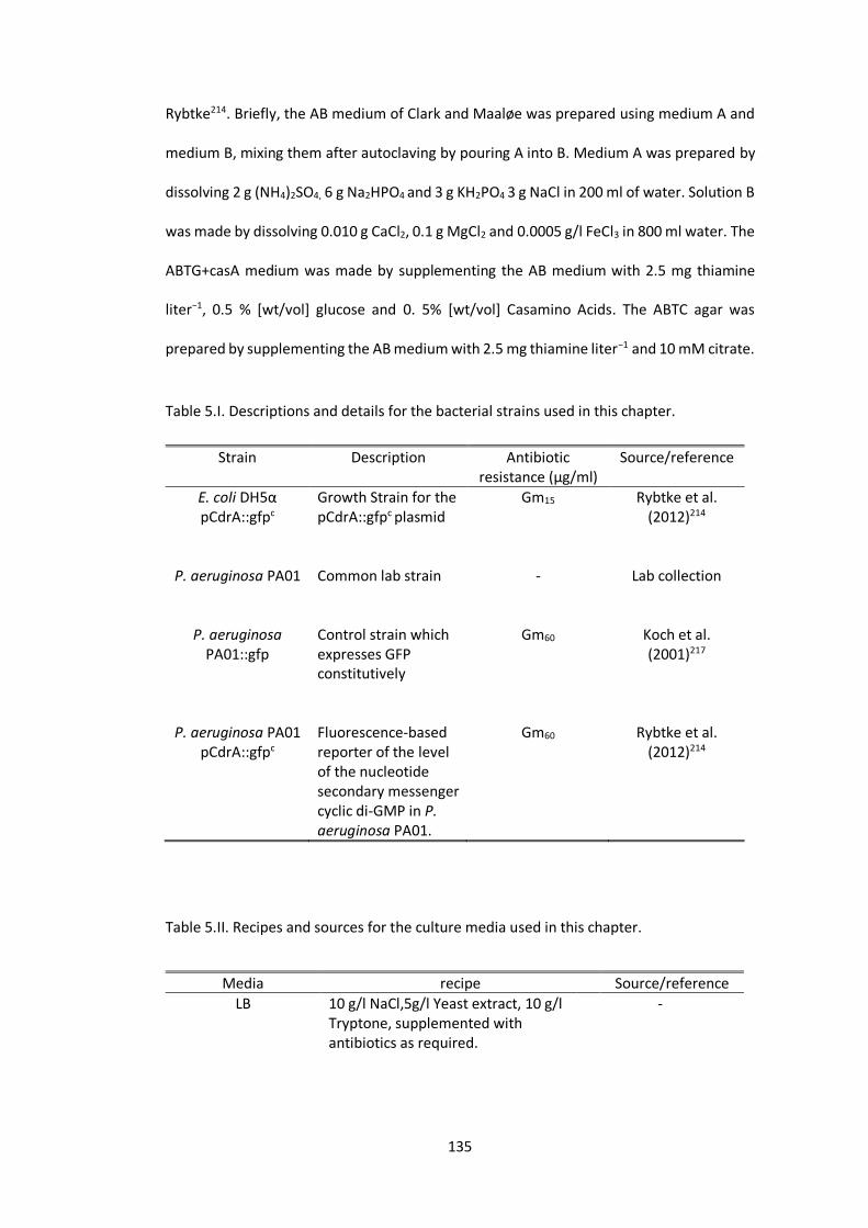
135
Rybtke214. Briefly, the AB medium of Clark and Maaløe was prepared using medium A and
medium B, mixing them after autoclaving by pouring A into B. Medium A was prepared by
dissolving 2 g (NH4)2SO4, 6 g Na2HPO4 and 3 g KH2PO4 3 g NaCl in 200 ml of water. Solution B
was made by dissolving 0.010 g CaCl2, 0.1 g MgCl2 and 0.0005 g/l FeCl3 in 800 ml water. The
ABTG+casA medium was made by supplementing the AB medium with 2.5 mg thiamine
liter−1, 0.5 % [wt/vol] glucose and 0. 5% [wt/vol] Casamino Acids. The ABTC agar was
prepared by supplementing the AB medium with 2.5 mg thiamine liter−1 and 10 mM citrate.
Table 5.I. Descriptions and details for the bacterial strains used in this chapter.
Strain Description Antibiotic resistance (µg/ml)
Source/reference
E. coli DH5α pCdrA::gfpc
Growth Strain for the pCdrA::gfpc plasmid
Gm15 Rybtke et al. (2012)214
P. aeruginosa PA01
Common lab strain
- Lab collection
P. aeruginosa PA01::gfp
Control strain which expresses GFP constitutively
Gm60 Koch et al. (2001)217
P. aeruginosa PA01 pCdrA::gfpc
Fluorescence-based reporter of the level of the nucleotide secondary messenger cyclic di-GMP in P. aeruginosa PA01.
Gm60 Rybtke et al. (2012)214
Table 5.II. Recipes and sources for the culture media used in this chapter.
Media recipe Source/reference
LB 10 g/l NaCl,5g/l Yeast extract, 10 g/l Tryptone, supplemented with antibiotics as required.
-

136
LB agar 10 g/l NaCl,5 g/l Yeast extract, 10 g/l Tryptone, 15 g/l agar, supplemented with antibiotics as required.
-
TSB 30 g/l Tryptone Soya Broth supplemented with antibiotics as required.
-
TSA 30 g/l Tryptone Soya Broth, 15 g/l agar, supplemented with antibiotics as required.
-
1 % TSB 10 g/l Tryptone Soya Broth supplemented with antibiotics as required.
-
ABTG+casA 2 g/l (NH4)2SO4, 6 g/l Na2HPO4, 3 g/l KH2PO4 3 g/l NaCl, 0.010 g/l CaCl2, 0.1 g/l MgCl2, 0.0005 g/l FeCl3, 0.0025 g/l thiamine, 5 g/l glucose and 5 g/l Casamino Acids, supplemented with antibiotics as required.
(AB media) Clark and
Maaløe218
(ABTG+casA)Rybtke214
ABTC agar 2 g/l (NH4)2SO4, 6 g/l Na2HPO4, 3 g/l KH2PO4 3 g/l NaCl, 0.010 g/l CaCl2, 0.1 g/l MgCl2, 0.0005 g/l FeCl3, 0.0025 g/l thiamine, 2g/l citrate, 15 g/l agar, supplemented with antibiotics as required.
(AB media) Clark and Maaløe218
(ABTC agar)Rybtke214
To prepare an overnight culture, cells were freshly streaked onto the relevant
media plates from glycerol stocks two days before the experiment and incubated at 37oC
overnight. The next day 10 ml of the relevant medium in a glass universal was inoculated
with a single colony. The inoculum was then incubated and shaken at 200 rpm at 37oC
overnight (until OD600 ≈ 2). The optical density of cells was measured using a
spectrophotometer (Labtech).
5.3.2 The c-di-GMP reporter PA01 pCdrA::gfpc and the GFP control
strain PA01:gfp

137
PCdrA-gfpc was a gift from Tim Tolker-Nielsen (Addgene plasmid #111614)214.
PCdrA::gfpc uses the cdrA promoter fused with the artificial optimized ribosomal binding
site (RBSII) and GFP as a reporter of c-di-GMP levels in P. aeruginosa (PcdrA-RBSII-
gfp(mut3)-T0-T1). This gene cassette was inserted into the shuttle vector pUCP22Not
(Figure 5.2).
PA01:gfp was used as a control strain. It expresses GFP constitutively (it is produced
in relatively constant amounts regardless of environmental conditions) from miniTn7-based
chromosomal insertion. The chromosomal insertion was driven via miniTn7 expressing
gentamycin and chloramphenicol resistance expressing GFP from the PA1//04/03 promoter.
Figure 5.2. Sequence map of pCdrA::gfpc. (a) Addgene full sequence map for pCdrA::gfpc
created with SnapGene. Shown on the map are: unique 6+ cutters, primers, features and

138
translations. (b) Schematic showing the horizontal cassette map for pCdrA::gfpc showing
the cdrA promoter fused with the artificial optimized ribosomal binding site (RBSII). The
transcriptional fusion is followed by two transcriptional terminators (T0 and T1).
5.3.3 Transformation of pCdrA::gfpc into P. aeruginosa PA01 by
electroporation
PCdrA::gfpc was gifted in E. coli DH5α as an agar stab (from Tom Tolker-Nielson).
The E. coli DH5α pCdrA::gfpc was streaked onto LB agar (containing Gm15) and incubated at
37oC overnight. The next day a single colony was inoculated into 10 ml of LB mixed with
Gm15, which was incubated at 37oC and shaken at 200 rpm overnight. The PCdrA::gfpcc
plasmid was extracted from DH5α using the standard QIAGEN Plasmid protocol (see
Appendices for full protocol).
The plasmid DNA concentration and purity were checked using a Nanodrop ND-
1000 ultraviolet (UV) spectrophotometer (Labtech). Having confirmed the plasmid
preparation was successful, it was transformed into competent P. aeruginosa PA01 by
electroporation. P. aeruginosa cells were made electrocompetent using a sucrose
microcentrifuge-based procedure, following the protocol of Choi et al. 219. An overnight
culture of P. aeruginosa was grown in 6 ml of LB as described previously. This culture was
then separated into 4 different 1.5 ml Eppendorf tubes before the cells were harvested by
centrifugation at 22°C for 2 mins at 16,000 g. The cell pellet in each tube was washed twice
with 1 ml of 300 mM sucrose and the 4 cell pellets were then resuspended in a combined
total of 100 µl of 300 mM sucrose.
For electroporation, 500 ng of the prepared pCdrA::gfpc plasmid was mixed with
100 µl of electrocompetent cells and this mixture was transferred to a 2 mm gap width
electroporation cuvette (Bio-rad). The electroporation was performed at: 25 AF; 200 V; 2.5
kV, using a Bio-Rad GenePulserXcellk. Following electroporation, 1 ml of 22°C LB medium

139
was added at once and cells were transferred to a 1.5 ml Eppendorf. The cells were
incubated at 37°C and shaken at 200 rpm for 1.5 hrs. The cells were then harvested, by
centrifugation at 22°C for 2 min at 16,000 g and 900 µl of the supernatant was discarded.
The cell pellet was then resuspended in the remaining medium. The entire mixture was
then plated on LB with Gm60 plates. The plates were then incubated at 37°C overnight.
Controls included cells pulsed without the added plasmid. The next day a single colony was
inoculated into 10 ml of LB, which was incubated at 37oC and shaken at 200 rpm overnight.
In order to confirm successful transformation of pCdrA::gfpc into P. aeruginosa PA01, the
plasmid was extracted from P. aeruginosa PA01 using the modified QIAGEN Plasmid
protocol (detailed in the Appendices) and the concentration and purity was checked using
a Nanodrop ND-1000 ultraviolet (UV) spectrophotometer (Labtech).
The whole and digested extracted plasmid were analysed using agarose gel
electrophoresis. The plasmid was digested with 1 µl Xba1 and 1 µl HindIII restriction
enzymes (BioLabs) added to 7 µl of plasmid, 2 µl of 10x CutSmart Buffer (BioLabs) and 9 µl
of Milli-Q water and incubated at 37°C for 1.5 hrs. A 1 % w/v agarose gel was made by
dissolving 0.5 g agarose into 50 ml TAE buffer (40 mM Tris-acetate pH 7.7, 1 mM EDTA). The
gel was added to 0.5 µl of ethidium bromide (Sigma) and added to the gel holder before it
set. The holder was then placed in the gel electrophoresis system (ThermoFisher). The
samples were loaded and then run alongside a 1Kb HyperLadder (Bioline) at 110 V DC. The
samples were compared to the ladder using a UV transilluminator (UVIpro Silver, UVItec)
to determine their size. Finally, P. aeruginosa PA01 pCdrA::gfpc was tested using the SNP
fluorescence plate reader assay.
5.3.4 Plate reader assay

140
Microtiter plate-based assays were carried out following the protocol of Rybtke214.
Experiments testing P. aeruginosa PAO1 pCdrA::gfpc as a reporter of c-di-GMP levels using
SNP (Sodium nitroprusside) cells used ABTC agar and ABTG+casA medium. Other
experiments measuring the effect of H202 on c-di-GMP levels cells were conducted using
TSA and 1 % TSB medium.
Overnight inoculums were diluted to OD600 ≈ 0.03 in 30 ml of fresh medium. For
H202 assays, 250 μl of the culture was immediately added to the wells of the microtiter. For
SNP assays the growth was measured manually until OD600 ≈ 0.4, at which point 250 μl of
the cell culture was added to the microtiter wells. After the black-welled, clear bottomed,
96-well Corning microtiter plate was filled, it was incubated in a BioTek Synery HT plate
reader heated to 37°C and set up to measure OD450/OD600 and green fluorescence (arbitrary
GFP units) every 30 min. The plates were shaken in an orbital pattern (3-mm diameter) at
normal speed for 10 min before and after each round of measurements to optimize growth.
The SNP (Sigma) was prepared in 2-fold serial dilutions starting from 250 μM SNP
from a 50 mM stock of SNP dissolved in Milli-Q water. The H202 (Sigma) was prepared in
serial dilutions from a 1 mM stock dissolved in Milli-Q water.
5.3.5 Cell preparation for single cell fluorescence microscopy
Following overnight culture in TSB, as previously described, fresh 1 % TSB medium
with relevant antibiotics was reinoculated 1:10 with the overnight culture and grown with
shaking at 200 rpm at 37°C until the cells reached mid-exponential phase (OD600 ≈ 0.5). This
cell culture was then diluted to OD600 ≈ 0.05 using fresh 1 % TSB medium. Agarose
microscope slides were prepared following an adapted version of the protocol of Jong et al.

141
(2011)105 as described previously in Chapter 4 (Section 4.3.2). These slides were prewarmed
for at least an hour prior to imaging to avoid issues arising from drifting.
5.3.6 Microscope set-up
The microscope slides were mounted on an Olympus IX-71 inverted microscope
with an Olympus UPAON 100XOTIRFM (NA 1.49) immersion oil and TIRF objective lens.
Brightfield images were acquired using an LED (525 nm) which was focused onto the sample
using a condenser lens. For fluorescence imaging, the sample was illuminated with an OBIS
405LX or OBIS 488LX laser. Time lapse images were recorded using an ORCA-Flash4.0 LT
PLUS Digital CMOS camera (C11440-22CU).
5.3.7 Fluorescent dyes and GFPs
ThT is commonly used to stain amyloid fibres96, however, its positive charge also
allowed it to be used as a Nernstian voltage indicator85–87. ThT was supplied by Sigma-
Aldrich. Fresh 2 mM stocks were made up on the day of the experiment and added to the
cells and media at a final working concentration of 10 µM. ThT can be excited at 405 nm,
allowing it to be used in conjunction with 405 nm light treatment. Both the fluorescent
reporter (PCdrA::gfpc) and the constitutively firing GFP control strain (PA01::gfp) contained
the mut3 variation of GFP which was excited using the 488 nm laser.
5.3.8 405 nm light treatment and photobleaching using 488 nm light

142
To treat cells with 405 nm light an OBIS 405LX laser with an irradiance of 120
µW/cm2 was focused on to the surface of the microscope slide. Time lapse images were
acquired every 1 secs.
Cells were photobleached using an OBIS 488LX laser at an irradiance of 120 µW/cm2
and time lapse images were acquired every 6 secs.
5.3.9 Irradiance/dose measurements
The optical power was measured at the sample using a Thorlabs PM121D digital
power meter. The power across the area in which measurements were conducted was
uniform and so the irradiance was given by,
𝐼 =𝑃
𝐴 , (5.1)
where 𝐼 is the irradiance, 𝑃 is the power at the sample and 𝐴 is the illumination area and
the dose (D) in J/cm2 was given by,
𝐷 =𝐼𝑡
1000
(5.2)
where I is the irradiance in mw/cm2 and t is the time of illumination in s.
5.3.10 Data analysis
The data from the plate reader assays was exported to Matlab (MathWorks), where
custom made scripts were used to analyse it. This included the subtraction of the signal due
to background media, averaging over repeats and calculating ratios. All experiments
included at least three repeats with three biological triplicates.

143
The image analysis for the microscopy experiments was conducted using Image J
and Matlab (MathWorks). Background subtraction was done using the ImageJ (National
Institutes of Health) ‘rolling ball’ background plugin with a radius of 4 – 8 µm depending on
the experimental conditions. To obtain fluorescence curves the fluorescence was measured
using the ‘plot Z axis’ function on the ImageJ image analysis toolbox. Signal processing was
performed in Matlab, including signal smoothing using a cubic weighted Savitzky-Golay
filter, which removed additional noise. The average fluorescence per cell was calculated by
averaging the mean fluorescence per cell from at least 20 cells across at least five different
experiments. Origin was used to fit fluorescence curves, to perform the statistical analysis
and for graph plotting. All the errors presented are standard errors.
5.4 Results
5.4.1 Confirming the suitability of P. aeruginosa PAO1 pCdrA::gfpc as a
reporter of c-di-GMP levels
The fluorescence-based reporter P. aeruginosa PA01 pCdrA::gfpc was used to
monitor c-di-GMP levels. This biosensor was originally developed by Rybtke et al. (2012)
who demonstrated its success in detecting an increase in c-di-GMP levels in response to
SNP in P. aeruginosa PAO1 ΔwspFΔpelΔpsl/pCdrA::gfpc 214. This strain was used due to the
higher levels of fluorescence observed, but it is not suitable for biofilm studies, as
wspF/pel/psl are required for biofilm growth. Subsequent studies have used the wild type
P. aeruginosa PAO1 pCdrA::gfpc strain to gauge the levels of c-di-GMP in planktonic and in
biofilm cells220,221.

144
The original experiments of Rybtke were repeated and their results for PAO1
ΔwspFΔpelΔpsl/pCdrA::gfpc were reproduced for PAO1 pCdrA::gfpc (Figure 5.3), confirming
that PAO1 pCdrA::gfpc could be used to successfully gauge the levels of c-di-GMP.
Figure 5.3. Treatment of P. aeruginosa PAO1 pCdrA::gfpc with SNP at concentration of 0
µM, 62.5 µM and 125 µM. (a) Growth measurements given by the OD450. (b) Fluorescence
GFP measurements.
5.4.2 Changes in c-di-GMP levels in response to 405 nm light

145
Fluorescence microscopy was used to dynamically monitor the intracellular c-di-
GMP levels of individual cells treated with 405 nm light. Cells were grown on agarose pad
microscope slides (Section 5.4.5). GFP is photobleached by 405 nm light. It was therefore
not possible to take GFP measurements immediately following 405 nm light treatment, but
it was possible to measure the GFP following recovery. Figure 5.4 shows that after one hour
of recovery that the GFP fluorescence of PA01 pCdrA::gfpc increased, but not back to the
original intensity. Following the same treatment the GFP fluorescence of the constitutively
firing PAO1::gfp strain showed no recovery. This indicates that the continued decreases in
GFP fluorescence following recovery were not reflective of decreases in c-di-GMP levels,
but were instead caused by decreases in the promoter/translator capabilities of GFP or due
to GFP quenching. To probe the mechanism/s responsible for the decreased fluorescence,
I photobleached the GFP. The GFP photobleaching (𝐼(𝑡)) by 488 nm light (at a set irradiance
of 120 ± 2 µW/cm2) was well described by a monoexponential of the form,
𝐼(𝑡) = 𝐼0𝑒−𝑡𝜏
(5.3)
where 𝐼0 is the unbleached GFP fluorescence intensity and 𝜏 is the photobleaching decay
time constant.
The value of 𝐼0 decreased for both PA01 pCdrA::gfpc and PAO1::gfp, but 𝜏 did not
change significantly (Figure 5.4(b)). Before treatment with 405 nm light the GFP
photobleaching time constant of PA01 pCdrA::gfpc was 0.58 ± 0.07 min and after treatment,
it was 0.55 ± 0.03 min. The photobleaching time constant of PAO1::gfp was 0.75 ± 0.07 min
before treatment and 0.71 ± 0.05 min after treatment. The observed decrease in
fluorescence, but maintenance of photobleaching kinetics, is the expected consequence of
photobleaching alone. It is possible that a static quencher may also be acting, but the
maintenance of 𝜏 rules out dynamic quenching following treatment with 3.6 mJ/cm2 of 405
nm light90,92.

146
Figure 5.4. Treatment of P. aeruginosa PAO1 pCdrA::gfpc and P. aeruginosa PAO1::gfp with
405 nm light. (a) Normalised GFP fluorescence per cell before, following and an hour after
treatment of cells with 3.6 mJ/cm2 of 405 nm light. (b) Photobleaching curves for P.
aeruginosa PAO1 pCdrA::gfpc exposed to 488 nm light at an irradiance of 120 ± 2 µW/cm2
(black) before and (red) after treatment with 3.6 mJ/cm2 of 405 nm light, with exponential
fits given by Equation 5.3.
5.4.3 Changes in c-di-GMP levels in response to H202
As it was not possible to measure the c-di-GMP changes in response to 405 nm
light, the changes accompanying H202 oxidative stress were measured. Figure 5.5 shows the
results of plate reader assays in which P. aeruginosa PA01 pCdrA::gfpc , P. aeruginosa
PAO1::gfp and P. aeruginosa PAO1 were grown in the presence of 1 mM H202. At this
concentration the growth of PA01 pCdrA::gfpc and PAO1::gfp were affected, while the
growth of PA01 WT was not (Figure 5.5(b)). The growth of PAO1::gfp was slower than PA01
pCdrA::gfpc and the addition of H202 had a larger impact on the growth of P. aeruginosa
PAO1::gfp.

147
Figure 5.5. Treatment of P. aeruginosa with 1 mM H202. (a) Ratios of the average GFP
fluorescence to OD600 as a function of time since inoculation for: P. aeruginosa PAO1
pCdrA::gfpc (▲), P. aeruginosa PAO1::gfp (■) and P. aeruginosa PAO1 (●), without H202
(black) and with 1 mM H202 (red). (b) Growth curves of: P. aeruginosa PAO1 pCdrA::gfpc
(▲), P. aeruginosa PAO1::gfp (■) and P. aeruginosa PAO1 (●), without H202 (black) and with
1 mM H202 (red). (c) Ratio of average GFP fluorescence to OD600 , at mid-exponential growth
phase (OD600 ≈ 0.5), without H202 (blue) and with 1 mM H202 (green) for: P. aeruginosa PAO1

148
pCdrA::gfpc (▲), P. aeruginosa PAO1::gfp (■) and P. aeruginosa PAO1 (●). The presented
errors are standard errors.
Figure 5.5(a) shows the ratio of GFP fluorescence to growth (given by the optical
density (OD600)). At all stages of growth the GFP/ OD600 ratio of PA01 pCdrA::gfpc was larger
when grown in the presence of 1 mM H202. The GFP/ OD600 of PA01 pCdrA::gfpc increased
over 10 hrs of growth, with comparable increases observed when grown in the presence of
H202. The ratios of the background GFP fluorescence and autofluorescence to OD600 (given
by P. aeruginosa PAO1::gfp and PA01 WT respectively) decreased over 10 hrs of growth,
with both ratios showing comparable changes when grown in the presence of H202. Because
of the differences in the growth rates, the GFP/ OD600 values at mid-exponential growth
phase (OD600 ≈ 0.5) were compared (Figure 5.5(b)). The GFP/ OD600 of PA01 pCdrA::gfpc was
larger when 1 mM of H202 was added. In contrast, the ratio was lower in both P. aeruginosa
PAO1::gfp and PA01 WT upon addition of H202. This indicates that the increases seen in
PA01 pCdrA::gfpc were caused by an increase in the c-di-GMP levels, due to the addition of
low levels of H202.
It was not possible to conduct ThT measurements in the plate reader and so in
order to conduct parallel membrane potential and c-di-GMP measurements fluorescence
microscopy was used. Sessile cells are known to have a higher tolerance to H202 than
planktonic cells. We, therefore measured the response of cells on the agar microscopy
slides to a range of H202 concentrations between 1 μm – 10 mM. Figure 5.6(a) shows that
addition of 1 μm – 1 mM H202 did not significantly affect the average GFP fluorescence of
PA01 pCdrA::gfpc cells at the 5 % significance level. However, addition of >1 mM H202
significantly decreased the fluorescence. These results were mirrored in the control strain
PAO1::gfp, suggesting that these results were not caused by changes in the levels of c-di-
GMP. Photobleaching of the GFP using a 488 nm laser was faster (smaller 𝜏 in Equation 5.3)

149
at the higher H202 concentrations (Figure 5.6(b)). Faster bleaching was observed from 1 mM
H202 in PA01 pCdrA::gfpc and after 1 mM in PAO1::gfp.
Figure 5.6. Treatment of P. aeruginosa PA01 pCdrA::gfpc and P. aeruginosa PA01::gfp with
H202. (a) Average cell GFP fluorescence of P. aeruginosa PA01 pCdrA::gfpc and P. aeruginosa
PA01::gfp, for a range of H202 concentrations (1 µM, 10 µM, 1 mM and 10 mM), normalised
to the average cell GFP fluorescence without H202. (b) The normalised average cell decay
time constant of photobleaching by 120 ± 2 µW/cm2 488 nm light (Equation 5.3) as a
function of H202 concentration. The inset shows the decrease in cell fluorescence due to
addition of 10 mM H202 in fluorescence microscopy images. The presented errors are
standard errors.
5.4.4 Membrane potential response to H202
Previous ThT experiments (detailed in Chapter 4) were repeated in the presence of
H202. The average cell ThT fluorescence (averaged over at least 20 cells across at least five
different experiments) was significantly higher in the presence of 10 mM H202 (Figure
5.7(a)). Treatment with 405 nm light produced previously described membrane
hyperpolarisations, but these occurred at a faster rate in the presence of H202 (Figure
5.7(b)). Overall this suggests that P. aeruginosa hyperpolarises in response to H202 and that

150
the combination of H202 and 405 nm light is synergistic causing a larger oxidative stress and
so a faster hyperpolarisation response.
Figure 5.7. Membrane potential response of P. aeruginosa treated with H202. (a) Change in
average ThT fluorescence per cell caused by addition of 10 mM H202. (b) Average normalised
ThT (membrane potential) dose response without H202 (black) and with 10 mM H202 (red) in
response to 120 µW/cm2 405 nm light. The presented errors are standard errors.
5.5 Discussion
Biofilm growth relies on the coordination of behaviour between its constituent
bacteria; this is achieved via a complex network of signalling molecules and genetic cues.
The secondary messenger c-di-GMP is a crucial regulator in biofilm growth in a range of
bacterial species.
Recent studies have revealed that 405 nm light induces photophysiological
responses in a range of bacteria via different blue-light receptor classes (LOV, BLUF and
PYP)197,198 as described in the previous chapter (Section 4.5) The motility of Synechocystis
sp. PCC 6803 is affected by 405 nm light via an cyclic diguanylate (c-di-GMP) signal
transduction system204. P. aeruginosa has been shown to regulate behaviour in response to

151
light202 and regulates stress via c-di-GMP/cAMP levels205. The majority of diguanylate
cyclases (DGCs) and phosphodiesterases (PDEs) that have been identified in the genome of
P. aeruginosa still remain uncharacterized43. One hypothesis is that 405 nm light stimulates
the production of one or more of these PDEs, ultimately resulting in lower levels of c-di-
GMP and cell dispersal.
Unfortunately, it was not possible to measure the c-di-GMP levels following 405 nm
light treatment and so were unable to fully test this hypothesis. This was partly due to GFP
photobleaching, but was mainly because the GFP fluorescence was fundamentally affected
by the 405 nm light. The levels of c-di-GMP following recovery after photobleaching were
measured and it was found that the control strain which produced GFP constitutively did
not recover. In order to investigate what caused the GFP fluorescence decreases following
405 nm light treatment, the sample was photobleached using 488 nm light. The observed
decrease in fluorescence was not accompanied by a change in photobleaching kinetics. This
is the expected consequence of photobleaching alone. It is possible that a static quencher
may also be acting, but the maintenance of photobleaching kinetics rules out dynamic
quenching following treatment with 3.6 mJ/cm2 of 405 nm light90,92. Treatment of cells with
H202 affected the kinetics of photobleaching. We therefore suggest that the decreases in
fluorescence induced by 405 nm light were not caused by the quenching of GFP
fluorescence via ROS, or more specifically H202 (the main ROS produced by bacteria in
response to 405 nm light171). It is, however, possible that the photooxidative stress induced
by 405 nm light affected the promoter/translator capabilities of GFP. In the future, it may
be possible to test this hypothesis by using a fluorescence-based reporter which uses an
alternative fluorescent protein. The reporter strain PA01 pCdrA::gfpc contains GFPmut3,
which is more sensitive to photobleaching than some other fluorescent proteins216.
However, other fluorescent proteins may be unsuitable for alternative reasons, for
example, eGFP can induce high levels of oxidative stress in cells222. For future work the

152
development of a c-di-GMP reporter strain with a red fluorescent protein would be
useful223.
The levels of H202 required to elicit a response from adhered P. aeruginosa PA01
cells altered the GFPmut3 fluorescence and so our reporter could not be used. The decrease
in GFP fluorescence observed in response to > 1 mM of H202 was dynamic and decreased in
a time dependant manner when the sample was photobleached by 488 nm light. Exposure
to light can induce ROS production and the presence of a fluorescent protein that absorbs
the excitation light enhances ROS production224. If ROS was causing the fluorescence
quenching of GFP, the production of additional ROS could explain the time dependant
changes in fluorescence. This indicates that fluorescence imaging of GFPs in the presence
of ROS may induce significant ROS production, which may not only render the GFP
ineffective as a reporter of specific gene transcription but could also induces changes in cell
behaviour. Recent studies have shown that fluorescent proteins, such as eGFP, can induce
catalytic oxidative stress in biological systems222.
Also, of concern was the effect of GFP production on oxidative stress resilience. Our
control strain (P. aeruginosa PA01::gfp) had a larger GFP fluorescence than our reporter
strain (P. aeruginosa PA01 pCdrA::gfpc) and it was more sensitive to oxidative stress. Its
recovery was slower following 405 nm light treatment and its growth was more greatly
affected by H202. The growth of both the strains expressing GFP were slowed by the
addition of H202, whereas the wild type PA01 remained unaffected.
Taken together, these results demonstrate that GFP reporters may not be suitable
for systems with high levels of ROS. This is an important result for future studies and
highlights the importance of using a constitutively firing GFP strain as a control. Previous
studies have not always used such controls, but our results demonstrate the need to do so.
Excitation at longer wavelengths generally incurs less ROS production and damage than

153
excitation at equivalent irradiances with a shorter wavelength224,225. It would, therefore, be
interesting to develop a reporter strain which is based on a fluorescent protein that is
excited at a longer wavelength (e.g. red) and to test whether it performs better in the
presence of ROS.
Planktonic P. aeruginosa PA01 cells have a lower tolerance to H202 than biofilm
cells226,227. It was therefore possible to use a plate reader assay to study the effect of ROS
(caused by H202) on the c-di-GMP levels of cells. At lower levels of H202, where growth was
only minimally affected, the H202 stimulated an increase in the levels of intracellular c-di-
GMP. It is not possible to conduct membrane potential (ThT) measurements in the plate
reader assay and so it was not possible to directly connect these results with changes in the
membrane potential. However, via fluorescence microscopy, it was possible to study how
ROS affected the membrane potentials of surface adhered P. aeruginosa PA01 cells. The
addition of 10 mM H202 caused membrane potential hyperpolarisations and the addition of
H202 increased the rate of the previously described 405 nm light induced membrane
potential hyperpolarisations.
In summary, it was not possible to test the hypothesis that the cell dispersal and
membrane potential hyperpolarisations that were observed in response to photooxidative
stress were associated with changes in the levels of intracellular c-di-GMP levels. However,
it was possible to show that at low levels oxidative stress can induce increases in the levels
of c-di-GMP. This indicates that P. aeruginosa does regulate ROS stress via this intracellular
messenger.

154
5.6 Conclusions
The GFP-based fluorescent reporter P. aeruginosa PA01 pCdrA::gfpc was used to
investigate the role c-di-GMP levels play in the regulation of the photooxidative stress
response of P. aeruginosa to 405 nm light. The photooxidative stress induced changes in
the GFP and therefore PA01 pCdrA::gfpc could not be reliably used to measure the c-di-
GMP levels. Photobleaching kinetics were used to understand the mechanisms causing the
reduction in GFP fluorescence. It was found that the decreases were caused by decreases
in the expression of the GFP (due to different promoter/translator capabilities) and/or due
to static GFP quenching. Oxidative stress, in the form of H202, also directly affected the GFP
fluorescence. Our results suggest that 488 nm light (the wavelength used for excitation and
imaging of GFP) added to the oxidative stress.
Our results also suggest that strains which produce a larger quantity of GFP are more
sensitive to oxidative stress. The two key requirements of a successful fluorescence-based
biosensor are that the levels of fluorescence are reflective of the gene expression of interest
and that the sensing mechanism (in this case GFP expression) does not affect the cells. It
was found that both these requirements were not met by the GFPmut3-based reporter in
environments with oxidative stress > 1 mM H202.
At lower levels of oxidative stress the c-di-GMP levels were faithfully reported by
PA01 pCdrA::gfpc and it was possible to show that c-di-GMP levels were raised in response
to H202. Therefore, the oxidative stress response of P. aeruginosa PA01 was regulated by c-
di-GMP. At higher levels, it has been shown that H202 can induce dispersal of P. aeruginosa
via c-di-GMP. I therefore hypothesize that c-di-GMP regulates the observed dispersal
response of PA01 to 405 nm light and more broadly that intracellular c-di-GMP levels are
connected to the cell’s membrane potential. In the future, it may be possible to investigate

155
this using a fluorescence-based c-di-GMP reporter which uses an alternative fluorescent
protein.

156
6 Conclusions
Fluorescence microscopy was combined with mathematical techniques to
investigate the role membrane potentials play in the stress response of bacteria and in
bacterial communication. It recently emerged that bacteria in biofilms use electrical signals
to communicate85. Such universal mechanisms of communication offer particularly
attractive targets to develop treatments, as they may offer a widespread solution.
In order to understand the new class of active excitable matter that is bacterial
biofilms, it may be possible to learn from the well-established field of eukaryotic excitable
matter. We have demonstrated how new methods of data analysis and agent-based
modelling may be used to investigate electrical signalling in bacterial biofilms. These
methods were used to describe newly observed phenomena in the electrical signals of
circular B. subtilis biofilms. Centripetal electrical wavefronts, which travelled inward from
the edge of a circular biofilm were described for the first time. Moments’ analysis was used
to rigorously quantify these signals, as well as previously described centrifugal signals. This
new method of analysis revealed that, contrary to previous belief, the electrical signals did
not propagate constantly through the biofilm. The centrifugal wavefront travelled slower
than the centripetal wavefront, demonstrating that the curvature of the biofilms affected
the signal propagation, in agreement with theoretical predictions165. Also, in contradiction
to prior belief, it was found that the fluorescence energy density and the amplitude of
wavefronts decreased with distance from the biofilm centre.
An agent-based fire-diffuse-fire (ABFDF) model was used to show that the
arrangement of cells and curvature alone were enough to explain the key characteristics of
electrical wave propagation. However, some of the subtler characteristics of signal
propagation were not predicted by our ABFDF model. In the future it may be possible to
also explain these characteristics by adding more specific details of biofilm growth (e.g.

157
growth of bacteria in chains) to the current model. In nature, biofilms form complex, three-
dimensional structures so another extension to this project would involve studying
electrical signalling in three-dimensional biofilms. This is expected to be significantly more
challenging. The exact origin of the centripetal wavefronts remains elusive. This could be
investigated by studying B. subtilis deletion strains (e.g. yugO deletion) under varying
environmental conditions.
Charge transfer through a biofilm defines its electrical properties and is thus an
important consideration when studying electrical fluctuations and potentials. The diffusion
of charged and uncharged molecules through a biofilm is dependent on the structure and
composition of the EPS. For example, Geobacter sulfurreducens, an electricigen, produces
protein filaments which increase the efficiency of long-range electron transport228. The
composition and structure of a B. subtilis biofilm varies depending on the experimental
conditions20,51 (Section 1.2). The structure and composition of the circular B. subtilis biofilms
studied has not yet be quantified. In the future the biofilms’ fine structure may be resolved
via super-resolution microscopy, which can overcome the diffraction limit of traditional
techniques while still maintaining the native structure. In order to build an initial picture of
the biofilms’ structure, experiments which label the key components of B. subtilis biofilms
should be possible following the protocols summarised in the review by Schlafer & Meyer
(2015)229. For example, TasA protein fibres can be labelled using established protocols
which use Thioflavin-T or Congo red57.
New photodynamical therapies seek to use 405 nm light due to its intrinsic
antimicrobial effect171,199,230. The role membrane potentials play in the response of bacteria
to 405 nm light was investigated. Membrane potential hyperpolarisations were observed
in both the Gram-negative bacterium P. aeruginosa and the Gram-positive bacterium B.
subtilis. This was the first time that photo-induced membrane potential hyperpolarisations
were observed in bacteria. At the early stages of biofilm growth cells dispersed and/or were

158
physically altered by the 405 nm light. Residence probabilities provided a robust statistical
tool to quantify cell dispersal.
The photophysical and the membrane potential dose response were both
dependant on the stage of biofilm growth. The membrane potential dose response was
2.91 ± 0.02 times less steep in mature biofilm cells than in initially adhered cells. A non-
linear Hodgkin-Huxley model was used to explore differences in the observed responses.
These results provide new insight into the involvement of membrane potentials in the
photoresponse of bacteria.
One possible extension to this work would involve measuring the levels of reactive
oxygen species using either a ROS dye or a fluorescence-based reporter strain. Two
fluorescence-based reporter dyes, 6-carboxy-2',7'-dichlorodihydrofluorescein diacetate
(carboxy-H2DCFDA) and hydroxyphenylfluorescein (HPF), are commonly used to directly
measure ROS production in bacteria231,232. The reliability of these dyes has been called in to
question231,233,234. These dyes also cannot be used to dynamically measure ROS levels in
biofilms as the preparation technique requires cells to be washed before a single
measurement is taken. Therefore, these dyes cannot be used to conduct ROS
measurements alongside the current measurements and a fluorescence-based reporter
would be more suitable. We conducted initial experiments using the protein-based sensors
HyPer and SypHer. HyPer can be used to measure intracellular H202 levels and SypHer can
be used as a HyPer-control and pH sensor235. Unfortunately, HyPer and SypHer were both
photobleached by the 405 nm light and so it was not possible to use them to measure the
effect of the light. In the future it may be possible to develop a fluorescence-based reporter
which operates at different wavelengths so that such experiments can be carried out.
Another possible extension would involve studying the response of bacteria treated
with a 405 nm light-emitting diode (LED) array171,230,236. This would allow comparison
between laser and LED light, which initial studies show have comparable antimicrobial

159
efficacies237, as well as allowing comparison between planktonic and biofilm growth. LED
array experiments are also compatible with ROS dyes. In the future it may be possible to
follow previous experiments in which an LED array is used to treat cells grown in a multi-
well plate171. In this study cells were removed from the wells and washed before the ROS
was measured using the fluorescent dye carboxy-H2DCFDA. The fluorescence was
measured using a spectrofluorophotometer. Similar experiments could be performed
alongside measurements of membrane potentials using ThT, to confirm the association
between 405 nm light treatment, ROS and membrane potential hyperpolarisations.
However, the measurement of fluorescence via this method is not as sensitive or accurate
as the methods we have used. It is also possible that the incubation step required for
carboxy-H2DCFDA may introduce a delay long enough to cause hyperpolarisations to be
missed.
Recent studies have revealed that bacteria respond to 405 nm light via designated
blue-light receptors. The motility of Synechocystis sp. PCC 6803 is affected by 405 nm light
via the cyclic diguanylate (c-di-GMP) signal transduction system204. P. aeruginosa has been
shown to regulate behaviour in response to light202 and regulates stress via c-di-
GMP/cAMP levels205. The majority of diguanylate cyclases (DGCs) and phosphodiesterases
(PDEs) that have been identified in the genome of P. aeruginosa still remain
uncharacterized43. One hypothesis is that 405 nm light stimulates the production of one or
more of these PDEs, ultimately resulting in lower levels of c-di-GMP and cell dispersal. To
test this hypothesis the GFP-based fluorescent reporter P. aeruginosa pCdrA::gfpc was used
to measure c-di-GMP levels. Unfortunately the GFP fluorescence was altered by 405 nm
light so pCdrA::gfpc could not be reliably used to measure c-di-GMP. Oxidative stress, in the
form of H202, also directly affected the GFP fluorescence. Our results suggest that 488 nm
light (the wavelength used for excitation and imaging of GFP) as well as GFP production
added to the oxidative stress. These results suggest that in the presence of oxidative stress

160
(H202 > 1 mM) GFP is not a faithful reporter and that the imaging of GFP may induce further
oxidative stress. This is of interest to a wide range of studies which use GFPs99,100 and our
results demonstrate the importance of using a constitutively firing GFP strain as a control.
At lower levels of oxidative stress the c-di-GMP levels were faithfully reported by PA01
pCdrA::gfpc and it was found that c-di-GMP levels were raised in response to H202.
In the future, to test the hypothesis that c-di-GMP is involved in the response of P.
aeruginosa to 405 nm light, a reporter which faithfully reports c-di-GMP levels in the
presence in high levels of oxidative stress is required. It is possible that a reporter strain
based on a fluorescent protein which is excited at a longer wavelength (e.g. red) may be
used223,238. This would involve developing such a reporter and testing its performance
before using it. Once a suitable reporter has been developed it may be possible to
supplement traditional fluorescence microscopy techniques with fluorescence lifetime
imaging (FLIM)239, which produces an image based on the differences in the excited state
decay rate from the sample and can be used to produce more robust results than intensity
based methods.
Further experiments could also be performed using a 405 nm LED array as discussed
above. Following the work of Ramakrishnan et al (2016) a 405 nm LED array could be used
to treat cells in a multi-well plate171. This would allow the fluorescence plate reader
experiments performed for H202 to be conducted using 405 nm light as the stress. This
would allow our hypotheses to be tested further, as well as extending the study to include
different modes of growth.

161
7 Bibliography
1. Blee, J. A., Roberts, I. S. & Waigh, T. A. Spatial propagation of electrical signals in
circular biofilms: A combined experimental and agent-based fire-diffuse-fire study.
Phys. Rev. E 100, 52401 (2019).
2. Blee, J. A., Roberts, I. S. & Waigh, T. A. Membrane potentials, oxidative stress and
the dispersal response of bacterial biofilms to 405 nm light. Phys. Biol. 17, 036001
(2020).
3. Romeo, T. Bacterial biofilms. vol. 322 (Springer Berlin Heidelberg, 2008).
4. Flemming, H.-C., Neu, T. R. & Wozniak, D. J. The EPS matrix: the ‘house of biofilm
cells’. J. Bacteriol. 189, 7945–7947 (2007).
5. Wingender, J. et al. Biofilms: an emergent form of bacterial life. Nat. Rev.
Microbiol. 14, 563–575 (2016).
6. Jacobsen, S. M., Stickler, D. J., Mobley, H. L. T. & Shirtliff, M. E. Complicated
catheter-associated urinary tract infections due to Escherichia coli and Proteus
mirabilis. Clin. Microbiol. Rev. 21, 26–59 (2008).
7. Makhlouf, A. S. H. & Botello, M. A. Failure of the metallic structures due to
microbiologically induced corrosion and the techniques for protection. Handbook
of Materials Failure Analysis (eds. Makhlouf, A. S. H. & Aliofkhazraei, M. B. T.-H. of
M. F. A.) 1–18 (Elsevier, 2018).
8. Høiby, N. et al. The clinical impact of bacterial biofilms. Int J Oral Sci Int. J. Oral Sci.
3, 55–65 (2011).
9. del Pozo, J. L., Rouse, M. S. & Patel, R. Bioelectric effect and bacterial biofilms. A
systematic review. Int. J. Artif. Organs 31, 786–795 (2008).

162
10. Schultz, M. P., Bendick, J. A., Holm, E. R. & Hertel, W. M. Economic impact of
biofouling on a naval surface ship. Biofouling 27, 87–98 (2011).
11. R Robertson, S. & JC McLean, R. Beneficial biofilms. AIMS Bioeng. 2, 437–448
(2015).
12. Yu, Y., Chen, H.-L., Yong, Y.-C., Kim, D. & Song, H. Conductive artificial biofilm
dramatically enhances bioelectricity production in Shewanella-inoculated microbial
fuel cells. Chem. Commun. 47, 12825–12827 (2011).
13. McLoon, A. L., Guttenplan, S. B., Kearns, D. B., Kolter, R. & Losick, R. Tracing the
Domestication of a Biofilm-Forming Bacterium. J. Bacteriol. 193, 2027–2034
(2011).
14. Beyenal, H., Donovan, C., Lewandowski, Z. & Harkin, G. Three-dimensional biofilm
structure quantification. J. Microbiol. Methods 59, 395–413 (2004).
15. Di Martino, P. Extracellular polymeric substances, a key element in understanding
biofilm phenotype. AIMS Microbiol. 4, 274–288 (2018).
16. Hall, C. W. & Mah, T.-F. Molecular mechanisms of biofilm-based antibiotic
resistance and tolerance in pathogenic bacteria. FEMS Microbiol. Rev. 41, 276–301
(2017).
17. Anderl, J. N., Franklin, M. J. & Stewart, P. S. Role of antibiotic penetration limitation
in Klebsiella pneumoniae biofilm resistance to ampicillin and ciprofloxacin.
Antimicrob. Agents Chemother. 44, 1818–1824 (2000).
18. Chich, J.-F. A mini review: proteomic analysis, a post-genomic approach. Lait 81,
13–18 (2001).
19. Fallis, A. . BslA is a self-assembling bacterial hydrophobin that coats the Bacillus

163
subtilis biofilm. J. Chem. Inf. Model. 53, 1689–1699 (2013).
20. Vlamakis, H., Chai, Y., Beauregard, P., Losick, R. & Kolter, R. Sticking together:
building a biofilm the Bacillus subtilis way. Nat. Rev. Microbiol. 11, 157–168 (2013).
21. O’Toole, G., Kaplan, H. B. & Kolter, R. Biofilm formation as microbial development.
Annu. Rev. Microbiol. 54, 49–79 (2000).
22. Garrett, T. R., Bhakoo, M. & Zhang, Z. Bacterial adhesion and biofilms on surfaces.
Prog. Nat. Sci. 18, 1049–1056 (2008).
23. Klemm, P. & Schembri, M. A. Bacterial adhesins: function and structure. Int. J. Med.
Microbiol. 290, 27–35 (2000).
24. Kaplan, J. B. Biofilm dispersal: mechanisms, clinical implications, and potential
therapeutic uses. J. Dent. Res. 89, 205–218 (2010).
25. Wolska, K. I., Grudniak, A. M., Rudnicka, Z. & Markowska, K. Genetic control of
bacterial biofilms. J. Appl. Genet. 57, 225–238 (2016).
26. Hughes, D. T. & Sperandio, V. Inter-kingdom signalling: communication between
bacteria and their hosts. Nat. Rev. Microbiol. 6, 111–120 (2008).
27. Chun, C. K., Ozer, E. A., Welsh, M. J., Zabner, J. & Greenberg, E. P. Inactivation of a
Pseudomonas aeruginosa quorum-sensing signal by human airway epithelia. Proc.
Natl. Acad. Sci. 101, 3587–3590 (2004).
28. Stewart, P. S. & Franklin, M. J. Physiological heterogeneity in biofilms. Nat. Rev.
Microbiol. 6, 199–210 (2008).
29. Keren, I., Kaldalu, N., Spoering, A., Wang, Y. & Lewis, K. Persister cells and
tolerance to antimicrobials. FEMS Microbiol. Lett. 230, 13–18 (2004).
30. Dowds, B. C. A. The oxidative stress response in Bacillus subtilis. FEMS Microbiol.

164
Lett. 124, 255–263 (1994).
31. Madsen, J. S., Burmølle, M., Hansen, L. H. & Sørensen, S. J. The interconnection
between biofilm formation and horizontal gene transfer. FEMS Immunology and
Medical Microbiology vol. 65 183–195 (2012).
32. Orlandi, V. T., Bolognese, F., Chiodaroli, L., Tolker-Nielsen, T. & Barbieri, P.
Pigments influence the tolerance of pseudomonas aeruginosa PAO1 to
photodynamically induced oxidative stress. Microbiol. (United Kingdom) 161,
2298–2309 (2015).
33. Setlow, P. Spores of Bacillus subtilis: Their resistance to and killing by radiation,
heat and chemicals. J. Appl. Microbiol. 101, 514–525 (2006).
34. Jakubowski, W. & Walkowiak, B. Resistance of oxidative stress in biofilm and
planktonic cells. Brazilian Arch. Biol. Technol. 58, 300–308 (2015).
35. Miller, R. V. Study of the Response of a Biofilm Bacterial Community to UV
Radiation. Appl. Environ. Microbiol. 65, 2025–2031 (1999).
36. Svenningsen, N. B., Martínez-García, E., Nicolaisen, M. H., de Lorenzo, V. & Nybroe,
O. The biofilm matrix polysaccharides cellulose and alginate both protect
Pseudomonas putida mt-2 against reactive oxygen species generated under matric
stress and copper exposure. Microbiol. (United Kingdom) 164, 883–888 (2018).
37. Dai, T. et al. Blue light rescues mice from potentially fatal pseudomonas aeruginosa
burn infection: Efficacy, safety, and mechanism of action. Antimicrob. Agents
Chemother. 57, 1238–1245 (2013).
38. Wagner, V. E. & Iglewski, B. H. P. aeruginosa biofilms in CF infection. Clin. Rev.
Allergy Immunol. 35, 124–134 (2008).

165
39. Yu, C., Wu, J., Contreras, A. E. & Li, Q. Control of nanofiltration membrane
biofouling by Pseudomonas aeruginosa using d-tyrosine. J. Memb. Sci. 423–424,
487–494 (2012).
40. Altaf, M. M., Ahmad, I., Khan, M. S. A. & Grohmann, E. Bacillus biofilms and their
role in plant health. Biofilms in Plant and Soil Health 55–67 (John Wiley & Sons,
Ltd, 2017).
41. Benamara, H. et al. Characterization of Membrane Lipidome Changes in
Pseudomonas aeruginosa during Biofilm Growth on Glass Wool. PLoS One 9,
e108478 (2014).
42. Ha, D.-G. & O’Toole, G. A. C-di-GMP and its effects on biofilm formation and
dispersion: a Pseudomonas Aeruginosa review. Microbiol. Spectr. 3, 1–12 (2015).
43. Valentini, M. & Filloux, A. Biofilms and cyclic di-GMP (c-di-GMP) signaling: lessons
from Pseudomonas aeruginosa and other bacteria. J. Biol. Chem. 291, 12547–
12555 (2016).
44. Boyd, C. D. & O’Toole, G. A. Second messenger regulation of biofilm formation:
Breakthroughs in understanding c-di-GMP effector systems. Annu. Rev. Cell Dev.
Biol. 28, 439–462 (2012).
45. Chua, S. L. et al. C-di-GMP regulates Pseudomonas aeruginosa stress response to
tellurite during both planktonic and biofilm modes of growth. Nat. Publ. Gr. 1–13
(2015).
46. Römling, U., Galperin, M. Y. & Gomelsky, M. Cyclic di-GMP: the first 25 years of a
universal bacterial second messenger. Microbiol. Mol. Biol. Rev. 77, 1–52 (2013).
47. Hay, I. D., Remminghorst, U. & Rehm, B. H. A. MucR, a novel membrane-associated
regulator of alginate biosynthesis in Pseudomonas aeruginosa. Appl. Environ.

166
Microbiol. 75, 1110–1120 (2009).
48. Malone, J. G. et al. The structure–function relationship of WspR, a Pseudomonas
fluorescens response regulator with a GGDEF output domain. Microbiology 153,
980–994 (2007).
49. De, N., Navarro, M. V. A. S., Wang, Q., Krasteva, P. V & Sondermann, H. B. T.-M. in
E. Biophysical Assays for Protein Interactions in the Wsp Sensory System and
Biofilm Formation. Methods in Enzymology: Two-Component Signaling Systems,
Part C vol. 471 161–184 (Academic Press, 2010).
50. De, N. et al. Phosphorylation-independent regulation of the diguanylate cyclase
WspR. PLOS Biol. 6, e67 (2008).
51. Marvasi, M., Visscher, P. T. & Casillas Martinez, L. Exopolymeric substances (EPS)
from Bacillus subtilis: Polymers and genes encoding their synthesis. FEMS
Microbiology Letters vol. 313 1–9 (2010).
52. Lundberg, M. E., Becker, E. C. & Choe, S. MstX and a putative potassium channel
facilitate biofilm formation in Bacillus subtilis. PLoS One 8, e60993 (2013).
53. Badri, D. V. et al. Galactose metabolism plays a crucial role in biofilm formation by
Bacillus subtilis. MBio 3, 1–10 (2013).
54. Dogsa, I., Brloznik, M., Stopar, D. & Mandic-Mulec, I. Exopolymer diversity and the
role of levan in Bacillus subtilis biofilms. PLoS One 8, 2–11 (2013).
55. Ghafoor, A., Hay, I. D. & Rehm, B. H. A. Role of exopolysaccharides in Pseudomonas
aeruginosa biofilm formation and architecture. Appl. Environ. Microbiol. 77, 5238–
5246 (2011).
56. Cairns, L. S., Hobley, L. & Stanley-Wall, N. R. Biofilm formation by Bacillus subtilis:

167
New insights into regulatory strategies and assembly mechanisms. Mol. Microbiol.
93, 587–598 (2014).
57. Romero, D., Aguilar, C., Losick, R. & Kolter, R. Amyloid fibers provide structural
integrity to Bacillus subtilis biofilms. Proc. Natl. Acad. Sci. 107, 2230–2234 (2010).
58. Terra, R., Stanley-Wall, N. R., Cao, G. & Lazazzera, B. A. Identification of bacillus
subtilis sipw as a bifunctional signal peptidase that controls surface-adhered
biofilm formation. J. Bacteriol. 194, 2781–2790 (2012).
59. Hentzer, M. et al. Alginate overproduction affects Pseudomonas aeruginosa
biofilm structure and function. J. Bacteriol. 183, 5395–5401 (2001).
60. Ma, L. et al. Assembly and development of the Pseudomonas aeruginosa biofilm
matrix. PLOS Pathog. 5, e1000354 (2009).
61. Friedman, L. & Kolter, R. Genes involved in matrix formation in Pseudomonas
aeruginosa PA14 biofilms. Mol. Microbiol. 51, 675–690 (2004).
62. Koprowski, P. & Kubalski, A. Bacterial ion channels and their eukaryotic
homologues. BioEssays vol. 23 1148–1158 (2001).
63. Saimi, Y., Loukin, S. H., Zhou, X. L., Martinac, B. & Kung, C. Ion channels in
microbes. Methods Enzymol. 294, 507–524 (1998).
64. Treptow, W. & Tarek, M. K+ conduction in the selectivity filter of potassium
channels is monitored by the charge distribution along their sequence. Biophys. J.
91, L81–L83 (2006).
65. Doyle, D. A. The structure of the potassium channel: molecular basis of K+
conduction and selectivity. Science (80-. ). 280, 69–77 (1998).
66. Payandeh, J., Scheuer, T., Zheng, N. & Catterall, W. A. The crystal structure of a

168
voltage-gated sodium channel. Nature 475, 353–358 (2011).
67. Hou, X., Pedi, L., Diver, M. M. & Long, S. B. Crystal structure of the calcium release-
activated Calcium channel Orai. Science (80-. ). 338, 1308–1313 (2012).
68. Sansom, M. S., Shrivastava, I. H., Ranatunga, K. M. & Smith, G. R. Simulations of ion
channels--watching ions and water move. Trends Biochem. Sci. 25, 368–74 (2000).
69. Kuang, Q., Purhonen, P. & Hebert, H. Structure of potassium channels. Cell. Mol.
Life Sci. 72, 3677–93 (2015).
70. Miller, J. B. & Koshland, D. E. Sensory electrophysiology of bacteria: relationship of
the membrane potential to motility and chemotaxis in Bacillus subtilis. Proc. Natl.
Acad. Sci. U. S. A. 74, 4752–6 (1977).
71. Reza, S. N. Mechanosensitive ion channels. Usp. Fiziol. Nauk 33, 29–37 (2002).
72. Edwards, M. D. et al. Characterization of three novel mechanosensitive channel
activities in Escherichia coli. Channels (Austin). 6, 272–281 (2012).
73. Sukharev, S. I., Blount, P., Martinac, B., Blattner, F. R. & Kung, C. A large-
conductance mechanosensitive channel in E. coli encoded by mscL alone. Nature
368, 265–268 (1994).
74. Wright, S. H. Generation of resting membrane potential. Adv. Physiol. Educ. 28,
139 LP-142 (2004).
75. Arevalo, A. & Pastor, G. Verification of the Nernst equation and determination of a
standard electrode potential. J. Chem. Educ. 62, 882 (1985).
76. Strahl, H. & Hamoen, L. W. Membrane potential is important for bacterial cell
division. Proc. Natl. Acad. Sci. U. S. A. 107, 12281–6 (2010).
77. Blackiston, D. J., McLaughlin, K. A. & Levin, M. Bioelectric controls of cell

169
proliferation: ion channels, membrane voltage and the cell cycle. Cell cycle
(Georgetown, Tex.) vol. 8 3519–3528 (2009).
78. Pizarro-Cerdá, J. & Cossart, P. Bacterial adhesion and entry into host cells. Cell vol.
124 715–727 (2006).
79. Sirec, T., Benarroch, J. M., Buffard, P., Garcia-Ojalvo, J. & Asally, M. Electrical
polarization enables integrative quality control during bacterial differentiation into
spores. iScience 16, 378–389 (2019).
80. Kralj, J., Hochbaum, D., Douglass, A. & Cohen, A. Electrical spiking in Escherichia
coli. Science (80-. ). 333, 345–348 (2011).
81. Stratford, J. P. et al. Electrically induced bacterial membrane-potential dynamics
correspond to cellular proliferation capacity. Proc. Natl. Acad. Sci. 116, 201901788
(2019).
82. Del Pozo, J. L. et al. The electricidal effect is active in an experimental model of
Staphylococcus epidermidis chronic foreign body osteomyelitis. Antimicrob. Agents
Chemother. 53, 4064–4068 (2009).
83. Shirtliff, M. E., Bargmeyer, A. & Camper, A. K. Assessment of the ability of the
bioelectric effect to eliminate mixed-species biofilms. Appl. Environ. Microbiol. 71,
6379–6382 (2005).
84. Masi, E. et al. Electrical spiking in bacterial biofilms. J. R. Soc. Interface 12,
20141036 (2015).
85. Prindle, A. et al. Ion channels enable electrical communication in bacterial
communities. Nature 527, 59–63 (2015).
86. Liu, J. et al. Coupling between distant biofilms and emergence of nutrient time-

170
sharing. Science (80-. ). 356, 638–642 (2017).
87. Humphries, J. et al. Species-independent attraction to biofilms through electrical
signaling article species-independent attraction to biofilms through electrical
signaling. Cell 168, 200–209 (2017).
88. Larkin, J. W. et al. Signal percolation within a bacterial community. Cell Syst. 7,
137–145.e3 (2018).
89. Renz, M. Fluorescence microscopy—A historical and technical perspective. Cytom.
Part A 83, 767–779 (2013).
90. Valeur, B. & Berberan-Santos, M. N. Molecular fluorescence. (Wiley-VCH Verlag
GmbH & Co. KGaA, 2012).
91. Diaspro, A. Optical fluorescence microscopy: from the spectral to the nano
dimension. (Springer Berlin Heidelberg, 2010).
92. Lakowicz, J. R. Principles of fluorescence spectroscopy. (Springer, 2006).
93. Mamontova, A. V, Grigoryev, A. P., Tsarkova, A. S., Lukyanov, K. A. & Bogdanov, A.
M. Struggle for photostability: Bleaching mechanisms of fluorescent proteins. Russ.
J. Bioorganic Chem. 43, 625–633 (2017).
94. Alnuami, A. A., Zeedi, B., Qadri, S. M. & Ashraf, S. S. Oxyradical-induced GFP
damage and loss of fluorescence. Int. J. Biol. Macromol. 43, 182–186 (2008).
95. Lichtman, J. W. & Conchello, J.-A. Fluorescence microscopy. Nat. Methods 2, 910–
919 (2005).
96. Biancalana, M. & Koide, S. Molecular mechanism of Thioflavin-T binding to amyloid
fibrils. Biochim. Biophys. Acta - Proteins Proteomics 1804, 1405–1412 (2010).
97. Lo, C.-J., Leake, M. C. & Berry, R. M. Fluorescence measurement of intracellular

171
sodium concentration in single Escherichia coli cells. Biophys. J. 90, 357–365
(2006).
98. Yuste, R. Fluorescence microscopy today. Nat. Methods 2, 902–904 (2005).
99. Remington, S. J. Green fluorescent protein: a perspective. Protein Sci. 20, 1509–
1519 (2011).
100. Zimmer, M. Green fluorescent protein (GFP): applications, structure, and related
photophysical behavior. Chem. Rev. 102, 759–782 (2002).
101. Axelrod, D., Koppel, D. E., Schlessinger, J., Elson, E. & Webb, W. W. Mobility
measurement by analysis of fluorescence photobleaching recovery kinetics.
Biophys. J. 16, 1055–1069 (1976).
102. Wüstner, D. et al. Quantitative fluorescence loss in photobleaching for analysis of
protein transport and aggregation. BMC Bioinformatics 13, 296 (2012).
103. Alhede, M. et al. Combination of microscopic techniques reveals a comprehensive
visual impression of biofilm structure and composition. FEMS Immunol. Med.
Microbiol. 65, 335–342 (2012).
104. Xu, J., Ma, H. & Liu, Y. Stochastic Optical Reconstruction Microscopy (STORM).
Curr. Protoc. Cytom. 81, 12.46.1-12.46.27 (2017).
105. de Jong, I. G., Beilharz, K., Kuipers, O. P. & Veening, J.-W. Live cell imaging of
Bacillus subtilis and Streptococcus pneumoniae using automated time-lapse
microscopy. J. Vis. Exp. e3145 (2011).
106. Elias, S. & Banin, E. Multi-species biofilms: living with friendly neighbors. FEMS
Microbiol. Rev. 36, 990–1004 (2012).
107. Bridier, A. et al. Biofilms of a Bacillus subtilis hospital isolate protect

172
Staphylococcus aureus from biocide action. PLoS One 7, e44506 (2012).
108. Sanchez-Vizuete, P. et al. Identification of ypqP as a new Bacillus subtilis biofilm
determinant that mediates the protection of Staphylococcus aureus against
antimicrobial agents in mixed-species communities. Appl. Environ. Microbiol. 81,
109–118 (2015).
109. Azeredo, J. et al. Critical review on biofilm methods. Crit. Rev. Microbiol. 43, 313–
351 (2017).
110. Davey, M. E. & O’toole, G. A. Microbial biofilms: from ecology to molecular
genetics. Microbiol. Mol. Biol. Rev. 64, 847–867 (2000).
111. Nivens, D. E., Palmer, R. J. & White, D. C. Continuous nondestructive monitoring of
microbial biofilms: A review of analytical techniques. J. Ind. Microbiol. 15, 263–276
(1995).
112. Whitesides, G. M. The origins and the future of microfluidics. Nature 442, 368–373
(2006).
113. Su, F., Chakrabarty, K. & Fair, R. B. Microfluidics-based biochips: Technology issues,
implementation platforms, and design-automation challenges. IEEE Trans. Comput.
Des. Integr. Circuits Syst. 25, 211–223 (2006).
114. Merkel, T. C., Bondar, V. I., Nagai, K., Freeman, B. D. & Pinnau, I. Gas sorption,
diffusion, and permeation in poly(dimethylsiloxane). J. Polym. Sci. Part B Polym.
Phys. 38, 415–434 (2000).
115. Łopacińska, J. M., Emnéus, J. & Dufva, M. Poly(Dimethylsiloxane) (PDMS) affects
gene expression in PC12 cells differentiating into neuronal-like cells. PLoS One 8,
e53107 (2013).

173
116. Regehr, K. J. et al. Biological implications of polydimethylsiloxane-based
microfluidic cell culture. Lab Chip 9, 2132 (2009).
117. Paguirigan, A. L. & Beebe, D. J. From the cellular perspective: exploring differences
in the cellular baseline in macroscale and microfluidic cultures. Integr. Biol. 1, 182
(2009).
118. Stone, H. A. & Kim, S. Microfluidics: Basic issues, applications, and challenges.
AIChE Journal vol. 47 1250–1254 (2001).
119. Ottino, J. M. & Wiggins, S. Introduction: mixing in microfluidics. Philos. Trans. R.
Soc. A Math. Phys. Eng. Sci. 362, 923–935 (2004).
120. Tarn, M. D. & Pamme, N. Microfluidics. Ref. Modul. Chem. Mol. Sci. Chem. Eng. 1–7
(2013).
121. Singh, N. et al. Dual bioresponsive antibiotic and quorum sensing inhibitor
combination nanoparticles for treatment of Pseudomonas aeruginosa biofilms in
vitro and ex vivo. Biomater. Sci. 7, 4099–4111 (2019).
122. Fensterseifer, I. C. M. et al. Selective antibacterial activity of the cationic peptide
PaDBS1R6 against Gram-negative bacteria. Biochim. Biophys. Acta - Biomembr.
1861, 1375–1387 (2019).
123. Rinzel, J. Excitation dynamics: insights from simplified membrane models.
Federation proceedings vol. 44 2944–2946 (1985).
124. Keener, J. & Sneyd, J. Wave propagation in excitable systems - mathematical
physiology: I: cellular physiology. (eds. Keener, J. & Sneyd, J.) 229–271 (Springer
New York, 2009).
125. FitzHugh, R. Impulses and physiological states in theoretical models of nerve
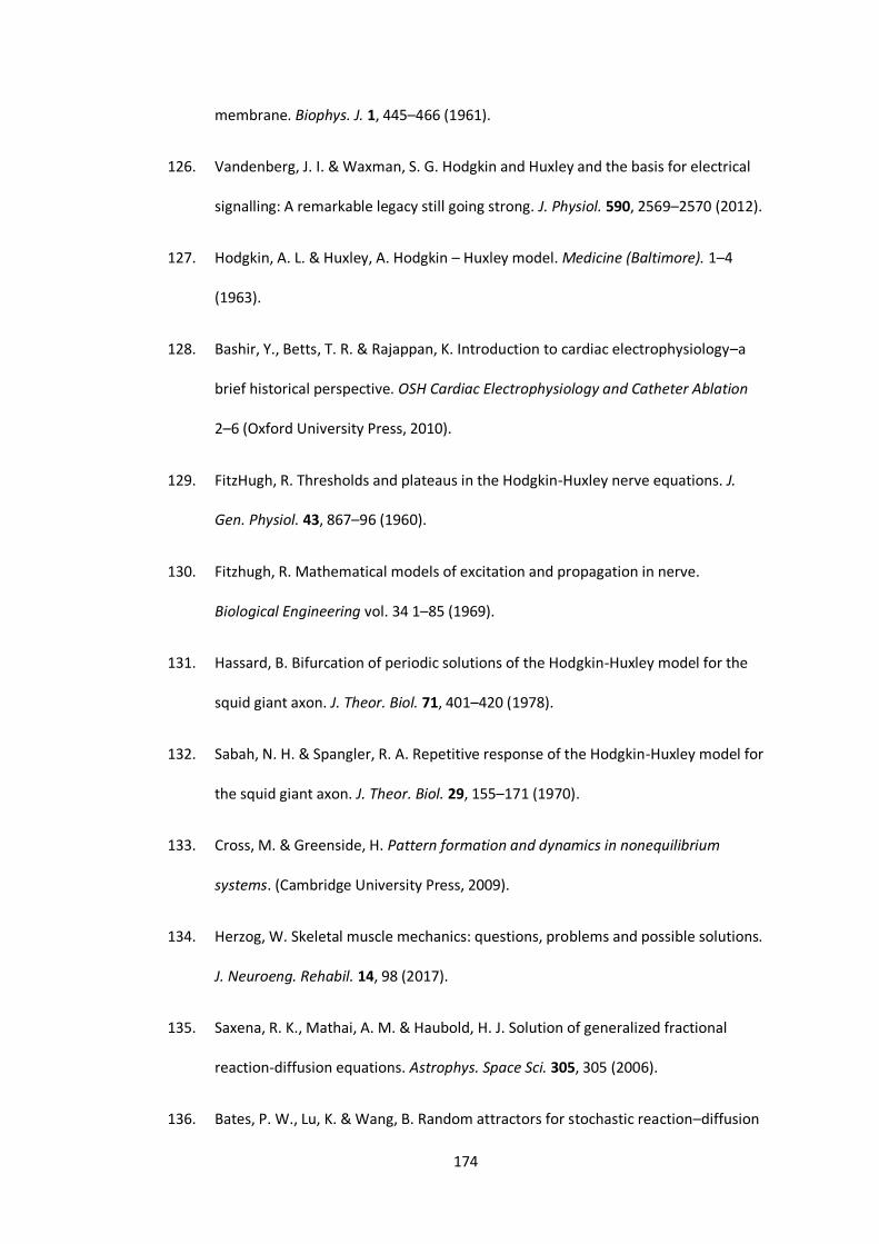
174
membrane. Biophys. J. 1, 445–466 (1961).
126. Vandenberg, J. I. & Waxman, S. G. Hodgkin and Huxley and the basis for electrical
signalling: A remarkable legacy still going strong. J. Physiol. 590, 2569–2570 (2012).
127. Hodgkin, A. L. & Huxley, A. Hodgkin – Huxley model. Medicine (Baltimore). 1–4
(1963).
128. Bashir, Y., Betts, T. R. & Rajappan, K. Introduction to cardiac electrophysiology–a
brief historical perspective. OSH Cardiac Electrophysiology and Catheter Ablation
2–6 (Oxford University Press, 2010).
129. FitzHugh, R. Thresholds and plateaus in the Hodgkin-Huxley nerve equations. J.
Gen. Physiol. 43, 867–96 (1960).
130. Fitzhugh, R. Mathematical models of excitation and propagation in nerve.
Biological Engineering vol. 34 1–85 (1969).
131. Hassard, B. Bifurcation of periodic solutions of the Hodgkin-Huxley model for the
squid giant axon. J. Theor. Biol. 71, 401–420 (1978).
132. Sabah, N. H. & Spangler, R. A. Repetitive response of the Hodgkin-Huxley model for
the squid giant axon. J. Theor. Biol. 29, 155–171 (1970).
133. Cross, M. & Greenside, H. Pattern formation and dynamics in nonequilibrium
systems. (Cambridge University Press, 2009).
134. Herzog, W. Skeletal muscle mechanics: questions, problems and possible solutions.
J. Neuroeng. Rehabil. 14, 98 (2017).
135. Saxena, R. K., Mathai, A. M. & Haubold, H. J. Solution of generalized fractional
reaction-diffusion equations. Astrophys. Space Sci. 305, 305 (2006).
136. Bates, P. W., Lu, K. & Wang, B. Random attractors for stochastic reaction–diffusion

175
equations on unbounded domains. J. Differ. Equ. 246, 845–869 (2009).
137. He, J.-H. Α review on some new recently developed nonlinear analytical
techniques. Int. J. Nonlinear Sci. Numer. Simul. 1, 51 (2000).
138. Ziegel, E., Press, W., Flannery, B., Teukolsky, S. & Vetterling, W. Numerical Recipes:
The Art of Scientific Computing. Technometrics vol. 29 (Cambridge University Press,
1987).
139. Xavier, J. de B., Picioreanu, C. & van Loosdrecht, M. C. M. A general description of
detachment for multidimensional modelling of biofilms. Biotechnol. Bioeng. 91,
651–669 (2005).
140. Allen, R. J. & Waclaw, B. Bacterial growth: a statistical physicist’s guide. Rep. Prog.
Phys. 82, 16601 (2019).
141. Kreft, J.-U., Picioreanu, C., van Loosdrecht, M. C. M. & Wimpenny, J. W. T.
Individual-based modelling of biofilms. Microbiology 147, 2897–2912 (2001).
142. Martinez-Corral, R., Liu, J., Prindle, A., Süel, G. M. & Garcia-Ojalvo, J. Metabolic
basis of brain-like electrical signalling in bacterial communities. Philos. Trans. R.
Soc. B Biol. Sci. 374, 20180382 (2019).
143. Mikami, T., Asally, M., Kano, T. & Ishiguro, A. A reaction-diffusion model for
simulating the oscillatory expansion of biofilms. in The 2019 Conference on
Artificial Life 218–219 (MIT Press, 2019).
144. Volfson, D., Cookson, S., Hasty, J. & Tsimring, L. S. Biomechanical ordering of dense
cell populations. Proc. Natl. Acad. Sci. 105, 15346–15351 (2008).
145. Martinez-Corral, R., Liu, J., Süel, G. M. & Garcia-Ojalvo, J. Bistable emergence of
oscillations in growing Bacillus subtilis biofilms. Proc. Natl. Acad. Sci. 115, E8333--

176
E8340 (2018).
146. Keener, J. & Sneyd, J. Calcium dynamics. Mathematical physiology: I: cellular
physiology 273–346 (Springer New York, 2010).
147. Gutiérrez, M. et al. A new improved and extended version of the multicell bacterial
simulator gro. ACS Synth. Biol. 6, 1496–1508 (2017).
148. Verkhratsky, A. & Parpura, V. History of Electrophysiology and the Patch Clamp.
Patch-Clamp Methods and Protocols (eds. Martina, M. & Taverna, S.) 1–19
(Springer New York, 2014).
149. Vagos, M. R. S. S. et al. Computational modeling of electrophysiology and
pharmacotherapy of atrial fibrillation: Recent advances and future challenges.
Front. Physiol. 9, 1–29 (2018).
150. Cao, Y. et al. Gating of the TrkH ion channel by its associated RCK protein TrkA.
Nature 496, 317–322 (2013).
151. Chen, G.-Q., Cul, C., MAyer, M. L. & Gouaux, E. Functional characterization of a
potassium-selective prokaryotic glutamate receptor. Nat. Biotechnol. 402, 817–821
(1999).
152. Beagle, S. D. & Lockless, S. W. Electrical signalling goes bacterial. Nature 527, 44–
45 (2015).
153. Filosa, J. A. et al. Local potassium signaling couples neuronal activity to
vasodilation in the brain. Nat. Neurosci. 9, 1397–1403 (2006).
154. Gerstner, W. & Kistler, W. M. Spiking neuron models. (Cambridge University Press,
2002).
155. Hodgkin, A. L. & Huxley, A. F. A quantitative description of membrane current and

177
its application to conduction and excitation in nerve. J. Physiol. 117, 500–544
(1952).
156. Glen, C. M., Kemp, M. L. & Voit, E. O. Agent-based modeling of morphogenetic
systems: Advantages and challenges. PLOS Comput. Biol. 15, e1006577 (2019).
157. Bora, Ş. & Emek, S. Agent-Based modeling and simulation of biological systems.
Modeling and Computer Simulation Ch. 3 (IntechOpen, 2019).
158. Ferrante, E., Turgut, A. E., Dorigo, M. & Huepe, C. Elasticity-based mechanism for
the collective motion of self-propelled particles with springlike interactions: a
model system for natural and artificial swarms. Phys. Rev. Lett. 111, 268302 (2013).
159. Weber, C. A., Bock, C. & Frey, E. Defect-mediated phase transitions in active soft
matter. Phys. Rev. Lett. 112, 168301 (2014).
160. Branda, S. S., González-Pastor, J. E., Ben-Yehuda, S., Losick, R. & Kolter, R. Fruiting
body formation by Bacillus subtilis. Proc. Natl. Acad. Sci. U. S. A. 98, 11621–6
(2001).
161. Mohammed, B. S., Fields, D. A., Mittendorfer, B., Coggan, A. R. & Klein, S. Are
peristaltic pumps as reliable as syringe pumps for metabolic research? assessment
of accuracy, precision, and metabolic kinetics. Metabolism. 53, 875–878 (2004).
162. Mirtich, B. & Canny, J. Impulse-based simulation of rigid bodies. in Proceedings of
the 1995 symposium on Interactive 3D graphics - SI3D ’95 181- (ACM Press, 1995).
163. Ericson, C. Real-time collision detection : Christer Ericson. (Elsevier : Morgan
Kaufmann, 2005).
164. Jafri, M. S. & Keizer, J. On the roles of Ca2+ diffusion, Ca2+ buffers, and the
endoplasmic reticulum in IP3-induced Ca2+ waves. Biophys. J. 69, 2139–2153

178
(1995).
165. Nagy‐Ungvarai, Z., Ungvarai, J., Müller, S. C. & Hess, B. The role of curvature and
pulse width for transition to unstable wave fronts in the Belousov–Zhabotinsky
reaction. J. Chem. Phys. 97, 1004–1009 (1992).
166. Herzog, W. Skeletal muscle mechanics: questions, problems and possible solutions.
J. Neuroeng. Rehabil. 14, 98 (2017).
167. Bers, D. M. Calcium and Cardiac Rhythms. Circ. Res. 90, 14–17 (2002).
168. Stewart, P. S. Diffusion in biofilms. Journal of Bacteriology vol. 185 1485–1491
(2003).
169. Klavins, E. A language for modeling and programming cooperative control systems.
in IEEE International Conference on Robotics and Automation, 2004. Proceedings.
ICRA ’04. 2004 vol. 4 3403–3410 Vol.4 (2004).
170. Toole, G. & Hurdal, M. K. Turing models of cortical folding on exponentially and
logistically growing domains. Comput. Math. with Appl. 66, 1627–1642 (2013).
171. Ramakrishnan, P., Maclean, M., MacGregor, S. J., Anderson, J. G. & Grant, M. H.
Cytotoxic responses to 405nm light exposure in mammalian and bacterial cells:
Involvement of reactive oxygen species. Toxicol. Vitr. 33, 54–62 (2016).
172. Maclean, M., Anderson, J. G., MacGregor, S. J., White, T. & Atreya, C. D. A new
proof of concept in bacterial reduction: antimicrobial action of violet-blue light
(405 nm) in Ex Vivo stored plasma. J. Blood Transfus. 2016, 1–11 (2016).
173. Dai, T., Vrahas, M. S., Murray, C. K. & Hamblin, M. R. Ultraviolet C irradiation: An
alternative antimicrobial approach to localized infections? Expert Rev. Anti. Infect.
Ther. 10, 185–195 (2012).

179
174. Peker, I., Akca, G., Sarikir, C., Toraman Alkurt, M. & Celik, I. Effectiveness of
alternative methods for toothbrush disinfection: An in vitro study. Sci. World J.
2014, 1–9 (2014).
175. Yuan, Y. et al. Photodynamic antimicrobial chemotherapy with the novel amino
acid-porphyrin conjugate 4I: In vitro and in vivo studies. PLoS One 12, e0176529
(2017).
176. Hamblin, M. R. et al. Helicobacter pylori. Society 49, 2822–2827 (2005).
177. MacLean, M., Murdoch, L. E., MacGregor, S. J. & Anderson, J. G. Sporicidal effects
of high-intensity 405 nm visible light on endospore-forming bacteria. Photochem.
Photobiol. 89, 120–126 (2013).
178. McKenzie, K. et al. The effects of 405 nm light on bacterial membrane integrity
determined by salt and bile tolerance assays, leakage of UV-absorbing material and
SYTOX green labelling. Microbiology 162, 1680–1688 (2016).
179. Chiaviello, A., Postiglione, I. & Palumbo, G. Targets and mechanisms of
photodynamic therapy in lung cancer cells: a brief overview. Cancers (Basel). 3,
1014–1041 (2011).
180. Pattison, D. I. & Davies, M. J. Actions of ultraviolet light on cellular structures.
Cancer: Cell Structures, Carcinogens and Genomic Instability. 131–157 (Birkhäuser
Basel, 2006).
181. Sharma, P. & Dubey, R. S. Drought induces oxidative stress and enhances the
activities of antioxidant enzymes in growing rice seedlings. Plant Growth Regul. 46,
209–221 (2005).
182. Meriga, B., Reddy, B. K., Rao, K. R., Reddy, L. A. & Kishor, P. B. K. Aluminium-
induced production of oxygen radicals, lipid peroxidation and DNA damage in

180
seedlings of rice (Oryza sativa). J. Plant Physiol. 161, 63–68 (2004).
183. Mittler, R. Oxidative stress, antioxidants and stress tolerance. Trends Plant Sci. 7,
405–410 (2002).
184. Huynh, T. T. et al. Glucose starvation-induced dispersal of pseudomonas
aeruginosa biofilms is camp and energy dependent. PLoS One 7, e42874 (2012).
185. Moghoofei, M. et al. Morphological and bactericidal effects of amikacin,
meropenem and imipenem on Pseudomonas aeruginosa. Jundishapur J. Microbiol.
8, (2015).
186. Aalen, O. O., Borgan, Ø. & Gjessing, H. K. Survival and Event History Analysis - A
Process Point of View. Springer (2008).
187. Kaplan, E. L. & Meier, P. Nonparametric estimation from incomplete observations.
J. Am. Stat. Assoc. 53, 457–481 (1958).
188. Barraclough, H., Simms, L. & Govindan, R. Biostatistics primer: What a clinician
ought to know: Hazard ratios. J. Thorac. Oncol. 6, 978–982 (2011).
189. Cook, R. J. & Lawless, J. F. Event history analysis. International Encyclopedia of the
Social & Behavioral Sciences (Elsevier, 2015).
190. Schlesinger, D. et al. Equivalence of cell survival data for radiation dose and
thermal dose in ablative treatments: analysis applied to essential tremor
thalamotomy by focused ultrasound and gamma knife. Int. J. Hyperth. 33, 401–410
(2017).
191. Liu, J. et al. Metabolic co-dependence gives rise to collective oscillations within
biofilms. Nature 523, 550–554 (2015).
192. Locke, J. C. W., Young, J. W., Fontes, M., Jimenez, M. J. H. & Elowitz, M. B.

181
Stochastic pulse regulation in bacterial stress response. Science (80-. ). 334, 366–
369 (2011).
193. Alon, U. An introduction to systems biology: Design principles of biological circuits.
Chapman Hall/CRC (2007).
194. Elasri, M. O. & Miller, R. V. Study of the response of a biofilm bacterial community
to UV radiation. 65, 2025–2031 (1999).
195. Stover, C. K. et al. Complete genome sequence of Pseudomonas aeruginosa PAO1,
an opportunistic pathogen. Nature 406, 959–64 (2000).
196. Gomelsky, M. & Hoff, W. D. Light helps bacteria make important lifestyle decisions.
Trends Microbiol. 19, 441–448 (2011).
197. Braatsch, S. & Klug, G. Blue light perception in bacteria. Photosynth. Res. 79, 45–57
(2004).
198. Conrad, K. S., Manahan, C. C. & Crane, B. R. Photochemistry of flavoprotein light
sensors. Nat. Chem. Biol. 10, 801–809 (2014).
199. Dai, T. et al. Blue light for infectious diseases: Propionibacterium acnes,
Helicobacter pylori, and beyond? Drug Resist. Updat. 15, 233–236 (2012).
200. Hecker, M., Pané-Farré, J. & Uwe, V. SigB-dependent general stress response in
Bacillus subtilis and related gram-positive bacteria. Annu. Rev. Microbiol. 61, 215–
236 (2007).
201. Ávila-Pérez, M., Hellingwerf, K. J. & Kort, R. Blue light activates the σB dependent
stress response of Bacillus subtilis via YtvA. J. Bacteriol. 188, 6411 LP-6414 (2006).
202. Mukherjee, S., Jemielita, M., Stergioula, V., Tikhonov, M. & Bassler, B. L.
Photosensing and quorum sensing are integrated to control Pseudomonas

182
aeruginosa collective behaviors. PLOS Biol. 17, e3000579 (2019).
203. Wu, L., McGrane, R. S. & Beattie, G. A. Light regulation of swarming motility in
Pseudomonas syringae integrates signaling pathways mediated by a
bacteriophytochrome and a LOV protein. MBio 4, 1–9 (2013).
204. Terauchi, K. & Ohmori, M. Blue light stimulates cyanobacterial motility via a cAMP
signal transduction system. Mol. Microbiol. 52, 303–309 (2004).
205. Chua, S. L. et al. C-di-GMP regulates Pseudomonas aeruginosa stress response to
tellurite during both planktonic and biofilm modes of growth. Sci. Rep. 5, 10052
(2015).
206. Bruni, G. N., Weekley, R. A., Dodd, B. J. T. & Kralj, J. M. Voltage-gated calcium flux
mediates Escherichia coli mechanosensation. Proc. Natl. Acad. Sci. 114, 9445–9450
(2017).
207. Huynh, T. T. et al. Glucose starvation-induced dispersal of pseudomonas
aeruginosa biofilms is camp and energy dependent. PLoS One 7, (2012).
208. Lin Chua, S. et al. Reduced intracellular c-di-GMP content increases expression of
quorum sensing-Regulated genes in Pseudomonas aeruginosa. Front. Cell. Infect.
Microbiol. 7, 451 (2017).
209. Strempel, N., Nusser, M., Neidig, A., Brenner-Weiss, G. & Overhage, J. The
oxidative stress agent hypochlorite stimulates c-di-GMP synthesis and biofilm
formation in Pseudomonas aeruginosa. Front. Microbiol. 8, 2311 (2017).
210. Huang, C.-J., Wang, Z.-C., Huang, H.-Y., Huang, H.-D. & Peng, H.-L. YjcC, a c-di-GMP
phosphodiesterase protein, regulates the oxidative stress response and virulence
of Klebsiella pneumoniae CG43. PLoS One 8, e66740–e66740 (2013).

183
211. Fernandez, N. L. & Waters, C. M. Cyclic di-GMP increases catalase production and
hydrogen peroxide tolerance in Vibrio cholerae. Appl. Environ. Microbiol. 85,
e01043-19 (2019).
212. Plyuta, V. A., Andreenko, J. V, Kuznetsov, A. E. & Khmel’, I. A. Formation of
Pseudomonas aeruginosa PAO1 biofilms in the presence of hydrogen peroxide. The
effect of the aiiA gene. Mol. Genet. Microbiol. Virol. 28, 141–146 (2013).
213. Irie, Y. & Parsek, M. LC/MS/MS-based quantitative assay for the secondary
messenger molecule, c-di-GMP. Methods Mol. Biol. 1149, 271–279 (2014).
214. Rybtke, M. T. et al. Fluorescence-based reporter for gauging cyclic di-GMP Levels in
Pseudomonas aeruginosa. Appl. Environ. Microbiol. 78, 5060–5069 (2012).
215. Sinkeldam, R. W., Greco, N. J. & Tor, Y. Fluorescent analogs of biomolecular
building blocks: Design, properties, and applications. Chem. Rev. 110, 2579–2619
(2010).
216. Barbier, M. & Damron, F. H. Rainbow vectors for broad-range bacterial
fluorescence labeling. PLoS One 11, e0146827 (2016).
217. Koch, B., Jensen, L. E. & Nybroe, O. A panel of Tn7-based vectors for insertion of
the gfp marker gene or for delivery of cloned DNA into Gram-negative bacteria at a
neutral chromosomal site. J. Microbiol. Methods 45, 187–195 (2001).
218. Clark, D. J. & Maaløe, O. DNA replication and the division cycle in Escherichia coli. J.
Mol. Biol. 23, 99–112 (1967).
219. Choi, K.-H., Kumar, A. & Schweizer, H. P. A 10-min method for preparation of highly
electrocompetent Pseudomonas aeruginosa cells: Application for DNA fragment
transfer between chromosomes and plasmid transformation. J. Microbiol. Methods
64, 391–397 (2006).

184
220. Chua, S. L. et al. Reactive oxygen species drive evolution of pro-biofilm variants in
pathogens by modulating cyclic-di-GMP levels. Open Biol. 6, 160162 (2016).
221. Rodesney, C. A. et al. Mechanosensing of shear by Pseudomonas aeruginosa leads
to increased levels of the cyclic-di-GMP signal initiating biofilm development. Proc.
Natl. Acad. Sci. 114, 5906–5911 (2017).
222. Ganini, D. et al. Fluorescent proteins such as eGFP lead to catalytic oxidative stress
in cells. Redox Biol. 12, 462–468 (2017).
223. Piatkevich, K. D. & Verkhusha, V. V. Guide to red fluorescent proteins and
biosensors for flow cytometry. Methods Cell Biol. 102, 431–461 (2011).
224. Dixit, R. & Cyr, R. Cell damage and reactive oxygen species production induced by
fluorescence microscopy: effect on mitosis and guidelines for non-invasive
fluorescence microscopy. Plant J. 36, 280–290 (2003).
225. Różanowska, M. et al. Blue light-induced singlet oxygen generation by retinal
lipofuscin in non-polar media. Free Radic. Biol. Med. 24, 1107–1112 (1998).
226. Bjarnsholt, T. et al. Pseudomonas aeruginosa tolerance to tobramycin, hydrogen
peroxide and polymorphonuclear leukocytes is quorum-sensing dependent.
Microbiology 151, 373–383 (2005).
227. Elkins, J. G., Hassett, D. J., Stewart, P. S., Schweizer, H. P. & McDermott, T. R.
Protective role of catalase in Pseudomonas aeruginosa biofilm resistance to
hydrogen peroxide. Appl. Environ. Microbiol. 65, 4594–4600 (1999).
228. Bond, D. R. & Lovley, D. R. Electricity production by Geobacter sulfurreducens
attached to electrodes. Appl. Environ. Microbiol. 69, 1548–1555 (2003).
229. Schlafer, S. & Meyer, R. L. Confocal microscopy imaging of the biofilm matrix. J.

185
Microbiol. Methods 138, 50–59 (2017).
230. Murdoch, L. E., Maclean, M., Endarko, E., MacGregor, S. J. & Anderson, J. G.
Bactericidal effects of 405 nm light exposure demonstrated by inactivation of
Escherichia, Salmonella, Shigella, Listeria, and Mycobacterium species in liquid
suspensions and on exposed surfaces. Sci. World J. 2012, 1–8 (2012).
231. Kalyanaraman, B. et al. Measuring reactive oxygen and nitrogen species with
fluorescent probes: challenges and limitations. Free Radic. Biol. Med. 52, 1–6
(2012).
232. Renggli, S., Keck, W., Jenal, U. & Ritz, D. Role of autofluorescence in flow
cytometric analysis of escherichia coli treated with bactericidal antibiotics. J.
Bacteriol. 195, 4067–4073 (2013).
233. McBee, M. E. et al. Production of superoxide in bacteria is stress- and cell state-
dependent: A gating-optimized flow cytometry method that minimizes ROS
measurement artifacts with fluorescent dyes. Front. Microbiol. 8, 459 (2017).
234. Liu, Y. & Imlay, J. A. Cell death from antibiotics without the involvement of reactive
oxygen species. Science (80-. ). 339, 1210–1213 (2013).
235. Oparka, M. et al. Quantifying ROS levels using CM-H2DCFDA and HyPer. Methods
109, 3–11 (2016).
236. Seistrup, K. H., Strahl, H., Hamoen, L. W., Gray, D. A. & te Winkel, J. D. Analysis of
antimicrobial-triggered membrane depolarization using voltage sensitive dyes.
Front. Cell Dev. Biol. 4, 1–10 (2016).
237. Masson-Meyers, D., Bumah, V., Biener, G., Raicu, V. & Enwemeka, C. The relative
antimicrobial effect of blue 405 nm LED and blue 405 nm laser on methicillin-
resistant Staphylococcus aureus in vitro. Lasers Med. Sci. 30, (2015).

186
238. Ganini, D. et al. Fluorescent proteins such as eGFP lead to catalytic oxidative stress
in cells. Redox Biol. 12, 462–468 (2017).
239. Becker, W. Fluorescence lifetime imaging - techniques and applications. J. Microsc.
247, 119–136 (2012).