INVESTIGATION OF MIXING IN A

MULTISTAGE AXIAL COMPRESSOR

by

Sasi K. DigavalliB.Tech., Indian Institute of Technology, (1986)

SUMMITED IN PARTIAL FULFILLMENT

OF THE REQUIREMENTS FOR THE DEGREE OF

MASTER OF SCIENCE

IN AERONAUTICS AND ASTRONAUTICS

at the

MASSACHUSETTS INSTITUTE OF TECHNOLOGY

May1990

@ Massachusetts Institute of Technology

Signature of Author _Department of Aeronautics and Astronautics, May, 1990

Certified byProfessor Edward M. Greitzer

Thesis SupervisorDepartment of Aeronautics and Astronautics

Accepted byProfe sor Harold Y. Wachman

Chairman, Department Graduate Committee

INVESTIGATION OF MIXING IN AMULTISTAGE AXIAL COMPRESSOR

bySasi K. Digavalli

The work described in this thesis consists of an experimentalinvestigation of mixing in a three stage axial compressor, in particular itsevolution through the machine. A tracer gas is used to measure the mixingrates. The variation in mixing rates with position in the machine is examined.The effects of injection probe geometry and external flow parameters on theresults are also investigated.

It is found that mixing across all three stators is very similar, as it isacross all three rotors and across all three stages. There is little evidence ofany evolution of the mixing process. Radial and circumferential flow distortionsgenerated in one blade row do not affect mixing in the next blade row toany significant degree. Secondary flows contribute to mixing only near the endwalls. At increased loading there is increased mixing in both stators and inrotors.

Thesis Supervisor : Dr. Edward M. GreitzerTitle : Professor of

Aeronautics and Astronautics

ACKNOWLEDGEMENTS

The completion of this thesis would not have been possible without the

advice, help and encouragement of many people at the GTL

First, I would like to express my respect and appreciation to Prof. E M.

Greitzer for his supervision and encouragement His constant emphasis on data

interpretation rather than on data taking has greatly broadened my vision of

experimental investigation and understanding of fluid mechanics. Dr. C. S. Tan's

criticism and advice have been very constructive and helpful.

Mr. Victor Dubrowski's patient and immaculate work during restaggering

the low speed compressor and in the machine-shop will never be forgotten.Mr. Jim Nash and Mr. Roy Andrew have been very helpful in setting up the rigfor running the compressor and moving around gas cylinders. Mr. Dave Dvore'swork in replacing the computer system in the laboratory was very efficientand made the computer more user friendly.

A wealth of software left behind by Dr. P. L Lavrich and Dr. David Finkhas saved me a lot of time. The comraderie and cheering-up of Mr. TonghuoShang have made the long working hours look much shorter.

Financial support for the work was provided by Pratt and WhitneyAircraft Government Products Division and it is greatly appreciated Theinterest and helpful comments of Dr. S. Baghdadi and Dr. S. Koff are verymuch appreciated

I am also thankful to the U.S. Government for giving me the opportunityto study in this country.

Finally the work would have been impossible without the constantencouragement of my parents, sister and brother.

ABSTRACTACKNOWLEDGEMENTSTABLE OF CONTENTSLIST OF TABLESLIST OF FIGURES

CHAPTER 1INTRODUCTION ........................................ . 1

1.A Introduction .................................. 11.B Background .................................... 21.C Thesis Objectives ............................. 41.D Scope of the Thesis ........................... 5

CHAPTER 2TRACER GAS TECHNIQUE .................................... 6

2.A Description of the Technique .................. 62.B Flame Ionization Detector ..................... 7

CHAPTER 3MIXING COEFFICIENT ..................................... 10

3.A Introduction ................................. 103.B Methods for Predicting Mixing Coefficient .... 103.C Influence of Probe and Flow Parameters on

Mixing ....................................... 13

CHAPTER 4INSTRUMENTATION ANDEXPERIMENTAL TECHNIQUES ................................ 20

4.A Compressor and Rig Description ............... 204.B Data Acquisition System ...................... 204.C Experimental Techniques ...................... 234.D Compressor Performance ....................... 25

CHAPTER 5TRACER GAS EXPERIMENT .................................. 27

5.A Ethylene Injection and Sampling .............. 275.B Data Reduction Procedure ......................305.C Results of Ethylene Tracing Measurements ...... 30

CHAPTER 6CONCLUSIONS AND SUGGESTIONS ............................ 36

6.A Conclusions .................................. 366.B Suggestions for Future Research .............. 38

TABLES

FIGURES

REFERENCES

IJST OF TABLES

Table 1 Compressor Design Specifications.

Table 2 Compressor Blading Design.

Table 3 Summary of Available Mixing Coefficient Data.

LIST OF FIGURES

Fig. Tracer Gas Detection System.

Fig. 2 Flame Ionization Detector.

Fig. 3 FID Response to Sample Flow Rate Variations.

Fig.

Fig.

FID Response to Hydrogen Flow Rate Variations

FID Response to Air Flow Rate Variations.

Fig. 6 Linearity of FID Signal.

Fig. 7 Effects of a Heated Sample-line on FID Output

Fig. 8 Schematic of Injection from a Jet into a Uniform Stream.

Fig. 9 Streamwise Variation of Turbulence Intensityin a Wind-tunnel Fitted with Screens.

Fig 10 Highest Turbulence Level Achieved in Wind-tunnel.

Fig. 11 Profile of Nonuniform Turbulence Intensity.

Fig. 12 Test of Symmetry of the 1" Round Jet

Fig. 13 Velocity Profile of the Jet

Fig. 14 Turbulence Intensity in the Jet

Fig. 15 Length Scales in Similarity Region of the Jet

Fig. 16 Effect of Injection Probe Diameteron Tracer Gas Spreading.

Fig. 17 Effect of Injection Probe Lengthon Tracer Gas Spreading.

Fig. 18 Effect of Turbulence on Tracer GasSpreading; Case-I : Potential Flow

Fig. 19 Effect of Turbulence on Tracer GasSpreading; Case-l : 10% Turbulence

Fig. 20 Effect of TurbulenceSpreading; Case-Ill :

Fig. 21 Effect of TurbulenceSpreading; Case-IV :

on Tracer Gas18% Turbulence

on Tracer Gas25% Turbulence

Fig. 22 Variation of Mixing Coefficient withTurbulence LeveL

Fig. 23 Variation of Mixing Coefficient withMain Stream Velocity.

Fig. 24 Low Speed Compressor Rig Schematic.

Fig. 25 Steady-state Measurement Locations.

Fig. 26 Total to Static Pressure Performance.

Fig. 27 Stator Exit Flow Angles atDesign Point Loading.

Fig. 28 Stator Exit Flow Angles atIncreased Loading.

Fig. 29 Radial Variation of Turbulence LevelsUpstream of 1st. Stator.

Fig. 30 Radial Variation of Turbulence LevelsUpstream of 2nd. Stator.

Fig. 31 Radial Variation of Turbulence LevelsUpstream of 3rd. Stator.

Fig. 32 Contour Plots for Tracer Gas Spreading

Across 1st Stator at Design Point Loading.

Fig. 33 Contour Plots for Tracer Gas SpreadingAcross lst. Stator at Increased Loading.

Fig. 34 Contour Plots for Tracer Gas SpreadingAcross 1st Rotor at Design Point Loading.

Fig. 35 Contour Plots for Tracer Gas SpreadingAcross lst Rotor at Increased Loading.

Fig. 36 Contour Plots for Tracer Gas SpreadingAcross 2nd. Stator at Design Point Loading.

Fig. 37 Contour Plots for Tracer Gas SpreadingAcross 2nd. Stator at Increased Loading.

Fig. 38 Contour Plots for Tracer Gas SpreadingAcross 2nd. Rotor at Design Point Loading.

Fig. 39 Contour Plots for Tracer Gas SpreadingAcross 2nd. Rotor at Increased Loading.

Fig. 40 Contour Plots for Tracer Gas SpreadingAcross 3rd. Stator at Design Point Loading.

Fig. 41 Contour Plots for Tracer Gas SpreadingAcross 3rd. Stator at Increased Loading.

Fig. 42 Contour Plots for Tracer Gas SpreadingAcross 3rd. Rotor at Design Point Loading.

Fig. 43 Contour Plots for Tracer Gas SpreadingAcross 3rd. Rotor at Increased Loading.

Fig. 44 Contour Plots for Tracer Gas SpreadingAcross IGV at Design Point Loading.

Fig. 45 Contour Plots for Tracer Gas SpreadingAcross IGV at Increased Loading.

Fig. 46 Contour Plots for Tracer Gas SpreadingAcross 1st. stage at Design Point Loading.

Fig. 47 Contour Plots for Tracer Gas SpreadingAcross lst. Stage at Increased Loading.

Fig. 48 Contour Plots for Tracer Gas SpreadingAcross 2nd. stage at Design Point Loading.

Fig. 49 Contour Plots for Tracer Gas SpreadingAcross 2nd. Stage at Increased Loading.

Fig 50 Contour Plots for Tracer Gas SpreadingAcross 3rd. stage at Design Point Loading.

Fig. 51 Contour Plots for Tracer Gas SpreadingAcross 3rd. Stage at Increased Loading.

Fig. 52 Radial Distribution of Mixing Coefficientfor 1st. Stator.

Fig. 53 Radial Distributionfor 2nd. Stator.

Fig. 54 Radial Distributionfor 3rd. Stator.

Fig. 55 Radial Distributionfor 1st. Rotor.

Fig. 56 Radial Distributionfor 2nd. Rotor.

Fig. 57 Radial Distributionfor 3rd. Rotor.

Fig. 58 Radial Distributionfor IGV.

Fig. 59 Radial Distributionfor 1st. Stage

Fig. 60 Radial Distributionfor 2nd. Stage.

Fig. 61 Radial Distributionfor 3rd. Stage

of Mixing Coefficient

of Mixing Coefficient

of Mixing Coefficient

of Mixing Coefficient

of Mixing Coefficient

of Mixing Coefficient

of Mixing Coefficient

of Mixing Coefficient

of Mixing Coefficient

Fig. 62 Evolution of Mixing Through the Compressor.

CHAPTER 1

INTRODUCTION

1 A INTRODUCTION

With the present trend in axial flow compressor design towards low

aspect ratio, a greater fraction of the annulus flow is subjected to end-wall

effects. Although one might expect the losses at the end-walls to produce

increasing temperature and velocity defects in this vicinity as the flow

progresses through the machine, this phenomenon in fact does not occur after

the first one or two stages [Ref. 11 Measurements of flows in multi-stage

compressors show the existence of a repeating stage condition, where the

velocity profiles upstream and downstream of a stage are almost identical.

Such a repeating stage condition indicates the existence of a radial mixing

mechanism which causes the end-wall losses to be mixed out towards the mid-span

and prevents steepening of velocity profiles. Measurements [Ref. 2] indicating

higher efficiency near end-walls than those predicted have lent further evidence

to the hypothesis that radial mixing plays an important role in flow through

multi-stage axial compressors.

This thesis examines the mechanisms that cause the mixing, their

relative importance and the variation of mixing rates as flow progresses

through a multi-stage axial compressor.

1 BACKGROUND

Considerable research has gone into understanding the mechanisms of

fluid migration and radial mixing in a multi-stage compressor and a brief

outline of these developments is given below.

Based on the higher measured efficiencies at tip than predicted by

through-flow calculations and the idea that this was due to radial mixing,

Adkins and Smith [Ref. 2] postulated that the mechanism driving radial

redistribution was a large scale secondary flow. They devised a method of

including this effect in a through-flow calculation. Their model used inviscid,

small-perturbation secondary flow theory to obtain radial velocities, which

were used to calculate spanwise mixing coefficient Flow properties were then

redistributed radially by solving an equation which models a diffusion process.

Inclusion of their spanwise mixing model in compressor through-flow calculations

led to computed results that were in good agreement with radial profiles of

total temperature observed during compressor tests.

Gallimore and Cumpsty [Ref. 3] examined this concept using a tracer

gas technique. They measured mixing in two multi-stage compressors and concluded

that the convective model of [Ref. 2] did not include the main source of

the mixing, because the dominant mixing mechanism was a "turbulent diffusion"

process. They found that the levels of mixing were high all the way across

the span, and that the idea of separate end-wall boundary layers bounding a

free stream is not appropriate. Local spanwise mixing coefficients were derived

by assuming that the tracer gas diffuses from a point source into uniform

flow. Like Adkins and Smith [Ref. 2] they used their mixing coefficients in a

through-flow calculation to obtain radial profiles of flow properties in a

compressor. Their predicted spanwise distributions of total temperature also

agree with experimental results, particularly away from end-walls.

It is reasonable to state, based on the results reported in [Ref. 2,3]

that regardless of the underlying mechanism, inclusion of a mixing coefficient

into through-flow calculation of an axial compressor improves the predicted

results. A relevant comment is that made by Wennerstrom [Ref. 41 It is,however, it

important to understand the mechanisms that contribute to radial mixing, and

further insight into this problem has been provided by Wisler et al [Ref. 51

They investigated the relative importance of convection by secondary flows and

diffusion by turbulence as mechanisms responsible for spanwise mixing in the

third-stage of a four stage axial compressor. They concluded that away from

the end-walls diffusion is the dominant mechanism, whereas close to the

end-walls contributions to mixing from secondary flows and turbulence are of

the same magnitude.

Li and Cumpsty [Ref. 6] have investigated mixing across several

stages of a multistage compressor. Their measurements indicate that the

level of mixing does not change appreciably from one stage to the next

They also stated that contribution to mixing by secondary flows is appreciable

only close to the end walls.

Though the mixing levels predicted by [Ref. 2,3] agree with experi-

ments, they are based on two fundamentally different mechanisms and more data

is needed before one can lend support to either of these hypotheses. A brief

outline of the focus of the present research, the motivation, and the main

findings of the investigation is given in the next section.

1.C RESEARCH OBJECTIVES

As stated earlier a complete understanding of all the mechanisms that

generate radial mixing is far from complete. The consensus seems to be that

turbulent diffusion dominates the mixing process through most of the span away

from the end-walls and that contributions from secondary radial flows are

significant only near end-walls. One of the objectives of this thesis is to

clarify the relative importance of secondary flows and turbulent diffusion for

radial mixing.

The results that have been reported so far, except for Li and

Cumpsty [Ref. 6], are confined to radial mixing across a single blade row,

in each case. Wisler et al [ Ref. 5] studied extensively the third stator in

a four stage compressor, but no other blade row. Adkins and Smith [Ref. 2]

applied their theory mostly to a single blade row in each machine they picked

for demonstration. Gallimore and Cumpsty [Ref. 3] measured mixing coefficients

for a stator, in each of the two compressors they studied. An additional

question is how the mixing level evolves through the compressor. Another goal

of this thesis, therefore, is to carry out detailed mixing measurements for

each blade row in a multi-stage compressor to understand how the mixing process

evolves, as flow passes through the compressor. (Results from Ref. 6 were not

available when this research effort began.)

It is also intended that the effect of Aspect Ratio on mixing be

defined. As Aspect Ratio is decreased, secondary flows will increase in

significance, the assumption of parallel stream tubes will be less valid and

consequently mixing should increase. Mixing measurements will be available from

four compressors ( two from [Ref. 3], the third from [Ref. 5] ), so a

comparative study between mixing levels and Aspect Ratio will be possible.

Finally, Gallimore and Cumptsy [Ref. 3] used different kinds of probes

for injecting the tracer gas. There are effects of probe shape and relative

size on mixing of the injected fluid with external flow. We have thus documented

the effects of external flow velocity and turbulence on mixing of an injected

fluid with the external flow.

1D SCOPE OF THE THESIS

The following chapter describes the principle of the tracer gas

technique, used in the mixing measurements. A brief account of the operation

of a Flame Ionization Detector which is a fundamental part of the tracer gas

experiments is also included. Chapter 3 details methods for estimating mixing

coefficients by using results from tracer gas experiments. Effects of external

flow parameters and injection probe geometry on mixing coefficient are also

discussed. Chapter 4 discusses the instrumentation and the experimental

techniques used in this work. Chapter 5 describes a detailed experiment carried

out to study mixing in a three-stage axial compressor. Chapter 6 presents

conclusions and suggestions for further research.

CHAPTER 2

TRACER GAS TECHNIQUE

2.A DESCRIPTION OF THE TECHNQUE

The principal idea behind the tracer gas technique is similar to that

behind flow visualization methods. A tracer gas is injected into the stream

of air that is being studied. As the tracer gas is carried downstream by the

main stream it is detected either by direct visualization, as is the case if

the tracer gas is smoke, or by measuring some property of the fluid (e.g.

concentration or conductivity), which is affected by the presence of the tracer

gas. For example, Kerrebrock and Mikolajczak [Ref. 7] used helium and a

conductivity probe to study the migration of rotor wakes inside a stator row.

The method that we used to investigate the flow in a multi-stage

compressor was first adopted to mixing analysis by Denton and Usui [Ref. 81

Ethylene was chosen as the tracer gas since it has almost the same density as

air. A small steady stream of ethylene is injected into the main flow from an

injection probe, with the flow rate monitored by a flowmeter. The air, mixed

with ethylene, is then sampled downstream at a constant rate using a sampling

probe connected to a Flame Ionization Detector (FID). The voltage output of

the FID is then converted to concentration in parts per million of ethylene.

These concentration measurements can be used to obtain mixing rates.

2. FLAME IOMZATION DETECTOR (FID)

The concentration of tracer gas is measured using a commercially

available FID. The FID employs a hydrogen flame in air to detect the presence

of ions produced by combusting the hydrocarbons present in the sample. It has

high sensitivity, being able to detect mass flow rates of ethylene as low as

10-10 gm/s, or concentrations of a few ppm. The FID used was Beckman

Industrials model #400A. The gas detector system is comprised of the following

components connected as shown in Fig. 1.

1. FID

2. Tracer gas injection probe

3. Sampling probe

4. Suction pump

5. Flowmeters

6. Flow control valves

7. Hydrogen, Ethylene and Air cylinders.

Fig. 2 shows a diagram of the FID combustion chamber.

As shown in Fig. 1, air containing a small quantity of tracer gas, is

sucked into a sampling probe inserted into the flow being studied. After

passing through a flowmeter and a valve the sample is mixed with a stream

of hydrogen. This gas mixture enters the flame chamber of the FID. When ignited,

the hydrogen burns and maintains a steady flame. Within the flame, the

hydrocarbon components of the sample stream undergo an ionization process

that produces electrons and positive ions. Polarized electrodes collect these

ions, causing current to flow through an electronic measuring circuitry. The

burner jet and the collector function as electrodes. Current flow is proportional

to the rate at which carbon atoms enter the burner. The ionization current is

amplified twice, first by a preamplifier and then by a post-amplifier after

passing through a filter.

It is important that the flow rates of all the gases going into the

FID be kept constant during the experiment since the response of the FID

varies with all these flow rates. Their relative values should be chosen so

that peak response and maximum flame stability are achieved. In addition, the

hydrogen used for flame generation was mixed with helium (40%) to prevent

burner overheating. In the experiments (chapter 3&5) the sample flow rate was

matched with local external velocity. The time taken by the FID to reach a

steady output and the flame stability depend on the sample flow rate. When

the sample flow rate was too high for the flame to be stable a by-pass was

used.

Fig. 3,4 and 5 show how FID response (output measured in volts)

varies when input pressures of sample, fuel and air flow were varied,

respectively. Fig. 6 shows the linearity between FID output and the

concentration of sample when ethylene samples of known concentrations were

used.

Some FID models, used mainly in automobile exhaust studies, are fitted

with heated sample-lines to prevent condensation of heavy hydrocarbons on the

9

walls of the tubing. To find out whether a heated line was necessary when the

sample is ethylene, an experiment was conducted using a heated FID. The FID

was fed with an ethylene sample of known concentration and its output was

measured, once with sample-line heat switched off and another time with

the heat on. A comparison of these two measurements is shown in Fig. 7. The

difference between these two readings was within the margin of accuracy of

the machine, so it was concluded that for ethylene a heated line was

unnecessary.

CHAPTER S

ESTIMATION OF MIXING COEICIENTS

3.A INTRODUCTION

It was mentioned in chapter 1 that mixing rates will be determined

from the tracer gas concentration measurements taken on the multi-stage

compressor (presented in chapter 5). If the mechanism is turbulent diffusion,

these mixing rates imply eddy mixing coefficients, and analyses are presented

in the next section for estimating these eddy diffusion coefficients from

the concentration measurements. One of these analyses, originally developed by

Towle and Sherwood [Ref. 9] has been used by Gallimore and Cumpsty [Ref. 31

In this approach the injector is modelled as a point source. Another approach

described here, is a simplified version of a method given in Hinze [Ref. 10]

where the injection source is modelled as a jet The author views the latter

as a better approximation because the representation of the injection source

is closer to the actual situation. In addition to these calculations,

experiments to determine the influence of injection probe and external flow

parameters on eddy diffusivity will be descussed.

3.B METHODS FOR PREDICTING THE MIXING COEFFICIENT

i) MODEL#1 : Point Source Model:-

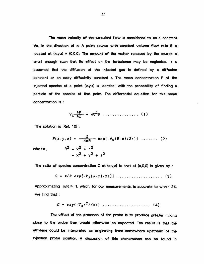
The mean velocity of the turbulent flow is considered to be a constant

Vx, in the direction of x. A point source with constant volume flow rate S is

located at (x,yz) - (0,0,0). The amount of the matter released by the source is

small enough such that its effect on the turbulence may be neglected. It is

assumed that the diffusion of the injected gas is defined by a diffusion

constant or an eddy diffusivity constant e. The mean concentration P of the

injected species at a point (x,y,z) is identical with the probability of finding a

particle of the species at that point The differential equation for this mean

concentration is :

Vx- - ev2p .............. (1)ex

The solution is [Ref. 10]:

P(x,y,z) = 4rR exp{-Vx(R-x)/2e)} ....... (2)

where, R2 -x 2 + r2

- x 2 + y 2 + ,2

The ratio of species concentration C at (x,yz) to that at (x,0,0) is given by :

C - x/R expf-Vx(R-x)/2e)) ................... (3)

Approximating x/R -= 1, which, for our measurements, is accurate to within 2%,

we find that :

C - expf-Vxr 2/4xe) .................... (4)

The effect of the presence of the probe is to produce greater mixing

close to the probe than would otherwise be expected. The result is that the

ethylene could be interpreted as originating from somewhere upstream of the

injection probe position. A discussion of this phenomenon can be found in

Moore and Smith [Ref. 11], who proposed a correction for the position of the

imaginary source position by introducing an empirical constant xO. Thus

C - expf-Vxr2/4(x-xo)e} .................... (5)

This constant depends on the probe geometry, and a of a method for determining

it is included in the next chapter.

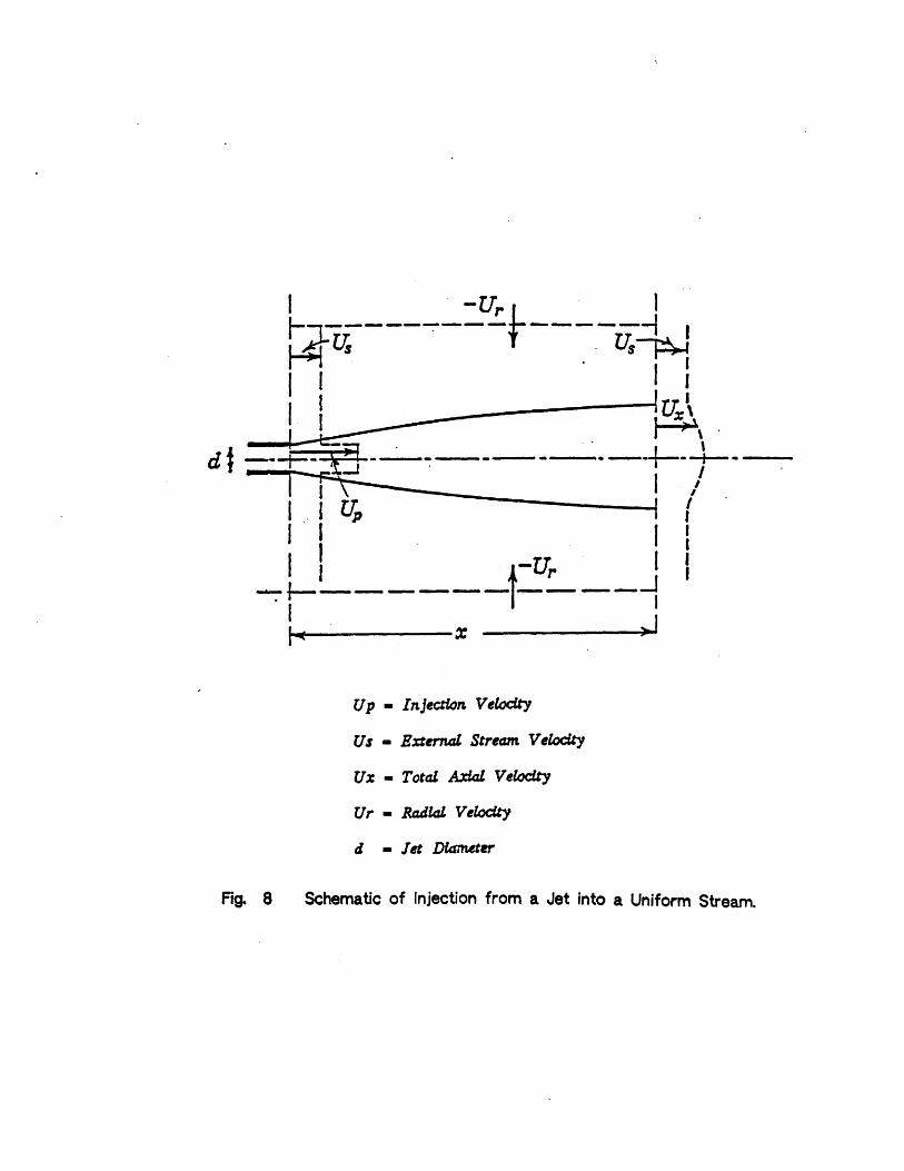
ii) MODEL#2 : Free Jet Model :-

This approach models the mixing coefficient for a species injected in

the form of a round free jet into a general turbulent stream of constant

velocity. Fig. 8 shows the general case of injection and the notation followed.

The outside turbulent stream has a velocity Us. The jet issues with a velocity

Up and concentration Cp from an orifice of diameter 'd'. Cylindrical

coordinates (x,r) are used with the axial coordinate 'x' along the jet axis,

and x-0 is the plane of the orifice.

The equation for transport of species concentration, after applying the

approximations associated with free turbulence [Ref. 101 is:

1 + Or 8C 1( re ) ....... (6)ax o r r (r ar

Similarity methods discussed by Abramovich [Ref. 12] provide the

solution of equation (6). For region U1/Up"<1, Ur/Up(<l and r/x <( 1

the solution simplifies to :

C - expf-Ur 2 6(x+a)e) .................... (7)

where C is the ratio of concentration at (x,r) to that at (x,O) and a is the

distance between the geometrical origin of similarity and the origin of the

coordinate system. We will take 'a' to be the same as the negative of 'x0' of model

#1. Its value is evaluated in the next chapter.

3.C INFLUENCE OF PROBE AND FLOW PARAMETERS ON MIXING

It was stated earlier that understanding of the factors influencing

the level of mixing in a tracer gas experiment is important Because of this,

investigations were carried out to define the effects of : size and shape of

the injection probe, turbulence level of the main stream, difference in speed

between main stream and injected gas, and streamwise large eddy length scale

of the main stream. To calibrate the mixing coefficient against these parameters

a uniform flow of known turbulence and length scales was needed. A preliminary

experiment on a wind tunnel was conducted to test suitability for this purpose.

Using square meshes, flows of different turbulence levels were gene-

rated. The largest length scales in the flow field are determined by the

spacing between the rods of the grid in use. Experiments were conducted with

meshes of 1" and 1/2" spacing and rod diameters ranging from 1/12" to 1/2".

Fig. 9 shows that at about 30 diameters downstream into the wake of the grid

the flow attains a uniform turbulence level, in accordance with with results

obtained in [Ref. 131 The maximum turbulence, however, was less than 5%, as

shown in Fig.10, which corresponds to a mesh of solidity 0.5 and rod diameter

1/2". Typical turbulence levels in axial compressors are roughly 7-10%, [Ref.

141 Meshes with larger rod diameter, needed for higher turbulence levels,

give a uniform turbulence only farther downstream. As an example Fig. 11 shows

the nonuniform turbulence field measured at 20 rod diameters downstream of a

screen. Meshes with larger rods could not be used due to lack of test section

space. In addition, increasing solidity beyond 0.5 can lead to jet coaliscence

instability as discussed in [Ref. 131 Thus we did not pursue the wind tunnel

calibration experiments further.

Several other schemes [Ref. 15,16] were then considered and it was

found that free (round) jet give a wide range of turbulence levels from zero,

in the potential core, to about 25% in the self-preserving region. In that

region the turbulence level remains constant for roughly 10 diameters so that

this configuration is useful to provide the external flow for the calibration

experiment

The calibration experiments were carried out using a 1" diameter free

jet. Hot wires were used for all velocity measurements. Before starting the

investigation on ethylene spreading several tests were run to ensure that the

flow issuing from the jet confirmed to measurements documented in the literature

[Ref. 12,171. Fig. 12 shows measurements of the jet velocity profiles at several

axial locations. Fig. 13 shows the variation of jet centerline velocity as a

function of distance from the orifice and fig. 14 gives the turbulence level

on the centerline of the jet. Turbulence intensities along lines that make

constant angles with the jet axis also are shown in Fig. 14. All these

measurements are consistent with those reported in the literature cited.

The integral length scale X in a turbulent flow with an average velocity

U and a fluctuating component of u' is given by :

00

X - U ff(' ) d' ................... (8)0

where the function f(r) is the autocorrelation at time r given by :

u'(t)u'(t+,r) (9)u' (t)u' (t)

Autocorrelations were measured at four locations on the axis of the jet at

x/d - 25, 29, 33, 37. Fig. 15 shows f(r) as a function of r at x/d - 25.

The same figure also includes the integral length scale X as a function of

distance from the jet orifice. In the region investigated the length scale

changes only by less than 10% (from 5cm. to 5.5cm).

Probes for injecting and sampling ethylene were made from high strength

steel tubing of several different diameters. The tube was heated and bent 90

degrees to give an 'L' shaped probe. Care was taken to ensure that a proper

radius was given at the bend to avoid excessive contortion of the passage.

According to [Ref. 3] 'L' shaped probes were as good as any other probes they

tested so that other shapes were not investigated.

Ethylene was injected into the jet along its centerline through probes

of different diameters and streamwise arm lengths. The ethylene was sampled 2"

downstream (typical rotor and stator chords in the multi-stage compressor are

roughly 2 and 1.2 inches). The sample was fed into a flame ionization detector

(FID), and concentration curves were plotted.

Concentration and velocity profiles of the injected ethylene were

measured 2" downstream with the jet shut off. The ratio of their half widths

was calculated to be 1.22, which gives a turbulent Schmidt number of 0.67;

the generally accepted value of this number for gases is 0.7, [Ref. 171 This

test was necessary to ensure that the half concentration widths measured in

the experiment were sufficiently accurate to be used in the following

calculations of mixing coefficients.

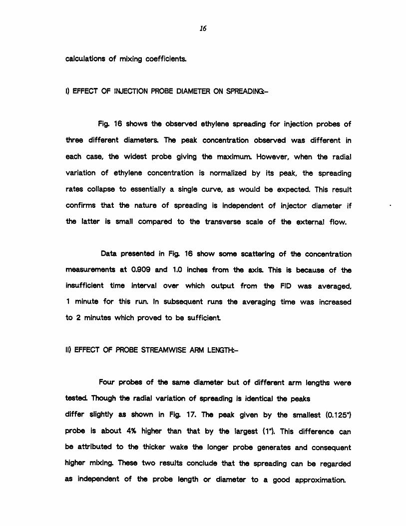
I) EFFECT OF INJECTION PROBE DIAMETER ON SPREADING-

Fig. 16 shows the observed ethylene spreading for injection probes of

three different diameters. The peak concentration observed was different in

each case, the widest probe giving the maximum. However, when the radial

variation of ethylene concentration is normalized by its peak, the spreading

rates collapse to essentially a single curve, as would be expected. This result

confirms that the nature of spreading is independent of injector diameter if

the latter is small compared to the transverse scale of the external flow.

Data presented in Fig. 16 show some scattering of the concentration

measurements at 0.909 and 1.0 inches from the axis. This is because of the

insufficient time interval over which output from the FID was averaged,

1 minute for this run. In subsequent runs the averaging time was increased

to 2 minutes which proved to be sufficient

II) EFFECT OF PROBE STREAMWISE ARM LENGTH:-

Four probes of the same diameter but of different arm lengths were

tested. Though the radial variation of spreading is identical the peaks

differ slightly as shown in Fig. 17. The peak given by the smallest (0.125")

probe is about 4% higher than that by the largest (1"). This difference can

be attributed to the thicker wake the longer probe generates and consequent

higher mixing. These two results conclude that the spreading can be regarded

as independent of the probe length or diameter to a good approximation.

The effect of finite diameter and length of the injector is to make the

tracer gas appear as if it is originating further upstream than the actual

location of the injection probe. The apparent origin was located by two

methods. One was by tracing the half concentration width at several locations

downstream and extrapolating towards the injector to find the point of zero

half width, which is the apparent origin. The second was by measuring and

extrapolating the peak concentration to give the point of 100% of injected

concentration. From the first method the apparent origin was calculated to be

1.7 radii upstream of its actual position. This equals roughly 2% of spreading

distance. The second method gives 1.1 radii. In mixing coefficient calculations

the result from the first method was used, as it was thought to be more

accurate than the other.

The effects of external velocity and turbulence levels on the

spreading level were next investigated. In these measurements an injection

probe of 0.041" inner diameter, 0.059" outer diameter and 0.50" arm length

was used. Ethylene was injected at 2.05 lit/min which gives an exit speed of

40 m/s based on the inner diameter of the injecting probe, or 19.5 m/s when

based on the outer diameter of the probe. The term "injection velocity" will

refer to the latter speed (19.5 m/s).

III) EFFECTS OF EXTERNAL TURBULENCE LEVEL.-

Ethylene was injected into the jet at four axial locations.

i) At 2.25 jet diameters downstream of the orifice where the turbulence

level is roughly 3%. This region is in the potential core of the jet As shown

in Fig. 18 the spreading here is affected very slightly by external jet

velocity. The observed turbulence intensity of 3% is consistent with the

measurements reported by Antonia and Bilger [Ref. 18]

ii) At 10.25 diameters downstream where the local turbulence is

roughly 10%. The halfwidth of concentration curves in this case is larger

and spreading is sensitive to external jet velocity variations as shown in

Fig. 19.

iii)&iv) At 18.25 and 28.25 diameters downstream where the local

turbulence levels are roughly 18 and 25%. Again the half width increases with

turbulence and is sensitive to external jet velocity changes as shown in Fig.

20 and 21.

IV) EFFECTS OF EXTERNAL STREAM VELOCITY

To investigate the effects of external jet velocity on spreading, jet

velocity was varied between 5 and 60 m/s in case (iv), while the injection rate

was kept constant The half width was a minimum when the jet speed was closest

to that of injection. It increases with the difference in velocities of

injection and the jet, (nondimensionalized by the jet velocity). The results

are shown in Fig. 21.

ESTIMATION OF MIXING COEFFICIENT:-

Mixing coefficients were calculated from equations (5) and (7) using

the half concentration widths as the measure of the radius of spreading. Fig.

22 shows the calculated mixing coefficient as a function of local jet turbulence

level for two different jet velocities. Both plots show mixing coefficients,

calculated from the point source model and the free jet model, as a function

of external turbulence level, for values ranging from 3 to 25%.

Effects of changing the external velocity on the mixing coefficient are

shown in Fig. 23. This plot gives the mixing coefficient as a function of the

difference between external velocity and the injection velocity

nondimensionalized by the latter, i.e. (Vext - Vinj)Ninj.

SUMMARY OF RESULTS :-

Effects of probe characteristics on mixing were investigated.

Probe diameter and streamwise arm length have no appreciable influence on

mixing levels. External flow velocity and turbulence levels, however do affect

the rate of spreading of the tracer gas. A free jet model has been proposed

for relating tracer gas spreading to mixing coefficient

CHAPTER 4

INSTRUMENTATION AND EXPERIMENTALTECHNIQUEB

This chapter describes the experimental facility, instrumentation, data

acquisition and reduction techniques. Measurements of compressor speedline,

flow angles and turbulence levels are also reported.

4A COMPRESSOR AND RIG DESCRIPTION

The test compressor is a three stage, low speed compressor originally

used to research blading concepts for Pratt and Whitney. It is described in

detail by Christianson [Ref. 191 and Gamache [Ref. 201 The compressor has a

constant annulus flow path with inner diameter of 21.12 inches, outer

diameter of 24 inches (hub to tip radius ratio of 0.88). Aspect ratio averages

0.8 for the rotors and 1.2 for the stators. Specifications for the design

performance and blading are included in Tables 1 and 2.

All the tracer gas experiments were carried out in the build #4

configuration of the compressor. Specifications of this build are included in

Tables 1 and 2. A complete description of the facility is available in either

reference, and only a brief explanation is provided here.

Fig. 24 shows the compressor rig assembly. Room air enters a

bellmouth through a foreign object damage screen (FOD), located approximately

one compressor radius upstream of the IGV entrance. The flow passes through

the compressor, out through a constant height annular section about two

compressor radii in length. Downstream of this a conical throttle is used to

control mass flow rate. After the throttle, the flow enters a dump plenum,

and flow straighteners (consisting of two screens and a honeycomb section)

before encountering an orifice plate used to measure overall flow rate. The

flow then exits through a 90 degree elbow, and an exhaust fan. The fan was

off and its rotor locked in all the tests described in this thesis.

4.B DATA ACQUISITION SYSTEM

The data acquisition and control system used in this thesis effort

consists of several distinct parts. These are :

1) Computers : An LSI-11/23 and a Microvax-Il were used to control all data

acquisition, drive the two traversers and reduce and plot the results.

2) A/D Converter : A Data Translation DT2752 12 bit analog-to-digital

converter was used to digitize analog data on line. Analog data were not

recorded. An onboard programmable gain amplifier allowed resolution of the

converter to vary between 0.5mV and 4mV depending on the type of

measurement being made. All instrument calibrations were performed at same

gain level as the actual measurements.

3) Real-Time Clock : A Data Translation DT2769 programmable real time clock

was used as a time base generator for the A/D conversions.

4) Filters : TSI Model 1057 signal conditioners were used to filter the high

response data.

5) Traversing Unit : Two L.C. Smith trversing units were used to allow

computer-controlled positioning in radial, circumferential and yaw angle

motions of the hot wire sensors, cobra pressure probe and tracer gas

sampling probe. This allowed a fairly automated high and low response data

acquisition process. Accuracy of positioning using this unit was ±0.004 inches

in radial motion and ±0.2 degrees in circumferential motion and yaw angle

positioning.

6) Baratron Pressure Unit : All pressure calibrations were referenced to a

high accuracy MKS Baratron electronic pressure measurement system. The

differential pressure head has a range of 100 torr (1.93 psi) and pressure

could be read to an accuracy of ±0.0005 inches of water. The Baratron

unit had a digital output read directly by the computer.

7) Scanivalve : A scanivalve unit was used to acquire most of the pressure

measurements made on the compressor. A single Spectra strain gage type

transducer was mounted in the unit with a pressure range of ±5 psi. The

standard deviation of its calibration was 0.05 inches of water. This

corresponds to roughly 1.5% of mean dynamic pressure in the compressor.

8) Temperature Multiplexer : An Analog Devices uMAC-4000 temperature

multiplexer was used to acquire all thermocouple measuremenants. Type K

thermocouples were used for temperature measurements.

9) Torque Meter : A Lebow 1105-5K skip-ring torque meter is used for torque

measurement The meter is an integral part of the drive train, located between

the compressor and the output of the speed increasing drive belt assembly.

The torque meter also contained a sixty tooth gear used to measure RPM of

the compressor.

4C EXPERIMENTAL TECHNIQUES

1) HOT WIRE ANEMOMETRY

A single hot wire sensor was used to measure all the velocities and

the correlations for length scale calculations on the free jet An electronic

linearizer was used to make the anemometer voltage output directly proportional

to stream velocity, with the constant of proportionality determined through

calibration.

One source of error in taking hot wire data is shifts in the calibration

constant over a run time (typically 8 hours). These shifts are mainly due to

dirt deposition on the wire. Typically calibration slope could shift by 7%, which

introduces a ±3% error into velocity measurements. Temperature also affects

hot wire calibration. At a typical overheat ratio of 2 (sensor operating at

about 4500F), a 200 F temperature rise corresponds to a 1% drop in indicated

velocity. Corrections to measured velocities were made by assuming that any

shift in the calibration constant was linear with time.

2) MASS FLOW CALIBRATIONS

Although it is possible to use a calibrated inlet to measure flow rate

while the test compressor is operating unstalled, it was more convenient to

use the orifice plate pressure drop. The calibration procedure for this method

was documentd by Lavrich [Ref. 21] The form of the calibration is :

C C .............. .... (10)

where

C, - average axial velocity in the compressor annulusC - Reynolds number dependent calibration constantAP - the orifice plate pressure dropPop - the air density in the ductp - the ambient air density.

3) ENSEMBLE AVERAGING

Ensemble averaging was required for all velocity measurements taken

with high response instrumentation. This averaging must be done judiciously

in order to not throw away important information. A signal from a probe is

composed of three distinct parts. The first one is the D.C. value of the

signal, the next one is a sum of all signals that occur at distinct frequencies

and the last is the noise and random event portion of the signal. The third

part includes turbulence and other unsteadiness of random nature. Averaging

is performed to increase signal-to-noise ratio for a given measurement

For measurements on the free jet, where the second part of the signal

is absent, the difference between the total signal and the average gives the

instantaneous randomly fluctuating component (turbulence) of the velocity.

However the second component was present for measurements in the compressor

in the form of rotor wakes at blade passing frequency. Calculation of turbulence

in this case required that along with the D.C. component this frequency be

also subtracted from the total signal. A more detailed discussion can be found

in [Ref. 22]

4JD COMPRESSOR PERFORMANCE

Locations of the instrumentation used in the following measurements

are shown in Fig. 25. Inlet and exit total pressures were measured with rakes

of kiel head total pressure probes at four circumferential locations. Inlet and

exit static pressures were measured at both inner and outer radii at four

circumferential positions. Interrow static pressure taps were located on the

outer wall at a single circumferential location. Temperatures were measured

with type K thermocouples at 50% span at each interblade position. All pressure

measurements were made using the scanivalve unit Overall performance was also

measured by a direct differential pressure measurement with the Baratron unit

Inlet total to exit static pressure difference, normalized by mean blade

dynamic pressure, is a useful performance measure. The total to static

pressure coefficient is defined as :

Ps9-Pt2-ts - 0.5pU 2 . . . . . . . . . . . . . . . . . . . . . . . (11)0.5pU 2

where the numbered subscripts refer to axial measurement stations shown in

Fig. 25.

Normalizing data by this factor, for low tip Mach numbers, the data at

different speeds collapse sufficiently to a single curve. Total to static pressure

rise coefficient versus flow coefficient data is shown in Fig. 26. Data were

taken at three different rotational speeds : 1200, 1800, 2400 RPM giving a

Reynolds number range of 0.83 x 105 to 1.66 x 105 based on average blade

chord, and a tip Mach number range of 0.11 to 0.22.

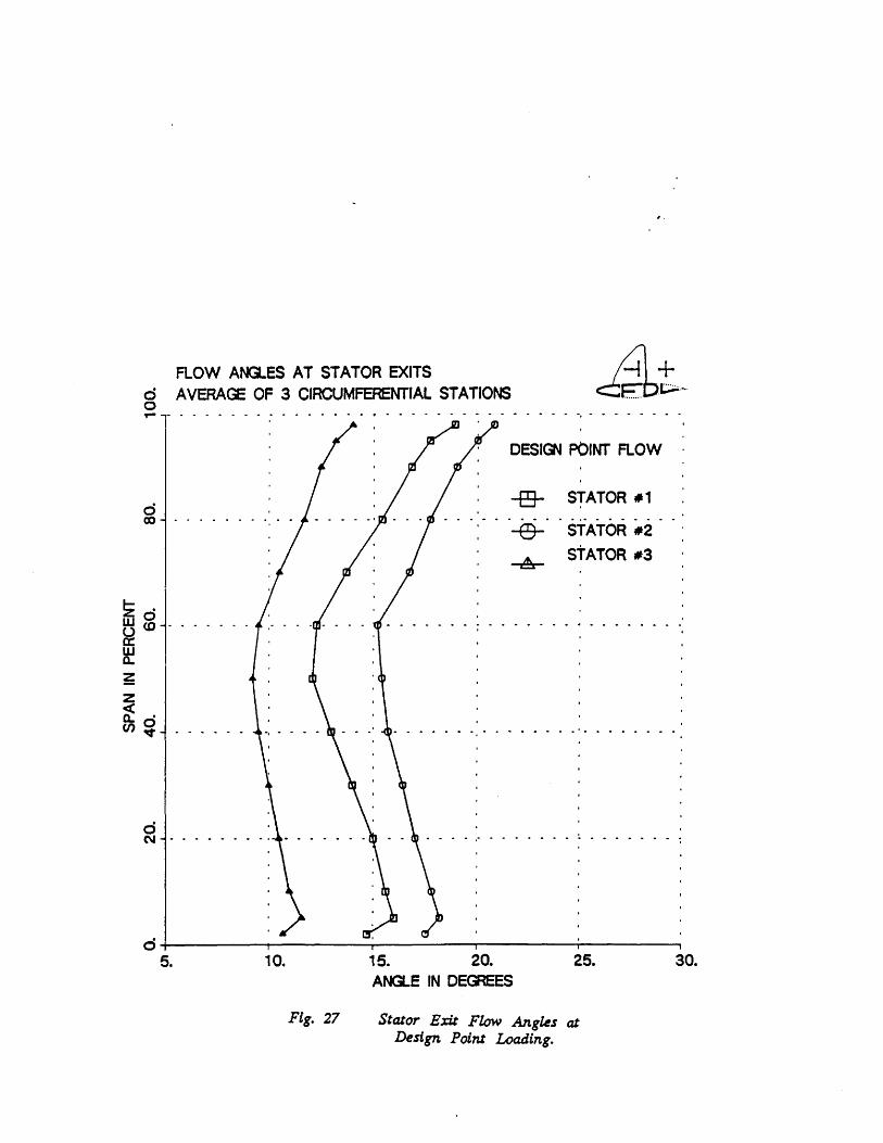
Flow angles behind each rotor were measured using a self-nulling

cobra probe at several spanwise locations. The cobra probe consists of three

total pressure taps. The outer two holes are perpendicular to each other and

the middle one bisects the angle between them. The pressure difference

between the two outer probes is sensed by a pressure transducer and an

actuator rotates the probe until the pressure difference is nulled. Fig. 27 and

28 show the flow angles at design point flow and at a higher loading.

Turbulence levels (the fluctuating part of the velocity signal as

defined in the ensemble averaging technique) were measured in front of each

of the three stators and the IGV at mid-pitch locations. Fig. 29, 30 and 31

show the turbulence levels for design point flow and at a higher loading

upstream of the three stators respectively.

A detailed description of the results of the tracer gas experiments

in the compressor is included in the next chapter.

CHAPTER 5

TRACER GAS EXPERIMENT

This chapter describes the tracer gas experiment carried out on the

low speed compressor. Measurements were taken at design point (flow coefficient

- 0.5) and at an increased loading (flow coefficient - 0.42). These two

points were marked on the compressor speedline in fig. 26.

5A ETHYLENE INJECTION AN) SAMPLING PROCEDURE

Ethylene was injected at selected locations in the compressor flow

field and detected downstream. The sampling probe was traversed in a grid like

network of span and pitchwise locations. The concentration output of the FID

was then reduced to a set of contour plots, one set per each injection. The

contour plots of constant ethylene concentration are used to display the

spreading patterns of ethylene in the sampling planes.

As mentioned earlier, one aim was to investigate the evolution of the

mixing process. This meant that spreading was to be observed across each of

all three stators, all three rotors and all three stages individually. In each case

ethylene was injected at various spanwise locations, some close to the

endwalls and some in the mid-span region so that effects of both secondary

flows and turbulence could be looked at The pitchwise location of injection

was found to be unimportant when spreading across a rotor was investigated. For

observations across stators and IGV, injection was done at several pitchwise

locations.

The injection probe was mounted on a L.C. Smith actuator, driven by a

computer, with radial and yaw motions. In all the cases discussed above

injection was done 1mm upstream of the leading edge plane of the respective

blade row and sampling was accomplished 1mm downstream of the trailing

edge plane of the corresponding blade row. ( For reference Imm corresponds to

roughly 3% of stator chord, 2% of rotor chord and 5% of IGV chord. ) The

sampling probe was mounted on a second actuator with radial, circumferential

and yaw motions, though only two motions can be performed at any one time.

This actuator was also automated.

At each injection location the direction of injection was adjusted to

align with that of the local flow using a three head cobra probe discussed

in chapter 4. The speed of injection was matched with the local flow speed.

Local velocity was measured using the middle head of the cobra probe for

total pressure and a linear interpolation between the outputs of the static

pressure taps on the hub and the casing. Velocity matching was not possible

for injections close to end walls (within 6% of the span), because at these

velocities ethylene flow was smaller than that necessary for good FID and

flowmeter resolutions.

Similar flow angle adjustments were made in sampling probe positioning

also. The was not completely nulled owing to the large number of data points

and time involved. Nulling typically takes about 10 iterations and 30 seconds.

Only the first two iterations were allowed during sampling. The sampling probe

was connected to a suction pump and the suction rate was kept a constant for

each injection. No velocity matching adjustments were made during sampling

since the sensitivity of the FID changes with the sample flow ratý as discussed

in chapter 2. However, Wisler et al [Ref. 5] tested sampling at several

different rates and reported that the suction speed did not significantly

alter the measurements.

The settling time of the FID was greatly decreased compared to the

free jet experiments, because the FID could be placed much closer to the

sampling probe, and thinner tubing could be used to carry the sample from the

probe to the FID. Settling time was roughly about 15-20 seconds.

The probes used for injection and sampling were picked from those

tested in chapter 3. As mentioned in that chapter all the probes were 'L'

shaped. The probe selected for injection had a streamwise arm length of 1/8

inches, inner diameter of 0.023 inches and a wall thickness of 0.01 inches. The

sampling probe was of the same arm length and had a diameter of 0.033 inches

and a wall thickness of 0.012 inches. Volume flow rate, based on outer

diameter, is denoted by injection speed, or sampling speed.

The sizes of the radial and circumferential movement increments of the

sampling probe were dictated by the relative change of ethylene concentration

with position. If the ethylene concentration increased or decreased rapidly,

sampling probe movement increments were decreased in length; this was

necessary in the vicinity of maximum ethylene concentration.

5.B DATA REDUCTION PROCEDURE

Data for concentration contour plots were acquired by recording the

voltage output from the FID and the radial and pitch positions of the sampling

probe relative to a reference point The voltage output of the FID was

converted into concentration using a calibration curve. One contour plot was

made for each injection point, requiring roughly an hour of data taking.

The contours were plotted on a background grid which is in the shape of a

passage between two adjacent blades in a blade row. ( Note that the pitch

differs from one blade row to another. ) All contours were plotted on a grid

of 100 units in span and 100 units for convenience. A polynomial interpolation

routine was used in plotting to generate points of desired concentration.

At flow speeds in the compressor, and distances over which spreading

was observed, molecular diffusion of ethylene into air can be assumed to be

negligible [Ref. 231 ( The diffusion length is roughly 0.5% of the convected

distance. ) Thus, the movement and spreading of ethylene are solely due to

the action of the compressor flow and turbulence.

5.C RESULTS OF ETHYLEIE TRACING MEASUREMENTS

Fig. 32 and 33 show contour plots for spreading across the first

stator, at design point and at increased loading respectively. The next two

figures, 34 and 35, show the contour plots for the first rotor at the two

flow conditions. Since these contour plots are similar to those of the

other rotor stator rows (as will be shown) we can discuss them as

representatives of the situation throughout the compressor.

Consider the spreading due to injection at mid-span, mid-pitch location

in front of the first stator at design point in Fig. 32. The contours are almost

circular with centers moved towards the suction side by roughly 2% of the

pitch. This movement of the core, though small, is present in all three

stators. It is probably due to the pressure difference between the pressure

and suction surfaces of the adjacent blades. The symmetric spreading of ethylene

can be attributed only to turbulent diffusion. Contour plots due to injections

at 25% and 75% of span at mid-pitch are also remarkably symmetric. Thus it

seems that in the mid-passage region only turbulence is the cause of ethylene

spreading.

Contours close to the blade surfaces or to the end walls are distorted.

One can not say, just from the contours, whether the distortion is due to

secondary flows or anisotropies in turbulence. A qualitative analysis can

however be provided by scaling the one-dimensional diffusion equation. The

differential equation is :

= •.................. (12)ax y

where 'u' is the velocity in a direction '', which is perpendicualar to 'y' and 'e

is the diffusion coefficient

For a fluid particle, whose motion can be described by this equation,

the time ' t ' taken to diffuse through a transverse distance 'y', during which

it would have travelled a distance 'u' in the x direction , is given by :

t - o(x/u) ...... ......... (13)

and also

t - o(y 2 /e) .................... (14)

Equations (13) and (14) applied to the contours for mid-pitch and

mid-span location imply a mixing coefficient of 0.0035 m2/s. According to Fig.

22 this corresponds to a 8% turbulence level. This number is in reasonable

agreement with the measured turbulence level for this location, which from

Fig. 29 is 6%. The analysis is consistent with measurements, and the

implication is thus that, at this location, spreading is due to turbulent

diffusion.

These arguments can be applied to a set of distorted contours, say

90% span and 45% pitch. These yield a mixing coefficient of 0.008 m2/s.

According to Fig. 22, based on the free jet model discussed in chapter 4, this

corresponds to a 18% turbulence level. However, the measured turbulence

level for this location, from Fig. 29, is 10-11%. This implies that some

other mechanism (secondary flows and/or anisotropies in turbulence) must

be involved to account for the mixing at this location. In other words, at

this location contributions from turbulence and other effects are of similar

magnitudes.

At increased loading the wakes become thicker and the turbulence

level increases. Contours at increased loading show increased spreading as

seen in Fig. 33. This is true for both the more symmetric and the distorted

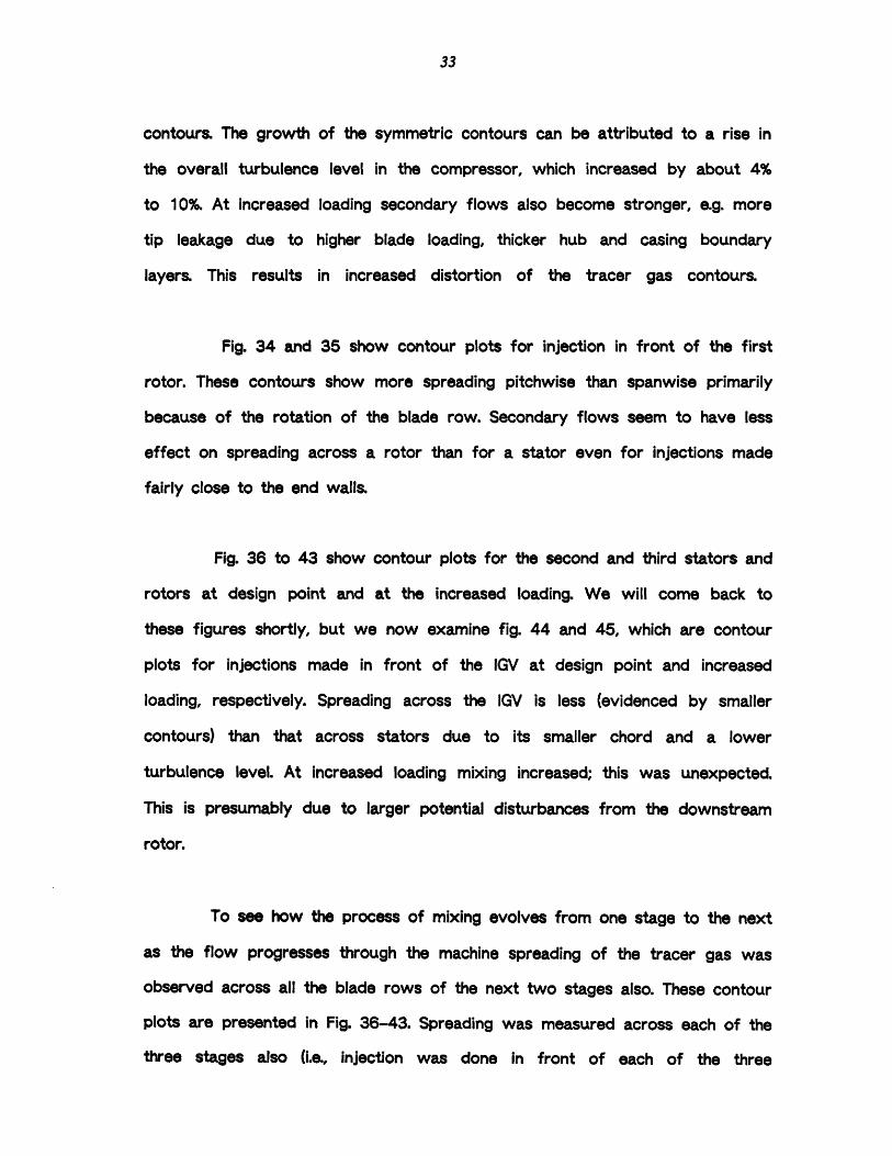
contours. The growth of the symmetric contours can be attributed to a rise in

the overall turbulence level in the compressor, which increased by about 4%

to 10%. At increased loading secondary flows also become stronger, e.g. more

tip leakage due to higher blade loading, thicker hub and casing boundary

layers. This results in increased distortion of the tracer gas contours.

Fig. 34 and 35 show contour plots for injection in front of the first

rotor. These contours show more spreading pitchwise than spanwise primarily

because of the rotation of the blade row. Secondary flows seem to have less

effect on spreading across a rotor than for a stator even for injections made

fairly close to the end walls.

Fig. 36 to 43 show contour plots for the second and third stators and

rotors at design point and at the increased loading. We will come back to

these figures shortly, but we now examine fig. 44 and 45, which are contour

plots for injections made in front of the IGV at design point and increased

loading, respectively. Spreading across the IGV is less (evidenced by smaller

contours) than that across stators due to its smaller chord and a lower

turbulence level. At increased loading mixing increased; this was unexpected.

This is presumably due to larger potential disturbances from the downstream

rotor.

To see how the process of mixing evolves from one stage to the next

as the flow progresses through the machine spreading of the tracer gas was

observed across all the blade rows of the next two stages also. These contour

plots are presented in Fig. 36-43. Spreading was measured across each of the

three stages also (i.e., injection was done in front of each of the three

rotors and sampling was done immediately downstream of the corresponding

stator). Fig. 46-51 show these contour plots.

The central point shown by all these figures is that spreading across

all the three stators looks very similar, as does spreading across all three

rotors. There is little evolution of mixing from one stage to the next

Further the same conclusion can be drawn from contours plotted for spreading

across a whole stage. This conclusion was independently drawn by Li and

Cumpsty [Ref. 6] where it was shown that the spreading across first and

second stators was similar and that the mixing coefficients were roughly

the same. Note that the distortions observed in stator related contours appear

to be less prominant in these plots, because they are now combined with a more

uniform spreading pattern. The distortions themselves diffuse out as the

flow progresses through the rotor.

Based on the contour plots, a mixing coefficient was calculated

for each injection. First the average distance (radius) of each contour

from its core (maximum concentration point) was calculated. Next a least

square fit was obtained between concentrations of the contours and their

average radii. In obtaining the least square fit each contour was wighted by

the number of data points it contained. One set of points from this fit was

used in equations (5) and (7) for ' C ' and ' r '. Mixing coefficients thus

obtained were normalized by the product of axial velocity and the axial

distance over which spreading was observed. The nondimensionalized coefficients

were plotted in Fig. 52-61 as functions of span.

Fig. 62 shows the evolution of mixing in the compressor. In this figure

the mixing coefficient was plotted for four different cases for each blade row:

at midspan and at end-wall for design point loading and at increased loading.

The mixing coefficient was normalized independently for each blade row by

local relative velocity and blade chord. (The author is grateful to Dr. Koff

for this suggestion.) The difference in the magnitudes of the mixing

coefficients for stators and rotors is smaller than using the previous

normalization, but the rotors still have larger mixing coefficients. For

reference mixing coefficients corresponding to 6% turbulence (the level

measured in the mid-span mid-pitch region at design point loading ) and 11%

( measured near end-walls at design point loading ) are also indicated.

In Table 3 normalized mixing coefficients and corresponding aspect

ratios from [Ref. 10,11] were summarized along with our results. No clear trend

in mixing as a function of aspect ratio can be oserved.

The next chapter gives a summary of the conclusions derived from

this data. at is given. Some recommendations for future research in this

field are also included.

CHAPTER 6

CONCLUSIONS AND SUGGESTIONS

The work described in this thesis consists of an experimental

investigation of mixing in a three stage axial compressor. The evolution

as flow progresses through the machine was examined. Research was also carried

out to quantify the effects of injection probe geometry, turbulence level,

injection and free stream velocity difference, and integral length scales on

spreading rates of the injected species.

6A CONCLUSIONS

Based on the tracer gas measurements the following trends in

mixing in the multi-stage compressor can be inferred :

Fluid migration and mixing are the combined effects of turbulent

diffusion and secondary flows. The relative importance of each of these

mechanisms depends on the location in the machine.

In a stator row turbulent diffusion dominates in the midpassage

region. However, near the end walls and close to the blade surfaces secondary

flows can also make appreciable contributions to mixing.

Turbulence is more important in mixing across a rotor than across a

stator. Thus effects of secondary flows are less noticeable in the rotor even close

to end walls.

At increased loading there is more mixing in both stators and rotors.

Contributions from secondary flows become more significant at increased

loading.

Mixing across all three stators is very similar, as is mixing across

all three rotors. There is little evidence of evolution of the mixing process.

Flow distortions generated in one blade row do not affect mixing in the next

blade row to any significant degree.

Mixing coefficients for rotors based on relative velocity and

blade chord are in general larger than those for stators. (For the geometry

examined they are roughly twice that for stators.)

Measurements of the effects of probe and external flow parameters

on the spreading of the injected species show:

The length of the injection probe has little effect on the level of

mixing, even when comparable to the distance over which the tracer gas

was allowed to spread.

The diameter of the injection probe does not affect the spreading

pattern.

Turbulence level of the external flow has a strong effect on

the mixing coefficient

The mixing coefficient changes with the velocity difference between

the mainstream and the injection speed. Mixing is a minimum when both

velocities are equal (with the injection velocity defined as the volume flow

rate per unit area based on the outer diameter of the probe).

The integral length scale of the main stream does not affect the

level of mixing strongly, at least within the range of the length scales that

was investigated.

6.B SUGGESTIONS FOR FUTURE RESEARCH

The results of the present research provide some more insight into

understanding the mixing process in multi-stage axial compressors. However

some important issues remain unresolved. It is suggested that this process

be investigated further as detailed below.

A detailed measuremnt of the secondary flow field in a blade row

would be helpful in determining whether it is indeed the secondary flows

that cause distortions in the tracer gas concentration contours. Once this

is done a method needs to be devised to separate the effects of turbulence

from those of secondary flows so they can be modelled separately, thus more

accurately, using [Ref. 2] and equation (7). It is suggested that streamline

tracing using three dimensional computational procedures would be useful in

this regard.

The experimental results indicate that secondary flows generated in

one blade row diffuse out (or mix out some other way) before the flow

approaches the next blade row. Most of this must clearly be happening in the

spacing between the two rows, similar to wake mixing. This process should be

investigated to see how exactly this diffusion takes place and how it is

affected by varying the inter-row gap.

Any kind of mixing introduces extra losses. But the mixing process in

axial flow machines takes away high loss fluid from the end walls and

redistributes it all over the annulus. Thus it decreases profile losses while

introducing some losses of its own, the balance being to our benefit This

observation raises the question as to whether enhancing mixing by some

artificial means would decrease the overall losses. If so, it is definitely

worthwhile to find out by how much.

With the data presented in this thesis, mixing measurements are

available for four machines. Emphasis should thus be shifted to analysis.

Models that can compute the parametric dependence of the mixing coefficient

on various flow parameters, e.g. loading level, blade-wake thickness, pressure

gradient, etc. and machine parameters, e.g. aspect ratio, tip clearances, inter

blade row gap, etc. should be investigated.

Efficient methods to incorporate mixing coefficient into through-flow

calculations should devised.

Compressor Design Specifications (Bld 4)

Number of stages 3Tip diameter [in] 24.0Hub-to-tip radius ratio 0.88

Static Tip Clearance [in] (measured)

Rotor 1 0.032

Rotor 2 0.030Rotor 3 0.034

Static Hub Clearance [in] (measured)

IGV 0.002

Stator 1 0.030Stator 2 0.036Stator 3 0.038

Design Average reaction

Design Flow Coefficient

Total Pressure Rise Coeff. (measured)

0.65

0.501.46

Table 1

Compressor Blading Design [Bid 4]

No. of Blades

124

54

85

55

88

49

90

Chord [in]

0.826

1.779

1.235

1.764

1.232

1.996

1.235

Aspect Ratio

1.746

0.811

1.168

0.817

1.170

0.722

1.168

Camber [deg] Stagger Angles

11.0 13.1

17.0 44.3

27.0 26.0

18.0 45.5

25.0 28.0

20.0 46.6

53.0 20.5

Table 2

IGV

Rotor 1

Stator 1

Rotor 2

Stator 2

Rotor 3

Stator 3

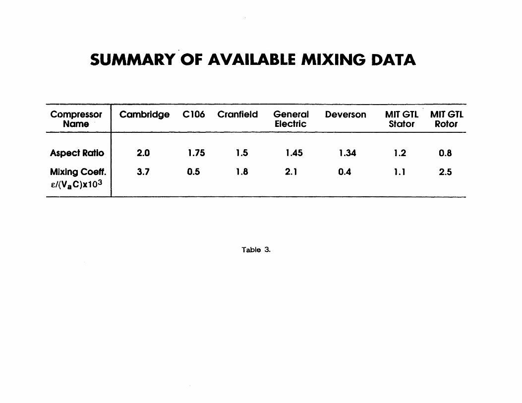
SUMMARY OF AVAILABLE MIXING DATA

Compressor Cambridge C106 Cranfield General Deverson MIT GTL MIT GTLName Electric Stator Rotor

Aspect Ratio 2.0 1.75 1.5 1.45 1.34 1.2 0.8

Mixing Coeff. 3.7 0.5 1.8 2.1 0.4 1.1 2.5E/(VaC)xl03

Table 3.

Exhaust toAtmosphere

Fig. 1 Tracer Gas Detection System.

Acknwl. Denton and Usui [Ref. 61

Sam;Pro

C2H4Cylinder

eler

Exhaust toAtmosphere

Flame Chamber

IguitionCoil

Electrode

CoAi

SampLe ~

Flame Ionization Detector.

II I

%616 Wow-"

Fg. 2

iC mn aVhln ka~i Su at* p41

Sample Pressure Above Ambient in Psi.

Fi. 3 FID Respona to Sample Pressure Variations.

40

C

0.00

m

FID Response to Variation in Hydrogen Flow

(U-

1.375 i.750 i2125 2.500 3.825 4000

Hydrogen Pressure Above Ambient in Psi.

Fig. 4 FID Response to Hydrogen Pressure Variations.

2.875 3250

.... .. . . . . . . . . . . . . . ... . . . . . . ... . . . . . ... . . . . . . . .. . . . . . ..

~b·p

..............

. . . . . . . . . . . . . .

................................

0001.v

Response to Varitaon In Air Flow

°

...................... .

0.00 0250.50 0.75 tOO 1.25 1.50 1.75 2.000.50 0.75 1.00 1.25 1.50 1.75 2.00

Air Pressure Above Ambient in PsL

Fig. 5 RD Response to Air Pressure Variatiors.

4 .a tL;RIO

i,-o •

Linearity of FID Responseo.r=--

.. . . . . . . . . . . . . . . . . . . ..- -

Fig. 6 Linearity of FID Signal.

I-

0

oqC

O

ca

00. 50. 100. 150. 200. 250.

% of Ethylene Concentration x 100.

I

I

I

I

I

FID

R

ESPO

NSE

IN

P.

P.M

.

221.

72

25

.0 140.0

290.

0296.7

303.3

31

0.0

21

5.8

218.3

143.3

bi

O O (3 o• o•

14

6.7

150.

0

O O O o O J

I Urg I

H3 If-- 1

I I--- - - -~-----

f ,r

Up - Injection Velocty

Us - External Stream Velocity

Ux - Total Axial Velocty

Ur - Radial Velocty

d - Jet Di~mwter

Fig. 8 Schematic of Injection from a Jet into a Uniform Stream.

X/M (X-0 IS MESH LOCATION

Fig. 9 Streamwise Variation of Turbulence Intensity

in a Wind-tunnel Fitted with Screens.

v' ALOIG TLELL CEE~I V-32m/l

I

50.

/l-+

v' AT X/M-30 ALONG TUNNEL WIDTH:; V-32m/s.MESH SIZE: M-1.0".d-0.254

>cO

lad

-2.0 -1.5 -1.0 -0.5 0.0 0.5Y/M (Y-O IS TUNNEL CEFNTELINE)

Fig. 10 Highest Turbulence Level Achieved in Wind-tunnel.

1.5 2.0Nm

v' ALONG TUNNEL WIDTH. AT X/M-20,V-32 m/s.MESH SIZE-1.0",d-0.207"

.500 -1.125 -0.750 -0375 0.000 0375 0.750 1.125 1.500Y/M (Y-0 IS TUNNEL CENTERLIME

Fig. 11 Profile of Nonuniform Turbulence Intensity.

-1

VELOCITY PROFILES OF THE JETAT THREE CROSS SECTIONS: X/d-29.25,35.25,39.25

Y/d (Y-O IS JET AXIS)

Fig. 12 Test of Symmetry of the 1" Round let.

'4

L

VELOCITY PROFILE OF THE JETDIAMETER OF JET NOZZLE-1.0"

0.X/d ALONG THE JET AXIS

Fig. 13 Velocity Profile of the Jet.

TUICE O(4ARACTCITICS OF TM .rtu' VS U JxLCALW N VJ.

i o10. 1 iTa isX/d ALON THE .rT AXIS

3 a& 40.

iBUUCE I SELF PISERVI~ FUMONu ALON3 CoWT. YIX LM

- ylx-O.10736

c-OA.07643

-'yx-.0eas4s

i0w 23.71 27s.0 31.25 3500 8. 42.50 4--00X/d

Fig. 14 Turbulence Intensity In the Jet.

C2 ·

:iz

ql

g~.

AUTO CORR PLOTSX/d-25.25.Y/d-0.0

Variation of Length Scale Along Jet AxisNormalized by Jet Diameter.

Distance from Jet40. 45. 50.

IN msl

FIG 15 Length Scales in Similarity Region of the Jet

SQRT(T

V (JET) =20M/S: V (INJ) =20M/S: X (INJ) /D=28.25:L (INJ) =0.5"

% -&- DIA (NJ -0.023"

0"(:3

00

00

0

0(D

o00

-e- DIA(INJI=0.033"rl

-1.00 -0.60 -0.20 0.20 0.60DIST. IN INCHES

Fig. 16 Effect of Injection Probe Diameteron Tracer Gas Spreading.

1.00

V (JET] =20M/S:V [INJ =20M/S:X [INJ) /0=28.25:IR [(INJI=0.04]"

- L (INJ) -1.00"- L (INJ) =0.75"-- L (INJ)= O.50"

00

CO

0Oo

Z

zO

0

NO

'-1.00 -0.60 -0.20 0.20 0.60 1.00DIST. IN INCHES

Fig. 17 Effect of Injection Probe Lengthon Tracer Gas Spreading.

Potential CaseV(INJ) =20M/SX(INJ)/D=2.25L(INJ) -0.50"T'r% . ^%Al

m

DIST. IN INCHESFig. 18 Effect of Turbulence on Tracer Gas

Spreading; Case-I : Potential Flow

V (JET) -I50/S-O V (JET) -q0h/S

zZ

ID

.00

Turbulence Level = 10%

V(INJ) =20M/SX(INJ)/D=10.25L(INJ) -0.50"rT % 1TVI r N-r% ) A1 9

- V (JET) 50M/S-0- V JET) -, OM/S

00

O0 -0.60 -0.20 0.20 0.60 1.00DIST. IN INCHES

Fig. 19 Effect of Turbulence on Tracer GasSpreading; Case-II : 10% Turbulence

-1.C

v

Turbulence LevelV(INJ) =20M/SX (INJ) /D=18.25L(INJ) =0.50"nTh 1TnT1= n on*

-- V (JE-T) 504//S- V JET) *O.//S

DIST. IN INCHES

Fig. 20 Effect of Turbulence on Tracer GasSpreading; Case-III : 18% Turbulence

V (INJI =20M/S:X (INJ) /D=28.25:L (INJ) =0.50":ODIAR (INJ) =0. L01"

-6- V (JET) 5M/S-* V (JET) -60M/SH-t

00

V (JET)V (JET)V (JETI

-1.00

-5DM/S-'on/S-30M/S

-0.60 -0.20 0.20 0.60DIST. IN INCHES

Fig. 21 Effect of Turbulence on Tracer GasSpreading; Case-IV : 25% Turbulence

1.00

MIXING COEFFICIENT VS. TURBULENCE LEVEL

V (JET) =20/S: V (INJ) =20M/S

-6- POINT SOURCE

La-

0

z

.X

V (JET) =lOM/S:V (INJ) =20M/S

-6- PO]NT SOURCEC1

LOCAL TURD. LEVEL

Fig. 22

LOCAL TURB. LEVEL

Variation of Mixing Coefficient withTurbulence Level.

MIXING COEFFICIENT VS. VELOCITY DIFFERENCEX(INJ) = 28.25; TURB. LEVEL = 25% FOR ALL POINTS

0 - POINT SOURCE

7.0

X

U-

U.,

ZzX

NONDIM. VEL. DIFF.

Fig. 23 Variation of Mixing Coefficient withMain Stream Velocity.

00

Low Speed Multistage Compressor

DumpPlenum

Test Facility

Low Speed Compressor Rig Schematic.Fig. 24

Total Pressure Rake k e

Static Pressure Tap (O.D.)0 Static Pressure Tap (ID.)

O Thermocouple

0 100 Arc Instrumentation Slot

t@ Inlet Struts

0 Exit Struts

0 @@@)ý51 4 g0

Exit

K) rf) CCV C\ (D(n (r (f) M (f) Ir -

- 0

--

Inlet Bellmouth

Fig. 25 Steady-state Measurement Locations.

1800

2250

2700

3150

0

450

900

1350

1800

I

o BLD•4 SPEEDLINEo

F °

0o

o

0

0

0.. . . . .------C

b0

0.800

-4-c;-

0.200 0.275 0.350 0.425 0.500 0.575 0.650 0.7250.200 0.275 0.350 0.425 0.500 0.575 0.650 0.725

inlet phi

Fig. 26 Total to Static Pressure Performance.

............

--- --

..

.. . . . . . . . el

FLOW ANGLES AT STATOR EXITSd AVERAGE OF 3 CIRCUMFERENTIAL STATIONSo

DESIGN POINT FLOW

- STATOR #1

STATOR #2STATOR #3

15. 20.ANGLE IN DEGREES

25. 30.

Stator Exit Flow AnglesDesign Point Loading.

cj6

a-zz

cf)

10.

Fig. 27

I ·

....... ...... .I .. ......

- - - · - -:

-I~ ·FLOW ANGLES AT STATOR EXITSd AVERAGE OF 3 CIRCUMFERENTIAL STATIONS0

CREASED ..OADINGSTATOR #1

STATOR #29-STATOR #3

15. 20.ANGLE IN DEGREES

25. 30.

d00-

6

zz3CM-

vCJ-

10.10.

Fig. 28 Stator Exit Flow AnglesIncreased Loading.

V-. . . . . . . . . . . . . . . . I . . . . . . . . . . . . . . . .. . . . . . . . .

TURBULENE KFENSITY (~A+

L..~. ..

z 4. 6. 8. 10. 12. 14. 16.RMS(uI/Ua

Fig. 29 Radial Variation of Turbulence LevelsUpstream of 1st. Stator.

so

-

- - -

I

'·

TURBULENCE ITENSITYIN FRONT OF 2ND STATOR

20.02.5 5.0 7.5 10.0 12.5 15.0 17.5RMS(u')/Ua

Fig. 30 Radial Variation of Turbulence LevelsUpstream of 2nd. Stator.

...............

~b~c

TURBULENCE INTENSITYIN FRONT OF 3RD STATOR

2.5 5.0 75 10.0 12.5 15.0 17.5RMS(u)/Ua

Fig. 31 Radial Variation of Turbulence LevelsUpstream of 3rd. Stator.

20.0

·

. . . . . . .. .

. . . . .. ... .

. .. . . . ... .

...............

...............

_

i . .. .

,•,

~b·c

.

DIAGRAM ILLUSTRATING THE COMPRESSORPASSAGE USED IN CONTOUR PLOTS

-50 PITCH 50 100-100

TIP

HUB

injections at(0,50) and (0, 5)

Pitch 100injections at(-45,50) and (45,50) injections at

(0,25) and (0,75)

injections at(45,5) and (-45,5)

Fig. 32 Contour Plots for Tracer Gas

injections at(0,90) and (-45,95)

CONTOUR LEVELS:97.80,60.4e,20

Spreading Across 1st. Stator at Design Point Loading.

-100

Tip

span

Hub

injections at(0, 98) and (0,2)

Pitch 100 injections at(45,50) and (45,90)

injections at(0,90) and (0,10)

injections at(-45,90) and (-45,10)

injections at(45,10) and (-45,50)

Contour Levels:97, 80, 60, 40,20

Fig. 33 Contour Plots for Tracer Gas Spreadi•g Across 1st. Stator at Increased Loadtng.

-100

Tip

Spa

R•--

COMNTOU PLOTS PMo K8CTO AT (I0.7 O AN0 .UPSTIAM CP 1ST RDITO

COMIM PLOTS RCI KCtfli AT M(01 ANO (,015LUPSTM O 1OST ROTIO

-100oo

lTT TIP

Wt-IP71~2IE

EfFFPALY1Ti-ri-4

LL(

I1j I

-9---

CON•OU PLOTS PCR NlCAtlMO AT (0.0 AO (25)UPSTAM Cr 1ST RIOTOL

-100

T1

WM I I 1..

401

".1-F

C=F

0=ic

7PI-

TP

5AP

7f

40

20

\Il

UrFig. 34 Contour Plots for Tracer Gas Spreading Across 1st. Rotor at Design Point Loading.

Contour Levels : 97,80,60,40,20.

100-T

Ir1m~Pr

ii

I ~I

FTI

EELi

111115

Ill

F

I -I r7

CONTUR PLOTS FOR KI CTIOM AT MM0#1

UPSTAM OF 1ST TOIC,

-100 r

I-

I-

~cl

-~I

dll I1

SPAN

I

t

rI-

ale

4U

~a #"U` 1

~' ~'

iI,

I

\r

-·

w·

~MHT· -- &P

t

iIs I

""

0

NC.ASE LOAMRcouros P.0! FOR ra3LW AT M0 ANDO 07LVSRmAM OF ST ODTI

-100TP

I

maul.I

HMl I

j•lAMsED LOAug

CONroWm PLS FOR rMci AT 0,M AoM 0.2WSTM.M CP 1ST AOTOf

ii

ii

SIANI I

201

PT

i

NcmASE LOADCOITOW"R OTS FOR KCTIGIO AT M0 ANOD ,10WIST•AM or IST IC•

100 -100 m

I IIi,

t=

--

-1CCONLcoasr

CH 100TPr

~F~R`,

HL7+F F

1I1I

I I ITF1 '4

EAD LOADICT"UR PLOTS POR IAMtI=n AT I.MMTFM OF 1ST RoIt

PITCH

FT7

1-1---

-1---

1j I

III

Fig. 35 Contour Plots for Tracer Gas Spreading Across 1st. Rotor at Increased Loading.Contour Levels : 97,80,60,40,20.

=FIN

KLLJI

~I I I

'hIi

47

t

II I I

-

r

r( (

R~L-(

L·v

mP

1 1 1i

'PT[1·

-- ·- -- -

IHLI · ' ' ' '

I I

rl

OONTOLm PLOTS FOR ~NCIx OIG AT (00) AND (05)LITPIMM OF 210 STATOR

-100 PITCH

TTI]

CONTOUR FLOTS FOR KECTIONS AT (025) AND (0,75)

UPSTIEAM OF 2N STATOR

100 -100_T

J1 Inil']I I II7 1 11

I II I

A I I/UX

PIFTc

NorOUR PLOTS FoR KWGIMos AT h9$ ) AM (-45,b5)

UPSMAM OF no STATOR

C0ONOR PLOTS FOR xECTKIO AT (455) AND (-455)UPSTIEAM OF 2ND STATOR

-100

'flpwaIll

p.

COIrOUR PLOTS FOR KMCHFNS AT (-4560 AND (45.60

UpRTsA OT o 21 STATOR

-100

TIPll

~.ilL~Lmi r~I

11mL iJ

PITCH

mllII I

II11I

I IFig. 36 Contour Plots for Tracer Gas Spreading Across 2nd. Stator at Design Point Loading.

Contour Levels : 97,80,60,40,20.

ULL1SPANI I I..

UI I

d t

I1

pe

r'-·

--c-

t20

air-.1-

C 7Bt-

pe

ýAJ . Is

20

t

I I

CONIOUR PLOTS FOR KXETOI AT (W01 AIO (010UPSMTAM OF 220D STAT1OR

ONTOLU RPOTS FOR NECOIS6 AT (-450 ANO (-4101UPSTMEAM OF 20 STATOR

CONTOUR RPLOTS FOR IBu=O0B AT (090A ANO (02)UPST-AM OF 20ND STATOR

100 -100 Rtll.

II\

~ztzJII

wmTFP1-H

-I

100 -100

EFl 3FFTINV'''1 II

ill I

±TH F1±a

PITCH

CONTOM PLOTS FOR KtECLO AT (4.10) AMD (-45MLPSIWAM OF 20 SATOILR

zbEVFFIH J~I

PoInP M T

KUI IT"

1 J±JJA+OtOUR PLOTS FOR o EC~TIS AT 14050) AM (4450

LIPSTIWM OF 23 STATOR

~1IP)I I-iKU

-FFl.I I II IIII I]iT]

IlIII ~t1~1~J. I

-100TITPrEiLEEL

§1KTIWANII

0491

100 -100

TIP

-.-..-...-.

1/A

Il .11~iMIl Il SPAW[

MTOH

-- I-.t-t

100

....~ILLJ

<A~111III

··1itSifif~4zl:~z~ I I I

-F-I-IFig. 37 Contour Plots for Tracer Gas Spreading Across 2nd. Stator at Increased Loading.

Contour Levels : 97,80,60,40,20.

(

w i-

1TIPlF1

--- ---! .1 n

....... |

T1

T j-----"'' I I rI I 111111·· ""''

I(B~U

I I i \1T

I

~

I

I J J .-

~-4~1

SPM

A I

· · -· · · · -· -· ·,·

!

I • L , •, i

~BE~ - ----- -------- ---- ·I

-I I I I -111 I11

I rK,

--1 r I 1 Z -___ -' "

I g I I I

i -- · -- · · ·-- ·--

40ts'~t~ t

II I

m l' I' -' '

- --- ~

TIPr v

I i

cMWounPLR MOTS R WEC08ATO.75 AND (0.A

LSIMM OF 0 nrOTR

COWNIUR rOTSI FR K T10 AT •M16) ND 20.2SFierT OF 2o normO

-100

- 1 I I

WI4I

"'I

HmL1

mPI

-Ji

a00100 -'i~n Tr

I IsA

t

L* I

40

a0

Qrk JI ,cor•O"u .rs ra. nc i N AT 104,N Imor w so noT R, IT LR RIlo r~!r =n AT am me IM 0.

mur aSW an 30 ra

PM1i 100

H-I-B

-100

Trvi

El I1

LLLI I 1

H I I

Fig. 38 Contour Plots for Tracer Gas Spreading Across 2nd. Rotor at Design Pont Loading.Contour Levelrs 97,80,60,40,20.

I I I I

II)I I

I I

I I I

I 1 1I (

~

t i

~

-

-

-

-

-

atL III

-q-l

~t~ii

II m,

I

~

II

~

j

' '

c

:eE r

Ei

Elrm

COMMWA m.OTS rPOaR CO At (0T. AN eO WoAUPSImAM Or 210N TR

-100TP 7

BLi.SPN I I

FF720L

mU

PrITo

COMrOM PLOTS FOR crEsTI AT (.MS ANo (0lo10ST04 OF 2N0 D TOR

100 -100

TIP

.111 1VV

.r-J4 ~RS PI I IAN

--liI II

3n7-I II I

4

2II

COTOR PLOTS FOR R•AfI, AT A0,9 AMO (OLPSTA, CM 210 ROTC

H

CO•nO• PLOTS POR KJCTION AT ID50MUPTsUM Cr 210N AOO

100 -100

I I

lEEi 1

PTO4

I I

~~1ERfiEPOS I SPA

0 i

>XLJ U 1.a I I IFig. 39 Contour Plot, for Tracer Gas Spreading Across 2nd. Rotor at Increased Loading.

Contour Levels : 97,80,60,40,20.

HI I IIll

ml,

RTCH-100

TP

40

20

"u I

EI,-ss,

--

III m [ I

F --

IIIIi

'fE

t

d

"TTT·-

TP

v JJ

i. -

TIP

~

III

I · · ·

...

-4ý

-

L A

-;=

! ý

I

I · · · · - · r I I

III-

E - -

% .F -

20

46

J

I

II II

CONTOUR PLOTS FOR RJECION AT (-455) AND (45,)upwtrm of 3rd tator.

-100

I IF-

I I I~I I I- II I I 1 0

Ld I~1K~TI1 I

CONIOUR PLOTS FOR JECTIOIG AT (0.76) AN (0,25)UPSTIEAM OF 3RD STATOR.

-100

9 7 TIP F

I (I I( III

' I

SIllI I

COfrOUR PLOTS FOR IECTIONS AT (-45.50) AND (45.50)UPSTREAM OF 31D STATOR.

100 -100

Lu s

+H}4RI~

111 Hd-Eli

PITCH

owITR PLOTS FOR KRECTION AT (O•0) AMO (0.5)WUPSTIEAM OF 30 STATOR.

-100PITCH

CONTOUR PLOTS FOR 4CTIONS AT (090) AMO (-45.96)UPSMEAM OF &R STATOR

100 -100

m

20

HLI1 I IFig. 40 Contour Plots for Tracer Gas Spreading Across 3rd. Stator at Design Point Loading.

Contour Levels : 97,80,60,40,20.

I IFF pm

100

II

2H4 Ar

--f-IIIII

I ISII11I

TI

Spl

Ill

i

I I IIII I~ I

--- +--+---

j

i----t--t---r

TIP

1

.i-1 . 7.

I - IIII

--- ·I · · ·

VAN

"' -`c-L '-L-- --C-~---l

--" c

-tt~KWm--· · ,· · · --·-- ' ' -~-~

_· · 20B . . . ~· ·

· I I I · Ii "

I I IP I

· h--C~ J

II

I

I

Tr

CONTOUR PLOTS FOR WKECTlS AT 1-45,90) AND (-45.10)UPSITAM OF 3RD STATOR

CONOUR PLOTS FOR KECTK AT 00 A DT 100 AD (0.10)IPSTIRAM OF 3FD STATOI

COMOUR PLOTS FOR ~KWfGNS AT (45.10) AM) (-45,0)WSTREAM OF 3D STATOR

-100

T --

en'r

(IIII I

'A-M I n

iLLJ I r

I II1f12.I 1rll

PITCH

z-100

I I~~TIP

*1T1T11I1

I Ii

III I

-1L-i-

-1-I-

I

HHI ~

222III A "1

II

-100PITCH

-I-I-.

I- -- 4--I -4 -- ~41LL±L(

CONOUR PLOTS FOR PM EC~ S AT W(45.0 AMD (46.90)UPSIAM OF W10 STATOI

~V2I1

LLT1I p i SPAI .A

LEI] IIA I I

(4'\1lT 21 II;cI UI LL

OOFOR PLOTS RFOh ECTOI6S AT (0,98) AMD (2)UPSTiEAM OF MaD STATOR

-100

[TTF

elP ms I40)=

JAA+t

1I1

SII

-100oo

"rTI F

SPmI I l.

I 20 ~I

pOt

z~41..4)))I I I

I I I

40IRjIfRA hIll

j

Fig. 41 Contour Plots for Tracer Gas Sprea Across 3rd. Stator at Increased Loading.Contour Levels : 97,80,60,40,20.

PrTCH

.4I III I

SIIII

Lii

2

-F

-

I 7U~\·1 Fl·iill · -_ x

II ,r J

-

TIP

-~-~-~--

I II III8D,

mumr

rAM

--

TF

JII I -~-

LI~ ~

~7PMAI I I.:.-

F--

ttl YtttI I~LU

~-~-~-- U"`" ""A - mlrT. · · · · Ms- · -- ' ' ' ---- --

' I

-

1 1 1 1 Ir --- a s u r r i

- -- ------ r -I I ff ZI....

· · ~L~IYI

1_ ~ _· · _· ~

~B~i~Q

--~-~b•-

"""~~ ~

I

.1: I I

CONTOLU PLo'S MoR KATONS AT (OI ANO (0.2)UPSTMAM OF 3VD RFTOR

CONTOU PLOTS P0K R IT AT (0W"UPSTEM OCP 3I &V TRW

-100Tv- I II i

I ISPAN a

40

20

I 1

Sc

100 -100100mn-i wr

rin bIII .iI

I SPi I UI

40

20

F

I-I-

--

ECONTOUR PLOTS OR WIKCTO AT (0.75 AMO (0,5

UPSTMEAM OC P0 FW TOR

RICH

£fr#7

21L1111LI I~I

-F-'r

--

tCONRPLOTS PO AT (0.89 AmD (0.15Uftmm orjf 09 ta

-100

TP IPrTC

7$EEdn~ I -

L01I

ErrH I~

Ul I I

-'-I-,.-

100 -TP

SPANI4

.111I

PKTCH

EEF -1E~JLeLJlJIri

-I -I -4-I

- I dI L I

I11 ma 1~hlII1

~ŽA' 1]Fig. 42 Contour Plots for Tracer Gas Spreading Across 3rd. Rotor at Design Point Loading.

Contour Levels : 97,80,60,40,20.

1 1

SLaLL ULLJ

I- ·

t

f

i

I

r

tLLJ L

L

' '

I I

LU1

1SPAN

II' '

U

'"'I ~F~flSI 1 J1

Li

I I I I

I ·I

--2il ~ · · · 20

iv i • I •· · · -- -·

I \u r

I

~h7

I

~

C~OYn0 PLOS RS I KO O AT 0 AMo R2ULSfTRAWM CO mD OTO

CONTOUR PL FOR WlCTM AT I0,*UPSTAM OF 3W RTOf

-100

SPAN I I

AAL24I I

2 LLI

LEE

100 -100

I IP1I

i

II

ECONTOUR PLOTS FO KM KCOTI AT 40.7 MO N OUPTIWAM COr am 1TOR

TP

40

20

MAl

HI4

100

II

FSPA I

40t

Yrl

R104

177Ti 1

TEllL~LLJ

1-+'ECONTWrR Pora FOR• WK&0I6 AT (0,85 ANO (0,~1UFSTMAM C aRD M OTOf

-100

Fig. 43 Contour Plots for Tracer Gas Spreading Across 3rd. Rotor at Increased Loading.Contour Levels : 97,80,60,40,20.

-IT1 U

LIL1

----I I -"

e

E

\rd~L·r

j

1 I I I

t

1~I I I

L

,,-n.

-7 ' 'I0

-v

TT

100

I

-- ·

--C

r

l . l I

I I

SPAN

~R Tr

COmrtx PLOT!mrs POm KaunT AT (-4W.901 AD (48M90UPSTmMAM OF ev.

-100

TIP

ELL ISPA1 -

(11

-I-

CONOuR PLOTs FR A",I , AT (-4O.10 AO (45.10lUPSTAM OF V.

100 -100

fl TP

I I I

'FIBSPAr N

'Ii IL1 20o

I-

I-

=NMT PL'OTS PCI MRClO AT (-4O.M0 AV (48.,0UPSTm•U OF Nv.

-I--.

-I-

-I- I---

i II I

PrrC

LJJJ]7li 1 II1

I I

Pe I III

i I i I

liiiI I I

I

iJ

-I-

ULi I/NIl

I~

J I l

-100Y

1m 4

I I II-100100t

Tm T

~,riji'

Mri 1iB40i

20H

"JlI

kLJ .HI SAM

40

IHI .4a11IFig. 44 Contour Plots for Tracer Gas Spreading Across IGV at Design Point Loading.

Contour Levels : 97,80,60,40,20.

PrWO

Is.)Vln

ill

Liii J EU.

II- " I , I

corf PLOTS PRM K n AT (9UPST.Am OF W.

'' I i! I m..........I / _I

II~c~c3L-I iI

04

-P

lcl-

' ' '

-, · ·

7! !

- 1 1 ·- ILY·

! ! ·· ' ' '--

· ' ' '

I

"''"""'

I

I E

-JA,

J

CONTOr PLOTS FCA tLflT0 AT (-"S"0) ANO (49)LfST.AM OF GV.

-100

TIP r

N a

40

201so E

PITCHTF

COOrar PLOTS PO nr WACT AT (-48,10) AND (44t1LnPam O iV.

-100rOQ erTcH

hs~

I I 1 I 1

pe

1

SELLSPAN I

40

20

CoNTouR PLOTS FOR KuLPcM AT (~aOl) A (4AfK tLPSttEAJ OCF *KV.

-100 PITCH 100

I

1 i

I I~II

Thf

COTroR PLOTS MoR InArsto AT (o00)LPS•wA• OF WaV.

-100 PrTCH Oc

PVTT

SPAN

2 0 LLOLL

-I

I I TTI

Ft\I AmI I

-Ht40

20

.

I I 1 I

JWI IFig. 45 Contour Plots for Tracer Gas Spreading Across IGV at Increased Loading.

Contour Level : 97,80,60,40,20.

TI

j HUL -I±LUJC

'I-

t

II

I-F

I IL '-

sPA

·~FF

w•

40HUmL

Ipe

D

.L

( / / I /

t

L

I-

P

i -I

I I_U

9

Ltu

SPEAD?3 ACROSS 1ST. STAGEKJECTIONS AT (0,25) AND (0,75) IN FRONT OF 1ST ROTOR

SPEADNG ACROSS 1ST STAGEKJECTION AT (0,50) IN FRONT OF 1ST ROTOR

100PITCH

IEuSI

EKESPAN"I I

JI I

20

~13hI

K-100

TIP

6fps SPAN

iTI I'LUl

40H

20

E/

PITCH

%k~I

ItI I

Fig. 46 Contour Plots for Tracer Gas Spreading Across 1st. stage at Design Point Loading.Contour Levels : 97,85,70,55,40.

-

TiP

iLLJL I

t

Ir:

i/ L

;\i

L

5

HuUB~ I I

i~ I~L~I \I ·

-- L---L--··--·--·-

.....n----c---r- - - -- · -·

Il

i

-~---~,

IY ,.f--

TIP

7

ii

1I

· ' '

...· . . _ _

I

SPEADI•I ACROSS 1ST. STAGE AT INCREASED LOADING,CONTOUR PLOTS FOR RIECONS• AT (0,75) AND (0,25)UPSTREAM OF 1ST. ROTOR.

-100

TIP

YI

LSPAN

20

HUB III I

Fig. 47

PITOH

SPEADING ACROSS 1ST. STAGE AT ICIEASED LOADINGCONTOUR PLOTS FOR KIJECTION AT (0,50)UPSTIEAM OF 1ST. ROTOR

-100

nrTPill ii

I1117J

4220

U ~7~3~

1'

Ii

I I

Contour Plots for Tracer Gas Spreading Across 1st. Stage at Increased Loading.Contour Levels : 97,8575,70,65.

Ii7T1II I I I

EI~iZ/IF/T4/I'Ei"LU

1/1 I III I I I t

t_iLi

IC

Z~c

_1

I

EB

IILj i+

a

111\1

iIS/ r ru

- ------

20 r=

WAN

\

SPREADING ACROSS 2ND. STAGEtIECTIONS AT (0,25), AND (0,75) IN FRONT OF 2N0. ROTOR

SPREADING ACROSS 2ND. STAGEINJECTION AT (0,50) IN FRONT OF 2ND ROTOR

-100

TIPPITCH

SPAN E

HUBV*

100 -100

~TIP

,I I

22idSPAN WV

40

20

PrTC-

7

NIK7l1H7T\

1Li

Fig. 48 Contour Plots for Tracer Gas Spreading Across 2nd. stage at Design Point Loading.Contour Levels : 97,85,70,55,40.

1,

4

1 HUTT

E

3

i

-I r I 1

LU

5I/It/· · _ __

· ·f .

F

20HI E 11\\ 1

I\~

I

mi

1

SPREADING ACROSS ND STAGE AT OICREASED LOADINGCONTOUR PLOTS FOl KNJECTIONS AT (0,75) AND (0,25)UPSTREAM OF 2ND ROTOR.

SPREADING ACROSS 2ND STAGE AT ICREASED LOADINCONTOUR PLOTS FOR KNECTION AT (0.50)UPSTREAM OF 2ND ROTOR

-100

TIP

SPAN I 1

IIIHUBIII\

PITCH

/

-100

-I'

10 S,7•,/iO

ps SPA

i

6

,Fosas

'EL

T~f Ll-~RIWL

PITCH

-IFig. 49 Contour Plots for Tracer Gas Spreading Across 2nd. Stage at Increased Loading.

Contour Levels : 97,85,75,70,65.

I II I

111LJ

~--·s~·;L

7

--r

i3

i

I

t

C---C-~-I| I

'·

~EE

| ! I

An· I :

n --iH H

• " f J|

T 20·

I1\

IL /

--20 1 1,

IE

I

SPREADING ACROSS 3R•. STAGEIKECTIONS AT (0,25) AND (0.75) IN FRONT OF 3RD ROTOR

-100

T-IP

6

SPAN a

40

20

SPIEADING ACROSS 3RD STAGEINJECTION AT (0.50) IN FRONT OF 3RD ROTOR

-100PITCH

IT I I I

SI I I I

8

6

SPAN asps

40

20

Fig. 50 Contour Plots. for Tracer Gas Spreading Across Jrd. stage at Design Point Loading.Contour Levels : 97,85,70,55,40.

PITCH

__ II

2

7 -4-4

/f

I

i

t

i

\ \\ 1

I

I! LWI

--I

-~ I /I I I0w I I

Imff

SPREADING ACROSS 3D)' STAGE AT INCREASED LOADINGCONTOUR PLOTS FOR IUECTIONS AT (0.75) AND (0,25)UPSTREAM OF 3RD ROTOR

-100

TIP

8

i6

SPAN

20

SPREADING ACROSS 3RD STAGE AT INCREASED LOADINGCONTOUR PLOTS FOR IJiECTION AT (0,50)UPSTREAM OF 3RD ROTOR.

-100PITCH

z

till

TIP

8

6

SPAN I s

I I

LIIIHUB J

420

20

IL

PITCH

HIII

S7>1IU I/1

Fig. 51 Contour Plots for Tracer Gas Spreading Across 3rd. Stage at Increased Loading.Contour Levels : 97,85,7570,65.

12±itI

I 7L

i

1

f

gL

"'

5I

~71

I

I

·-

0l

I

HB\ \ (

\

iI I

--· ' '

I

At+z --iDISTRIBUTION OF NORMALIZED MIX. COEFF.ACROSS 1ST. STATOR

5.00EPS/(Va.C)* 1000

6.25 7.50 8.7514-JUL-89 11:51:25

Radial Distribution of Mixing Coefficientfor 1st. Stator.

0.00 1.25 2.50 3.75

Fig. 52

10.00C- _ __

I · - - · - : ·

.. ... . ... . ..

DISTRIBUTION OF NORMALIZED MIX. COEFF.6 ACROSS 2ND. STATORo

0.00 1.25 2.50 3.75 5.00 6.25 7.50 8.75 10.00EPS/(Va.C)*1000 14-JUL-89 11:43:19

Fig. 53 Radial Distribution of Mixing Coefficientfor 2nd. Stator.

t,

0-

on-

(00c; -(w(1

..... ........ . .. . . - - - -- -- - - - - - - -- - - - -I - - - -- -

.. . . ... . . .. . .. .. . . .. . . .. . .. . .... .. .

. .. . ... .. . . .. . .. .. . . . .. . .. . .. . .. . ... . .

. . . .. . .. . .. . . . .. . .. . .. . .. . .. ..

.. . . .. . . .. . . ... . . . .. ... .. .. . .. .. . .. .. .

.. . .. . .. . .. . . ... . .. .. . .. . ... . ..

I 1 -r

DISTRIBUTION OF NORMALIZED MIX. COEFF.ACROSS 3RD. STATOR

I * I

5.00EPS/(Va.C) 1000

6.25 7.50 8.7514-JUL-89 11"38:17

Radial Distribution of Mlxlng Coefficientfor 3rd. Stator.

0o'1

clE)-

0-

(0rl-

0.00 1.25 2.50 3.75 10.00rN

------- ~~~~

Fig. 54

...... I . . . . . . . . . .

. . . . . . . . . .

.. . ........ . ..

. . . . . . . .. .

. . . . . . . .. . ..............

..............o

i

DISTRIBUTION OF NORMALIZED MIX. COEFF.ACROSS 1ST. ROTOR

- I

5.00EPS/(Va.C)* 1000

6.25 7.50 8.7514-JL-89 12:13:32

Fig. 55 Radial Distribution of Mixing Coefficientfor 1st. Rotor.

0.00 1.25 2.5o 3.75 10.00

+t........

.........

DISTRIBUTION OF NORMALZED MIX. COEFF.ACROSS 2D. ROTOR

F!g. 56 Radial Distribution of Mbing Coefficientfor 2nd. Rtor.

3

O0-

LW)-

0.00 1.275250 75 5.00 6.25 7.50 8.75 10.00EPS/(Va.C)1000 14-JUL-89 12:16:23

.. . . . . . . .o . . . . . . . • . . . . . . . -. . . . .- . . . . .- . . . . .- . . . . .- -. . . . . . ..-- - - - - - - -

.............

..

SDISTRIBUTION OF NORMALIZED MIX. COEFF.+0 ACROSS 3RD. ROTOR0

1-

cl.(r)(0(0-

0

o

C3In-cli

(0

0c;0.00 1.25 2.50 3.75 5.00 6.25 7.50 8.75 10.00

EPS/(Va.C)*1000 14-JUL-89 12:19:18

Fig. 57 Radlal DiLtributlon of Ml•ing Coefflntfor 3rd. Rotor.

. . . .. . . . . . . . . .

................

----------------

- - - - - - - - -- -----

------------- ----

............. .

----- ----------

............

1 1

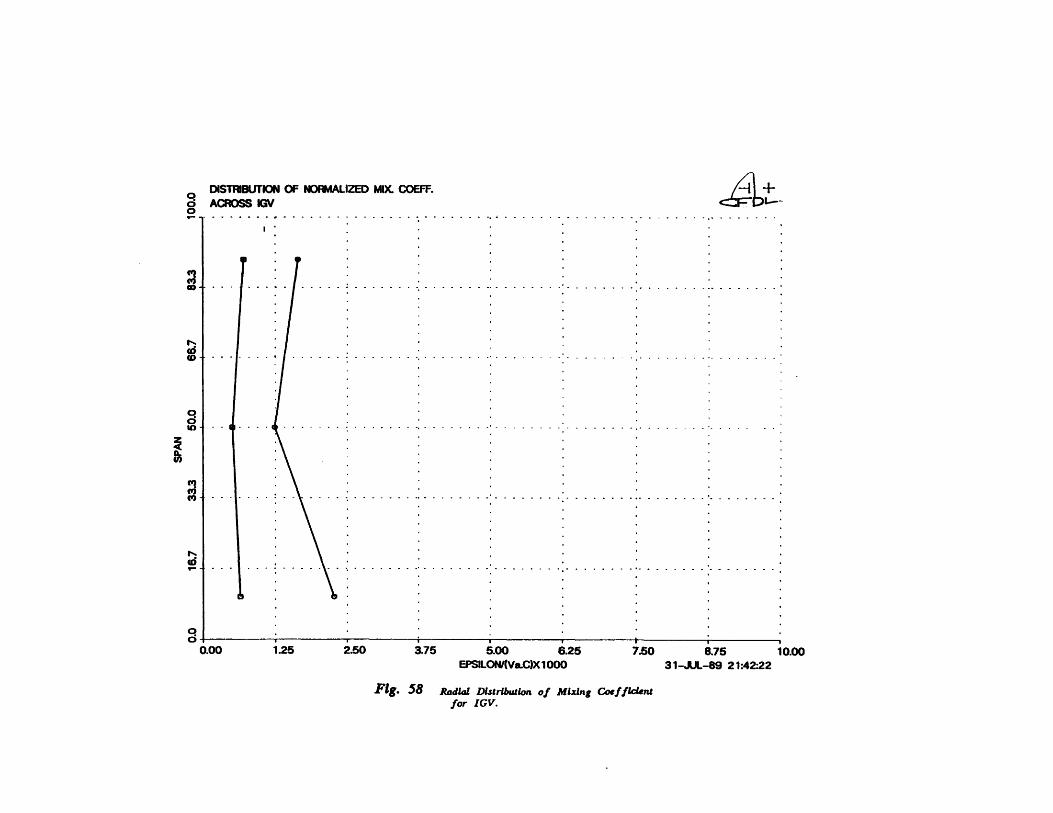
OF NORMALIZED MIX. COEFF.

5.00 6.25EPSILON/(Va.C)X1000

7.50 8.7531-JUL-89 21:42:22

FIg. 58 Radial Distribution of Mixing Coefficiedntfor IGV.

NDISTRIBUTIOIACROSS IGV

0.00 1.25 2.50 3.75 10.00LJ U B

-·

-

·

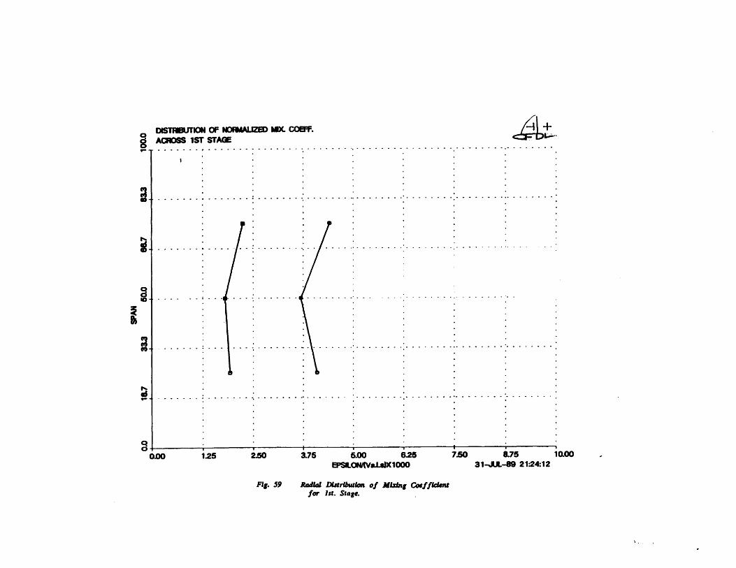
DIST•BUTMON OF NOUMALUD MX. COEF.ACOSS 1ST STAGE

6.00 6.25 7.50EPSILON4(Val.s)X1000

87531-JUL-89 21"24:12

Fig. 59 Radal DsnrlbuAon of Mlxing Coeffdientfor 1st. Stage.

0.00 1.25 3.75 10.00I r

250

1

-- · ·-- -:-·o ° o

. . . . . . . . .. . . ..

...............

. . . . . . . . . . . . . -. -

...............

...............·-

DISTFIBUTION OF NORMALIZED MIX. COEFF.ACROSS 2ND STAGE

125 2.50 3.75 5.00 6.25 7.50EPSILON/(Val.s)X1000

Fig. 60 Radial Distriftaon of Mixing Coeffldenfor 2nd. Stage.

8.7531-JUL-89 21"22:02

0.00 10.00

~b;t................ . . . . . . . . .

....... ...................

....... .................

.......... .. .........................

....... ....

. .. .......

DISTRIBUTION OF NORMALIZED MIX. COEFF.ACROSS 3RD STAGE

5.00 6.25EPSILON/(VaLs)X 1000

7.50 8.7531-JUL-89 21:18:42

Flg. 61 Radial Distribution of Mixing Coefficientfor 3rd. Stage.

0.00 1.25 2.50 3.75 10.00

· · · · ·

' '' '

- - - -- - -- - -- - --

. . .. . .. . .. .. . .

.. . .. . . - -- - -

.. . .. . .. .. .. . ..

. . .. . .. . ... . .. .

.. .. . .. . .. ..

.. . . . .. .. .. .

... .. . .. .. .

. . . .. .. .. . .

- - -- - -- -- --

. .. . .. .. .. .

"FF=:-...............

................

..........

...........

...............

...............

EVOLUTION OF MIXINGTHROUGH THE COMPRESSOR

dsign pointcreased loadingasign pointnoreased loading

For 11% turbulence

For 6% turbulence

1. 2. 3. 4. 5. 6. 7.BLADE ROW #

r-

0OOv.*

X

8

C0i

---------

. . . . . . .-• . . . . . . . . . . .- . . . . . . . . . ..-- - - - - --

, - - - - - - - - - - - - - - - - -

v

REFERENCES

1 Newton, A.G. "Shaping the Technology of Aircraft Propulsion",

Aeronautical Journal, January 1984.

2 Adkins, G.G. and Smith, L.H. "Spanwise Mixing in Axial Flow

Compressors", ASME 81-GT-57.

3 Gallimore, S.J. and Cumpsty, N.A. "Spanwise Mixing in Multistage Axial

Flow Compressors", ASME 86-GT-20.

4 Wennerstrom, A.J. "Low Aspect Ratio Axial Flow Compressors: Why and

What it Means", The Enginnering Society for Advancing Mobility, Land Sea

Air and Space, SAE/SP-86/683.

5 D.C. Wisler, et al. "Secondary Flow Turbulent Diffusion and Mixing in

Axial Flow Compressors", Journal of Turbomachinery, Oct 1987.

6 Y.S. Li and NA. Cumpsty "Mixing in Axial Flow Compressors",Unpublished Report, Whittle Lab., Cambridge University, England.

7 Kerrebrock, J.L. and Mikolajczk,A.A. "Intra-stator Transport of Wakes

and its Effect on Compressor Performance" ASME 70-GT-39.

8 Denton, J.D. and Usui, S. "Use of Tracer Gas Technique to Study Mixing

in a Low Speed Turbine", ASME 81-GT-86.

9 Towle, W.L. and Sherwood, T.K. "Eddy Diffusion, Mass Transfer in aPortion of Turbulent Air Stream", Journal of Industrial Engineering

Chemistry, 1939.

10 Hinze, J.O. "Turbulence", McGraw Hill Publ., 1959.

11 Moore, J. and Smith, B.L. "Flow in a Turbine Cascade Part 2:

Measurements of Flow Trajecteries by Ethylene Detection", ASME 83-GT-69

12 Abramovitz, GN., "The Theory of Turbulent Jets", MIT Press,Cambridge, Mass, 1963.

13 EM. Laws and J.L. Livesey, "Flow Through Screens" Ann. Rev. Fluid

Mech., 1978, 10:247-66.

14 Horlock, J.H. "Recent Developments in Secondary Flows", Secondary Flowsin Turbomachines, AGARD CP 214, 1977.

15 B. Cantwell and D. Coles "An Experimental Study of Entrainment and

Transport in the Turbulent Near Wake of a Circular Cylinder", J. ofFluid Mech. 1983, Vol. 136.

16 L.J.S. Bradbury " Measurements with a Pulsed-wire and Hot-wireAnemometer in the Highly Turbulent Wake of a Normal Flat Plate", J. ofFluid Mech. 1976, Vol. 77.

17 Townsend, A.A, "Turbulence", Cambridge Univ. Press, 1961.

18 Antonia, R.A. and Bilger, R.W. "Heated Round Jet in a CoflowingStream" AIAA, J 14, 1976.

19 Christianson, M.B. "An Experimental Investigation of a Three-stageAxial-flow Compressor with Cantilevered Stators Using Low Aspect Ratio- Redisigned Endwork Blading in All Stages" United Aircraft ResearchLaboratory Report *R232752-1, 1975.

10 Gamache, R.N., Ph.D. Thesis, MIT, "Axial Compressor Reversed FlowPerformance", 1985.

21 Lavrich, P.L, Ph.D. Thesis,MIT,"Time Resolved Measurements ofRotating Stall in Axial Flow Compresssor", 1988.

22 Bradshaw, P. "An Introduction to Turbulence and its Measurements",

Permagon Press, Oxford, England, 1971.

23 Feynman et al., "The Feynman Lecturs on Physics", Addison Publishing

Company, 1964.