Investigation of Spectral Baseline Properties of theGreen Bank Telescope

Electronics Division Internal Report No. 312

.1. R. Fisher, R. D. Norrod, D. S. Balser

September 2, 2003

Contents1 Introduction 2

1.1 System Description ........................................................................................................ 3

2 Antenna Noise 42.1 L-band (1.4 GHz) measurements ................................................................................ 42.2 C-band (5 GHz) measurements .........................................................................................92.3 X-band (9 GHz) measurements ................................................................................... 112.4 Antenna noise effects on observations............................................................................ 12

3 Antenna and receiver response to a continuum radio source 143.1 Quasi-periodic ripples in continuum source noise 143.2 Feed/LNA noise model.................................................................................................... 173.3 Fine scale structure due to cavity resonances ........................................................... 213.4 Continuum source spectrum stability .......................................................................... 253.5 Cal spectrum ripples ..................................................................................................... 30

4 IF system 324.1 2.4-MHz ripple from optical modulators .................................................................... 324.2 Baseline Periodicities Produced in the IF Electronics.................................................. 374.3 Changing Cable Lengths................................................................................................. 404.4 GBT Cables..................................................................................................................... 414.5 IF Converter Rack Ripple............................................................................................... 41

5 Spectrometers 465.1 Spectral processor wide-bandwidth distortions............................................................. 465.2 Autocorrelator linearity tests......................................................................................... 465.3 Offset problem in assembling composite receiver Tsrc/Tsys spectra ........................ 48

6 RFI................................................................................................................................. 49

7 Summary....................................................................................................................... 50

8 Attachments.................................................................................................................. 52

1

1 IntroductionOne of the primary motivations for the off-axis design of the Green Bank Telescope (GBT) wasto reduce the effects of multi-path interference, often referred to as standing waves, betweenthe feed, subreflector, and main reflector of the antenna. This interference causes low-levelripples in the frequency dependence of the gain of the antenna, which can mask weak spectrallines in the presence of continuum radiation from the spectral line source. Reflections in theantenna structure can also introduce frequency dependence of the total system noise which maynot completely cancel in on-source/off-source spectral differences or may show up as second-ordereffects in the calibration arithmetic. With an off-axis paraboloid the specular reflection areas thatcause the strongest gain and noise ripple are at the inner edge of the dish and subreflector wherefeed illumination is relatively low. Hence, the effects of these reflections should be correspondinglylower.

As will be shown in this report, reflections within the antenna are not the only source ofspectral baseline distortions. To realize the bill potential of the GBT design care must be takento minimize the effects of transmission line and waveguide reflections, amplifier and filter insta-bility, data sampling quantization, and other more subtle sources of spectrum distortion. Theinvestigation described here focused on separating the various effects as a guide to engineeringimprovements and calibration techniques that will follow.

Because of the claims of better baselines with an off-axis telescope it is natural to compareGBT results with spectra from symmetric antennas. Since we do not have much directly corre-sponding data from other telescopes, these comparisons must be largely anecdotal. In makingthese mental comparisons from your own experience keep in mind a few factors. First, thebandwidths of most of the spectra shown here are considerably wider than have been used atcentimeter wavelengths in the past. Second, the reflection distances in a 100-meter antennamakes the corresponding ripple periods of multi-path interference smaller than have been seenon smaller telescopes. Third, the spectra shown here were specifically designed to emphasizespectral baseline distortions so they are not necessarily representative of spectra that one wouldexperience under typical observing conditions.

Most of the spectra to follow are (on — of f)/of f vector differences and quotients, where thenormal assumptions are that the only difference between the on and of f spectra is the effectbeing measured and that the frequency dependence of the system gain is normalized by dividingby the system noise spectrum. Spectral baseline distortions are largely due to one or both ofthese assumptions being incorrect. Equation 1 is a partial separation of the gain and noise termsin the (on — of f)/of f vector, keeping the assumption that the only difference between the onand of f spectra is the injection of the continuum radio source power, 1?5.,(f).

- Off (1)off (f)Pbk,d(f) +

G2( f ) Pspii (f) + G3 ( (.f ) + PL N A (.f)

The noise spectra of the radio source, Ps, (f). background, Pund (f), and spillover, P5511 (f), areonly weakly frequency dependent., but the waveguide ohmic loss noise, P,„, (f), and amplifier noise,PLAT A(f). probably have a moderate to strong frequency dependence. Likewise, the gains of thesystem to the radio source and background noise, C ( f) and C 1 (f), are probably nearly equal,but the frequency dependence of the gains to spillover, G2

(f), waveguide, C3

(.f), and amplifier,

G :1(f ). noise are significantly different since they only partially share signal paths. Hence, theoff spectrum, which is the denominator of Equation 1, will not be simply proportional to thesystem gain to the radio source, G

STC(f)•

2

1.1 System DescriptionTypically, five to nine cryogenic receiver front-ends are installed on the GBT and available for use.All of the current front-ends are built around HFET amplifiers cooled to 15 Kelvin by closed-cyclerefrigerators, and depending on the frequency range, have one, two, or four feed horns. Eachfeed horn is followed by a dual-polarized receiver with two independent channels, so the existingfront-ends have two to eight channels. A common IF system has eight channels and microwaveswitches to handle the changes in connections required when a particular receiver is selectedand facilities to frequency convert the front-end signals to appropriate ranges for digitization.Figure 1 shows a very simplified block diagram of a receiver channel and critical portions of thecommon IF system. In this figure, components to the left of the fiber are located on the GBTfeed arm; items to the right are located in the Equipment Room in the Jansky Lab. Following isa brief description of each component of this diagram.

Feed Horn Above 600MHz all the GBT feed horns are circular corrugated horns. Below 4GHzthese feeds are fabricated using a "hoop-and-washer" technique. The corrugations areformed by stacking hoops and washers under pressure and then spot-welds are used to holdthe assembly together followed by the addition of a fiberglass shell for stiffness. Above 4GHzthe feed horns are machined from aluminum in sections eight to ten inches long containingseveral corrugations per section.

Front-end Electronics Following the cryogenic amplifiers, each channel is frequency convertedto a first IF center frequency of 1080, 3000, or 6000MHz. The first LO (L01) is used fordoppler tracking and frequency switching if desired. The mixer is followed by IF amplifiersand filters.

IF Router The switch symbol between the front-end and the Optical Driver Module in Figure 1represents a group of microwave PIN diode switches that select one of several possible inputsto each common IF channel.

Noise Source The IF Rack Noise Source consists of a solid-state diode noise source, amplifier,and filters and may be selected by the IF Router as an input to any of the eight OpticalDriver Modules. The Noise Source Module includes a four-way splitter that allows thesource to drive four IF channels simultaneously.

Optical Driver The Optical Driver Module (ODM) includes amplifiers, a filter bank for selec-tion of the IF bandwidth, an equalizer, and a total-power detector and V/F converter withfiber connection (not shown) to the Digital Continuum Back-End (DC13). The ODM's cover1-8GHz, but the user may select one of several more narrow bandwidths centered at either3000 or 6000MHz.

Laser Modulator The ODNI IF coaxial output is connected to a Laser Modulator which inten-sity modulates a laser output connected to a single-mode optical fiber.

IF Fiber The IF single-mode optical fiber is approximately 2.3km long, connecting the feedarm Receiver Room to the Equipment. Room in the Jansky Lab. Fusion splices are usedthroughout to eliminate instabilities typically seen with fiber connectors.

Optical Receiver In the Optical Receiver Module, the laser signal is demodulated using a pho-todiode detector. A microwave amplifier and four-way power splitter follow the photodiodeproviding four identical outputs of the first IF signal in the Equipment Room.

3

CONVERTER MODULE

CONVERTER MODULE

CONVERTER MODULE

CONVERTER MODULE

FIBER

NOISESOURCEMODULE

OPTICAL LASERDRIVER MODULATOR

MODULE MODULE

Figure 1: A simplified block diagram of one GBT receiver channel and associated IF electronics.

Converter Module Each Optical Receiver output is connected to a Converter Module (CM)which uses a two-step conversion scheme to supply signals with high image rejection toany of several back-ends. The input 1-8GHz IF signal is up-converted to the 9.0-10.35GHzrange, and then down-converted to the 150-1600MHz range. The various CM outputsconnect to the IF input systems of the Spectral Processor, VLBI Data Acquisition Rack,Autocorrelation Spectrometer, or other back-ends.

2 Antenna Noise

2.1 L-band (1.4 GHz) measurementsEarly in our investigations we were puzzled by a baseline ripple in frequency-switched data near1.4 GHz with a ripple period of about 1.6 MHz. It evidently had something to do with the antennabecause the phase of the ripple changed with subreflector position, and the phase changed byhalf of a period with an 1/8-wavelength shift in the subreflector toward the main dish. Thisripple period showed up again in later total power measurements where the blank sky on andoff spectra differed only by a displacement of the subreflector.

Figure 2 shows 50-MHz bandwidth difference spectra near 1.4 GHz for the two linear receiverpolarizations at 1/8- and 1/4-wavelength subreflector displacements between the on and offspectra. Several notable features can be seen in these spectra. First, there are quasi-sinusoidalripples with periods of about 1.6 and 9 MHz. Second, the 1.6-MHz amplitude is strongest in the1/8-wavelength subreflector displacement spectra, and the 9-MHz amplitude is strongest in the

4

roo

4-4

0o

Offset Subreflector

1 390 1 400 1410 1 420 1430Frequency in MHz

Figure 2: Cold sky (on - off) / off spectra at an elevation of 80 degrees, where 'off is with thesubreflector in its nominal focus position and 'on' is with the subreflector displaced in the H-Ydirection (roughly toward the center of the main reflector). The red or darker curves are forreceiver channel X and the green, lighter curves are for channel Y. The top curves are with 1/8-wavelength (26.7mm) displacement and the bottom curves are with 1/4-wavelength (53.3mm)displacement. The bottom curves are offset by -0.02 in the vertical direction to separate theplots.

\s,vvy.40,4,e'r•

1/4-wavelength displacement spectra. Third, the 1.6-MHz ripple amplitude is highest in the Ylinear polarization whose E-vector is parallel of the plane of symmetry of the telescope.

The waviness in the spectra in Figure 2 is a frequency dependence in the noise power enteringthe receiver feed and has something to do with the position of the subreflector with respect tothe rest of the optics. Another clue to the origins of the spectral ripples can be found in Figure 3,which shows periodograms generated by taking the Fourier transform of the spectra in Figure 2after removing the R.FI and 1420.4—MHz radiation from Galactic hydrogen. The period of the1.6-MHz ripple is spread over a range of periods from about 1.3 to 1.8 MHz. If we assume thatthis ripple is due to multipath interference, the path length difference ranges from about 165to 220 meters (300 meters divided by the ripple period in MHz), which is roughly the range oftwice the distance from the Gregorian feed to the main reflector via the subreflector. The GBTreflector geometry is shown in Figure 4. This leads us to the conclusion that part of the noisein the telescope system (cosmic background, atmosphere, spillover, or receiver/waveguide noise)enters the receiver through two paths: directly and after emission or reflection from the feed areaand then scattered from the circumferential gaps between the surface panels. Since these gapsrun along lines of constant phase as seen from the feed, their scattered waves are coherent at thefeed. We expect the scattering to be strongest in the linear polarization perpendicular to thegap length (channel Y), which is what is observed. Also, since this multipath involves two extrareflections from the subreflector, the ripple amplitude measured with this techniques should hestrongest for odd multiples of 1/8-wavelength. This, too is consistent with the measurements.

The strongest periodogram features in Figure 3 at about 9 MHz period are suggestive of anmltipath distance difference of about 30 meters, which is twice the distance from the feed to the

5

I/8-Wavelength Subreflector Offset 1/4-Wavelength Subreflector Offset

(b)

0.2 0.4 0.6 0.8 0 0.2 0.4 0.6 0,8

Inverse Ripple Period in 1/MHz Inverse Ripple Period in 1/MHz

Figure 3: Averaged periodograms of several 1/8-wavelength displacement spectra like those inFigure 2. The red or darker lines are receiver channel X, and the green, lighter lines are channelY. The vertical scale is roughly the ripple rms amplitude in units of 0.001 of the system noisepower density (fraction of Tsys).

Table 1: Periodogram integrals in the inverse ripple period ranges of 0.6 to 0.84and 0.1 to 0.12 for the 1.4 GHz data.

Periodogram IntegralsElevation sec(z) Total Power 1.6-MHz(Y) 9-MHz(X) 9-MHz(Y)

80.0 1.02 1.00 4.59 4.09 5.5314.5 4.00 1.25 4.44 6.93 10.569.5 6.06 1.46 5.48 4.11 13.23

subreflector. (See Figure 4.) Some of the noise in the antenna system is returned directly to thefeed after one reflection off the subreflector. This is consistent with the 9-MHz ripple componentbeing strongest in the 1/4-wavelength subreflector offset spectra. There is a hint in Figure 3that this reflection is partially resolved into more than one path-length component, which willbe shown in more detail in measurements with wider bandwidths described below.

To determine whether the noise that is causing the 9- and 1.6-MHz ripples is entering thesystem in the vicinity of the main beam (cosmic background and atmosphere) we measured theripple amplitudes at three telescope elevations of 80, 14.5, and 9.5 degrees to vary the amountof atmospheric noise seen by the main beam and near sidelobes. These elevations correspond toair masses of 1, 4, and 6, which would add about 1.5, 6, and 9 Kelvins of noise to the system,respectively. Table 1 shows these measurement results, which are the periodogram integrals inthe inverse ripple period ranges of 0.6 to 0.84 and 0.1 to 0.12 (distance ranges of 87 to 123and 15 to 18 meters) as a function of telescope elevation. The integrals are corrected for risingsystem temperature with sec(z) so that the values are proportional to temperature, not the ratioto system noise power. The 1.6 - MHz ripple amplitude does not appear to be dependent on

6

SUBREFLECTOR

Figure 4: GBT reflector geometry. The distances from the feed phase center to the main reflectorvia the subreflector are 80.9 and 125.9 meters for the inner and outer edges, respectively. Thedistances to the inner and outer edges of the subreflector from the feed phase center are 15.9 and13.5 meters, respectively.

elevation so we tentatively conclude that the noise engaged in this multipath interference is notentering through the the forward direction of the GBT. Channel Y (polarization perpendicularto plane of symmetry) shows a strong elevation dependence in the 9-MHz ripple, but channelX does not. These measurements may be confused by the superposition of several multipathsthat are only partially resolved at the distance of 15 meters. The distance between the feed andsubreflector changes on the order of 15 centimeters due to focus tracking as the telescope movesfrom zenith to horizon so the multipath interference patterns are expected to change somewhat.

Noise components in the antenna system that are not expected to change significantly withtelescope elevation are due to thermal losses in the feed/OMT/LNA and rearward main reflectorspillover. Each of these is estimated to be about 5 K as seen by the LNA, but the edges ofthe feed and surrounding structure is bathed in noise at somewhat higher temperature due tospillover. The feed is designed to reject most of this noise, but it is there, nevertheless. It is thisoff-center spillover noise radiation that is reflected back into the GBT optics and interferes withthe directly-received spillover noise in the feed. Hence, when computing the return loss requiredto produce the ripple amplitude observed one may need to assume a somewhat higher reflectedspillover noise component. Without a physical optics analysis of the spillover radiation we canonly guess at the amplitude of this component, but some rough calculations are instructive.

To estimate the magnitude of the reflection coefficient from the panel gaps required to producethe measured 1.6-MHz ripple, let Po be the power directly entering the feed and PR be thecoherent power transmitted or reflected into the optics. Since we will be computing power ratioswe can normalize to an impedance of one ohm and take the electric field amplitudes as

VO =

PO,

VR =

PR (2)

Let L, in dB, be the return loss of the power, PR, scattered back into the feed, and let p bethe equivalent voltage reflection coefficient.

L = —10 logi o (p2) (3)

The measured relative powers at the peak and trough of the baseline ripple will then be

P+ (vo pyR)2 2pVR1 ± (4)Po V0 2 VO

and

Po vo 2( Vo — pi/R ) 2 2pVR

1

The relative peak-to-peak and rms ripple amplitudes will then be

Pp-p 4pI7u

Po Po 170

andPr, Pp_ p \/ p VR

Po 2-0 Po AC)

Let's assume that the noise due to ohmic losses in the feed and waveguide components istransmitted coherently in both (Erections, toward the LNA and toward the antenna reflectors.Assume, too, that its temperature is 5 K and that the system temperature is 20 K. In the notationof the equations above, Psvs = 4 Pp = 4 P0 and VR = Vo = /J). Then, from Equation 7

p = 2 V -172 PSP

s

S

(8)

From Figure 3a we see that the highest 1.6-MHz ripple component for the polarization per-pendicular to the circumferential panel gaps is about 0.001 X Psy, but this is twice the valueOf Pr„ Psys given in Equation 8 since two ripple patterns with a 1/2-wavelength shift weresubtracted. Hence,

p 212- x 0.0005 = 1.4 x 10-3 (9)

andL = 57dB (10)

For the linear polarization that is largely parallel to the panel gaps the highest rms ripple ampli-tude shown in Figure 3a is only about 0.0001 x P . which corresponds to a return loss of about77 dB. The return losses computed from the highest 9-MHz ripple amplitudes seen in Figure 31)are about 45 and 51 dB for the polarizations parallel and perpendicular to the telescope's planeof symmetry, respectively.

In a memo dated February 6, 2001 Norrod and Stennes report on reflectometry measurementsof the GBT through the L-hand feed. At the distance of the subreflector they measured returnlosses of about 57 and 60 dB for the linear polarizations parallel and perpendicular to the planeof symmetry, respectively. These values are 12 and 9 dB higher than derived in the calculationsabove, which would indicate that there is more noise being injected into the multipath interferencethan the 5 K assumed. This may argue that spillover has a significant role in producing the 9-MHz baseline ripple. The reflectornetry measurements resolved the returned power into two orthree components separated by as much as 1.6 meters in one-way distance. This and the partialresolution of the 0.1/MHz feature in the periodograms suggest that several reflections from thesubreflector are mixed together in the 9-MHz period baseline ripples.

At the distance range of the main reflector Norrod and Stennes measured a return loss lowerli mit of 83 dB for the perpendicular polarization, which is close to the value of 77 dB from theripple amplitude calculations. Unfortunately, they did not make a measurement in the polariza-tion parallel to the plane of symmetry, which, in retrospect, would make a better comparisonwith the 1.6-MHz ripple results.

(5)

(6)

(7)

8

Table 2: Periodogra.m integrals in the inverse ripple period ranges of 0.56 to 0.75and 0.095 to 0.115 for the 5-GHz data.

Periodogram IntegralsElevation sec(z) Total Power 1.6-MHz(Y) 9-MHz(X) 9-MHz(Y)

65 1.1 1.00 1.08 0.24 1.1611 5.2 1.32 0.42 0.65 0.726 9.6 1.65 0.83 0.95 1.18

2.2 C-band (5 GHz) measurementsFigure 5 shows wider, 200-MHz bandwidth spectra taken at 5 GHz with the same displacedsubreflector differencing technique used to generate the 50-MHz bandwidth spectra at 1.4 GHz inFigure 2. The Y channel, whose linear polarization is parallel to the telescope plane of symmetry,in Figure 5 again shows the stronger 9- and 1.6-MHz ripples. The periodograms of these spectraare shown in Figure 6. The highest ripple components in the periodograms have Prms 1 P„,values of about 0.0005 and 0.0001 (which are twice the actual values because of the subtractiontechnique) at inverse periods near 0.11 and 0.6/MHz, respectively. -Using the same assumptionsof Ps, = 4 Pi? = 4 P0 that we used at L-band and Equations 8 and 3 we compute return lossesof 63 and 77 dB, respectively, for channel Y. These losses are 18 and 26 dB higher than thecorresponding values found at 1.4 GHz.

The reflection from the subreflector that causes the 9-MHz ripple period is a combinationof an edge diffraction and a near-specular reflection from the area of the subreflector close tothe parent ellipsoid's primary axis where the surface is almost normal to the line of sight fromthe feed. The return loss from specular reflection is expected to change roughly as wavelengthsquared, or about 11 dB from 1.4 to 5 GHz. A more detailed physical optics computation wouldbe required to account for the full 18 dB difference.

The 26 dB difference in the panel gap return loss between the two frequencies is more compli-cated. One might expect the effective scattering area of the gaps to change roughly linearly withwavelength since the current interruption is in one dimension. This would suggest only a 5 dBdifference. We are left to speculate that the rest of the difference may be due to the fact that thegap reflections are more resolved in distance with the larger bandwidth used at 5 GHz (hence,the reflected power is spread over more components), and that the coherence of the reflectionsover the full circumferential gap extents may be partially reduced by optics misalignments, whichwould have a larger effect at the shorter wavelength. Part of the difference might also be at-tributed to lower subreflector diffraction at the higher frequency which would inject less spillovernoise into the multipath interference.

One notable feature of the periodogram in Figure 61-) is that the longer period ripple at aninverse period near 0.1/MHz has clearly been resolved into a number of components. Channel Yappears to have one strongest component which channel X does not.

Table 2 shows the results of integrating the reflected power over the two ranges of the peri-odograms that show strong ripple amplitudes. This time the 9-MHz ripple in channel X showsan increase in amplitude with decreasing telescope elevation. but the other two integral rangesdo not show this trend. In the 1.4-GHz data it was channel V that showed the increase in 9-MHz ripple amplitude at lower elevation. Tt seems likely that the changes in integrated rippleamplitudes are largely due to factors other than the amount of noise entering the system in theforward direction of the GBT.

9

04s41"/VA

Nywoo„v)44‘,14,

••-•

(b)

Offset Subreflect,or

4950 5000 5050 5100Frequency in MHz

Figure 5: Cold sky (on - off) / off spectra at an elevation of 65 degrees, where 'off is with thesubreflector in its nominal focus position and on is with the subreflector displaced in the +Ydirection. The red or darker curves are for receiver channel X and the green, lighter curves arefor channel Y. The top curves are with 1/8-wavelength (7.62mm) displacement and the bottomcurves are with 1/4-wavelength (15.2mm) displacement.

1/8—Wavelength Subreflector Offset 1/4—Wavelength Subreflector Offset

0.2 0.4 0.6 0.8 0.2 0.4 0.6 0.8

Inverse Ripple Period in 1/kHz Inverse Ripple Period in 1/MHz

Figure 6: Periodograms of the 1/8-wavelength (a) and 1/4-wavelength (h) displacement spectralike those in Figure 5. The red or darker lines are receiver channel X. and the green, lighter linesare channel Y. The vertical scale is roughly the ripple rms amplitude in units of 0.001 of thesystem noise power density (fraction of Tsys).

10

1/4—Wavelength Subreflector Offset

0.02 0.04 0.06 0.08 0.1 0.12

Inverse Ripple Period in 1/MHz

Figure 7: Periodogram of the 1/4-wavelength displacement spectra on cold sky at 9 GHz withan 800-MHz bandwidth. The vertical scale is roughly the ripple rms amplitude in units of 0.001of the system noise power density (fraction of Tsys).

2.3 X-band (9 GHz) measurements

The same displaced-subreflector measurements were made at 9 GHz with a spectrometer band-width of 800 MHz. At this frequency the 1.6-MHz ripple was too weak to make useful mea-surements, but the wider bandwidth provided very good resolution on the reflections at thedistance of the subreflector. Figure 7 shows the periodogram of the 1/4-wavelength displacement(on — of fl/off spectrum from circularly polarized channel X for ripple periods greater thanabout 8.2 MHz. Quite a few sharp features can he seen with this higher ripple period resolution.

Table 3 lists the periodogram features labeled in Figure 7 with their measured location andcorresponding ripple period and the path length difference required in multipath interference tocause that ripple period. Figure 8 shows the Gregorian suLreflector and feed geometry at theorientation that it has with the telescope pointed near the horizon. The X-band feed is shown atthe secondary focus used in the measurement of the periodogram of Figure 7. The L-band feedseems to shadow the X-band feed in this drawing, but this is only the appearance in profile. Fland F2 are the prime and secondary focus locations, respectively. Ray path F2-A-OA goes to thefar edge of the main reflector. and F2-B-IB goes to the edge of the main reflector nearest the axisof the parent paraboloid. Lines B-OB and A-IA are parallel to the F2-A-OA and F2-B-IB rays.The lateral displacement of the subreflector in making these ripple measurements was roughlyalong the direction of a 45-degree angle down and to the left in this figure. F2 is in the planeof the Receiver Room roof. The distance F2-B is 15.9 meters, F2-A is 13.5 meters, and theL-. S-, and C-band feeds extend about 1.4, 0.9, and 0.9 meters above the Receiver Room roof.respectively.

Periodogram features L. K. and J are almost certainly (Inc to reflections from the ReceiverRoom roof and the tops of the L-. S-, and C-band feeds sending a small portion of the antenna.noise signal on an extra path distance to subreflector edge B and back. Periodogram features Ethrough H could be due to reflections off the structure of the prime focus receiver boom locatedto the top left of Figure 8. Spillover noise in a given direction could interfere with itself and cause

11

Table 3: Tentative identifications of multipath interference features in the periodogram ofFigure 7. See Figure 8 for subreflector/feed geometry references.

Inverse Path LengthPeriod Period Did from

Feature ( MHz -1 ) MHz Period (m) Remarks or possible causeA 0.0175 57 5.25B 0.0200 50 6.00 interf. of rays IA-A-F2 (gr, IB-B-F2 ??C 0.0250 40 7.49D 0.0350 28.6 10.49E 0.0525 19.0 15.74F 0.0688 14.5 20.61G 0.0850 11.8 25.48H 0.0925 10.8 27.73J 0.0975 10.3 29.23 S.R. edge B to L-band feed (29.0m)K 0.1000 10.0 29.98 S.R. edge B to S or C-band feed (30.0m)I. 0.1062 9.4 31.85 S.R. edge B to rcyr room roof (31.8m)

baseline ripple, if it has two ray paths to the feed. For example, spillover noise from the inneredge of the dish enters most strongly through ray path IB-B-F2, but it can also scatter fromsubreflector edge A and enter through path IA-A-F2. The difference in these two path lengths isabout 5.9 meters, which might account for periodogram feature B. Positive identification of allof the observed ripple periods would require further measurements. Whatever the explanations,most of these features must depend on changes in relative lengths of interfering paths withsubreflector displacement.. All of the peaks in Figure 7 are stronger with a 1/4-wavelengthsubreflector displacement than with an 1/8-wavelength displacement.

2.4 Antenna noise effects on observations

In total power. position switching observations. where the on and off positions are taken bytracking the antenna over the same hour angle or elevation track, the antenna noise ripples shouldcancel in the on f difference spectrum. Changes in antenna elevation will cause both changesin the amount of antenna noise due to the atmosphere and spillover and the geometry of thetelescope due to gravitational deformations and compensating focus tracking of the subreflector.Both of these will affect the antenna noise ripple pattern. If on - off are done by tilting thesubreflector or switching between two feed horns, then the antenna noise ripple cancellation willbe incomplete.

Frequency switching is much more problematic since the whole antenna noise ripple patternwill shift between the on and off spectra. If the frequency switching interval is equal to half ofone of the ripple characteristic periods its amplitude will be doubled in the on - of .f differencespectrum.

One might try intentionally displacing the subreflector or frequency switching by a full rippleperiod between the on and off or between two on. - off pairs in a way that cancels the antennanoise ripple. The problem with this is that it works well Rif only one period or usually onlyone multipath route. The panel gap reflections cause ripple periods from about 1.2 to 1.8 MHz,and these reflections arrive from different directions relative to any subreflector displacementaxis. The same period and direction of arrival spread is true for the longer ripple periods due tofeed area reflections. One also needs to be aware that the phases of the panel gap ripples move

12

Subreflector Geometry

A

—5 0 5 1 0

Distance in meters

Figure 8: Subreflector and Gregorian feed geometry with telescope pointed near horizon andX-band feed in position. B-TB and A-OA are ray lines to the edges of the main reflector.

twice as fast with subreflector displacement as do the ripples due to multipaths that involve onlyone additional subreflector reflection. A few simple experiments with subreflector displacementindicate that the limit on the amount of ripple amplitude reduction to be expected is on theorder of a factor of three and often considerably less. At a specific frequency and bandwidthone might be able to find a particular frequency switching subreflector displacement pattern thatdoes better. but it will require some experimentation. There may also be some merit in usinga much wider bandwidth than the astronomical spectrum requires to model the antenna noisebaseline ripples over the part of the spectrum without spectral lines in hopes that the model willprovide a good interpolation in the spectral line region of the spectrum.

A more subtle effect to watch out for is that the antenna noise portion of Ts s will have afrequency dependence. As mentioned in connection with Equation 1, this will show up in the(on — off) / off spectrum of a source with significant continuum radiation.

Finally, a rough estimate of the amplitude of the antenna noise ripple to be expected fromthe GBT ranges from about 5 to 40 mK rms at 1.4 GHz to about 2 to 8 mK at 9 GHz, with the

ripple being roughly three times stronger than the 1.6-MHz ripple. More detailed valuescan be found in the figures in this section. Careful total power, position switching can reducethese amplitudes by a factor of 30 or better.

One antenna noise source of baseline ripples that we did not investigate is the sun. Thisadds the additional parameter of the position of the sun with respect to the telescope pointingdirection, and it was more than we had time for in this investigation. It is certainly an aspect ofthe telescope that needs better quantification.

13

3 Antenna and receiver response to a continuum radiosource

For a good understanding of the spectral characteristics of the antenna, feed, and receiver front-ends of the GBT we need to separate the frequency dependencies of gain and noise power. Thesetwo quantities must then be characterized for different parts of the antenna/front-end systemto the extent possible. The previous section described the far-off-axis antenna gain effects onenvironmental noise power entering the system. This section deals with the main beam systemcharacteristics and the signal path through the feed and low-noise amplifiers.

There is no laboratory or absorber-type noise source that can be fed into the receiver or feedinput and assumed to be spectrally flat to the levels of interest to radio astronomy. Return-lossmismatches smaller than -60 dB can be significant, and it is impractical to construct test noisesources to this accuracy for the wide variety of receivers and test points in the GBT. Hence, weare left to tease apart the various gain and noise spectrum effects beginning with the assumptionthat the spectrum of a continuum noise source in the main beam of the telescope is smooth andvaries with a something like a simple power of frequency across the measured passband.

As was done in the investigation of antenna noise, the antenna optics geometry can be variedto uncover the effect of the antenna's gain on the radio source's signal. The major reflectorantenna gain effect that we expect is multipath interference, so the periodograms of on — offspectra are again useful.

For each receiver the antenna response to a continuum radio source was investigated byperforming on — off observations toward continuum sources with varying intensities. Typically,5-minutes were spent on and then 5-minutes off the continuum source. Figure 9 shows 200-MHz bandwidth observations toward the 5.7 -Ty continuum source 2232+1143 at S-hand (1990MHz). Three, 5-minute on — off pairs have been averaged together. The secondary reflectorwas positioned at the nominal focus for both the on and off observations. Note the quasi-periodic, large scale ripple with a period of 100 MHz and an amplitude of — 3% of the systemtemperature. Similar baseline structures are observed in all the Gregorian receivers and will bediscussed below. Also present in the channel Y data is the 9-MHz ripple thought to be caused byreflections from the sub-reflector and Gregorian feeds and the 1.6-MHz ripple caused by reflectionsfrom circumferential gaps between surface panels.

A new feature at 0.435 il/Hz. -1 (1/2.3 MHz) is also visible in both X and Y channels ofthe on — off spectra. This ripple is clearly detected in the periodogram shown in Figure 10.This frequency is close to the 2.4-MHz ripple detected from the optical fiber modulators (seeSection 4.1). However, the ripple phase changes by half of a period when the sub-reflector isshifted by A/4. indicating a single reflection involving the sub-reflector. The 2.3-MHz rippleperiod corresponds to a one-way distance of — 65 meters which is the distance between the sub-reflector and the primary reflector near the axis of the parent paraboloid (see Figure 4). Thisripple has also been detected at L-band (1400 MHz) and C-band (5000 MHz). The relative powerof the ripple increases as V.

3.1 Quasi-periodic ripples in continuum source noiseWhen observing strong continuum sources with the GRT Gregorian receivers, quasi-periodicripples are detected that appear to reside upstream of the first LO mixer and downstream of theoptics. The phase of the ripples are fixed to sky frequency and do not change when the opticalelements are adjusted; thus these features appear to reside in the feed, waveguide componentsand UNA. components.

Figure 11 plots on — of f spectra for three continuum n sources at L-band. Because of significantRFT only 50-MHz bandwidths were used. Two curves are shown for each source corresponding to

14

c.oCO I

cP900 1950 20502000Frequency in MHz

['V

I

0.4 0.5 0.6 0.7Inverse Ripple Period in 1/MHz

o

Continuum Source 2232+1143

Figure 9: (on - off) / off spectra toward the continuum source 2232+1143, centered at a skyfrequency of 1990 MHz. Three on — off pairs have been averaged. The red or darker curveis for receiver channel X and the green, lighter curve is for channel Y. The channel Y data havebeen offset by —0.1. The spectra have been smoothed by truncating the autocorrelation functionsto 2048 lags and Harming convolved.

Periodogram of Continuum Source 2232+1143

Figure 10: Periodograms of the spectra in Figure 9. The red or darker line is receiver channelX. and the green. lighter line is channel Y. The spike at 0.435 MHz -1 corresponds to a rippleperiod of 2.3 MHz and a one-way reflection distance of 65 meters.

14201410t

1380 1390 1400Frequency in MHz

Continuum Sources (2316+0405, 0054-0333, 0120-1520)

Figure 11: (on - off) / off spectra toward the continuum source 2316+0405 (4.68 Jy, red andorange curves in the middle), 0054-0333 (2.21 Jy. dark blue and blue-green curves at the bottom),and 0120-1520 (5.08 Jy, green and green-cyan at the top). The intensity scale of 0054-0333 arid0120-1520 were scaled by 1.9 and 0.98, respectively to put their spectra close to that of thefirst source, 2316+0405. for easy comparison. All spectra have been smoothed by truncating theautocorrelation functions to 4096 lags and Harming convolved.

Table 4: Front-end Ripple Periods.

Receiver BandS CX

Frequency (GHz) 1.4 2 5 9Ripple Period (MHz) 30 100 65

center frequencies of 1395 and 1405 MHz. Note the 30-MHz ripple in all spectra that are fixedin sky frequency and closely scale with source continuum intensity. Larger bandwidths can besynthesized by concatenating several 50-MHz pass-bands. Figure 12 illustrates such a compositespectrum toward 2316+0405 that spans 190 MHz. Each 50-MHz pass-band has been overlappedby 10 MHz. Unless the system temperature has significantly changed between successive spectrait is puzzling why the spectra do not match up in the overlapped region (this is discussed in moredetail below). The vertical lines correspond to BPI. There is a hint of a — 85-MHz ripple in thesespectra.

At S-hand (1990 MHz) a wider bandwidth of 200-MHz can be used. Figure 9 shows on — offspectra toward 2232 + 1143 as discussed above. The largest wavelength ripple detected is at — 100MHz. These features are fixed to sky frequency. they do not involve multi-path reflections fromthe telescope structure, and the results are generally repeatable.

Similar observations were made at C-band (5000 MHz) and X-band (9000 MHz) using thelargest available Spectrometer bandwidth of 800-MHz. These receivers also have large-scalespectral baseline structure that appears to be located in the front-end. The character of the

16

Continuum Source 2316+0405

1350 1400 1450 1500Frequency in MHz

Figure 12: (on - off) / off composite spectra toward the continuum source 2316+0405 that hasa flux density of 4.68 .1y at a frequency of 1400 MHz. The red or darker line is receiver channelX, and the green, lighter line is channel Y. The spectra have been corrected for a source spectralindex of —1.006 derived from the NVSS (Condon et al, 1998, A,I, 115, 1693) ,flux densities at1.4 and 5 GHz.

baseline structure is somewhat different, however. Figure 13 shows on — of f spectra toward0137+3309 at C-band. A 65-MHz ripple is clearly present with an amplitude of a few percentof the total system temperature. The baseline structure appears more sinusoidal than the L orS-hand structure. Additional investigation has revealed that these smooth features were at leastin part due to water on the S-hand feed. In contrast, the results of on — off spectra toward3C48 at X-band appears less sinusoidal (see Figure 14). The baseline structure is irregularwith very sharp features. The character of these X-band spectra is not consistent with typicalreflections between different front-end components (e.g., the feed and waveguide window). Suchbaseline structure has been observed before whereby weak cavity resonances are formed in thedewar resulting in significant structure in system temperature spectra. Possible locations forthis radiation are irregularities in the waveguide joints or the thermal gap located in the dewar.Copper tape placed around the waveguide joints near the feed throat had essentially no effect onthe baseline structure. Further investigation of the sharp features in the X-band spectrum aredescribed in Section 3.3.

Each receiver appears to have unique baseline structure that is located in the front-end com-ponents. This has been confirmed by changing the first LO mixer and the telescope optics. Thephase of these structures is fixed to sky frequency and is not affected by sub-reflector motion. Insome cases the baseline structure appears quasi-sinusoidal, suggesting reflections between variouscomponents in the front-end such as the LNA. OMT, or feed horn. Table 4 summarizes the mainripple frequencies observed for each receiver band.

3.2 Feed/LNA noise modelWe know that there are reflections within the feed and waveguide system of the GBT receiversdue to small impedance mismatches with return losses in the -30 to -60 dI3 range. Also, the

17

4800 5000 5200Frequency in MHz

Continuum Source 0137+3309

Figure 13: (on - off) / off spectra toward the continuum source 0137+3309 that has a flux densityof 6.6 .Ty at a frequency of 5000 MHz. The red or darker line is receiver channel X, and the green,lighter line is channel Y. The spectra have been corrected for a source spectral index of —0.81derived from the NVSS flux densities at 1.4 and 5 GHz.

Continuum Source 3C48

474-0

8700 8800 8900 9000 9100 9200 9300Frequency in MHz

Figure 14: (on - off) / off spectra toward the continuum source 3C48 that has a flux density of3.1 .Ty at a frequency of 9000 MHz. The red or darker line is receiver channel X, and the green;lighter line is channel Y. The channel Y data have been offset by —0.022 for clarity. The spectrahave been corrected for a source spectral index of —0.9 derived from Ott et al, 1994, AtVil, 284,331

18

optimum noise impedance of the LNA's is often at a point where its input return loss is on theorder of -10 to -20 dB. These reflections can cause gain ripples in the feed and waveguide systemin the same way as multipath interference in the antenna system.

We know, too, that noise is generated in the waveguide components due to ohmic losses and inthe LNA input stage. These noise sources transmit coherently in both directions, in the intendedsignal flow direction toward later receiver stages and toward the feed aperture and reflectorantenna. The backward-traveling noise components can be reflected by the small mismatchesand returned to the LNA input where they interfere with their forward-traveling components.Again, the extra path length of the backward-traveling power introduces a ripple on the noisespectra. If more than one reflection and path length are significant, the spectrum can be fairlycomplex.

Figure 15 is a schematic representation of a receiver feed and waveguide system. Equations 3and 6 can be used to compute the expected peak-to-peak ripple amplitude from a given reflectionreturn loss in the feed-waveguide system by setting VI? = Vo and Po equal to the noise componenttemperature. With 5 K of thermal noise traveling in both directions in the waveguide and returnlosses of 30, 40, and 60 dB, the peak-to-peak ripples will be 0.63, 0.2, and 0.02 K, respectively. Ifwe assume a 20 K system temperature, these numbers would represent a peak-to-peak variationin system temperature ranging from 3.2 to 0.1%.

Noise from the LNA input stage is a bit more complicated because VR, 170 , but the ratio ofthese two values is probably less than two, so the ripple amplitude from this source and the waveguide reflections should be comparable to or somewhat less than those of the ohmic loss noisesources.

Noise from the antenna (continuum radio source, cosmic background, atmosphere, and spillover)will also be modified by reflections in the LNA-waveguide-feed structure. Because this begins asforward-traveling noise the effective return loss to use in Equations 3 and 6 is the sum of thereturn loss that reverses its direction (typically at the LNA input) and the return loss where itis reflected to the forward direction again. If we assume a total antenna noise temperature of10 K and an LNA return loss of 10 dB, then the expected peak-to-peak ripple amplitude fromwaveguide return losses of 30, 40, and 60 dB will be 0.4, 0.13, and 0.013 K, respectively. With a20 K system temperature, these number correspond to a peak-to-peak variation in system tem-perature ranging from 2 to 0.06%. A radio source with a 10 K antenna temperature would havea peak-to-peak variation in its receiver power ranging from 4 to 0.13%.

The period of the noise spectrum ripples (Inc to waveguide and feed reflections will dependon the effective distance between the noise sources and reflections or between two reflections.The longest component in the system is generally the feed. Table 5 lists the lengths of the GBTfeeds and the corresponding ripple periods assuming a wave velocity equal to the speed of light.The total effective signal path length through the waveguide and coax line to the LNA maybe on the order of 50% longer, and the ripple periods may be scaled down by about 30%. Thelargest reflections at the LNA. OMT. waveguide window, and feed throat are separated by smallerdistances than the feed length so the highest ripple amplitudes would be expected at somewhatlonger ripple periods.

— Tentative conclusion: From the ripple amplitude calculations above and the ripple periodsgiven in Table 5 it seems unlikely that most of the observed variation in ITsrc, -sys, such as inFigures 9. 12, 13. and 14. can be explained by feed-waveguide-LNA reflections alone. For a moredetailed analysis of the noise and reflection properties of the system shown in Figure 15 see theattached memos by B. F. Bradley (January 30, 2003) and M. W. Pospieszalski (January 28,2003).

19

10K

Feed

WG

window

300K

LNA Gap

-10 dB —35 dB —35 dB —40 dB 50 dB

Dewar

up to 3.3 meters

2K 1 K 3K 1K

Figure 15: GBT receiver feed-waveguide-LNA diagram. Thermal noise sources and reflectionpoints are labeled with typical temperatures and return losses, respectively.

Table 5: Feed lengths and corresponding ripple periods implied byreflections at this distance.

Receiver Band

Frequency (GHz)Feed Length (m)Ripple Period (MHz)

L S C X Ku K1.4 2 5 9 14 203.3 2.2 1.2 0.56 0.37 0.2545 68 125 268 405 600

20

00 200 300 400 500 600 700

Frequency [MHz]

0

3048 [red] 3C123 [blue]

Figure 16: The normalized antenna temperature toward 3C48 (red) and 3C123 (blue). Eachspectrum consists of one 5 minute on-off pair. The antenna temperature, in units of the systemtemperature, were divided by the median value in the spectrum. The spectra are centered at asky frequency of 9000 MHz.

3.3 Fine scale structure due to cavity resonancesThe baselines when observing strong continuum sources with the GBT tend to show objectionablestructure, as mentioned elsewhere in this report. The X-band (8-10GHz) receiver in particularexhibited a great deal of relatively fine-grain structure that makes even narrow-band observationsdifficult.

Figure 14 shows the results of two 5 minute, on-off pair observations toward 3C48 (3.4 Jyat 8000 MHz). The very irregular structure is similar to what was reported earlier and appearsin both polarizations. The amplitude of these features scales with source continuum intensity.Figure 16 show the normalized antenna temperature for 3C48 and 3C123 (10.6 .Ty at 9000 MHz).The baseline structure is very similar.

These baseline features appear to be upstream of the first mixer. Figure 17 shows the antennatemperature versus sky frequency for two spectra centered at a sky frequency of 9000 MHz and9010 MHz. Notice that most of the baseline structure is fixed with sky frequency. Similar toother Gregorian receivers there appears to be broad band frequency structure which is upstreamof the first mixer but not related to the optics.

Independent analysis by Marian Pospieszalski and Richard Bradley showed that reflectionsbetween the cryogenic LNA (which has quite poor input return loss when matched for optimumnoise), and other input components such as the feed horn aperture, can introduce ripple in thereceiver noise. As shown earlier, the (on — of f)/of f data processing causes any non-uniformreceiver noise spectrum (as opposed to gain ripples) to show in the baseline spectrum. However,

I ■ I ■ 1 I I I

1

21

3048

87 100 8800 8900 9000 9100 9200 9300

Sky Frequency [MHz]3048

O

8900 8920 8940 8960 8980 9000

Sky F ,ecde-cy [MHz]

Figure 17: The antenna temperature toward 3C48, in units of the system temperature, centeredat a sky frequency of 9000 MHz (red) and 9010 MHz (blue). The lower panel shows an expandedview.

22

the LNA-Feed Horn reflection should be quite well-defined and dependent on the path length.which does not fit the observed characteristics.

Figure 15 shows in some detail a typical GBT front-end in the area between the feed hornand the LNA. The circular waveguide throat section of the feed horn connects through a low-lossvacuum window to a thermal transition assembly, which provides high thermal impedance bya small gap in the circular waveguide wall, and thereby allows the following components to becooled to cryogenic temperatures. Following the gap is a polarizer or 01\4T to separate the twopolarizations, and then each channel connects to a LNA. Not shown are stripline cal couplersbetween the OMT and the LNA: some receivers also have cooled isolators before the LNA. Dueto circumstances, the Ku-band (12-15.4GHz) front-end was first investigated in depth. to try tounderstand the baselines evidently due to fine-grain receiver noise structure. This receiver wasplaced in the Equipment Room and connected directly into two of the Converter Modules.

The Ku-hand receiver is one that has cooled isolators in front of the LNA's. so a tight waveg-uide short over the dewar input waveguide acts like a cold load of about 20K (the isolator loadphysical temperature, plus the effective temperature of any input losses). Figure 18 shows thetotal power spectra for the receiver with the thermal gap as normal, and with the gap temporar-ily covered with copper tape. Based on these results, it is likely that the several large noisespikes seen in the normal state are due to resonances or leakage related to the thermal gap. Thisconclusion was strengthened by S. Srikanth using the EM modeling program Quickwave. TheKu-band thermal gap uses a simple choke ring to provide RF isolation, and A. Kerr suggested analternative broadband choke design. A new gap using Kerr's suggestion has been designed andis now in fabrication to be evaluated.

Since the X-band baselines on continuum sources seemed to be particularly bad. when thetelescope schedule allowed this front-end was removed and brought to the Equipment Room forsimilar testing. A shorting plate was placed over the input waveguide. The total power spectrumshowed one spike near 9.7GHz that seemed similar to those seen in the Ku-band total power andwere identified with the thermal gap. Nothing was seen that obviously would cause the structureseen in Figures 14, 16, and 17. In order to simulate a continuum source observation, we decided totry using the internal calibration noise sources. While the noise cal is injected after the polarize'',part of the injected noise will be reflected off the LNA isolators, travel back to the waveguideshort, and back into the receiver. This excess noise should show the frequency structure seen onthe telescope, if it is generated in the receiver. For this receiver the low cal is about 2.5K andthe high cal is 15-30K.

A series of scans were taken while manually controlling the receiver noise sources. During thefirst scan pair, both the low cal and the high cal sources were off. During the second pair, thelow cal was on. During the third pair, the high cal was on. During the fourth and final pair,both cals were again off. Figure 19 shows the resulting scan ratios for the LCP channel for thissequence of scans; the RCP channel results are similar. While there is large ripple when scanpairs with the noise sources on and off are ratioed (expected because of the standing wave dueto the waveguide short), there is little evidence of extremely sharp frequency structure like thatseen on the antenna.

The negative result led to a close inspection of the feed horn assembly. Several quality issueswere identified with the assembly:

• One joint in circular waveguide between the feed horn and the vacuum window was foundto have a mistake that resulted in a 0.015 inch gap in the waveguide wall. The joint wasre-machined.

• Several (10-12) metal chips were found in the feed horn corrugations. These were evidentlyleft from the feed fabrication process.

23

100 200 300 400 500 600 700

Ku L1 by 700MHz, 2/10/03

400 500 600 700100 200 300

Freq,ncy [MHz]Ku Li, 3/3/03, CuTape on Gap ID

F ,eque ,cy [MHz]

Figure 18: The total power spectra of the Ku-hand receiver with a shorting plate over the dewarinput waveguide. Each panel covers 11.7 (lower left) to 15.2 (upper right) GHz. by five tracesoffset vertically for clarity and in frequency by 700MHz. The upper panel has the waveguidethermal gap as normal; the lower panel has the gap temporarily covered by copper tape.

24

• The chromate surface finish on the aluminum feed horn is generally non-conductive, and webecame concerned that this thin dielectric layer on the flange faces could be a detrimentalfactor. Hence, we mechanically removed the chromate coating from all the joint flangefaces. (The horn is fabricated in four sections with bolted joints.)

• A second wa.veguide joint had a noticeable oily film between the flanges. An investigationconcluded this was cutting oil from the installation of some helicoil threads when the receiverwas off in December 2002, and obviously the joint was not properly cleaned.

After these items were corrected, the front-end was reinstalled and observations of continuumsources repeated to evaluate possible changes in the performance.

Figure 20 shows the results of an on-off observation of 3C218: compare with Figure 14,on 3C48. The vertical ranges of these two figures are the same, as a fraction of the sourcetemperatures. The baselines after the lab work, while certainly not flat, are significantly smootherthan earlier ones. Note also that there is little commonality between the spectra of the twopolarizations, unlike what was seen before correcting the feed and waveguide defects. The mostlikely explanation for the improvement in continuum source baselines is that the clean-up of thewaveguide joints eliminated highly irregular losses at these joints (or one could think of it as noisewith lots of frequency structure leaking into the receiver). The (on —off)/olf calibration causesany irregularities (even at the fractional kelvin level is significant) in the system noise to appearin the baseline response. Since it is almost impossible to measure feed horn loss with the degreeof precision needed to see these effects, there is no substitute for extreme care in fabrication,quality control, cleanliness, and assembly of the receiver input waveguide and feed horn.

3.4 Continuum source spectrum stabilityOne of the results of this investigation will be to improve the noise spectrum characteristics of theGBT receivers with modifications to current receivers and design considerations in new receivers.However, it is not practical to eliminate all of the distortions to continuum source spectra so theremaining effects must be calibrated. The best calibration technique is to measure the systemresponse to a continuum source that is as much like the continuum source with expected spectralline radiation as possible, as is nicely described by Ghosh and Salter in the book "Single-DishRadio Astronomy: Techniques and Applications," ASP Conference Series, Vol. 278, p521. Sincethis generally requires moving the telescope to a different direction in the sky and involves a timedelay between calibration and observation of the source of interest, we need to know how farin time and angular distance one can carry the calibration. This section presents a number ofmeasurements that address these questions.

Figure 21 shows the result of using one continuum radio source to calibrate the spectrum ofanother one using the C-band (5 GHz) receiver with a 200-MHz spectrometer bandwidth. Theleft-hand panel of this figure shows the (on - off) / off or T/T spectra for NGC7027 forthe two receiver channels. In the central 90% of the passband the variation in source to systemtemperature ratio is on the order of 5% on a frequency scale of about 50 MHz. Much smallervariations can be seen at smaller frequency scales. The blip near 5100 MHz is probably EFL Theintegration time for each of the on and off spectra is five minutes.

The right-hand panel of Figure 21 shows the ratio of Ts,„/T spectra for 3C48 and NGC7027in the top red (dark) and green (light) curves. At this frequency the two sources have nearly thesame flux density so the values in the curves are close to one. Aside from a difference in spectralindex of the two continuum radio sources, the curve for receiver channel X is reasonably flat,which indicates that the continuum response of the receiver can be carried between two sourcesthat are at least 45 degrees apart in telescope elevation. 3C48 was at 76 degrees elevation and

25

Xband—LCP, Cals, TRXRDNO30605

I

1 00 200 300 400 500 600 700

Frequency [MHz]Xband—LCP, Cols, TRXR05030605

oiowoodhrtMoomw44,444440,*

,40,404,0N4.4,440**".444

100 200 300 400 500 600 700, ecuercy [MHz]

Figure 19: (on — of f)/off. for the X-band LCP channel with the input waveguide shorted, forvarious states of the receiver noise cal sources. Cases are: Cals Off for both scans (red): Low caloff for 'off and on for on (green); Low cal on for both (blue): Low cal on for 'off' and high calon for 'on' (cyan); high cal on for both (magenta): High cal on for 'off', and both cals off for 'on'(yellow); and both cals off for both 'off' and 'on' (orange - the top flat trace). The scan timeswere 300 seconds. The central portion of the upper panel is expanded in the lower panel.

26

3C218 3.14 Scan 5 3 levels

r"\\

o

. , . . . . . t

8600 8700 8800 8900 9000 9100 9200 9300

FresJency in MHz

Figure 20: (on — of f)/of f. for the X-band LCP (red) and RCP (green) channels, measuredon-off 3C218 after feed horn quality problems were corrected. Compare with Figure 14.

Continuum Source NGC7027 Measured Ratio 3C48 / NGC7027

(0)

4950 5000 5050 5100 4950 5000 5050 5100

Frequency in MHz Frequency in MHz

Figure 21: (on - off) / off spectra for NGC7027 (a) and the ratio of measured spectral powerdensities of 3C48 to NGC7027 (b) using a 200 MHz bandwidth. The vertical scale is the fractionof system noise power density. The red (dark) curve is for receiver channel X and the green(light) curve for channel Y. In panel (b) the top two spectra are ratio averages of (on - off) / offspectra: the middle two spectra are ratio averages of (on - off) raw spectra for same scan pairs:and the bottom two spectra are ratio averages of (on - off) raw spectra using a different scan pairfor NGC7027 with the bottom two plots offset vertically by -0.05 for clarity.

27

31-

0 0

0 co

510050504950 5000 5050 5100 4950 5000

(a) —a

°

0

0.3

Ratio of Successive Mesurements of NGC7027, Channel X Ratio of Successive Mesurements of NGC7027, Channel Y

Frequency in kHz Frequency in MHz

Figure 22: Ratio of NGC7027 continuum source (on - off) / off spectra at about 11-minuteintervals extending to 3 hours 5 minutes. Panel (a) is receiver channel X and (b) is channel Y.The top plot is the ratio of the spectrum from the second scan pair to the first pair. The nextplot down is the ratio of spectra for scan pairs 3 and 1, and so forth. The plots are assignedarbitrary offsets to create the time progression from top to bottom. The green plot at the bottomis a repeat of the first plot at the top for comparison of the first and last ratio spectrum.

NGC7027 at 31 degrees. The spectrum ratio for receiver channel Y varies by about 1% peak-to-peak on a scale of about 30 MHz. This ripple period is not characteristic of the discoveredantenna multipaths or any IF system reflections so it requires further investigation.

The lower two pairs of curves in Figure 21h show the ratios of spectral powers from 3C48and NGC7027 using only the (on — o ff) difference spectra rather than T.4r/T.s y s spectra. Theresults are essentially the same. This is a hit remarkable since Ts y s is expected to be a somewhathigher at lower elevation. The vertical offset of the top pair of curves from the middle pair is dueto this difference in Tsys at lower elevation for NGC7027, but the shape of the spectral powerratio appears to be unaffected. The receiver is sufficiently stable between the measurements ofthe two sources to permit the ratio of uncorrected spectrum values to be computed directly.

Figure 22 shows the results of a test of system stability of the two channels of the C-band (5GHz) receiver with a 200-MHz bandwidth over a three hour period. In this figure are plotted theratios of the (on - off) / off spectra of NGC7027 for the two receiver channels at 11-minute intervalsto the first (on - off) / off spectrum at the beginning of the three hours. The spectra for channelX show very little change over the three-hour period, but channel Y shows structure at roughly9- and 60-MHz ripple periods. These periods are characteristic of multipath interference fromreflection from the receiver room and IF system instabilities, respectively, as explained elsewherein this report. Even the ratio of the first two (on - off) / off spectra show these ripples so thesechanges happen on times scales of 10 minutes or less. Work is in progress to improve the IFstability, and the changes in the 9-1\111z ripple period from the optics needs further investigation.

One of the questions that needs to be answered in connection with continuum source responsecalibration is whether the telescope has a different response to an extended source than to a sourcethat is small compared to the beam size. Figure 23 shows a test to determine the telescoperesponse near the half-power points of the beam compared to the center of the beam. There is abit of structure in the ratios of the east and west offset spectra to the beam center spectrum, butgenerally the ratios are what is expected from the decrease in beam size with increasing frequency.

28

(NIS1 09)/Center (on — off) Ratio, Channel Y, 1042+1203

143014201390 1400 141043014201390 1400 1410

Frequency in MHz Frequency in MHz

(NISIEIW)/Center (on — off) Ratio, Channel X, 1042+1203

Figure 23: Ratios of (on - off) spectra of 1042+1203 taken with the telescope pointed about 4arcminutes off beam center and at the beam center. Panel (a) is for receiver channel X and panel(h) is for channel Y. The red, green, blue-green, and violet lines correspond to 4-arcminute north,south, east, and west beam offsets. The blue lines show the expected ratio slope due to changingbeam size with frequency.

However, the north and south offset spectrum ratios show a significant amount of ripple with aperiod of 2.3 MHz, which is the ripple period associated with the multipath reflection between theedges of the main reflector and subreflector nearest the axis of the parent paraboloid. ChannelY also shows some 9-MHz ripple associated with multipath reflections between the receiver roomroof and the subreflector.

The data displayed in Figure 23 were taken near the meridian so the north-south offsetswere nearly in the directions of increasing and decreasing elevation. Hence, the area around thespecular reflection from the two surfaces moved onto or off the edges of the two reflectors with thenorth and south offsets so one would expect the intensity of the multipath interference to changemost in these directions. If a reasonably symmetric extended source is centered in the beam onemight expect the ripples from the two offset direction to partially cancel, but these measurementsdo make the point that some caution moist be exercised when calibrating the telescope's responseto extended continuum sources.

Not all continuum source spectra were as stable as those shown in Figures 22 and 23, and eventhe best of these calibrated spectral baselines are not perfectly flat. More extensive measurementswith longer integration times need to be done in connection with specific astronomical problemsto more fully explore the limits of this calibration technique. We know, for example, that thegeometry of the GBI changes with elevation (Inc to gravitational deformations and intentionalmotion of the subreflector to track the best focus position. Hence, we expect the pattern ofthe multipath interference connected with optics reflections to change with telescope elevation.This is not evident in the 5-GHz data in Figure 22, but it can be seen in similar tests, shown inFigure 24. at 1.4 GHz where the reflections are generally stronger. During the two hours of thisscan series the radio source, 2316+0405, went from an elevation of 47 degrees to 27 degrees. Themain feature that appears after some time is the 2.3-MHz ripple period from the subreflector tomain reflector multipath. The wave in the middle spectrum of Figure 24b may have been causedby a drift in the electronics, but this remains to be tracked down.

Because of the vagaries of the weather and IF electronics baseline problems that tend to

29

(C)

4.4440440#004'14,400* NoOwe

IksIt'N'141040,0040k, 't**P4'SA0446,00,,,‘ 4,1e4,h4"0144.0 04'sieS1

NYY ‘1,,Y114‘%4

(on — off) Ratios of 2316+0405 Scan Pairs, Channel X (on — off) Ratios of 2316 + 0405 Scan Pairs, Channel Y

0.-C)

00,00 0

00°

o

'41 0

G4i

0444td0+4*

i *Aio44404

4:f*A0

V44

14

04444,44,,,,,,,o/sor"(

0/44e0YN"

siA4004#4„60 0"S004

0'00

4',04kokiNvki4

‘4

44,6o04

'IVO"

(b)

1390 1400 1410 1420 1430 1390 1400 1410 1420 1430

Frequency in MHz Frequency in MHz

Figure 24: Ratio of 2316+0405 continuum source (on - off) spectra at intervals of 23. 47. 70. 93.and 116 minutes. Panel (a) is receiver channel X and (b) is channel Y. The plots are assignedarbitrary offsets to create the time progression from top to bottom.

dominate the spectra using wide bandwidths we were linable to make a useful assessment ofcontinuum calibration stability in the higher frequency receivers. This is something that needsto be revisited after improvements have been made to the IF electronics.

3.5 Cal spectrum ripplesDuring most observations a calibration noise diode (CAL) injects noise into the system with aperiod on the order of a second. The goal is to provide a rough flux calibration and to removeelectronic drift. The CAL signal does contain frequency structure, however. and currently theintensity scale is only known to an accuracy of about 10% with a sampling in frequency of 1%of the front-end bandwidth. When spectra are generated using the CAL signal the frequencystructure from the CAL itself will be folded into the final spectrum. It is difficult to decouplefrequency structure arising from the CAL and other components generating system noise.

Examples of /Tal, — SN'S ratios are shown in Figure 25 toward cold sky at L (top left). S (topright). C (bottom left). and X-band (bottom right). Note that the bandwidth varies dependingon the frequency. Each of these plots can be compared to (on — of f)/of f spectra shown inSection 3.1. In general the spectral baseline structures are similar.

Although the CAL was firing during all of the observations discussed thus far, because boththe on and off phases are stored separately. the CAL can effectively be removed by only usingthe CAL off data when processing spectra (e.g.. producing (on — of f)/of f spectra). Figure 26shows on — off spectra toward 0137+3309 at C-band (5000 MHz) that have been producedusing both on and off CAL phases (panel a) and only the off CAL phase (panel b). Plotted inboth cases are (on — off) and (on — of Plof f spectra. General inspection of these plotsindicates that the baseline structure is not dominated by structure in the CAL as both figures arevery similar. The structure in the (on — off) spectra comes primarily from the gain frequencydependence (see Figure 27). This is typically why these data are divided by the off spectrum.Also plotted is the antenna temperature. Ta . in units of the CAL (effectively (on — of Plof f

ti mes the off system temperature evaluated per channel). This spectrum is noisier since we aredividing by a noisy Tca t spectrum.

30

20501420 1900 1950 2000Frequency in MHzCold Sky (X-band)

1390 1400 1410Frequency in MHzCold Sky (C-band)

4600 5200 4800 5000 5200Frequency in MHz

5000Frequency in MHz

`fon - off) / off

(b)

Continuum Source 0137+3309

(a)

(on - off)

Continuum Source 0137+3309 (CAL off phase only)

(on - off)

Cold Sky (L-band) Cold Sky (S-band)

4800 5000 5200 8700 8800 8900 9000 9100 9200 9300

Frequency in MHz Frequency in MHz

Figure 25: Tc . /alT

, sys ratios toward cold sky for L. S. C. and X-band. The red or darker line isreceiver channel X. and the green 1 lighter line is channel Y. The L and S-hand spectra have beensmoothed by truncating the autocorrelation functions to 2048 lags arid Harming convolved.

Figure 26: Total power spectra toward the continuum source 0137+3309 for channel X at C-band(5000 MHz). Panel (a): (on — off). (on — of f)/off. and the antenna temperature (Ta ) inunits of the CAL. For the on and off data the CAL phases have been averaged. The Ta spectrumhas been offset by —2.5 for clarity. Panel (h): (on — off) and (on — of PI of f where only theoff CAL phase has been used.

Pe.' 0

d

31

Cold Sky (C—band)

Pass—band Power

Teai/Tsys

CV

4800 5000 5200Frequency in MHz

Figure 27: Total power spectra toward cold sky at C-band (5000 MHz). Plotted in red or thedarker line is the pass-band power. Plotted in green or the lighter line is the Tcal asys ratio. Onlychannel X is shown.

4 IF system

4.1 2.4-MHz ripple from optical modulatorsThe GBT IF signal is routed from the front-end to the back-end via optical fiber. There is atotal of 8 optical driver modules (ODM's) located at the front-end and an equivalent number ofoptical receiver modules (ORM's) at the back-end.

Measurements of fiber transmission stability early in GBT construction showed that twist-ing or bending of the fiber changes the polarization of the laser light (which is almost linearlypolarized) at the detector end. Since all of the photodetectors are polarization sensitive (the"gain" depends on the light polarization). Hence, the polarization rotation gets converted to aamplitude modulation so the effective gain of the optical link is unstable. A servo system forstabilizing gain of the fiber link was developed which required the use of externally modulatedlasers whose intensity can be controlled through feedback of the detected optical power at thereceive end of the fiber.

Unfortunately. a 2.4- .N1Hz period gain ripple is produced by these external modulators. Fig-ure 28 plots the total power and the autocorrelation function for observations using the externalmodulator located in ODM 6. The IF noise source located in the IF rack at the GBT ReceiverRoom on the feed arm was used. The 2.4-MHz ripple is clear in both plots. The spike nearlag 667 corresponds to a ripple period of 2.3988 MHz. The spikes near lags 1333 and 1999 areharmonics and indicate that the ripple is riot purely sinusoidnl.

An approximate quantitative measure of the amplitude of the gain ripple relative to the totalnoise spectral density was computed by summing the three highest absolute values of the ACFnear each ACF ripple spike and taking its ratio to the zero-lag ACF value. Figure 29 plots theresults using only the fundamental. ODM's 1. 2. 3. 5. and 6 correspond to different externalmodulators. ODNI's 4 and 7 were out of service. ODM 8 used a direct modulator which isknown to not have any gain ripple: therefore it provides a measure of the detection limit of this

32

500 1000 1500 2000Lags

330 335'310 315 320 325Frequency in MHz

Pass-band of IF Noise Source (Original ODM 6) ACF of IF Nth se Source (Original ODM 6)

(a)

Figure 28: IF noise source spectra of an original external modulator. Panel (a): total powerpass-hand averaging over 60, 30-second records. Panel (h): the autocorrelation function.

algorithm. Three different IF frequencies were explored: 1500. 3000, and 6000 MHz. The spreadin ripple amplitude for the five external modulators is about 5 dB ; and the amplitude is about 8dB higher at an IF of 1500 MHz than at 6000 MHz. The first and second harmonics are about6 and 10 dB weaker than the fundamental.

The manufacturer has since modified the external modulators and claims to have reduced theamplitude of the gain ripple. Figure 30 summarizes the results of similar tests using the IF noisesource for the new unit. The 2.4-MHz ripple is now not visible in the total power spectrum. TheACF plot does reveal the fundamental and the first two harmonics, but the amplitude of the gainripple is down by — 17 dB. Figure 31 shows a comparison between the original and new externalmodulators.

Although the 2.4-MHz gain ripple has been significantly reduced it may appear above the noiselevel for very sensitive spectral line experiments. The ripple frequency of 2.4 MHz correspondsto 24 A km s' where A is the observing wavelength in centimeters. Unfortunately, this is similarto the line widths of many astronomical source transitions. (For example, at K-hand (1.5 cm)this corresponds to 36 km s -1 ). The magnitude of this problem will depend on the amplitude ofthe gain ripple in raw spectra and the stability of the ripple in time. If the gain ripple is verystable then it should cancel when processing the data.

Tests were performed to quantitatively measure the stability of the optical fiber ripple. Threedifferent ODM's were used consisting of an original external modulator, a new modified externalmodulator, and a direct modulator. The IF noise source was used to simulate 5 minute on — offtotal power pairs by calculating (on — of f)/off for consecutive groups of data records. A totalof 400, 30-second records (200 minutes) were generated with the IF noise source. The data weredivided into four groups of 100 records (50 minutes), each consisting of five on — off pairs.

Figures 32, 33, 34 summarize the results for the original external modulator, the new modifiedexternal modulator, and the direct modulator, respectively. For each plot the (on — off)/of fspectra are shown along with the periodogram. Notice that a — 60-MHz ripple is quite strongin some spectra and is related to other sections of the IF system (see Section 4.2). The 2.4-MHzripple is only detected for the original external modulator. In fact, additional averaging of thedata decreases the amplitude of the ripple for this unit. Based on these results, eight modifiedexternal modulators have been ordered.

33

62 3 4 5IF Center Frequency in GHz

2.4 MHz Ripple Amplitdue (Fundamental)

erv nf IV N • (N nnia a)

(b)

11 )

Figure 29: Approximate amplitude of fundamental periodicity component of the 2.4-MHz gainripple measured at IF center frequencies 1.5, 3.0, and 6.0 GHz. The amplitude is relative to thezero-lag ACF value. The red, green, dark-blue, blue-green, violet, and yellow lines correspond tofibers 1, 2, 3, 5, 6, and 8, respectively. ODM 8 uses a directly modulated laser, which is knownto not have any gain ripple.

Pass—band of IF Noise Source (New ODM 6)

(a)

310 315 320 325 330 335 500 1000 1500 2000Frequency in MHz Lags

Figure 30: IF noise source spectra of the new external modulator. Panel (a): total power pass-band averaging over 60, 30-second records. Panel (b): the autocorrelation function. Comparewith Figure 28

34

Frequency in MHz Inverse Ripple Period in 1/M1iz

Synthetic Spectra (Original External ODM) Periodogram (Original External ODM)

200 400 600 0.3 0.35 0.4 0.45 0.5

(a)

ACF of IF Noise Source

620 640 660 680 700 720Lags

Figure 31: Autocorrelation function of the IF noise source. The red or darker line is the result forthe original external modulator. while the green. or lighter line is the result for the new externalmodulator. A total of 60. 30-second records have been averaged.

Figure 32: Synthetic spectra using the IF noise source and an original externally modulated laser.Panel (a): (on - off) / off spectra using 5-minute scan lengths. Each spectrum consists of 5 pairs(50 minutes). Panel (h): Periodogram for each spectrum.

35

Synthetic Spectra (New External ODM) Periodogram (New External ODM)

200 400 600 0 3 0.35 0.4 0.45 0.5Frequency in MHs Mverse Ripple Period in 1/MHz

Figure 33: Synthetic spectra using the IF noise source and a new externally modulated laser.Panel (a): (on - off) / off spectra using 5-minute scan lengths. Each spectrum consists of 5 pairs(50 minutes). Panel (h): Periodogram for each spectrum.

Synthetic Spectra (Direct ODM) Periodogram (Direct ODM)

200 400 600 0 3 0.35 0.4 0.45 0.5Frequency in MHz Inverse Ripple Period in 11'MHz

Figure 34: Synthetic spectra using the IF noise source and a directly modulated laser. Panel(a): (on - off) / off spectra using 5-minute scan lengths. Each spectrum consists of 5 pairs (50minutes). Panel (h): Periodogram for each spectrum.

36

(a)

IF Noise Source Spectrum Difference over 5 Minutes

1300 900 1000 1100 1200 1300 1400 1500

Frequency M KHz

Periodogram of Unstable IF Spectrum

0.01 0.02 0.03 0.04 0.05 0.06Inverse Ripple Period al 1/xi004

Figure 35: Difference spectrum, (spectrum2 - spectruml) / spectrunil, of two 30-second integra-tions on the IF noise source taken 5 minutes apart (a) and its periodogram (b).

4.2 Baseline Periodicities Produced in the IF ElectronicsIn the process of disentangling the various baseline distortion effects we frequently saw a ripplewith a period in the range of 60 to 80 MHz when using the 800 MHz spectrometer bandwidth.The amplitude of this ripple varied irregularly on time scales of minutes ; and it was eventuallycorrelated with small temperature changes in the GBT control room where much of the IFelectronics is housed. As of this writing the major cause of the problem has been traced toelectronic components in one or two of the IF conversion and filter modules, but it appears thatthere is more than one temperature-sensitive component in the IF chain contributing to baselineinstability. Here is what we know thus far.

Figure 35a shows an example of an 800-MHz spectrum when the IF baseline instability isquite prominent. The noise power in this spectrum is from the IF noise source substituted for theGBT receiver's IF output in the GBT Receiver Room. The frequency scale in this figure refers tothe IF passband at the input to the spectrometer sampler. The periodogram of this spectrum isshown in Figure 35b. The most notable feature in the periodogram is the spike at 0.016 1111-1z-1(62-MHz ripple period), but there are other significant periodicities in this spectrum. The largestspike at 0.005 MHz (200-MHz ripple period) is hard to interpret since it is a substantialfraction of the total spectrum width.

The correlation of the amplitude of ripples, such as those in Figure 35, with GBT equipmentroom temperature can be illustrated by plotting the strength of the dominant spike in a spectrum'speriodogram as a function of time along with a plot of the measured temperatures in the room andin the rack containing many of the IF electronics modules. This is shown in Figure 36. There is aclear correlation of 62-MHz ripple amplitude with the temperature of the rack containing some ofthe IF electronics used in this measurement. However, the correlation between temperature andripple amplitude for other periods seen in the periodograms and between amplitudes of differentripple periods is not always obvious. This indicates that there is more than one cause of thebaseline instabilities in the IF system.

Figure 37 shows a summary of the various ripple periods found in the periodograms of(recordN - recordl) / recordl spectra over roughly a five-hour period, where recordN isthe Nth 30-second record in the run. The open boxes in this figure refer to periodogram fea-tures that occurred occasionally or weakly. and the filled boxes are for strong features that werepresent much of the time. Most of the IF channels showed a dominant ripple period around 0.016MHz- 1 (63 MHz). but there was significant variation in this period from channel to channel,and these periodogram features tended to be composed of several closely spaced periods whose

37

26

UTC in hours

t

27 2824 25

Comparison of Ripple Amplitude with Rack and Room Temperature

,r)a0no

-FJ

P

ut,0) 0

o-

Figure 36: Correlation of the 62-MHz ripple period amplitude in IF channel Al (top curve) withconverter rack A internal air temperature (middle) arid GBT equipment room air temperature(bottom). The temperature values have been multiplied by 0.2 and given an arbitrary zero offsetto allow easier visual comparison with the ripple amplitude curve.

amplitudes were not necessarily well correlated in time. Channels A2 and C2 were considerablymore stable than the others. Most channels had quite a variety of periodicities that came andwent with time with only partial correlation. This, too, indicates that there is more than onecause of baseline ripple in each IF channel.

The three rows at the bottom of Figure 37 are the equivalent periodogram distributions forthe spectra obtained by differencing spectra taken before and after intentional changes to IF cablelengths at three different places in the IF system. Figure 38 is a schematic diagram of the GBT IFsystem between the front-end and the spectrometer. There are four cables with lengths between2.4 and 7.1 meters between the different IF modules. As will be explained in the next section,if there are mismatches at the ends of these cables that cause part of the signal to traverse thelengths of the cables twice again, the multipath interference will cause frequency-dependent gainripples. Very small changes in the electrical lengths of these cables will cause the gain ripplesto change in phase, which can manifest themselves as temperature-dependent gain ripples in thesystem noise spectrum.

The gain ripple periods corresponding to the 2.4-, 6.5-, and 7.1-meter cable lengths are shownat the bottom of Figure 37 as measured with the cable length change experiment. There may bea strong effect associated with the 2.4-meter cable corresponding to a ripple near 0.016 MHz—I(63 MHz) as seen by the period correlation in Figure 37, but there are no periods evident inthe IF noise periodograrns corresponding to the other two cable lengths, even though one mightexpect a comparable or larger temperature sensitivity of the longer cables. As of this writing itis not clear how large a role the temperature dependence of the electrical lengths of these cablesplays in the observed IF baseline instability. It is likely that this effect is a significant problemso the procurement of more stable coax is under way.

38

1.5, 3, or 6 GllzReceiver

OpticalModulator

Notable Periodogram Features for Eight Channels

E

-5

-5

L-1)

c)

fa,C/)

- Al

-A2

- B1

- B2

Cl

- C2

-D1

- D2

OE •••

0 0 CI O

LEE ••CIO

•••0

CO••

COO a n 0

0 0 0•00000E • O nn

0

0000 CI00

000- 10 a C

-

00E0E-

000000 -

- 63

- 23

- 21

O 0 • • 0 0

• a n

• 0

0 0.01 0.02 0.03 0.04 0.05Inverse Ripple Period, 1/MHz

Figure 37: Ripple periods found in the periodograms of eight of the sixteen GBT IF channels forthe five-hour run used in Figure 36. The rows are for different IF channels labeled by spectrometeroutput channel. The bottom three rows show equivalent results for the FFT's of spectra obtainedby changing IF cable lengths as reported below. Rows "63" "23" and "21" refer to the 63-, 23-and 21-MHz ripple periods that are characteristic of the cable lengths given in Figure 38.

Optical Fiber

OpticalReceiver

1 08, 1.5, 3or 6 GHz

(2.4 rri

ConvertorModule

AnalogFilter

Module

SpectrometerSampler

0.8-1.6 GHz 0.8-1.6 GHz

Figure 38: Schematic diagram of one GBT IF channel. The figures in rounded rectangles arecable electrical length in meters, and above each is the frequency range carried by this cable whenusing the 800 MHz spectrometer bandwidth.

39

4.3 Changing Cable LengthsWe performed tests on the GBT Equipment Room IF electronics in an attempt to isolate thesource of near sinusoidal baseline ripples that show up from time-to-time. We injected a stablenoise source into Converter Modules or into Sampler/Filter Modules, and simulated positionswitched observations by running a series of scans using the spectrometer's 200-MHz bandwidth.During the course of these tests, we induced small changes in the length of coaxial cables connect-ing various pieces of equipment by inserting short coaxial adapters. This introduced dramaticripples in the baselines (Figure 39), calculated by the usual methods.

In order to understand this ripple-producing mechanism, it is helpful to revisit some two-portnetwork theory. Figure 40 shows a signal-flow representation of two two-port networks, Net Aand Net B, connected by a lossless, matched transmission line. The scattering parameters i i and8 22 are input and output reflection coefficients of the networks. Parameters 82 1 and 8 12 representthe forward and reverse transmission coefficients. The s-parameters are complex values that, ingeneral, vary with frequency. The delay of the lossless, matched transmission line is representedby a transmission coefficient in phasor notation: e 1 i31 , where /3 = 27/A and 1 is the electricallength of the transmission line. In Figure 40, complex voltage signals flowing toward the rightare represented by a, and signals flowing toward the left by hi.

We are interested in (Li /a i . The square of the magnitude of this quantity is the transducerpower gain of the cascaded networks. The signal-flow diagram allows us to write equations forthe signals leaving and reflected from each port, and after some algebraic manipulation, we arriveat:

, „ _j2,31a 3 —

821A (

-1 — 81 1 A )

e: (13 8 1 I /3892,4t.

and,

, 3(14 821:1821/30 8 11:0( 1 — S11/3)- (12)

— s92A 8 i nej"1

Equation 11 shows that a 3 , the input signal to Net B. consists of the input signal a l modified byNet A and delayed by the transmission line, plus a 3 (from an earlier time) reflected by 8 11 n and by829A and delayed by two passes through the transmission line. It may not be immediately obviousfrom equation 12, but this dual reflection sets up an interference pattern that introduces gainripple in the cascaded network frequency response, a well-known result. Numerical evaluationsof equation 12 show that:

• The transmission line embedded between non-zero reflection coefficients introduce passbandripple with characteristic frequency of where c is the velocity of propagation in the line.The ripple amplitude is set by the product of 822A and 811B.

• If the line length changes, the passband ripple shifts in frequency. If this happens, say,between (or during) two position-switched scans, the frequency shift in ripple pattern in-troduces ripple in the baseline obtained by the ratio of the two scans. The amplitude ofthe baseline ripple is proportional to the length change (for small changes), as a fractionof the wavelength of the signal on the line. For example, simulations show that in orderto keep baseline ripple below 0.01% when the transmission line is operating between 20dBreturn losses, the line electrical length must be stable to better than 0.144° (A/2500) at thehighest passband frequency.

These results may be used to set specifications on the required phase stability of intercon-necting cables. based on the return loss seen at each end and on the frequencies present on the

40

cable. Changes in electrical length of cables may be induced by temperature changes, by flexing,and by poor connections. We can see that the GBT system design has made these requirementsquite challenging because of the relatively high frequencies and broad bandwidths used betweenvarious subsystems. The following section discusses the types of cables used for long signal runson the G13T.

4.4 GBT CablesThree types of coaxial cables are mainly used for IF and BF signals in the GBT receiving systems.

141 Semi-rigid The solid teflon dielectric in these cables exhibits a relatively strong negativetemperature coefficient. giving cable assemblies a delay coefficient of about p = 70ppm Cnear room temperature. Cables made from this material are generally less than 1 meterlong. To achieve A/2500 stability at 8GHz and 1 meter length, the coefficient implies atemperature stability of just over 0.1°C. The equation for AC is:

AC < Al

p/

where Al is the maximum change in cable length that will achieve the required baselinestability.

Heliax FSJ1-50A The polyethylene foam dielectric in this cable has a temperature coeffi-cient much smaller than teflon. Cable assembly temperature coefficients are typically7 — 12ppm, C . This type is used in the GBT Receiver Room for IF cables between thefront-ends and the IF Rack, and lengths can be 4 meters. To achieve A/2500 stability at8GHz on a 4 meter length of FS-11-50A, temperature stability of just over 0.3°C is required.

Belden 1673A Conformable Coax This cable uses solid teflon dielectric, and we measuretemperature coefficients of 50 — 7Oppm C This type is used for jumpers in the EquipmentROOM. For example, IF jumpers between the Analog Filter Rack and the SpectrometerSampler Rack are of the 1673A type. These cables are about 6 meters long (electrical) andcarry up to 1.6GHz signals. To achieve A/2500 stability at 1.6GHz on a 6 meter length of1673A, temperature stability of 0.09°C is required.

We have measured a few other cable types, and found that one must be cautious about accept-ing published manufacturer's specifications. For example, type LIVIR cables by Times Microwaveare specified to achieve "less than lOppm, C" but our measurements on several samples obtainedcoefficients of 20 — 25ppm, C . Tests of a relatively new type, F057A Heliax by Andrews, yieldedpromising results of —4 to +5ppm, C near room temperature for several assemblies. This type isbeing adopted for use at several locations in the system.

4.5 IF Converter Rack RippleIn light of the tight requirements for cable phase stability discussed above, there was expectationthat the near 60MHz ripple often seen in the IF system was related to cable stability. In particular,it was found that the cables between the Optical Receivers and the Converter Modules exhibitedcharacteristic ripple frequency near 60MHz. However, extensive testing has shown the situationto be much more subtle and complex. The following summarizes the findings to date:

• The dominant ripple is tightly correlated with the Equipment Room HVAC plenum tem-perature. By injecting noise sources at various points in the system, the instability hasbeen isolated to the Converter Racks.

(13)

41

CN00

Scans 76-77 and 77-78 Baselines

4 0 60 80 100 120 140 160

Frequency [MHz]

Figure 39: Data taken with the GBI Spectrometer. Baselines are shown for two pairs of scans.Between the scans used to generate the green trace, about 4cm was added to the cable betweenthe Sampler Filter module in the Analog Filter rack and the input to the Spectrometer samplerrack.

42

Figure 40: Schematic representation of two networks connected by a lossless, matched transmis-sion line.

43

• The major ripple period varies by Converter Module between about 55MHz and 65MHz,but is quite stable with time. The ripple period does not exactly match that due to thelength of the Optical Receiver to Converter Module cable length.

• The ripple is somehow tied to the 4-way power splitters within the Optical Receivers. Wehave found that if three of the four OR outputs are terminated, there is no evidence of theripple for quite long periods. See Figure 41. The 4-way splitters have output-to-outputisolation of about 20dB, so another fact is not surprising: a change in the cable lengthconnected to any one of the four outputs, affects gain ripple in all four channels.

A feature of the Converter Module design that may also be a contributing factor has beenidentified. During lab testing, we found that a change in the L02 cable length, connecting aConverter Module to the L02 power splitter, perturbs the module gain response, and introducesa ripple when the gain responses before and after the cable change are ratioed. The ripple period,which in the system is near 601\4Hz, depends on the length of the LO2 cable. Figure 42 showsthe input sections of the Converter Modules, and the associated L02 connections, which willhelp explain the effect. MX1 is a triple-balanced broadband mixer which is used to up-convertthe IF input signal. Note in this up-conversion application the module input signal is connectedto the mixer I port, and the R. port is used as the output. The mixer type used has I-L portisolation of only about 19dB at 3GHz. The apparent explanation for the observed behavior isthat the module input signal leaks out the mixer L port, flows through the LO isolator (whichhas less than 10dB loss in both directions at 3GHz), down the L02 cable, and is reflected atthe L02 power splitter with -7dB return loss. It then reverses the path, and interferes with theoriginal signal. The round trip loss through the path is approximately -55dB. The magnitude ofthe gain ripple introduced by the small return signal can be calculated by noting that it doesa voltage vector addition to the main signal, and the relative phase of the two vectors rotateswith frequency. Therefore, the peak-peak gain ripple expressed as a fraction of the main signalis given by:

Ro, ,c1TrxpLoss.ffiPPlep_ p = 2 * (10 20

For -55dB round-trip loss this value becomes 0.4%, near the level seen in the system as theEquipment Room temperature varies.

While we have been successful in identifying several sensitivities in the Converter Rackswhich can induce ripple, it is still not apparent why the system is so sensitive to temperature.Measurements have failed to identify any of the passive or active components that are particularlysensitive to temperature. Nevertheless, the sensitivities are not good, and because of the channel-to-channel coupling, it is important to reduce the sensitivities in the whole Converter Rack inorder to evaluate the effect of any improvement. The plan for proceeding at this point is toinstall phase stable cables in the Optical Receiver to Converter Module path, and to increase theisolation to the I,02 cables from the signal path. A different type of mixer is being sought, buthigh isolation and broad bandwidths are generally not mutually compatible. The best way maybe to add a L02 buffer amp near the mixer LO port which should add 30dB or so isolation atthe signal frequency. A reasonably priced MMIC amplifier that should work has been identifiedand will be assembled for evaluation.

(14)

44

700600100 200 300 400 500

F Rack Noise Source Scan 12 3 —level rc yr 1 bank 3 rec [1 2 3 4 5 6]

F requency [MHz]IF Rack Noise Source Scan 25 3 —level raw- 1 bank 3 roc [1 2 3 4 5 6]

.01/2.40,10■440,1040

00 200 300 400 500 600 700

cuency [MHz]

Figure 41: Baselines for two sets of one-minute scans, with the first of each set taken as thereference for the subsequent scans of that set. The IF Rack Noise Source and the 0111 /CM3/SF3IF path were used. The upper panel shows results with optical receiver module 1 (OB,1) connectedto four Converter Modules as normal. The lower panel shows results immediately afterward whenthree of the four OR 1 outputs were terminated with 50 ohm loads.

45

TO REMAINDEROF CM

INPUT1-8GHZ

BPF9,0-10,35

GHZ

CONVERTER MODULE

17—TO PAIRED CM

LOP, 10,5-18GHZ

Figure 42: A block diagram of the input portion of the 1-8GHz Converter Modules, and theassociated L02 cabling.

5 Spectrometers5.1 Spectral processor wide-bandwidth distortionsInitial commissioning observations of the C-band (4-6 GHz) receiver using the spectral processorback-end showed a variation in measured Tsys/Tcal across the 40-MHz pass-bands which canappear to be a ripple in the Tsys/Tcal spectrum of a receiver if spectra are concatenated (seeFigure 43). The amplitude can be as large as 10% of the system temperature and the rippleappears in both polarizations. This ripple also exists in (on — of f)I of f spectra. This probablycolored some of the early baseline measurements made on several receivers. Using both thespectral processor and the autocorrelation spectrometer has revealed that this ripple resides inthe spectral processor.

The magnitude of the ripple is a function of input power level which may indicate that thiseffect is related to sampler quantization. The wavelength of the ripple matches the spectralprocessor bandwidth and the amplitude appears to increase with bandwidth. Figure 44 showsspectra using the spectral processor with bandwidths of 40 and 10 MHz. For each panel severalspectra are plotted with different input power levels. The narrower bandwidths produce flatterspectra and input power levels around -6 dBm appear to be optimum. This phenomena wasprobably not detected earlier in astronomical measurements since the spectral processor hasprimarily been used with narrow bandwidths in spectral line mode.

5.2 Autocorrelator linearity testsSince the GBT autocorrelation spectrometer is the key measurement instrument for this spectralbaseline investigation one would like to have a measure of its stability and linearity. Thus far wehave no evidence that spectrometer instability (sampler level drift, for example) is contributing tothe baseline distortions, but this needs to be revisited after some of the other system instabilitieshave been improved.

As a first-order check on spectrometer linearity we measured the ratio of T„,ITsys for thecontinuum source 2052+3635 with sampler input levels that differed by 3 dB. The noise power into

46

4500 5000Frequency in MHz

5500 4900 5000Frequency in MHz

5050 51004950

Cold Sky (C-band)Cold Sky (C-band)

(a)

Cold Sky (C-band) Cold Sky (C-band)

4*eollowii *-5 dBm

-12 dBm

-6 dBm (5)(a)

Figure 43: Tcal /T

sys ratio toward cold sky across the C-band receiver. Only channel X is shown.The spectral processor was used in 2 x 1024 mode with a bandwidth of 40 MHz. Panel (a) plotsthe entire band, while panel (b) shows an expanded view.

4990 5000 5010 5020 4990 5000 5010 5020Frequency m MHz Frequency in MHz

Figure 44: Teai /Tsys ratio toward cold sky for the Gband receiver. Only channel X is shown.Panel (a): the spectral processor was used in mode 2 x 1024 mode with a bandwidth of 40 MHz.The three curves compare different spectral processor attenuator settings. The labels in the plotare the measured power levels. Panel (b): the spectral processor was used in 2 X 1024 mode witha bandwidth of 10 MHz. The two curves compare different spectral processor attenuator settings.The labels in the plot are the measured power levels. The green or lighter line corresponding to—6 (Mtn has been offset by 0.01 for clarity.

47

(b)

oe"1.4.64 oorr,v4

Ratio of Antenna Temperature of 2052+3635 to System Temperature Ratio of Tsrc/Tsys at Low and High Sampler Levels

•

°

1900 1950 2000 2050 1900 1950 2000 2050

Frequency in MHz Frequency in MHz

Figure 45: Panel (a): 7;„, / y , for continuum source 2052+3635 using different spectrometersampler input levels. Each spectrum is 5 minutes on, 5 minutes off integrations. The red (dark)spectra are for normal sampler input levels and the green (light) spectra are for input levels 3dB below normal. The lowest two spectra correspond to IF/receiver channel 1, and the top twospectra are for channel 2. Panel (b): ratio of T9 / I vs spectra measured with 3 dB lowersampler input levels to spectra with normal sampler levels. The red (dark) curve is for channel1, and the green (light) curve is for channel 2.

the sampler was changed by adding 3 dB to the computer-controlled attenuators in the convertermodule shown in Figure 38. The results of this measurement are shown in Figure 45. Simplychanging the attenuator settings is enough to change the impedance match to the amplifiersattached to it so one expects some change in the noise spectrum presented to the spectrometersamplers. Nevertheless, the ripple and 2% level change seen in Figure 45 are larger than one wouldlike. The level change could be due to an error in the sampler linearization done in processing theautocorrelation function. or it could indicate that the amplifiers following the changed attenuatorare contributing more noise than expected. The ripple suggests that the components surroundingthe attenuator are adding a bit of structure to the noise spectrum on frequency scales of 20 MHzand larger.

5.3 Offset problem in assembling composite receiver Tsrc/Tsys spectraComposite receiver 77, r / T„., spectra have been produced to investigate spectral baseline effectsover the entire receiver bandwidth. The results of these tests are summarized in Figure 46 for I,S. C. and X-band. The spectrometer was used with bandwidths of 50 MHz (L-band), 200 MHz(S-band). and 800 MHz (C and X-band). Composite spectra were produced by overlapping thebandpasses over the receiver's frequency span. The spectra should be reasonably flat since theyhave been corrected for a measured source spectral index (with the exception of the observationsof NGC7027 at C-band). There appear to be significant variations across the band, although thisis complicated by the spectral baseline structure.

For all receivers there is an offset between adjacent bands as much as 10% of the systemnoise. Possible explanations include changes in the system temperature, gain drift, and pointing.Because the source intensity is being plotted in units of the system temperature, any changes inthe system temperature would result in an offset between spectra. Typically the spectra weretaken consecutively: although changes in the atmosphere could significantly alter the systemtemperatures at C and X-band this is unlikely at L and S-hand. It seems unlikely that the gainwould drift between successive observations. During these observations the pointing was notalways carefully monitored. Again, while this might be significant at C and X-band, where the

48

1350 2200 23001400 1450Frequency in MHz

Contnuum Source NGC7027

1500 1700 1800 1900 2000 2100Frequency in MHz

Continuum Source 3C48

Czntirnzzzm Source 2316,0405 Continuum Source 2232+1142

4000 4500 5000 5500 6000 8000 8500 9000 9500 104

Frequency in MHz Frequency in MHz

Figure 46: Composite receiver Ts / Ts s spectra. The red, darker lines are channel X (LCP),while the green, lighter lines are channel Y (RCP). Panel (a): composite spectra for L-band withbandwidths of 50 lHz. Panel (b): composite spectra for S-hand with bandwidths of 200 MHz.Panel (c): composite spectra for C-band with bandwidths of 800 MHz. Channel Y was was notusable. Panel (d): composite spectra for X-band with bandwidths of 800 MHz. Spectra in panels(a), (b), and (d) have been corrected for a source spectral indices of —1.006, —0.7, and —0.9,respectively. For the spectra in panel (c) the thermal spectrum of NGC7027 peaks between 5000and 8000 MHz.

beam-size can be as small as 80 arcsec. it is unlikel y to effect the observations at L and S-hand.Further investigation is required.

6 RFI

Broadband RFI is another source of spectral baseline distortions. The RFI noise source itselfmay have a rough spectrum, and the path-loss through which it enters the GBT feed will usuallybe quite frequency dependent. Figure 47 shows two examples of BFI spectra recorded near 1.4GHz in the course of observing HI in external galaxies. Figure 47a shows a burst that occursirregularly about once per hour and lasts only a few seconds. A few of these bursts have beenseen with the digital continuum receiver using a detector at the output of the IF Rack where thesignal enters the optical fiber. Hence, this is not a problem in the IF electronics or spectrometer.The short duration and recurrence of these bursts suggest something like a thermostat contactarc. Figure 47b shows a burst that lasted about two minutes. In the five, 30-second integration

49

RFI Noise Spectrum RFI Noise Spectrum

1382 1384 1386 1388 1390 1408 1410 1412 14 4 6

Frequency in MHz Frequency in MHz

Figure 47: Broadband R.FI spectra. Panel (a): (record2 - recordl ) / recordl for two adjacent30-second records. This BFI burst lasted less than a few seconds. The red (dark) spectrumis for receiver channel X and green (light) is channel Y. Panel (b): Five successive channel X

* (on — of f) I of f 30-second spectra. The spectrum time sequence is red, green, dark-blue,black, and violet.

spectra one can see a gradual increase and decline in the RFT noise power and change in thespectrum shape. The origins of these two R,FT. signals remain to be determined.

7 Summary

The spectral baseline properties of the Green Bank Telescope (GBT) have been explored througha series of experiments with the goal of providing a guide to engineering improvements andcalibration techniques. The individual reports can be found at:

http://www.gb.nrao.edu/GBT/baseline/index.html.

This memo summarizes the current status of the investigation of the GBT spectral baselineproperties. The main results are discussed below.

• Antenna: The main culprit in producing poor spectral baselines for traditional on-axissingle-dish telescopes is multi-path reflections between the feed, sub-reflector, and main reflectorof the antenna. The off-axis design of the GBT was primarily motivated to minimize these effects.and, indeed, it does have significantly reduced multi-path interference. Nevertheless, severalspectral baseline ripples were detected with the GBI involving the antenna. Quasi-sinusoidalripples were observed toward cold sky with periods of — 1.6 MHz and 9 MHz. The 1.6-MHz ripplewas spread over a range of periods from 1.3-1.8 MHz and is consistent with noise in the telescopesystem entering the receiver through two paths: directly and after emission or reflection from thefeed area and then scattered from the circumferential gaps between surface panels. The 9-MHzripple is consistent with the distance between the sub-reflector and the Gregorian feed-hornsinvolving a single reflection. Higher frequency observations have resolved the 9-MHz ripple intoseveral components consistent with multi-path reflections from the sub-reflector to the ReceiverRoom roof or one of the L. S. or C-band feeds. The amplitude of these ripples vary from 5-50niK rms at L-band to 2-8 rriK rms at X-band. The 9-MHz ripple is roughly three times strongerthan the 1.6-MHz ripple. Careful total power, position switching can reduce these amplitudes bya factor of 30.

The antenna response to a continuum radio source reveals a 2.3-MHz ripple period feature thatis consistent with a reflection between the sub-reflector and the primary reflector near the axis of

50

the parent paraboloid. This phenomena is similar to the dominant baseline ripple of traditionalon-axis telescopes but is reduced in amplitude for the GBT since the feed under-illuminates thisregion of the primary surface, and the center of the specular reflection point is off the edge of thereflectors. The ripple amplitude is a function of source continuum intensity and increases as A2.

• Front-end Receiver: When observing strong continuum sources quasi-periodic ripples aredetected that are found to reside upstream of the first LO mixer and downstream of the optics;that is, in the front-end receiver components. The properties of these ripples are different foreach receiver, although they appear relatively stable. Ripple periods range from 30-100 MHzwith amplitudes as high as 5% of the system noise. Reflections within the feed and waveguidesystem of the GBT receivers, due to small impedance mismatches, produce ripples in the sameway as multi-path interference in the antenna system. Models predict that at least part of theobserved spectral baseline structure can be explained by these impedance mismatches.

The baseline ripple observed at C-band was more sinusoidal than for other receivers andhad a period of 65 MHz. Experiments revealed that water on the C-band feed radome was themain source of these ripples. This was more prominent at C-band because of the radome design:nonetheless this effect will add a variable component to the baseline structure for all receivers.An effective blower/heater system is required.

In contrast, at X-band the spectral baselines exhibited irregular, narrow features that weremore characteristic of resonances than ripples from reflections. Similar structures have beenobserved before in other receivers. EM modeling along with experiments in the lab indicatedthat leakage via the thermal gap can produce resonances in the dewar. However, for X-bandonly one spike near 9.7 GHz was identified with the thermal gap. Close inspection of the X-bandfeed-horn led to the discovery of several problems: a 0.015 inch gap in the waveguide wall of onejoint; several metal chips in the feed-horn corrugations; a non-conductive finish on the aluminumfeed-horn joint flange faces; and an oily film between flanges. Corrections to these problemssignificantly improved the X-band spectral baselines.

Since it is not practical to eliminate all of the distortions to continuum source spectra theremaining effects must be calibrated. One technique is to use an astronomical calibrator similarto the target source to measure the system response. Initial tests have been encouraging hutmore work is required.

• IF System,: The IF system is common to all receivers and it is therefore critical to eitherremove or characterize any spectral baseline problems from this component of the GBT. Duringthe early stages of the GBT commissioning a 2.4-MHz gain ripple was found in the externaloptical driver modules. The amplitude varied by 5 dB between the different units and was about8 dB higher at an IF frequency of 1500 MHz than at 6000 MHz. A modified unit from themanufacturer has reduced the ripple amplitude by 17 dB. New units have been ordered.

During the initial baseline tests we frequently detected a ripple with a period between 60-80MHz. The amplitude of this ripple varied irregularly with time-scales of minutes, and it waseventually correlated with small temperature changes in the racks housing the IF electronics inthe GET equipment room in the lab. Early investigations pointed to the GET IF cables. Changesin cable length with temperature can induce ripples with periods similar to those observed. Testsof a relatively new cable, F057A Heliax by Andrews, yielded promising results and is beingadopted for use at several locations in the system.

However, installation of the new cables did not significantly improve the spectral baselines.The dominant ripple has been isolated to the converter racks with a period between 55-65 MHzthat does not exactly match the ripple due to changes in the optical receiver—converter modulecable. The ripple is somehow tied to the four-way splitters within the optical receivers. If three ofthe four optical receiver outputs are terminated there is no evidence of the ripple for long periodsof time. A contributing factor appears to be the L02 cable whereby the input signal leaks outof the mixer port down the L02 cable and is reflected at the L02 power splitter. Methods of

51

providing higher isolation while retaining the required broad bandwidth are being explored.• Back-end Detectors: Spectra taken with both the spectral processor and the spectrometer

revealed a 40-MHz ripple in the spectral processor with an amplitude of 10% of the systemtemperature. The ripple was observed in Tsys /Tai and (on — of Plof f spectra. The rippleamplitude is a function of input power level and the ripple period matches the spectral processorbandwidth. This may indicate that the effect is related to the sampler quantization.

Since the autocorrelation spectrometer is a key measurement instrument for many of thesespectral baselines tests it is important to measure its stability and linearity. There is no evidencethat spectrometer instability is contributing to the baseline distortions. A 3 dB change in samplerinput level does produce a ripple and a 2% change in level ; however. The ripple suggests thatthe components surrounding the attenuator are adding a bit of structure to the noise spectrumon frequency scales of 20 MHz and larger. The level change could be due to an error in thesampler linearization or it could indicate that the amplifiers following the changed attenuatorare contributing more noise than expected. The spectrometer stability and linearity need to berevisited after some of the other system baseline problems have been improved.

8 AttachmentsThe following memos are attached to this report:

• "A Note on a Possible Explanation of GBT S-Band Receiver Baseline Variability". MarianW. Pospieszalski. 28 January 2003.

• "A First-Order Noise Analyis of the GBT L-Band Receiver Front-End". Richard F. Bradley,30 January 2003.

52

A Note on a Possible Explanation of GBT S-Band Receiver Baseline Variability

Marian W. Pospieszalski

28 January 2003

1. Introduction

This short note is to suggest a possible explanation of the baseline variation observed inGBT S-band receiver as reported by Rick Fisher in his memorandum titled "SecondBaseline Test of the 2-3 GHz GBT receiver "[1] dated Dec.2, 2003.

The results presented here are not based on any actual measurement of the components ofthe receiver but only on reasonable assumptions concerning receiver behavior. Therefore,these results only point to a possible line of inquiry that would explain the measuredresults.

2. Discussion of Measured Results

Fig 11 of [1] presents the plots of ratio (Ton-Tot&Torr versus sky frequency from 1.89GHz to 2.09 GHz. There are two dominant features in that plot for channel 1. One is asteady decrease in the ratio from about .58 to about .53 with increasing frequency. Theother is a sinusoid like variation with about 120 MHz separations between the peaks andthe peak-to-peak variation of about .03. We shall discuses here only a possibleexplanation for the second pattern, although both pattern could be caused by similarphenomena.It is reasonable to assume the difference in the sky noise in on and off positions not beingdependent on the sky frequency in such a narrow frequency range. Consequently, theobserved change in the ratio can only be explained by the variation in the system noisetemperature Toff . Assuming the average system noise of 20 K, the peak—to-peak changesof 1.1 K (.03*20/.555) would explain the observed pattern. It is likely therefore thechanges in the receiver noise temperature as referred to the input of the horn are the causeof the observed pattern. A possible explanation for this effect is offered in the nextsection.

3. Receiver Model

The S-band receiver does not employ isolator between the cryogenic amplifier and OMT.The amplifier is connected directly to the OIVIT, which in turn is connected to the horn.The question is how big of a discontinuity and how far from the amplifier input couldcause the noise temperature variations with values changing by about 1.1 K forfrequencies separated by 120 MHz. For the development of a good noise model of thereceiver the knowledge of the input return loss (IRL) of the OMT connected to the horn isnot sufficient as the location of the discontinuities causing a particular pattern in the IRL

is important. Also the knowledge of the amplifier noise temperature is not sufficient asthe knowledge of all four noise parameters of the amplifier as a function of frequency isneeded. The purpose of this note is only to show that indeed an interaction of theamplifier and discontinuities in the horn-OMT assembly can in principle produce theobserved patterns.The gain, noise temperature and input return exhibited by a test design of 1.9 to 3.1 GHzcryogenic amplifier using commercial HFET's is shown in Fig. 1. The noise temperatureof this design in 1.89 GHz to 2.09 GHz is indeed very flat as shown in Fig. 2. The noisetemperature of the same amplifier disturbed by a small capacitive discontinuity producingabout 20 dB ORL (as seen at amplifier input) placed 44 inches away from amplifier isalso plotted in plotted in Fig.2. The schematic of this fictitious arrangement is shown inFig.3. This small discontinuity, even in absence of any ohmic losses will produce a noisetemperature pattern consistent with the one needed for an explanation of the pattern in thebaseline.

3. Discussion.

It should be stressed again that the explanation of one of the patterns in the baseline isbased on a fictitious model. A simple test whether the described scenario offers aplausible explanation for this particular receiver would be to measure the receiver noisetemperature variation over similar bandwidth with sufficiently small IF bandwidth. Dueto the size of the horn it may be a difficult task. Creating a good model would require theknowledge of four noise parameter of the amplifiers and the two—port parameters of thehorn—OMT assembly. By the latter it is understood that one port should be defined atsome reference plane in front of the horn for one polarization and the other at one of theoutputs of the ON/IT. If there exist a dominant reflection in the horn-OMT assembly andthe location of the cause of this reflection is known then again with the knowledge of fournoise parameters of the amplifiers a good model can likely be developed. Certainly, theuse of an isolator or balanced amplifier instead of an unbalanced version would inprinciple greatly reduce the sensitivity of the receiver noise temperature to residualreflections at the input [2] [3].

4. References

1.Rick Fisher "Second Baseline Test of the 2-3 GHz GBT receiver " Memorandum datedDec.2, 2003.2. M. W. Pospieszalski, "On the Noise Parameters of Isolator and Receiver with Isolatorat the Input," IEEE Trans. Microwave Theory & Tech., vol. MIT-34, pp. 451-453, April1986.3. A.R. Kerr, "On the Noise Properties of Balanced Amplifiers", IEEE Microwave andGuided Wave Letters, Vol. MGWL-8, pp.390-392, November 1998

S-BAND AMPLIFIER

Frequency (GHz)

G Al N TN I RL

3.532.521.5

4035

CD 30 -u)z.5 25 -

Et 20 -a 15 -

--

1

cTzia 10

50

Frequency (GHz)

S-BAND AMPLIFIER

Fig. 1. Gain, noise temperature and input return exhibited by a test design of 1.9 to 3.1GHz cryogenic amplifier using commercial HFET's.

amp. with discontinuity -4- amplifier only

Fig.2. Noise temperature of the design of Fig.1 in 1.89 GHz to 2.09 GHz frequency rangewith and without a small capacitive discontinuity placed 44 inches (in air) away from theamplifier as shown in Fig 3.

. 35 pf

0111.1.■11

44 inches in air

Fig.3 Schematic of the amplifier with capacitive discontinuity, which produces a patternin noise temperature as shown in Fig 2. The characteristic impedance of the lineconnecting .35 pF capacitor with the amplifier is 50 ohms.

1

A First-Order Noise Analysis of the GBT L-Band Receiver Front-End

Richard F. Bradley

January 30, 2003

IntroductionRecent investigations of GBT baselines associated with observations of continuum radio sourceshave revealed the presence of several frequency dependent anomalies in the spectra produced bytraditional calibration and normalization practices [1, 2, 3]. The (sig - ref) / ref formulation,where “sig” is the signal produced at the receiver’s output when the telescope is pointing onsource and “ref” is the corresponding signal when the telescope is pointing off source, indicatesoverall large-scale frequency structure as well as periodic, small-scale frequency structure. Thesestructures are present in the L-, C-, and X-band receivers that were evaluated during thecommissioning process, and it may well be present at other bands. Through a series of testsperformed by R. Fisher and R. Norrod, the cause of this spectral anomaly within the GBTinstrumentation has been localized to being ahead of the first mixer in the receiver’s RFcomponent chain. It was agreed that first-order modeling and simulation of this cascadedmicrowave network was necessary to begin to understand the origin of this phenomenon so thatcorrective action can be taken.

L-band was chosen for the simulation since a well-understood equivalent circuit model isavailable for the low-noise amplifier used in this band. A block diagram of the RF front-endcomponents of the L-band receiver are shown in Fig. 1. The RF components at a physical temperature of 300 K include the feed, interconnecting waveguide, dewar vacuum seal, and asection of the thermal gap. At 15 K, there is another section of the thermal gap, the ortho-modetransition (OMT), calibration coupler, and low noise amplifier. The system noise temperature ofthis receiver on the GBT was measured to be approximately 18.5 K. A rough estimate of the noise budget [4] assigns 5 K for atmosphere and CMBR, 5 K for spillover, 4-5 K for the feed,window, OMT, and coupler cascade, and 3-4 K for the low nosie amplifier. The feed length isabout 3.3 meters [4] yielding a total electrical length from amplifier to the feed aperture of about4 meters [4].

A typical composite Tsource / Tsys spectra from 1300-1500 MHz for a continuum radio sourcetaken with the GBT [3] is shown in Fig. 2. These spectra are illustrative of the typical frequencystructure encountered in GBT baselines. There is an overall slope across this band together witha sinusoidal-like variation. It is these structures that will be addressed with the simulation andmodeling described here. In addition, the spectra shows some very small-scale structure that isbelieved to be caused by the telescope’s optics [5] along with know negative-going interferencespikes [5]. Both of these structures reside outside the scope of this study.

2

T TT G

RZ Zn MIN

REF n

SS opt= + −

2

, (1)

Noise TheoryIn order to obtain a rough estimate of the various noise contributions within a microwavenetwork, it is common practice to model the loss as merely a perfectly matched attenuator thatgenerates noise proportional to its physical temperature, as described by equation. 7-55a on p.291 of Kraus [6]. This approach yields a quantity that is actually the minimum equivalent noisetemperature, Tmin, of the matched lossy component. Implicit in this model is the assumptionthat the noise waves emanating from the two ports of the attenuator are statistically independent. This is usually not the case in practice.

The complex two-port noise model, which is defined by four noise parameters, is a morecomplete model of the noise properties of an RF component [7, 8]. A derivation of this noisemodel is given in Appendix A, but it can be summarized as

where Tmin is the minimum noise temperature of the network, Gn is the noise conductance,Zopt=Ropt+jXopt is the optimum noise impedance, and Zs = Rs+jXs is the impedance presentedto the input of the attenuator. Tref = 290 K. This equation shows that the amount of noise poweras a function of frequency that flows out of the output port of the lossy two-port network willdepend on the complex circuit impedance that terminates the component’s input port. Note thatthe second term is a positive going quadratic function of the difference between the inputimpedance and the optimum noise impedance. This function is centered about the optimumnoise impedance.

Component ModelsThe approach adopted here for modeling the frequency behavior of the L-band front-end is tofirst develop a suitable equivalent circuit and noise model for each of the critical components inthe RF signal path that are thought to be contributing to the varying baseline phenomenon. Acircuit simulator, namely Agilent’s Advanced Design System (ADS), was used to determine theRF network behavior and calculate (sig - ref) / ref in order to emulate GBT observations. Threecritical network element have been identified: 1) basic circuit loss, 2) the cascade comprised ofthe feed, dewar waveguide transition, and OMT, and 3) the low noise amplifier. Details of eachcomponent are given below.

Basic Circuit LossThe noisy elements within the network are assumed to be generated by discrete losses that can bemodeled by a pi-type attenuator pad made from individual ADS resistor models. A careful studyof the behavior of the overall circuit model under various conditions confirmed that it wasindeed functioning as a complex two-port noise model. Two attenuators were chosen to illustratethe differences between the perfectly matched model and the full complex two-port noise model. In both cases, the attenuators were designed for 0.1 dB power loss using the hyperbolic formulae

3

given in [9] and are at a physical temperature of 300 K. Attenuator #1 was designed to perfectlymatch the embedding network impedance of 50 ohms. Attenuator #2 was designed for 100 ohmsbut used in the same 50 ohm embedding network as attenuator #1. This situation could representa loss element whose optimum noise resistance differs significantly from the network impedance. The results of the ADS simulations are summarized in Table 1.

Table 1 ADS simulation results for the two attenuators described in the text.

Zatt [ohms]

|S21|[dB]

|S11|[dB]

Tn[K]

Tmin[K]

Ropt[ohms]

Xopt[ohms]

Gn [mS]

50 -0.099 -125 6.991 6.99 50 0 0.238

100 -0.125 -41 8.719 6.99 100 0 0.119

Note that if |S21| is used to predict the noise contribution we would calculate 6.92 K forattenuator #1 and 8.76 K for attenuator #2 which is quite close to Tn. However, we completelymiss the fact that Tn is not equal to Tmin for attenuator #2. The extra 1.73 K is actually comingfrom the second term in Eqn. 1.

In order to gauge the effect of the second term in Eqn. 1, an ADS simulation was carried out onthe two attenuators for the condition of a varying input impedance, with Rs ranging from 45 - 55ohms and Xs ranging from -5 to +5 ohms. The results are plotted in Fig. 3. The noisetemperature of both attenuators is a relatively weak function of the input reactance since bothhave Xopt = 0 ohms. The -5 to +5 ohms variation about the optimum reactance produced only a0.5% or less increase in the noise temperature. However, the effect of varying the inputresistance is more pronounced. For Attenuator #1, the ± 5 ohm variation around 50 ohms (whichis also Ropt in this case) produced only a 0.5% increase in Tn above Tmin. On the other hand,Attenuator #2, whose optimum noise resistance is 100 ohms, produced a ± 6% variation in Tnabout the value at 50 ohms.

Feed, dewar transition, and OMT cascade Reflectrometry measurements of the feed, dewar transition, and OMT cascade were made by S.Srikanth [10] and are reproduced in Fig. 4. These measurements indicate reflections at the -25 to-30 dB level across the mid portion of the band. It was decided that a detailed model of thisnetwork was unnecessary at this time in favor of a simplified network consisting of a cascade ofseveral 50 ohm transmission lines with small-value capacitors placed in shunt at each of thejunction points, as illustrated in Fig. 5. The lines were modeled as lossless components so that agiven amount of circuit loss could be inserted at various locations along the line to study theeffects. AST was used to calculate the level and periodicity of these reflections as a function ofshunt capacitance and line length. These parameters were adjusted until a first-order fit at mid-band was obtained between the model and the measured data. The calculated |S11| and terminalimpedances are shown in Fig. 6

4

This lossless network was then placed ahead of the an attenuator as shown in Fig. 7. Theattenuator was modeled as described in the previous section with both types being considered. Aplot of the noise temperature versus frequency for the cascaded network is shown in Fig. 8. Note that in both cases the impedance variation presented to the input of the attenuator translatesto noise temperature fluctuations for the attenuator. These fluctuation are much morepronounced for attenuator #2 (Zopt = 100 ohms) which is consistent with the noise model.

Low noise amplifierThe amplifier used in the GBT L-band receiver is a three-stage, single-ended design created by Gallego and Pospieszalski [11]. The three HFET’s are type FHR02X that were manufactured byFujitsu. An equivalent circuit model for the HFET is shown in Fig. 9. A block diagram of theamplifier is given in Fig. 10. Basic capacitor models were used in place of the more completeequivalent circuit models for the chip capacitors for this simulation. ADS was used to simulatethe performance of this amplifier with input and output ports terminated in 50 + j0 ohms. Thecalculated S-parameters are shown in Fig. 11. Calculated noise parameters are given in Fig. 12.

The input impedance presented to the amplifier was systematically varied over the range 45 <Rin < 55 ohms and -5 < Xin < +5 ohms and the noise temperature at 1.4 and 1.7 GHz wascalculated. The results are presented in Fig. 13.

Front-End Configurations and Simulation ResultsSeveral ADS simulations were performed to gain an understanding of the frequency structureobserved in [Ton - Toff] / Toff for continuum radio sources. In all simulations, the characteristicimpedance of the network was 50 ohms and an ADS two-port noise source model, perfectlymatched to 50 ohms, was used to emulate a frequency independent antenna temperature for bothon and off source conditions. Two identical networks, one with Ta(on) and one with Ta(off) were analyzed simultaneously so that the [Ton - Toff] / Toff could be easily calculated. Detailsof the individual simulations together with their results are presented below. Note that receivergain drifts are not modeled here and that a perfectly stable receiver is assumed.

Large Scale, Non-Periodic Frequency StructureThe first simulation was designed to examine the origins of the large-scale frequency structure. Itwas hypothesized that this structure was a consequence of amplifier noise. The network, a blockdiagram of which is shown in Fig. 14, consisted of the antenna temperature noise sourcefollowed by the amplifier model. Ta(off) was 5 K while Ta(on) was varied from 0 - 10 K insteps of 2 K. The results are shown in Fig. 15. These data are presented graphically in twocolumns. The left hand column shows the on-source noise temperature T(on), off-source noisetemperature T(off), [T(on) - T(off)], and [T(on) - T(off)] / T(off) for the network operating overthe 1.0 - 2.0 GHz band. The right hand column shows the same sequence for a bandwidth of 40MHz near 1.4 GHz.

These plots clearly show the frequency structure of the amplifier noise is carried through to the[T(on) - T(off)] / T(off) due to the use of this frequency dependent normalizing factor, T(off). Its

5

effect is a function of antenna temperature. In addition, the narrow band formulation indicatesjust how such broad band structure could have been easily hidden in past observations. Thiseffect is not indicative of an inherent receiver problem, but a calibration and normalization issuethat will affect observing technique. Note that receiver gain drifts are not modeled here and thata perfectly stable receiver is assumed.

Small Scale, Periodic Frequency StructureThe second simulation was designed to examine the origins of the small-scale, periodicfrequency structure. The network consisted on the antenna temperature noise source, followedby the shunt capacitor loaded transmission lines, and the amplifier. Transmission line lengthLen2 was increased to 1000 cm to enhance the frequency variation for visualization purposesonly. The results are presented in Fig. 16. The left hand column shows the on-source noisetemperature T(on), off-source noise temperature T(off), [T(on) - T(off)], and [T(on) - T(off)] /T(off) for the network operating over the 1.3 - 1.5 GHz band. The right hand column shows on-source noise temperature T(on), off-source noise temperature T(off), and [T(on) - T(off)] / T(off)for the same network operating over a 40 MHz bandwidth near 1.4 GHz. In addition, |S11| forthe transmission line section only is shown. Note that in this case, 9.5 K had to be included intoTa for both on and off source to make [T(on) - T(off)] / T(off) comply with GBT observations. In addition, the variation in [T(on) - T(off)] / T(off) is much smaller in amplitude than observedon the GBT but is in agreement with that expected from the amplifier due to impedance variationof the loaded transmission line. The amplitude variation is about the same if we makeLen3=1000 cm and Len2=10 cm. These simulations suggest that although the variation inamplifier noise is certainly one component of the noise, there remains another noise mechanismthat dominates.

A clue to the other mechanism comes from the 9.5 K needed to artificially raise the systemtemperature to that of the GBT L-band receiver. The previous simulation suggests that this noiseis probably not due to spillover since this component would simply raise the overall noisetemperature of the receiver without enhancing the variation we have observed on the GBT. Therefore, the extra noise was removed from Ta, modeled as an attenuator, and placed betweenthe loaded transmission line and the amplifier. Two attenuators were investigated: one designedfor Zopt = 50 ohms and the other with Zopt=150 ohms. The physical temperature of theattenuator was set to 300 K since an attenuator at a cryogenic temperature of 15 K would need tohave an attenuation of over 2 dB to produce 9.5 K of noise, a situation that doesn’t represent theloss measurements. The simulation results are given in Fig. 17 for an 0.1 dB, Zopt = 50 ohmsattenuator (Len2 = 1000 cm) and Fig. 18 for an 0.06 dB, Zopt = 150 ohms attenuator (Len2 =1000 cm). Fig. 19 shows the results for the 0.06 dB, Zopt = 150 ohms attenuator with Len2 =135 cm. To first order, the results in Fig. 19 are in agreement with the GBT measurementspresented in Fig. 2.

6

ConclusionsAs a word of caution, the simulations results and conclusions based on them as presented in thisreport should be taken as pure speculation until they can be verified through carefulexperimentation either on the bench or via GBT observations. With that said, there are severalconclusions that may be drawn from the simulations:

• The frequency structure observed in the (sig - ref) / ref is not present in (sig – ref) butoccurs as a result of the frequency dependence inherent in the ref signal. This effect isnot indicative of an inherent receiver problem, but a calibration and normalization issuethat will affect observing technique for wide bandwidth applications.

• The large scale, non-periodic structure is probably due to the frequency dependent noisetemperature of the low noise amplifier.

• The small-scale, periodic frequency structure is primarily due to noise generated by anohmic loss at a physical temperature of 300 K located near the OMT end of themicrowave network consisting of the feed and the vacuum window / thermal gap. Thisnoise is effected by reflections at the -25 to -30 dB level within the structure. Thesimulations indicate that the optimum noise impedance for this source differssignificantly from the waveguide impedance which causes noise fluctuations withfrequency that are on the same scale as that of the found in the GBT baselines. Hence,this mechanism appears tho be the root cause for the frequency structure observed.

• The reflections that occur within the feed, dewar window, thermal gap, and OMT willcause frequency dependent variations in the noise temperature of the low noise amplifier. However, the amplitude of these variations appear to be too small to account for the sizeof the variations observed in the GBT baselines.

• Based on bench measurements and GBT baseline data, the reflections within the feed andvacuum window / thermal gap structure appear to be a result of two or more reflections,with one pair spaced about 135 cm apart.

• The use of an isolator or a balanced amplifier will not affect the primary source of thebaseline structure. However, such devices will reduce the gain variations in the amplifierwhich are a direct result of the multiple reflections. Smoothing the gain variation withfrequency should help to improve receiver stability by reducing the receiver’s sensitivityto the physical characteristics of the front-end network.

7

References[1] Fisher, J.R. “Sample of Baseline Stability of the 2-3 GHz GBT Receiver,” ProjectTAST_SB_02119, November 19, 2002, NRAO, Dec. 3, 2002.

[2] Fisher, J.R. “Second Baseline Test of the 2-3 GHz GBT Receiver,” ProjectTBASEJRF021202, December 2, 2002, NRAO, Dec. 3, 2002.

[3] Fisher, J.R. “Further Investigation of L-Band Baselines on Continuum Sources,” ProjectTBASEDSB021217, December 17, 2002, NRAO, Dec. 23, 2001.

[4] Norrod, R., Private Communication, Jan. 2003.

[5] Fisher, J. R. Private Communication, Jan. 2003.

[6] Kraus, J.D. Radio Astronomy, McGraw-Hill, New York, 1966, p. 291.

[7] Penfield P. and R. P. Rafuse, Varactor Applications, M.I.T. Press, Cambridge, MA. 1962,pp. 21 - 25.

[8] Collin, R. E. Foundations for Microwave Engineering, 2nd Ed. McGraw-Hill, New York,1992, pp. 766-772.

[9] ITT , Reference Data for Radio Engineers, 6th Ed., Howard W. Sams, Indianapolis, IN,1975, Ch. 11.

[10] Srikanth, S. Private Communication, Jan, 2003.

[11] Gallego, J. D. and M. W. Pospieszalski, “Design and Performance of Cryogenically-Coolable, Ultra Low-Noise, L-Band Amplifier,” NRAO Electronic Division Internal Report, No.286, Mar. 1990.

8

Figure A.1 Noisy network with source impedance ZS (a) Noisy network. (b) Equivalent noisetemperature representation.

Appendix AAdopted from lecture notes - Bradley & Fisher, ASTR 535 Introduction to Radio AstronomyInstrumentation, University of Virginia, Spring 2001.

A.1 The Noise Temperature of a Two-Port Network as a Function of itsSource ImpedanceConsider the noisy two-port network having a complex source impedance, ZS, at the input as shown in Fig. A.1a. Let’s assume for the moment that this impedance has no noise associatedwith it. Fig. A.1b shows the same network with all of the noise generated within the networkrepresented by its equivalent noise temperature, TN , which is now associated with the sourceimpedance, ZS. There is a value of ZS which minimizes the total noise out of a two-port network. We refer to this optimum value of ZS as Zopt.

Let us compute TN and Zopt in terms of the parameters of an equivalent noise model for thenetwork. We choose the Rothe-Dahlke Noise Model, which represents the network of Fig. A.1by the equivalent circuit shown in Fig. A.2a. This circuit consists of two noise sources: a voltagesource, vn , and a current source, in .

9

Var X X m x m f x dxX X X[ ] [( ) ] ( ) ( ) .= − = −−∞

+∞

∫E 2 2 (A.3)

v kT Rn REF n2 4=

i kT Gn REF n2 4=

v kT RT N S2 4=

Figure A.2 (a) Noise model of network. (b) Thevenin equivalent circuit.

Rv

kTnn

REF

=2

4(A.1)

[ ]cov[ , ] ( )( )v i v m i mn n n v n in n= − −E (A.4)

Gi

kTnn

REF

=2

4, (A.2)

Two parameters, a resistance and a conductance, associated with these sources may be defined as

and

where TREF = 290 K.

We can treat the noise sources as random variables, and recall that the variance of a randomvariable is

Similarly, we can define the covariance of two random variables, in this case vn and in, as

10

∇ =

=T

TR X

R X

R

R X

Xn

REFS S

TT S S

S

TT S S

S

n

REF

n

REF( , )( )

,( )

., ,∂∂

∂∂

r0 (A.9)

[ ] [ ][ ] [ ]

ρσ σ

= =cov ,

,v i v i

v i

n n

v i

n n

n nn n

E

E E2 2(A.6)

∂∂

ρTT S S

S

n S

S

n n I

S

n

REFR X

X

G X

R

R G

R

( , ).= − =

2 20 (A.10)

( ) { }v v i Z v i Z i v ZT n n S n n S n n S2 2 2 2 2

2= + = + + Re . (A.7)

[ ] [ ] [ ] [ ][ ]

E E E E

E

( )( ) ,

cov[ , ] .

v m i m v i m i m v m m

v i v i

n v n i n n v n i n v i

n n n n

n n n n n n− − = − − +

=(A.5)

( ) [ ]T

T

R

R

G

RR X

R G

RR Xn

REF

n

S

n

SS S

n n

SR S I S= + + + −2 2

2ρ ρ . (A.8)

Since we can interchange the expected value and summation, and noting that our randomvariables have zero mean, we can expand Eq. A.4 as

Given two random variables, the ratio of the covariance to the product of the standard deviationsis the correlation coefficient, ñ, such that

where we have made use of the fact that both vn and in have zero mean. Note that the correlationcoefficient is complex: ñ = ñR +jñI.

The objective of the calculations that follow is to find Tn as a function of Rn, Gn, ñ, and ZS thatgives identical mean square voltage from both equivalent circuits,

We now substitute the expressions for the voltage and current into Eq. A.7 and solve for Tn /TREF

giving

The function Tn / TREF (RS, XS) is real-valued and the minimum point on the surface defined bythis function can be found by setting the gradient equal to zero,

First, we begin by taking the partial derivative of Eq. A.8 with respect to XS giving

11

T

T

R

R

G

RR X

R G

RR XMIN

REF

n

opt

n

optopt opt

n n

optR opt I opt= + + + −( ) ( ) .2 2

2ρ ρ (A.16)

XR

Goptn

nI= ρ . (A.11)

∂∂

ρTT S S

S

n

Sn

n S

S

n n I S

S

n

REFR X

R

R

RG

G X

R

R G X

R

( , )= − + − + =2

2

2 2

20 (A.12)

RR

GX

R

GXopt

n

nS

n

nI S

2 2 2= + − ρ . (A.13)

[ ]RR

Goptn

nI

2 21= − ρ . (A.14)

[ ]Z R XR

G

R

G

ZR

G

opt opt optn

nI

n

nI

optn

n

2 2 22 2

2

1= + = − +

=

ρ ρ ,

.

(A.15)

Solving for XS = Xopt yielding the equation for Xopt as

Next, we take the partial derivative of Eq. A.8 with respect to RS giving

Solving for RS2 = Ropt

2 gives

Substituting XS = Xopt from Eq. A.11 gives

We can now determine Zopt from Eqs. A.14 and A.11 as

The minimum noise temperature, Tmin, can be found by substituting Ropt and Xopt into Eq. A8giving

12

T TNT Z Z

R Rn MIN

REF S opt

S opt

= +−

2

. (A.21)

[ ]T R G TMIN n n I R REF= − +2 1 2ρ ρ . (A.17)

T Z T Z

dT Z

d ZZ Z

d T Z

d ZZ Z

n S n S Z Z

n S

S Z Z

S opt

n S

S Z Z

S opt

S opt

S opt

S opt

( ) ( )

( )

( ).

=

+ −

+ −

=

=

=

12

2 2

(A.18)

dT Z

d Z

T G Z

R

G R T

R

d T Z

d Z

T G

R

d T Z

d ZZ Z

T G

RZ Z

n S

S

REF n S

S

n n REF R

S

n S

S

REF n

S

n S

S Z Z

S optREF n

SS opt

S opt

( )( )

| |,

( ),

( ),

= +

=

∴ − = −=

2 2

22

2

12

2

2

2 2

ρ

(A.19)

T TT G

RZ Zn MIN

REF n

SS opt= + −

2

. (A.20)

With a little algebra we can simplify this equation to the following form:

Since the function Tn (ZS) is analytic around the minimum, we can find a compact expression forTn near TMIN by Taylor series expansion of Tn about the point TMIN,

The first term is simply TMIN . The second term is zero since the expansion is about the minimumpoint. The third term yields,

or

If we define the parameter N = Gn Ropt then,

13

There are a couple of important points to make regarding Eq. A.21. We can now define fourparameters associated which the noise generated within any two-port network: TMIN, Ropt, Xopt, andN. When the source impedance is equal to the optimum noise impedance, the noise temperatureof the network is equal to the minimum noise temperature, TMIN. However, if there is a mismatchbetween ZS and Zopt, then the noise temperature will always be higher then TMIN and related to thesquare of the difference between these impedances.

Feed

Wav

egui

de

Vac

uum

Win

dow

The

rmal

Gap

OM

T

-30

dBC

oupl

erL

ow N

oise

Am

plif

iers

X Y

300

K15

K

Fig

ure

1B

lock

dia

gram

of

the

GB

T L

-ban

d re

ceiv

er f

ront

-end

.

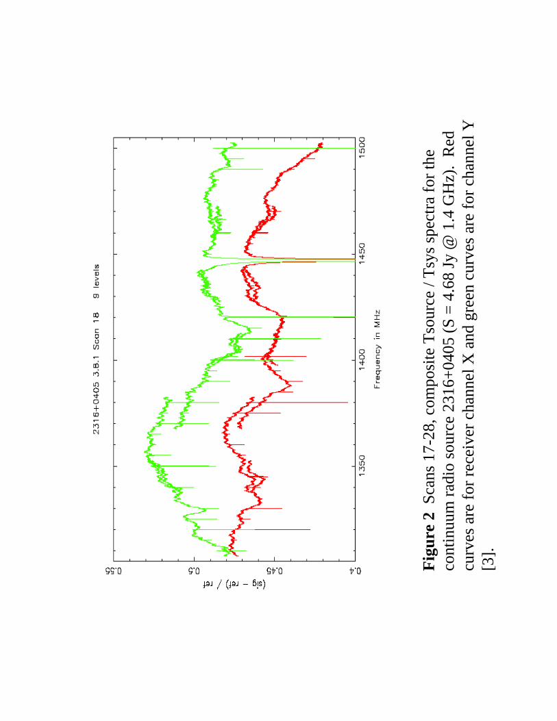
Fig

ure

2Sc

ans

17-2

8, c

ompo

site

Tso

urce

/Tsy

ssp

ectr

a fo

r th

e co

ntin

uum

rad

io s

ourc

e 23

16+0

405

(S =

4.6

8Jy

@ 1

.4 G

Hz)

. R

ed

curv

es a

re f

or r

ecei

ver

chan

nel X

and

gre

en c

urve

s ar

e fo

r ch

anne

l Y

[3].

Atte

n #1 A

ttn

#2

Fig

ure

3A

DS

sim

ulat

ion

show

ing

nois

e te

mpe

ratu

re o

f th

e tw

o at

tenu

ator

s fo

r va

ryin

g in

put

impe

danc

e. U

pper

pan

el is

for

Atte

nuat

or #

1 an

d th

e lo

wer

pan

elis

for

Atte

nuat

or #

2.

Fig

ure

4R

efle

ctom

etry

mea

sure

men

ts o

f G

BT

L-b

and

feed

, dew

ar tr

ansi

tion,

and

OM

T m

ade

by

S. S

hrik

anth

[8]

.

Fig

ure

5B

lock

dia

gram

of

tran

smis

sion

line

cas

cade

with

cap

acita

nce

load

ing

betw

een

sect

ions

.

Fig

ure

6A

DS

sim

ulat

ion

resu

lts s

how

ing

|S22

| (sh

own

here

as

S44)

and

the

com

plex

inpu

t im

peda

nce

for

the

load

ed tr

ansm

issi

on li

ne c

asca

de s

how

n in

Fig

.5.

Fig

ure

7B

lock

dia

gram

of

atte

nuat

or w

ith th

e lo

aded

tran

smis

sion

line

at i

ts in

put.

Fig

ure

8A

DS

sim

ulat

ion

of th

e ci

rcui

t sho

wn

in F

ig. 7

. T

he n

oise

tem

pera

ture

of

the

circ

uit v

ersu

s fr

eque

ncy

for

Atte

nuat

or #

1 is

dis

play

ed o

n th

e le

ft a

nd th

at o

f A

ttenu

ator

#2

is s

how

n on

the

righ

t.

Fig

ure

9Sc

hem

atic

dia

gram

of

the

HFE

T m

odel

use

d in

the

AD

S si

mul

atio

ns [

9].

Fig

ure

10B

lock

dia

gram

of

the

thre

e-st

age,

sin

gle-

ende

d lo

w n

oise

am

plif

ier

used

in th

e A

DS

sim

ulat

ions

.

Fig

ure

11C

alcu

late

d S-

para

met

ers

for

the

thre

e-st

age

low

noi

se a

mpl

ifie

r m

odel

.

Fig

ure

12C

alcu

late

d no

ise

para

met

ers

and

nois

e te

mpe

ratu

re o

f th

e th

ree-

stag

e lo

w n

oise

am

plif

ier

used

in th

e A

DS

sim

ulat

ions

.

Fig

ure

13C

alcu

late

d no

ise

tem

pera

ture

of

the

thre

e-st

age

low

noi

se a

mpl

ifie

r as

a f

unct

ion

of

inpu

t res

ista

nce

(lef

t) a

nd in

put r

eact

ance

(ri

ght)

at 1

.4 a

nd 1

.7 G

Hz.

1.4

GH

z

1.7

GH

z

2-po

rt n

oise

so

urce

Fig

ure

14L

ow n

oise

am

plif

ier

mod

el w

ith a

noi

se s

ourc

e at

the

inpu

t to

sim

ulat

e an

ant

enna

te

mpe

ratu

re th

at is

con

stan

t with

fre

quen

cy.

Fig

ure

15O

n/O

ff s

eque

nce

invo

lvin

g on

ly th

e lo

w n

oise

am

plif

ier.

Fig

ure

16O

n/of

f se

quen

ce f

or

low

noi

se a

mpl

ifie

r an

d lo

aded

tr

ansm

issi

on li

ne.

Fig

ure

17O

n/of

f se

quen

ce f

or lo

w n

oise

am

plif

ier,

at

tenu

ator

, and

load

ed tr

ansm

issi

on li

ne.

Atte

nuat

or is

0.

1 dB

at 3

00 K

with

Zop

t = 5

0 +j

0 oh

ms.

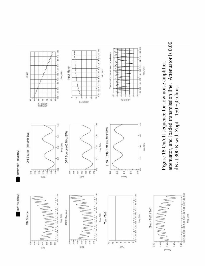
Figu

re 1

8 O

n/of

f se

quen

ce f

or lo

w n

oise

am

plif

ier,

at

tenu

ator

, and

load

ed tr

ansm

issi

on li

ne.

Atte

nuat

or is

0.0

6 dB

at 3

00 K

with

Zop

t= 1

50 +

j0 o

hms.

Fig

ure

19O

n/of

f se

quen

ce f

or lo

w n

oise

am

plif

ier,

atte

nuat

or,

and

load

ed tr

ansm

issi

on li

ne.

Atte

nuat

or is

0.0

6 dB

at 3

00 K

w

ithZ

opt=

150

+j0

ohm

s. L

en2

= 13

5 cm

.

Addendum

Electronics Division Internal Report

No. 312

October 20, 2004

Abstract

NRAO Electronics Division Internal Report 312, published Septem-ber 2, 2003, described investigations into the character and causes of theGreen Bank Telescope spectral baselines. Since publication, several stepshave been taken to further understand and mitigate some of the causesof unsatisfactory baselines. This Addendum to EDIR 312 will reviewthe steps taken and additional knowledge obtained to date, and describefuture plans.

1

1 Review

Spectroscopy in radio astronomy is generally done by measuring the systemoutput spectra under two conditions: one (Sr) with the beam on a referenceposition, and a second (Ss) on the source of interest. On the GBT, the switchingis accomplished by position switching (moving the antenna position), and/or bybeam switching (available at frequencies above 12GHz). To understand theanalysis of position switched data, it is useful to model the receiver chain with apower gain transfer function G(f) and noise temperature Trx(f). As indicated,both of these quantities are functions of frequency and summarize the cascade ofmany active and passive components. Our system consists of the antenna, thereceiver chain, and a spectrometer used to measure the output power spectrum.The equation for the system output power spectrum may be written as:

So(f) = (Tsor(f) + Tant(f) + Trx(f))kBG(f) (1)

where Tsor represents the effective temperature of the antenna main beam,Tant the amalgamation of noise due to atmosphere, background, spillover, etc.,Trx is the noise temperature of the receiver and feed, and kB is the productof Boltzmann’s constant and the effective bandwidth of each spectrometer fre-quency channel. (Note that each noise component is or may be a function offrequency, but from this point on we will omit the (f) except when it seemsimportant to emphasize the frequency variation.) We can now write equationsfor output spectra Ss and Sr. The receiver gain and noise temperature arein general functions of time, if not signal level, so we will also distinguish thegain and noise values during the respective spectral measurements with s andr subscripts.

Sr = (Tref + Tant,r + Trx,r)kBGr (2)

Ss = (Tsig + Tant,s + Trx,s)kBGs (3)

Because the system gain function has relatively large variations with fre-quency, we calculate the ratio of the two scans which under certain conditionswill cancel the gain function:

Ss

Sr− 1 =

Ss − Sr

Sr=

(Tsig + Tant,s + Trx,s)Gs − (Tref + Tant,r + Trx,r)Gr

(Tref + Tant,r + Trx,r)Gr(4)

regrouping we obtain,

Ss − Sr

Sr=

(TsigGs − TrefGr) + (Tant,sGs − Tant,rGr) + (Trx,sGs − Trx,rGr)(Tref + Tant,r + Trx,r)Gr

(5)The quantity of interest is Tsig(f) − Tref (f), and to pluck this value from

equation 5, it is first necessary that the system gain and noise temperature are

2

completely stable over the measurement period. That is Gs = Gr, Tant,s =Tant,r, and Trx,s = Trx,r. Then equation 5 becomes:

Ss − Sr

Sr=

Tsig − Tref

Tref + Tant,r + Trx,r(6)

This equation shows that, even with perfect system stability during themeasurement, the quantity (Ss − Sr)/Sr will only be flat with frequency ifTref +Tant,r +Trx,r is flat, or Tsig−Tref is very small over most of the frequencyrange. The denominator of equation 6 is just Tsys(f) during the reference scan,so multiplying by that value will retrieve the desired quantity Tsig−Tref . Tsys,r

is usually determined by using a small injected noise cal, but for flat baselinesTsys,r, and hence Tcal, must be determined to a high accuracy at every frequencyin the passband. The importance of this increases as the average differencebetween Tsig and Tref gets larger (spectroscopy on continuum sources). Inthe past, spectral data analysis has generally assumed a constant Tcal and/orTsys across the spectrum, or at most a fit to a few points, but with the broadbandwidths available from the GBT spectrometer, in many cases that turns outto be an unsatisfactory approach.

It is clear from this discussion that gain or noise temperature changes duringa measurement will prevent the cancellation of quantities in equation 5. And,ripple in Tsys must be minimized or measured accurately in order to cancel thedenominator of equation 6.

The past year’s work on GBT baselines has focused on three broad areas:

Gain Stability The degree of stability required is challenging. Most of theidentified problems were related to coaxial interconnections, and were ad-dressed by improved testing and assembly procedures.

Standing Waves As discussed in the body of EDIR 312, standing waves im-pact the system by producing frequency structure in both gain and noisetemperature. The standing wave stability is affected by changes in mis-match magnitude or phase, and by changes in the electrical length oftransmission paths. The effects can be attacked by reducing the magni-tude of mismatches, stabilizing the electrical length of transmission lines,or shortening transmission lines (which increases the period of the rippleand may make it easier to tolerate).

Receiver Noise Ripple Extensive testing has shown that frequency structurein receiver noise temperature is a major source of difficulties in observingstrong continuum sources. Little progress beyond what was described inthe body of EDIR 312 has been made in reducing the structure, but someprogress has been made in the understanding and in calibration methods.

Discussion of specific areas of work follow.

3

2 Coaxial Cables

PTFE (Teflon), the most common dielectric found in microwave cables, has anunfortunate transition in its physical properties near room temperature. Thatleads to high sensitivity of electrical length to temperature (about 100ppm/◦C).As described in EDIR 312, section 4.4, a couple of varieties of Andrews Heliaxtype cables using polyethylene dielectric have significantly better temperaturecoefficients, and have been installed in several critical locations. Occasionalproblems with the FSJ1-50A Heliax developed due to shearing of the copperjacket at the SMA connector clamp-on backshell. These failures caused gaininstabilities that were intermittant and position dependent. An assembly pro-cedure was developed that supplemented the clamp with epoxy potting, andhas largely eliminated cable failures due to this cause. Connector problemswith other Heliax cable types have occurred, and one must be careful in theiruse, despite the attractive performance of the cable itself.

Longer PTFE cables in the Equipment Room between the Converter Racksand the Spectrometer were placed in conduits to buffer air temperature fluc-tuations. These cables carry lower frequencies and the cost of retrofitting toHeliax does not yet seem necessary. Ripple components consistent with the ca-ble lengths have not been observed in baselines since the buffering was installed.

3 Feed Radomes

The Gregorian feeds have woven PTFE sheets over the feed apertures, and wateron this surface leads to reflections that are unstable as the water moves around.The radome blower system was upgraded to increase the air flow, significantlyimproving the removal of water beads.

The original radome designs used flat metal rings to clamp the PTFE sheetsto the feed horns. That led to a recess in which water tended to puddle. Allthe feeds at X-band and above have now been retrofitted to use a wrap-arounddesign for radome attachment, eliminating the recess.

4 Converter Rack

EDIR 312 section 4.5 described a persistant baseline ripple component withperiod near 60MHz, whose origin had been isolated to the Converter Racks andwas closely related to the Equipment Room temperature. The magnitude of thisripple ranged up to about 0.5% of the total power. The generating mechanismwas not well understood however, and effort was spent both to improve thetemperature stability, and to understand how the ripple was generated.

Figure 1 shows a simplified view of the interface between the IF OpticalReceiver and the 1-8 GHz Converter modules. The IF signal is amplified andsplit four ways in the Optical Receiver,and then goes to four Converter modules(only two of the four Converter modules are shown in the figure). The base-line ripple generating mechanism is understood by tracing a signal through the

4

diagram: A signal leaves the amplifier and is split four ways in the power di-vider, which has electrical delay Θd. The one-fourth signal that exits the lowerport travels through a fairly long coaxial cable with delay Θ2 and enters theConverter module input switch and mixer. However, a portion of the signal isreflected by reflection coefficient ρ2, back thru the cable delay Θ2 and the powerdivider and into the amplifier output port. At the amplifier output, a portionis reflected, ρa, and reenters the splitter input. So, the total signal that entersthe top converter module mixer is the vector sum of one-fourth of the amplifieroutput signal, and a smaller component which has travelled through Θd andΘ2 twice. (And two other components off the other two converter modules notshown.) These reflected signals cause standing waves and hence gain rippleswith frequency. Note that if the phase of the reflected signals change due to,say, change in the electrical phase of the cable delay Θ2, or reflection coefficientsρ2 or ρa, the gain ripple will change resulting in baseline ripples. Early on, themechanism of change in the cable delay was recognized and phase stable cableswere installed. However, the ripples were still apparent and the search beganfor other causitive mechanisms. In the end, the problems were found to bedominated by a few highly sensitive, defective components - RF switches, pads,etc. Because a defective component affects the response of four channels andthe effects tend to be too small to detect with common test equipment, isolatingthe problems proved to be difficult.

Figure 2 shows a series of two-minute off/on baselines taken through thesystem illustrating the improvements that have been achieved. Although signif-icant improvements have been made, some ripple is still apparent. This rippledoes tend to average out over many off/on pairs. The final solution howeverprobably lies in repackaging of this area of the system to greatly shorten thepathlengths involved and to provide improved thermal buffering.

5

Figure 1: A simplified block diagram of the Optical Receiver - Converter Moduleinterface.

5 Receiver Noise

5.1 Introduction

Section 3 of EDIR 312 discussed spectral baselines on continuum sources. Itwas recognized that receiver noise which varies with frequency is a potentialsource of baseline problems because usual data analysis techniques assumed aconstant Tsys(f). The search for causes of ripple in receiver noise focused onthe receiver input area - between the feed aperture and the first LNA - and infact a few specific problems were identified and corrected as discussed in theoriginal report. However, it became clear that this was not the whole story- the shape of the baselines were too irregular and the period of ripples didnot match physical lengths that could set up standing waves. One difficultityin understanding the problem was because our normal laboratory equipmentand methods of measuring noise temperature provided frequency resolution toocoarse to be of much use. However, the GBT spectrometer obviously providesa means to obtain high-resolution spectra, and as long as the total power doesnot change by more than 3dB or so, we felt it could be used to perform ahot-cold noise temperature measurement. We put together an experiment usingcomponents taken from the GBT 40-52 GHz Q-band receiver, with care taken toeliminate the possibility of input mismatch or resonances affecting the results.

A test arrangement consisting of a cooled LNA and mixer, IF filter, and IFamplifier were taken from the Q-band receiver and placed in one of our testdewars. The LNA input port was connected to a cooled rectangular waveguideload. The load was thermally separated from the LNA with a 1 cm stainlesssteel waveguide shim. A small heater and temperature sensor allowed the load

6

Figure 2: IF system baseline ripples due to Equipment Room temperature be-fore (top panel) and after (bottom panel) improvements to the Converter Rackequipment.

7

temperature to be adjusted by 10-15K. Measurements on the stainless shim andthe load show that the combination has a return loss of 32 dB or better.

The test dewar was located in the Equipment Room and the IF output(centered at 6 GHz) was connected into the GBT IF system via heliax cable.The system and the spectrometer were then configured for 800 MHz bandwidthmeasurements of the spectrum.

5.2 The Y-factor Method

The most common engineering method of determining a receiver’s noise temper-ature is to measure its output power with two known input source temperatures.The ratio of the two powers is termed the Y-factor. Since a spectrometer mea-sures the spectral power versus frequency, we can use two measurements takenwith two source temperatures to obtain Y (f):

Y (f) =Shot

Scold=

(Thot + Trx,hot(f))kBGs

(Tcold + Trx,cold(f))kBGr(7)

Again assuming receiver stability, and solving for Trx, we obtain a familiarequation:

Trx(f) =Thot − Y (f)Tcold

Y (f)− 1(8)

5.3 Q-band Laboratory Data

Spectra were measured with two load temperatures differing by about 15K,and the data used to calculate Trx(f) using equations 7 and 8. Figure 3 plotstypical Trx using this method. To check linearity and stability of the data,several subsequent scans taken at a variety of load temperatures were processedthrough the baseline equations using this measured Trx. Figure 4 shows theeffect on spectral baselines when the measured Trx is used in equation 6.

The fact the input load return loss was quite low makes a strong case thatthe source match seen by the LNA can not explain the noise structure seen inthese measurements. Subsequent work indicates that in this receiver mixer noiseis a significant contributor to the total receiver noise structure, and can perhapsbe mitigated by increasing the gain before the mixer and by terminating theimage and other sideband frequencies with low VSWR. Work along these linesis on-going, and may lead to similar investigations in other receivers.

5.4 X-band Astronomical Data

Because of the laboratory results, it seemed possible that the Trx variations havebeen a major source of baseline structure when observing continuum sources.And, it might be possible to use astronomical observations to measure Trx forsubsequent use in baseline data analysis.

8

Figure 3: Trx at 42 GHz (upper panel)and 43 GHz (lower panel), obtainedfrom a test dewar containing a Q-band LNA and cooled mixer, calculated withequations 7 and 8. A heated waveguide termination was used to vary the LNAinput load temperature.

9

Figure 4: The upper plot shows the spectral baselines on the Q-band test dewarsetup for several signal scans taken at various load temperatures. The greentraces were calculated using a mean Trx of 15.5K, and the other (flatter) tracesused measured Trx(f). The lower panel zooms into the region around 7 K.

10

To see how the Y-factor measurement of Trx(f) behaves with a front-endoperating on the GBT, astronomical data previously taken with the X-bandreceiver was analyzed. The first data set consisted of a sequence of on-off ob-servations of NGC 7027. One observation was used to calculate Trx, and thatvalue used to analyze subsequent observations. Only one source was observed,but the data can provide an indication of the stability of the analysis. Examplesfrom this dataset are shown in Figures 5 and 6.

The second X-band data set analyzed was a sequence of on-off observationsof three sources. By coincidence, one of the sources was NGC 7027, and thatsource was used to determine Trx applied to analysis of the other sources. Theresults are shown in Figures 7 and 8.

It is clear from these figures that the technique used here has promise inremoving major portions of the baseline structure on continuum sources. How-ever, other uncertainties are introduced by the need to understand well thespectral signature of calibrator sources. Work continues to develop the best andmost practical observing and analysis procedures.

11

Figure 5: X-band spectral baselines calculated for TBASERDN030926 scan pair24 and 25, ACS Bank A. The red trace was calculated using Trx measured usingscan pair 22 and 23 data as a Hot/Cold measurement. The green trace wascalculated using a constant Tsys, and the blue trace used a Tsys derived fromCal On - Cal Off data in scan 25. The vertical scale corresponds to TOn−TOff

in Kelvin. The lower panel shows the red and green traces in more detail. Forthese plots 400MHz on the horizontal axis corresponds to a sky frequency of9000MHz, and sky frequency increases to the right. The data was from theRCP polarization.

12

Figure 6: X-band spectral baselines calculated for TBASERDN030926 scanpair 24 and 25, ACS Bank D, calculated in three ways. The red trace wascalculated using Trx measured using scan pair 22 and 23 data as a Hot/Coldmeasurement. The green trace was calculated using a constant Tsys, and theblue trace used a Tsys derived from Cal On - Cal Off data in scan 25. Thevertical scale corresponds to TOn − TOff in Kelvin. The lower panel shows thered and green traces in more detail. For these plots 400MHz on the horizontalaxis corresponds to a sky frequency of 9600MHz, and sky frequency increasesto the right. The data was from the RCP polarization.

13

Figure 7: X-band spectral baselines for TPCO1A402 scan pair 16 and 17, on2052−3635, calculated in three ways. The red trace was calculated using Trx

measured using scan pair 14 and 15, NGC 7027 data, as a Hot/Cold measure-ment. The green trace was calculated using a constant Tsys, and the blue traceused a Tsys derived from Cal On - Cal Off data in scan 17. The vertical scalecorresponds to TOn−TOff in Kelvin. The lower panel shows the red and greentraces in more detail. For these plots 400MHz on the horizontal axis correspondsto a sky frequency of 9900MHz, and sky frequency increases to the right. Thedata was from the RCP polarization.

14

Figure 8: X-band spectral baselines for TPCO1A402 scan pair 18 and 19, on2202+422, calculated in three ways. The red trace was calculated using Trx

measured using scan pair 14 and 15, NGC 7027 data, as a Hot/Cold measure-ment. The green trace was calculated using a constant Tsys, and the blue traceused a Tsys derived from Cal On - Cal Off data in scan 19. The vertical scalecorresponds to TOn−TOff in Kelvin. The lower panel shows the red and greentraces in more detail. For these plots 400MHz on the horizontal axis correspondsto a sky frequency of 9900MHz, and sky frequency increases to the right. Thedata was from the RCP polarization.

15

6 Conclusions

The understanding of GBT spectral baseline characteristics has significantlyimproved since the onset of observations. Baseline improvements have beenincremental, but significant. The requirements on the GBT hardware are strin-gent, as in all radio astronomy systems, particularly due to the relatively highintermediate frequencies and broad bandwidths used, and the system complex-ity caused by the need to support multiple backends and multiple simultaneousspectral observations.

The frequency structure in receiver noise which has a serious impact oncontinuum source observations requires more research until the causes are wellunderstood. However, in the meantime there is promise in improvements toobserving and analysis procedures.

The understanding gained in the course of the baseline investigations couldbe applied to the design of an “ideal” spectral line receiver. The approach wouldlikely evolve toward a highly integrated design, using quite short transmissionlines and a minimum of coaxial interconnections, in an isothermal package. Theintegration of digital samplers with the microwave front-end should be investi-gated. It is likely that an improved receiver design would make observations forbroad spectral lines much more feasible with the GBT.

16