Full Terms & Conditions of access and use can be found athttps://www.tandfonline.com/action/journalInformation?journalCode=nsie20

Structure and Infrastructure EngineeringMaintenance, Management, Life-Cycle Design and Performance

ISSN: 1573-2479 (Print) 1744-8980 (Online) Journal homepage: https://www.tandfonline.com/loi/nsie20

Investigation of the effect of the inspectionintervals on the track geometry condition

Iman Soleimanmeigouni, Alireza Ahmadi, Hamid Khajehei & Arne Nissen

To cite this article: Iman Soleimanmeigouni, Alireza Ahmadi, Hamid Khajehei & Arne Nissen(2019): Investigation of the effect of the inspection intervals on the track geometry condition,Structure and Infrastructure Engineering, DOI: 10.1080/15732479.2019.1687528

To link to this article: https://doi.org/10.1080/15732479.2019.1687528

© 2019 The Author(s). Published by InformaUK Limited, trading as Taylor & FrancisGroup

Published online: 20 Nov 2019.

Submit your article to this journal

View related articles

View Crossmark data

Investigation of the effect of the inspection intervals on the trackgeometry condition

Iman Soleimanmeigounia, Alireza Ahmadia, Hamid Khajeheia and Arne Nissenb

aDivision of Operation and Maintenance Engineering, Luleå University of Technology, Luleå, Sweden; bTrafikverket, Luleå, Sweden

ABSTRACTIn order to evaluate the railway track geometry condition and plan maintenance activities, track inspec-tion cars run over the track at specific times to monitor it and record geometry measurements. Applyingan adequate inspection interval is vital to ensure the availability, safety and quality of the railway track,at the lowest possible cost. The aim of this study has been to investigate the effect of different inspec-tion intervals on the track geometry condition. To achieve this, an integrated statistical model was devel-oped to predict the track geometry condition given different inspection intervals. In order to model theevolution of the track geometry condition, a piecewise exponential model was used which considersbreak points at the maintenance times. Ordinal logistic regression was applied to model the probabilityof the occurrence of severe isolated defects. The Monte Carlo technique was used to simulate the trackgeometry behaviour given different inspection intervals. The results of the proposed model support thedecision-making process regarding the selection of the most adequate inspection interval. The applic-ability of the model was tested in a case study on the Main Western Line in Sweden.

ARTICLE HISTORYReceived 17 May 2019Revised 28 July 2019Accepted 3 September 2019

KEYWORDSInspection; track geometry;maintenance; multivariablelinear regression; isolateddefects; ordinallogistic regression

1. Introduction

The railway track geometry is subjected to degradationmainly due to the forces induced by traffic, which causedeviations from the designed vertical and horizontal align-ments. When a geometry defect occurs, the consequencescan be significant, including economic loss, damage to theenvironment and, in severe cases, the possible loss of humanlives. In order to protect against unacceptable consequences,track geometry maintenance actions are planned to retainthe geometry condition in or restore it to an acceptable statewith respect to ride comfort and the safety limits. In orderto have an effective and efficient maintenance plan, thetrack geometry condition must be inspected on a regularbasis. The main aims of geometry inspection are to deter-mine the deviation of geometry parameters from acceptablelimits, and to enable prediction of the time remaining untilthe intervention and safety limits are reached (UIC, 2008).The frequency of inspection is highly important as it affectsthe detectability of geometry defects and the associatedmaintenance requirements. As a result, a proper inspectioninterval is a key factor for determining the performanceof line sections, controlling and reducing the risk ofderailment and the maintenance cost, and keeping thepunctuality of train operations at the highest level.Various factors are involved in the selection of an applic-able and effective inspection interval, including the trafficprofile, the regulatory requirements, the level of risk intrain operations, and the maximum allowable speed of

trains (American Railway Engineering and Maintenance-of-Way Association (AREMA), 2006).

In recent years, a number of researchers have tried todetermine an optimal inspection interval with respect to dif-ferent objective functions. Arasteh Khouy, Larsson-Kråik,Nissen, Juntti, and Schunnesson (2014) optimized the trackgeometry inspection intervals with the objective of minimiz-ing the total maintenance cost. In the proposed model, pre-ventive and corrective tamping is executed based on theQ-value indicator and severe defects of twist, respectively. Asimilar approach can be found in Soleimanmeigouni,Ahmadi, Letot, Nissen, and Kumar (2016), who attemptedto determine a cost-effective track geometry inspectioninterval. They considered the standard deviation of the lon-gitudinal level as the dominant factor for evaluation of thetrack condition. They used the Wiener process to model thetrack geometry degradation. Lyngby, Hokstad, and Vatn(2008) conducted research to optimize the intervals of trackgeometry inspection with the same objective. They appliedthe Markov methodology to model the track geometry deg-radation. In their study, twist was considered as a trackquality indicator. In the model proposed by Lyngby et al.(2008), the corrective and preventive activities are assumedto be perfect. Meier-Hirmer, Sourget, and Roussignol (2005)conducted a case study and determined a trade-off betweenthe inspection interval and the maintenance threshold thatleads to the minimum track maintenance cost. The trackgeometry degradation and tamping effectiveness were

CONTACT Iman Soleimanmeigouni iman.meigouni@ltu.se Division of Operation and Maintenance Engineering, Luleå University of Technology, Luleå 97187, Sweden� 2019 The Author(s). Published by Informa UK Limited, trading as Taylor & Francis GroupThis is an Open Access article distributed under the terms of the Creative Commons Attribution-NonCommercial-NoDerivatives License (http://creativecommons.org/licenses/by-nc-nd/4.0/),which permits non-commercial re-use, distribution, and reproduction in any medium, provided the original work is properly cited, and is not altered, transformed, or built upon in any way.

STRUCTURE AND INFRASTRUCTURE ENGINEERINGhttps://doi.org/10.1080/15732479.2019.1687528

modelled using the gamma process and linear regression,respectively. In this study, the maintenance was carried outon track sections with a fixed delay after detection.

More recently, Osman, Kaewunruen, Jack, and Sussman(2016) conducted research on the possibility of consideringa ‘plan B’ or contingency plan in track inspection schedules.This ‘plan B’ would reschedule the inspection plan in theevent of an incident happening which would affect the cur-rent inspection schedule. A different approach can be seenin a study presented by Andrews, Prescott, and De Rozi�eres(2014), who did not include an objective function in theirwork. They studied the effect of different inspection strat-egies on the quality of the track geometry. The standarddeviation of the longitudinal level was used as a measure-ment of the track geometry quality. They reported that, des-pite their expectations, different inspection intervals did nothave a significant effect on the total number of maintenanceactions. However, they ascertained that the longer theinspection intervals were, the larger was the proportion ofmaintenance which had to be carried out on track withpoorer quality. Moreover, Andrews et al. (2014) pointed outthat a decrease in the frequency of inspections wouldincrease the percentage of time during which the trackwould need emergency maintenance.

Obviously, an effective inspection regime can be developedaccording to an assessment of the effect of different inspectionintervals on the track performance. The performance of thetrack can be measured by determining the percentage of timespent by the track sections in different geometry states. Thesestates can be defined based on the maintenance limits. The aimof the present study has been to develop an integrated approachto investigate the effect of different inspection intervals on theperformance of the track. A fundamental requirement forachieving this aim is long-term prediction of the track geometrycondition by modelling and integrating: (1) the track geometrydegradation; (2) the tamping recovery; (3) the occurrence ofsevere isolated defects. In this study, to characterize the trackgeometry degradation and restoration, a piecewise exponentialmodel was applied which considers break points at the main-tenance times. A multivariable linear regression model wasused to link different covariates to the tamping recovery. Inaddition, ordinal logistic regression was applied to predict theprobability of the occurrence of isolated defects. Due to theexistence of variation in the model parameters, the MonteCarlo technique was used to estimate the percentage of timespent in different track geometry states. In order to verify the

applicability of the model, a case study was performed with datacollected from the MainWestern Line in Sweden.

The rest of this paper is organized as follows. Section 2contains background information on the track geometryparameters and maintenance limits. Section 3 describes theprocess of track geometry measurement. Section 4 dealswith the analytical models and the proposed approach. Thecase study is presented in Section 5 and, finally, Section 6provides the conclusions.

2. Track geometry parameters andmaintenance limits

Track geometry parameters are widely used to represent thetrack condition and to plan maintenance activities. Trackgeometry parameters can be divided into five classes, i.e. thelongitudinal level, alignment, gauge, can’t, and twist. Thelongitudinal level is the geometry of the track centrelineprojected onto the longitudinal vertical plane. The align-ment is the geometry of the track centreline projected ontothe longitudinal horizontal plane. The gauge is the distancebetween the gauge faces of two adjacent rails at a givenlocation below the running surface. The cant (cross-level) isthe difference in height between the adjacent running tablescomputed from the angle between the running surface anda horizontal reference plane. The twist is the algebraic dif-ference between two cross-levels taken at a defined distanceapart, usually expressed as a gradient between the twopoints of measurement (SS-EN 13848-1: 2004þA1, 2008).

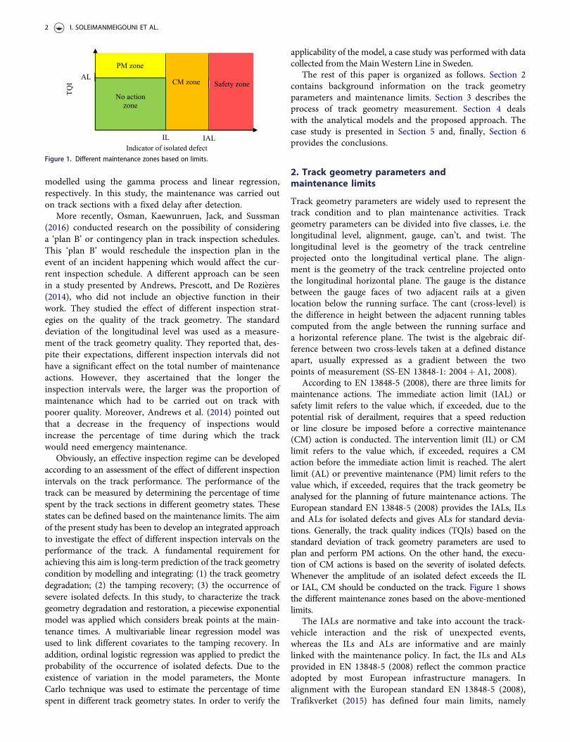
According to EN 13848-5 (2008), there are three limits formaintenance actions. The immediate action limit (IAL) orsafety limit refers to the value which, if exceeded, due to thepotential risk of derailment, requires that a speed reductionor line closure be imposed before a corrective maintenance(CM) action is conducted. The intervention limit (IL) or CMlimit refers to the value which, if exceeded, requires a CMaction before the immediate action limit is reached. The alertlimit (AL) or preventive maintenance (PM) limit refers to thevalue which, if exceeded, requires that the track geometry beanalysed for the planning of future maintenance actions. TheEuropean standard EN 13848-5 (2008) provides the IALs, ILsand ALs for isolated defects and gives ALs for standard devia-tions. Generally, the track quality indices (TQIs) based on thestandard deviation of track geometry parameters are used toplan and perform PM actions. On the other hand, the execu-tion of CM actions is based on the severity of isolated defects.Whenever the amplitude of an isolated defect exceeds the ILor IAL, CM should be conducted on the track. Figure 1 showsthe different maintenance zones based on the above-mentionedlimits.

The IALs are normative and take into account the track-vehicle interaction and the risk of unexpected events,whereas the ILs and ALs are informative and are mainlylinked with the maintenance policy. In fact, the ILs and ALsprovided in EN 13848-5 (2008) reflect the common practiceadopted by most European infrastructure managers. Inalignment with the European standard EN 13848-5 (2008),Trafikverket (2015) has defined four main limits, namely

Figure 1. Different maintenance zones based on limits.

2 I. SOLEIMANMEIGOUNI ET AL.

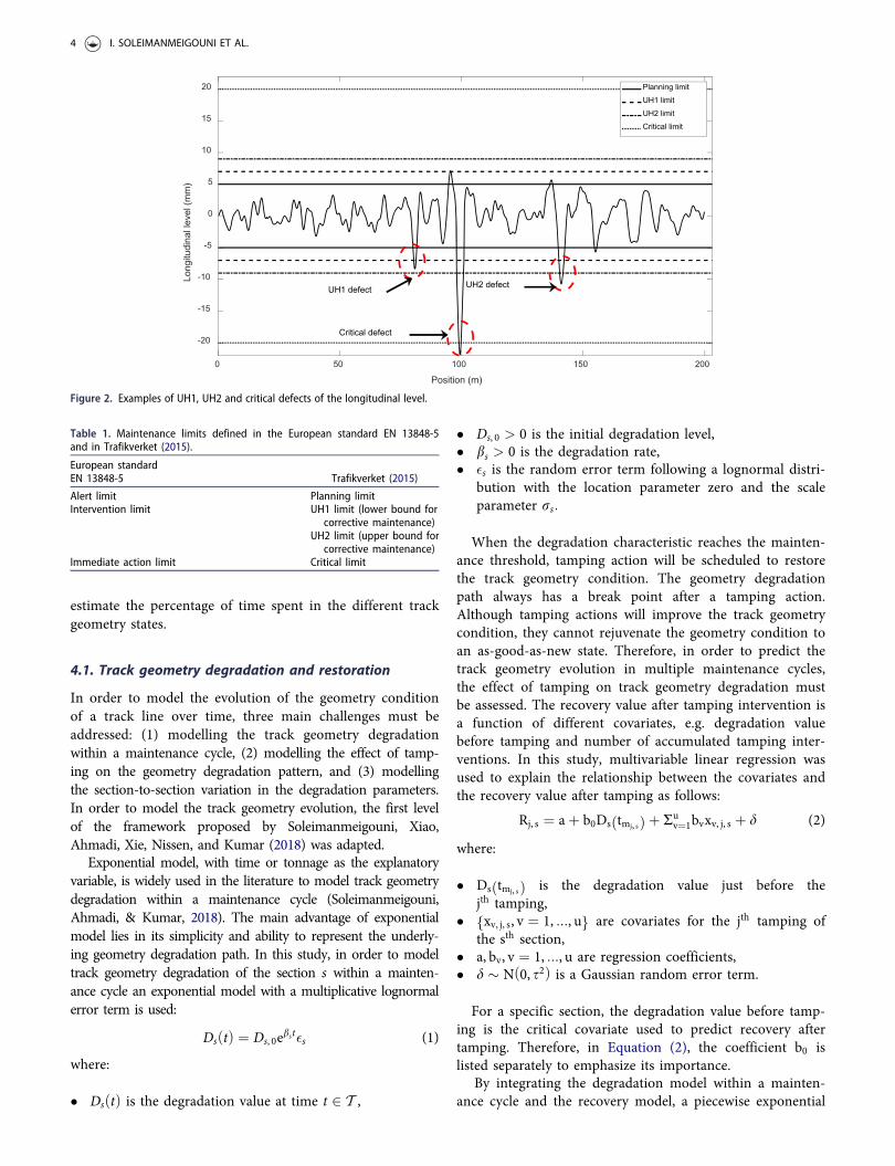
the planning limit, the UH1 and the UH2 limit, and thecritical limit, as can be seen in Figure 2. In Trafikverket(2015) the intervention limit is expressed as a range ratherthan as a discrete value. Track irregularities that exceed theUH1 limit must be assessed for conducting maintenancebefore the UH2 limit is exceeded. For track irregularitiesexceeding the UH2 limit, a maintenance action must beplanned without unnecessary delay. Therefore, track irregular-ities must be corrected before the UH2 limit is reached. Table1 presents the relation between the limits defined in EN13848-5 (2008) and those defined in Trafikverket (2015).

Based on the above-mentioned limits, geometry defectscan be classified according to their severity into threegroups, i.e. UH1, UH2 and critical defects. UH1, UH2 andcritical defects occur when track irregularities exceed theUH1, UH2 and critical limits, respectively. Examples ofthese three categories of defects are shown in Figure 2.

3. Track geometry inspection

The main objectives of measuring the track geometry are to:(1) locate the occurrence of severe isolated defects and pri-oritize the CM actions required to rectify them, (2) to planthe PM actions, (3) to evaluate the effectiveness and qualityof conducted maintenance activities, and (4) to establish theeffectiveness and adequacy of financial expenditure(Zaayman, 2017). The track geometry measurement car isan automated track inspection vehicle whose purpose is tomeasure and record the track geometry in real time and todisplay the measurements obtained. The vehicle measuresvarious geometry parameters, e.g. the longitudinal level,alignment, can’t, gauge, twist, curve radius, and gradient ata specific sampling interval.

The measured data are available in three forms, i.e.on-board network viewing of measurements, on-board real-time reports, and off-board post-processed reports. Theon-board real-time reports can be used to address severeisolated defects and comprise strip charts and exceptionsreports. The strip chart is a graphical representation of theoverall track geometry condition in one picture and displaysall the track geometry measurements and the correspondingmaintenance limits. The strip chart shows when a particularmeasurement approaches or exceeds the maintenance limits.When the track geometry measurements exceed the main-tenance limits, a geometry defect will appear in the excep-tions report.

The purpose of the exceptions report is to provide a listof all the geometry defects found by the track geometrymeasurement vehicle during the inspection of the track. Thebasic information provided in the exceptions report is thedefect name, the position of the defect, and the defectlength, defect magnitude, maintenance limit, and maximumallowable speed. Using the strip charts and the exceptionsreports aids the process of conducting CM activities toavoid the occurrence of severe isolated defects which maycause catastrophic consequences. In addition to on-boardreports, the geometry measurements are post-processed intodifferent standard reports. These reports can be used for

further analysis of the track geometry condition to supporttrack maintenance decision making to achieve a robust andcost-effective maintenance plan. Analysing the track geom-etry measurements and aggregating them into a track qual-ity index (TQI) can aid the planning of track geometrymaintenance activities. By performing a statistical analysison the evolution of the TQIs, the trends in the track geom-etry degradation can be identified. In addition, the measureddata can be used to identify potentially hazardous trackgeometry conditions.

4. Proposed methodology

Figure 3 provides a schematic description of the proposedanalytical model. As can be seen, the track geometry isinspected at discrete time intervals (s) to determine its con-dition. At each inspection, the standard deviation of thegeometry parameters and the extreme values of isolateddefects are recorded. According to the results of the trackgeometry inspection, different intervention decisions can bemade to retain the geometry condition in or to restore it toan acceptable state. With reference to the maintenance lim-its explained in Section 2, after each inspection, one of thefollowing three actions may be taken.

� Preventive maintenance: If the standard deviation of thegeometry parameters exceeds the planning limit, then thetrack section is assessed for PM to be performed inthe first available maintenance window. By schedulingthe PM for the time periods planned for maintenanceinterventions, the maintenance will be performed in away which will neither interrupt the normal traffic norcause traffic delays.

� Normal corrective maintenance (CMn): When a UH2defect occurs, a CM action is conducted on the tracksection. Railway companies need short-term plans foradjusting the traffic by cancelling, postponing or rerout-ing trains to provide time to conduct CM actions. Suchshort-term plans provide a period of time during whichthe track can be operated until maintenance takes place.

� Emergency corrective maintenance (CMe): When a criticaldefect occurs, an immediate CM action with a speed reduc-tion or line closure is carried out on the track section.

Figure 3 depicts the three above-mentioned situations.The aim of the proposed analytical model is to predict thepercentage of time which the track spends in the differenttrack geometry states using various inspection intervals.With reference to the maintenance limits explained inSection 2, Table 2 presents the different geometry states.Owing to the complexity of the degradation process and themaintenance process, predicting the effect of employing dif-ferent inspection intervals on the track geometry conditionis a difficult task (Andrews et al., 2014; Quiroga &Schnieder, 2012). Therefore, the Monte Carlo simulationtechnique is used to handle the variation of the variousparameters within the proposed integrated model and to

STRUCTURE AND INFRASTRUCTURE ENGINEERING 3

estimate the percentage of time spent in the different trackgeometry states.

4.1. Track geometry degradation and restoration

In order to model the evolution of the geometry conditionof a track line over time, three main challenges must beaddressed: (1) modelling the track geometry degradationwithin a maintenance cycle, (2) modelling the effect of tamp-ing on the geometry degradation pattern, and (3) modellingthe section-to-section variation in the degradation parameters.In order to model the track geometry evolution, the first levelof the framework proposed by Soleimanmeigouni, Xiao,Ahmadi, Xie, Nissen, and Kumar (2018) was adapted.

Exponential model, with time or tonnage as the explanatoryvariable, is widely used in the literature to model track geometrydegradation within a maintenance cycle (Soleimanmeigouni,Ahmadi, & Kumar, 2018). The main advantage of exponentialmodel lies in its simplicity and ability to represent the underly-ing geometry degradation path. In this study, in order to modeltrack geometry degradation of the section s within a mainten-ance cycle an exponential model with a multiplicative lognormalerror term is used:

Ds tð Þ ¼ Ds, 0ebst�s (1)

where:

� Ds tð Þ is the degradation value at time t 2 T ,

� Ds, 0 > 0 is the initial degradation level,� bs > 0 is the degradation rate,� �s is the random error term following a lognormal distri-

bution with the location parameter zero and the scaleparameter rs:

When the degradation characteristic reaches the mainten-ance threshold, tamping action will be scheduled to restorethe track geometry condition. The geometry degradationpath always has a break point after a tamping action.Although tamping actions will improve the track geometrycondition, they cannot rejuvenate the geometry condition toan as-good-as-new state. Therefore, in order to predict thetrack geometry evolution in multiple maintenance cycles,the effect of tamping on track geometry degradation mustbe assessed. The recovery value after tamping intervention isa function of different covariates, e.g. degradation valuebefore tamping and number of accumulated tamping inter-ventions. In this study, multivariable linear regression wasused to explain the relationship between the covariates andthe recovery value after tamping as follows:

Rj, s ¼ aþ b0Ds tmj, sð Þ þ Ruv¼1bvxv, j, s þ d (2)

where:

� Ds tmj, sð Þ is the degradation value just before thejth tamping,

� xv, j, s, v ¼ 1, :::, uf g are covariates for the jth tamping ofthe sth section,

� a, bv, v ¼ 1, :::, u are regression coefficients,� d � N 0, s2ð Þ is a Gaussian random error term.

For a specific section, the degradation value before tamp-ing is the critical covariate used to predict recovery aftertamping. Therefore, in Equation (2), the coefficient b0 islisted separately to emphasize its importance.

By integrating the degradation model within a mainten-ance cycle and the recovery model, a piecewise exponential

Figure 2. Examples of UH1, UH2 and critical defects of the longitudinal level.

Table 1. Maintenance limits defined in the European standard EN 13848-5and in Trafikverket (2015).

European standardEN 13848-5 Trafikverket (2015)

Alert limit Planning limitIntervention limit UH1 limit (lower bound for

corrective maintenance)UH2 limit (upper bound for

corrective maintenance)Immediate action limit Critical limit

4 I. SOLEIMANMEIGOUNI ET AL.

model was applied to characterize the degradation in mul-tiple maintenance cycles as follows:

Ds tð Þ ¼Ds, 0

Pksj¼1Rj, sI t>tmj, sð Þ

e bstð Þ�s (3)

where:

� tmj, s is the time of the jth tamping for the sth track section,� ks is the number of tamping interventions on the sth

track section,� I �ð Þ is the indicator function.

Due to the variability of the track structure, traffic condi-tions, environmental conditions, and maintenance history, thereis section-to-section variation in the degradation parameters. Inthe degradation model applied in this study, the initial degrad-ation value and degradation rates are considered as log-nor-mally distributed random variables. This is in accordance withthe findings of a study by Soleimanmeigouni et al. (2018).

4.2. Occurrence of severe isolated defects

In order to consider CM actions in the developed model, it isneeded to model the occurrence of UH2 defects and criticaldefects. The probability of occurrence of severe isolated defectsis dependent on the typical track quality indices used to planmaintenance activities (Andrade & Teixeira, 2013). Therefore,in order to estimate the probability of the occurrence of UH2defects and critical defects, ordinal logistic regression with TQIas the explanatory variable was applied in this study.

4.2.1. Ordinal logistic regressionLogistic regression is a well-known statistical method indata analysis for describing the relationship between a dis-crete response variable, taking on two or more possible val-ues, and a set of explanatory variables. (Hosmer, Lemeshow,& Sturdivant, 2013). When a response variable has only twopossible values, the binary logistic regression model iswidely used as a standard method of analysis. In the field of

track geometry degradation modelling and maintenanceplanning, binary logistic regression was applied to predict theoccurrence of isolated defects. C�ardenas-Gallo, Sarmiento,Morales, Bolivar, and Akhavan-Tabatabaei (2017) applied bin-ary logistic regression to identify the relationship between a setof explanatory variables including; defect amplitude, traffic,and class of track; and the future state of the isolated defects.Andrade and Teixeira (2013), used binary logistic regression topredict the probability of the occurrence of isolated defects.They considered the standard deviation of the longitudinallevel and alignment, and the existence of a switch or bridge ina section as explanatory variables.

It must be noted that if the binary logistic regression beused, only two outcomes can be predicted: no isolated defectin the track section or at least one isolated defect in thetrack section. In the case of the present paper, the isolateddefects are divided into multiple discrete categories basedon their severity. In order to handle this situation an exten-sion of typical logistic regression must be applied. When theresponse variable is rank-ordered or ordinal with more thantwo levels, ordinal logistic regression can be used to estimatethe probability that the response variable is classified intoone of the outcomes. Therefore, in order to estimate theprobability of the occurrence of UH2 defects and criticaldefects, the ordinal logistic regression model is used.

In ordinal logistic regression, by considering Y as anordinal response variable which can take on kþ 1 valuescoded 0, 1, 2, :, k, the cumulative logit transformation of Yis modelled as the linear function of the explanatory varia-bles as follows:

logitðY � kÞ ¼ gk xð Þ ¼ logPðY � kÞ

1� PðY � kÞ

� �

¼ hk þ c1x1 þ c2x2 þ :::þ cnxn, k ¼ 1, :::,K

(4)

where:

� n is the number of explanatory variables,� x ¼ ðx1, :::, xnÞ are explanatory variables,� hk is the constant associated with the kth distinct

response category,� c1, :::, cn are the model coefficients, with the logit denot-

ing the logit transformation, and� g xð Þ is the linear function associated with the logit model.

The cumulative event probability P Y � kjxð Þ can beobtained as follows:

Figure 3. Schematic description of preventive and corrective maintenance actions.

Table 2. Three defined track geometry states based on the mainten-ance limits.

State Definition

1 There is no UH2 defect or critical defect in the track section.2 There is at least one UH2 defect in the track section,

but there is no critical defect in that section.3 There is at least one critical defect in the track section.

STRUCTURE AND INFRASTRUCTURE ENGINEERING 5

P Y � kjxð Þ ¼Xki¼0

;i xð Þ ¼ egk xð Þ

1þ egk xð Þ (5)

The cumulative probabilities reflect the order of theresponse, as follows:

P Y � 1ð Þ < P Y � 2ð Þ::: � P Y � Kð Þ ¼ 1 (6)

4.2.2. Imbalanced dataAn important challenge that must be addressed for estima-tion of the probability of the occurrence of severe isolatedgeometry defects is the issue of imbalanced data. Since inthe present study, the ratio of the inspection intervals withat least one UH2 defect or critical defect to the inspectionintervals without geometry defects is very small (less than 5percent), the dataset is imbalanced. Research on imbalanceddata is a challenging topic in data mining and machinelearning. A characteristic of an imbalanced dataset is that ithas many more instances of some classes than it has ofother classes (Sun, Kamel, Wong & Wang, 2007).Consequently, rare events are difficult to detect due to theirinfrequency. When the minority class is the class of greatestinterest, misclassifying rare events may cause a big errorcost from a learning point of view (Albisua et al., 2013;Haixiang et al., 2017).

Two main approaches to addressing the imbalanced dataproblem are algorithmic approaches and data approaches.Data approaches including resampling techniques are moreversatile as they are independent of the learning algorithm(Albisua et al., 2013). Resampling methods are used torebalance the dataset to alleviate the effect of the skewedclass distribution in the learning process (Haixiang et al.,2017). Resampling methods are categorized into threegroups, i.e. over-sampling methods, under-sampling meth-ods and hybrid methods.

� Over-sampling methods: The aim of these methods is toproduce a new dataset with a balanced class distributionby creating new minority class samples (Haixiang et al.,2017; Loyola-Gonz�alez, Mart�ınez-Trinidad, Carrasco-Ochoa & Garc�ıa-Borroto, 2016).

� Under-sampling methods: In contrast to the oversamplingapproach, these methods discard the intrinsic samples inthe majority class to create a balanced dataset.

� Hybrid methods: These methods are a combination ofunder-sampling methods and over-sampling methods.

In this study, the adaptive synthetic (ADASYN) samplingmethod (He, Bai, Garcia & Li, 2008) was used to addressthe imbalanced data problem. The ADASYN samplingmethod belongs to the category of over-sampling methods.The basic idea of the ADASYN method is to generate sam-ples adaptively for the minority class based on their distri-butions, to reduce the bias introduced by the imbalanceddata distribution. In fact, using ADASYN method more syn-thetic objects are generated for minority class objects thatare harder to learn compared to those minority objects thatare easier to learn. ADASYN improves the learning processregarding the data distribution in two ways: by reducing thebias and adaptively learning (He et al., 2008). It must benoted that the ADASYN sampling method was originallycreated to handle two-class imbalanced data. To handle amulticlass problem, class transformation is used; i.e., whenoversampling one of the minority classes, the other classesare considered as the majority class. Readers are referred toHe et al., (2008) for more details concerning this sam-pling approach.

5. Case study

In order to test the applicability of the proposed model, acase study was conducted using track longitudinal level datacollected from line section 414 between J€arna andKatrineholm Central Station during 2007 to 2018. The max-imum speed of trains on this line section is around 200 km/h. Line section 414 is 82 km long and consists of UIC 60and SJ 50 rails, M1 ballast, Pandrol e-Clip fasteners, andconcrete sleepers. Line section 414 is divided into differenttrack sections with different lengths, mostly between 100mand 300m. The annual passing tonnage of the line sectionis around 20 MGT. In order to measure the vertical and lat-eral deviation of the track, the geometrical parameters aremeasured and recorded by two inspection cars, i.e. theIMV100 with a speed up to 80 km/h and the IMV200 witha speed up to 160 km/h.

5.1. Model implementation using measurement data

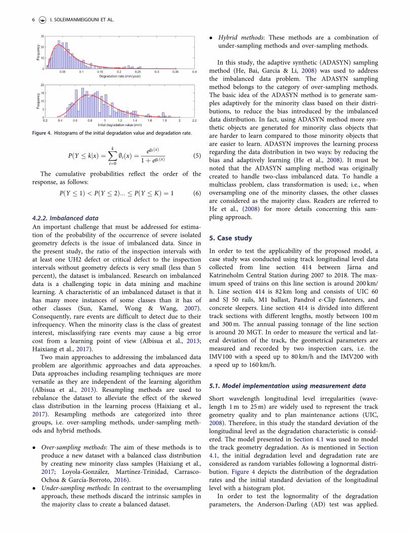
Short wavelength longitudinal level irregularities (wave-length 1m to 25m) are widely used to represent the trackgeometry quality and to plan maintenance actions (UIC,2008). Therefore, in this study the standard deviation of thelongitudinal level as the degradation characteristic is consid-ered. The model presented in Section 4.1 was used to modelthe track geometry degradation. As is mentioned in Section4.1, the initial degradation level and degradation rate areconsidered as random variables following a lognormal distri-bution. Figure 4 depicts the distribution of the degradationrates and the initial standard deviation of the longitudinallevel with a histogram plot.

In order to test the lognormality of the degradationparameters, the Anderson-Darling (AD) test was applied.

Figure 4. Histograms of the initial degradation value and degradation rate.

6 I. SOLEIMANMEIGOUNI ET AL.

The p-values for the AD tests performed on the initial deg-radation value and degradation rate are 0.35 and 0.14,respectively. Considering the significance level of 0.05, theresults of the tests show that there is no reason to reject thelognormality assumption for the initial degradation valueand degradation rate. The estimated parameters of the log-normal distributions for the initial degradation value anddegradation rate are presented in Table 3.

To construct the tamping recovery model, the followingexplanatory variables were included: (1) Ds tmi, sð Þ, which isthe degradation level before a tamping intervention,(2) x1j, s, which is a dummy variable with value 0 when thejth tamping is a partial tamping performed on section s andvalue 1 when the jth tamping is a complete tamping per-formed on section s, and (3) xð2Þ2, j, s, xð3Þ2, j, s, xð4Þ2, j, s, and xð5Þ2, j, s,which are dummy variables representing the second, third,fourth, and fifth interventions, respectively. The recoverymodel is formulated as follows:

Ri, s ¼ a1 þ b0Ds tmi, sð Þ þ b1x1, j, s þ b2xð2Þ2, j, s þ b3x

ð3Þ2, j, s

þ b4xð4Þ2, j, s þ b5x

ð5Þ2, j, s þ d

(7)

where a1, b0, b1, b2, b3, b4, and b5 are the model coeffi-cients. The estimated parameters of the recovery modelobtained using the least squares algorithm are presented inTable 4.

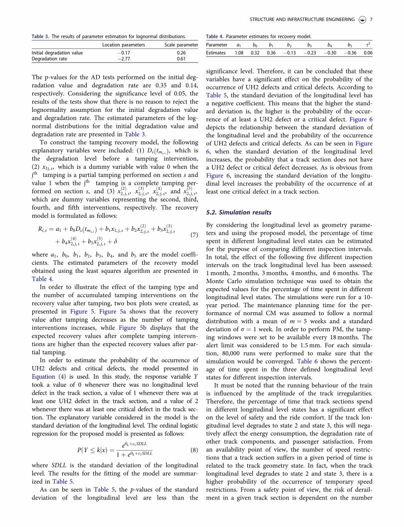
In order to illustrate the effect of the tamping type andthe number of accumulated tamping interventions on therecovery value after tamping, two box plots were created, aspresented in Figure 5. Figure 5a shows that the recoveryvalue after tamping decreases as the number of tampinginterventions increases, while Figure 5b displays that theexpected recovery values after complete tamping interven-tions are higher than the expected recovery values after par-tial tamping.

In order to estimate the probability of the occurrence ofUH2 defects and critical defects, the model presented inEquation (4) is used. In this study, the response variable Ytook a value of 0 whenever there was no longitudinal leveldefect in the track section, a value of 1 whenever there was atleast one UH2 defect in the track section, and a value of 2whenever there was at least one critical defect in the track sec-tion. The explanatory variable considered in the model is thestandard deviation of the longitudinal level. The ordinal logisticregression for the proposed model is presented as follows:

P Y � kjxð Þ ¼ ehkþc1SDLL

1þ ehkþc1SDLL(8)

where SDLL is the standard deviation of the longitudinallevel. The results for the fitting of the model are summar-ized in Table 5.

As can be seen in Table 5, the p-values of the standarddeviation of the longitudinal level are less than the

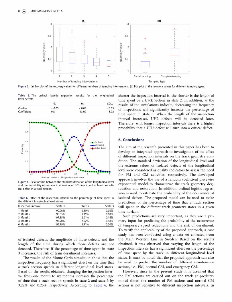
significance level. Therefore, it can be concluded that thesevariables have a significant effect on the probability of theoccurrence of UH2 defects and critical defects. According toTable 5, the standard deviation of the longitudinal level hasa negative coefficient. This means that the higher the stand-ard deviation is, the higher is the probability of the occur-rence of at least a UH2 defect or a critical defect. Figure 6depicts the relationship between the standard deviation ofthe longitudinal level and the probability of the occurrenceof UH2 defects and critical defects. As can be seen in Figure6, when the standard deviation of the longitudinal levelincreases, the probability that a track section does not havea UH2 defect or critical defect decreases. As is obvious fromFigure 6, increasing the standard deviation of the longitu-dinal level increases the probability of the occurrence of atleast one critical defect in a track section.

5.2. Simulation results

By considering the longitudinal level as geometry parame-ters and using the proposed model, the percentage of timespent in different longitudinal level states can be estimatedfor the purpose of comparing different inspection intervals.In total, the effect of the following five different inspectionintervals on the track longitudinal level has been assessed:1month, 2months, 3months, 4months, and 6months. TheMonte Carlo simulation technique was used to obtain theexpected values for the percentage of time spent in differentlongitudinal level states. The simulations were run for a 10-year period. The maintenance planning time for the per-formance of normal CM was assumed to follow a normaldistribution with a mean of m ¼ 5 weeks and a standarddeviation of r ¼ 1 week. In order to perform PM, the tamp-ing windows were set to be available every 18months. Thealert limit was considered to be 1.5mm. For each simula-tion, 80,000 runs were performed to make sure that thesimulation would be converged. Table 6 shows the percent-age of time spent in the three defined longitudinal levelstates for different inspection intervals.

It must be noted that the running behaviour of the trainis influenced by the amplitude of the track irregularities.Therefore, the percentage of time that track sections spendin different longitudinal level states has a significant effecton the level of safety and the ride comfort. If the track lon-gitudinal level degrades to state 2 and state 3, this will nega-tively affect the energy consumption, the degradation rate ofother track components, and passenger satisfaction. Froman availability point of view, the number of speed restric-tions that a track section suffers in a given period of time isrelated to the track geometry state. In fact, when the tracklongitudinal level degrades to state 2 and state 3, there is ahigher probability of the occurrence of temporary speedrestrictions. From a safety point of view, the risk of derail-ment in a given track section is dependent on the number

Table 3. The results of parameter estimation for lognormal distributions.

Location parameters Scale parameter

Initial degradation value �0.17 0.26Degradation rate �2.77 0.61

Table 4. Parameter estimates for recovery model.

Parameter a1 b0 b1 b2 b3 b4 b5 s2

Estimates 1.08 0.32 0.36 �0.13 �0.23 �0.30 �0.36 0.06

STRUCTURE AND INFRASTRUCTURE ENGINEERING 7

of isolated defects, the amplitude of those defects, and thelength of the time during which those defects are notdetected. Therefore, if the percentage of time spent in state3 increases, the risk of train derailment increases.

The results of the Monte Carlo simulation show that theinspection frequency has a significant effect on the time thata track section spends in different longitudinal level states.Based on the results obtained, changing the inspection inter-val from one month to six months increases the percentageof time that a track section spends in state 2 and state 3 by3.22% and 0.25%, respectively. According to Table 6, the

shorter the inspection interval is, the shorter is the length oftime spent by a track section in state 2. In addition, as theresults of the simulations indicate, decreasing the frequencyof inspections will significantly increase the percentage oftime spent in state 3. When the length of the inspectioninterval increases, UH2 defects will be detected later.Therefore, with longer inspection intervals there is a higherprobability that a UH2 defect will turn into a critical defect.

6. Conclusions

The aim of the research presented in this paper has been todevelop an integrated approach to investigation of the effectof different inspection intervals on the track geometry con-dition. The standard deviation of the longitudinal level andthe extreme values of isolated defects of the longitudinallevel were considered as quality indicators to assess the needfor PM and CM activities, respectively. The developedapproach involves the use of a random coefficient piecewiseexponential model to characterize the track geometry deg-radation and restoration. In addition, ordinal logistic regres-sion is used to estimate the probability of the occurrence ofisolated defects. The proposed model can be used to makepredictions of the percentage of time that a track sectionwill spend in the different track geometry states in a giventime horizon.

Such predictions are very important, as they are a pri-mary input for predicting the probability of the occurrenceof temporary speed reductions and the risk of derailment.To verify the applicability of the proposed approach, a casestudy has been conducted using a data set collected fromthe Main Western Line in Sweden. Based on the resultsobtained, it was observed that varying the length of theinspection intervals has a significant effect on the percentageof time spent by the track in different longitudinal levelstates. It must be noted that the proposed approach can alsobe used to predict the number of different maintenanceactions, i.e., PM, normal CM, and emergency CM.

However, since in the present study it is assumed thatthe PM actions are carried out on the track at predeter-mined times, the number of PM actions and normal CMactions is not sensitive to different inspection intervals. In

Figure 5. (a) Box plot of the recovery values for different numbers of tamping interventions, (b) Box plot of the recovery values for different tamping types.

Table 5. The ordinal logistic regression results for the longitudinallevel defects.

h1 h2 SDLL

P-value <0.05 <0.05 <0.05Coefficient 9.8 13.02 �5.02

Figure 6. Relationship between the standard deviation of the longitudinal leveland the probability of no defect, at least one UH2 defect, and at least one crit-ical defect in a track section.

Table 6. Effect of the inspection interval on the percentage of time spent inthe different longitudinal level states.

Inspection interval State 1 State 2 State 3

1 Month 99.26% 0.69% 0.05%2 Months 98.55% 1.35% 0.10%3 Months 97.85% 2.01% 0.14%4 Months 97.20% 2.62% 0.18%6 Months 95.79% 3.91% 0.30%

8 I. SOLEIMANMEIGOUNI ET AL.

the case of a condition-based maintenance policy beingimplemented, the inspection frequency may affect the num-ber of PM actions and normal CM actions. In this case, bydetermining the different direct and indirect costs for pre-ventive tamping actions, normal corrective tamping actions,emergency corrective tamping actions, inspection, derail-ment, and the loss of capacity, the life cycle cost of eachinspection interval can be assessed for the purpose of choos-ing the most effective one.

Acknowledgements

The authors would like to thank Trafikverket, Bana V€ag F€or Framtiden(BVFF), Luleå Railway Research Center (JVTC), and SIMTRACK pro-ject partners for their technical and financial support provided duringthis project.

Disclosure statement

No potential conflict of interest was reported by the authors.

References

Albisua, I., Arbelaitz, O., Gurrutxaga, I., Lasarguren, A., Muguerza, J.,& P�erez, J. M. (2013). The quest for the optimal class distribution:an approach for enhancing the effectiveness of learning via resam-pling methods for imbalanced data sets. Progress in ArtificialIntelligence, 2(1), 45–63. doi:10.1007/s13748-012-0034-6

Andrade, A. R., & Teixeira, P. F. (2013). Unplanned-maintenanceneeds related to rail track geometry. Proceedings of the Institution ofCivil Engineers - Transport, 167(6), 400–410. doi:10.1680/tran.11.00060

Andrews, J., Prescott, D., & De Rozi�eres, F. (2014). A stochastic modelfor railway track asset management. Reliability Engineering &System Safety, 130, 76–84. doi:10.1016/j.ress.2014.04.021

Arasteh Khouy, I., Larsson-Kråik, P., Nissen, A., Juntti, U., &Schunnesson, H. (2014). Optimisation of track geometry inspectioninterval. Proceedings of the Institution of Mechanical Engineers, PartF: Journal of Rail and Rapid Transit, 228(5), 546–556.

AREMA. (2006). Manual for railway engineering (Report No. 4).American Railway Engineering and Maintenance-of-WayAssociation USA.

C�ardenas-Gallo, I., Sarmiento, C. A., Morales, G. A., Bolivar, M. A., &Akhavan-Tabatabaei, R. (2017). An ensemble classifier to predicttrack geometry degradation. Reliability Engineering & System Safety,161, 53–60.

EN 13848–5. (2008). Railway applications – track – track geometryquality – Part 5: Geometric quality levels. Brussels, Belgium: CEN(European Committee for Standardization).

Haixiang, G., Yijing, L., Shang, J., Mingyun, G., Yuanyue, H., & Bing,G. (2017). Learning from class-imbalanced data: review of methodsand applications. Expert Systems with Applications, 73, 220–239.

He, H., Bai, Y., Garcia, E. A., & Li, S. (2008). ADASYN: adaptive syn-thetic sampling approach for imbalanced learning. Paper presentedat 2008 IEEE International Joint Conference on Neural Networks(IEEE World Congress on Computational Intelligence), Hong Kong,China.

Hosmer, D. W., Jr, Lemeshow, S., & Sturdivant, R. X. (2013). Appliedlogistic regression. Hoboken: John Wiley & Sons.

Loyola-Gonz�alez, O., Mart�ınez-Trinidad, J. F., Carrasco-Ochoa, J. A., &Garc�ıa-Borroto, M. (2016). Study of the impact of resampling meth-ods for contrast pattern based classifiers in imbalanced databases.Neurocomputing, 175, 935–947.

Lyngby, N., Hokstad, P., & Vatn, J. (2008). RAMS management of rail-way tracks. In Handbook of performability engineering (pp.1123–1145). London: Springer.

Meier-Hirmer, C., Sourget, F., & Roussignol, M. (2005). Optimisingthe strategy of track maintenance. Paper presented at Advances inSafety and Reliability, proceedings of ESREL 2005-European Safetyand Reliability Conference 2005, Tri City (Gdynia–Sopot–Gda�nsk),Poland.

Osman, M. H. B., Kaewunruen, S., Jack, A., & Sussman, J. (2016).Need and opportunities for a ‘Plan B’ in rail track inspection sched-ules. Procedia Engineering, 161, 264–268.

Quiroga, L. M., & Schnieder, E. (2012). Monte Carlo simulation of rail-way track geometry deterioration and restoration. Proceedings of theInstitution of Mechanical Engineers, Part O: Journal of Risk andReliability, 226(3), 274–282. doi:10.1177/1748006X11418422

Soleimanmeigouni, I., Ahmadi, A., & Kumar, U. (2018). Track geom-etry degradation and maintenance modelling: a review. Proceedingsof the Institution of Mechanical Engineers, Part F: Journal of Railand Rapid Transit, 232(1), 73–102.

Soleimanmeigouni, I., Ahmadi, A., Letot, C., Nissen, A., & Kumar, U.(2016). Cost-based optimization of track geometry inspection. Paperpresented at 11th World Congress of Railway Research, Milan, Italy.

Soleimanmeigouni, I., Xiao, X., Ahmadi, A., Xie, M., Nissen, A., &Kumar, U. (2018). Modelling the evolution of ballasted railway trackgeometry by a two-level piecewise model. Structure andInfrastructure Engineering, 14(1), 33–45.

SS-EN 13848-1: 2004þA1. (2008). Railway applications – track – trackgeometry quality –Part 1 Characterisation of track geometry. Sweden:Swedish Standard Institute.

Sun, Y., Kamel, M. S., Wong, A. K., & Wang, Y. (2007). Cost-sensitiveboosting for classification of imbalanced data. Pattern Recognition,40(12), 3358–3378.

Trafikverket. (2015). Ban€overbyggnad – Spårl€age – Krav vid Byggandeoch Underhåll (Track superstructure – Track geometry –Requirements after renewal and maintenance, in Swedish). TDOK2013:0347 v3.0. Borl€ange, Sweden: Trafikverket.

UIC. (2008). Best practice guide for optimum track geomerty durability.Paris, France: ETF - Railway Technical Publications.

Zaayman, L. (2017). The basic principles of mechanized track mainten-ance (3rd ed.). Bingen am Rhein: PMC Media House. doi:978-3-96245-151-6.

STRUCTURE AND INFRASTRUCTURE ENGINEERING 9