investigation of the potential benefits of optimizing

2020 Building Performance Analysis Conference and

SimBuild co-organized by ASHRAE and IBPSA-USA

INVESTIGATION OF THE POTENTIAL BENEFITS OF OPTIMIZING BUILDING

ELEMENT PLACEMENT USING COMPUTATIONAL FLUID DYNAMICS

Nastaran Shahmansouri 1, Rhys Goldstein 1, Farhad Javid

1, Alex Tessier 1, Simon Breslav 1,

Azam Khan 2

1Autodesk Research, Toronto, Canada 2 Department of Computer Science, University of Toronto, Canada

ABSTRACT

Buildings are responsible for more than one-third of

global energy consumption, motivating the use of

modeling to improve energy efficiency while

maintaining occupant comfort. While conventional

energy models are based on well-mixed zones, we

explore the potential benefits of using high-fidelity

models to optimize the exact placement of building

elements. Specifically, we model a single-room

environment and apply computational fluid dynamics to

compare 36 mechanical configurations of supply and

return vents combined with 9 occupant locations. Results

indicate the same forced-air cooling input may produce

location-specific temperatures and air velocities that

vary significantly depending on the configuration of

building elements.

INTRODUCTION

Building construction and maintenance are responsible

for more than one-third of global energy consumption

and generate, directly and indirectly, nearly 40% of total

CO2 emissions (Al Horr et al. 2017; Sinha, Lennartsson,

and Frostell 2016). Moreover, it has been shown that

indoor environmental conditions and thermal comfort

can hugely impact the health, well-being, and

productivity of occupants (ASHRAE 2009; Al Horr et al.

2016; Mendell et al. 2002). Energy modeling receives

considerable attention as a source of insight toward

improving the energy efficiency of buildings and the

comfort of the people who occupy them, though the

impact and potential of current methods is open to debate

(Mahdavi 2020).

The conventional practice for energy modeling is to use

simplified energy models, where a uniform temperature

is predicted for each zone (Kato 2018). Most building

energy modeling tools are based on the well-mixed zone

air assumption, under which the exact placement of

building elements such as supply and return vents (i.e.

the mechanical configuration), windows and room

partitions (i.e. the architectural configuration), and

furniture (i.e. occupant locations) have little impact on

energy efficiency and occupant comfort. Many of these

elements are simplified or neglected in conventional

models (Kim et al. 2015; Lee 2007). Yet depending on

the mechanical, occupant, and architectural

configurations, the well-mixed assumption may be not

sufficient. A design based on conventional building

energy modeling tools may conceal the potential severity

of a poor overall configuration of elements.

Advancements in simulation techniques and computing

power provide a means to employ more detailed models

in building design processes. An alternative to simplified

energy modeling with the well-mixed zone air

assumption is to combine building energy network

modeling and computational fluid dynamics (CFD)

simulations (Kato 2018). By integrating high-fidelity

CFD simulations into energy modeling practice, airflow and thermal comfort could be predicted for various

positions and times in space. CFD analysis has the

potential to help building design and engineering

professionals understand flow properties over a refined

temporal and spatial grid for different mechanical and

architectural configurations. An outstanding question is,

how much improvement in energy use and comfort could

potentially be gained by shifting toward such high-

fidelity models?

The overarching objective of this research is to

investigate the potential benefits of employing high-

fidelity air flow simulations to plan the exact

configuration of architectural and mechanical elements

as well as the locations of occupants in an indoor

environment. Building upon previous work, numerical

techniques are employed to evaluate thermal comfort,

specifically temperature and velocity variations, in

localized volumes where people mostly occupy. The

study is performed on a simplified indoor environment

consisting of a room with cooling, ventilation, and

window elements. The locations of the supply cooling

vent (called supply) and return vent (called return) are

systematically varied to cover multiple location on

opposite walls of the space. Transient turbulent CFD

analyses are conducted on a total of 36 supply-return

© 2020 ASHRAE (www.ashrae.org) and IBPSA-USA (www.ibpsa.us). For personal use only. Additional reproduction, distribution, or transmission in either print or digital form is not permitted without ASHRAE or IBPSA-USA's prior written permission.

574

configurations, see Figure 1. Predicted temperatures and

airflow velocities are then sampled at 9 locations

representing different possible locations of occupants.

It should be mentioned that this study is envisioned as an

early step in a larger effort toward understanding (1) the

degree to which spatial configurations affect comfort and

energy usage in buildings, and (2) the potential benefits

of incorporating high-fidelity CFD simulation into

energy modeling practice in order to optimize element

placement. Future studies of a similar nature could look

at environments with multiple rooms and circulation

areas, multiple occupants with locations determined by

furniture arrangement, multiple supply/return vents, and

other complicating factors.

RELATED WORK

There has been increasing amount of interest in using

CFD analysis in the field of building design (Kato 2018;

Zhai 2006). The applications of CFD include site

planning, natural ventilation studies, pollution dispersion

and control, the prediction of fire and smoke movement

in a building (Zhai 2006). Additionally, the integration

of CFD and building energy modeling has attracted

attention since it can provide more accurate information

about indoor air quality and energy simulation. CFD has

been used for heat transfer analysis in large areas such as

atria and concert halls as well as smaller areas such a

bedroom (Gilani, Montazeri, and Blocken 2016; Hussain

and Oosthuizen 2012; Moosavi et al. 2014; Perén et al.

2015; Sakai et al. 2008; Stavridou and Prinos 2017; Z. J.

Zhai and Chen 2005). Many studies have focused on

natural ventilation and some studies have examined the

effect of forced-air ventilation. Building CFD modeling

efforts can be classified into two main categories: long

term (for several month of a year) and short term (for less

than an hour) (Kato 2018).

CFD modeling for room environments have been

investigated for different applications and purposes. A

number of studies have employed transient and steady-

state analyses to understand the natural ventilations with

heat sources and compared the results with experimental

data (Al-Sanea, Zedan, and Al-Harbi 2012; Gilani,

Montazeri, and Blocken 2016; Stavridou and Prinos

2017; Yang et al. 2015). These studies provide

information on the effectiveness of CFD simulations and

how to improve the accuracy of simulations for

particular applications. Moreover, studies have been

done on the optimization of indoor air conditioning with

active (HVAC) and passive design elements using CFD

and provided suggestions in this area (Lee 2007). Studies

have been conducted on the methods to employ CFD

modeling for building control applications (Kim et al.

2015). Research has been done on estimating the

allowable air return of an HVAC system that minimizes

energy costs while controlling indoor air quality (Kanaan

2019). Numerical investigations have been conducted on

the impact of exhaust height on energy saving and indoor

air quality for a room with a workstation (Ahmed and

Shian 2017).

This study, by contrast, aims to investigate the impact of

the placement of elements of a mechanical system in

conjunction with elements that are conventionally

considered at different stages of the design process. It is

envisioned as a step toward understanding the full impact

of detailed building geometry on air flow patterns and

ultimately building performance. If the impact is low,

then CFD should arguably continue to be limited to the

specific engineering use cases where it is currently

applied. If the impact is high, then future investigation is

needed to determine the benefit and viability of radically

expanding the use of high-fidelity simulations.

Considering the computational costs of high-fidelity

models, surrogate modeling may make it more feasible

to apply CFD at larger scales than previously possible. It

may allow high-fidelity building simulations and multi-

level optimization to be expanded to include multiple

connected indoor spaces as well as HVAC systems

(Gorissen, Dhaene, and De Turck 2009).

SIMULATION

In this paper, the mechanical configuration refers to the

simplified building with particular combined placements

of supply and return. The occupant location refers to the

locations where the velocity and temperature data have

been evaluated. These locations are assumed to be

representative of small localized volumes occupied most

of the time by an occupant. The combined configuration

refers to a particular location where the velocity and

temperature data have been evaluated in the simplified

building with a specific supply and return configuration.

The simplified building modeled has a forced-air cooling

system, return ventilation, and a window. A wide range

of element placements are tested to investigate the

degree to which spatial configurations affect comfort and

energy use.

Configurations

The modeled building has a width of 4.8 m, a depth of 4

m, and a height of 2.7m. The supply and return are

located in two opposite walls, as shown in Figure 1. The

returns are located in the wall at z = 0, and the supplies

are placed in the wall at z = 4 m. The supplies and returns

are rectangle vents with a fixed width and height of 0.75

m and 0.5 m, respectively. The supply and return of each

configuration are placed in one of the six locations

specified in Table 1. This table reports the locations of

the corner with minimum x and y values.


575

Table 2 tabulates the information for all 36 mechanical

configurations (6 supply × 6 return) and associates each

configuration with an ID. The size and location of the

window are kept fixed; the corner of the window with

minimum values is placed at (x = 0, y = 0.6, z = 1). The

window has a height of 1.5 m and a depth of 2 m. The

velocity and temperature data were obtained and

analyzed for 9 locations, i.e. the occupant locations,

shown in blue in Figure 1. Table 3 presents the position

and ID of these locations. The data was obtained for a

height of 1.7 m, representing the average standing height

of a person.

Figure 1 Schematic of the simplified building. The

center-point of all 6 supply and 6 return locations are

respectively shown in green and red. Temperature and

velocity data are obtained for 9 locations inside the room

at a height of 1.7m shown with blue markers.

Table 1 The locations of the supply and return. The

values show the corner with minimum (x, y) values.

SUPPLY (X, Y, Z) RETURN (X, Y, Z)

(0.425,0.425,4) (0.425,0.425,0)

(0.425,1.775,4) (0.425,1.775,0)

(2.025,0.425,4) (2.025,0.425,0)

(2.025,1.775,4) (2.025,1.775,0)

(3.625,0.425,4) (3.625,0.425,0)

(3.625,1.775,4) (3.625,1.775,0)

Computational fluid dynamics simulation

The motion of air in a room is described by the well-

known Navier-Stokes equations, derived by applying the

conservation laws of mass and momentum to a viscous

fluid. The temperature is obtained from the conservation

of energy equation. Navier-Stokes and energy equations

can be coupled to determine the velocity, pressure, and

temperature of a flow through time in a spatial domain.

In Eulerian description, there is a nonlinear advection

term in both momentum and energy equations which

shows the transport of momentum and energy quantities

due to the bulk motion (velocity) of the fluid. Due to the

nonlinearity of this term, the time-dependent behavior of

a fluid can be chaotic, e.g. turbulent. The turbulent

behavior is observed when the ratio of the inertial energy

to the dissipated viscous energy (defined by Reynolds

number) is > 4,000. Considering the common properties

of HVAC and the buildings, the ventilation flow inside a

building is usually turbulent (Kato 2018).

Table 2 Simulation cases and their representative IDs for architectural configurations: Supply and return values

show the corner with minimum (x, y) values.

ID #

x Supply

(m)

y

Supply

(m)

x Return

(m)

y Return

(m) ID #

x

Supply

(m)

y

Supply

(m)

x Return

(m)

y Return

(m)

MC0 2.025 1.775 2.025 1.775 MC18 3.625 0.425 2.02 1.775

MC1 2.025 1.775 2.025 0.425 MC19 3.625 0.425 2.02 0.425

MC2 2.025 1.775 3.625 1.775 MC20 3.625 0.425 3.625 1.775

MC3 2.025 1.775 3.625 0.425 MC21 3.625 0.425 3.625 0.425

MC4 2.025 1.775 0.425 1.775 MC22 3.625 0.425 0.425 1.775

MC5 2.025 1.775 0.425 0.425 MC23 3.625 0.425 0.425 0.425

MC6 2.025 0.425 2.025 1.775 MC24 0.425 1.775 2.025 1.775

MC7 2.025 0.425 2.025 0.425 MC25 0.425 1.775 2.025 0.425

MC8 2.025 0.425 3.625 1.775 MC26 0.425 1.775 3.625 1.775

MC9 2.025 0.425 3.625 0.425 MC27 0.425 1.775 3.625 0.425

MC10 2.025 0.425 0.425 1.775 MC28 0.425 1.775 0.425 1.775

MC11 2.025 0.425 0.425 0.425 MC29 0.425 1.775 0.425 0.425

MC12 3.625 1.775 2.025 1.775 MC30 0.425 0.425 2.025 1.775

MC13 3.625 1.775 2.025 0.425 MC31 0.425 0.425 2.025 0.425

MC14 3.625 1.775 3.625 1.775 MC32 0.425 0.425 3.625 1.775

MC15 3.625 1.775 3.625 0.425 MC33 0.425 0.425 3.625 0.425

MC16 3.625 1.775 0.425 1.775 MC34 0.425 0.425 0.425 1.775

MC17 3.625 1.775 0.425 0.425 MC35 0.425 0.425 0.425 0.425

z

y x

OL0

OL1

OL2

OL3

OL4

OL5

OL6

OL7

OL8


576

Table 3. ID and locations of the occupant locations.

ID Location (m) ID Location (m)

OL0 (1.25, 1.7, 1) OL5 (3.75, 1.7, 2)

OL1 (2.5, 1.7, 1) OL6 (1.25, 1.7, 3)

OL2 (3.75, 1.7, 1) OL7 (2.5, 1.7, 3)

OL3 (1.25, 1.7, 2) OL8 (3.75, 1.7, 3)

OL4 (2.5, 1.7, 2)

The turbulent flow has fine velocity fluctuations which

require fine space resolution or specific turbulence

models for numerical simulations. To model turbulent

flows, two common treatments are used: introducing

turbulent model equations (Reynolds Averaged Navier-

Stokes Modeling (RANS)), or using small-scale space-

filter (large-eddy simulations) (Calautit, Hughes, and

Nasir 2017; Hussain and Oosthuizen 2012; Kato 2018;

Perén et al. 2015). RANS is a popular treatment method

for CFD simulation of buildings. Here, a k-ε Reynolds

averaged Navier-Stokes modeling (RANS) turbulent

model is used to capture the turbulence effects within the

model (Calautit, Hughes, and Nasir 2017; Hussain and

Oosthuizen 2012). The Buoyancy effects are considered

only in the gravitational term of the equations, i.e. the

Boussinesq approximation is used.

We use OpenFOAM to numerically solve the nonlinear

equations and find the velocity, pressure, and

temperature in the room through time. OpenFOAM is an

open-source solver which uses finite volume

discretization. The PIMPLE algorithm which is a

predictor-corrector iterative technique and combines

semi-implicit methods for pressure linked equations

(SIMPLE) and Pressure Implicit Split Operator (PISO)

algorithms is employed to obtain the solutions.

Simulation and analysis process

The transient turbulent CFD analysis based on finite

volume discretization with an element size of 0.05 m was

conducted. The time step was defined variable to ensure

Courant number is lower than 0.5 in each time step. The

transient analysis simulated the simplified-building for a

duration of 5 minutes. The cool air with a velocity of

0.75 m/s was supplied into the room during the

simulation period. The supply air velocity ensures that

the inside air can be exchanged up to 20 times per hour;

the 5-minute simulation period is selected to make sure

the inside air could be exchanged at least once during

simulation. The cool air and the initial inside air

temperatures respectively were 17 ºC and 27 ºC; the

window was simulated with a constant temperature of 32

ºC. This study intended to investigate a case with

extreme temperature differences, within the acceptable

range of Boussinesq approximation (15 ºC for air)

(Ferziger and Perić 2012), which might not reflect

realistic conditions of commercial buildings. Yet

ASHRAE Fundamentals Handbook section (20.10)

suggests a maximum temperature difference of about 8

ºC between supply and the room for cooling when the air

directs horizontally and from a location near the ceiling

(ASHRAE 2009), which is not far from the assumption

made. We acknowledge the importance of relative

humidity for indoor air quality, however, this study only

focuses on temperature and velocity variations based on

the mechanical configuration and occupant location.

To perform the analysis, a parametric model, called

template, was made in OpenFOAM and employed for

the automation of the simulation process (Weller et al.

1998). Python scripts were developed to set up all

simulation cases from the template folder, automate the

geometry and mesh generations processes, and initiate

the solving procedure of OpenFOAM. In the simulation

process, the results in pre-defined locations for all time

steps were collected and reported in files which were

used for further post-processing done in Python.

ParaView is used for the visualization of 3-dimensional

temperature and velocity fields. (Ahrens, Geveci, Law,

Charles 2005).

RESULTS

Results are presented in two sections. Section 1 mainly focuses on investigating the temperature and velocity

variations, and Section 2 analyzes the relative

placements of supply-return.

Temperature and air velocity predictions

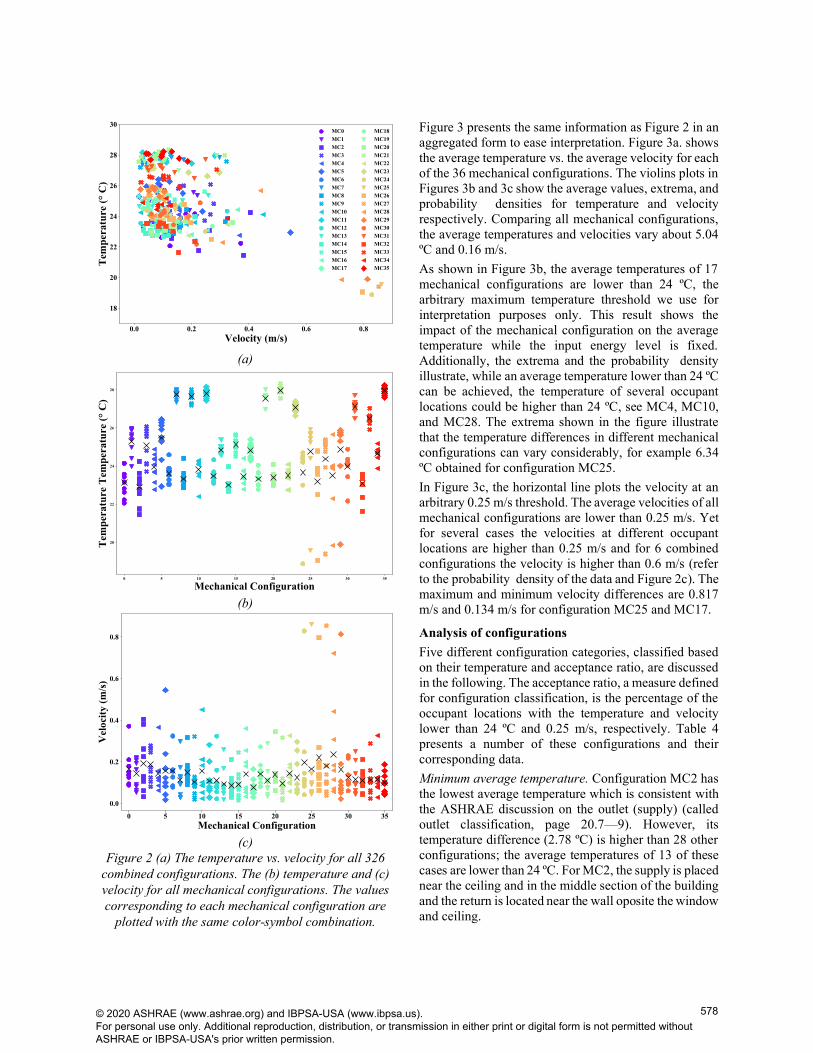
Figure 2 presents the temperature and the velocity values

obtained for all 324 combined configurations (6 supply

× 6 return × 9 occupant locations). The values obtained

for each mechanical configuration, i.e. 9 occupant

locations, are plotted with the same color-symbol

combination. Figure 2a displays the temperature vs.

velocity values; the results indicates that the velocity and

temperature data are mainly clustered in the left-side of

the figure. Yet, a number of combined configurations

with low temperature values have high velocity

(>0.6m/s). For these cases, the cool air with high velocity

flows to the occupant locations which is uncomfortable.

Figure 2b and 2c respectively illustrate the temperature

and velocity values obtained for all combined

configurations. The values corresponding to each

mechanical configuration are plotted vertically. The

average values (over all 9 occupant locations) are also

presented in these plots with black cross-markers for

comparison purpose.


577

(a)

(b)

(c)

Figure 2 (a) The temperature vs. velocity for all 326

combined configurations. The (b) temperature and (c)

velocity for all mechanical configurations. The values

corresponding to each mechanical configuration are

plotted with the same color-symbol combination.

Figure 3 presents the same information as Figure 2 in an

aggregated form to ease interpretation. Figure 3a. shows

the average temperature vs. the average velocity for each

of the 36 mechanical configurations. The violins plots in

Figures 3b and 3c show the average values, extrema, and

probability densities for temperature and velocity

respectively. Comparing all mechanical configurations,

the average temperatures and velocities vary about 5.04

ºC and 0.16 m/s.

As shown in Figure 3b, the average temperatures of 17

mechanical configurations are lower than 24 ºC, the

arbitrary maximum temperature threshold we use for

interpretation purposes only. This result shows the

impact of the mechanical configuration on the average

temperature while the input energy level is fixed.

Additionally, the extrema and the probability density

illustrate, while an average temperature lower than 24 ºC

can be achieved, the temperature of several occupant

locations could be higher than 24 ºC, see MC4, MC10,

and MC28. The extrema shown in the figure illustrate

that the temperature differences in different mechanical

configurations can vary considerably, for example 6.34

ºC obtained for configuration MC25.

In Figure 3c, the horizontal line plots the velocity at an

arbitrary 0.25 m/s threshold. The average velocities of all

mechanical configurations are lower than 0.25 m/s. Yet

for several cases the velocities at different occupant

locations are higher than 0.25 m/s and for 6 combined

configurations the velocity is higher than 0.6 m/s (refer

to the probability density of the data and Figure 2c). The

maximum and minimum velocity differences are 0.817

m/s and 0.134 m/s for configuration MC25 and MC17.

Analysis of configurations

Five different configuration categories, classified based

on their temperature and acceptance ratio, are discussed

in the following. The acceptance ratio, a measure defined

for configuration classification, is the percentage of the

occupant locations with the temperature and velocity

lower than 24 ºC and 0.25 m/s, respectively. Table 4

presents a number of these configurations and their

corresponding data.

Minimum average temperature. Configuration MC2 has

the lowest average temperature which is consistent with

the ASHRAE discussion on the outlet (supply) (called

outlet classification, page 20.7—9). However, its

temperature difference (2.78 ºC) is higher than 28 other

configurations; the average temperatures of 13 of these

cases are lower than 24 ºC. For MC2, the supply is placed

near the ceiling and in the middle section of the building

and the return is located near the wall oposite the window

and ceiling.


578

(a)

(b)

(c)

Figure 3 (a) The variation of average temperature vs.

average velocity of the mechanical configurations. The

average, extrema, and probability density of (b)

temperature and (c) velocity.

High temperature and velocity acceptance ratios (≥89%). For all the cases, the return is placed near the

ceiling yet the supplies are located near the floor or the

ceiling. Both the return and supply are not located near

the window (MC6, MC8, MC12, MC18, and MC20).

High average temperature (≥ 26℃). For all these cases,

the temperature acceptance ratio is 0% and both the

supply and return are located near the floor in different

horizontal locations, which means cool air enters and

exits the room while moving near the floor without being

very well mixed with the warm air (MC7, MC9, MC19,

MC21, MC23, MC33, and MC35). The results are

consistent with ASHRAE suggestions that a supply

located near the floor which direct the flow horizontally

into the room are not recommended for summer cooling

(page 20.11). A large stagnant zone could be formed in

the entire upper region of the room.

Table 4 Information on the mechanical of

configurations with the minimum and maximum

average temperatures, low and high thermal

acceptance ratio, and high temperature variation. In

the table, Conf = configuration, Ave=average,

Accep=Acceptance ratio.

Conf

Sch

em

Ave

T

Tem

p

ST

DE

Ave

U

Acc

ep

T %

Acc

ep

U %

Minimum average temperature

2 22.9 0.8 0.19 89 67

Maximum average temperature

21 28.0 0.2 0.10 0 89

High acceptance ratio

14 23.0 0.4 0.085 100 100

32 23.1 0.6 0.109 100 100

Low acceptance ratio

23 27.1 0.2 0.126 0 78

9 27.7 0.2 0.103 0 88

Configurations with high temperature variation

24 23.7 1.7 0.199 22 89

29 24.9 1.8 0.165 11 89


579

High temperature variation (around 6℃). For all the

cases, the supply is placed near the window and the

ceiling while the return can be located in all 6 defined

positions for the return (MC24 to MC29). This finding is

not in agreement with the ASHRAE suggestion to direct

cool air toward the heat source (page 20.10).

Summarizing observations on the various categories of

configurations, the relative locations and distances of

supply with respect to the window and return, as well as

supply and return heights, play important roles in

temperature and velocity variations and their averaged

values.

Figure 4 illustrates 3-dimensional representations of

configurations MC2 and MC21, respectively, with the

minimum and maximum average temperatures. The

background room color shows the air temperature and

the streamlines show the airflow patterns and speed. The

streamlines shown in the picture start from a horizontal

line in the inlets. Their purpose is to show the airflow

patterns and mixtures in the room.

(a)

(b)

Figure 4 (a) Configuration MC2 with the minimum

average temperature. (b) Configuration MC21 with the

maximum average temperature. Background room

color shows the air temperature, where red represents

warmer areas, and the streamlines show the airflow

direction and speed.

DISCUSSION

This research considers the possibility of increasing

energy efficiency and enhancing occupant comfort

through architectural, interior, and mechanical system

design decisions collectively informed by high-fidelity

simulations. The results obtained show how mechanical

configurations affect the temperature and velocity

variations through an indoor space. The results indicate

the same forced-air cooling input may produce location-

specific temperatures and velocity that differ by as much

as 9.4 ºC and 0.71 m/s depending on the overall

configuration. Additionally, the average temperature and

velocity may vary about 5.0 ºC and 0.16 m/s depending

on the mechanical configuration.

As stated at the outset, most building energy modeling

tools are based on the well-mixed zone air assumption.

This means the exact placement of building elements

such as supply and return vents, windows, room

partitions, and furniture, have little impact on energy

efficiency and occupant comfort, and are therefore

simplified or neglected in conventional models. The

results of this study show that average values are not

always good representatives of the thermal and velocity

characteristics of a space. Depending on the building, it

is possible that a reliance on the well-mixed assumption may obscure opportunities to improve the configuration

building elements in a way that appreciably improves

energy efficiency or comfort.

Further investigation of element placements for different

configurations reveal interesting points. The results for

MC14 is surprising because the supply and the return of

this configuration are directly facing each other, which

means this design might not be the primary configuration

that a designer considers. Additionally, for all cases with

high acceptance ratios (≥ 89%), the return is placed near

the ceiling yet the supplies are located near the floor or

the ceiling; as mentioned above, while the return location

is in agreement with ASHRAE guidelines, the supply

location does not follow the recommendations about

placing the supply near the floor. For these cases, the

return and supply are not located near the heat source,

i.e. the window. Additionally, for all cases with high

temperature variations (around 6), the supply is placed

near the window and the ceiling, which is not consistent

with ASHRAE’s recommendations about supply

placement as discussed before; the return is located in all

6 pre-defined positions. While the results for a number

of cases are in agreement with ASHRAE’s guidelines on

supply and return locations, the findings suggest that

temperature and velocity variations are complex

functions of relative element placement and need deeper

examination. It should be noted that the performance


580

analysis provided by ASHRAE (section 20) is mainly

based on airflow patterns (ASHRAE 2009).

This study is a step toward exploring the possible range

of effects the architectural, occupant, and combined

configurations can have on energy efficiency and

occupant comfort. Further investigation on the temporal

data at occupant locations could reveal new aspects of

design and comfort. Moreover, an important aspect for

building design is their resilience and adaptiveness to

changes as occupants continuously interact with

buildings. The system energy consumption and life-

cycle costs are functions of these interactions and

changes. Optimizing and controlling the temperature and

the velocity locally, where occupants spend most of their

time, might result in lower energy use. High-fidelity

CFD analyses could provide means to better manage and

control buildings under these changes. The direction of

the airflow, air temperature, and air speed are among

other CFD parameters which could be controlled and

adjusted in a smart building based on occupant locations

and their interactions with the building. To develop a full

picture of the problem, additional studies will be needed

to establish the viability of combining HVAC and CFD

analyses for improving occupant comfort and reducing

energy consumption of build environments; the topic has

been receiving attention (Berquist et al. 2017; Kato

2018; Zhai and Chen 2005).

This work only offers limited aspects of thermal comfort

analysis. For the sake of simplicity, the placement of

thermostats and the building automation system have

been excluded. Whereas the study showed large

discrepancies in temperature, a more comprehensive

model might instead predict large discrepancies in

energy consumption as the system strives to meet a

setpoint. This study also uses simplified assumptions for

the boundary conditions and numerical modeling. For

example, only one air velocity was used at the supply.

The effect of assumptions and parameters of the CFD

simulation and how to improve the simulation accuracy

for particular applications need to be further

investigated. This research has tried to isolate the effects

of temperature and velocity variations due to element

placements, throughout the space. The comparisons of

the results with indices aggregating different data types,

for example Dry Radiant Temperature, may reveal

interesting information for designers (Levermore 2000).

These indices summarize information and could be

practical for designers. Finally, a limited number of

architectural configurations have been examined.

Exploring the effect of radiation and heat conduction

through the walls using conjugate heat transfer models

will also provide more information and could clarify

more aspects of this complex problem. The aim of this

investigation is to provide insight about the potential

effect of combined configurations on the energy and

comfort levels.

CONCLUSION

This research examines to what extent designers and

engineers could save energy and improve comfort by

employing high-fidelity CFD simulations when planning

the arrangement of building elements. By simulating 36

configurations of forced-air cooling supply and return

vents, and extracting predictions at 9 possible occupant

locations, the study shows how element placement can

affect the temperatures and air velocities experienced by

building occupants. Although most building energy

modeling tools are based on the well-mixed zone air

assumption, under which the exact placement of

combined configuration elements have little impact on

energy efficiency and occupant comfort, the results

obtained clarify that the mechanical configuration is

significant, and that the temperature and velocity of one

occupant location is not necessarily representative of a

space’s thermal characteristics. In particular, the results

show that the relative locations and distances of supply

with respect to the window and return as well as supply

and return heights play important roles in temperature

and velocity variations and their averaged values.

Further sensitivity studies, which take the effects of the

placement and size of elements into account, could

provide more insight for designing highly energy

efficient and comfortable buildings. Also, future work is

needed to determine the technological requirements and

viability of incorporating CFD and other high-fidelity

analyses into earlier stages of the design process, so that

all aspects of a design can be simultaneously optimized

with knowledge of the resulting air flow patterns and

their implications.

REFERENCES

Ahmed, AQ, and Shian G. 2017. “Numerical

Investigation of Height Impact of Local Exhaust

Combined with an Office Work Station on Energy

Saving and Indoor Environment.” Building and

Environment 122: 194–205.

Al-Sanea, SA, MF Zedan, and MB Al-Harbi. 2012.

“Effect of Supply Reynolds Number and Room

Aspect Ratio on Flow and Ceiling Heat-Transfer

Coefficient for Mixing Ventilation.” International

Journal of Thermal Sciences 54: 176–87.

Ahrens, J, Geveci, B, Law, C, “ParaView: An End-User

Tool for Large Data Visualization, Visualization

Handbook”, Elsevier, 2005

ASHRAE. 2009. “ASHRAE Handbook of

Fundamentals.” New York. The American Society

of Heating, Refrigerating and Air-Conditioning

Engineers.


581

Berquist, J, Tessier, A, O'Brien, W, Attar, R, and Khan,

A. 2017. “An Investigation of Generative Design

for Heating, Ventilation, and Air-Conditioning.”

Proceedings of the Symposium on Simulation for

Architecture and Urban Design. Society for

Computer Simulation International.

Calautit, JK, Hughes, BR, and Nasir DS. 2017. “Climatic

Analysis of a Passive Cooling Technology for the

Built Environment in Hot Countries.” Applied

Energy 186: 321–35.

Ferziger, JH, and Perić, M. 2012. Computational

Methods for Fluid Dynamics. Berlin: Springer

International Publishing.

Gilani, S., Montazeri H., and Blocken B. 2016. “CFD

Simulation of Stratified Indoor Environment in

Displacement Ventilation: Validation and

Sensitivity Analysis.” Building and Environment

95: 299–313.

Al Horr, Y, Arif, M, Kaushik, A, Mazroei, A,

Katafygiotou, M, and Elsarrag, E. 2016.

“Occupant Productivity and Office Indoor

Environment Quality: A Review of the Literature.”

Building and environment, 105: 369–89.

Al Horr, Y, Arif, M, Kaushik, A, Mazroei, A, Elsarrag,

E, and Mishra, S. 2017. “Occupant Productivity

and Indoor Environment Quality: A Case of

GSAS.” International Journal of Sustainable Built

Environment 6(2): 476–90.

Gorissen, D, Dhaene, T, and De Turck, F, 2009.

“Evolutionary model type selection for global

surrogate modeling.” Journal of Machine

Learning Research, 10(71): 2039-2078.

Hussain, S, and Oosthuizen PH. 2012. “Numerical Study

of Buoyancy-Driven Natural Ventilation in a

Simple Three-Storey Atrium Building.”

International Journal of Sustainable Built

Environment 1(2): 141–57.

Kanaan, M. 2019. “CFD Optimization of Return Air

Ratio and Use of Upper Room UVGI in Combined

HVAC and Heat Recovery System.” Case Studies

in Thermal Engineering 15: 100535.

Kato, Shinsuke. 2018. “Review of Airflow and

Transport Analysis in Building Using CFD and

Network Model.” Japan Architectural Review

1(3): 299–309.

Kim, D, Braun, JE, Cliff, EM, and Borggaard, JT. 2015.

“Development, Validation and Application of a

Coupled Reduced-Order CFD Model for Building

Control Applications.” Building and Environment

93: 97–111.

Lee, JH. 2007. “Optimization of Indoor Climate

Conditioning with Passive and Active Methods

Using GA and CFD.” Building and environment

42(9): 3333–40.

Levermore, GJ. 2000. “Building energy management

systems: an application to heating and control.”

Taylor & Francis.

Mahdavi, A. 2020. “In the Matter of Simulation and

Buildings: Some Critical Reflections.” Journal of

Building Performance Simulation 13(1): 26–33.

Mendell, MJ, Fisk, WJ, Kreiss, K, Levin, H, Alexander,

D, Cain, WS, Girman, JR, Hines, CJ, Jensen, PA,

Milton, DK and Rexroat, LP. 2002. “Improving

the Health of Workers in Indoor Environments:

Priority Research Needs for a National

Occupational Research Agenda.” American

journal of public health 92(9): 1430–40.

Moosavi, L, Mahyuddin, N, Ab Ghafar, N, and Ismail,

MA. 2014. “Thermal Performance of Atria: An

Overview of Natural Ventilation Effective

Designs.” Renewable and Sustainable Energy

Reviews 34: 654–70.

Perén, JI, van Hooff, T, Leite BC, and Blocken B. 2015.

“CFD Analysis of Cross-Ventilation of a Generic

Isolated Building with Asymmetric Opening

Positions: Impact of Roof Angle and Opening

Location.” Building and Environment 85(0): 263–

76.

Sakai, K, Kubo, R, Kajiya, R, Iwamoto, S, Kurabuchi, T,

and Kishida, T. 2008. “CFD Analysis of Thermal

Environment of a Room with Floor Heating or Air

Conditioning.” Indoor Air 2008, 17-22 August

2008, Copenhagen, Denmark - Paper ID: 315

CFD (August): 17–22.

Sinha R, Lennartsson M, Frostell B. 2016.

“Environmental Footprint Assessment of Building

Structures: A Comparative Study.” Building and

Environment 104: 162–71.

Stavridou, AD, and Prinos PE. 2017. “Unsteady CFD

Simulation Ina Natural Ventilated Room with a

Localized Heat Source.” Procedia environmental

sciences 38: 322–30.

Weller, HG, Tabor G, Jasak H, and Fureby C. 1998. “A

Tensorial Approach to Computational Continuum

Mechanics Using Object-Oriented Techniques.”

Computers in physics 12(6): 620–31.

Yang, X, Zhong, K, Kang, Y, and Tao, T. 2015.

“Numerical Investigation on the Airflow

Characteristics and Thermal Comfort in

Buoyancy-Driven Natural Ventilation Rooms.”

Energy and Buildings 109: 255–66.

Zhai, Z. 2006. “Application of Computational Fluid

Dynamics in Building Design: Aspects and

Trends.” Indoor and Built Environment 15(4):

305–13.

Zhai, ZJ, and Chen, QY. 2005. “Performance of Coupled

Building Energy and CFD Simulations.” Energy

and Buildings 37(4): 333–4


582


583

investigation of the potential benefits of optimizing

Documents