investigation of the refinement of · 2019-02-21 · and the hand calculations prescribed by aisc...
TRANSCRIPT

AN EXPERIMENTAL AND ANALYTICAL INVESTIGATION OF FLOOR VIBRATIONS
By
Steven R. Alvis
Thesis submitted to the faculty of the Virginia Polytechnic Institute and State University
For the partial fulfillment of the degree of
MASTER OF SCIENCE
in
Civil Engineering
APPROVED:
______________________________ THOMAS M. MURRAY, CHAIRMAN
_________________ _ _______________ Raymond H. Plaut Mehdi Setareh
APRIL 2001
BLACKSBURG, VA
Keywords: Structural Engineering, Floor Vibrations, Civil Engineering
AN EXPERIMENTAL AND ANALYTICAL INVESTIGATION OF
FLOOR VIBRATIONS
by
Steven R. Alvis
Thomas M. Murray, Chairman
Civil Engineering
(ABSTRACT)
Several areas of research regarding floor vibrations were studied during the process
of this research. A basic literature review of previous work in the field of floor vibrations
is presented along with a summary of the study.
The first area of study involved a comparison of finite element models with field
tests for a suspended floor system. The suspended floor system underwent several retrofits
to determine which retrofit reduced annoying vibrations the most. Comparisons were also
made to see how well a finite element model could be used to predict the effectiveness of
the retrofits. The attempt to make accurate finite element models was successful.
The second area of study involved an experimental modal analysis (EMA). The
experimental mode shape was compared with that from the finite element model (FEM).
The research done in this area of study also involved measuring damping for a suspended
floor system. The floor system was also subjected to a known input force and the response
of the system was compared to the theoretical response based on the finite element model
and the hand calculations prescribed by AISC Design Guide 11�Floor Vibrations Due to
Human Activity (Murray et al., 1997). The findings helped provide useful information for
the third area of study.
The third area of this study focused on finding a method for performing a quick and
inexpensive field test on a floor system to determine its acceptability. No good method
found.
The fourth area of this study was to find a way to accurately model complex floor
systems with finite element modeling programs. Previous research yielded good results in

-iii-
the area of frequency prediction. However, the main focus of this study was to find a way
to accurately predict peak acceleration of a complex floor system. This portion of research
did not find a way to model complex floor systems in a finite element program for
producing accurate peak accelerations. However, the source of error between the finite
element program and the hand calculations was accurately defined.

-iv-
ACKNOWLEDGEMENTS
I�d like to thank my committee members for their support and advice. Dr. Murray
has been a great source of help in my process of learning, research, writing, and especially
editing. The staff at Virginia Tech has been great to work with and learn from as well. I
would also like to recognize the great lab technicians Brett, Dennis, and Ricky. They have
helped me a lot in setting up my tests and helping me with things that I could not even do
by myself with an unlimited amount of time. I would also like to thank Joe Howard for
helping me with my experimental modal analysis testing and for briefing me on the theory
behind the test.
I also thank Nucor Research and Development who sponsored this research.
I also thank all of my fellow classmates here at VT and the many friends whom I
met during my stay here. They have been a great blessing as well. I also thank my
undergraduate professor, Dr. Leftwich, from West Virginia Tech. Without his excellent
instruction I wouldn�t have made it to graduate school. He also talked me into taking a
mechanical vibrations class in my undergraduate level, which helped me get a good start in
this enjoyable field of research.
Special thanks goes to my parents and sister for being there and keeping in touch
and being home when I visit. Also to dad especially who helped with a lot of other things.
Finally and most of all, I would like to thank the Lord Jesus Christ for finding and
saving me while I was at VT. I am not the same person as I was when I came to Tech
because of Him. He is the One who has provided the most support. Also I thank my
brothers and sisters in Christ. God bless you all.

-v-
TABLE OF CONTENTS
ABSTRACT..................................................................................................... II
ACKNOWLEDGEMENTS ..........................................................................IV
TABLE OF CONTENTS ............................................................................... V
LIST OF FIGURES................................................................................... VIII
LIST OF TABLES....................................................................................... XII
CHAPTER I - FLOOR VIBRATIONS: INTRODUCTION AND
LITERATURE REVIEW......................................................................... 1
1.1 INTRODUCTION ..........................................................................................1
1.2 SCOPE OF RESEARCH ................................................................................2
1.3 TERMINOLOGY ...........................................................................................3
1.4 LITERATURE REVIEW ...............................................................................5
1.6 NEED FOR RESEARCH .............................................................................12
CHAPTER II - COMPARING FINITE ELEMENT MODELS TO
TEST DATA ............................................................................................ 14
2.1 INTRODUCTION ........................................................................................14
2.2 CANTILEVER STAIRCASE.......................................................................14
2.3 VIRGINIA TECH LAB FLOOR..................................................................17
2.3.1 Test information................................................................................... 17
2.3.2 Test Configuration 1 ............................................................................ 21
2.3.3 Test Configuration 2 ............................................................................ 22
2.3.4 Test Configuration 3 ............................................................................ 25
2.3.5 Test Configuration 4 ............................................................................ 26
2.3.6 Test Configuration 5 ............................................................................ 27
2.3.7 Test Configuration 6 ............................................................................ 29
2.3.8 Test Configuration 7 ............................................................................ 30
2.3.9 Test Configuration 8 ............................................................................ 32
2.3.10 Test Configuration 9 .......................................................................... 33
2.4 COMMENTS AND CONCLUSIONS .........................................................35

-vi-
CHAPTER III – MATCHING EXCITATIONS OF TEST FLOOR
WITH DESIGN GUIDE ........................................................................ 38
3.1 INTRODUCTION ........................................................................................38
3.2 EXPERIMENTAL SETUP...........................................................................38
3.3 DAMPING COMPARISON.........................................................................39
3.4 MODE SHAPES...........................................................................................42
3.4.1 Introduction and Experimental Procedure ........................................... 42
3.4.2 Sap 2000 Predicted Mode Shapes........................................................ 44
3.4.3 Measured Mode Shapes ....................................................................... 47
3.4.4 Summary and Comparison................................................................... 49
3.5 ACCELERATION DUE TO SINUSOIDAL EXCITATION ......................50
3.5.1 Introduction.......................................................................................... 50
3.5.2 Design Guide Prediction ...................................................................... 50
3.5.3 SAP 2000 Prediction............................................................................ 51
3.5.4 Measured Data ..................................................................................... 51
3.5.6 Summary and Comparison................................................................... 52
3.6 CONCLUSIONS AND COMMENTS .........................................................52
CHAPTER IV - EVALUATION OF FLOOR SYSTEMS BY FIELD
ANALYSIS............................................................................................... 54
4.1 INTRODUCTION ........................................................................................54
4.2 DATA ANALYSIS.......................................................................................54
4.3 CONCLUSIONS, SUMMARY, AND RECOMMENDATIONS................59
CHAPTER V - PREDICTION OF ACCELERATION FOR
COMPLEX FRAMING USING THE DESIGN GUIDE
EXCITATION ......................................................................................... 61
5.1 INTRODUCTION ........................................................................................61
5.2 SAP 2000 VERIFICATION .........................................................................61
5.3 MESH REFINEMENT .................................................................................67
5.4 EFFECTIVE SLAB WIDTH OF FOOTBRIDGE .......................................71
5.5 MULTIPLE BEAM SYSTEMS ...................................................................74

-vii-
5.6 MULTIPLE BAY SYSTEM.........................................................................78
5.7 CONCLUSIONS AND SUMMARY OF RESULTS...................................80
CHAPTER VI - CONCLUSIONS AND RECOMMENDATIONS.......... 81
6.1 INTRODUCTION ........................................................................................81
6.2 GENERAL CONCLUSIONS.......................................................................82
6.2.1 Research Area One � The Staircase and Retrofits ............................... 82
6.2.2 Research Area Two � Virginia Tech Lab Floor Experiments ............. 83
6.3.3 Research Area Three � Field Evaluation ............................................. 83
6.3.4 Research Area Four � Missing Link Between AISC and FE Methods 83
6.3 AREAS OF FUTURE RESEARCH.............................................................84
6.3.1 Modeling Considerations ..................................................................... 84
6.3.2 Other Areas of Research ...................................................................... 84
APPENDIX A - CANTILEVER STAIRCASE PLANS.............................. A
APPENDIX B - DESIGN GUIDE CALCULATIONS FOR LAB
FLOOR...................................................................................................... C
APPENDIX C - FRF SPECTRA PLOTS....................................................H
VITA...............................................................................................................EE

-viii-
LIST OF FIGURES
Figure 1.1 � Basic Sine Wave................................................................................................ 4
Figure 1.2 - Modified Reiher-Meister Scale (Band 1996)..................................................... 6
Figure 1.3 � Recommended Peak Accelerations (Allen and Murray 1993) .......................... 8
Figure 1.4 � Heel-Drop Impact and Approximation.............................................................. 9
Figure 1.5 � Slab and Beam FEM (Beavers 1998) .............................................................. 10
Figure 1.6 � Full Joist Model (Beavers 1998) ..................................................................... 10
Figure 2.1 � Measured Heel Drop Acceleration Trace ........................................................ 15
Figure 2.2 � Simulated Heel Drop Acceleration Trace (SAP 2000).................................... 15
Figure 2.3 � FFT Spectra of Acceleration Traces................................................................ 16
Figure 2.4 � Plan of Virginia Tech Lab Floor ..................................................................... 18
Figure 2.5 � 36LH450/300 Joist Details .............................................................................. 18
Figure 2.6 � 36LH500/300 Joist Details (End Joist)............................................................ 19
Figure 2.7 � 36G10N11.0K Joist-Girder Details ................................................................. 19
Figure 2.8 � Post and Beam Locations ................................................................................ 20
Figure 2.9 � TCN 2 Post locations....................................................................................... 22
Figure 2.10 � View of Retrofit Posts at a Distance.............................................................. 23
Figure 2.11 � Close-up of Intermediate Post Connection.................................................... 23
Figure 2.12 � Typical Base of Retrofit Post ........................................................................ 24
Figure 2.13 � TCN 4 Post Locations ................................................................................... 26
Figure 2.14 � TCN 5 Spreader-Beam Locations ................................................................. 27
Figure 2.15 � Typical Picture of Spreader Beam Supported by Post .................................. 28
Figure 2.16 � TCN 6 Spreader-Beam Locations ................................................................. 29
Figure 2.17 � TCN 7 Spreader-Beam Locations ................................................................. 31
Figure 2.18 � TCN 8 Built-up Beam Location .................................................................... 33
Figure 2.19 � Damping Element Cross Section................................................................... 34
Figure 3.1 � Basic Testing Measurement Chain.................................................................. 38
Figure 3.2� Spectrum Response Curve................................................................................ 40
Figure 3.3 � Modified Spectrum Response Curve............................................................... 42
Figure 3.4 � Burst-Chirp Function....................................................................................... 43
Figure 3.5 � Hanning Window Function ............................................................................. 44

-ix-
Figure 3.6 � Finite Element Mesh Grid for Laboratory Floor ............................................. 45
Figure 3.7 � First Mode of Laboratory Floor....................................................................... 45
Figure 3.8 � Second Mode of Laboratory Floor .................................................................. 46
Figure 3.9 � Third Mode of Laboratory Floor ..................................................................... 46
Figure 3.10 �Floor Grid Used for Testing ........................................................................... 47
Figure 3.11 � First Mode ..................................................................................................... 48
Figure 3.12 � Second Mode ................................................................................................. 48
Figure 3.13 � Third Mode.................................................................................................... 49
Figure 3.14 � Acceleration Traces from Sinusoidal Excitation........................................... 51
Figure 4.1 � Peak Acceleration Versus Rating .................................................................... 55
Figure 4.2 � RMS Acceleration Versus Rating ................................................................... 56
Figure 4.3 � Peak Acceleration From Trace Filtered Below 10 Hz Versus Rating............. 57
Figure 4.4 � Peak Acceleration From Trace Filtered Below 18 Hz Versus Rating............. 57
Figure 4.5 � Fundamental Natural Frequency Versus Rating.............................................. 58
Figure 4.6 � Frequency Times Peak Acceleration Versus Rating ....................................... 59
Figure 5.1 � Typical Spring-Mass System........................................................................... 62
Figure 5.2 � SAP2000 Finite Element Model (FEM) of Spring-Mass System ................... 63
Figure 5.3 � Forcing Function F(t) ...................................................................................... 63
Figure 5.4 � Spring-Mass-Damper System.......................................................................... 64
Figure 5.5 � Displacement Trace of Spring-Mass-Damper System .................................... 64
Figure 5.6 � One Shell Element on Each Side of Beam ...................................................... 68
Figure 5.7 �Two Shell Elements on Each Side of Beam..................................................... 68
Figure 5.8 � Fundamental Natural Frequency Versus Number of Shell Elements per Side 69
Figure 5.9 � Deflection Due to Self-Weight Versus Number of Shell Elements per Side .. 70
Figure 5.10 � Deflection Due to Point Load Versus Number of Shell Elements per Side.. 70
Figure 5.11 � Typical Cross-Section of Footbridge and FEM............................................. 73
Figure 5.12 � Difference Plots for 32 ft Beam System........................................................ 73
Figure 5.13 � Difference Plots for 50 ft Beam System........................................................ 74
Figure 5.14 � Typical Mode Shape for the Fundamental Natural Frequency ..................... 76
Figure 5.15 - Acceleration for System Versus Number of 50 ft Beams .............................. 77
Figure 5.16 � Acceleration for System Versus Number of 25 ft Beams ............................. 77

-x-
Figure A.1 � Plan View of Staircase..................................................................................... A
Figure A.2 � Elevation View of Staircase .............................................................................B
Figure C.1 � FRF Spectrum from Ambient Excitation for TCN 1 ....................................... H
Figure C.2 � FRF Spectrum for Heel Drop Excitation for TCN 1 ....................................... H
Figure C.3 � FRF Spectrum for Walking Parallel Excitation for TCN 1 ............................... I
Figure C.4 � FRF Spectrum for Walking Perpendicular Excitation for TCN 1 ..................... I
Figure C.5 � FRF Spectrum for Bouncing Excitation for TCN 1...........................................J
Figure C.6 � FRF Spectrum for Ambient Excitation for TCN 2 ............................................J
Figure C.7 � FRF Spectrum for Heel Drop Excitation for TCN 2 ....................................... K
Figure C.8 � FRF Spectrum for Walking Parallel Excitation for TCN 2 ............................. K
Figure C.9 � FRF Spectrum for Walking Perpendicular Excitation for TCN 2 ....................L
Figure C.10 � FRF Spectrum for Bouncing Excitation for TCN 2........................................L
Figure C.11 � FRF Spectrum for Ambient Excitation for TCN 3 ........................................M
Figure C.12 � FRF Spectrum for Heel Drop Excitation for TCN 3 .....................................M
Figure C.13 � FRF Spectrum for Walking Parallel Excitation for TCN 3 ........................... N
Figure C.14 � FRF Spectrum for Walking Perpendicular Excitation for TCN 3 ................. N
Figure C.15 � FRF Spectrum for Bouncing Excitation for TCN 3....................................... O
Figure C.16 � FRF Spectrum for Ambient Excitation for TCN 4 ........................................ O
Figure C.17 � FRF Spectrum for Heel Drop Excitation for TCN 4 ...................................... P
Figure C.18 � FRF Spectrum for Walking Parallel Excitation for TCN 4 ............................ P
Figure C.19 � FRF Spectrum for Walking Perpendicular Excitation for TCN 4 ................. Q
Figure C.20 � FRF Spectrum for Bouncing Excitation for TCN 4....................................... Q
Figure C.21 � FRF Spectrum for Ambient Excitation for TCN 5 .........................................R
Figure C.22 � FRF Spectrum for Heel Drop Excitation for TCN 5 ......................................R
Figure C.23 � FRF Spectrum for Walking Parallel Excitation for TCN 5 ............................ S
Figure C.24 � FRF Spectrum for Walking Perpendicular Excitation for TCN 5 .................. S
Figure C.25 � FRF Spectrum for Bouncing Excitation for TCN 5........................................T
Figure C.26 � FRF Spectrum for Ambient Excitation for TCN 6 .........................................T
Figure C.27 � FRF Spectrum for Heel Drop Excitation for TCN 6 ..................................... U
Figure C.28 � FRF Spectrum for Walking Parallel Excitation for TCN 6 ........................... U
Figure C.29 � FRF Spectrum for Walking Perpendicular Excitation for TCN 6 ................. V

-xi-
Figure C.30 � FRF Spectrum for Bouncing Excitation for TCN 6....................................... V
Figure C.31 � FRF Spectrum for Ambient Excitation for TCN 7 ........................................W
Figure C.32 � FRF Spectrum for Heel Drop Excitation for TCN 7 .....................................W
Figure C.33 � FRF Spectrum for Walking Parallel Excitation for TCN 7 ........................... X
Figure C.34 � FRF Spectrum for Walking Perpendicular Excitation for TCN 7 ................. X
Figure C.35 � FRF Spectrum for Bouncing Excitation for TCN 7....................................... Y
Figure C.36 � FRF Spectrum for Ambient Excitation for TCN 8 ........................................ Y
Figure C.37 � FRF Spectrum for Heel Drop Excitation for TCN 8 ......................................Z
Figure C.38 � FRF Spectrum for Walking Parallel Excitation for TCN 8 ............................Z
Figure C.39 � FRF Spectrum for Walking Perpendicular Excitation for TCN 8 ...............AA
Figure C.40 � FRF Spectrum for Bouncing Excitation for TCN 8.....................................AA
Figure C.41 � FRF Spectrum for Ambient Excitation for TCN 9 ...................................... BB
Figure C.42 � FRF Spectrum for Heel Drop Excitation for TCN 9 ................................... BB
Figure C.43 � FRF Spectrum for Walking Parallel Excitation for TCN 9 .........................CC
Figure C.44 � FRF Spectrum for Walking Perpendicular Excitation for TCN 9 ...............CC
Figure C.45 � FRF Spectrum for Bouncing Excitation for TCN 9.....................................DD

-xii-
LIST OF TABLES
Table 2.1 � Test Configuration Summary............................................................................ 20
Table 2.2 � TCN 1 Data Summary ...................................................................................... 21
Table 2.3 � TCN 2 Data Summary ...................................................................................... 25
Table 2.4 � TCN 3 Data Summary ...................................................................................... 25
Table 2.5 � TCN 4 Data Summary ...................................................................................... 27
Table 2.6 � TCN 5 Data Summary ...................................................................................... 28
Table 2.7 � TCN 6 Data Summary ...................................................................................... 30
Table 2.8 � TCN 7 Data Summary ...................................................................................... 31
Table 2.9 � Beam Geometry ................................................................................................ 32
Table 2.10 � TCN 8 Data Summary .................................................................................... 32
Table 2.11 � TCN 9 Data Summary .................................................................................... 34
Table 3.1 � Spectrum Response Data .................................................................................. 40
Table 3.2 � Measured and Predicted Frequencies of Mode Shapes .................................... 49
Table 5.1 � Summary of Beam Fundamental Natural Frequency ....................................... 66
Table 5.2 � Data for Mesh Refinement................................................................................ 69
Table 5.3 � 32 ft Beam Data ................................................................................................ 72
Table 5.4 � 50 ft Beam Data ................................................................................................ 72
Table 5.5 - Modal Contributions......................................................................................... 79

-1-
CHAPTER I
FLOOR VIBRATIONS:
INTRODUCTION AND LITERATURE REVIEW
1.1 INTRODUCTION
Throughout the history of structural engineering, many advances have increased
efficiency of design and construction. Such increases in technology ranging from new
materials, design codes, and construction techniques have allowed the completion of great
monumental structures. Although these advancements may allow completion of
lightweight systems with higher strength than their ancestral predecessors, serviceability
problems can still arise in these more efficient products. A common serviceability issue
that arises is the problem of floor vibrations.
Floor vibrations are a serviceability issue that can occur in a system that is perfectly
sound from a strength standpoint. This issue is primarily caused by the combined use of
lightweight concrete and high-strength materials that are used to fabricate flexible, long-
span floor systems. In extreme cases, issues of floor vibrations can render a facility totally
unusable by the occupants based solely on levels of personal comfort. Accurate prediction
is not an easy goal because of the human-based factor. Everyone has a different tolerance
level based on his or her own idea of personal comfort.
If a system is found to be a �problem-system,� it can be rather expensive to correct.
If a situation arises with only one or two individuals on the floor, relocation of the affected
people closer to a structural support can solve the problem easily. However, if a number of
occupants are annoyed because of a neglected design consideration, a more expensive

-2-
solution will be required. It is much easier and less expensive to design the floor against
such vibrations. If the appropriate design actions are taken, the building owner can save
considerable expense.
Current methods of vibration prediction in floor systems range from hand
calculations of a simplified model to complex finite element models. The variety of
techniques usually yield different results due to the different simplifying assumptions in
each method and because of the general complex nature of the floor vibrations. This study
looks into several aspects of floor vibration to achieve a greater understanding of the
phenomenon in general. This chapter presents the scope of study, related terminology,
background information and history, current research, and the need for research, followed
by a summary of the following chapters.
1.2 SCOPE OF RESEARCH
The general goal of this research is to gain a better understanding of vibration
phenomena in order to apply it to a better prediction than what exists for real systems. This
study includes four main areas of research. The first area involves comparisons between
test data and finite element models of simple systems. Secondly, comparisons are made
between dynamic loading tests on a one-bay system and finite element model results. This
second area of research is an attempt to excite a real system with the specified excitation in
the American Institute of Steel Construction Design Guide 11--Floor Vibrations Due to
Human Activity (1997). These test results are compared with results from a finite element
model using the corresponding dynamic load. The third area of study attempts to find a
good field test that will yield immediate results on the quality of a floor without requiring
expensive testing equipment. Test data taken from several floors around the United States

-3-
are analyzed, compared, evaluated, and ranked. The fourth and final area of this study is to
accurately predict the peak acceleration for complex framing. This portion of the study is
purely analytical and involves the use of finite element models with the Design Guide
excitation force. The following section defines relevant terminology for this area of study.
1.3 TERMINOLOGY
Several definitions of the terminology critical to this study are contained within this
section.
Wave � a disturbance traveling through a medium by which energy is transferred
from one particle of the medium to another without causing any permanent displacement of
the medium itself. In this case the energy input is due to a dynamic force.
Dynamic Force � a force that changes with respect to time (not static).
Vibration � Oscillation of a system in alternately opposite directions from its
position of equilibrium, when that equilibrium position has been disturbed. Two types are
free vibration and forced vibration. Forced vibration takes place when a dynamic force
disturbs equilibrium in the system. Free vibration takes place after the dynamic force
becomes static (or zero).
Amplitude � The offset of equilibrium of the system at a given time. Also known as
the magnitude of the wave when plotting displacement, velocity, or acceleration against
time. (see Figure 1.1).

-4-
TIME
Mag
nitu
de
Figure 1.1 – Basic Sine Wave
Period � The amount of time it takes for one cycle (see Figure 1.1).
Cycle � A complete motion of a system starting at any given point of magnitude and
direction that ends with the same magnitude and direction (i.e., the motion over a full
period).
Frequency � number of cycles over a given time, usually cycles per second (also
called Hz).
Natural Frequency � A frequency at which the system will vibrate freely when
excited by a sudden force.
Fundamental Natural Frequency � the lowest natural frequency for the system at
which a system will vibrate.
Resonance � a condition where a system is excited at one of its natural frequencies.
Damping � a property of energy dissipation within the system. More damping
results in a quicker decay of amplitude in free vibration. When less damping is present, the
system retains its energy for a longer amount of time.
Amplitude
Period

-5-
Viscous Damping � the form of damping that is proportional to velocity. This is the
easiest type of damping to model mathematically.
Fast Fourier Transform (FFT)- An algorithm for computing the Fourier transform
of a set of discrete data values. The FFT expresses the data in terms of its component
frequencies.
FFT Spectrum � The relative contribution of frequencies in a trace of amplitude
over a time range. This is obtained by performing an FFT of the data.
Mode shapes � The shape of a system showing relative displacements when
undergoing vibration.
Node � The point location on a mode shape that undergoes zero relative
displacement.
Anti-node � The point location on a mode shape that undergoes maximum relative
deflection.
Node-line � The line on a mode shape that undergoes zero deflection. Node-lines
occur on surfaces.
1.4 LITERATURE REVIEW
The first known stiffness criterion for floors was proposed by Treadgold (1828).
He indicated that timber beams should be made deeper to reduce the vibration caused by
people moving on the floors of houses. Most of the recent design criteria can be found in
the AISC Steel Design Guide Series 11�Floor Vibrations Due to Human Activity (Murray
et al. 1997). Design criteria are based on levels of human comfort; levels of comfort can
depend on both the environment and the individual.

-6-
Reiher and Meister (1931) did a study to determine exactly what combinations of
frequency and amplitude affect humans. Subjects of the research were placed on shaking
tables and subjected to steady state motion. The frequencies varied from 5 to 70 Hz and
the amplitude ranged from 0.001 to 0.04 in. Classifications of �slightly perceptible�,
�distinctly perceptible�, �strongly perceptible�, �disturbing�, and �very disturbing� were
used to describe the vibration conditions. Lenzen (1966) proposed that the amplitudes of
the Reiher-Meister scale be lowered by a factor of ten to account for the transient nature of
floor vibrations. The Lenzen modified Reiher-Meister scale is shown in Figure 1.2.
Figure 1.2 - Modified Reiher-Meister Scale (Band 1996)
In 1975, Murray suggested �steel beam, concrete slab systems, with relatively open
areas free of partitions and damping between 4 and 10 percent, which plot above the upper
one-half of the distinctly perceptible range, will result in complaints from the occupants�.
Figure 1.2 shows this acceptability criterion and is called the Reiher-Meister/Murray

-7-
criterion. Everything below the dotted line in the figure is considered acceptable by the
criterion.
In 1981, Murray established an acceptability criterion based on the required
damping of a floor system. The required damping is a function of the amplitude of a
system due to a heel-drop impact and its natural frequency. Ninety-one systems with
varying properties were statistically analyzed for Murray (1981) to determine the amount
of damping required for an acceptable system as described in Equation 1.1:
5.235 +> fAD o (1.1)
where D = percent of critical damping, Ao = initial amplitude from a heel-drop impact, in.,
and f = first natural frequency of the floor system, Hz. This equation is valid for systems
with natural frequencies less than 10Hz and spans less than 40ft.
Figure 1.3 is a set of recommended acceleration tolerances for humans (Murray et
al. 1997). It can be seen in this figure how different environments have different
acceptance levels for vibrations.
According to Murray (1991), common values for first natural frequency range
between 5 and 8 Hz. Comfort studies for automobiles and aircraft have found that, in this
range, humans are especially sensitive to the vibration. Murray (1991) explains that this is
due to many of the major organs in the human body resonating at these frequencies. It is
for this reason that the lowest tolerance level is within this frequency range (the flat portion
of the curve).

-8-
Frequency (Hz)
1 3 4 5 8 10 25 40
Peak
Acc
eler
atio
n (%
Gra
vity
)
0.1
0.050.05
0.25
0.5
1
2.5
5
10
25
Rhythmic Activities,Outdoor Footbridges
Indoor Footbridges,Shopping Malls,
Dining and Dancing
Offices,Residences
ISO Baseline Curve for RMS Acceleration
Figure 1.3 – Recommended Peak Accelerations (Allen and Murray 1993)
The primary method for determining the fundamental natural frequency of a floor
system is by hand calculations. Hand calculation methods are found in the AISC Steel
Design Guide Series 11 provisions. Experimental testing and finite element modeling are
two other methods for determining the fundamental natural frequency and frequencies for
higher modes.

-9-
TIME (seconds) 0.00 0.01 0.02 0.03 0.04 0.05
LOA
D (l
bs.)
0
100
200
300
400
500
600
700
MEASURED HEELDROP RESPONSE CURVE
STRAIGHT LINE APPROXIMATION
Figure 1.4 – Heel-Drop Impact and Approximation
Experimental testing is done using an accelerometer and a data collector. The
accelerometer is placed in an area of interest and the floor system is subjected to a dynamic
load. The standard heel drop function is applied to a system by having a 170-lb person
rocking up on the balls of his feet with his heels about 2.5 in. off the floor, and then
relaxing and allowing his heels to impact the floor (Murray 1981). One such loading is a
heel-drop test as measured by Ohmart (1968). He also came up with a reasonably accurate
approximation for the impact as described in Figure 1.4. Other methods of loading the
system include walking in various directions or doing a bounce test. A bounce test is
where a person will try to bounce at a multiple of the natural frequency of the floor system
in an attempt to excite the system at its natural frequency. For all tests,
d
-10-
SLAB CENTROID
RIGID LINK
BEAM CENTROID
Figure 1.5 – Slab and Beam FEM (Beavers 1998)
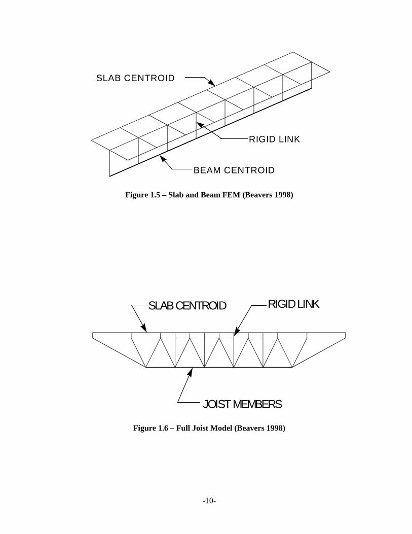
SLAB CENTROID RIGID LINK
JOIST MEMBERS
Figure 1.6 – Full Joist Model (Beavers 1998)

-11-
the dynamic response is measured with the accelerometer and a Fast Fourier Transform
then is used to determine the frequency spectrum.
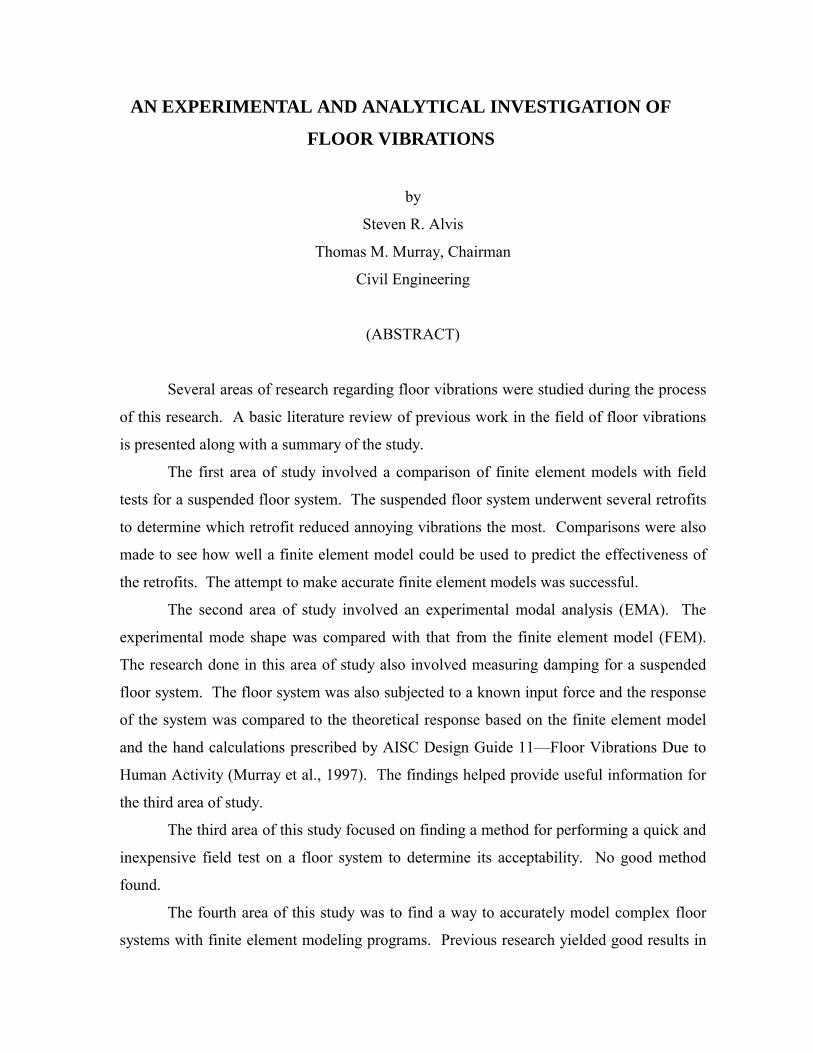
Finite element modeling of floor systems requires several considerations. Figures
1.5 and 1.6 show finite element modeling techniques for steel and concrete composite floor
systems (Beavers 1998). Beavers also determined that, in terms of accuracy and simplicity,
the most efficient way to model a joist girder system is to use at least eight plate elements
for each section of a beam. The work of Gibbings (1993) showed that eccentricities should
be included when modeling joists. The actual eccentricities were not as important as long
as there was eccentricity included in the finite element model (Gibbings 1993). Gibbings
also stated that about 2-in. of eccentricity provides accurate stiffness for joists.
Some of the most recent research which used complex finite element models was
performed by Sladki (1999). This research concluded that the finite element methods gave
a better prediction for the lowest natural frequency of floor systems than the Design Guide
criteria. However, for peak acceleration the analytical methods did not compare well with
the actual test results (Sladki 1999).
Once a floor system has been built and it is found to have poor serviceability due to
excessive vibrations, there are several solutions. Tuned Mass Dampers (TMD) may be
used to reduce vibrations. Research in this area was performed by Rottmann (1996). She
concluded that TMDs could successfully control floor vibrations if there is initially a low
relative damping in the system. She further states that, although it is possible, there are
difficulties in using TMDs to control multiple modes of vibration with closely spaced
frequencies and high damping. Rottmann also noted that the true effectiveness of TMDs is
dependent on the perceptivity of occupants of the structure.

-12-
Another solution to overcome annoying floor vibrations is through active control.
Active control uses an actively controlled mass to dampen vibration (Hanagan 1994).
Hanagan stated that the method is very effective, and it also provides much less disruption
in the building function than most other methods of repair. High initial and maintenance
costs are regarded as serious disadvantages to using this system, according to Hanagan.
1.6 NEED FOR RESEARCH
Different evaluation techniques usually yield different results. The resulting
differences can be due to the different simplifying assumptions in each method and because
of the general complex nature of the floor vibrations. It is under such considerations that
several aspects of floor vibrations and the correlating modeling assumptions should be
studied under greater detail. With greater accuracy of prediction, fewer problems are likely
to arise in completed structures.
The major difficulty for prediction is determining peak acceleration of a floor
system. To predict an accurate peak acceleration, less complex floor systems than those
that were tested in the past were analyzed. A simpler system such as a footbridge or single-
bay system has fewer variables to look at when compared to a complex, multi-bay system.
Thus, there is a higher probability of accurately predicting the peak acceleration.
Chapter II looks at two simple systems. The first system is a cantilever staircase. A
finite element model was made to predict the lowest natural frequency and peak
acceleration of this system. The predictions were compared with actual test data of a heel
drop. The second system is one of several Virginia Tech test floors. This one-bay floor
system underwent various tests. Different excitations were applied to this system. Several

-13-
retrofits were incorporated into the floor to change the vibration characteristics of the
structure. Finite element models were also created to compare the results of the various
tests.
Chapter III contains a discussion of the same laboratory floor subjected to a known
dynamic forcing function. The finite element method, AISC Guide criteria, and the actual
test data are compared. The test data provided information that allowed the measured
system damping, mode shapes, and accelerations to be compared with the finite element
method predictions.
Chapter IV discusses floor vibration data results from several buildings and the
various configurations of the Virginia Tech lab floor. Comparisons were made to
determine if a quick and accurate method of field analysis with only a handheld data
collector and analyzer is possible.
Chapter V looks at the use of the finite element method for the prediction of peak
acceleration for complex framing. The approach in this area of study starts with
comparison of the AISC criteria with the results of the finite element model for a very
simple system. The system complexity was then increased, and an attempt to pinpoint the
source of discrepancies was made. Several techniques were utilized for finding the key
differences between the AISC criteria predictions and those of the finite element model.
Chapter VI presents the conclusions of this study. Also contained in this chapter
are recommendations for future research. Following this last chapter is an Appendix
containing supporting data and drawings.

-14-
CHAPTER II
COMPARING FINITE ELEMENT MODELS TO TEST DATA
2.1 INTRODUCTION
From the review of previous research, it is evident that attempts to predict complex
vibration characteristics have not been entirely successful. SAP2000-Nonlinear finite
element model results were compared to test data obtained in simple, controlled
environments. The first simple model is that of a cantilever staircase. The second model is
the Virginia Tech lab floor with multiple geometric alterations or retrofits. These models
are much more simple than those from previous research and allow a greater probability for
the measurement data sets to match the theoretical values because of fewer system
variables.
2.2 CANTILEVER STAIRCASE
This system is a cantilever staircase located in Doylestown, Pennsylvania. The
member sizes and geometry were obtained from a set of plans courtesy of Marshall Erdman
and Associates, Inc. Simplified details of the staircase are found in Appendix A. A heel
drop was performed on the end of the staircase and the resulting accelerations were
recorded using a handheld FFT analyzer. A simulated heel drop was applied in a finite
element model and the results were compared with the measured staircase response. A
visual comparison between the actual measured trace and that predicted from the finite
element model can be seen in Figures 2.1 and 2.2, respectively. The magnitude of the
simulated trace was scaled for ease of visual comparison with the actual trace. This is valid
because the actual input force for the measured trace can only be assumed. Three percent
modal damping was assumed for the finite element model. The simulated heel drop trace
has less ambient noise present, which is characterized by a smoother wave due to fewer
contributing frequencies in the theoretical model.

-15-
Heel Drop at Edge of Cantilever Staircase
Measured Acceleration Trace
-0.400 -0.300 -0.200 -0.100 0.000 0.100 0.200 0.300 0.400
0 0.5 1 1.5 2 2.5 3 3.5 4 Time (s)
Acce
lera
tion
(g)
Figure 2.1 – Measured Heel Drop Acceleration Trace
Heel Drop at Edge of Cantilever Staircase SAP2000 Simulated Acceleration Trace
-0.400 -0.300 -0.200 -0.100 0.000 0.100 0.200 0.300 0.400
0 0.5 1 1.5 2 2.5 3 3.5 4 Time (s)
Acce
lera
tion
(g)
Figure 2.2 – Simulated Heel Drop Acceleration Trace (SAP 2000)

-16-
Heel Drop at the Edge of Cantilever Staircase
FFT Spectra
7.5
11
0
0.005
0.01
0.015
0.02
0.025
0 5 10 15 20 25 30 35 40 45 50 Frequency (Hz)
Acce
lera
tion
(g)
Measured SAP2000 simulated
Figure 2.3 – FFT Spectra of Acceleration Traces
Figure 2.3 shows direct comparison between the finite element simulation and the
measured heel drop. The curve for the finite element simulation was scaled to obtain a
good graphic comparison. This is a legitimate procedure for two reasons: (1) the input
force was not measured for the actual heel drop, and (2) the primary interest is in the
relative participation of each frequency. Figure 2.3 shows a very crude resemblance
between the simulated curve and the measured curve. Although both have two primary
peaks, the fundamental frequencies are different. The measured fundamental natural
frequency is 7.5 Hz, and the simulated fundamental natural frequency is 11.0 Hz. The
comparison also reveals that the simulated model has less noise. This can be identified by
the smoothness of the curve. Noise spikes are obviously present in the measured data.
Possible sources for these spikes can be from environmental noise, loose connections,
extraneous materials, or a number of other occurrences that are not taken into consideration
by the finite element model.

-17-
2.3 VIRGINIA TECH LAB FLOOR
2.3.1 Test information
The Virginia Tech Lab floor is a suspended floor system supported on four columns
with a concrete deck. The supporting members are 36LH450/300 joists, 36LH500/300
joists, and 36G10N11.0K joist girders as shown in Figure 2.4. The section properties of the
joists and joist girders are shown in Figures 2.5 to 2.7. This laboratory floor had a dual
purpose: (1) to function as a roof for an addition to the Virginia Tech Structures Lab and
(2) to function as a �problem floor� that would be annoying to would-be occupants of an
office building. Hand calculations (using Design Guide criteria) predicted the �problem
floor� to have a natural frequency of 5.88 Hz and a peak acceleration of 2.37% g with 1%
critical damping. (See Appendix B for these calculations.) Several retrofits were
attempted in order to evaluate possible fixes for existing floors.
Nine configurations of the floor were tested. One configuration was the original,
unmodified condition. Retrofit modifications were made for the other eight configurations.
Table 2.1 lists the test configuration number and the corresponding test condition. Figure
2.8 illustrates all of the retrofit locations described in the table. Several types of excitation
were performed on each configuration. Recordings were then made for each type of
excitation: ambient, heel drop, walking perpendicular to joists, walking parallel to joists,
and bouncing. A rating of human comfort level was chosen as well. The floors are ranked
from 1 to 9 on acceptability (1 being the best). The frequency results are described in the
following sections, while the human comfort ranking is discussed in Table 2.1.
The AISC Guideline procedures are only applicable for the unmodified floor and
were used accordingly. SAP 2000 finite element models were made to compare with the
data taken from the accelerometer. The only valid comparison that could be made with one
reading location (in the center of the floor) was to examine the mode shapes and the
corresponding frequencies. The frequencies that corresponded to a mode shape with
vertical motion at the center of the floor were the only ones that are predicted to cause
annoying vibration on the center of the floor.

-18-
36G10N11.0K
30' - 8"
45' - 0" 36LH 450/300
36G10N11.0K
36LH
500
/300
36LH
500
/300
Figure 2.4 – Plan of Virginia Tech Lab Floor
5'-7" 1'-9"
2'-6" 3'-0" 3'-0" 3'-0" 3'-0"
12
34 4
5
4 46
d = 36�
Overhang = 6�
Top Chord = 2L3X3X0.236
Bottom Chord = 2L2.5X2.5X0.22
Web 1 = 2L1.5X1.5X0.15
Web 2 = 1L1.5X1.5X0.129
Web 3 = 2L1.5X1.5X0.129
Web 4 = 1L1.25X1.25X0.118
Web 5 = 1L1.75X1.75X0.15
Web 6 = 1L1.5X1.5X0.15
Cr = 0.8627
Ichords = 1412 in4
Figure 2.5 – 36LH450/300 Joist Details

-19-
5'-7" 1'-9"
2'-6" 3'-0" 3'-0" 3'-0" 3'-0"
1 2
3
2 4
5
6 4
5
d = 36�
Overhang = 6�
Top Chord = 2L3X3X0.33
Bottom Chord = 2L3X3X0.227
Web 1 = 2L1.75X1.75X0.15
Web 2 = 1L1.5X1.5X0.127
Web 3 = 2L1.5X1.5X0.15
Web 4 = 1L1.25X1.25X0.13
Web 5 = 1L1.75X1.75X0.15
Web 6 = 1L1.25X1.25X0.117
Cr = 0.8627
Ichords = 1550 in4
Figure 2.6 – 36LH500/300 Joist Details (End Joist)
2'-7" 1'-9"
1'-3" 3'-0" 3'-0" 3'-0"
12
34 5
4
2 4
d = 36�
Overhang = 6�
Seat = 5�
Top Chord = 2L4X4X0.375
Bottom Chord = 2L4X4X0.375
Web 1 = 2L4X4X0.44
Web 2 = 2L1.5X1.5X0.15
Web 3 = 2L2.5X2.5X0.25
Web 4 = 2L2X2X0.176
Web 5 = 1L2X2X0.176
Cr = 0.7550
Ichords = 3270 in4
Figure 2.7 – 36G10N11.0K Joist-Girder Details

-20-
Table 2.1 – Test Configuration Summary
Test Configuration Number (TCN)
Test Conditions (See Figure 2.5 for Locations)
Comfort Ranking
1 Unmodified 9
2 2 Posts at Location x-2 with bearing pads 2
3 2 Posts at location x-2 with expansion joint material 3
4 Diagonal posts at location x-1 6
5 Posts w/spreader beam at location B (inside of third point) 1
6 Posts w/spreader beam at location A (outside of third point) 7
7 Posts w/spreader beam at location C (diagonal third points) 5
8 Beam at bottom chords of joists along centerline | to joists 8
9 Damping posts at location x-2 4
Figure 2.8 – Post and Beam Locations

-21-
2.3.2 Test Configuration 1
Test Configuration 1 of the Virginia Tech lab floor was the original floor. Table 2.2
shows a summary of the first three frequencies that contribute to annoying vibration in the
center of the lab floor. These frequencies are taken from the peaks of the FRF plots located
in Appendix C. All frequencies that were multiples of the excitation frequency were
ignored unless it was also a natural frequency of the system. For example, if the walking
excitation was 2.25 Hz, the frequencies of 2.25 Hz, 5.50 Hz, 7.75 Hz, etc. were ignored.
However, if one of these multiples happened to match an expected natural frequency, it
was recorded in the table. Thus, the modal frequencies that do not affect the center of the
floor are not looked at for the comparison. This comparison is only to test the effectiveness
of the values predicted by the finite element model. The readings with ambient and heel-
drop excitation were analyzed first to find the frequencies. These gave expected natural
frequencies to look for in the other excitations.
Table 2.2 – TCN 1 Data Summary
Excitation f1
(Hz) f2
(Hz) f3
(Hz)
SAP 2000 Modal Analysis 5.86 9.02 19.56
Ambient 6.00 9.75 19.25
Heel Drop 5.75 9.50 19.00
Walking Parallel 6.00 9.50 19.25
Walking Perpendicular 6.25 9.50 19.00
Bouncing @ 3.75Hz 6.00 9.75 19.25
The AISC Guideline procedure for calculating the fundamental natural frequency of
this floor yields a frequency of 5.88 Hz. This compares quite well with the 5.86 Hz value
obtained from the SAP2000 finite element analysis. The AISC Guideline criterion does not
provide any methods for obtaining higher natural frequencies.
It is obvious that the test data correlated rather well with the predicted values
provided by the finite element analysis. It should be noted that an extra mode with a
frequency of 15.36 Hz was predicted by SAP2000. This prediction is based on the activity
at the center of the floor for the mode shape. However, this modal frequency did not

-22-
appear in any of the measured test data. There is no known explanation for this extra
modal frequency.
2.3.3 Test Configuration 2
Test Configuration 2 incorporates two posts supporting the floor to add stiffness.
The posts are at the third points along the centerline that runs perpendicular to the joists as
seen in Figure 2.9. Elastomeric bearing pads measuring 6in.x6in.x7/8in. were inserted
between the floor and the post to ensure good contact and to possibly add damping. After
the bearing pads were in place, a screw mechanism on top of the post was adjusted to apply
a compressive force. Figures 2.10 to 2.12 show pictures of the posts. The posts were
modeled in SAP2000 as rigid supports restraining motion in the vertical direction. Table
2.3 compares frequencies that contribute to annoying vibration in the center of the floor.
Figure 2.9 – TCN 2 Post locations

-23-
Figure 2.10 – View of Retrofit Posts at a Distance.
Figure 2.11 – Close-up of Intermediate Post Connection

-24-
Figure 2.12 – Typical Base of Retrofit Post
There is no method to accurately predict these frequencies by hand calculations
because of the retrofit. However, it is evident that the SAP 2000 finite element model
analysis predicted these three major contributing frequencies quite well. It is noted that the
finite element model produced slightly higher frequencies. This is due to using a vertically
rigid support for the retrofit posts. If a stiff spring element were used instead, it would
have produced a softer model. This would yield slightly lower frequencies. The 15 Hz
frequency component only appeared in the ambient trace, while the same trace did not
contain the f4 frequency. The f4 frequency prediction also is about 15% higher than the
test data when compared to the other modal frequency components. Overall, it is evident
that there was approximately a 33% increase in the fundamental natural frequency of the
system by this simple retrofit.

-25-
Table 2.3 – TCN 2 Data Summary
Excitation f1
(Hz) f2
(Hz) f3
(Hz) f4
(Hz)
SAP 2000 Modal Analysis 8.91 10.77 15.80-16.20 22.27
Ambient 8.50 10.00 15.00 ---
Heel Drop 8.00 10.00 --- 19.25
Walking Parallel 8-8.5 10.00 --- 19.25-19.5
Walking Perpendicular 8.50 10.50 --- 19.50
Bouncing @ 4.25Hz 8.50 9.75 --- 19.25
2.3.4 Test Configuration 3
The third test configuration is identical to TCN 2 except the elastomeric bearing pad
was replaced with expansion joint material. The expansion joint material used was typical
expansion joint material for concrete slabs. A nine-inch square with a ¼� thickness was
used. Table 2.4 compares frequencies that contribute to annoying vibration in the center of
the floor.
Table 2.4 – TCN 3 Data Summary
Excitation f1
(Hz) f2
(Hz) f3
(Hz)
SAP 2000 Modal Analysis 8.91 10.77 22.27
Ambient 8.25 10.00 19.25
Heel Drop 8.00 10.00 19.50
Walking Parallel
7.75,
8.25 10.00 19.50
Walking Perpendicular 8.25 10.25 19.25
Bouncing @ 4.00Hz 8.00 10.00 19.25
The only notable change from TCN 2 is that the ambient trace contained a 19.25 Hz
peak instead of the 15 Hz peak. The SAP 2000 analysis predicted three frequencies
between 15.80 Hz and 16.20 Hz. The actual test data did not show these frequencies.
-26-
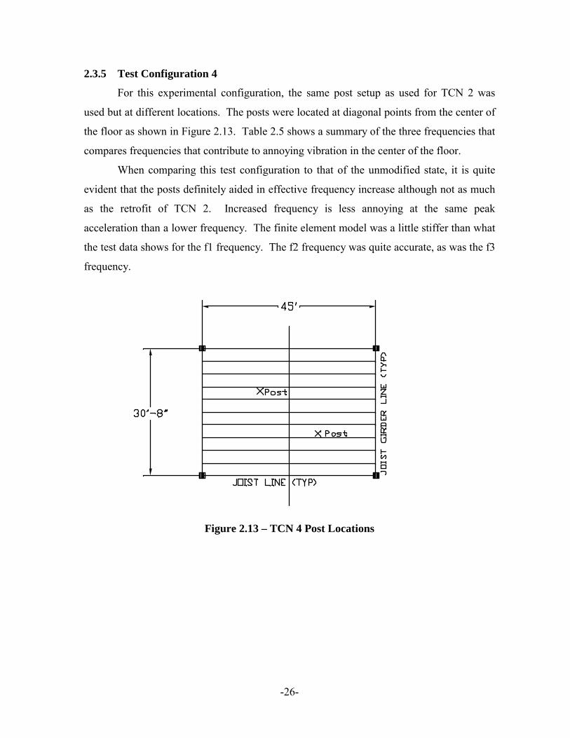
2.3.5 Test Configuration 4
For this experimental configuration, the same post setup as used for TCN 2 was
used but at different locations. The posts were located at diagonal points from the center of
the floor as shown in Figure 2.13. Table 2.5 shows a summary of the three frequencies that
compares frequencies that contribute to annoying vibration in the center of the floor.
When comparing this test configuration to that of the unmodified state, it is quite
evident that the posts definitely aided in effective frequency increase although not as much
as the retrofit of TCN 2. Increased frequency is less annoying at the same peak
acceleration than a lower frequency. The finite element model was a little stiffer than what
the test data shows for the f1 frequency. The f2 frequency was quite accurate, as was the f3
frequency.
Figure 2.13 – TCN 4 Post Locations

-27-
Table 2.5 – TCN 4 Data Summary
Excitation f1
(Hz) f2
(Hz) f3
(Hz)
SAP 2000 Modal Analysis 8.81 9.76 19.12 - 20.49
Ambient 8.00 10.00 19.25
Heel Drop 7.75 9.75 19.25
Walking Parallel 7.75 9.75 20.00
Walking Perpendicular 7.75 10.00 19.00, 20.00
Bouncing @ 4.25Hz 8.00 10.00 19.25
2.3.6 Test Configuration 5
This test configuration used a three-foot-long W6x20 beam centered on the top of
two posts. This spreader beam spanned from the bottom of the top chord of one joist to the
bottom of the top chord of the other joist. The posts were tightened with a screw
mechanism to apply a compressive force. The beams for this fifth configuration are located
as shown in Figure 2.14. Figure 2.15 shows a picture of how the spreader beam is
supported by the post. Table 2.6 shows a comparison of the five frequencies that contribute
to annoying vibration in the center of the floor.
Figure 2.14 – TCN 5 Spreader-Beam Locations

-28-
Table 2.6 – TCN 5 Data Summary
Excitation f1 (Hz)
f2 (Hz)
f3 (Hz)
f4 (Hz)
f5 (Hz)
SAP 2000 Modal Analysis 8.82 12.44 15.37 22.51 24.04
Ambient 8.25-8.75 10.25 12.75 19.50 20.25
Heel Drop 8.25 10.25 -- 19.50 20.50
Walking Parallel 8.00 10.50 -- 19.50 20.50
Walking Perpendicular 8.25 10.50 12.75 19.50 20.50
Bouncing @ 4.25Hz 8.25 10.50 -- 19.50 --
Figure 2.15 – Typical Picture of Spreader Beam Supported by Post

-29-
Once again the SAP 2000 model predicts higher frequencies than recorded in the
actual tests. This finite element model is even stiffer than the previous one when
comparing the test data. The posts were modeled as rigid supports, which caused higher
frequencies to be predicted in the analysis. However, both the finite element model and the
test data agree that the frequencies were increased significantly compared to the
unmodified arrangement (TCN 1). Because the frequencies were also a lot higher, they
were more out of the range that usually annoys occupants. Out of all of the configurations,
this produced the most comfortable floor by human perception.
2.3.7 Test Configuration 6
This testing configuration used a W6x20 spreader beam like TCN 5 except in this
test, the beams were placed further out from the center of the bay as illustrated in Figure
2.16. Table 2.7 shows a summary of the first four frequencies that can contribute to
annoying vibration in the center of the floor.
Figure 2.16 – TCN 6 Spreader-Beam Locations

-30-
Table 2.7 – TCN 6 Data Summary
Excitation f1
(Hz) f2
(Hz) f3
(Hz) f4
(Hz)
SAP 2000 Modal Analysis 8.28 10.21 17.66-18.26 23.65
Ambient 6.75 -- 18.75-19.25 20.25
Heel Drop 6.75 10.25 19.00 20.25
Walking Parallel 7.00 -- 19.00 20.75
Walking Perpendicular 6.75 -- 18.50 20.25
Bouncing @ 6.75Hz 6.75 -- 19.00 20.25
It is obvious that the measured frequencies did not change much from those of the
original test setup found in TCN 1. This configuration is not recommended for effective
stiffening of the floor. The beams are too far out from the center to effectively increase the
frequency. However, the frequency is a little higher than the original as could be expected
from basic intuitive reasoning.
The f1, f3, and f4 columns show that these three frequencies predicted by SAP 2000
appear in the recorded data. The f1 frequency is predicted to be about 23% higher than the
actual floor frequency. The f4 frequency is predicted to be about 17% higher than the
actual floor frequency. The f2 frequency peak only showed up in the heel drop excitation.
The f3 frequency peak was predicted to be lower than what the test data showed. The only
data not shown in the table was a notable frequency peak in the ambient trace of 7.75 Hz.
This didn�t show up anywhere else in the recorded data, nor was it predicted to occur. The
accuracy of the assumption of rigid supports seems to decrease as the supports are placed
further away from the antinodes of higher mode shapes.
2.3.8 Test Configuration 7
This test configuration was similar to TCN 5 and TNC 6 with the exception that the
spreader beams were located diagonally from each other as shown in Figure 2.17. Table
2.8 shows a summary of the four primary frequencies that contributed to annoying
vibration in the center of the lab floor.

-31-
Figure 2.17 – TCN 7 Spreader-Beam Locations
Table 2.8 – TCN 7 Data Summary
Excitation f1
(Hz) f2
(Hz) f3
(Hz) f4
(Hz)
SAP 2000 Modal Analysis 8.77 11.29 19.06 20.74
Ambient 7.75 10.00 18.75 19.50
Heel Drop 7.75 10.00 19.25 19.75
Walking Parallel 8.00 10.75 19.25 19.75
Walking Perpendicular 8.00 10.00 18.50 19.75
Bouncing @ variable freq. 7.75 9.75-10.25 19.00 20.00
The table shows that the four peaks in the data analysis correlated quite well with
the predicted values obtained from the finite element analysis. Once again, the finite
element model was slightly stiffer than the actual test situation. This is from the
assumption of the posts being perfectly rigid in the vertical direction. The finite element
model did predict a natural frequency of 15.36 Hz to be present, but this frequency never
appeared in the test data. This particular test configuration did effectively stiffen the floor
to some degree, but paled in comparison with TCN 5 from a human perspective.

-32-
2.3.9 Test Configuration 8
This test configuration used a unique setup to attempt vibration reduction. A built-
up steel beam was attached perpendicular to the bottom chord of all of the joists along the
centerline of the floor. Figure 2.18 shows the location of the built-up member. The beam
had the properties as described in Table 2.9. This configuration is suitable for a situation
where posts or columns are not appropriate or permitted on the floor below.
Table 2.9 – Beam geometry
Depth 14 in.
Flange Width 6 in.
Web Thickness 3/16 in.
Flange Thickness 1/4 in.
Area 5.53 in.²
Moment of Inertia 180.26 in.4
Table 2.10 – TCN 8 Data Summary
Excitation f1
(Hz) f2
(Hz) f3
(Hz) f4
(Hz)
SAP 2000 Modal Analysis 6.03 10.17 16.71 19.56
Ambient 6.00 10.50 13.75 18.75
Heel Drop 6.00 10.75 18.75 21.75
Walking Parallel 6.00 10.25 18.50 21.75
Walking Perpendicular 6.00 10.50 18.50 21.25
Bouncing @ 2 Hz 6.00 10.75 18.75 21.75

-33-
Figure 2.18 – TCN 8 Built-up Beam Location
The finite element model predictions compare rather well with the test data. The
first mode frequency (represented by column f1) was predicted very accurately. The other
contributing frequencies were higher than what was predicted by the finite element model.
This was the only case where the model was less stiff than the actual floor. This method of
fixing vibration problems was actually the least effective out of all the modified test
configurations. From human perception, there was not any notable difference from the
unmodified state when standing on top of the floor during excitation.
2.3.10 Test Configuration 9
This test configuration is similar to TCN 2. Although the post locations are the
same, the difference between TCN 9 and TCN 2 is that damping elements were inserted
between the posts and the floor. These damping elements were made with a set of 5 in.-
long double-angles and a 3.5 in.-long tee-beam. Two pieces of elastomeric bearing pad
were inserted vertically between the steel members. Figure 2.19 illustrates how the damper
was assembled. A 5/8 in. diameter bolt was inserted through slotted holes in the assembly
and tightened. The loose holes in the tee beam and damping elements ensured that shear
force would only be transmitted through the bearing pads rather than the bolt. This is what
causes the damping element to be effective. After the damping elements were in place, a

-34-
screw mechanism was adjusted to apply a compressive force within the post. The SAP
2000 finite element model treated the posts as rigid supports restraining motion in the
vertical plane. Table 2.11 shows a summary of the first three frequencies that contribute to
annoying vibration in the center of the lab floor.
Figure 2.19 – Damping Element Cross Section
Table 2.11 – TCN 9 Data Summary
Excitation f1
(Hz) f2
(Hz) f3
(Hz)
SAP 2000 Modal Analysis 8.91 10.77 22.27
Ambient 7.25 10.50 19.00
Heel Drop 7.25 10.25 19.25
Walking Parallel 7.25 10.75 19.50
Walking Perpendicular 7.25 10.25 19.25
Bouncing @ 3.75 Hz 7.25 10.25 19.25

-35-
The three peak contributing frequencies that appear in the test data are predicted by
the finite element analysis. The frequency of f2 was accurately predicted. This model was
stiffer than the actual test floor because of the assumption of rigid supports. For this
reason, the frequencies of f1 and f3 were predicted to be significantly higher than
measured. There were three predicted modal frequencies from 15.80-16.20 Hz that did not
appear in any of the readings. The reason for this is not known.
This retrofit did moderately well in reducing the effects of annoying vibration.
However, the damping posts acted as a softer spring element than the bearing pad or
expansion joint material (TCN 2 and TCN 3, respectively). The test data verifies this with
the lower frequencies obtained from the floor system.
2.4 COMMENTS AND CONCLUSIONS
The heel drop and ambient excitations provided the best FFT spectra for obtaining
the natural frequencies. One difficulty present with the bouncing and both walking
excitations was eliminating the peaks in the FFT spectrum caused by the input excitation.
This was necessary to obtain an accurate comparison with the mode shapes provided by
SAP 2000. It should be noted that the frequency of the paces in the walking excitation did
show significant peaks in the FFT spectrum. The occupants of the floor system can feel
these frequencies, and in some cases this can be an unpleasant experience. Although the
finite element model can accurately predict natural frequencies that appear in the system, it
should be noted that the data showed other significant peak frequencies caused by the type
of excitation.
Walking excitation applied steps at frequencies of 1.75-2.50 Hz to the system along
either centerline of the floor. There was a small spike in the FFT spectrum at the walking
frequency. For every multiple of the walking frequency, there were sequentially greater
spikes as these multiples approached the natural frequency of the floor system. Although
the finite element modal analysis predicts the natural frequencies, it should be noted that all
the disturbing frequencies are not always the exact natural frequencies of the system, but
rather they are frequencies within a given range of that natural frequency.
Different locations on the floor will experience different annoying frequencies
based on the relative displacement at each particular location on the mode shape. For

-36-
example, the first natural frequency of TCN 1 is between 5.75 Hz and 6.00 Hz. The
readings were taken on the anti-node of the system, which was in the center of the floor.
This shows that the most annoying frequency in the center of the floor will be within this
range. However, the second mode frequency predicted by the finite element model showed
a node at the center of the floor. This would not be perceptible to occupants in the center
of the floor nor would it appear in a single reading if the reading was taken in the center of
the floor. Thus, this frequency could be more disturbing than the first natural frequency to
people on the other portions of the floor where the anti-nodes for this second mode occur.
The SAP2000 model did predict accurate contributing frequencies in most models.
It should be noted that to get all of the important frequencies of the floor, readings should
be taken at different locations within the floor system. This comparison was sufficient for
determining how well the finite element program compared with an actual floor system.
For increased accuracy, a refinement could be made by modeling the support posts as stiff
springs rather than rigid supports in the vertical direction. The four corner columns are
accurately represented by rigid supports in the vertical direction due to their heavier size
compared to the support posts.
The best retrofit was the retrofit in TCN 5 with the spreader beam located just
inside of the third points of the bay. The frequencies were increased significantly from
those of the original floor. This frequency increase allowed vibrations of similar amplitude
to be less annoying because frequencies get less annoying the more they are above 8 Hz.
Although good frequency increases were present with other retrofits, this case had a far
better human comfort level. This retrofit with the spreader beam provided a larger contact
area. The spreader beam supported the floor on the bottom of the top chord of the joists.
This caused the load transfer to go from a larger area of the slab to the joists and then to the
post. This could help reduce rotation of other modes, which would reduce their
participation in vibration as well. The second best modification was TCN 2 where the
posts were used without the spreader beams.
Although the results of TCN 2 and TCN 3 were very similar, the elastomeric
bearing pad of TCN 2 did exhibit more durability of sustained compression than the
expansion joint material. Therefore the expansion joint material is not really recommended
due to its low elasticity. Over a sustained period of time and pressure, the expansion joint

-37-
material would become less effective in maintaining constant contact between the steel
plate on top of the post and the underside of the roof. Due to poor durability, TCN 3 was
the only test configuration that utilized the expansion joint material.

-38-
CHAPTER III
MATCHING EXCITATIONS OF TEST FLOOR WITH DESIGN GUIDE
3.1 INTRODUCTION
The Virginia Tech lab floor in the unmodified condition was subjected to various
tests to compare actual test data with the assumptions and predictions made by current
modeling standards. In the first part of this series of tests, damping was measured and
compared with the amount of damping typically assumed for such a system. Secondly,
mode shapes were measured in the field and compared with those predicted by SAP2000.
Thirdly, a sinusoidal excitation with the magnitude specified in the Design Guide criteria
was applied to the lab floor setup. The peak acceleration was measured and compared with
the predicted value from the Design Guide.
3.2 EXPERIMENTAL SETUP
The equipment used to test the Virginia Tech lab floor in its unmodified condition
included the handheld FFT analyzer, accelerometer, HP analyzer, force plate, and a shaker
device. The basic testing setup is shown in Figure 3.1 below in the case where the
accelerometer data is read from the HP analyzer. This basic setup was used for all tests
with minor adjustments for each one.
AMPLIFIER
SIGNAL ANALYZER
FORCE PLATE
ACCELEROMETER CHARGE AMP
SHAKER
Figure 3.1 – Basic Testing Measurement Chain

-39-
The shaker device consists of a heavy mass that is driven by an electromagnetic
force. The shaker accepts a signal generated from the HP analyzer after passing through an
amplifier to produce any desired forcing function. The force plate is placed under the
shaker to measure the force transferred by the shaker to the floor system. The HP signal
analyzer can also be used to record data from the force plate output. This basic setup was
used for the damping, mode shape, and acceleration experiments.
As previously stated, Figure 3.1 only illustrates the basic testing setup. Slight
modifications to this basic setup were made for each test. For the experimental modal
analysis the setup was modified by having the accelerometer and charge amplifier
connected to a laptop computer with data recording software rather than the HP signal
analyzer. In all other tests, the handheld FFT analyzer unit and accelerometer (without
charge amplifier) were used to record data instead of the HP signal analyzer. The readings
taken by the handheld FFT analyzer were acquired in a similar manner as in the previous
tests discussed in Chapter II.
3.3 DAMPING COMPARISON
Design Guide 11 suggests that damping in a floor system is in the range of 1% to
3%. To determine the actual damping of the lab floor system, a series of readings was
taken to generate a spectrum response curve. The lab floor was driven at varying
sinusoidal frequencies with a constant amplitude. Peak accelerations were measured for
each frequency. The spectrum response curve is the peak acceleration plotted with respect
to the forcing frequency. Table 3.1 shows a list of driving frequencies and the
corresponding value of the measured peak acceleration. Figure 3.2 gives the actual plot of
the spectrum response curve.

-40-
Table 3.1 – Spectrum Response Data
FrequencyPeak
Acceleration FrequencyPeak
Acceleration(Hz) (%g) (Hz) (%g)
2 0.134 6 4.162.5 0.268 6.25 2.33 0.268 6.5 1.5
3.5 0.317 6.75 0.9794 0.548 7 0.758
4.5 0.608 7.25 0.5764.75 0.754 7.5 0.356
5 0.859 8 0.2715.25 1.28 8.5 0.6165.5 2.15 9 0.1435.75 7.75
0.00
1.00
2.00
3.00
4.00
5.00
6.00
7.00
8.00
9.00
0 1 2 3 4 5 6 7 8 9 10 Forcing Frequency (Hz)
Peak
Acc
eler
atio
n (%
g)
Figure 3.2– Spectrum Response Curve

-41-
The half-power bandwidth method and the spectrum response curve were used to
calculate damping. The maximum peak acceleration was 7.75% g. This value was then
multiplied by a factor of 0.707 which gives an acceleration value of 5.48% g. The two
corresponding frequencies (f1 and f2) are read from the graph as 5.625 Hz and 5.925 Hz,
respectively. Equation 3.1 is then used to calculate the damping, ξ:
12
12
ffff
+−
=ξ (3.1)
Using the values for f1 and f2, damping is 2.60% of critical. This is within the range of 1%
to 3%, but it is rather high for a floor system consisting only of a concrete slab and
supporting members. The only damping present was from testing equipment and a
graduate research student. To increase damping accuracy without acquiring new sets of
data, a new point was added from data already taken.
Adding a new data point on the spectrum response curve at the frequency of 5.88
Hz provided a more accurate curve. This 5.88 Hz data point was calculated by scaling the
peak amplitudes from both curves in Figure 3.14 to match the force used in the original
spectrum response curve. The two acceleration values obtained were averaged and added
to the modified plot. The average calculated value of the peak acceleration for 5.88 Hz was
9.36% g. Using the half-power bandwidth calculation, a new damping of 2.04% was
obtained. This is more reasonable than the 2.60% damping calculated from the original
plot.
Increasing the resolution of the spectrum response curve cannot really help provide
much more accuracy than that provided by addition of this calculated point. This is
because the curve is already well defined by using the 5.88 Hz point. The advantage of the
5.88 Hz frequency reading is that the peak fundamental natural frequency is located at 5.88
Hz. No known solution past this modification will help increase the accuracy of this
spectrum response curve. Figure 3.3 shows this modified spectrum response curve.

-42-
0.00
1.00
2.00
3.00
4.00
5.00
6.00
7.00
8.00
9.00
10.00
0 1 2 3 4 5 6 7 8 9 10
Forcing Frequency
Peak
Acc
eler
atio
n (%
g)
Figure 3.3 – Modified Spectrum Response Curve
3.4 MODE SHAPES
3.4.1 Introduction and Experimental Procedure
The comparison between the predicted mode shapes and the measured mode shapes
is summarized in this section. The mode shape contains information on how the system
undergoes displacement. The modal analysis also provides the frequency at which this
happens. The mode shapes are useful for determining the locations of the floor system that
are prone to excitation with the least amount of effort. It is also important to know the
mode shape to properly determine a retrofit for a problem system. This is especially true
when damping posts are used.
The mode shapes and the corresponding frequencies were predicted using SAP
2000 for the first three modes of the unmodified lab floor system. These mode shapes were
also measured on the actual laboratory floor. To measure the mode shapes, a 7x7 grid

-43-
(with a total of 49 points) was set up on the lab floor. The shaker device was placed at a
grid-point location that was assumed to have a limited participation in most of the lower
modes. The shaker input was a burst-chirp function as shown in Figure 3.4.
-0.80-0.60-0.40-0.200.00
0.200.400.600.80
0 1 2 3 4 5 6 7 8
Time (s)
Am
plitu
de
Figure 3.4 – Burst-Chirp Function
This burst-chirp function is a sinusoidal type of wave with a varying frequency that
starts at 50Hz and decays to 0Hz. About two repetitions take place in the time space of
eight seconds. Figure 3.4 shows a plot of the whole eight-second interval for the burst-
chirp excitation. Seven data sets were taken consecutively for each of the 49 grid points.
For each of the points, the Frequency Response Functions were calculated from averaging
the spectra of the seven consecutive time windows. This averaging process reduces
unwanted noise. The Hanning Window function (Equation 3.2) is plotted in Figure 3.5.
This function is multiplied by the time signal to obtain an increased frequency resolution
when generating the frequency response spectra.
( )2Tt
T t2πcos1
21tw ≤
+= (3.2)
where t is time, T is the time length of the interval, and w is the multiplier value of the
window function.

-44-
0
1
2
t
w(t)
-T/2 T/20
Figure 3.5 – Hanning Window Function
The resulting increased frequency resolution prevents a phenomenon called
leakage. Leakage is the spreading of the true spectrum components to other frequencies.
Leakage can occur if the excitation is not exactly periodic during the time frame in which
the data were recorded. Preventing this leakage phenomenon produces more accurate
mode shape plots and frequency response spectra.
3.4.2 SAP2000 Predicted Mode Shapes
Any finite element model can be improved with a finer mesh. An optimum mesh
was chosen to provide accuracy and time efficiency for running the model. The figures in
this section only show the shell elements and do not show the nodes, or frame elements.
The shape of the truss displacement is not important in this study, where only the shape of
the floor surface is observed.
Figure 3.6 shows the shape of the finite element mesh without any displacements.
Also shown are the global X, Y, and Z axes. As the figure illustrates, there are quite a
number of shell elements in this mesh.

Figure 3.6 – Finite El
Figure 3.7 – F
The first mode shape (Figure
The mode shape is similar to the d
system of this type. The highest di
this mode shape is located. All fou
active.
X Z Y-45-
ement Mesh Grid for Laboratory Floor
irst Mode of Laboratory Floor
3.7) corresponds to a predicted frequency of 5.88 Hz.
eflected shape caused by uniform gravity loading for a
splacement is in the center where the only anti-node in
r edges have a low amount of activity although they are

-46-
Figure 3.8 – Second Mode of Laboratory Floor
The second mode shape shown in Figure 3.8 corresponds to a predicted frequency
of 7.84 Hz. This mode shape has four node points and one nodal line. The four nodes are
at the corners of the bay. The nodal line runs parallel to the joist line (long direction/x-
axis) in the center of the bay. Thus, if a damping post is placed in the center of the bay, it
will be of little or no effect in reducing the effects of this mode. However, the antinodes
occur at the location where the edge of the bay intersects the centerline of the bay parallel
to the y-axis (and parallel to the girders). (The damping post locations used in TCN 2,
TCN 3, TCN 5, and TCN 9, theoretically should have been very effective in reducing the
effects of this second mode; see Chapter II for details.)
Figure 3.9 – Third Mode of Laboratory Floor

-47-
The third mode shape (Figure 3.9) corresponded to a predicted frequency of 8.98
Hz. The girder lines (parallel to y-axis) on each edge had practically no displacement in
this mode. The other nodal lines were at the third points of the bay and were perpendicular
to the girder lines (parallel to x-axis). There are three main anti-nodes along the centerline
of the bay parallel to the girder lines (parallel to y-axis). The anti-nodes that occur on this
centerline are located in the center of the bay and at the edge of the bay. It is apparent from
examining this third mode shape that little effect of vibration reduction can be expected
from any of the Test Configurations of Chapter II due to the locations of the nodal lines. A
single post placed in the center of the bay should be effective in reducing the effects of this
mode shape.
3.4.3 Measured Mode Shapes
The measured mode shapes and frequencies presented in this section were
calculated from the data obtained as described in Section 3.4.1. Figure 3.10 shows the grid
of data points where readings were taken. These data points are located at the 49 grid
intersections in the figure. Due to the time it takes to record and analyze data for one point,
a more refined grid was not found to be suitable for the purpose of this comparison.
Figure 3.10 –Floor Grid Used for Testing

-48-
Figure 3.11 – First Mode
The first mode shape is shown in Figure 3.11. It had a measured frequency of 5.90
Hz (versus 5.88 Hz predicted). The mode shape is similar to the deflected shape caused by
uniform gravity loading for a system of this type. The highest displacement is at the center
where the only anti-node in this mode shape is located. The participation of the edges
seems more visible in this measured test than what was predicted by the SAP 2000 finite
element model.
Figure 3.12 – Second Mode
The second mode shape shown in Figure 3.12 had a measured frequency of 7.82 Hz
(versus 7.84 Hz predicted). This mode shape has four node points and one nodal line. The
four nodes are at the corners of the bay. The nodal line runs parallel to the joist line (long
direction) in the center of the bay. The antinodes occur at the center of the bay, and where
the edge of the bay intersects the centerline of the bay along the short direction (parallel to
the girders). The measured shape shows more activity along the girder edges than what
was predicted by SAP 2000.

-49-
Figure 3.13 – Third Mode
This third mode shape (Figure 3.13) had a measured frequency of 9.62 Hz (versus
8.98 Hz predicted). The girder lines (parallel to short direction) on each edge had
practically no displacement in this mode. The other nodal lines were at the third points of
the bay and were parallel to the joist line (long direction). There are three main anti-nodes.
One is in the center of the bay, and the other two are located at the intersections with the
centerline of the bay that is parallel to the girder lines (short direction) and the edge of the
bay.
3.4.4 Summary and Comparison
The predicted mode shapes and corresponding frequencies compared rather well
with the measured data. Table 3.2 shows measured and predicted frequencies of the mode
shapes.
Table 3.2 – Measured and Predicted Frequencies of Mode Shapes
Mode
Number
Predicted Frequency
(Hz)
Measured Frequency
(Hz)
1 5.88 5.90
2 7.84 7.82
3 8.98 9.62
There is excellent agreement between the predicted and measured modal
frequencies of the first two modes. Although all of the mode shapes have a good shape

-50-
comparison, the third modal frequency doesn�t correlate between the measured and
predicted frequencies as well. In this case there is a 0.64 Hz difference between the values
from finite element model and the SAP 2000 prediction. It appears that higher modes are
generally harder to accurately predict. The more elaborate testing effort and data
acquisition method in the Experimental Modal Analysis (EMA) made it possible to
accurately predict the second mode shape. The corresponding frequency for this second
mode shape cannot be measured by placing the accelerometer at the center of the floor, as
the tests in Chapter 2 were performed.
3.5 ACCELERATION DUE TO SINUSOIDAL EXCITATION
3.5.1 Introduction
The purpose of this section is to compare predicted peak accelerations using Design
Guide criteria and SAP 2000 finite element models with peak accelerations obtained from
data recorded in the field tests. In previous research in this area, finite element models
compared well with the design guide criteria and test data for the fundamental natural
frequency of a system. However, there was always a problem when correlating the peak
accelerations. Using the Design Guide criteria, the peak accelerations would rarely be
predicted to be similar to those obtained from a finite element model analysis. This section
compares both of these two methods of prediction with an actual field test for the
unmodified floor.
The shaker assembly was placed in the center of the lab floor to excite the system at
constant known magnitude and frequency. This magnitude and frequency are then used in
the predicted calculations. The predictions are compared with the actual test data to see
which method of prediction is more accurate. Predictions based on the Design Guide
criteria were only able to be used on the unmodified floor system due to the geometric
conditions.
3.5.2 Design Guide Prediction
Calculations for the design guide criteria can be found in Appendix B. The value of
ap/g for a damping ratio of 3% is 0.99% g. When using a damping ratio of 2.04%, the

-51-
expected value is 1.46%g. The calculations are based on a forcing function with a
frequency of 5.88 Hz and a magnitude of 8.30 lbs. This calculated value of 1.46% g is the
value of peak acceleration that will be compared with the other data.
3.5.3 SAP 2000 Prediction
The SAP 2000 finite element model was used in the dynamic load analysis. A
sinusoidal forcing function having an amplitude of 8.30 lbs and a frequency of 5.88 Hz was
placed on the center of the floor in the model. When using 2.04% of critical damping, the
finite element analysis yielded a result of 1.21% g. This is about 17% less than the
predicted value from the Design Guide criterion.
3.5.4 Measured Data
Two data sets were recorded to measure the peak acceleration in a way that would
be comparable to the theoretical predictions. The ideal walking excitation was a sine wave
at 5.88 Hz with an amplitude of 8.30 lbs. Because of instrumentation restrictions, an
amplitude of 8.30 lbs could not be accurately applied. Amplitudes of 10.29 lbs and 20.59
lbs were applied to the system. These amplitudes represent voltage signals of 1.0mV and
0.5mV respectively from the force plate. Since the relationship between the amplitude of
the force and that of the predicted peak acceleration is linear, a simple ratio is used to
calculate ap/g for an amplitude of 8.30 lbs. The acceleration traces of the system are found
in Figure 3.14.
-0.050
-0.030
-0.010
0.010
0.030
0.050
0 0.5 1 1.5 2 2.5 3 3.5 4T ime (s)
a) Input of 10.29lb @ 5.88Hz
- 0.050
- 0.040
- 0.030
- 0.020
- 0.010
0.000
0.010
0.020
0.030
0.040
0.050
0 0.5 1 1.5 2 2.5 3 3.5 4
T ime (s)
b) Input of 20.59lb @ 5.88Hz
Figure 3.14 – Acceleration Traces from Sinusoidal Excitation

-52-
The most direct way of measuring the peak acceleration is taken from obtaining
the minimum and maximum values in the trace. To compensate for any error due to a
signal offset, the maximum value of the trace is subtracted from the minimum value of
the trace. After obtaining the value of the differences, the resulting answer is divided by
two. This is an effective way to get the average peak acceleration for a trace that is
assumed to be a perfect sine wave. The peak value is then taken and multiplied by a ratio
to obtain the peak acceleration for the 8.30 lb force.
The minimum and maximum values from Figure 3.14(a) are -0.0251g and
0.0204g. These values provide an average peak acceleration of 2.28% g for the 10.29 lb
excitation force. Applying the ratio to convert this value to a comparable acceleration for
the 8.30 lb force results in a peak acceleration of 1.83% g. The minimum and maximum
values for the 20.59 lb amplitude forcing function in Figure 3.14(b) are -0.0472g and
0.0490g. The comparable peak acceleration for the 8.30 lb force is 1.93% g. Averaging
these values results in a measured peak acceleration of 1.87% g.
3.5.6 Summary and Comparison
The peak accelerations predicted by using the AISC Design Guide procedures and
SAP2000 had about a 19% difference. However, there was a larger difference between
both of the predicted values and the measured results. The measured data resulted in a
peak acceleration of 1.87% g that is higher than the FEM value by a factor of about 1.55.
It is higher than the hand calculations by a factor of about 1.28.
3.6 CONCLUSIONS AND COMMENTS
Overall, measured data presented in this chapter compared rather well with tested
data. Modal frequencies and shapes were predicted to a pleasing degree of accuracy.
The damping determined from experimental data seemed rather high at a value of 2.04%.
Although this was in the assumed range of 1% to 3%, it was still on the high side because
of the lack of anything in the whole system to provide damping. If the measured
damping of the system was lower, the peak accelerations predicted would have been
higher. This would make the data correlate better. For both the Design Guide-based

-53-
calculations to match the measured peak acceleration of 1.87% g, the required damping
in the actual system would have had to be 1.61% of critical. For the finite element model
to match, the damping in the actual system would have to be 1.32% of critical damping.
This would have been a good damping assumption based on the emptiness of the floor
system. The only damping provided came from one graduate research student, some
testing equipment, and the structural system itself. The damping felt very low from a
human perception due to how the excitation would continue to ring throughout the
system for a seemingly prolonged time. The problem between the three methods
comparing well may lie within the damping measurement. Both of the values of 1.61%
and 1.32% of critical damping are more reasonable than the 2.04% of critical damping
that was measured. The predicted values are the closest two values.

-54-
CHAPTER IV
EVALUATION OF FLOOR SYSTEMS BY FIELD ANALYSIS
4.1 INTRODUCTION
This chapter discusses the possibility of accurately evaluating a floor system
without the need of complex finite element models. Creating finite element models is a
time-consuming and expensive way to evaluate a floor system to determine whether it
meets the acceleration criterion discussed in the Design Guide. Performing hand
calculations can be time-consuming as well, but the floor system geometry may not allow
for hand calculations. In such situations, it would be desirable to have a method for
performing a quick field evaluation of a system using a portable accelerometer and hand-
held data analyzer. Such an evaluation would provide information on the necessity of a
retrofit for the system.
Floor vibration data from several buildings in the United States of America was
compiled. These data contain information about the location, floor excitation,
fundamental natural frequencies, root-mean-square acceleration, peak acceleration of the
trace, peak acceleration from traces filtered below both 10 Hz and 18 Hz, and remarks on
human comfort level of the vibration. Human comfort levels were rated by a member of
the measurement team on a scale of perceptibility from 0 to 5, where 5 is the best
performance. The data were analyzed in attempt to find some correlation between human
comfort level and one of the other pieces of data for each excitation.
4.2 DATA ANALYSIS
The data taken from the different buildings were sorted in various ways in an
attempt to find some correlation between the rating of the system and other variables
present in the system. Six different plots were made. The plots are: peak acceleration
versus the rating, RMS acceleration versus the rating, peak acceleration from traces
filtered below 10 Hz versus the rating, peak acceleration filtered below 18 Hz versus the

-55-
rating, fundamental natural frequency versus the rating, and fundamental natural
frequency times the peak acceleration versus the rating.
Figure 4.1 shows the relationship between the peak accelerations of all the floor
systems and their corresponding rating. From the given data, it is evident that there is too
much scatter to make any correlation between peak acceleration and rating.
0.00E+00
2.00E-02
4.00E-02
6.00E-02
8.00E-02
1.00E-01
1.20E-01
0 1 2 3 4 5Rating
A(p
eak)
(%g)
Poor Best
Figure 4.1 – Peak Acceleration Versus Rating
Figure 4.2 shows the relationship between the RMS accelerations of all the floor
systems and their corresponding rating. The data are similar to those in Figure 4.1. Thus,
no relation between RMS acceleration and the rating can be established.

-56-
0.00E+00
5.00E-03
1.00E-02
1.50E-02
2.00E-02
2.50E-02
0 1 2 3 4 5
Rating
A(rm
s)
Poor Best
Figure 4.2 – RMS Acceleration Versus Rating
The filtering process performed on the traces to obtain peak accelerations is an
approximate method that uses Equation 4.1. This was used to obtain both peak
accelerations for the traces filtered below 10 Hz and 18 Hz.
5 . 1
peak a 0
5 . 1 * ∑
= =
n
i r i a (4.1)
where apeak is peak acceleration, r is the frequency resolution (0.25 Hz in this case), n is
equal to the desired frequency to filter below times the resolution, and a is the
acceleration value of the FFT. The results for filtering below 10 Hz and 18 Hz,
respectively, versus the rating are show in Figures 4.1 and 4.2. Unfortunately, the plots
in Figures 4.3 and 4.4 do not show any good relationships between these filtered peak
accelerations and the floor ratings.

-57-
00.0020.0040.0060.008
0.010.0120.0140.0160.018
0 1 2 3 4 5
Rating
A(p
eak)
Filte
red
f <10
Hz
Figure 4.3 – Peak Acceleration From Trace Filtered Below 10 Hz Versus Rating
00.0020.0040.0060.0080.01
0.0120.0140.0160.0180.02
0 1 2 3 4 5
Rating
A(p
eak)
Filte
red
f <18
Hz
Poor Best
Figure 4.4 – Peak Acceleration From Trace Filtered Below 18 Hz Versus Rating
Poor Best

-58-
0
1
2
3
4
5
6
7
8
9
0 1 2 3 4 5
Rating
Freq
uenc
y (H
z)
Poor Best
Figure 4.5 – Fundamental Natural Frequency Versus Rating
Figure 4.5 shows a relationship between the fundamental natural frequency of a
system and the ratings of the floor system. Like all of the previous plots, there is no
significant relationship between the two variables.
When using the Reiher-Meister scale, the acceptability of a system depends on the
fundamental natural frequency times the peak acceleration of a heel-drop. The peak
acceleration of the system taken from walking excitation was multiplied by the
fundamental natural frequency and then the value was plotted with respect to the floor
system rating. The plot is shown in Figure 4.6. Theoretically, this plot should have
showed some type of relationship. However, there was nothing that could be derived
from this data.

-59-
0.00E+00
1.00E-01
2.00E-01
3.00E-01
4.00E-01
5.00E-01
6.00E-01
7.00E-01
0 1 2 3 4 5
Rating
Freq
. x a
(pea
k)
Figure 4.6 – Frequency Times Peak Acceleration Versus Rating
4.3 CONCLUSIONS, SUMMARY, AND RECOMMENDATIONS
From these analyses, there is no apparent way to determine the acceptability of a
floor system with only an accelerometer and a handheld data analyzer. There are too
many variables to consider in such an analysis.
One main problem with a simple analysis (as noted in Chapter II) is that different
locations on the floor will experience different annoying frequencies based on the relative
displacement at each particular location on the mode shape. Some regions of the floor
are more susceptible to frequencies that come from higher mode shapes. Thus, it is
difficult to say that only one frequency will be the most annoying on a particular floor
system. For this reason, it is necessary to take readings at several different locations in
the floor system to discover the annoying frequencies at all locations that will have
occupants. Readings should be taken where occupants are located on the floor�not just
in the center of the bay.

-60-
Suggested analyses of a floor include rating the floor in many different areas. The
areas of the floor should be rated by a person on a suitable scale. The problem area(s)
should be located by this method and noted. Once all problem areas are discovered, the
FFT spectra that occur in the problem areas can then be analyzed. The FFT spectrum
should be used to find the main contributing frequencies at each problem location. These
data can then be compared to the results of a finite element analysis to determine which
mode shape contributes to the vibration. After the problem mode shape is determined, a
retrofit can be placed in a location that would best eliminate or limit participation of the
problem mode. The best location for a retrofit is at an anti-node.
The use of a finite element model is required for a detailed analysis instead of
hand calculations if the first mode shape is not the contributing mode shape to the most
annoying vibration. The finite element analysis is the only one of the two methods used
in this study that will predict multiple mode shapes and the corresponding frequencies.

-61-
CHAPTER V
PREDICTION OF ACCELERATION FOR COMPLEX
FRAMING USING THE DESIGN GUIDE EXCITATION
5.1 INTRODUCTION
This chapter contains a discussion of the attempts to create a method to predict the
acceleration of a floor system with complex framing. The study in this chapter is purely
analytical. Finite element models in SAP 2000 were analyzed and the resulting data were
compared with the predicted values obtained by using the design guide criteria. First a
verification of the dynamic load analysis in SAP 2000 was performed by a comparison of
results with hand calculations. Afterwards, a mesh refinement procedure was performed
to get a mesh that would give accurate results in a convenient space of time. Once a
desired mesh was found, a simple footbridge model was analyzed and the results were
compared with predicted values obtained from the Design Guide procedure. The finite
element models were increased in complexity until the results diverged from values
predicted from using the Design Guide. The reason for this procedure was to locate the
source of difference between the two methods.
5.2 SAP 2000 VERIFICATION
The first procedure incorporated in this analytical study was a verification process
to ensure the accuracy of the program and the modeling techniques used. The first step in
the verification was checking the natural frequency of a simple spring-mass system. For
a spring-mass system as shown in Figure 5.1, the natural frequency is equal to the inverse
of the period. Equation 5.1 illustrates this relationship. The period for the same system
is equal to 2π times the square root of the ratio of the mass to spring stiffness. This is in
symbolic form in Equation 5.2.

-62-
Figure 5.1 – Typical Sprin
τ1=nf
where fn is the natural frequency measured in Hz a
defined by the following equation:
kmπτ 2=
where m is the mass of the system and k is the sprin
For the first comparison, a spring stiffness
100 mass-pounds which is equal to 0.25880 lb*s² p
This yields a period of 0.320 seconds, which is eq
finite element model was then made to simulate
shows the finite element model that was used. I
joints connected by an intermediate spring. One j
free in the vertical direction (Z-axis). A mass was
hand calculations. The SAP2000 finite element
seconds. This is exactly the same number as pr
global acceleration equal to the acceleration due t
check the deflection of the spring. The deflection
the spring constant as 100 lb/in.
kg-Mass System
(5.1)
nd τ is the period measured in seconds
(5.2)
g stiffness.
of 100 pounds per inch and a mass of
er inch was used in hand calculations.
uivalent to a frequency of 3.12 Hz. A
this spring mass system. Figure 5.2
t was very simple as it only used two
oint was fixed and the other joint was
assigned equal to the mass used in the
analysis provided a period of 0.320
oduced by the hand calculations. A
o gravity was placed on the system to
was one inch, which further verifies

-63-
Figure 5.2 – SAP2000 Finite Element Model (FEM) of Spring-Mass System
The next step in the verification of this system was to apply a forcing function
F(t) which was equal to 100 lb suddenly and constantly applied to the system starting at
time t = 1 sec. Figure 5.3 shows a plot of the forcing function F(t). This force was
applied without applying the previous gravity load to the system. The theoretical peak
displacement by hand calculations is equal to a total of �2 in. in the Z-axis direction. The
resulting trace produces a sinusoidal wave that oscillates between 0 in. and �2 in. on the
Z-axis at the natural frequency of the system (3.13 Hz). The finite element analysis
produced exactly these results.
The theoretical peak acceleration produced from this type of forcing function is
equal to the force divided by the mass. This value is 386.4 in./s². This exact value was
also produced by the SAP2000 finite element analysis.
F(t)
-150
-100
-50
0
50
100
150
0 2 4 6 8 10
Time (s)
Forc
e (lb
s)
Figure 5.3 – Forcing Function F(t)

-64-
The next step in the verification process was to add damping to the spring-mass
system, producing a spring-mass-damper system. A damping ratio of 3% of critical
damping (or ζ = 0.03) was chosen for the system. This low amount of damping is a
typical value found in many structural systems. Figure 5.4 shows a schematic of a
spring-mass-damper system.
Figure 5.4 – Spring-Mass-D
The Spring-Mass-Damper System was sub
F(t) (Figure 5.3). The plot of the displacement trac
Displacement T
-2.5
-2
-1.5
-1
-0.5
0
0.5
0 2 4
Time (s
Z-ax
is C
oord
inat
e (in
.)
Figure 5.5 – Displacement Trace of Sp
k
camper System
jected to the previous forcing function
e is shown in Figure 5.5.
race
6 8 10
)
ring-Mass-Damper System

-65-
The assigned damping was verified by calculating the log decrement (denoted by
δ). The log decrement value was calculated using values obtained from the displacement
trace in Equation 5.3. The log decrement value is then converted to the damping ratio ζ
using Equation 5.4 and compared with the original value input into the system (3% in this
case) to check the trace accuracy output by SAP2000.
nXX
n0ln1=δ (5.3)
where X0 is the value of an arbitrary peak in the response trace, Xn is the value of the peak
to the right of X0 after n cycles, and n is the number of full cycles between the two chosen
peaks.
212
ζπζδ−
= (5.4)
where ζ is the damping ratio.
For this particular trace, X0 was -0.910 in., Xn was -0.293 in., and n was 6. This
gave a log decrement value of δ = 0.189. Using this value for δ in Equation 5.4, and
solving for ζ, gives a damping ratio of ζ = 0.030, as anticipated.
The next verification procedure was to apply the forcing function
t)sin( · 1lb F(t) ω= with ω = 19.657 rad/sec to the spring-mass-damper system. The
value ω is equal to 2π divided by the period τ. Theoretically, the value of the maximum
amplitude of displacement ∆z for this case can be obtained by using the relation shown in
Equation 5.5. Solving for ∆z after substituting in the appropriate values for spring
stiffness k and damping ratio ζ yields a maximum displacement of 0.1667 in. The
SAP2000 analysis yielded 0.166 in., an error of 0.28%.
ζ21
1lb/=∆
kz (5.5)
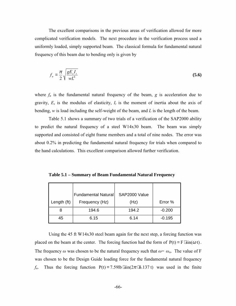
-66-
The excellent comparisons in the previous areas of verification allowed for more
complicated verification models. The next procedure in the verification process used a
uniformly loaded, simply supported beam. The classical formula for fundamental natural
frequency of this beam due to bending only is given by
42 wLIgEf ts
nπ= (5.6)
where fn is the fundamental natural frequency of the beam, g is acceleration due to
gravity, Es is the modulus of elasticity, It is the moment of inertia about the axis of
bending, w is load including the self-weight of the beam, and L is the length of the beam.
Table 5.1 shows a summary of two trials of a verification of the SAP2000 ability
to predict the natural frequency of a steel W14x30 beam. The beam was simply
supported and consisted of eight frame members and a total of nine nodes. The error was
about 0.2% in predicting the fundamental natural frequency for trials when compared to
the hand calculations. This excellent comparison allowed further verification.
Table 5.1 – Summary of Beam Fundamental Natural Frequency
Length (ft)
Fundamental Natural
Frequency (Hz)
SAP2000 Value
(Hz) Error %
8 194.6 194.2 -0.200
45 6.15 6.14 -0.195
Using the 45 ft W14x30 steel beam again for the next step, a forcing function was
placed on the beam at the center. The forcing function had the form of t)sin( F P(t) ω⋅= .
The frequency ω was chosen to be the natural frequency such that ω= ωn. The value of F
was chosen to be the Design Guide loading force for the fundamental natural frequency
fn. Thus the forcing function t)6.137sin(2 7.59lb P(t) ⋅⋅= π was used in the finite

-67-
element model. The 7.59 lb amplitude is equal to 65 lb*exp(-0.35(6.137)). Using the
hand calculation method provided by the Design Guide procedure, a peak acceleration ao
= 18.74% g is obtained. The finite element analysis yielded 18.66% g resulting in a
0.42% error. Once again this is a very excellent comparison.
The next step in verification was to add a uniform mass to the beam to see if the
finite element analysis will provide the same results as predicted by the hand calculations.
The mass was added to the beam by modifying the mass of the steel. For this step, there
was a 0.18% error in the fundamental natural frequency and a 0.13% error in the peak
accelerations. Another method of adding mass that was verified was to add lumped
masses at each node. This method produced only 0.09% error in the peak accelerations.
Either way, there were extremely accurate comparisons in the verification process as a
whole, which leads to the conclusion that the SAP2000 finite element program is not
flawed in its basic operation of dynamic analysis.
5.3 MESH REFINEMENT
The mesh refinement is a process that helps the finite element user determine the
best mesh to use in his testing. A mesh that is not optimized will either take too much
time to run if too many elements are used, or it will have poor accuracy if not enough
elements are used. Therefore a process is required to find the optimum number of
elements to use in the mesh.
The optimum number of elements for the mesh was determined by modeling a
beam with a concrete slab on the top and increasing the number of shell elements used for
the slab. The beam centroid formed a centerline to the slab looking in a plan-view of the
model. The best shell element to use is one with an aspect ratio of 1 (i.e., a square
element). A square element was used for the slab, starting with one row of shell elements
on each side of the beam. Then the shell elements were divided into four equal parts,
which made two rows of shell elements on each side of the beam. The process continued
until there were 16 shell elements on each side of the beam. Figure 5.6 shows a drawing
of the typical beam and slab finite element model with one shell element on each side of

-68-
the beam. Figure 5.7 shows a drawing of a model with two shell elements on each side of
the beam.
Figure 5.6 – One Shell Element on Each Side of Beam
Figure 5.7 –Two Shell Elements on Each Side of Beam
Each of the finite element models from one shell element on each side to sixteen
shell elements on each side was analyzed. A fundamental natural frequency, self-weight
deflection, and a point load deflection were calculated for each of the five meshes. Table
5.2 summarizes the data that were acquired from this analysis. After the data in Table 5.2

-69-
were generated, they were plotted to determine the optimum mesh. The three plots are
shown in Figures 5.8, 5.9, and 5.10. They give the same conclusion that mesh number
three, four elements per side, was best for use in this study. For a total slab width of 96
in., this would make each shell element 12 in. square. Thus for almost all models 12 in.
squares were used where applicable. The 12 in. square is also a convenient size for
modeling.
Table 5.2 – Data for mesh refinement
mesh number shells per side fn (Hz) self wt. defl (in.) pt. load defl. (in.)1 1 6.83 0.2534 0.02032 2 6.96 0.2494 0.01973 4 7.00 0.2484 0.01954 8 7.01 0.2481 0.01955 16 7.01 0.2480 0.0195
6.826.84
6.866.886.906.92
6.946.966.98
7.007.02
0 5 10 15 20
Shell Elements on Each Side of Centerline
Fund
amen
tal N
atur
al F
requ
ency
(Hz)
Figure 5.8 – Fundamental Natural Frequency Versus Number of Shell Elements per
Side

-70-
0.247
0.248
0.249
0.250
0.251
0.252
0.253
0.254
0 2 4 6 8 10 12 14 16 18
Shell Elements on Each Side of Centerline
Def
lect
ion
at M
idsp
an D
ue to
Sel
f W
eigh
t (in
.)
Figure 5.9 – Deflection Due to Self-Weight Versus Number of Shell Elements per
Side
0.01940.01950.01960.01970.01980.01990.02000.02010.02020.02030.0204
0 5 10 15 20
Shell Elements on Each Side of Centerline
Del
fect
ion
at M
idsp
an D
ue to
1ki
p Po
int L
oad
(in.)
Figure 5.10 – Deflection Due to Point Load Versus Number of Shell Elements per
Side

-71-
5.4 EFFECTIVE SLAB WIDTH OF FOOTBRIDGE
After determining an optimum number of shell elements to use for modeling the
slab, models with a concrete slab were analyzed and the results compared to the hand
calculations using the Design Guide procedure. The simplest model with a concrete slab
is that of a footbridge. Thus, hand calculations for a footbridge were performed and
compared with finite element data. There was a suspicion that the problem that caused
the finite element model to differ from hand calculations could lie within the area of the
effective slab width for vibration.
To attempt to make this comparison, the effective width be of the slab was
determined. This effective width is equal to the minimum of either the center-to-center
spacing of the members or 0.4 times the length of the supporting members. All shell
elements were square elements with a size of 12 in. x 12 in., which conveniently divided
the length of the beam into even sections. The value of the slab width s was substantially
larger than the be value. If the finite element analysis produced different numbers, then
that would indicate that the effective slab width that participated in vibration in the finite
element program would be different from what was assumed by the hand calculations.
Two sets of models were used. The first set of models used a beam length of 32 ft
and the second set used a 50 ft beam. The 32 ft beam was a W18x35 shape and the 50-ft
beam was a W33x118. The two data sets are summarized in the Tables 5.3 and 5.4. The
fundamental natural frequency and deflection due to self-weight were computed by the
finite element program and by use of the Design Guide procedures. A plot of the
SAP2000 values versus the theoretical hand calculated values for fn was analyzed for both
test cases. The only variable in each set of models was the beam spacing. The slab width
used in SAP2000 was the spacing, and the effective slab width be was used for the Design
Guide procedure. The beams were of sufficient length so that shear deformations could
be neglected.

-72-
Table 5.3 – 32 ft Beam Data
Model No.
s
(in.)
be
(in)
FE fn
(Hz)
Predicted fn
(Hz)
% difference
sw32-1 96 96 7.00 7.13 -1.84
sw32-2 144 144 5.89 6.03 -2.34
sw32-3 168 153.6 5.50 5.62 -2.14
sw32-4 192 153.6 5.18 5.27 -1.63
sw32-5 216 153.6 4.92 4.97 -1.09
sw32-6 240 153.6 4.69 4.73 -0.89
sw32-7 360 153.6 3.42 3.36 1.79
sw32-8 288 153.6 4.32 4.32 -0.12
Table 5.4 – 50 ft Beam Data
Model No.
s
(in.)
be
(in)
FE fn
(Hz)
Predicted fn
(Hz)
% difference
sw50-1 120 120 6.86 6.94 -1.17
sw50-2 168 168 6.08 6.19 -1.73
sw50-3 216 216 5.51 5.64 -2.25
sw50-4 240 240 5.28 5.42 -2.58
sw50-5 288 240 4.89 4.98 -1.89
sw50-6 360 240 4.43 4.48 -1.18
sw50-7 408 240 4.18 4.22 -0.92
sw50-8 480 240 3.88 3.91 -0.84
Figure 5.11 shows a typical cross-section of the footbridge finite element model (FEM)
created in SAP2000. The data gathered from these experiments showed that there was
little difference between the predicted fundamental natural frequencies and the finite
element natural frequencies. Figures 5.12 and 5.13 contain data plots of fundamental
natural frequencies for finite element analyses versus the predicted values for each
system of beams. The solid line is the one-to-one slope on which every point should
theoretically lie.

-73-
Figure 5.11 – Typical Cross-Section of Footbridge and FEM
32 ft beam
3.003.504.004.505.005.506.006.507.007.508.00
3.00 4.00 5.00 6.00 7.00 8.00
Predicted fn (Hz)
FE f
n (H
z)
Figure 5.12 – Difference Plots for 32 ft Beam System
a) b)

-74-
50 ft Beam
3.003.504.004.505.005.506.006.507.007.508.00
3.00 4.00 5.00 6.00 7.00 8.00
Predicted fn (Hz)
FE f n
(Hz)
Figure 5.13 – Difference Plots for 50 ft Beam System
It is obvious that the problem does not lie within this area of the study. These
plots show very little error between the two methods of analysis. Because of this, larger
systems with more complex framing (several beams) can start to be compared to each
other. The peak acceleration values matched just as well. They are included in the
results in the following section on multiple beam systems.
5.5 MULTIPLE BEAM SYSTEMS
After determining that the Design Guide effective slab width for a one-beam
system was correct, larger systems that included multiple beams were studied. The
systems started off as a one-beam footbridge and were enlarged to a wide bay-like
footbridge with many beams. All beams were simply supported.
The sinusoidal forcing function prescribed by the Design Guide was applied at the
center of the finite element floor. The peak acceleration obtained by the analysis was
compared to the value obtained from hand calculations. The assumption of the hand
calculation method is that after the system reaches a certain width, it changes from a
footbridge to a bay. For the assumption of a footbridge, the whole mass is used in the

-75-
calculation. If the system is too wide to be considered a footbridge, the mass beyond the
effective panel width Bj is not assumed to participate in the vibration due to damping over
an extended area in the system. These sources of damping are due to frictional damping
and energy dispersion. Equation 5.7 is used to calculate Bj.
jjsjj LDDCB 4/1)/(= (5.7)
where Ds = transformed slab moment of inertia per unit width, Dj = effective moment of
inertia of tee-beam per unit width, and Cj = 2 for most joists or beams and 1 for joists or
beams parallel to an interior edge. If the edge joist or beam is more than 50% stiffer than
the interior beams or joists, Cj is taken as 2, even though it is an edge member. Lj is the
length of the joist or beam. The value of Bj has a maximum of 2/3 of the floor-width in
direction of the beams.
When this value of Bj is calculated, it is used in determining the effective mass of
the whole panel that participates in vibration. Since this value is limited to a maximum
of 2/3 the beam-length in this case, when the length perpendicular to the beams exceeds a
certain value, Bj no longer increases though the whole mass of the system does. This
increases the peak acceleration obtained from hand calculations compared to that
obtained from a finite element model. The finite element model cannot take into account
frictional damping and energy dispersion. Thus, over a long enough period of time the
whole width of the system actively participates in the vibration as it assumes the first
modal shape. This is only natural as the frequency at which the bay is being driven is the
frequency of the first mode shape.
An animated video created by the finite element program illustrates the
displacement of the floor during the excitation. The largest motion occours at the source
of the input and the other displacements ripple out in waves similar to those found in a
pond after a rock is tossed. Unlike the rock-in-the-pond analogy, the forcing function is
not removed. For this reason, after enough time is elapsed, the displacement trace of the
whole bay is almost exactly like the first mode shape. The first mode shape has the same
basic shape for each bay that was investigated. This mode shape is illustrated in Figure
5.14.

-76-
Figure 5.14 – Typical Mode Shape for the Fundamental Natural Frequency
In Figure 5.14, the beams are parallel to the Y-axis (short direction) and the
supports are along the edges in the direction parallel to the X-axis (long direction). The
only modal participation at the supported ends was from rotation and not displacement.
Plots of acceleration versus number of beams were created. These systems had
evenly spaced beams. The plots show that the acceleration calculated by the AISC
Design Guide criterion levels off after the system becomes greater than the effective
panel width, Bj. On the other hand, the finite element models are asymptotic to zero.
This shows that there is no limit to the width of the participating mass in the bay when
using finite element analysis. These plots are shown in Figures 5.15 and 5.16. The plot
in Figure 5.15 is for data from a system with 50 ft beams spaced at 14 ft on-center. The
system had a fundamental natural frequency of 6 Hz. The plot in Figure 5.16 is from a
system with 25 ft beams spaced at 10 ft on-center. The fundamental natural of this
system was 10 Hz. Damping for these two systems was 3% of critical damping.
Both of the following figures show the relation between values from the Design
Guide calculations and two types of finite element models. The first type of finite
element model was created using SAP2000, and it only allowed one-way bending in the
system. The second type of finite element model was also created using SAP2000 and all
degrees of freedom were considered in the analysis.

-77-
00.05
0.10.15
0.20.25
0.30.35
0.40.45
0.5
0 2 4 6 8 10
Number of Beams
Acc
eler
atio
n (a
/g %
)Design GuideSAP 1-waySAP all DOF
Figure 5.15 - Acceleration for System Versus Number of 50 ft Beams
0
0.05
0.1
0.15
0.2
0.25
0.3
0 2 4 6 8
Number of Beams
Acc
eler
atio
n (a
/g %
)
Design GuideSAP 1-waySAP all DOF
Figure 5.16 – Acceleration for System Versus Number of 25 ft Beams
Every finite element analysis matched very well with the hand calculations for a
footbridge model (for one beam) when bending in only one direction was considered.
However, the finite element analysis results were very different from the hand calculation
results when the FE model was not restrained in a simple bending mode. It is also seen
in the plots that the peak acceleration values match for the system with one beam, where
the system is considered a footbridge. However, for larger systems the Bj value

-78-
approaches the limiting value of 2/3 of the length of the floor for the hand calculations.
SAP2000 cannot be used if the effects due to energy dispersion and frictional damping
(which increases with panel area) are to be considered. Thus, the accumulation of these
effects causes acceleration values from SAP2000 to become asymptotic to zero as the
number of beams increases.
5.6 MULTIPLE BAY SYSTEM
The discrepancy is obviously between the assumptions of the effective panel
width calculation and not being able to account for these assumptions in SAP2000. This
problem can carry over to systems having multiple bays. So it was important to solve the
problem on the simplified systems first. The attempt to modify finite element models to
match the results of the AISC Design Guide criterion was also made. Many different
techniques were attempted in order to reach this goal.
The reason for trying to match the AISC criterion by the finite element models
was to shed light on the source of the discrepancy. Placing columns for rotational
restraints, omitting portions of mass within the bay, plotting static deflection, breaking
down the acceleration components by the modal participation, and applying alternate
forcing functions were some of the techniques used to obtain matching accelerations. All
of these were performed before the source of the difference in the FE models and
hand calculations was realized. That source of the difference is that SAP2000 did not
include frictional damping and energy dispersion like the hand calculations account for.
For this reason, the methods are described with their basic results and why they did not
work. Excessive detail is not provided because they are all tangential to the direction of
finding a solution.
Placing columns as rotational restraints changes the frequency of the system
depending on the column stiffness. This approach does not help because it changes the
frequencies as compared to the hand calculations, which do not consider the stiffness of
the columns. This method is not recommended because it does not use the same
modeling assumptions as the hand calculations.

-79-
Portions of mass were omitted in the bay beyond the effective panel width. This
drastically increased the natural frequency of the system. This increase in natural
frequency of the system makes the results even worse because previously it was possible
to match peak accelerations.
Static deflection plots were made to see what was happening in the SAP2000
model. A static point load was placed in the middle of the bay, and the resulting
deflected shape was plotted. The distances to the inflection points were measured to see
if there was some relation between this and the effective panel width. This was done
with the expectation that a new effective panel width equation could be determined from
FE models. However, this was done before realizing that SAP2000 did not include
frictional damping that increases with panel area. Thus, none of these plots were of any
use since the source of error most likely lies within the FE models instead of the hand
calculations.
To obtain the modal contributions, the acceleration trace was analyzed to obtain
the peak acceleration. The components of the acceleration trace were then broken down
according to each mode and analyzed to determine the relative contribution of each mode
shape. The thought behind this was that participation of higher modes in SAP2000 could
have been causing some discrepancy between the hand calculations and the FE models.
Table 5.5 shows an example of a system that had a peak acceleration of 0.2274% g. The
table shows that almost all of the contribution is from the first mode and the error was not
because of this.
Table 5.5 - Modal Contributions
Mode
Freq.
(Hz)
Acceleration
(% g)
Mode
Freq.
(Hz)
Acceleration
(% g)
1 3.10 -0.1952 6 23.37 0.0000
2 11.72 0.0000 7 26.95 -0.0005
3 12.24 -0.0205 8 27.70 0.0000
4 17.06 0.0000 9 33.11 0.0000
5 23.81 -0.0111 10 35.21 0.0000

-80-
Forcing functions at different frequencies were used in order to attempt a match
of the FE model results with the hand calculations. However, the forcing functions that
produce the maximum peak acceleration are those which have the same frequency as that
of the first natural frequency of the floor. All other frequencies produce a smaller peak
acceleration value. This was not desired in this case, since the peak accelerations from
the FE models were already too small.
None of these methods prevailed in bridging the gap between peak accelerations
obtained from finite element models and those derived from hand calculations.
5.7 CONCLUSIONS AND SUMMARY OF RESULTS
All of the FE results matched the Design Guide procedure results well until the
system width exceeded the effective panel width calculated from the design guide
calculations. The error definitely lies within this area. The problem is that SAP2000
cannot directly account for frictional damping in systems, nor can it account for energy
dispersion. The only damping it can consider is viscous modal damping. The effective
panel width equation accounts for effects of energy dispersion and frictional damping,
which increases with increased panel size. Further research is required in this area to find
an appropriate way to account for these effects by using FE models.

-81-
CHAPTER VI
CONCLUSIONS AND RECOMMENDATIONS
6.1 INTRODUCTION
This chapter presents the final conclusions derived from the four main areas of
this study.
The first area of research dealt compared finite element models with real
structural systems. These structural systems were simple systems. This provided an
opportunity to explore modeling techniques of a cantilever staircase and to see how well
a heel-drop trace could be simulated in the model. The other structural system was the
Virginia Tech Laboratory Floor. This simple system modeling allowed experimentation
with retrofits to reduce vibration.
The second area of research also used the Virginia Tech Laboratory Floor. The
floor was used for various experiments. All of these experiments were focused on
comparing finite element models with test data. The first experiment was done to
measure damping. The second experiment was done to compare mode shapes. The third
experiment was done to compare peak accelerations with a known sinusoidal forcing
function.
The third area of research was done to find an inexpensive method of field-testing
for a floor system. This method of testing would determine the acceptability of the floor
system with a quick evaluation and without use of a finite element model.
The fourth area of research was an analytical pursuit of the source of difference
between the accelerations determined by the procedure in the AISC Design Guide and the
accelerations produced by a finite element model.
Also found in this chapter are areas of future research.

-82-
6.2 GENERAL CONCLUSIONS
6.2.1 Research Area One – The Staircase and Retrofits
The staircase experiment did not yield very good results. The actual staircase had
a natural frequency of 7.5 Hz and the finite element model yielded a frequency of 11.0
Hz.
The experiment with the retrofits on the Virginia Tech Lab floor showed that
different locations on the floor can experience different annoying frequencies. Those
frequencies that are most annoying are based on how close an occupant is to an anti-node
for a certain mode. The experiment also shows how a second-mode frequency could be
more disturbing than the fundamental natural frequency to people on portions of the floor
where the anti-nodes for this second mode occur. Another factor in determining the most
annoying frequency for a particular system is the excitation frequency.
Another discovery from this area of research was that a retrofit should be placed
at the anti-node of the most annoying frequency of the floor instead of necessarily at the
center. Placement of a retrofit at the center is satisfactory when the most annoying
frequency is the fundamental natural frequency. This is because the anti-node for that
mode shape is usually located there. However, if complaints from occupants arise from
areas that are affected more by higher modes, then placing the retrofit at the center of the
bay will not be the most effective method of vibration reduction.
The best type of retrofit used posts and a spreader-beam assembly. The second
best retrofit used only the post at a point location, and supported the floor on the
underside of the deck. However, the retrofit with the spreader-beam provided a larger
contact area. The spreader-beam supported the floor on the bottom of the top chord of
the joists. This caused the load transfer to go from a larger area of the slab to the joists
and then to the post. This could possibly help reduce rotation of other modes, which
would reduce their participation in vibration depending on how much rotational restraint
is provided by the spreader-beam assembly.

-83-
6.2.2 Research Area Two – Virginia Tech Lab Floor Experiments
Damping measurement on the Virginia Tech Lab Floor did not match the assumed
value. The value of damping obtained (2.04% of critical) was about twice as much as
what was expected for an empty floor. This caused the values of peak acceleration to not
match the finite element model. If the damping were in the range of 1.32% to 1.61% of
critical damping, then the peak acceleration values would have matched. The
Experimental Modal Analysis (EMA) provided a mode shape plot with an excellent
match to the finite element data. This research shows that the mode shapes that really
exist in a floor can be predicted well with a finite element model.
6.3.3 Research Area Three – Field Evaluation
The results from this area of research could not be used to establish a practical
method for determining the acceptability of a floor by only using a hand-held analyzer,
an accelerometer, and a series of walking tests. Also, measurements at more than one
location on a bay are needed, depending on where the occupants are located.
Several data points on each bay should be read to determine the frequencies that
contribute to annoying vibrations. The FFT spectrum will provide the frequencies that
contribute the most to vibration in each area of the floor. This data can then be compared
to the results of a finite element analysis to determine which mode shape contributes most
to the vibration. After the problem mode shape is determined, a retrofit can be placed in
a location that would best eliminate or limit participation of the problem mode. The best
location for a retrofit is at an anti-node.
The use of a finite element model is required for a detailed analysis instead of
hand calculations if the first mode shape is not the mode shape that contributes to the
most annoying vibration. The finite element analysis is the only method used in this
study that will predict multiple mode shapes and their corresponding frequencies.
6.3.4 Research Area Four – Missing Link Between AISC and FE Methods
All of the results matched well until the system width exceeded the effective
panel width calculated from the Design Guide criteria. The error definitely lies within
this area. The problem is that SAP2000 cannot directly account for frictional damping in

-84-
systems, nor can it account for energy dispersion. The only damping it can consider is
viscous modal damping. The effective panel width equation accounts for effects of
energy dispersion and frictional damping, which increases with increased panel size.
Further research is required in this area to find an appropriate way to account for these
effects by using FE models. Due to this error, larger floor systems modeled will have
matching frequencies, but the peak accelerations will not match. Although the location
of the problem was established, a solution could not be determined from this research.
6.3 AREAS OF FUTURE RESEARCH
6.3.1 Modeling considerations
There are many areas possible for future research in the field of floor vibrations.
The first part of this study (in Chapter II) left an opening in the area of the finite element
modeling. Instead of assuming rigid supports for the retrofit posts, they could have been
modeled as springs with appropriate stiffnesses. This closer investigation would provide
more accurate results in predicting the effectiveness of retrofits in floor systems.
A finite element model for predicting the heel-drop spectrum and natural
frequency of a cantilever staircase was not accomplished. Further research in this area
could be explored. This would be especially useful if the natural frequency of the
staircase was such that it excited the natural frequency of the floor system to which it is
attached. The reason for this is that annoying vibration on a floor system could come
from the staircase, which is not considered in hand calculations.
6.3.2 Other areas of research
Further research in the area of floor vibrations is needed where the AISC Design
Guide does not provide methods to analyze certain floors by simple hand calculations.
Such floors cannot use these hand calculations due to inherent complexities. A lot of
research is needed in the computer modeling aspect of floor vibrations.

-85-
List of References
Allen, D. E., and Murray, T. M. (1993). �Design Criterion for Vibrations Due to Walking.� AISC Engineering Journal, 4th qtr., 117-129.
Band, B. S. Jr. (1996). �Vibration Characteristics of Joist and Joist-Girder Members.�
M.S. Thesis, Virginia Polytechnic Institute and State University, Blacksburg, Virginia.
Beavers, T. A. (1998). �Fundamental Natural Frequency of Steel Joist Supported Floors�
M.S. Thesis, Virginia Polytechnic Institute and State University, Blacksburg, Virginia.
Gibbings, D. R., Easterling, W. S., and Murray, T. M. (1993). �Analysis of Composite
Joists.� Report No. CE/VPI 93/12. Virginia Polytechnic Institute and State University, Blacksburg, Virginia.
Hanagan, L. M. (1994). �Active Control of Floor Vibrations.� Ph. D. Dissertation,
Virginia Polytechnic Institute and State University, Blacksburg, Virginia. Lenzen, Kenneth H. (1966). �Vibration of Steel Joist Concrete Slab Floors.�
Engineering Journal, American Institute of Steel Construction, 2(3), pp. 133-136. Murray, T. M. (1975). �Design to Prevent Floor Vibrations.� Engineering Journal, AISC,
12(3), 82-87. Murray, T. M. (1981). �Acceptability Criteria for Occupant-Induced Floor Vibrations.�
Engineering Journal, AISC, 18(2), 62-69. Murray, T.M. (1991) �Building Floor Vibrations� Engineering Journal, AISC, 28(3), pp.
102-109. Murray, T. M., Allen, D.E and Ungar, E. E. (1997). AISC Steel Design Guide Series 11:
Floor Vibrations Due to Human Activity. American Institute of Steel Construction, Chicago.
Reiher, H. and Meister, F. J. (1931). �The Effect of Vibration on People� (in German).
Forchung auf dem Gebetite des Ingenieurwesens, 2(2), p. 381. (Translation: Report no. F-TS-616-Re H.Q. Air Material Command, Wright Field, Ohio, 1949).
Rottmann, C. E. (1996). �Use of Tuned-Mass Dampers to Control Annoying Floor
Vibrations.� M.S. Thesis, Virginia Polytechnic Institute and State University, Blacksburg, Virginia.
Shamblin, C. L. (1989). �Floor System Response to Heel-Drop Impact.� M.S.Thesis,
Virginia Polytechnic Institute and State University, Blacksburg, Virginia.

-86-
Sladki, M. J. (1999). �Prediction of Floor Vibration Response Using the Finite
Element Method.� M.S. Thesis, Virginia Polytechnic Institute and State University, Blacksburg, Virginia. Treadgold, T. (1828). Elementary Principles of Carpentry, 2nd Ed., Publisher unknown.

-A-
APPENDIX A
CANITLEVER STAIRCASE PLANS
The plans of the cantilever staircase include only structural members that are
essential to strength. The railing components are not shown here, as they are not
essential to the modeling process (with the exception of addition of weight and mass).
The supports are on the left side of the staircase and were modeled as fixed supports.
Figure A.1 – Plan View of Staircase

-B-
Figure A.2 – Elevation View of Staircase

-C-
APPENDIX B
DESIGN GUIDE CALCULATIONS FOR LAB FLOOR
VIBRATION ANALYSIS:
Activity: Walking Occupancy Category: Office or Residence Evaluation Criterion: Walking, AISC Design Guide, Chapter 4 Reference: Murray, T.M., Allen, D.E. and Ungar, E.E,
"Floor Vibrations Due To Human Activity", Design Guide, June 1997
Constant Force, Po = 65 lb Modal Damping Ratio, ß = 0.03 Acceleration Limit, ao/g x 100% = 0.50 % Joist bottom chords are not extended Girders are not continuous at columns Section w, plf Itr,in4 f, Hz. Beam joist 116.9 1960.4 8.49 Left Girder jg 896.3 2988.1 8.15 Right Girder jg 896.3 2988.1 8.15 Bay (Using smaller girder frequency) 5.88 Evaluation: Combined mode ap/g= 0.79 % > 0.50 % The system DOES NOT SATISFY THE CRITERION. LOADING DATA: 3.1c psf Deck = 33.5 psf Dead loads = 0.0 psf Collateral loads = 0.0 psf Live loads = 0.001 psf Actual beam and girder weights Tributary width for girder = 44.00/2 = 22.00 ft.

-D-
CONCRETE/SLAB DATA: Concrete dc= 3.00 in. fc'= 3.5 Ksi wt= 145 pcf Ec= 3267 Ksi Modular ratio, n= Es/(1.35 Ec) = 6.58 Deck height: 0.625 in. Effective concrete thickness in deck: 0.3125 in. SUPPORTED MEMBER CALCULATIONS: Built-up member: joist (16.4 plf) A= 4.824 in.2 Ichords= 1412 in.4 yc= 15.86 in. Spacing: S = 36 in. Span: Lj = 44.00 ft. Uniform load: wj = (33.5 + 0.0 + 0.0 + 0.001) x 36.00/12 + 16.4 = 116.9 plf Moment of inertia:
Effective concrete width = min(0.4 Lj, S) = 36.000 in. Effective concrete depth = 2.375 in. Transformed concrete width = 5.475 in. Transformed concrete area = 13.003 in.2 Distance to neutral axis (Above joist c.g.) = 13.935 in. Tr. moment of inertia using actual chords Icomp = 2517.0 in.4
6 < Lj/D = 14.67 < 24 (OK)
Cr = 0.90[1-exp(-0.28(L/D))]2.8 = 0.8627
1592.018627.0111 =−=−=
rCγ
4in. 4.1960
0.25171
14121592.0
11
1 =+
=+
=
compchords
eff
II
Iγ
in173.04.1960384172800.449.1165
3845
δ44
=××
×××=×
=seffj
jjj EIE
Lw
Frequency = 0.18 x [g / δj]0.5 = 0.18 x [386 / 0.173]0.5 = 8.49 Hz.

-E-
Cj = 1.0 Floor Width = 30.00 ft. Ds = (12 de
3)/(12 n) = (12 x 2.68753)/(12 x 6.58) = 2.95 in4/ft.
Dj = Ieff/S = 1960.4/3.00
= 653.47 in4/ft. Bj = min[Cj (Ds/Db)0.25 Lj= 11.40 ft.; 2/3 x 30.00 ft.= 20.00 ft.] = 11.40 ft. Continuity Factor=1.0 since max. adj. Lj=0.0 ft < 0.7 Lj=30.80 ft. Wj = wBjLj (w is weight supported per unit area) Wj = 1.0 x (0.117/3.00) x 11.40 x 44.00 = 19.6 Kips GIRDER CALCULATIONS: Built-up member: jg (38.9 plf) A= 11.44 in.2 Ix= 3270 in.4 yc= 18.00 in. Tributary width = 22.00 ft. Span: Lg = 30.00 ft. Equivalent uniform load: wg = 22.00 x (116.9/3.00) + 38.9
= 896.3 plf Moment of inertia: Min[0.2 Lg, Lg/2] = 72.000 " (10.950" transformed)
Effective concrete width = 72.000 in. and 36.000 in. Transformed concrete width = 10.950 in. and 5.475 in. Transformed concrete area = 26.006 in.2 and 3.422 in.2 Joist Seat Depth = 5.00 in. Distance to neutral axis = 13.907 in. (Above girder c.g.) Transformed moment of inertia Icomp = 8224 in.4

-F-
6 < Lj/D = 10.00 < 24 (OK)
Cr = 0.90[1-exp(-0.28(L/D))]2.8 = 0.7550
3245.017550.0111 =−=−=
rCγ
4in. 4528
82241
32703245.0
11
1 =+
=+
=
compchords
eff
II
Iγ
Imod = CrIChords Ig = Imod + (Ieff - Imod) = (0.755)(3270) + (1/4)[4528 � 0.755(3270)] = 2988.13 in.4
in.189.013.2988384172800.303.8965
3845
δ44
=××
×××=×
=sgs
ggg EIE
Lw
Frequency = 0.18 x [g / δb]0.5 = 0.18 x [386 / 0.189]0.5 = 8.15 Hz. Cg = 1.6 Floor Length = 44.00 ft. Db = Itr/S = 1960.4/3.00
= 653.47 in4/ft. Dg = Itr/Avg. Lb = 2988.1/22.00
= 135.82 in4/ft. Bg = min[Cg (Db/Dg)0.25 Lg= 71.09 ft.; 2/3 x 44.00 ft.= 29.33 ft.]
= 29.33 ft. Continuity Factor = 1.0 since Not Continuous Wg = wBgLg (w is weight supported per unit area) Wg = 1.0 x (0.896/22.00) x 29.33 x 30.00
= 35.9 Kips

-G-
COMBINED MODE CALCULATIONS: Using girder with smaller frequency: δb = 0.173 in. δg = 0.189 in. System frequency, fn= 0.18 [386/( δb+ δg)]=5.88 Hz Wb= 34.3 Kips Wg = 35.9 kips
ggb
bb
gb
b wwδδ
δδδ
δ+
++
=cw
Wc = [(0.173/0.362) x 19.6] + [(0.189/0.362) x 35.9] = 28110 lbs ß = modal damping ratio = 0.03 (ap/g) = [Po e (-0.35 fn)]/(ß Wc) = [65 e (-0.35 x 5.88)]/(0.03 x 28110) = 0.99 % > 0.50 % - DOES NOT SATISFY CRITERION
Since fn= 5.88 Hz ≤ 9 Hz - Stiffness criterion does not need to be checked.

-H-
APPENDIX C
FRF SPECTRA PLOTS
These FRF Spectra Plots are taken from the data readings on the Virginia Tech
laboratory floor during the retrofit tests.
0
0.00005
0.0001
0.00015
0.0002
0.00025
0.0003
0.00035
0.0004
0 5 10 15 20 25Frequency (Hz)
Acc
eler
atio
n (g
)
Figure C.1 – FRF Spectrum from Ambient Excitation for TCN 1
0
0.002
0.004
0.006
0.008
0.01
0.012
0 5 10 15 20 25Frequency (Hz)
Acc
eler
atio
n (g
)
Figure C.2 – FRF Spectrum for Heel Drop Excitation for TCN 1

-I-
0
0.001
0.002
0.003
0.004
0.005
0.006
0.007
0 5 10 15 20 25Frequency (Hz)
Acc
eler
atio
n (g
)
Figure C.3 – FRF Spectrum for Walking Parallel Excitation for TCN 1
0
0.001
0.002
0.003
0.004
0.005
0.006
0.007
0.008
0.009
0 5 10 15 20 25Frequency (Hz)
Acc
eler
atio
n (g
)
Figure C.4 – FRF Spectrum for Walking Perpendicular Excitation for TCN 1

-J-
0.000
0.001
0.002
0.003
0.004
0.005
0.006
0.007
0.008
0.009
0.010
0 5 10 15 20 25Frequency (Hz)
Acc
eler
atio
n (g
)
Figure C.5 – FRF Spectrum for Bouncing Excitation for TCN 1
0.000000.000020.000040.000060.000080.000100.000120.000140.000160.000180.00020
0 5 10 15 20 25Frequency (Hz)
Acc
eler
atio
n (g
)
Figure C.6 – FRF Spectrum for Ambient Excitation for TCN 2
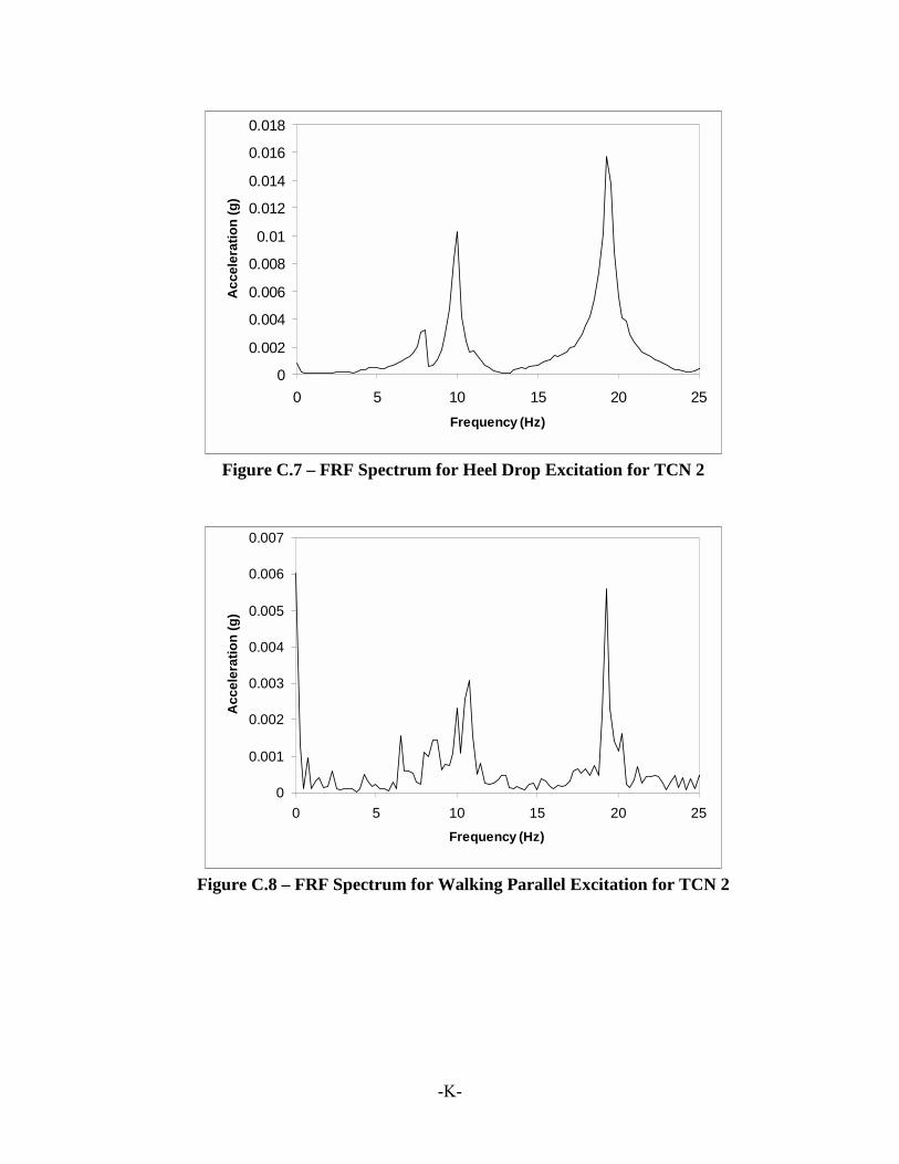
-K-
0
0.002
0.004
0.006
0.008
0.01
0.012
0.014
0.016
0.018
0 5 10 15 20 25Frequency (Hz)
Acc
eler
atio
n (g
)
Figure C.7 – FRF Spectrum for Heel Drop Excitation for TCN 2
0
0.001
0.002
0.003
0.004
0.005
0.006
0.007
0 5 10 15 20 25Frequency (Hz)
Acc
eler
atio
n (g
)
Figure C.8 – FRF Spectrum for Walking Parallel Excitation for TCN 2

-L-
0
0.0005
0.001
0.0015
0.002
0.0025
0.003
0.0035
0 5 10 15 20 25Frequency (Hz)
Acc
eler
atio
n (g
)
Figure C.9 – FRF Spectrum for Walking Perpendicular Excitation for TCN 2
0
0.001
0.002
0.003
0.004
0.005
0.006
0.007
0.008
0 5 10 15 20 25Frequency (Hz)
Acc
eler
atio
n (g
)
Figure C.10 – FRF Spectrum for Bouncing Excitation for TCN 2

-M-
0
0.000005
0.00001
0.000015
0.00002
0.000025
0.00003
0.000035
0.00004
0.000045
0 5 10 15 20 25Frequency (Hz)
Acc
eler
atio
n (g
)
Figure C.11 – FRF Spectrum for Ambient Excitation for TCN 3
0
0.005
0.01
0.015
0.02
0.025
0.03
0 5 10 15 20 25Frequency (Hz)
Acc
eler
atio
n (g
)
Figure C.12 – FRF Spectrum for Heel Drop Excitation for TCN 3

-N-
0
0.001
0.002
0.003
0.004
0.005
0.006
0.007
0.008
0 5 10 15 20 25Frequency (Hz)
Acc
eler
atio
n (g
)
Figure C.13 – FRF Spectrum for Walking Parallel Excitation for TCN 3
0
0.001
0.002
0.003
0.004
0.005
0.006
0.007
0 5 10 15 20 25Frequency (Hz)
Acc
eler
atio
n (g
)
Figure C.14 – FRF Spectrum for Walking Perpendicular Excitation for TCN 3

-O-
0
0.0010.002
0.003
0.0040.005
0.006
0.007
0.0080.009
0.01
0 5 10 15 20 25Frequency (Hz)
Acc
eler
atio
n (g
)
Figure C.15 – FRF Spectrum for Bouncing Excitation for TCN 3
0.00000
0.00001
0.00002
0.00003
0.00004
0.00005
0.00006
0.00007
0.00008
0.00009
0.00010
0 5 10 15 20 25Frequency (Hz)
Acc
eler
atio
n (g
)
Figure C.16 – FRF Spectrum for Ambient Excitation for TCN 4

-P-
0
0.005
0.01
0.015
0.02
0.025
0 5 10 15 20 25Frequency (Hz)
Acc
eler
atio
n (g
)
Figure C.17 – FRF Spectrum for Heel Drop Excitation for TCN 4
0
0.001
0.002
0.003
0.004
0.005
0.006
0 5 10 15 20 25Frequency (Hz)
Acc
eler
atio
n (g
)
Figure C.18 – FRF Spectrum for Walking Parallel Excitation for TCN 4

-Q-
0
0.001
0.002
0.003
0.004
0.005
0.006
0 5 10 15 20 25Frequency (Hz)
Acc
eler
atio
n (g
)
Figure C.19 – FRF Spectrum for Walking Perpendicular Excitation for TCN 4
0
0.001
0.002
0.003
0.004
0.005
0.006
0.007
0 5 10 15 20 25Frequency (Hz)
Acc
eler
atio
n (g
)
Figure C.20 – FRF Spectrum for Bouncing Excitation for TCN 4

-R-
0
0.00002
0.00004
0.00006
0.000080.0001
0.00012
0.00014
0.00016
0.00018
0.0002
0 5 10 15 20 25Frequency (Hz)
Acc
eler
atio
n (g
)
Figure C.21 – FRF Spectrum for Ambient Excitation for TCN 5
0
0.002
0.004
0.006
0.0080.01
0.012
0.014
0.016
0.018
0.02
0 5 10 15 20 25Frequency (Hz)
Acc
eler
atio
n (g
)
Figure C.22 – FRF Spectrum for Heel Drop Excitation for TCN 5

-S-
0
0.0005
0.001
0.0015
0.002
0.0025
0.003
0.0035
0 5 10 15 20 25Frequency (Hz)
Acc
eler
atio
n (g
)
Figure C.23 – FRF Spectrum for Walking Parallel Excitation for TCN 5
0
0.001
0.002
0.003
0.004
0.005
0.006
0.007
0.008
0.009
0 5 10 15 20 25Frequency (Hz)
Acc
eler
atio
n (g
)
Figure C.24 – FRF Spectrum for Walking Perpendicular Excitation for TCN 5

-T-
0
0.0005
0.001
0.0015
0.002
0.0025
0.003
0.0035
0 5 10 15 20 25Frequency (Hz)
Acc
eler
atio
n (g
)
Figure C.25 – FRF Spectrum for Bouncing Excitation for TCN 5
0
0.0001
0.0002
0.0003
0.0004
0.0005
0.0006
0 5 10 15 20 25Frequency (Hz)
Acc
eler
atio
n (g
)
Figure C.26 – FRF Spectrum for Ambient Excitation for TCN 6

-U-
0
0.005
0.01
0.015
0.02
0.025
0 5 10 15 20 25Frequency (Hz)
Acc
eler
atio
n (g
)
Figure C.27 – FRF Spectrum for Heel Drop Excitation for TCN 6
0
0.001
0.002
0.003
0.004
0.005
0.006
0.007
0.008
0.009
0.01
0 5 10 15 20 25Frequency (Hz)
Acc
eler
atio
n (g
)
Figure C.28 – FRF Spectrum for Walking Parallel Excitation for TCN 6
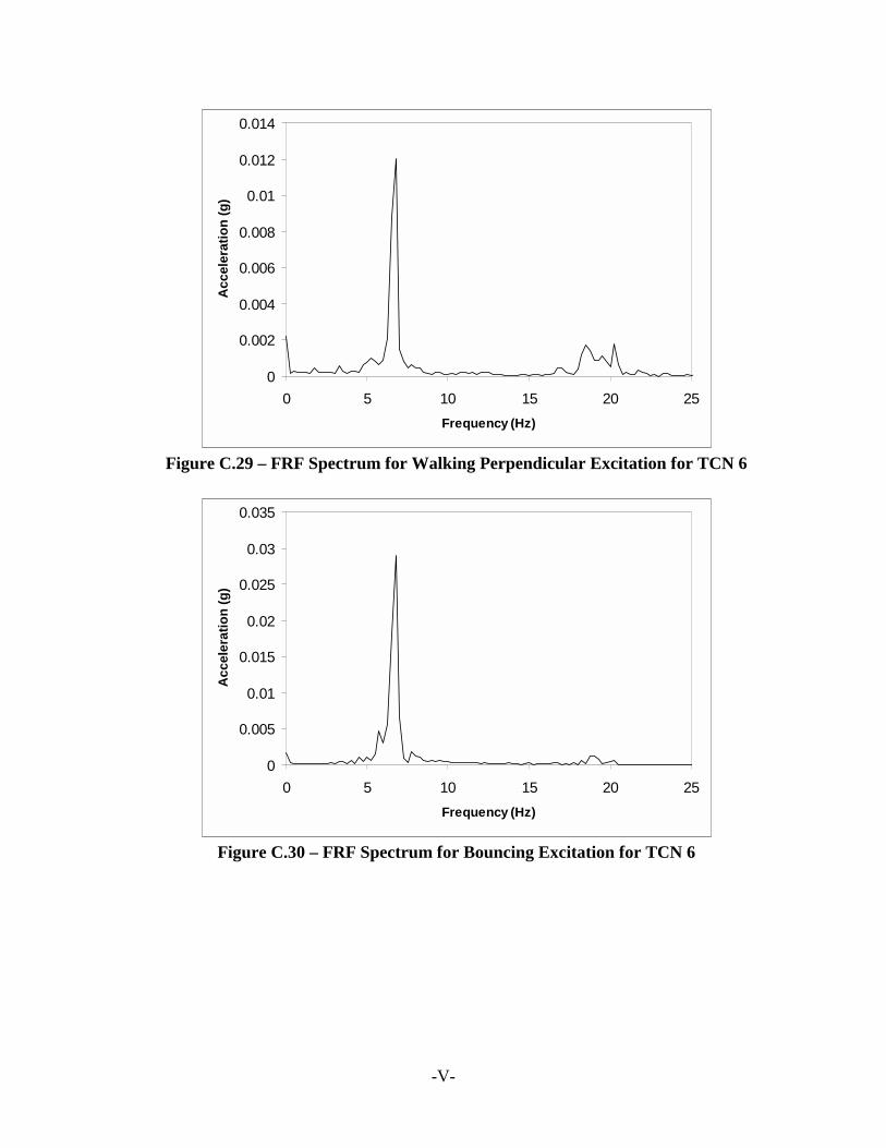
-V-
0
0.002
0.004
0.006
0.008
0.01
0.012
0.014
0 5 10 15 20 25Frequency (Hz)
Acc
eler
atio
n (g
)
Figure C.29 – FRF Spectrum for Walking Perpendicular Excitation for TCN 6
0
0.005
0.01
0.015
0.02
0.025
0.03
0.035
0 5 10 15 20 25Frequency (Hz)
Acc
eler
atio
n (g
)
Figure C.30 – FRF Spectrum for Bouncing Excitation for TCN 6

-W-
0
0.00002
0.00004
0.00006
0.00008
0.0001
0.00012
0.00014
0 5 10 15 20 25Frequency (Hz)
Acc
eler
atio
n (g
)
Figure C.31 – FRF Spectrum for Ambient Excitation for TCN 7
0
0.002
0.004
0.006
0.008
0.01
0.012
0.014
0.016
0.018
0.02
0 5 10 15 20 25Frequency (Hz)
Acc
eler
atio
n (g
)
Figure C.32 – FRF Spectrum for Heel Drop Excitation for TCN 7

-X-
0
0.001
0.002
0.003
0.004
0.005
0.006
0.007
0 5 10 15 20 25Frequency (Hz)
Acc
eler
atio
n (g
)
Figure C.33 – FRF Spectrum for Walking Parallel Excitation for TCN 7
0
0.001
0.002
0.003
0.004
0.005
0.006
0 5 10 15 20 25Frequency (Hz)
Acc
eler
atio
n (g
)
Figure C.34 – FRF Spectrum for Walking Perpendicular Excitation for TCN 7

-Y-
0
0.0005
0.001
0.0015
0.002
0.0025
0.003
0.0035
0.004
0 5 10 15 20 25Frequency (Hz)
Acc
eler
atio
n (g
)
Figure C.35 – FRF Spectrum for Bouncing Excitation for TCN 7
0
0.00005
0.0001
0.00015
0.0002
0.00025
0.0003
0.00035
0.0004
0.00045
0.0005
0 5 10 15 20 25Frequency (Hz)
Acc
eler
atio
n (g
)
Figure C.36 – FRF Spectrum for Ambient Excitation for TCN 8

-Z-
0
0.002
0.004
0.006
0.008
0.01
0.012
0.014
0.016
0.018
0 5 10 15 20 25Frequency (Hz)
Acc
eler
atio
n (g
)
Figure C.37 – FRF Spectrum for Heel Drop Excitation for TCN 8
0
0.002
0.004
0.006
0.008
0.01
0.012
0.014
0.016
0 5 10 15 20 25Frequency (Hz)
Acc
eler
atio
n (g
)
Figure C.38 – FRF Spectrum for Walking Parallel Excitation for TCN 8

-AA-
0
0.002
0.004
0.006
0.008
0.01
0.012
0.014
0.016
0.018
0.02
0 5 10 15 20 25Frequency (Hz)
Acc
eler
atio
n (g
)
Figure C.39 – FRF Spectrum for Walking Perpendicular Excitation for TCN 8
0
0.005
0.01
0.015
0.02
0.025
0.03
0.035
0.04
0.045
0 5 10 15 20 25Frequency (Hz)
Acc
eler
atio
n (g
)
Figure C.40 – FRF Spectrum for Bouncing Excitation for TCN 8

-BB-
00.000010.000020.000030.000040.000050.000060.000070.000080.000090.0001
0 5 10 15 20 25Frequency (Hz)
Acc
eler
atio
n (g
)
Figure C.41 – FRF Spectrum for Ambient Excitation for TCN 9
0
0.005
0.01
0.015
0.02
0.025
0.03
0 5 10 15 20 25Frequency (Hz)
Acc
eler
atio
n (g
)
Figure C.42 – FRF Spectrum for Heel Drop Excitation for TCN 9

-CC-
0
0.001
0.002
0.003
0.004
0.005
0.006
0 5 10 15 20 25
Frequency (Hz)
Acc
eler
atio
n (g
)
Figure C.43 – FRF Spectrum for Walking Parallel Excitation for TCN 9
0
0.001
0.002
0.003
0.004
0.005
0.006
0 5 10 15 20 25Frequency (Hz)
Acc
eler
atio
n (g
)
Figure C.44 – FRF Spectrum for Walking Perpendicular Excitation for
TCN 9

-DD-
0
0.001
0.002
0.003
0.004
0.005
0.006
0 5 10 15 20 25Frequency (Hz)
Acc
eler
atio
n (g
)
Figure C.45 – FRF Spectrum for Bouncing Excitation for TCN 9

VITA
Steven R. Alvis
Steven Robert Alvis was born June 16, 1977 in the Appalachia region of the
United States in the city of Charleston, West Virginia. He graduated from Nitro High
School in Nitro, WV in 1995. That summer, while waiting for college to start, he got a
job working for the WV DOT doing road maintenance work which involved fun things
like picking up road kill. After that summer with a first real work experience, he went to
receive his BSCE degree from West Virginia Institute of Technology (which later
became officially known as West Virginia University Institute of Technology). During
his summers while enrolled in WV Tech, he participated in the co-op program for
WVDOT doing various engineering things that never related to structures. Immediately
following graduation in May 1999, he did bridge design work for a consulting company
in Cross Lanes, WV known as E.L. Robinson Engineering Co. He then went on to
pursue his MS degree in Structures at Virginia Polytechnic Institute and State University
while working under Dr. Thomas Murray. During his stay in Blacksburg, he had a life-
changing experience with God, which was the most notable and cherished event of his
entire life. After his graduation, he plans to do connection design for Lynchburg Steel &
Specialty Co. in Lynchburg, VA while daily pursuing a closer relationship with Jesus
Christ.
_______________________________
Steven R. Alvis