investigation of water treatment and steam generation
TRANSCRIPT
University of Calgary
PRISM: University of Calgary's Digital Repository
Graduate Studies The Vault: Electronic Theses and Dissertations
2015-05-01
Investigation of Water Treatment and Steam
Generation Alternatives for SAGD Operations Using
Process Integration and Optimization
Dadashi Forshomi, Zainab
Dadashi Forshomi, Z. (2015). Investigation of Water Treatment and Steam Generation
Alternatives for SAGD Operations Using Process Integration and Optimization (Unpublished
master's thesis). University of Calgary, Calgary, AB. doi:10.11575/PRISM/26666
http://hdl.handle.net/11023/2210
master thesis
University of Calgary graduate students retain copyright ownership and moral rights for their
thesis. You may use this material in any way that is permitted by the Copyright Act or through
licensing that has been assigned to the document. For uses that are not allowable under
copyright legislation or licensing, you are required to seek permission.
Downloaded from PRISM: https://prism.ucalgary.ca

UNIVERSITY OF CALGARY
Investigation of Water Treatment and Steam Generation Alternatives for SAGD Operations
Using Process Integration and Optimization
by
Zainab Dadashi Forshomi
A THESIS
SUBMITTED TO THE FACULTY OF GRADUATE STUDIES
IN PARTIAL FULFILMENT OF THE REQUIREMENTS FOR THE
DEGREE OF MASTER OF SCIENCE
GRADUATE PROGRAM IN CHEMICAL AND PETROLEUM ENGINEERING
CALGARY, ALBERTA
APRIL, 2015
© Zainab Dadashi Forshomi 2015

Abstract
This thesis applies a combination of process integration tools and mathematical
optimization techniques to investigate opportunities to improve surface efficiencies in steam
assisted gravity drainage (SAGD) of oil sands operations.
The goal of the thesis is to design a distributed effluent treatment system based on the
concept of process integration and model this system using mathematical programming methods
to minimize cost and energy consumption. Different combinations of water treatment units and
steam generation options in SAGD operations are assessed and the tradeoffs between cost, energy,
water and GHG emissions within and across these combinations are explored. The results of the
thesis show that there are potential cost and electricity savings of up to 19.5% and 12% respectively
in the water treatment system of SAGD operations. Interesting tradeoffs have been identified
between cost, energy and water which can help oil sands operators make informed decisions about
investments in which water treatment technologies for SAGD operations.
i

Acknowledgements
I wish to express my sincere thanks and deep gratitude to my supervisor, Dr. Joule
Bergerson, for her invaluable guidance, helpfulness, inspiration and assistance throughout this
M.Sc. project. I am also deeply indebted to her for understanding and supporting me at demanding
situations.
I would like to give special thanks to my co-supervisor, Dr. Alberto Alva-Argáez, for his
continuous support throughout the course of my program. His fruitful advices have always helped
and encouraged me through different stages of work.
I am also grateful to my committee members Dr. Ian Gates, Dr. Milana Trifkovic and Dr.
Angus Chu for accepting to be in my defence committee.
I would like to thank our research group members, with whom I had the pleasure of
working. I specially thank Dr. Carlos Eduardo Carreon, Dr. Ganesh Doluweera and my dear friend
Nikou for their great help.
I gratefully acknowledge the financial support received from Canada School of Energy and
Environment, Carbon Management Canada (CMC), Natural Sciences and Engineering Research
Council of Canada (NSERC), and the Department of Chemical and Petroleum Engineering at the
University of Calgary.
Last but not least, I would like to offer my deep thanks, appreciations and gratitude to my
beloved family, my parents and siblings, who are always supportive, understanding, patient and
encouraging. Moreover, I would like to thank my dear husband, Kavan, for his continuous support
and being great sources of motivation and encouragement.
ii

Dedicated to my parents, brothers, and my husband
iii
Table of Contents
Abstract ................................................................................................................................ i Acknowledgements ............................................................................................................. ii Table of Contents ............................................................................................................... iv List of Tables ..................................................................................................................... vi List of Figures and Illustrations ....................................................................................... viii List of Symbols, Abbreviations and Nomenclature ........................................................... xi
CHAPTER ONE: INTRODUCTION ..................................................................................1
CHAPTER TWO: BACKGROUND AND LITERATURE REVIEW ...............................5 2.1 Background ................................................................................................................5
2.1.1 Overview of SAGD Operations .........................................................................5 2.1.1.1 Separation units ........................................................................................8 2.1.1.2 Water deoiling ..........................................................................................9 2.1.1.3 Water treatment ......................................................................................11 2.1.1.4 Steam generation ....................................................................................13 2.1.1.5 Waste disposal .......................................................................................14
2.2 Literature review ......................................................................................................15 2.2.1 Comparison of water treatment processes .......................................................15 2.2.2 Process Integration and Pinch Analysis ..........................................................18 2.2.3 Distributed effluent treatment system vs. centralized treatment system .........20
CHAPTER THREE: METHODS ......................................................................................31 3.1 Objective of the model .............................................................................................31 3.2 Operations Research and Mathematical Modeling ..................................................32
3.2.1 Objective function ...........................................................................................32 3.2.2 Decision variables ...........................................................................................33 3.2.3 Constraints .......................................................................................................33 3.2.4 Feasible region and optimal solution ...............................................................34 3.2.5 Linear and nonlinear models ...........................................................................34 3.2.6 Integer and non-integer models .......................................................................34 3.2.7 Convex and nonconvex sets ............................................................................34
3.3 Overview of the model ............................................................................................35 3.4 Problem description .................................................................................................36
3.4.1 Overview of the system components ...............................................................36 3.4.1.1 Contaminant mass load: .........................................................................40 3.4.1.2 Removal ratio: ........................................................................................40 3.4.1.3 Four cases for steam generation and waste disposal system in SAGD
operations ................................................................................................43 3.4.2 Developing the mathematical model ...............................................................46
3.4.2.1 Sets, parameters and variables ...............................................................48 3.4.2.2 Constraints .............................................................................................53 3.4.2.3 Objective function ..................................................................................59 3.4.2.4 Binary variables .....................................................................................61 3.4.2.5 Additional constraints (with binary variables) .......................................62
iv

3.5 Solution strategy ......................................................................................................64 3.5.1 The mixed-integer linear programming (MILP) problem ...............................65 3.5.2 The linear programming (LP) problem ...........................................................70
CHAPTER FOUR: RESULTS AND DISCUSSION ........................................................73 4.1 Optimized design for minimum total cost ...............................................................73 4.2 Cost minimization analysis for the treatment network ............................................78
4.2.1 Operating cost breakdown ...............................................................................79 4.2.2 Energy consumption analysis ..........................................................................85 4.2.3 GHG emissions analysis ..................................................................................90 4.2.4 Makeup water consumption and disposal water analysis ................................92 4.2.5 Makeup water and GHG emissions tradeoffs ..................................................94
4.3 Energy minimization analysis for the treatment network ........................................96 4.4 Sensitivity analysis ..................................................................................................97
4.4.1 Hardness requirement in the boiler ..................................................................97 4.4.2 Silica requirement in the boiler .......................................................................98 4.4.3 Capital cost of the treatment units ...................................................................99 4.4.4 Boiler blowdown recycle ratio in case 3 .......................................................100 4.4.5 Makeup water price .......................................................................................101 4.4.6 Makeup water composition ...........................................................................102 4.4.7 Inlet oil concentration limit for the oil removal filter ....................................102 4.4.8 Electricity emissions intensity .......................................................................103 4.4.9 Carbon tax .....................................................................................................104
CHAPTER FIVE: CONCLUSIONS AND RECOMMENDATIONS ............................107 5.1 Summary of results and principal insights .............................................................107 5.2 Future work ............................................................................................................109 5.3 Recommendations ..................................................................................................109
REFERENCES ................................................................................................................111 APPENDIX A ………………………………………………………………………... 122
APPENDIX B ………………………………………………………………………….128
v

List of Tables
Table 2-1 Concentration range for produced water contaminants .................................................. 6
Table 2-2 Concentration range for makeup water contaminants .................................................... 7
Table 2-3 Deoiling processes and their oil removal efficiency .................................................... 10
Table 2-4 Boiler feed water quality requirements for OTSG and drum boiler ............................. 14
Table 3-1 Contaminant concentrations of water and wastewater streams in the system used in the optimization model ......................................................................................................... 38
Table 3-2 Treatment processes and removable contaminants in SAGD operations ..................... 39
Table A-1 Capital, operating and total cost of the SAGD plant for current and optimized designs for the four cases (all costs are in $/year) .............................................................. 123
Table A-2 Capital, operating and total cost savings for the SAGD plant by optimization for the four cases (all costs are in $/year) ................................................................................. 123
Table A-3 Operating cost of the SAGD plant, broken down into electricity, chemicals and other costs for the four cases (all costs are in $/year) ......................................................... 124
Table A-4 Electricity, chemicals and other costs savings for the SAGD plant by optimization for the four cases (all costs are in $/year) ........................................................................... 124
Table A-5 Electricity and natural gas consumption of the SAGD plant for the four cases (MJ/year) ............................................................................................................................. 126
Table A-6 GHG emissions from electricity and natural gas consumption of the SAGD plant for the four cases (tCO2/year) ............................................................................................. 127
Table B-1 Capital, operating and total cost of the water treatment system for current and optimized designs for the four cases (all costs are in $/year) ............................................. 128
Table B-2 Capital, operating and total cost savings for the water treatment system by optimization for the four cases (all costs are in $/year) ...................................................... 128
Table B-3 Operating cost of the water treatment system, broken down into electricity, chemicals and other costs for the four cases (all costs are in $/year) ................................. 129
Table B-4 Electricity, chemicals and other costs savings for the water treatment system by optimization for the four cases (all costs are in $/year) ...................................................... 129
Table B-5 Operating cost of the water treatment system, broken down by treatment units for the four cases (all costs are in $/year) ................................................................................. 130
vi

Table B-6 Operating cost savings for the water treatment system, broken down by treatment units for the four cases (all costs are in $/year) .................................................................. 131
Table B-7 Capital cost of the water treatment system, broken down by treatment units for the four cases (all costs are in $/year) ....................................................................................... 132
Table B-8 Capital cost savings for the water treatment system, broken down by treatment unit for the four cases (all costs are in $/year) .................................................................... 133
Table B-9 Electricity consumption of the water treatment system for current and optimized designs for the four cases (MJ/year) ................................................................................... 134
Table B-10 Electricity savings of the water treatment system by optimization for the four cases (MJ/year) ................................................................................................................... 134
Table B-11 Electricity consumption of the water treatment system for current and optimized designs, broken down by treatment units for the four cases (MJ/year) .............................. 135
Table B-12 Electricity savings of the water treatment system, broken down by treatment units for the four cases (MJ/year) ................................................................................................ 136
Table B-13 GHG emissions from electricity consumption of the water treatment system for the four cases (tCO2/year) .................................................................................................. 137
Table B-14 GHG emissions reduction in the water treatment system by optimization for the four cases (tCO2/year) ........................................................................................................ 137
Table B-15 Makeup water consumption and disposal water generation in SAGD operations for the four cases (tonne/hr) ................................................................................................ 137
vii

List of Figures and Illustrations
Figure 2-1 Schematic diagram of SAGD operations ...................................................................... 8
Figure 2-2 Centralized treatment plant ......................................................................................... 20
Figure 2-3 Distributed effluent treatment system ......................................................................... 21
Figure 2-4 A wastewater stream and treatment line on concentration vs mass load diagram (C¬in=50 ppm, Ce=20 ppm, Cout=10 ppm, ΔmT=6 kg/hr) ................................................. 25
Figure 2-5 Example of partial bypass of water stream around a process unit .............................. 25
Figure 3-1 Examples of convex and nonconvex sets .................................................................... 35
Figure 3-2 Simplified scheme of water treatment and steam generation in SAGD operations .... 42
Figure 3-3 Four cases for steam generation and waste disposal in SAGD operations ................. 45
Figure 3-4 Superstructure of the system ....................................................................................... 47
Figure 3-5 Overall mass balance in the system ............................................................................ 54
Figure 3-6 Mass balance for the water source splitters................................................................. 54
Figure 3-7 Mass balance for the treatment unit mixers and splitters ............................................ 55
Figure 3-8 Mass balance for the discharge mixer ......................................................................... 56
Figure 4-1 Current design of water treatment network for case 1 (all stream flow rates are in tonne/hr) ................................................................................................................................ 74
Figure 4-2 Current design of water treatment network for case 2 (all stream flow rates are in tonne/hr) ................................................................................................................................ 74
Figure 4-3 Current design of water treatment network for case 3 (all stream flow rates are in tonne/hr) ................................................................................................................................ 75
Figure 4-4 Current design of water treatment network for case 4 (all stream flow rates are in tonne/hr) ................................................................................................................................ 75
Figure 4-5 Optimized design of case 1 for minimum cost (all stream flow rates are in tonne/hr) ................................................................................................................................ 76
Figure 4-6 Optimized design of case 2 for minimum cost (all stream flow rates are in tonne/hr) ................................................................................................................................ 76
Figure 4-7 Optimized design of case 3 for minimum cost (all stream flow rates are in tonne/hr) ................................................................................................................................ 77
viii
Figure 4-8 Optimized design of case 4 for minimum cost (all stream flow rates are in tonne/hr) ................................................................................................................................ 77
Figure 4-9 Annual cost of the water treatment system for cases 1-4, with operating cost breakdown ............................................................................................................................. 80
Figure 4-10 Annual costs of the water treatment system for cases 1-4, including operating cost breakdown, plus additional capital and operating costs in the boiler (differences between the costs of the OTSG and drum boiler) ................................................................. 82
Figure 4-11 Annual cost of the water treatment system for cases 1-4, with capital and operating cost broken down by treatment unit (CC=Capital cost- solid fill, OC=Operating cost- hashed fill) ........................................................................................... 83
Figure 4-12 Electricity consumed by the water treatment system for cases 1-4, brokendown by treatment units .................................................................................................................. 86
Figure 4-13 Energy consumption SAGD operations for cases 1-4 (electricity consumed in water treatment system and additional natural gas consumption in the OTSG above what is consumed in the drum boiler) ............................................................................................ 89
Figure 4-14 GHG emissions from electricity and use of additional natural gas in the OTSG ..... 91
Figure 4-15 Makeup water consumption and disposal water generation for all cases ................. 93
Figure 4-16 Make up water consumption and GHG emissions (from electricity consumption in water treatment system and additional natural gas consumption in OTSG) tradeoffs ..... 95
Figure 4-17 GHG emissions (from electricity consumption in water treatment system and additional natural gas consumption in OTSG) vs. make up water consumption .................. 95
Figure 4-18 Effect of boiler blowdown recycle ratio on makeup water consumption and disposal water generation in case 3 ..................................................................................... 100
Figure 4-19 Effect of the electricity emissions factor on the total GHG emission (from electricity consumption in water treatment system and additional natural gas in the OTSG) ................................................................................................................................. 103
Figure 4-20 Effect of the carbon tax on the total cost of SAGD water treatment and steam generation plant ................................................................................................................... 105
Figure A-1 Annual cost of the SAGD plant for cases 1-4, with operating cost breakdown ....... 122
Figure A-2 Annual cost of the SAGD plant for cases 1-4, with capital and operating cost broken down by treatment unit, steam generation and disposal sections (CC=Capital cost- solid fill, OC=Operating cost- hashed fill) ................................................................. 125
ix

Figure A-3 Energy consumed by the SAGD plant for cases 1-4, brokendown by electricity and natural gas .................................................................................................................... 126
Figure A-4 GHG emissions of the SAGD plant from electricity and natural gas ...................... 127
x

List of Symbols, Abbreviations and Nomenclature
Symbol Definition AF After filter BFW Boiler feed water BPCD Barrels per calendar day BPD Barrels per day C Concentration Ca(OH)2 Calcium hydroxide (lime) CC Capital cost CM Ceramic membrane CPF Central processing facility CPI Corrugated plate interceptor CSS Cyclic steam stimulation DGF Dissolved gas flotation DO Dissolved oxygen Evap Evaporator F Flowrate FWKO Free water knockout GHG Greenhouse gas HC Hydrocyclone HCl Hydrochloric acid HLS Hot lime softening IGF Induced gas flotation LP Linear programming MgO Magnesium oxide MILP Mixed-integer linear programming MINLP Mixed-integer nonlinear programming Na2CO3 Sodium carbonate (soda ash) NaOH Sodium hydroxide (caustic) NLP Nonlinear programming OC Operating cost OR Operations research ORF Oil removal filter OTSG Once-through steam generator ppm Parts per million RR Removal ratio SAGD Steam assisted gravity drainage ST Skim tank TDS Total dissolved solids TH Total hardness TOC Total organic carbon TP Treatment process TSS Total suspended solids TU Treatment unit WAC Weak acid cation exchanger
xi

WLS Warm lime softening ZLD Zero liquid discharge
xii

Chapter One: Introduction
World energy demand had significant growth over the past three decades; it has increased
about 84% in the period 1980 to 2012 and is forecast to increase by 33% to 41% between 2012
and 2035 [1]–[6]. Global crude oil demand, the major contributor to the total energy mix, is
anticipated to increase by 0.8% per year from 2014 to 2035 [2]. As conventional oil resources
continue to be depleted, unconventional resources have started to attract global attention and high
prices of oil over the past 35 years, have made the extraction of unconventional oil resources
economically viable [7]–[9]. Oil sands deposits in Alberta, Canada are an example of this trend in
development towards unconventional oil resources. Alberta’s oil sands are ranked the third largest
crude oil reserves in the world after Saudi Arabia and Venezuela [7]. The rapid development of
this resource brings substantial economic benefits but also a range of challenging environmental
issues including water contamination and treatment which force oil sands operators to improve the
efficiency of the extraction process (the rapid oil price decrease that started in mid-2014 has started
to threaten the unconventional oil industry. For example, an International Energy Agency (IEA)
report in October 2014 suggested that a quarter of proposed Canadian oil projects could be under
threat with oil prices lower than $80 U.S. per barrel for an extended period of time [10]).
Oil sands consist of a form of crude oil called bitumen that is a viscous and tar-like
substance, clay minerals, sand particles and water [8], [11], [12]. Two major methods for oil sands
extraction are surface mining and in situ extraction. Surface mining of oil sands ores includes
removal of the material (bitumen, sand, water, etc.) using large trucks and shovels. Once the
bitumen has been extracted from the earth it is separated from the other components (sand, water,
clay) using an alkaline hot water recovery process [13]. In situ techniques are used for oil sands
reserves that are too deep (more than 70 meters or 200 feet) below the ground such that mining
1

extraction techniques are not viable. In situ techniques involve extracting bitumen in situ (in place)
by drilling wells and injecting steam, air or solvent [12], [14].
Currently, the most largely deployed in situ recovery process (and the focus of this study)
is Steam Assisted Gravity Drainage (SAGD) (oil production using SAGD has surpassed oil
production using Cyclic Steam Stimulation (CSS) since 2009. In 2009 SAGD production rate in
Alberta was 244,507 BPD as opposed to 207,947 BPD production rate of CSS) [15], [16]. Since
80 percent of Alberta’s oil sands reserves are too deep underground to mine, in situ oil sands
production is growing more rapidly than mined oil sands production [7], [17]. Before 2012, the
majority of oil sands production was from surface mining, but for the first time in 2012 in situ
production overtook mining by representing 52% of the total oil sands production that year and its
share is expected to increase in the future [7], [17].
The important role anticipated for in situ extraction (and the SAGD operations specifically)
in Canada’s energy future, motivates oil producers to improve the efficiency of the extraction
process. Oil sands extraction processes are water intensive operations and environmental
regulations limit the ability to withdraw fresh water and even reduce brackish water removal.
Therefore, water use in oil sands extraction processes is important to oil sands operators and they
attempt to reduce the water use [18]–[20]. Moreover, although in situ oil extraction methods have
lower water intensity and land disturbance than mining operations, higher GHG intensity per barrel
of oil produced with in situ techniques motivates oil companies to explore more energy efficient
operations to reduce their overall environmental footprint [21]. Since energy inputs are the largest
cost in these operations, saving energy is of primary economic concern as well.
SAGD is a thermal oil recovery method applied to oil sands deposits. SAGD extraction
method includes high pressure (7,000-11,000 kPa), high temperature (about 300˚C), and 100%
2

quality steam [8], [22]. The steam to oil ratio for extra heavy oil or bitumen production in the
SAGD operations typically ranges between 2 and 4 barrels of cold water equivalent per day over
barrels of bitumen per day (i.e. to produce one barrel of bitumen, 2-4 barrels of cold water
equivalent of steam needs to be injected into the reservoir). Aside from the amount of steam that
is lost due to the reservoir retention (usually 5-10%), the remaining steam returns to the surface
together with the bitumen emulsion as hot water and is called produced water [8], [23]. Typical
SAGD projects have oil production capacity of ~10,000-100,000 BPD depending on the project
size. This means that water treatment of large volumes of produced water is required [8]. Oil
producers attempt to recycle as much produced water as possible for reuse in steam generation. In
order for the produced water to achieve quality requirements for recycle and use in boilers for
steam generation, the water must pass through a series of treatment processes. There are a number
of process alternatives for produced water treatment that are described later in this chapter.
Depending on the combination of treatment processes employed, between 87 to almost 99% of the
produced water can be recycled for steam generation [24]–[26].
A stream of makeup water is required to supplement the treated produced water volume
for steam generation that can be withdrawn from a fresh or saline water source based on their
availability and regulatory requirements [18]–[20] at each SAGD plant.
Environmental regulations for water disposal and withdrawal force oil sands producers to
recycle more produced water and use less makeup water [18]–[20]. On the other hand, the
treatment of water for recycle and reuse requires energy and capital. Increased energy consumption
leads to more GHG emissions which impose another environmental restriction facing the industry
[20], [27]. Therefore, there are tradeoffs between water and energy consumption, cost and GHG
emissions. These tradeoffs have yet to be explored in the literature but are needed to ensure
3
efficient design and operation of the wastewater treatment system and steam generation in SAGD
facilities. The focus of this thesis is to use process integration and mathematical optimization
techniques for the investigation of different technologies for wastewater treatment and steam
generation for a SAGD facility (process integration investigates diversion of flows and helps to
improve the wastewater treatment network design). The goal of the study is to develop a
framework that makes use of optimization to evaluate a set of water treatment and steam generation
networks for SAGD operations that are modeled using mathematical programming to evaluate
them in terms of total energy consumption, cost and makeup water consumption. The optimization
model is then used to define and quantify the tradeoffs involved in decisions about investment and
operation of water treatment processes.
In the second chapter of this thesis some background information about SAGD operations
and SAGD water treatment system are presented. Then the previous works on evaluating the
existing SAGD water treatment processes in the literature are investigated and the gaps in the
literature are discussed. Also, previous works on applying mathematical optimization techniques
to water networks are presented. Afterwards, in the third chapter the modeling and optimization
procedures for the system in this study are presented and four cases of water treatment and steam
generation are introduced. In the fourth chapter the results of the optimization and comparison
between different water treatment and steam generation cases are demonstrated. In the last chapter
the main insights of this work along with the future work and recommendations are presented.
4
Chapter Two: Background and Literature Review
2.1 Background
2.1.1 Overview of SAGD Operations
The SAGD operations consist of a pair of horizontal wells that are drilled into the reservoir;
an injection well (above) and a production well (below). Bitumen in the reservoir is highly viscous
(up to 5,000,000 cp) and will not flow at ambient conditions. Steam is produced at the surface of
the site with 100% quality at 7,000 – 11,000 kPa pressure and is injected into the reservoir through
the injection well. The injected steam heats the bitumen and reduces its viscosity. Then, the
bitumen emulsion (a mixture of oil, water, sand and clay minerals), is pumped to the surface
through the production well [8], [11], [14], [28], [29]. As bitumen is brought to the surface it enters
the central processing facility (CPF) constituting the SAGD plant and well pads. The SAGD CPF
consists of oil/water separation units, water treatment units and steam generation in addition to
storage units, pipelines, gas treatment units, oil treatment units and other utilities. In SAGD
facilities the objective is to treat the produced water after it is separated from the bitumen emulsion,
and increase water quality in order to meet boiler feed water requirements which in turn are
dictated by the type of boiler that is used (the details of the requirements and boiler options are
discussed later in this chapter). The objective is to recycle as much water as possible in this process
to reduce the amount of makeup water and wastewater disposal required to meet environmental
regulations. Boiler feed water quality is critical to prevent scaling and efficiency degradation. The
required treatment objectives to prevent scaling are different for the two types of boilers that are
commonly used in SAGD operations (drum boiler and once-through steam generator), these are
described in more detail later in this chapter. The major contaminants typically found in SAGD
5

produced water are oil, silica, metal ions (calcium, magnesium, etc. that are typically measured as
total hardness), total organic carbon (TOC), total suspended solids (TSS), total dissolved solids
(TDS) and dissolved oxygen (DO). The concentration of these contaminants might vary for
different projects in different fields. Table 2-1 shows the concentration range for the contaminants
in SAGD produced water after it is separated from the bitumen emulsion [11], [19], [23], [24],
[30]–[34]. Makeup water contains several contaminants as well, and needs treatment prior to
entering the boiler. Contaminant concentrations of fresh and brackish makeup water are shown in
Table 2-2 [25], [28], [30], [32].
Table 2-1 Concentration range for produced water contaminants
Contaminant Concentration range (ppm) Data Sources
Oil 1200-2000 [11], [30]–[32]
TDS 800-4000 [11], [23], [24], [30]–[32], [34]
Hardness 15-120 [19], [23], [24], [30]–[32], [34]
Silica 150-260 [19], [23], [24], [30]–[32]
TOC 200-400 [11], [19], [24], [30], [31]
TSS 25-150 [23], [30], [32]
6

Table 2-2 Concentration range for makeup water contaminants
Contaminant Concentration range (ppm)
Fresh makeup water References Saline or brackish
makeup water References
Oil < 1 [11], [30], [32] < 1 [30], [32]
TDS 2780 [11], [30], [32] 17708 [24], [30], [32]
Hardness 15-120 [30], [32] 2600 [24], [30], [32]
Silica 5 [30], [32] 8 [24], [30], [32]
TOC < 1 [11], [30], [32] 35 [24], [30], [32]
TSS < 2 [30] < 10 [30]
These contaminants can be removed from the produced water stream using various types
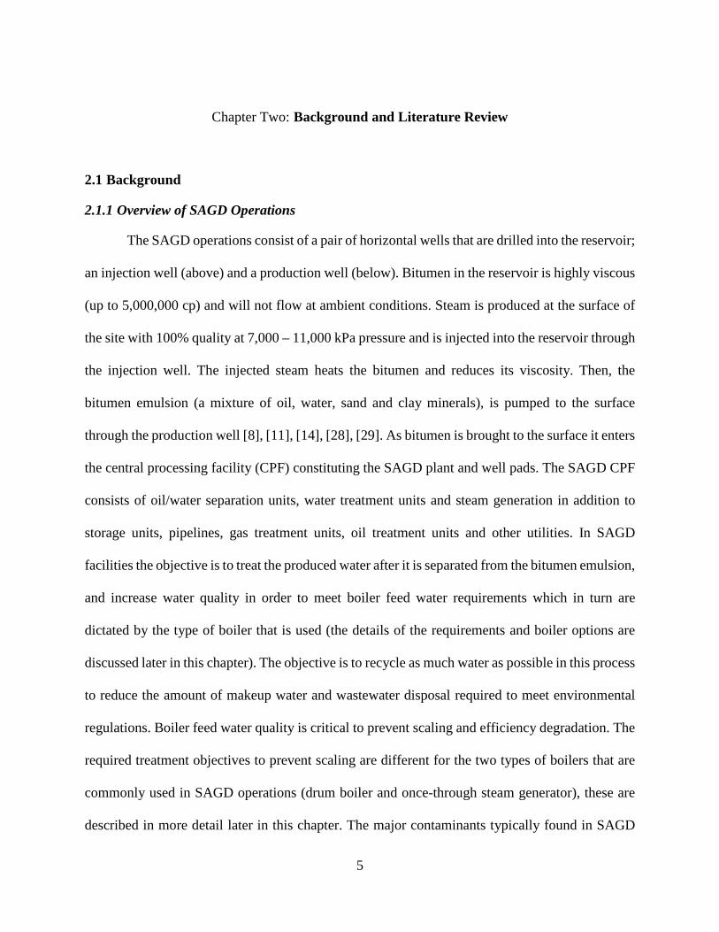
of treatment processes. Figure 2-1 shows SAGD operations schematically and the following is an
overview of the water treatment and steam generation system in SAGD operations, where the
system can be divided into 5 sections shown in Figure 2-1:
7
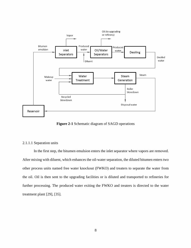
Figure 2-1 Schematic diagram of SAGD operations
2.1.1.1 Separation units
In the first step, the bitumen emulsion enters the inlet separator where vapors are removed.
After mixing with diluent, which enhances the oil-water separation, the diluted bitumen enters two
other process units named free water knockout (FWKO) and treaters to separate the water from
the oil. Oil is then sent to the upgrading facilities or is diluted and transported to refineries for
further processing. The produced water exiting the FWKO and treaters is directed to the water
treatment plant [29], [35].
8

2.1.1.2 Water deoiling
Deoiling is the first step in treating produced water. In the deoiling section of the plant the
remaining free oil that has not already been separated from the water in the separation units is
removed and the oil content in the produced water is reduced from between 1200 and 2000 ppm
to approximately 1 ppm. A variety of deoiling equipment can be employed for oil removal (e.g.,
dissolved or induced gas flotation, filters, membranes, etc.). Oil removal is usually performed in
three steps; primary, secondary and tertiary treatment. In primary treatment or bulk oil removal,
oil is removed from water via gravity separation. A skim tank is commonly used for bulk oil
removal in SAGD facilities, but other types of oil/water separators have been investigated (e.g.,
API separators and the corrugated plate interceptor (CPI) separator [23], [36]). In primary deoiling,
approximately 90% of the oil is separated from the water [23], [36]. Secondary treatment uses air
flotation technologies to separate smaller droplets of oil that are not separated in the first step.
Dissolved or induced gas flotation (DGF/IGF) are common unit operations for secondary oil
separation in SAGD operations. Deoiling hydrocyclones have recently been introduced to oil sands
water treatment activities as a replacement for part of the bulk oil removal and flotation process
[23], [33], [36]–[39]. Hydrocyclones are typically used as a pre-treatment process in conjunction
with other technologies. They do not require chemical inputs, have high tolerance for inlet oil
concentration and it is reported that they have long lifetimes (however, public literature does not
state the specifically this lifetime [39]). Tertiary treatment of oil removal is filtration. Oil removal
filters are used to remove the final traces of oil in the produced water. Walnut shell filters are
commonly used for this step.
9
All deoiling processes introduced above, are capable of removing suspended solids as well.
In primary deoiling, approximately 50% of suspended solids are removed via settling. Gas flotation
and filtration also remove roughly 70% and 90% of suspended solids respectively.
Ceramic membranes are a new deoiling technology that has been evaluated in different
studies to replace either the entire deoiling equipment or the secondary and tertiary oil removal
stages [36], [40]. A ceramic membrane is also capable of removing silica and suspended solids
from wastewater [8], [23], [29], [37], [41].
A summary of deoiling processes and their efficiency in oil removal is shown in Table 2-
3 (data sources [12], [27], [28], [30]).
Table 2-3 Deoiling processes and their oil removal efficiency
Process Separation technology
Oil droplet size
removal
Effluent oil concentration
(ppm)
Approximate removal ratio
Skim tank Gravity > 150 μm 200-400 85-90 %
API separator Gravity > 150 μm 200-400 50-99 %
CPI separator Gravity/Coalescence > 50 μm 100 -*
DGF/IGF Flotation > 20 μm 10-40 90-93 % Deoiling
hydrocyclone Centrifugal force > 10 μm 20-40 90-93%
Filtration Absorption < 2 μm 1-5 90 %
Membrane Barrier < 1 μm 0.5-4 -* *Accurate removal ratios could not be found in the literature.
10

2.1.1.3 Water treatment
Deoiled produced water is sent to the water treatment units to remove the water soluble
contaminants. Soluble contaminants in SAGD produced water include silica, hardness (calcium,
magnesium, iron, etc.), total dissolved solids, organic carbon and dissolved oxygen.
Warm or hot lime softening1 (WLS/HLS) and ion exchange are traditional processes for
silica and hardness removal that have been employed in SAGD operations for decades. These
processes are capable of removing silica and hardness via physical-chemical treatment.
WLS followed by a filtration system, removes silica and part of the hardness (there is a
debate about whether hardness is removed in the lime softening unit in the SAGD water treatment
process). It has been reported that part of the hardness (calcium and magnesium ions concentration)
(about 50%) is removed in the lime softening units [42], [43], but available water quality data for
industrial projects show no change or very small changes in hardness concentration after passing
through the lime softening unit (in this study a zero hardness removal in the lime softening unit is
assumed). The most widely used chemical compounds in this treatment process are calcium
hydroxide (lime, Ca(OH)2) and magnesium oxide (MgO). Sludge is produced during the softening
process and is separated from the treated water by a filter followed by dewatering in a centrifuge.
The sludge handling process is included as a part of the lime softening process in the present study.
The ion exchange unit is typically a weak acid cation exchanger (WAC) that reduces calcium,
magnesium and iron (hardness) content to meet the boiler specifications by using sodium carbonate
1 Warm and hot lime softening are similar regarding the configuration, water recycle, water quality and GHG emissions [24]. In this study WLS is used to represent both processes.
11
(soda ash: Na2CO3). The ion exchange system is regenerated with sodium hydroxide (caustic:
NaOH) and hydrochloric acid (HCl) regularly.
The water quality achieved by this approach meets the specifications for the OTSG but is
not clean enough to be used in a drum boiler. The recycle ratio of produced water using this
approach is approximately 80-90% depending on whether the boiler blowdown is recycled for
further treatment or is completely disposed of [30], [43], [44].
An evaporation method has recently been introduced to SAGD operations as a new water
treatment technology by employing vertical tube, falling film, vapor compression evaporators [45],
[46]. This process eliminates the sludge and some of chemicals required by the WLS or HLS units.
The chemicals required for the evaporative method are sodium hydroxide (caustic, NaOH),
antifoam and scale inhibitor. Caustic is added to increase pH for increasing the silica solubility in
order to avoid scaling in the evaporator. The heat transfer coefficient of vertical tube falling film
evaporators is the highest among all evaporator types. In this process, all dissolved solids are
removed to very low (below 1-2 ppm) concentrations and high quality distillate is generated for
use in the boiler. The quality of the effluent is compatible with standard drum boilers feed water
requirements. The contaminants are removed from the boiler feed water and separated in a waste
stream as evaporator blowdown which is about 1-2 wt% (weight percent) whereas the evaporator
recovers 98-99 wt% of the feed water [30], [43]. Dissolved oxygen is commonly removed from
the boiler feed by oxygen scavenger chemicals such as sodium sulphite or in a thermal deaerator
[8], [23], [47].
12

2.1.1.4 Steam generation
Treated produced water is then used for steam generation that is then injected into the wells.
Two types of boilers are currently used by SAGD operations for steam generation; once-through
steam generators (OTSG) and drum boilers.
OTSGs produce steam with 75-80% quality (not all the feed water vaporizes) and since
100% steam is required, a series of vapor-liquid separators (flash drum) are needed to separate the
water from the steam and produce 100% quality steam for injection. The separated water stream
that is not converted to steam is known as boiler blowdown. Removing this stream from the boiler
helps to control boiler water quality parameters within the required limits to avoid scaling,
corrosion and foaming issues. Boiler blowdown is either recycled back to the treatment system for
further treatment and reuse or sent to disposal (deep well injection or zero liquid discharge - ZLD
crystallizer) so that the contaminants exit the water treatment system [8], [19], [24].
Drum boilers are capable of producing 100% quality steam which eliminates the need for
vapor-liquid separators. Only 1-2% of the boiler feed water in this type of boiler is removed as
blowdown to control boiler water quality parameters. However, this comes at the cost of increased
capital costs and increased consumption of electricity. This is one of the tradeoffs that is explored
in this thesis.
Boiler feed water specifications for the OTSG and drum boiler are shown in Table 2-4 [8],
[19], [23], [32], [47]–[52]. Quality requirements for the OTSG that are reported across the studies
are quite different; therefore, the acceptable range for water quality shown in Table 2-4 is broad.
Drum boilers require lower contaminant concentrations and higher quality in the boiler feed water.
This is due to the higher quality of generated steam in this type of boiler.
13

Table 2-4 Boiler feed water quality requirements for OTSG and drum boiler
Parameter OTSG
requirement (ppm)
References Drum boiler requirement
(ppm) References
Oil 0.5-10 [8], [23], [32], [48], [52] 0.2 [23], [32]
TDS 7,000-12,000 [8], [23], [32], [48], [52] 5 [32]
TSS <1 [32], [52] <1 [32], [47], [49]
Hardness 0.5-1 [8], [19], [23], [32], [48], [52] 0.02-0.5 [19], [23], [32]
Silica 20-150 [8], [19], [23], [32], [48], [52] 0.1-2 [19], [23], [32]
TOC 200-600 [19], [32] 0.2 [19], [32]
DO 0.04 [8], [23], [52] 0.04 [23], [47], [49] Specific
conductance 2,000-10,000* [19] 150* [19], [23]
*Unit is μS/cm
2.1.1.5 Waste disposal
Boiler blowdown and evaporator blowdown are liquid waste streams in the system that are
recycled for treatment and reuse or are disposed of. The type of boiler used for steam generation
determines the amount of boiler blowdown that is generated. OTSG blowdown is approximately
20% of the boiler feed water volume that traditionally is disposed of via deep well injection. Drum
boiler blowdown is only 1-2% of boiler feed water that is disposed of in the same way. The other
method of wastewater disposal is the zero liquid discharge (ZLD) crystallizer which is usually
used in conjunction with an evaporator. ZLD crystallizers eliminate liquid waste completely via a
drying process and generate a distillate stream (pure distilled water) that is recycled back to the
boiler and a solid waste for disposal [43]. The solid waste is an easy-to-handle dry solid that can
be safely disposed of in a landfill [53], [54].
14
2.2 Literature review
2.2.1 Comparison of water treatment processes
Technical and economical comparisons of chemical treatment (i.e., lime softening and ion
exchange) and evaporative treatment methods have been conducted and presented in the academic
literature. Heins et al., Hill et al. and Perdicakis review both treatment methods in their studies and
suggest that there are some advantages of evaporation over the chemical treatment [24], [43], [44],
[55]:
• Using evaporators for water treatment increase process reliability.
• Boiler feed water quality is significantly improved with evaporators and makes the use of
drum boilers possible. Moreover, drum boilers allow for the use of alternate fuels which is
not an option with OTSGs. That is, OTSGs use natural gas to generate steam, but in drum
boilers other types of fuel (e.g., oil) can be used which adds flexibility to the process. Drum
boilers eliminate the need for vapor-liquid separators and reduce the volume of blowdown.
• The evaporative approach requires less chemicals.
• Sludge handling issues are eliminated with evaporators.
• Water recovery is improved and makeup water consumption is decreased.
• Economical evaluations show that the total installed costs for evaporators and drum boilers
are 8-10% lower than the conventional method (lime softening and OTSG).
• Operating costs for the evaporative approach are 1-6% lower than the conventional
approach.
Some advantages of traditional water treatment method from the aforementioned studies
are listed below:
• There is a risk of limiting steam production in case of severe fouling in evaporators.
15

• Cleaning process of drum boilers is more complicated than OTSGs. Drum boilers need
chemical cleaning.
• Boiler feed water quality requirement for drum boilers is higher than OTSGs.
• Energy consumption and GHG emissions in evaporation treatment are higher than
chemical treatment.
The advantages and disadvantages of using ZLD crystallizers have been investigated in
several previous studies. A Jacobs Consultancy report concludes that ZLD increases the produced
water recycle ratio, but at the same time increases energy use, GHG emissions and capital cost in
the process. This study also reports that the use of ZLD complicates the operation and may
decrease the reliability of the system [24]. Lozier et al. reached the same conclusion in their study
[56]. They concluded that the main advantage of using a ZLD system is increased recycle ratio of
the water and the main disadvantage of using such system is high capital and operating cost [56].
The results of a third study on brine-concentrate treatment and disposal options indicated that the
main advantages to a ZLD system is a high quality product water and proven history for use in
industrial applications (but not in the oil sands industry). They concur that the main disadvantages
are high capital, operating and maintenance cost, mechanical complexity of the system and the
need for frequent cleaning [57].
These studies investigate the technical and economic advantages of each approach, but the
potential improvements within each approach have not been considered. That is to say, most of
the studies found in the literature investigate the advantages and disadvantages associated with
replacing a treatment unit or a set of treatment processes with other treatment process alternatives.
This is not sufficient because there is also potential for the diversion of flows to reduce cost and
energy that have not to date been addressed in the literature. In addition, there are further
16

opportunities to explore the explicit evaluation of tradeoffs between decisions that affect energy,
water, cost and GHG emissions.
In Jacobs consultancy report by Hill et al. [24], the impact of increasing the water recycle
ratio and achieving zero liquid discharge (ZLD) on energy use, GHG emissions and waste
generation in SAGD operations is explored. The authors completed over 100 simulations to
evaluate nine different water treating configurations in terms of water use, water recycle, energy
consumption, GHG emissions and waste generation. They tried to keep balance between
environmental tradeoffs and economic returns by identifying the most promising water treatment
technologies. The results of this study revealed that blowdown evaporation best balance
environmental tradeoffs and economic returns. They also concluded that adding new technologies
(e.g., ZLD) that increase the produced water recycle ratio (by 1-2%), will result in an increased
energy use and GHG emissions (by 2-8%). However, the effect of other parameters such as the
performance of the water treatment processes, energy consumption and cost of the treatment units,
etc. (sensitivity analysis) are not investigated in Jacobs study.
It should be noted that the best technology depends on facility specific conditions (e.g.,
produced water and make-up water chemistry), power generation (power from grid vs. natural gas
cogeneration) and how GHG emissions are valued [25].
Process integration tools provide the opportunity to improve water treatment networks by
evaluating alternative configurations of the system without changing the treatment technologies
under consideration and only by rearranging the wastewater streams in the network. None of the
studies described above applied these tools.
Energy and water consumption, cost, waste production and GHG emissions are parameters
that are affected by the choice of treatment process, steam generation and waste disposal method.
17
In the present study, the design of distributed effluent treatment which is a subset of process
integration approaches and optimization techniques are used to provide insights about the
opportunities for improvement of the SAGD operations. In this study, we are interested in applying
a combination of water pinch analysis and optimization tools on the SAGD water treatment
network to investigate the tradeoffs between cost, energy, emissions and water as well as finding
the opportunities to divert wastewater flows around treatment units to improve the water treatment
network.
2.2.2 Process Integration and Pinch Analysis
Process integration is a set of techniques to study the process design and look for
inefficiencies in industrial processes. Process integration is used to assess modifications to
industrial processes to quantify the potential to reduce energy, water and raw material
consumption, GHG emissions and waste generation. Pinch analysis is the most common tool
among process integration techniques because of the simplicity of its primary concept and the
successful use of this method in different industrial projects around the world (e.g. up to 42%
reduction in water use in a refinery plant) [58]–[60]. Process integration, combined with other tools
such as process simulation and optimization, is an efficient (relatively simple to use and effective)
approach to analyze industrial processes and investigate the interactions between different parts of
a system [58], [61], [62].
Two main areas of pinch analysis applications are energy pinch and water pinch. The goal
of energy pinch is to minimize the total energy consumed by a process for heating and cooling by
modifying the heat exchanger network in the process based on process integration rules and
maximizing the heat recovered between process streams. An energy pinch analysis for the SAGD
18
operations suggests that water-energy tradeoffs exist [63], [64]. As a result, the focus of this
research is on analyzing the water network in the SAGD operations using water pinch concepts.
This will allow us to understand the correlation between water and energy and to identify
opportunities to optimize both water and energy use simultaneously by considering these tradeoffs
using specific criteria. Water pinch can be applied to build a water network to achieve two different
goals [65], [66]:
1. Minimizing wastewater generation by water reuse and recycle.
2. Designing a distributed effluent treatment system to treat generated wastewater.
The first application deals with water consuming operations in a facility. The idea is to
minimize fresh water consumption by optimizing water allocation to different operations and
maximizing water reuse or recycle based on the nature of the operations. The second application
evaluates a set of wastewater streams that could be treated for a number of contaminants in several
treatment units with the possibility of partial or total bypass for each unit, in order to reach the
environmental limit for all the contaminants (or any other performance goals).
In the SAGD water cycle, the only water consuming process is below the surface, inside
the reservoir. Since there is no other water consuming unit, there are not many opportunities for
reducing water consumption by using pinch analysis. Adding solvent to improve bitumen
extraction and reduce water consumption is possible, but it requires different types of analyses and
is outside the scope of pinch analysis (adding solvent can reduce water consumption by enhancing
the oil extraction, and is not related to pinch analysis). On the other hand, when water returns to
the surface and is separated from oil, it must be treated and recycled back into the process.
Therefore, the second approach within water pinch analysis can be used to investigate and optimize
water treatment as part of SAGD operations and is the main focus of this study.
19

2.2.3 Distributed effluent treatment system vs. centralized treatment system
Wastewater treatment in industrial plants is commonly carried out in a central treatment
facility where all the effluent streams from various processes that consume fresh water and produce
wastewater (e.g., desalting, washing operations, etc.) are collected in a common sewer and then
are sent through a series of treatment processes to reduce the concentration of different
contaminants to desired levels [66], [67]. Wastewater treatment in SAGD plants is conventionally
carried out in a centralized treatment system. Depending on the contaminant concentrations and
discharge limitations, the centralized treatment system might include primary, secondary and
tertiary treatment processes. A centralized treatment facility is illustrated schematically in Figure
2-2.
Figure 2-2 Centralized treatment plant
20

It has been noted that a distributed effluent treatment system (or segregated wastewater
treatment system) can have important advantages over centralized wastewater treatment [68]–[70].
This is due to the fact that streams can be treated separately and only combined if it is appropriate
according to certain rules that are presented later in this section. Other studies have shown that in
most wastewater treatment operations, the capital and operating costs are proportional to the total
flow rate of wastewater that flows through the treatment unit [66], [67], [71]. Therefore, by
designing a distributed system as shown in Figure 2-3, any wastewater stream can flow to any
treatment unit with the possibility of a partial bypass and with potentially reduced total system
costs/energy consumption.
Figure 2-3 Distributed effluent treatment system
21

Mishra et al. and Tyteca et al. review studies in the area of optimal design of water
treatment systems. Most of these studies that were conducted between 1974 and 1994 focused on
optimizing specific units or small groups of units with a single specific configuration [72], [73].
In these studies fundamental mechanisms that are the target of the wastewater treatment processes,
such as control of bacterial growth, oxygen supply, sedimentation, etc. are mathematically
modeled. Mathematical models are used to find optimal efficiency and cost (maximizing the
efficiency and minimizing the cost) of each unit by changing the size of treatment units or the
process parameters such as contaminant concentrations, water flow rate and temperature (which
are the decision variables of the mathematical model). Then the model is solved to optimize (e.g.
minimize cost or maximize efficiency) a specific system that consists of specific treatment units
arranged in a specific order. The maximum efficiency or the minimum cost is determined by
finding the proper size of treatment units as decision variables. Alternatively, a set of previously
dimensioned process units can be assumed and the optimal order of the units can be determined
via optimization techniques. In these studies only wastewater streams with specific contaminant
concentrations are investigated and they are not practical if the contaminant concentrations or any
of the other input parameters are changed. That is, if the input parameters are changed, the entire
model has to be rebuilt. Therefore, a general approach is needed to optimize water treatment
networks with different sets of input parameters. The suggested approach in the present study
allows for changing any of the input parameters (e.g. contaminant concentrations of the wastewater
streams) without the need to make any changes in the model. Since 1994, various new methods
have been proposed for optimal design of a wastewater treatment system [66], [74]–[77]. The two
main methods that are most applicable in this thesis can be categorized into graphical methods
based on the pinch analysis concept and mathematical modeling approaches.
22
Wang and Smith proposed a general conceptual graphical approach to design a distributed
effluent system for process industries based on the pinch analysis concept [66]. They assumed that
a set of wastewater streams containing specific contaminants are given with known flow rates and
concentrations. Moreover, the environmental concentration limits that must be achieved by the
treatment system are specified. Then, they assumed that a set of treatment processes were available
to remove the contaminants. Performance of the treatment processes were described by a fixed
removal ratio or a fixed outlet concentration for each contaminant in each treatment unit. Another
important assumption in this study is that the total cost of each treatment unit (capital and
operating) is proportionally related to the flow rate of the wastewater stream treated in that unit.
Although the relationship between cost and flow rate could be linear or nonlinear, Wang and Smith
assumed a linear relationship in their study. Therefore, total cost of the treatment system can be
minimized by minimizing the total flow rate of the streams going through the treatment units. To
achieve the optimal design of the system, a two-step method is suggested in this paper. First, the
minimum flow rate of effluent to be treated is set as the target (targeting step). Second, a network
is designed based on a set of design rules to achieve the target flow rate and concentration
requirements (design step).
A simplified description of the targeting and design steps discussed in Wang and Smith
study, for a single stream and single contaminant system is presented here. A wastewater stream
can be represented by considering the relationship between concentration and mass load of the
contaminant as seen in Figure 2-4. The horizontal and vertical axes are mass load and concentration
of the contaminant respectively. The goal of wastewater treatment processes is typically to reduce
the concentration of the contaminant in the waste stream from the inlet concentration (Cin) to the
desired concentration limit (Ce). The contaminant mass load to be removed from the waste stream
23
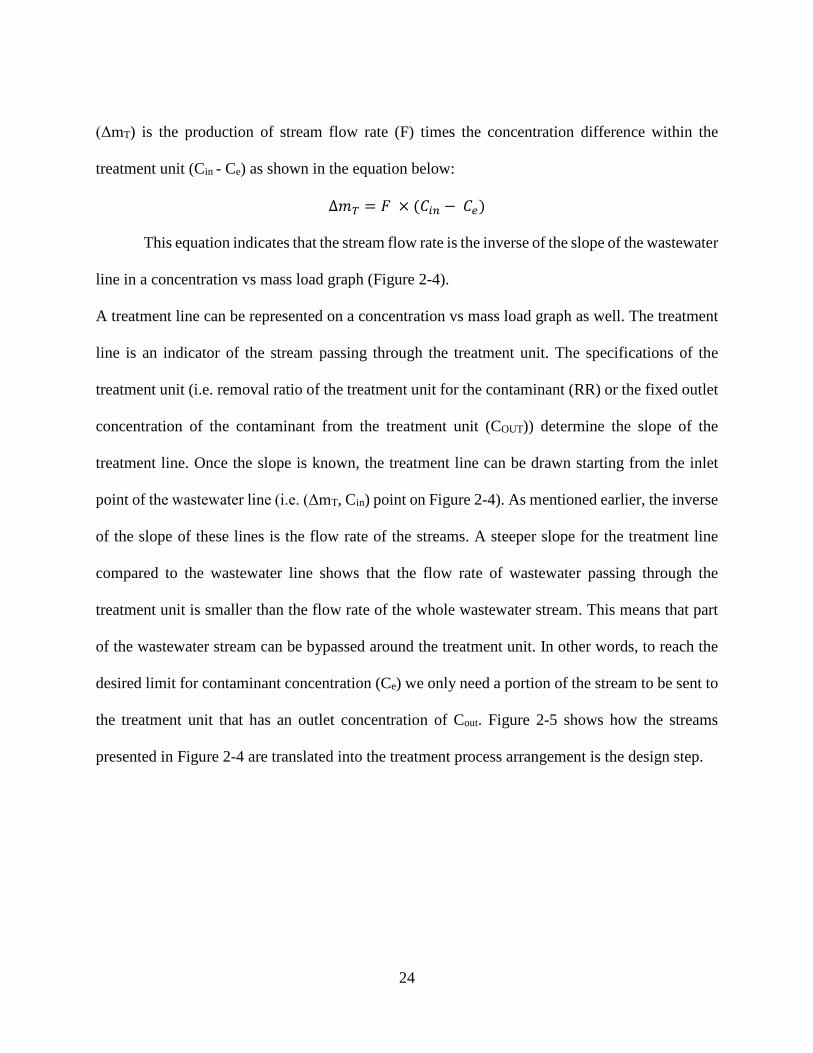
(ΔmT) is the production of stream flow rate (F) times the concentration difference within the
treatment unit (Cin - Ce) as shown in the equation below:
∆𝑚𝑚𝑇𝑇 = 𝐹𝐹 × (𝐶𝐶𝑖𝑖𝑖𝑖 − 𝐶𝐶𝑒𝑒)
This equation indicates that the stream flow rate is the inverse of the slope of the wastewater
line in a concentration vs mass load graph (Figure 2-4).
A treatment line can be represented on a concentration vs mass load graph as well. The treatment
line is an indicator of the stream passing through the treatment unit. The specifications of the
treatment unit (i.e. removal ratio of the treatment unit for the contaminant (RR) or the fixed outlet
concentration of the contaminant from the treatment unit (COUT)) determine the slope of the
treatment line. Once the slope is known, the treatment line can be drawn starting from the inlet
point of the wastewater line (i.e. (ΔmT, Cin) point on Figure 2-4). As mentioned earlier, the inverse
of the slope of these lines is the flow rate of the streams. A steeper slope for the treatment line
compared to the wastewater line shows that the flow rate of wastewater passing through the
treatment unit is smaller than the flow rate of the whole wastewater stream. This means that part
of the wastewater stream can be bypassed around the treatment unit. In other words, to reach the
desired limit for contaminant concentration (Ce) we only need a portion of the stream to be sent to
the treatment unit that has an outlet concentration of Cout. Figure 2-5 shows how the streams
presented in Figure 2-4 are translated into the treatment process arrangement is the design step.
24
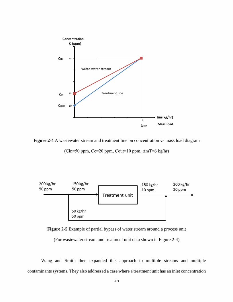
Figure 2-4 A wastewater stream and treatment line on concentration vs mass load diagram
(Cin=50 ppm, Ce=20 ppm, Cout=10 ppm, ΔmT=6 kg/hr)
Figure 2-5 Example of partial bypass of water stream around a process unit
(For wastewater stream and treatment unit data shown in Figure 2-4)
Wang and Smith then expanded this approach to multiple streams and multiple
contaminants systems. They also addressed a case where a treatment unit has an inlet concentration
25
limit. Detailed information about these methods are found in [66]. Although the general approach
proposed by Wang and Smith offers valuable insights into the design of the distributed effluent
treatment system, there are shortcomings associated with this method. Because of the graphical
nature of the targeting step, this method is able to manage only simple design constraints and is
not an efficient approach for problems with a large number of treatment units and contaminants as
a result of interactions that occur between treatment processes and contaminants. In some cases,
this approach is not capable of predicting the lowest possible target flow rate in multiple-unit,
multi-contaminant problems. This is discussed further in the Kuo and Smith paper [67].
Additionally, to deal with systems involving two or more treatment units capable of removing a
specific contaminant, decisions need to be made about the mass load distribution of the
contaminant and the sequence of treatment units. These decisions might lead to suboptimal
network designs.
Kuo and Smith improved the earlier method by addressing the important features of
multiple treatment processes system design and existing interactions in an industrial water system
that were neglected in the previous study [78]. They proposed a staged graphical approach by
repeating the targeting and design steps. This method does not guarantee the minimum flow rate
but guides the designer towards the optimal design [67]. Kuo and Smith divided the water system
of an industrial plant into three subsystems: the water-using subsystem, the regeneration subsystem
and the effluent treatment subsystem. However, there are drawbacks associated with this method
as well. For example, although they addressed the design procedure of a distributed effluent
treatment for systems with three wastewater streams and three contaminants, because the
composite curves and network structure are constructed manually, this method is likely to fail
when used for systems with larger number of contaminants and treatment units (i.e. the method
26

might not be able to solve the problem or might give incorrect results). Also, because there are
strong interactions between these subsystems, Kuo and Smith method that divides the water system
into three separate subsystems, fails to explore all of the interactions. Furthermore, the final design
achieved by this method depends on the designer’s experience and may not be consistent. In other
words, one designer might make one set of decisions and another designer a different set of
decisions (i.e., when one contaminant is removed by more than one treatment unit, decisions must
be made about the load of contaminant in each treatment unit and the order of treatment units).
Another problem with this method and the method proposed by Wang and Smith is that they cannot
easily accommodate constraints to the design other than concentration and flow rate constraints,
such as limiting constraints for the distance between two treatment units, the size of treatment units
and avoiding uneconomically small flow rates between treatment units (it is not economic to set
up additional pipelines to transfer small flows. The proposed model in the present study is capable
of accepting constraints, e.g. a lower bound on the stream flow rates to avoid these small flows).
Mathematical optimization methods have gained attention in the past two decades [74]–
[76], [79]. Mathematical design techniques for the synthesis of distributed effluent treatment
networks usually depend on the solution of nonconvex mathematical models which lead to
multiple local optimal points and often cause local optimization techniques to fail [79]. In 1980,
Takama et al. developed an optimization approach and applied it in a petroleum refinery [80]. The
initial problem is a large dimensional and nonlinear problem with strict inequality constraints.
They transformed the model into a set of problems with no inequality constraints by applying a
penalty function. Then, the simplified models were solved using the “Complex” method [81]. In
this study which is one of the first studies investigating the optimal design of a water treatment
network with the aid of mathematical programming, optimization techniques are used to solve a
27

simple problem far from the real systems and it is not expanded to a general problem of optimal
water treatment network design. The expansion of the proposed method in Takama study will
require additional mathematical tools which make it impossible to expand the suggested solution
without making fundamental changes and rebuilding their model.
In 1988, Galan and Grossmann proposed a procedure based on linear underestimators that
was introduced by Quesada and Grossmann for bilinear terms within a branch and bound
algorithm, for solving the mixed integer nonlinear problem resulting from modeling a distributed
effluent treatment system [74], [82]. The proposed model in this paper gives rise to a nonconvex
nonlinear problem that usually causes convergence complications. Accordingly, the authors
successfully used linear underestimators to turn the initial nonlinear problem into a set of relaxed
linear models which provide initialization points for the original nonlinear problem [74]. This
method is useful in cases with the possibility of estimating tight linear relaxations for the bilinear
terms of the nonlinear problem. In cases similar to the present study where accurate linear
estimations cannot be made before solving the nonlinear problem, the use of linear relaxation
cannot help solving the initial nonlinear problem.
Hernández-Suárez et al. proposed a superstructure decomposition and parametric
optimization approach for the synthesis of a distributed wastewater treatment network [79]. In the
proposed method, the design search space is subdivided into smaller pieces by dividing the typical
complex network superstructure into a series of simple network superstructures. Then, the optimal
network design related to each simple superstructure is determined by solving a set of linear
programming models that is derived from the initial nonconvex model by fixing a number of
variables. This method is suitable for the systems with three treatment units or less.
28
Alva-Argáez et al. proposed an integrated approach based on the pinch analysis concept
for the design of industrial water systems within a mathematical programming model framework
[76], [83]. The proposed superstructure includes all possible reuse, recycle, regeneration and
treatment options in the system. A feasible solution of the original MINLP (mixed-integer
nonlinear programming) model is obtained by decomposing the MINLP model into a MILP and
LP problems and solving them iteratively. In the proposed method, the objective function of the
MILP model is augmented by an infeasibility term with an increasing coefficient that targets a
reduction of the problem infeasibilities. This method takes into account a more complete set of
constraints and treatment units which make it flexible to be used for a large number of treatment
units and contaminants. Therefore, a similar approach is used in the present study.
Liu et al. proposed a new heuristic procedure to obtain the optimal design of distributed
effluent treatment system by reducing unnecessary stream-mixing [77]. The proposed approach is
applied to multi-stream, multi-contaminant systems with more than two treatment units. Although
this approach addresses the problems of dealing with a large number of treatment units and
contaminants, the heuristic nature of the procedure could lead to different configurations of
streams in the final design depending on the designers’ judgement.
Process integration methods using mathematical programming tools have not been applied
to oil sands processes and specifically SAGD operations before. In this study, set of different
concepts and tools across the literature are incorporated and blended in order to develop a
comprehensive model that can handle a large set of possible process units, contaminants, etc. In
addition, different treatment options across a set of metrics (cost, energy, GHG emissions, etc.)
are compared. In this thesis, the details of the SAGD system (including the parameters of the
SAGD water treatment processes such as removal ratios, effluent concentration, cost, etc.) are
29
represented within a model that applies process integration techniques. Additionally, sensitivity
analysis is conducted to assess the impact of changing several input parameters on the output
parameters of the optimization model.
30

Chapter Three: Methods
3.1 Objective of the model
The mathematical model developed in this study is designed to minimize energy
consumption and cost of the water treatment network in SAGD operations. Environmental
regulations for water withdrawal, water disposal and GHG emissions [18], [27] challenge oil
producers to recycle as much produced water as possible in the extraction process and competition
in a global market encourages them to minimize energy consumption and cost per unit oil
produced. There are tradeoffs between cost, energy and water consumption in a water treatment
network. The model that is designed and implemented in this study uses optimization techniques
to evaluate all three factors simultaneously to explore these tradeoffs. In other words, the model is
designed to reach an optimal water treatment network, such that process constraints and
environmental limits are met at minimum cost and/or energy consumed.
One way to potentially reduce the cost and energy use in a treatment system is to design a
distributed effluent treatment system instead of a centralized treatment system. Several studies
applied in other industries have shown that distributed effluent treatment can have significant
advantages over centralized wastewater treatment [66], [80], [84]–[86]. These studies also reveal
that the capital cost of most wastewater treatment operations is proportional to the total flow of
wastewater through the system. Therefore, by designing a distributed system that can reduce flow
through particular units, there is potential to reduce the capital cost of the system.
Design of a distributed effluent system has been successfully applied in various industries
(e.g., petroleum refinery, pulp and paper industries, textile and dairy plants [67], [75], [80], [87]),
but has not been used in SAGD operations before. So, in this study cost, energy and water saving
31

opportunities in a SAGD water treatment network using process integration and optimization tools
are explored.
3.2 Operations Research and Mathematical Modeling
Operations research (OR) is a scientific tool and an interdisciplinary branch of applied
mathematics that helps researchers in the decision making process and uses mathematical
modeling, statistics and algorithms to find the best design of a system that is usually associated
with allocation of scarce resources. A “system” is defined as a set of interdependent components
that work together to reach the goal of the system. [88], [89].
A mathematical model is used to represent an actual system with mathematical equations.
The decision making process using the scientific approach of OR usually involves one or more
mathematical models. From a practical perspective, OR can be defined as an optimization process
that aims to find the minimum or maximum of an objective function. A general OR model can be
represented by the following general format:
Maximize or minimize Objective Function
Subject to
Constraints
3.2.1 Objective function
In most models there is a function we want to be maximized or minimized, this function is
called the objective function of the model. The most common objective functions in optimization
problems are profit, cost, energy, loss, time, yield and risk [88], [90], [91].
32
3.2.2 Decision variables
Decision variables are independent variables that are controlled by the user and influence
the constraints and the objective value [88].
3.2.3 Constraints
Constraints are the process model and describe the interrelationships of the key variables
of the system that are represented in the form of mathematical equations. Formulating the problem
is the main step in the optimization process and requires identifying the essential elements of a
system and present them mathematically [88], [91].
Constraints of a mathematical programming model can be an equality or inequality:
𝑒𝑒𝑒𝑒𝑒𝑒𝑒𝑒𝑒𝑒𝑒𝑒𝑒𝑒𝑒𝑒 𝑐𝑐𝑐𝑐𝑐𝑐𝑐𝑐𝑒𝑒𝑐𝑐𝑒𝑒𝑒𝑒𝑐𝑐𝑒𝑒:𝑔𝑔(𝑥𝑥) = 0
𝑒𝑒𝑐𝑐𝑒𝑒𝑒𝑒𝑒𝑒𝑒𝑒𝑒𝑒𝑒𝑒𝑒𝑒𝑒𝑒 𝑐𝑐𝑐𝑐𝑐𝑐𝑐𝑐𝑒𝑒𝑐𝑐𝑒𝑒𝑒𝑒𝑐𝑐𝑒𝑒:ℎ1(𝑥𝑥) ≥ 0 𝑐𝑐𝑐𝑐 ℎ2(𝑥𝑥) ≤ 0
In the standard form of a linear programming (LP) model, all constraints are equality
constraints. To convert inequality constraints to equality constraints, slack and surplus variables
are used.
ℎ1(𝑥𝑥) ≥ 0 → ℎ1(𝑥𝑥) − 𝑐𝑐1 = 0
ℎ2(𝑥𝑥) ≤ 0 → ℎ2(𝑥𝑥) + 𝑐𝑐2 = 0
𝑐𝑐1 is called a surplus variable and is a positive value. By subtracting a surplus variable a
“≥” constraint is converted into a “=” constraint. 𝑐𝑐2 is called a slack variable and is positive too.
By adding a slack variable, a “≤” constraint is converted into a “=” constraint.
33
3.2.4 Feasible region and optimal solution
A feasible solution of an optimization problem is a set of values for decision variables that
satisfies all the constraints of the model. The feasible region of a problem constitutes all possible
feasible solutions to that problem. An optimal solution of a problem is the feasible solution that
gives the best (minimum or maximum) value of the objective function among all feasible solutions
[88], [90].
3.2.5 Linear and nonlinear models
If all the constraints and the objective function of an optimization model are first degree
functions of decision variables, it is a linear model. If an optimization model is not linear, i.e. the
objective function of the model or one or more constraints of the model are second degree or higher
functions of decision variables, then it is a nonlinear programming problem.
3.2.6 Integer and non-integer models
If one or more decision variables assume integer values, the optimization model is an
integer model. If all the decision variables are continuous and free to have fractional values, the
optimization model is a non-integer model.
3.2.7 Convex and nonconvex sets
In optimization problems, the feasible region forms a convex set if the line segment
connecting any pair of distinct feasible points lies entirely inside the set. If a set is not convex, it
is a nonconvex set [88], [90], [91]. Simple examples of convex and nonconvex sets are shown in
Figure 3-1.
34

The feasible region of linear models are always convex sets, but nonlinear models can be
convex or nonconvex. Integer models are always nonconvex [88], [90].
3.3 Overview of the model
The proposed model explores different wastewater treatment and steam generation options
for SAGD operations. The conceptual design of the system is based on process integration and
pinch analysis concepts. Water treatment units and wastewater streams are the main components
of the system. The mathematical representation of the system is built based on the system
superstructure that is described in the next section and leads to a mixed-integer nonlinear
programming model (MINLP) with a cost/energy objective function. The MINLP problem is
divided into two simpler sub-models; mixed-integer linear programming (MILP) and linear
programming (LP) models, by introducing a penalty function and projection and relaxation
approaches. An iterative method is used to find the optimal solution of the MILP model, minimum
cost/energy and optimal flow rates. These results are then fed to the MINLP model to ensure the
decomposition has not missed major design features.
The model consists of mass balance equations for a set of treatment units and several
process constraints for treatment units and other components of the system such as splitters and
Convex set Nonconvex set
Figure 3-1 Examples of convex and nonconvex sets
35

mixers to ensure the feasibility of the system and satisfy the concentration and flow rate limits of
the treatment units. A number of different scenarios are investigated that will be explained in the
next section in detail. For each scenario, the model is solved to minimize both energy and cost
functions separately. Then all scenarios are compared in terms of cost, energy and water
consumption and the tradeoffs between them are investigated to determine the magnitude of the
divergence, the nature of the tradeoffs are explained, thresholds are determined, etc.
3.4 Problem description
3.4.1 Overview of the system components
The optimization model is designed as a system consisting of a set of wastewater streams
containing contaminants with known flow rates and concentrations and a number of treatment
units with known performance parameters (e.g., removal ratios), cost and energy consumption.
The performance of each treatment unit can either be specified by a fixed outlet concentration or
a fixed removal ratio for each contaminant. Each treatment unit is capable of removing one or
more contaminants from the wastewater stream. A general rule of thumb that is used throughout
industry [66] is that the cost of a treatment unit is a direct function of the flow rate of the wastewater
stream passing through that unit.
There are three main liquid streams in the system; one stream of wastewater (produced
water), a makeup water stream and boiler blowdown. Flow rate and contaminant concentrations
of these streams are different for different SAGD projects. However, for a specific SAGD plant
the flow rate and contaminant concentrations for each of these streams are known or can be
calculated from the parameters (e.g., quality of produced steam from steam generator and flow
losses in the treatment units) of the system. Produced water specifications are defined by the
36

production rate of the SAGD project and the reservoir characteristics and can be input by the user.
Flow rate and concentration of boiler blowdown vary based on the type of boiler used for steam
generation and the disposal method and is explained in detail later in this chapter. Makeup water
flow rate depends on the flow rate of produced water and boiler blowdown. Its contaminant
concentrations depend on the water source used to supply makeup water. The concentration of
contaminants in the makeup water stream is assumed to be known in my system.
The main contaminants in the waste streams of the system are oil, silica, metal ions
(Calcium, Magnesium, etc. that can be represented as total hardness (TH)), total organic carbon
(TOC), total suspended solids (TSS) and total dissolved solids (TDS). The aforementioned
contaminants can be removed from wastewater streams using various treatment processes
considered in this model. Some of the treatment processes are currently used by industry (e.g.,
skim tank, induced gas flotation, oil removal filter, warm/hot lime softening, ion exchange, and
evaporator) and some are being explored (e.g., ceramic membrane and hydrocyclone).
Contaminant concentrations of the produced water stream, fresh and brackish makeup
water that are used in the optimization model are shown in Table 3-1. Available treatment
processes along with the main contaminants they can remove are summarized in Table 3-2.
37
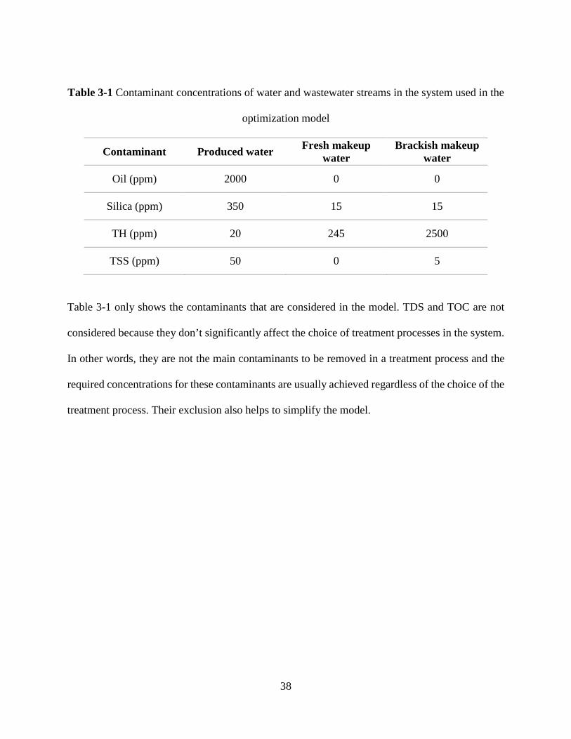
Table 3-1 Contaminant concentrations of water and wastewater streams in the system used in the
optimization model
Contaminant Produced water Fresh makeup water
Brackish makeup water
Oil (ppm) 2000 0 0
Silica (ppm) 350 15 15
TH (ppm) 20 245 2500
TSS (ppm) 50 0 5
Table 3-1 only shows the contaminants that are considered in the model. TDS and TOC are not
considered because they don’t significantly affect the choice of treatment processes in the system.
In other words, they are not the main contaminants to be removed in a treatment process and the
required concentrations for these contaminants are usually achieved regardless of the choice of the
treatment process. Their exclusion also helps to simplify the model.
38

Table 3-2 Treatment processes and removable contaminants in SAGD operations
Treatment process Contaminants
Skim tank (ST) Oil
Induced gas flotation (IGF) Oil
Oil removal filter (ORF) Oil
Hydrocyclone (HC) Oil
Warm/Hot lime softening (WLS/HLS) Silica, Hardness
Weak acid cation exchanger (WAC) Hardness
Evaporator (Evap) Silica, Hardness
Ceramic membrane (CM) Oil, Suspended solids, Silica
Table 3-2 shows some treatment processes can only remove one contaminant and some are
capable of removing more than one contaminant. All the treatment processes listed in Table 3-2
are considered in the model except hydrocyclone and ceramic membrane, since not enough
information about the performance of these treatment processes is available in the literature. More
importantly, these treatment processes have yet to be deployed by the SAGD industry. However
the methodology described in this work could incorporate these and other novel technologies as
data becomes available.
Performance parameters of the treatment units (i.e., fixed outlet concentration and fixed
removal ratio) are available in the literature [37], [42], [92]. The mathematical model can use either
of the parameters (fixed outlet concentration and fixed removal ratio) to solve the optimization
39
problem. Also, industry specific data were obtained and used in this study under a confidentiality
agreement.
Two key parameters of the system that are used in the mathematical representation of the
system, are defined and explained here to provide a better link between the treatment processes
introduced earlier with the parameters of the system:
3.4.1.1 Contaminant mass load:
Contaminant mass load (the amount of mass of the contaminant) in a wastewater stream is
the mass flow rate of that contaminant in the stream. Mass load of contaminant c in wastewater
stream i is defined as:
𝑀𝑀𝑐𝑐,𝑖𝑖 = 𝐹𝐹𝑖𝑖 ∗ 𝐶𝐶𝑐𝑐,𝑖𝑖 3.1
Where:
𝑀𝑀𝑐𝑐,𝑖𝑖 is the mass load of contaminant c in wastewater stream i,
𝐹𝐹𝑖𝑖 is the flow rate of wastewater stream i, and
𝐶𝐶𝑐𝑐,𝑖𝑖 is the concentration of contaminant c in wastewater stream i
3.4.1.2 Removal ratio:
Removal ratio is the percentage of a contaminant mass load in a wastewater stream that is
removed by a treatment unit and can be shown as:
𝑅𝑅𝑅𝑅𝑐𝑐,𝑡𝑡𝑡𝑡 =𝐹𝐹𝑡𝑡𝑡𝑡𝑖𝑖𝑖𝑖 ∗ 𝐶𝐶𝑐𝑐,𝑡𝑡𝑡𝑡
𝑖𝑖𝑖𝑖 − 𝐹𝐹𝑡𝑡𝑡𝑡𝑜𝑜𝑡𝑡𝑡𝑡 ∗ 𝐶𝐶𝑐𝑐,𝑡𝑡𝑡𝑡𝑜𝑜𝑡𝑡𝑡𝑡
𝐹𝐹𝑡𝑡𝑡𝑡𝑖𝑖𝑖𝑖 ∗ 𝐶𝐶𝑐𝑐,𝑡𝑡𝑡𝑡𝑖𝑖𝑖𝑖 =
𝑀𝑀𝑐𝑐,𝑡𝑡𝑡𝑡𝑖𝑖𝑖𝑖 − 𝑀𝑀𝑐𝑐,𝑡𝑡𝑡𝑡
𝑜𝑜𝑡𝑡𝑡𝑡 𝑀𝑀𝑐𝑐,𝑡𝑡𝑡𝑡𝑖𝑖𝑖𝑖 3.2
40
Where:
𝑅𝑅𝑅𝑅𝑐𝑐,𝑡𝑡𝑡𝑡 is the removal ratio of contaminant c in treatment unit tu,
𝐹𝐹𝑡𝑡𝑡𝑡𝑖𝑖𝑖𝑖 and 𝐹𝐹𝑡𝑡𝑡𝑡𝑜𝑜𝑡𝑡𝑡𝑡are the flow rates of inlet and outlet streams of treatment unit tu respectively,
𝐶𝐶𝑐𝑐,𝑡𝑡𝑡𝑡𝑖𝑖𝑖𝑖 and 𝐶𝐶𝑐𝑐,𝑡𝑡𝑡𝑡
𝑜𝑜𝑡𝑡𝑡𝑡 are the concentration of contaminant c in inlet and outlet streams of treatment unit
tu respectively,
𝑀𝑀𝑐𝑐,𝑡𝑡𝑡𝑡𝑖𝑖𝑖𝑖 and 𝑀𝑀𝑐𝑐,𝑡𝑡𝑡𝑡
𝑜𝑜𝑡𝑡𝑡𝑡 are the mass load of contaminant c entering and exiting the treatment unit tu
respectively.
The goal of a wastewater treatment system is to reach specific concentration limits for
various contaminants (e.g. environmental limits for wastewater disposal). All outlet streams from
treatment units within the central processing facility are combined at a discharge point and the
concentration of all contaminants in this combined stream should be within the required
concentration limits. In this work, the desired concentrations of the contaminants are determined
by boiler feed water requirements which in turn are defined by the type of boiler in operation. This
means that once the type of boiler is selected (between OTSG and drum boiler, before running the
optimization model) the target contaminant concentrations required for treated water are
established.
The goal of the optimization problem is to reach the optimal design of the treatment system.
The optimal design determines the treatment units that are selected, the streams that move through
each treatment unit and the streams that connect the treatment units to satisfy concentration
requirements at the final discharge point at the lowest cost and/or level of energy consumption.
The SAGD wastewater treatment and steam generation system is shown schematically in
Figure 3-2.
41
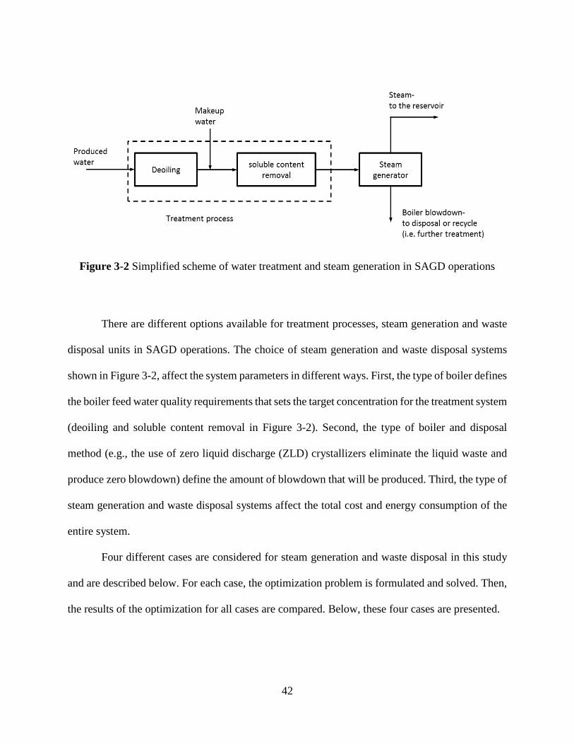
Figure 3-2 Simplified scheme of water treatment and steam generation in SAGD operations
There are different options available for treatment processes, steam generation and waste
disposal units in SAGD operations. The choice of steam generation and waste disposal systems
shown in Figure 3-2, affect the system parameters in different ways. First, the type of boiler defines
the boiler feed water quality requirements that sets the target concentration for the treatment system
(deoiling and soluble content removal in Figure 3-2). Second, the type of boiler and disposal
method (e.g., the use of zero liquid discharge (ZLD) crystallizers eliminate the liquid waste and
produce zero blowdown) define the amount of blowdown that will be produced. Third, the type of
steam generation and waste disposal systems affect the total cost and energy consumption of the
entire system.
Four different cases are considered for steam generation and waste disposal in this study
and are described below. For each case, the optimization problem is formulated and solved. Then,
the results of the optimization for all cases are compared. Below, these four cases are presented.
42
3.4.1.3 Four cases for steam generation and waste disposal system in SAGD operations
Four cases for the combination of steam generation and waste disposal methods in the
SAGD operations were analyzed in order to explore the energy/cost implications associated with
different technologies considered by industry.
Case 1- OTSG, no blowdown recycle: In the first case, an OTSG is assumed to be used
for steam generation. OTSGs generate approximately 75-80% quality steam2 [8] and OTSG
blowdown is assumed not to be recycled for further treatment and is disposed of via deep well
injection.
Case 2- OTSG, blowdown evaporation: In this case, again an OTSG is used for steam
generation and OTSG blowdown is sent to an evaporator for further treatment. Evaporator
distillate is then used as boiler feed water.
Case 3- OTSG, 30% blowdown recycle: In this case, again an OTSG is used for steam
generation. However, 30% of the OTSG blowdown is recycled back to the water treatment system
for further treatment and the remaining is disposed of via deep well injection.
Case 4- Drum boiler: In the fourth case, a drum boiler is assumed to be used for steam
generation. Drum boilers generate close to 100% quality steam and the amount of produced
blowdown is very small.
In both cases 2 and 3 OTSG blowdown is sent to treatment processes for further treatment,
but the difference between these two cases is that in case 2, the OTSG blowdown is forced to be
treated in an evaporator and the selection of the blowdown stream and blowdown evaporator are
not part of the optimization problem. In case 3 the blowdown stream is one of the wastewater
2 In this study I assumed 80% quality steam is generated in OTSG.
43
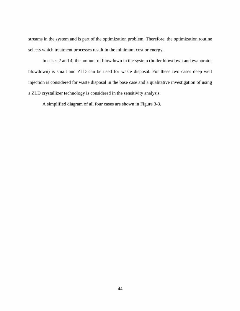
streams in the system and is part of the optimization problem. Therefore, the optimization routine
selects which treatment processes result in the minimum cost or energy.
In cases 2 and 4, the amount of blowdown in the system (boiler blowdown and evaporator
blowdown) is small and ZLD can be used for waste disposal. For these two cases deep well
injection is considered for waste disposal in the base case and a qualitative investigation of using
a ZLD crystallizer technology is considered in the sensitivity analysis.
A simplified diagram of all four cases are shown in Figure 3-3.
44
Figure 3-3 Four cases for steam generation and waste disposal in SAGD operations
45
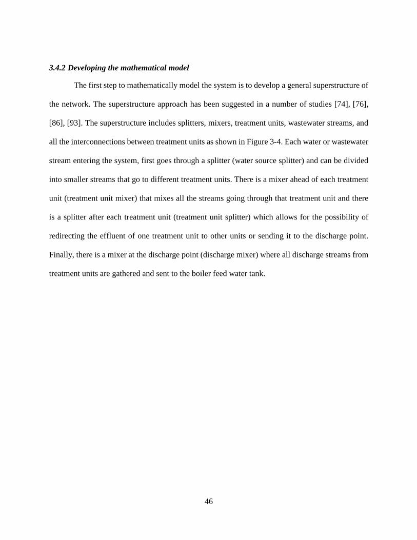
3.4.2 Developing the mathematical model
The first step to mathematically model the system is to develop a general superstructure of
the network. The superstructure approach has been suggested in a number of studies [74], [76],
[86], [93]. The superstructure includes splitters, mixers, treatment units, wastewater streams, and
all the interconnections between treatment units as shown in Figure 3-4. Each water or wastewater
stream entering the system, first goes through a splitter (water source splitter) and can be divided
into smaller streams that go to different treatment units. There is a mixer ahead of each treatment
unit (treatment unit mixer) that mixes all the streams going through that treatment unit and there
is a splitter after each treatment unit (treatment unit splitter) which allows for the possibility of
redirecting the effluent of one treatment unit to other units or sending it to the discharge point.
Finally, there is a mixer at the discharge point (discharge mixer) where all discharge streams from
treatment units are gathered and sent to the boiler feed water tank.
46
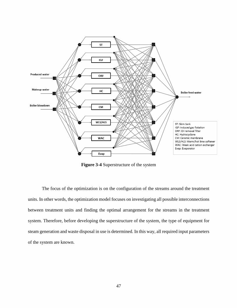
Figure 3-4 Superstructure of the system
The focus of the optimization is on the configuration of the streams around the treatment
units. In other words, the optimization model focuses on investigating all possible interconnections
between treatment units and finding the optimal arrangement for the streams in the treatment
system. Therefore, before developing the superstructure of the system, the type of equipment for
steam generation and waste disposal in use is determined. In this way, all required input parameters
of the system are known.
47

The next step is defining the cost/energy relationships for each treatment unit as a function
of flow rate. In this study a linear correlation3 between cost/energy and flow rate is assumed.
𝐶𝐶𝑐𝑐𝑐𝑐𝑒𝑒/𝐸𝐸𝑐𝑐𝑒𝑒𝑐𝑐𝑔𝑔𝑒𝑒 = 𝑒𝑒 ∗ 𝐹𝐹𝑒𝑒𝑐𝑐𝐹𝐹𝑐𝑐𝑒𝑒𝑒𝑒𝑒𝑒 + 𝑏𝑏 3.3
Where “a” and “b” are fixed coefficients and are determined based on the type of the treatment
unit.
In the mathematical model, the objective function may be the total cost of the system, or
total energy consumption. Constraints in the model are mainly mass balance equations and some
additional constraints of the system that are explained later. Decision variables are stream flow
rates through each treatment unit. This means that the model will try to find the minimum possible
value for the objective function by exploring all possible combinations of flow rates through each
treatment unit, while all equality and inequality constraints are satisfied. Then, the system is
mathematically modeled based on the system superstructure shown in Figure 3-4. Before
representing the system in the form of mathematical equations, variables and parameters along
with the components of the system used in mathematical equations need to be defined. Sets,
variables and parameters of the model are presented below.
3.4.2.1 Sets, parameters and variables
Sets
C = {c | c is a contaminant}
c = O Oil,
3 The relationship between flow rate and cost/energy depends on the type of treatment process. Since there is very little information about this relationship for different treatment processes in the literature, a linear relationship is assumed based on the limited data we could gain access through our industrial partners.
48

S Silica,
TH Total hardness,
TDS Total dissolved solids,
TOC Total organic carbon
TU = {tu | tu is a treatment unit}
tu = ST Skim tank,
API API separator,
IGF Induced gas flotation,
DGF Dissolved gas flotation,
ORF Oil removal filter,
HCY Hydro-cyclone,
WLS Warm lime softener,
HLS Hot lime softener,
EVAP Evaporator,
WAC Weak acid cation exchanger,
CM Ceramic membrane
S = {s | s is a water source}
s = PW Produced water,
MUW Makeup water,
BBD Boiler blowdown
Parameters
Flow rates
𝐹𝐹𝑠𝑠 Flow rate of water source s ∈ S
49

𝐹𝐹𝑡𝑡𝑡𝑡𝑙𝑙𝑜𝑜𝑠𝑠𝑠𝑠 Flow loss in treatment unit tu ∈ TU
𝐹𝐹𝐵𝐵𝐵𝐵𝐵𝐵 Boiler feed water flow rate
Concentrations
𝐶𝐶𝑠𝑠,𝑐𝑐 Concentration of contaminant c ∈ C in water stream s ∈ S
𝐶𝐶𝑡𝑡𝑡𝑡,𝑐𝑐𝑜𝑜𝑡𝑡𝑡𝑡,𝑓𝑓𝑖𝑖𝑓𝑓 Fixed outlet concentration of contaminant c ∈ C from treatment unit tu ∈ TU
𝐶𝐶𝑡𝑡𝑡𝑡,𝑐𝑐𝑖𝑖𝑖𝑖,𝑚𝑚𝑚𝑚𝑓𝑓 Maximum allowable inlet concentration of contaminant c ∈ C to treatment unit
tu ∈ TU
𝐶𝐶𝑡𝑡𝑡𝑡,𝑐𝑐𝑙𝑙𝑜𝑜𝑠𝑠𝑠𝑠 Contaminant c concentration of stream that is lost in treatment unit tu ∈ TU
𝐶𝐶𝑐𝑐𝑡𝑡𝑚𝑚𝑡𝑡𝑡𝑡𝑒𝑒𝑡𝑡 Target concentration required at discharge
𝐶𝐶𝑠𝑠,𝑡𝑡𝑡𝑡,𝑐𝑐 Concentration of contaminant c ∈ C in the stream between water source s ∈ S and
treatment unit tu ∈ TU
𝐶𝐶𝑐𝑐𝑚𝑚𝑎𝑎𝑒𝑒 Average concentration of contaminant c ∈ C in the system
Mass loads
𝑀𝑀𝑀𝑀𝑐𝑐𝑡𝑡𝑒𝑒𝑚𝑚 Mass load of contaminant c ∈ C to be removed from the system
𝑀𝑀𝑀𝑀𝑐𝑐𝑡𝑡𝑜𝑜𝑡𝑡 Total mass load of contaminant c ∈ C in the system
Cost parameters
𝐶𝐶𝑐𝑐𝑐𝑐𝑒𝑒𝑠𝑠𝑎𝑎𝑚𝑚𝑡𝑡 Variable cost of water stream s ∈ S
𝐶𝐶𝑐𝑐𝑐𝑐𝑒𝑒𝑠𝑠𝑓𝑓𝑖𝑖𝑓𝑓 Fixed cost of water stream s ∈ S
𝐶𝐶𝑐𝑐𝑐𝑐𝑒𝑒𝑡𝑡𝑡𝑡𝑎𝑎𝑚𝑚𝑡𝑡 Variable cost of treatment unit tu ∈ TU
50
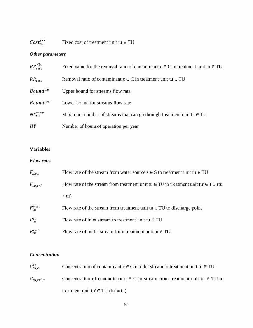
𝐶𝐶𝑐𝑐𝑐𝑐𝑒𝑒𝑡𝑡𝑡𝑡𝑓𝑓𝑖𝑖𝑓𝑓 Fixed cost of treatment unit tu ∈ TU
Other parameters
𝑅𝑅𝑅𝑅𝑡𝑡𝑡𝑡,𝑐𝑐𝑓𝑓𝑖𝑖𝑓𝑓 Fixed value for the removal ratio of contaminant c ∈ C in treatment unit tu ∈ TU
𝑅𝑅𝑅𝑅𝑡𝑡𝑡𝑡,𝑐𝑐 Removal ratio of contaminant c ∈ C in treatment unit tu ∈ TU
𝐵𝐵𝑐𝑐𝑒𝑒𝑐𝑐𝐵𝐵𝑡𝑡𝑢𝑢 Upper bound for streams flow rate
𝐵𝐵𝑐𝑐𝑒𝑒𝑐𝑐𝐵𝐵𝑙𝑙𝑜𝑜𝑙𝑙 Lower bound for streams flow rate
𝑁𝑁𝑁𝑁𝑡𝑡𝑡𝑡𝑚𝑚𝑚𝑚𝑓𝑓 Maximum number of streams that can go through treatment unit tu ∈ TU
𝐻𝐻𝐻𝐻 Number of hours of operation per year
Variables
Flow rates
𝐹𝐹𝑠𝑠,𝑡𝑡𝑡𝑡 Flow rate of the stream from water source s ∈ S to treatment unit tu ∈ TU
𝐹𝐹𝑡𝑡𝑡𝑡,𝑡𝑡𝑡𝑡ˊ Flow rate of the stream from treatment unit tu ∈ TU to treatment unit tuʹ ∈ TU (tuʹ
≠ tu)
𝐹𝐹𝑡𝑡𝑡𝑡𝑒𝑒𝑓𝑓𝑖𝑖𝑡𝑡 Flow rate of the stream from treatment unit tu ∈ TU to discharge point
𝐹𝐹𝑡𝑡𝑡𝑡𝑖𝑖𝑖𝑖 Flow rate of inlet stream to treatment unit tu ∈ TU
𝐹𝐹𝑡𝑡𝑡𝑡𝑜𝑜𝑡𝑡𝑡𝑡 Flow rate of outlet stream from treatment unit tu ∈ TU
Concentration
𝐶𝐶𝑡𝑡𝑡𝑡,𝑐𝑐𝑖𝑖𝑖𝑖 Concentration of contaminant c ∈ C in inlet stream to treatment unit tu ∈ TU
𝐶𝐶𝑡𝑡𝑡𝑡,𝑡𝑡𝑡𝑡´,𝑐𝑐 Concentration of contaminant c ∈ C in stream from treatment unit tu ∈ TU to
treatment unit tuʹ ∈ TU (tuʹ ≠ tu)
51

𝐶𝐶𝑡𝑡𝑡𝑡,𝑐𝑐𝑒𝑒𝑓𝑓𝑖𝑖𝑡𝑡 Concentration of contaminant c ∈ C in the stream from treatment unit tu ∈ TU to
the discharge point
𝐶𝐶𝑡𝑡𝑡𝑡,𝑐𝑐𝑜𝑜𝑡𝑡𝑡𝑡 Outlet concentration of contaminant c ∈ C from treatment unit tu ∈ TU
𝐶𝐶𝑐𝑐𝐵𝐵𝐵𝐵𝐵𝐵 Discharge concentration of contaminant c ∈ C (at discharge point)
Mass load
𝑀𝑀𝑀𝑀𝑡𝑡𝑡𝑡,𝑐𝑐𝑡𝑡𝑒𝑒𝑚𝑚 Mass load of contaminant c ∈ C that is removed in treatment unit tu ∈ TU specified
with a fixed outlet concentration
𝑀𝑀𝑀𝑀𝑡𝑡𝑡𝑡,𝑐𝑐𝑖𝑖𝑖𝑖 Mass load of contaminant c ∈ C entering the treatment unit tu ∈ TU
𝑀𝑀𝑀𝑀𝑡𝑡𝑡𝑡,𝑐𝑐𝑜𝑜𝑡𝑡𝑡𝑡 Mass load of contaminant c ∈ C exiting the treatment unit tu ∈ TU
𝑀𝑀𝑀𝑀𝑡𝑡𝑡𝑡,𝑐𝑐𝑡𝑡𝑚𝑚𝑖𝑖𝑖𝑖 Slack variable for mass load of contaminant c ∈ C in treatment unit tu ∈ TU
𝑀𝑀𝑀𝑀𝑡𝑡𝑡𝑡,𝑐𝑐𝑙𝑙𝑜𝑜𝑠𝑠𝑠𝑠 Surplus variable for mass load of contaminant c ∈ C in treatment unit tu ∈ TU
Cost and energy variables
𝐶𝐶𝑐𝑐𝑐𝑐𝑒𝑒𝑡𝑡𝑡𝑡𝑡𝑡𝑜𝑜𝑡𝑡 Total cost of treatment unit tu ∈ TU
𝐶𝐶𝑐𝑐𝑐𝑐𝑒𝑒𝑜𝑜𝑢𝑢 Operating cost of the system
𝐶𝐶𝑐𝑐𝑐𝑐𝑒𝑒𝑐𝑐𝑚𝑚𝑢𝑢 Capital cost of the system
𝐶𝐶𝑐𝑐𝑐𝑐𝑒𝑒𝑡𝑡𝑜𝑜𝑡𝑡 Total cost of the system
𝑒𝑒𝑐𝑐𝑒𝑒𝑐𝑐𝑔𝑔𝑒𝑒𝑡𝑡𝑡𝑡𝑎𝑎𝑚𝑚𝑡𝑡 Total energy consumption of the system
Some of the parameters such as the flow rate and concentration of water sources (except
the flow rate of the makeup water stream), performance parameters of treatment units (fixed outlet
concentration or removal ratio), maximum tolerable concentration entering treatment units, cost
52

parameters and target concentrations at the discharge point, are input manually from data sources
available in the literature or from industrial data sources. Other parameters (e.g., the flowrate of
makeup water stream, mass load of contaminant removed in each treatment unit, etc.) are
calculated from the known parameters that are input manually as mentioned above. The parameters
that are calculated are presented below and in the following section.
3.4.2.2 Constraints
Constraints of the problem are as follows:
Overall mass balance4
�𝐹𝐹𝑠𝑠𝑠𝑠
− 𝐹𝐹𝐵𝐵𝐵𝐵𝐵𝐵 = �𝐹𝐹𝑡𝑡𝑡𝑡𝑙𝑙𝑜𝑜𝑠𝑠𝑠𝑠𝑡𝑡𝑡𝑡
3.4
(See Figure 3-5)
4 All mass balance equations are for water.
53

Figure 3-5 Overall mass balance in the system
Mass balance around splitters and mixers
𝐹𝐹𝑠𝑠 = �𝐹𝐹𝑠𝑠,𝑡𝑡𝑡𝑡𝑡𝑡𝑡𝑡
∀ 𝑐𝑐 ∈ 𝑁𝑁 3.5
Equation 3.5 shows the mass balance for the water source splitters where each water source can
be sent to one or more treatment units. See Figure 3-6.
Figure 3-6 Mass balance for the water source splitters
54

�𝐹𝐹𝑠𝑠,𝑡𝑡𝑡𝑡 + �𝐹𝐹𝑡𝑡𝑡𝑡ʹ,𝑡𝑡𝑡𝑡𝑡𝑡𝑡𝑡ʹ
= 𝐹𝐹𝑡𝑡𝑡𝑡𝑖𝑖𝑖𝑖𝑠𝑠
∀ 𝑒𝑒𝑒𝑒 ∈ 𝑇𝑇𝑇𝑇 3.6
𝐹𝐹𝑡𝑡𝑡𝑡𝑜𝑜𝑡𝑡𝑡𝑡 = �𝐹𝐹𝑡𝑡𝑡𝑡,𝑡𝑡𝑡𝑡ʹ𝑡𝑡𝑡𝑡ʹ
+ 𝐹𝐹𝑡𝑡𝑡𝑡𝑒𝑒𝑓𝑓𝑖𝑖𝑡𝑡 ∀ 𝑒𝑒𝑒𝑒 ∈ 𝑇𝑇𝑇𝑇 3.7
Equations 3.6 and 3.7 show the mass balance around the treatment unit mixer and splitter
respectively. As shown in Figure 3-7 the inlet stream to each treatment unit is the combination of
the water sources that are sent to the unit and the recycled streams from other treatment units to
that unit. The outlet stream from each treatment unit can be divided into recycled streams to other
treatment units and a discharge stream.
Figure 3-7 Mass balance for the treatment unit mixers and splitters
�𝐹𝐹𝑡𝑡𝑡𝑡𝑒𝑒𝑓𝑓𝑖𝑖𝑡𝑡𝑡𝑡𝑡𝑡
= 𝐹𝐹𝐵𝐵𝐵𝐵𝐵𝐵 3.8
Equation 3.8 shows the mass balance for the discharge mixer. All discharge streams are
collected together and mixed at the discharge point (see Figure 3-8).
55

Figure 3-8 Mass balance for the discharge mixer
Mass balance around treatment units
𝐹𝐹𝑡𝑡𝑡𝑡𝑖𝑖𝑖𝑖 − 𝐹𝐹𝑡𝑡𝑡𝑡𝑜𝑜𝑡𝑡𝑡𝑡 = 𝐹𝐹𝑡𝑡𝑡𝑡𝑙𝑙𝑜𝑜𝑠𝑠𝑠𝑠 ∀ 𝑒𝑒𝑒𝑒 ∈ 𝑇𝑇𝑇𝑇 3.9
Equations 3.9 shows the mass balance for the total flow through each treatment unit (see
Figure 3-7, dashed boundary line).
Component mass balance in each treatment unit
�1 − 𝑅𝑅𝑅𝑅𝑡𝑡𝑡𝑡,𝑐𝑐� ∗ 𝑀𝑀𝑀𝑀𝑡𝑡𝑡𝑡,𝑐𝑐𝑖𝑖𝑖𝑖 − 𝑀𝑀𝑀𝑀𝑡𝑡𝑡𝑡,𝑐𝑐
𝑜𝑜𝑡𝑡𝑡𝑡 − 𝐹𝐹𝑡𝑡𝑡𝑡𝑙𝑙𝑜𝑜𝑠𝑠𝑠𝑠 ∗ 𝐶𝐶𝑡𝑡𝑡𝑡,𝑐𝑐𝑙𝑙𝑜𝑜𝑠𝑠𝑠𝑠 = 0 ∀ 𝑒𝑒𝑒𝑒 ∈ 𝑇𝑇𝑇𝑇 , 𝑐𝑐 ∈ 𝐶𝐶 3.10
𝑀𝑀𝑀𝑀𝑡𝑡𝑡𝑡,𝑐𝑐𝑖𝑖𝑖𝑖 − 𝑀𝑀𝑀𝑀𝑡𝑡𝑡𝑡,𝑐𝑐
𝑜𝑜𝑡𝑡𝑡𝑡 − 𝑀𝑀𝑀𝑀𝑡𝑡𝑡𝑡,𝑐𝑐𝑡𝑡𝑒𝑒𝑚𝑚 − 𝐹𝐹𝑡𝑡𝑡𝑡𝑙𝑙𝑜𝑜𝑠𝑠𝑠𝑠 ∗ 𝐶𝐶𝑡𝑡𝑡𝑡,𝑐𝑐
𝑙𝑙𝑜𝑜𝑠𝑠𝑠𝑠 = 0 ∀ 𝑒𝑒𝑒𝑒 ∈ 𝑇𝑇𝑇𝑇 , 𝑐𝑐 ∈ 𝐶𝐶 3.11
Equations 3.10 and 3.11 show the mass balance for each contaminant in each treatment
unit when the performance of the treatment unit is specified by a fixed removal ratio and a fixed
outlet concentration respectively.
56

Part of the inlet stream might be lost from the system during each treatment process. 𝐹𝐹𝑡𝑡𝑡𝑡𝑙𝑙𝑜𝑜𝑠𝑠𝑠𝑠
and 𝐶𝐶𝑡𝑡𝑡𝑡,𝑐𝑐𝑙𝑙𝑜𝑜𝑠𝑠𝑠𝑠 are the flow rate and the concentration of the lost stream in each treatment unit
respectively. 𝐹𝐹𝑡𝑡𝑡𝑡𝑙𝑙𝑜𝑜𝑠𝑠𝑠𝑠 is estimated for each treatment unit based on the nature of the process and 𝐶𝐶𝑡𝑡𝑡𝑡,𝑐𝑐𝑙𝑙𝑜𝑜𝑠𝑠𝑠𝑠
depends on the type of the process and can be estimated based on the type of the operation and
inlet and outlet concentrations.
Definition of inlet and outlet mass loads of contaminant c in treatment units
𝑀𝑀𝑀𝑀𝑡𝑡𝑡𝑡,𝑐𝑐𝑖𝑖𝑖𝑖 and 𝑀𝑀𝑀𝑀𝑡𝑡𝑡𝑡,𝑐𝑐
𝑜𝑜𝑡𝑡𝑡𝑡 are the inlet and outlet mass loads of each contaminant for each
treatment unit respectively. These two terms are used in Equations 3.10 and 3.11 and are defined
as:
��𝐹𝐹𝑡𝑡𝑡𝑡ʹ,𝑡𝑡𝑡𝑡 ∗ 𝐶𝐶𝑡𝑡𝑡𝑡,𝑐𝑐𝑜𝑜𝑡𝑡𝑡𝑡 �
𝑡𝑡𝑡𝑡ʹ
+ ��𝐹𝐹𝑠𝑠,𝑡𝑡𝑡𝑡 ∗ 𝐶𝐶𝑠𝑠,𝑐𝑐�𝑠𝑠
− 𝑀𝑀𝑀𝑀𝑡𝑡𝑡𝑡,𝑐𝑐𝑖𝑖𝑖𝑖 = 0 ∀ 𝑒𝑒𝑒𝑒 ∈ 𝑇𝑇𝑇𝑇 , 𝑐𝑐 ∈ 𝐶𝐶 3.12
𝐶𝐶𝑡𝑡𝑡𝑡,𝑐𝑐𝑜𝑜𝑡𝑡𝑡𝑡 ∗ ��𝐹𝐹𝑡𝑡𝑡𝑡ʹ,𝑡𝑡𝑡𝑡
𝑡𝑡𝑡𝑡ʹ
+ �𝐹𝐹𝑠𝑠,𝑡𝑡𝑡𝑡𝑠𝑠
− 𝐹𝐹𝑡𝑡𝑡𝑡𝑙𝑙𝑜𝑜𝑠𝑠𝑠𝑠� − 𝑀𝑀𝑀𝑀𝑡𝑡𝑡𝑡,𝑐𝑐𝑜𝑜𝑡𝑡𝑡𝑡 = 0 ∀ 𝑒𝑒𝑒𝑒 ∈ 𝑇𝑇𝑇𝑇, 𝑐𝑐 ∈ 𝐶𝐶 3.13
Concentration limit for inlet stream to treatment units
Some treatment units have specific limits for inlet concentration of contaminants and
cannot tolerate high concentrations of one or more contaminants. To avoid violating the
concentration limit Equation 3.14 is added as a constraint.
57

𝑀𝑀𝑀𝑀𝑡𝑡𝑡𝑡,𝑐𝑐𝑖𝑖𝑖𝑖 ≤ 𝐶𝐶𝑡𝑡𝑡𝑡,𝑐𝑐
𝑖𝑖𝑖𝑖,𝑚𝑚𝑚𝑚𝑓𝑓 ∗ 𝐹𝐹𝑡𝑡𝑡𝑡𝑖𝑖𝑖𝑖 ∀ 𝑒𝑒𝑒𝑒 ∈ 𝑇𝑇𝑇𝑇, 𝑐𝑐 ∈ 𝐶𝐶 3.14
Discharge concentration limit to meet boiler feed water quality requirements
Since the purpose of the treatment system is to reach final concentration requirements
(which is the boiler feed water requirements in my study) for all contaminants Equation 3.15 is
added to satisfy the concentration requirements.
��𝐹𝐹𝑡𝑡𝑡𝑡𝑒𝑒𝑓𝑓𝑖𝑖𝑡𝑡 ∗ 𝐶𝐶𝑡𝑡𝑡𝑡,𝑐𝑐𝑜𝑜𝑡𝑡𝑡𝑡�
𝑡𝑡𝑡𝑡
≤ 𝐶𝐶𝑐𝑐𝑡𝑡𝑚𝑚𝑡𝑡𝑡𝑡𝑒𝑒𝑡𝑡 ∗ �𝐹𝐹𝑡𝑡𝑡𝑡𝑒𝑒𝑓𝑓𝑖𝑖𝑡𝑡
𝑡𝑡𝑡𝑡
∀ 𝑐𝑐 ∈ 𝐶𝐶 3.15
Total mass load of contaminant c to be removed from the system
Total mass load of each contaminant that is removed in all treatment units in the system
must be equal to or greater than the minimum mass load that is required to be removed from the
wastewater streams in order to reach the concentration requirements at the discharge point. This
constraint is shown in Equation 3.16.
�𝑀𝑀𝑀𝑀𝑡𝑡𝑡𝑡,𝑐𝑐𝑡𝑡𝑒𝑒𝑚𝑚
𝑡𝑡𝑡𝑡
+ ��𝑅𝑅𝑅𝑅𝑡𝑡𝑡𝑡,𝑐𝑐 ∗ 𝑀𝑀𝑀𝑀𝑡𝑡𝑡𝑡,𝑐𝑐𝑖𝑖𝑖𝑖 �
𝑡𝑡𝑡𝑡
≥ 𝑀𝑀𝑀𝑀𝑐𝑐𝑡𝑡𝑒𝑒𝑚𝑚 ∀ 𝑐𝑐 ∈ 𝐶𝐶 3.16
𝑀𝑀𝑀𝑀𝑐𝑐𝑡𝑡𝑒𝑒𝑚𝑚 is the total mass load of contaminant c that is required to be removed from the
system and is defined as:
𝑀𝑀𝑀𝑀𝑐𝑐𝑡𝑡𝑒𝑒𝑚𝑚 = �𝐹𝐹𝑠𝑠 ∗ (𝐶𝐶𝑠𝑠,𝑐𝑐 − 𝐶𝐶𝑐𝑐𝑡𝑡𝑚𝑚𝑡𝑡𝑡𝑡𝑒𝑒𝑡𝑡)
𝑠𝑠
∀ 𝑐𝑐 ∈ 𝐶𝐶 3.17
58

Cost of treatment units
The cost of each treatment unit consists of a fixed cost (that can be zero) and a variable
cost that is a function of flow rate as shown in Equation 3.18.
𝐶𝐶𝑐𝑐𝑐𝑐𝑒𝑒𝑡𝑡𝑡𝑡𝑡𝑡𝑜𝑜𝑡𝑡 = 𝐶𝐶𝑐𝑐𝑐𝑐𝑒𝑒𝑡𝑡𝑡𝑡𝑎𝑎𝑚𝑚𝑡𝑡 ∗ 𝐹𝐹𝑡𝑡𝑡𝑡𝑖𝑖𝑖𝑖 + 𝐶𝐶𝑐𝑐𝑐𝑐𝑒𝑒𝑡𝑡𝑡𝑡𝑓𝑓𝑖𝑖𝑓𝑓 ∀ 𝑒𝑒𝑒𝑒 ∈ 𝑇𝑇𝑇𝑇 3.18
3.4.2.3 Objective function
The objective function of this problem is the total cost and/or total energy consumption of
the system and they are trying to be minimized. The total cost of the system includes capital cost
and operating cost. Capital cost is assumed to be the cost of treatment units and their installation.
Other expenses such as pumping, piping, etc. are not considered because they are assumed to be
roughly the same for all configurations considered. This assumption was supported through
consultation with industry experts [94]. The operating cost is the sum of treatment units’ expenses
during operation (e.g. electricity consumption of the treatment units, chemicals consumption, etc.)
and the cost of the makeup water stream. Since linear correlations are assumed for cost and energy,
the objective function is represented as a linear expression.
𝑂𝑂𝐹𝐹𝑐𝑐𝑜𝑜𝑠𝑠𝑡𝑡 = �𝐶𝐶𝑐𝑐𝑐𝑐𝑒𝑒𝑡𝑡𝑡𝑡𝑡𝑡𝑜𝑜𝑡𝑡𝑡𝑡𝑡𝑡
+ 𝐻𝐻𝐻𝐻 ∗ �(𝐹𝐹𝑠𝑠 ∗ 𝐶𝐶𝑐𝑐𝑐𝑐𝑒𝑒𝑠𝑠𝑎𝑎𝑚𝑚𝑡𝑡 )𝑠𝑠
3.19
𝑂𝑂𝐹𝐹𝑐𝑐𝑜𝑜𝑠𝑠𝑡𝑡 Objective function for total cost
59
The objective function for total energy consumed is similar to total cost, except energy is
only consumed during operation of the system and in treatment units. Energy consumed during
construction and any indirect or upstream energy consumption is neglected in this model.
𝑂𝑂𝐹𝐹𝑒𝑒𝑖𝑖𝑒𝑒𝑡𝑡𝑡𝑡𝑒𝑒 = ��𝑒𝑒𝑐𝑐𝑒𝑒𝑐𝑐𝑔𝑔𝑒𝑒𝑡𝑡𝑡𝑡𝑎𝑎𝑚𝑚𝑡𝑡 ∗ 𝐹𝐹𝑡𝑡𝑡𝑡𝑖𝑖𝑖𝑖�𝑡𝑡𝑡𝑡
3.20
Energy is consumed for steam generation and waste disposal as well, but since the steam
generator and waste handling equipment are not in the scope of the optimization and are considered
separately in the total cost calculations, these energy terms are not included in the objective
function. Similarly, the cost of the boiler and waste disposal are not considered in the cost objective
function.
For each steam generation and waste disposal combination (introduced earlier in this
chapter) cost and energy of steam generation and waste disposal are calculated separately and are
added to the final optimized cost and energy to arrive at a final total cost estimate for each
combination.
Hereafter, the cost objective function is used when describing the solution steps of the
optimization problem. However, the procedure is identical when the energy objective function is
selected.
The mathematical model described above is a nonlinear problem (NLP). Nonlinearities are
in the form of bilinear terms in equations 3.12, 3.13, and 3.15 where both flow rate and
concentration are unknown variables.
60

Binary variables can be used to show the existence or non-existence of water streams and
treatment units and to assign upper and lower bounds to the streams flow rates. When a treatment
unit is selected in the optimal design of the treatment system, the binary variable associated with
that treatment unit assumes the value of “1”, and if a treatment unit is not selected in the optimal
design, the binary variable associated with that treatment unit assumes the value of “0”. Similarly,
if the flow rate of a stream in the treatment network is nonzero, the binary variable associated with
that stream is “1” and if the flow rate of a stream in the treatment network is zero, the binary
variable associated with that stream is “0”.
By adding binary variables that are introduced below, the problem is converted to a mixed-
integer non-linear (MINLP) problem.
3.4.2.4 Binary variables
𝐵𝐵𝑠𝑠,𝑡𝑡𝑡𝑡 Binary variable to show the existence (value of 1) or non-existence (value of 0) of
the stream from water source s ∈ S to treatment unit tu ∈ TU
𝐵𝐵𝑡𝑡𝑡𝑡,𝑡𝑡𝑡𝑡ʹ Binary variable to show the existence (value of 1) or non-existence (value of 0) of
the stream from treatment unit tu ∈ TU to treatment unit tuʹ ∈ TU
𝐵𝐵𝑡𝑡𝑡𝑡𝑒𝑒𝑓𝑓𝑖𝑖𝑡𝑡 Binary variable to show the existence (value of 1) or non-existence (value of 0) of
the stream from treatment unit tu ∈ TU to discharge point
𝐵𝐵𝑡𝑡𝑡𝑡 Binary variable to show the existence (value of 1) or non-existence (value of 0) of
treatment unit tu ∈ TU
Additional constraints including binary variables are presented here. These constraints
control the reasonableness and practicality (e.g., eliminating the cycles between two treatment
units, avoiding very small flow rates, etc.) of the system.
61

3.4.2.5 Additional constraints (with binary variables)
Eliminating the cycles
This constraint is used to ensure that only one recycled stream exists between two particular
treatment units. In other words, if there is a stream recycled from treatment unit tu to treatment
unit tuʹ, there won’t be any stream recycled from treatment unit tuʹ to treatment unit tu.
𝐵𝐵𝑡𝑡𝑡𝑡,𝑡𝑡𝑡𝑡ʹ + 𝐵𝐵𝑡𝑡𝑡𝑡ʹ,𝑡𝑡𝑡𝑡 ≤ 1 ∀ 𝑒𝑒𝑒𝑒 𝑒𝑒𝑐𝑐𝐵𝐵 𝑒𝑒𝑒𝑒ʹ ∈ 𝑇𝑇𝑇𝑇 (𝑒𝑒𝑒𝑒 ≠ 𝑒𝑒𝑒𝑒ʹ) 3.21
Assigning upper bounds to the streams flow rate
A maximum flow rate can exist in the system and is the sum of all inlet streams (water
sources). The maximum possible flow rate and associated constraints for different streams in the
system are shown in Equations 3.22 to 3.26.
𝐵𝐵𝑐𝑐𝑒𝑒𝑐𝑐𝐵𝐵𝑡𝑡𝑢𝑢 = �𝐹𝐹𝑠𝑠𝑠𝑠
3.22
𝐹𝐹𝑠𝑠,𝑡𝑡𝑡𝑡 − 𝐵𝐵𝑠𝑠,𝑡𝑡𝑡𝑡 ∗ 𝐵𝐵𝑐𝑐𝑒𝑒𝑐𝑐𝐵𝐵𝑡𝑡𝑢𝑢 ≤ 0 ∀ 𝑒𝑒𝑒𝑒 ∈ 𝑇𝑇𝑇𝑇, 𝑐𝑐 ∈ 𝑁𝑁 3.23
𝐹𝐹𝑡𝑡𝑡𝑡,𝑡𝑡𝑡𝑡ʹ − 𝐵𝐵𝑡𝑡𝑡𝑡,𝑡𝑡𝑡𝑡ʹ ∗ 𝐵𝐵𝑐𝑐𝑒𝑒𝑐𝑐𝐵𝐵𝑡𝑡𝑢𝑢 ≤ 0 ∀ 𝑒𝑒𝑒𝑒 𝑒𝑒𝑐𝑐𝐵𝐵 𝑒𝑒𝑒𝑒ʹ ∈ 𝑇𝑇𝑇𝑇 3.24
𝐹𝐹𝑡𝑡𝑡𝑡𝑒𝑒𝑓𝑓𝑖𝑖𝑡𝑡 − 𝐵𝐵𝑡𝑡𝑡𝑡𝑒𝑒𝑓𝑓𝑖𝑖𝑡𝑡 ∗ 𝐵𝐵𝑐𝑐𝑒𝑒𝑐𝑐𝐵𝐵𝑡𝑡𝑢𝑢 ≤ 0 ∀ 𝑒𝑒𝑒𝑒 ∈ 𝑇𝑇𝑇𝑇 3.25
𝐹𝐹𝑡𝑡𝑡𝑡𝑖𝑖𝑖𝑖 − 𝐵𝐵𝑡𝑡𝑡𝑡 ∗ 𝐵𝐵𝑐𝑐𝑒𝑒𝑐𝑐𝐵𝐵𝑡𝑡𝑢𝑢 ≤ 0 ∀ 𝑒𝑒𝑒𝑒 ∈ 𝑇𝑇𝑇𝑇 3.26
62

Assigning lower bounds to stream flow rate
To avoid unreasonably low flow rates (based on the experiences of industry experts [94])
in each stream, a minimum flow rate is defined based on the system specifications and used as the
lower bound of each stream flow rate in the system. The lower bound constraints are shown in
Equations 3.27 to 3.30.
𝐹𝐹𝑠𝑠,𝑡𝑡𝑡𝑡 − 𝐵𝐵𝑠𝑠,𝑡𝑡𝑡𝑡 ∗ 𝐵𝐵𝑐𝑐𝑒𝑒𝑐𝑐𝐵𝐵𝑙𝑙𝑜𝑜𝑙𝑙 ≥ 0 ∀ 𝑒𝑒𝑒𝑒 ∈ 𝑇𝑇𝑇𝑇, 𝑐𝑐 ∈ 𝑁𝑁 3.27
𝐹𝐹𝑡𝑡𝑡𝑡,𝑡𝑡𝑡𝑡ʹ − 𝐵𝐵𝑡𝑡𝑡𝑡,𝑡𝑡𝑡𝑡ʹ ∗ 𝐵𝐵𝑐𝑐𝑒𝑒𝑐𝑐𝐵𝐵𝑙𝑙𝑜𝑜𝑙𝑙 ≥ 0 ∀ 𝑒𝑒𝑒𝑒 𝑒𝑒𝑐𝑐𝐵𝐵 𝑒𝑒𝑒𝑒ʹ ∈ 𝑇𝑇𝑇𝑇 3.28
𝐹𝐹𝑡𝑡𝑡𝑡𝑒𝑒𝑓𝑓𝑖𝑖𝑡𝑡 − 𝐵𝐵𝑡𝑡𝑡𝑡𝑒𝑒𝑓𝑓𝑖𝑖𝑡𝑡 ∗ 𝐵𝐵𝑐𝑐𝑒𝑒𝑐𝑐𝐵𝐵𝑙𝑙𝑜𝑜𝑙𝑙 ≥ 0 ∀ 𝑒𝑒𝑒𝑒 ∈ 𝑇𝑇𝑇𝑇 3.29
𝐹𝐹𝑡𝑡𝑡𝑡𝑖𝑖𝑖𝑖 − 𝐵𝐵𝑡𝑡𝑡𝑡 ∗ 𝐵𝐵𝑐𝑐𝑒𝑒𝑐𝑐𝐵𝐵𝑙𝑙𝑜𝑜𝑙𝑙 ≥ 0 ∀ 𝑒𝑒𝑒𝑒 ∈ 𝑇𝑇𝑇𝑇 3.30
Bounding constraints (3.23 to 3.30) help simplify the optimization problem by directing
the model to search through a smaller range of values for the flow rates throughout the system.
Maximum number of streams going through a treatment unit
�𝐵𝐵𝑠𝑠,𝑡𝑡𝑡𝑡𝑠𝑠
+ �𝐵𝐵𝑡𝑡𝑡𝑡ʹ,𝑡𝑡𝑡𝑡𝑡𝑡𝑡𝑡ʹ
≤ 𝑁𝑁𝑁𝑁𝑡𝑡𝑡𝑡𝑚𝑚𝑚𝑚𝑓𝑓 ∀ 𝑒𝑒𝑒𝑒 ∈ 𝑇𝑇𝑇𝑇 3.31
63
Constraint 3.31 limits the number of wastewater streams that can go through each treatment
unit. This constraint helps simplify the final configuration and makes the final optimal design more
applicable in the industrial plants.
The MINLP model is a non-convex nonlinear optimization problem that is similar to the
formulation presented by Quesada and Grossmann [82]. In this type of problem, the use of MINLP
solvers can lead to erroneous results and global optimality is not guaranteed. In addition, results
of the optimization are highly dependent on the initialization of variables [82], [84], [95], [96].
Therefore, proper initial values are essential to find the global optimum. For this reason a two-step
iterative approach is used to solve the problem. This is described in the next section.
3.5 Solution strategy
Conceptual approaches presented in various studies and mathematical optimization tools
form the basis of the solution strategy in this study [65]–[67], [76], [86], [97]. Quesada and
Grossmann proposed a branch and bound algorithm to solve the optimization problem related to a
contaminant separation network (similar to the problem in this study). The proposed method uses
linear underestimators5 for the bilinear terms to find the global optimum [82]. Galan and
Grossmann introduced a relaxation approach along with linear underestimators that was mentioned
above to solve a distributed effluent treatment problem [74]. They proposed a linear relaxation of
the initial nonlinear problem based on linear underestimators of the nonconvex constraints that
provides a valid lower bound for the global optimum of the initial problem. The relaxed LP is then
solved to minimize the flow rate through a specific treatment unit and the result is used as an initial
5 They used linear functions that were a lower bound for the actual nonlinear constraints in the model.
64

point for the nonlinear problem. This procedure is repeated for each treatment unit and the best
solution (minimum value for the objective function) for the nonlinear problem is selected as the
optimal design. This method is extended to a procedure for the selection of treatment technologies
where the contaminants are removed by mutually exclusive technologies (where a particular
contaminant can be removed in one particular treatment unit). Alva-Argaez proposed a more
general approach where the treatment units are not mutually exclusive, i.e. a particular contaminant
can be removed in more than one treatment unit [93].
The solution strategy in the present study consists of a decomposition approach that was
initially proposed by Alva-Argaez [76], [93]. In this approach the initial MINLP problem is
divided into MILP and LP problems that are solved iteratively to reach an optimal solution which
is then used as an initial point for MINLP problem.
3.5.1 The mixed-integer linear programming (MILP) problem
The nonlinearity of the initial problem is due to bilinear terms in the mass balance
equations, 3.12, 3.13 and 3.15, where two unknown variables, concentration and flow rate, are
multiplied by each other. To remove the nonlinearity, aforementioned constraints are projected
onto the concentration space. This means that 𝐶𝐶𝑡𝑡𝑡𝑡,𝑐𝑐𝑜𝑜𝑡𝑡𝑡𝑡 will be assumed to be a known parameter in
those constraints (it was initially an unknown variable); 𝐶𝐶𝑡𝑡𝑡𝑡,𝑐𝑐𝑜𝑜𝑡𝑡𝑡𝑡.𝑢𝑢𝑚𝑚𝑡𝑡. Therefore, this parameter must
be initialized before the solution procedure starts. As a starting point, all treatment processes are
assumed to be perfect treatment units that can remove 100% of all the contaminants (i.e., all outlet
concentrations are zero), except when the removal ratio or the fixed outlet concentration of a
contaminant in a treatment unit is known. So, there are two groups for the combination of a
contaminant and a treatment units (tu,c); the first group consists of contaminants (e.g., contaminant
65
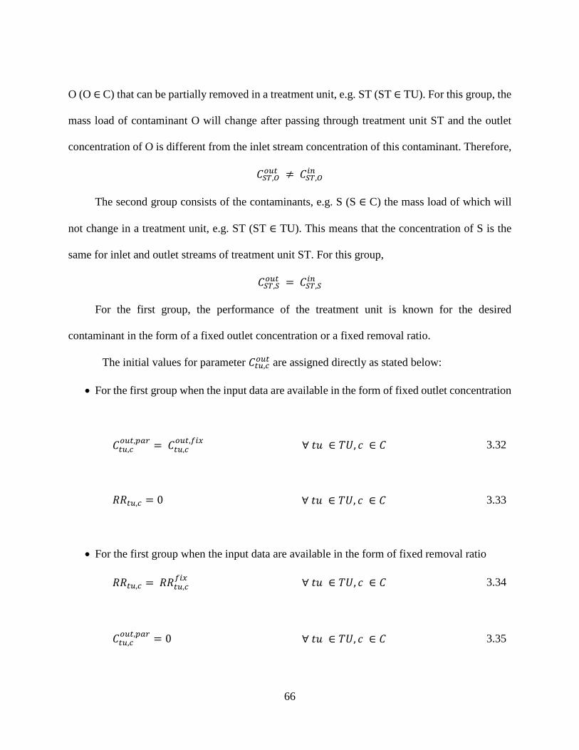
O (O ∈ C) that can be partially removed in a treatment unit, e.g. ST (ST ∈ TU). For this group, the
mass load of contaminant O will change after passing through treatment unit ST and the outlet
concentration of O is different from the inlet stream concentration of this contaminant. Therefore,
𝐶𝐶𝑆𝑆𝑇𝑇,𝑂𝑂𝑜𝑜𝑡𝑡𝑡𝑡 ≠ 𝐶𝐶𝑆𝑆𝑇𝑇,𝑂𝑂
𝑖𝑖𝑖𝑖
The second group consists of the contaminants, e.g. S (S ∈ C) the mass load of which will
not change in a treatment unit, e.g. ST (ST ∈ TU). This means that the concentration of S is the
same for inlet and outlet streams of treatment unit ST. For this group,
𝐶𝐶𝑆𝑆𝑇𝑇,𝑆𝑆𝑜𝑜𝑡𝑡𝑡𝑡 = 𝐶𝐶𝑆𝑆𝑇𝑇,𝑆𝑆
𝑖𝑖𝑖𝑖
For the first group, the performance of the treatment unit is known for the desired
contaminant in the form of a fixed outlet concentration or a fixed removal ratio.
The initial values for parameter 𝐶𝐶𝑡𝑡𝑡𝑡,𝑐𝑐𝑜𝑜𝑡𝑡𝑡𝑡 are assigned directly as stated below:
• For the first group when the input data are available in the form of fixed outlet concentration
𝐶𝐶𝑡𝑡𝑡𝑡,𝑐𝑐𝑜𝑜𝑡𝑡𝑡𝑡,𝑢𝑢𝑚𝑚𝑡𝑡 = 𝐶𝐶𝑡𝑡𝑡𝑡,𝑐𝑐
𝑜𝑜𝑡𝑡𝑡𝑡,𝑓𝑓𝑖𝑖𝑓𝑓 ∀ 𝑒𝑒𝑒𝑒 ∈ 𝑇𝑇𝑇𝑇, 𝑐𝑐 ∈ 𝐶𝐶 3.32
𝑅𝑅𝑅𝑅𝑡𝑡𝑡𝑡,𝑐𝑐 = 0 ∀ 𝑒𝑒𝑒𝑒 ∈ 𝑇𝑇𝑇𝑇, 𝑐𝑐 ∈ 𝐶𝐶 3.33
• For the first group when the input data are available in the form of fixed removal ratio
𝑅𝑅𝑅𝑅𝑡𝑡𝑡𝑡,𝑐𝑐 = 𝑅𝑅𝑅𝑅𝑡𝑡𝑡𝑡,𝑐𝑐𝑓𝑓𝑖𝑖𝑓𝑓 ∀ 𝑒𝑒𝑒𝑒 ∈ 𝑇𝑇𝑇𝑇, 𝑐𝑐 ∈ 𝐶𝐶 3.34
𝐶𝐶𝑡𝑡𝑡𝑡,𝑐𝑐𝑜𝑜𝑡𝑡𝑡𝑡,𝑢𝑢𝑚𝑚𝑡𝑡 = 0 ∀ 𝑒𝑒𝑒𝑒 ∈ 𝑇𝑇𝑇𝑇, 𝑐𝑐 ∈ 𝐶𝐶 3.35
66

• For the second group:
𝐶𝐶𝑡𝑡𝑡𝑡,𝑐𝑐𝑜𝑜𝑡𝑡𝑡𝑡,𝑢𝑢𝑚𝑚𝑡𝑡 = 0 ∀ 𝑒𝑒𝑒𝑒 ∈ 𝑇𝑇𝑇𝑇, 𝑐𝑐 ∈ 𝐶𝐶 3.36
𝑅𝑅𝑅𝑅𝑡𝑡𝑡𝑡,𝑐𝑐 = 0 ∀ 𝑒𝑒𝑒𝑒 ∈ 𝑇𝑇𝑇𝑇, 𝑐𝑐 ∈ 𝐶𝐶 3.37
A number of constraints are changed to a different form to simplify the optimization
procedure. New forms of equations 3.12 and 3.13, after projection onto concentration space, are
shown below:
��𝐹𝐹𝑡𝑡𝑡𝑡ʹ,𝑡𝑡𝑡𝑡 ∗ 𝐶𝐶𝑡𝑡𝑡𝑡,𝑐𝑐𝑜𝑜𝑡𝑡𝑡𝑡,𝑢𝑢𝑚𝑚𝑡𝑡 �
𝑡𝑡𝑡𝑡ʹ
+ ��𝐹𝐹𝑠𝑠,𝑡𝑡𝑡𝑡 ∗ 𝐶𝐶𝑠𝑠,𝑐𝑐�𝑠𝑠
− 𝑀𝑀𝑀𝑀𝑡𝑡𝑡𝑡,𝑐𝑐𝑖𝑖𝑖𝑖 = 0 ∀ 𝑒𝑒𝑒𝑒 ∈ 𝑇𝑇𝑇𝑇 , 𝑐𝑐 ∈ 𝐶𝐶 3.12ʹ
𝐶𝐶𝑡𝑡𝑡𝑡,𝑐𝑐𝑜𝑜𝑡𝑡𝑡𝑡,𝑢𝑢𝑚𝑚𝑡𝑡 ∗ ��𝐹𝐹𝑡𝑡𝑡𝑡ʹ,𝑡𝑡𝑡𝑡
𝑡𝑡𝑡𝑡ʹ
+ �𝐹𝐹𝑠𝑠,𝑡𝑡𝑡𝑡𝑠𝑠
− 𝐹𝐹𝑡𝑡𝑡𝑡𝑙𝑙𝑜𝑜𝑠𝑠𝑠𝑠� − 𝑀𝑀𝑀𝑀𝑡𝑡𝑡𝑡,𝑐𝑐𝑜𝑜𝑡𝑡𝑡𝑡 = 0 ∀ 𝑒𝑒𝑒𝑒 ∈ 𝑇𝑇𝑇𝑇, 𝑐𝑐 ∈ 𝐶𝐶 3.13ʹ
Constraint 3.15 is converted into an equality constraint and relaxed6 using slack and surplus
variables as:
��𝐹𝐹𝑡𝑡𝑡𝑡𝑒𝑒𝑓𝑓𝑖𝑖𝑡𝑡 ∗ 𝐶𝐶𝑡𝑡𝑡𝑡,𝑐𝑐𝑜𝑜𝑡𝑡𝑡𝑡,𝑢𝑢𝑚𝑚𝑡𝑡�
𝑡𝑡𝑡𝑡
+ 𝑐𝑐𝑐𝑐2 − 𝑐𝑐𝑐𝑐5 = 𝐶𝐶𝑐𝑐𝑡𝑡𝑚𝑚𝑡𝑡𝑡𝑡𝑒𝑒𝑡𝑡 ∗ �𝐹𝐹𝑡𝑡𝑡𝑡𝑒𝑒𝑓𝑓𝑖𝑖𝑡𝑡
𝑡𝑡𝑡𝑡
∀ 𝑐𝑐 ∈ 𝐶𝐶 3.15ʹ
6 Relaxation means adding an infeasibility term to the equation (𝑐𝑐𝑐𝑐5 in this equation) that helps keep the model feasible.
67

Variable 𝑐𝑐𝑐𝑐2 is used to change the inequality constraint to an equality and variable 𝑐𝑐𝑐𝑐5 is
used to relax the constraint and maintain feasibility. This variable is an infeasibility term and the
model attempts to reduce the term to zero during the optimization procedure.
Constraints 3.10 and 3.11 can be presented together in one equation. The relaxed form of
this constraint is shown as:
�1 − 𝑅𝑅𝑅𝑅𝑡𝑡𝑡𝑡,𝑐𝑐� ∗ 𝑀𝑀𝑀𝑀𝑡𝑡𝑡𝑡,𝑐𝑐𝑖𝑖𝑖𝑖 − 𝑀𝑀𝑀𝑀𝑡𝑡𝑡𝑡,𝑐𝑐
𝑜𝑜𝑡𝑡𝑡𝑡 − 𝑀𝑀𝑀𝑀𝑡𝑡𝑡𝑡,𝑐𝑐𝑡𝑡𝑒𝑒𝑚𝑚 − ∀ 𝑒𝑒𝑒𝑒 ∈ 𝑇𝑇𝑇𝑇 , 𝑐𝑐 ∈ 𝐶𝐶 3.10ʹ
𝐹𝐹𝑡𝑡𝑡𝑡𝑙𝑙𝑜𝑜𝑠𝑠𝑠𝑠 ∗ 𝐶𝐶𝑡𝑡𝑡𝑡𝑙𝑙𝑜𝑜𝑠𝑠𝑠𝑠 + 𝑀𝑀𝑀𝑀𝑡𝑡𝑡𝑡,𝑐𝑐𝑡𝑡𝑚𝑚𝑖𝑖𝑖𝑖 − 𝑀𝑀𝑀𝑀𝑡𝑡𝑡𝑡,𝑐𝑐
𝑙𝑙𝑜𝑜𝑠𝑠𝑠𝑠 = 0
𝑀𝑀𝑀𝑀𝑡𝑡𝑡𝑡,𝑐𝑐𝑡𝑡𝑚𝑚𝑖𝑖𝑖𝑖 and 𝑀𝑀𝑀𝑀𝑡𝑡𝑡𝑡,𝑐𝑐
𝑙𝑙𝑜𝑜𝑠𝑠𝑠𝑠 are slack and surplus variables that help maintain feasibility of the
problem and are considered as infeasibility terms which the procedure will aim to reduce to zero.
Equation 3.14 is converted to an equality constraint:
𝑀𝑀𝑀𝑀𝑡𝑡𝑡𝑡,𝑐𝑐𝑖𝑖𝑖𝑖 + 𝑐𝑐𝑡𝑡𝑡𝑡,𝑐𝑐
1 = 𝐶𝐶𝑡𝑡𝑡𝑡,𝑐𝑐𝑖𝑖𝑖𝑖,𝑚𝑚𝑚𝑚𝑓𝑓 ∗ 𝐹𝐹𝑡𝑡𝑡𝑡𝑖𝑖𝑖𝑖 ∀ 𝑒𝑒𝑒𝑒 ∈ 𝑇𝑇𝑇𝑇, 𝑐𝑐 ∈ 𝐶𝐶 3.14ʹ
Equation 3.16 is converted to an equality constraint and relaxed as:
�𝑀𝑀𝑀𝑀𝑡𝑡𝑡𝑡,𝑐𝑐𝑡𝑡𝑒𝑒𝑚𝑚
𝑡𝑡𝑡𝑡
+ ��𝑅𝑅𝑅𝑅𝑡𝑡𝑡𝑡,𝑐𝑐 ∗ 𝑀𝑀𝑀𝑀𝑡𝑡𝑡𝑡,𝑐𝑐𝑖𝑖𝑖𝑖 �
𝑡𝑡𝑡𝑡
∀ 𝑐𝑐 ∈ 𝐶𝐶 3.16ʹ
− 𝑐𝑐𝑐𝑐4 + 𝑐𝑐𝑐𝑐3 = 𝑀𝑀𝑀𝑀𝑐𝑐𝑡𝑡𝑒𝑒𝑚𝑚
68
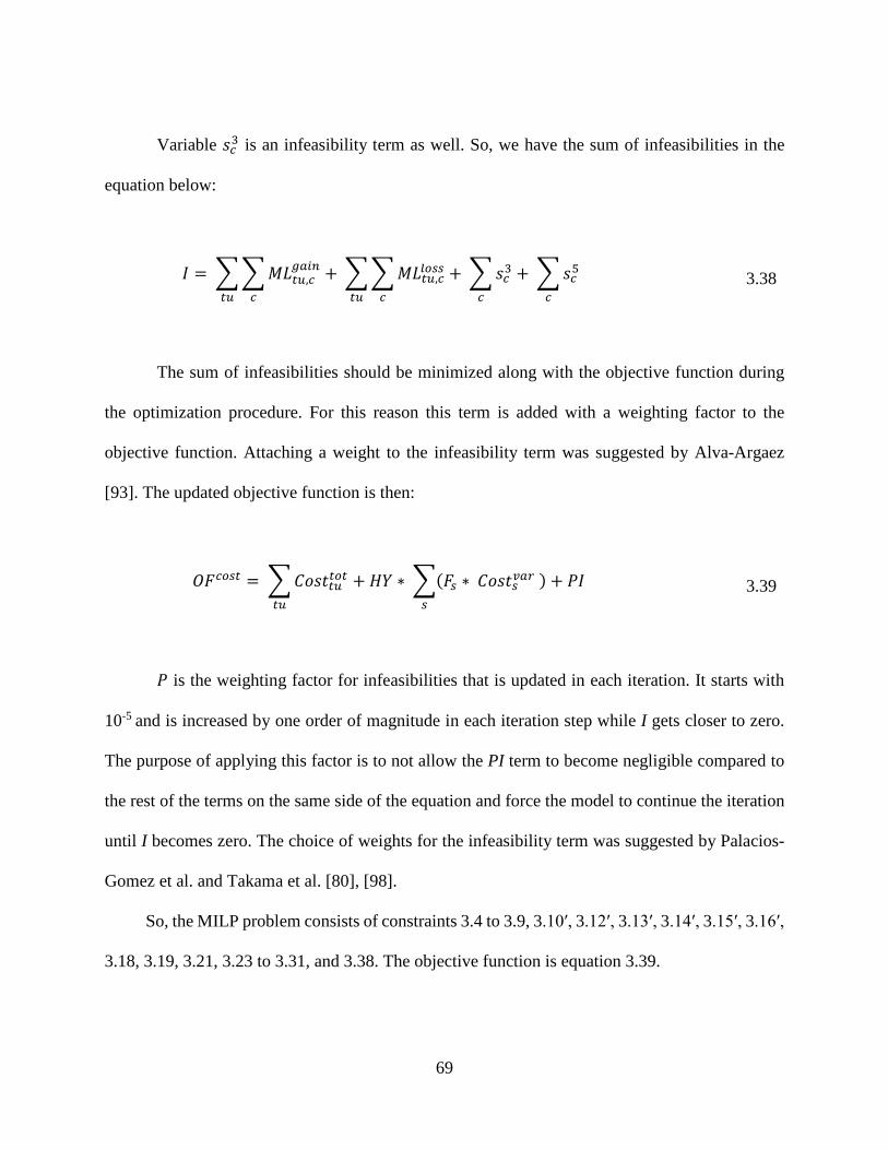
Variable 𝑐𝑐𝑐𝑐3 is an infeasibility term as well. So, we have the sum of infeasibilities in the
equation below:
𝐼𝐼 = ��𝑀𝑀𝑀𝑀𝑡𝑡𝑡𝑡,𝑐𝑐𝑡𝑡𝑚𝑚𝑖𝑖𝑖𝑖
𝑐𝑐𝑡𝑡𝑡𝑡
+ ��𝑀𝑀𝑀𝑀𝑡𝑡𝑡𝑡,𝑐𝑐𝑙𝑙𝑜𝑜𝑠𝑠𝑠𝑠
𝑐𝑐𝑡𝑡𝑡𝑡
+ �𝑐𝑐𝑐𝑐3𝑐𝑐
+ �𝑐𝑐𝑐𝑐5𝑐𝑐
3.38
The sum of infeasibilities should be minimized along with the objective function during
the optimization procedure. For this reason this term is added with a weighting factor to the
objective function. Attaching a weight to the infeasibility term was suggested by Alva-Argaez
[93]. The updated objective function is then:
𝑂𝑂𝐹𝐹𝑐𝑐𝑜𝑜𝑠𝑠𝑡𝑡 = �𝐶𝐶𝑐𝑐𝑐𝑐𝑒𝑒𝑡𝑡𝑡𝑡𝑡𝑡𝑜𝑜𝑡𝑡𝑡𝑡𝑡𝑡
+ 𝐻𝐻𝐻𝐻 ∗ �(𝐹𝐹𝑠𝑠 ∗ 𝐶𝐶𝑐𝑐𝑐𝑐𝑒𝑒𝑠𝑠𝑎𝑎𝑚𝑚𝑡𝑡 )𝑠𝑠
+ 𝑃𝑃𝐼𝐼 3.39
𝑃𝑃 is the weighting factor for infeasibilities that is updated in each iteration. It starts with
10-5 and is increased by one order of magnitude in each iteration step while I gets closer to zero.
The purpose of applying this factor is to not allow the PI term to become negligible compared to
the rest of the terms on the same side of the equation and force the model to continue the iteration
until I becomes zero. The choice of weights for the infeasibility term was suggested by Palacios-
Gomez et al. and Takama et al. [80], [98].
So, the MILP problem consists of constraints 3.4 to 3.9, 3.10ʹ, 3.12ʹ, 3.13ʹ, 3.14ʹ, 3.15ʹ, 3.16ʹ,
3.18, 3.19, 3.21, 3.23 to 3.31, and 3.38. The objective function is equation 3.39.
69

3.5.2 The linear programming (LP) problem
The constraints of the LP problem include equation 3.10ʹ, and equations 3.12 and 3.13
projected onto the 𝐹𝐹𝑡𝑡𝑡𝑡ʹ,𝑡𝑡𝑡𝑡 and 𝐹𝐹𝑠𝑠,𝑡𝑡𝑡𝑡 space. Initial values for 𝐹𝐹𝑡𝑡𝑡𝑡ʹ,𝑡𝑡𝑡𝑡 and 𝐹𝐹𝑠𝑠,𝑡𝑡𝑡𝑡 are available from the
results of the MILP problem. Using the new constraints, the outlet concentration, 𝐶𝐶𝑡𝑡𝑡𝑡,𝑐𝑐𝑜𝑜𝑡𝑡𝑡𝑡 is an
unknown variable and stream flow rates, 𝐹𝐹𝑡𝑡𝑡𝑡ʹ,𝑡𝑡𝑡𝑡 and 𝐹𝐹𝑠𝑠,𝑡𝑡𝑡𝑡 from equations 3.12 and 3.13 are assumed
to be known parameters and are written in the form of 𝐹𝐹𝑡𝑡𝑡𝑡ʹ,𝑡𝑡𝑡𝑡𝑢𝑢𝑚𝑚𝑡𝑡 and 𝐹𝐹𝑠𝑠,𝑡𝑡𝑡𝑡
𝑢𝑢𝑚𝑚𝑡𝑡 respectively.
��𝐹𝐹𝑡𝑡𝑡𝑡ʹ,𝑡𝑡𝑡𝑡𝑢𝑢𝑚𝑚𝑡𝑡 ∗ 𝐶𝐶𝑡𝑡𝑡𝑡,𝑐𝑐
𝑜𝑜𝑡𝑡𝑡𝑡 �𝑡𝑡𝑡𝑡ʹ
+ ��𝐹𝐹𝑠𝑠,𝑡𝑡𝑡𝑡𝑢𝑢𝑚𝑚𝑡𝑡 ∗ 𝐶𝐶𝑠𝑠,𝑐𝑐�
𝑠𝑠
− 𝑀𝑀𝑀𝑀𝑡𝑡𝑡𝑡,𝑐𝑐𝑖𝑖𝑖𝑖 = 0 ∀ 𝑒𝑒𝑒𝑒 ∈ 𝑇𝑇𝑇𝑇 , 𝑐𝑐 ∈ 𝐶𝐶 3.12ʹʹ
𝐶𝐶𝑡𝑡𝑡𝑡,𝑐𝑐𝑜𝑜𝑡𝑡𝑡𝑡 ∗ ��𝐹𝐹𝑡𝑡𝑡𝑡ʹ,𝑡𝑡𝑡𝑡
𝑢𝑢𝑚𝑚𝑡𝑡
𝑡𝑡𝑡𝑡ʹ
+ �𝐹𝐹𝑠𝑠,𝑡𝑡𝑡𝑡𝑢𝑢𝑚𝑚𝑡𝑡
𝑠𝑠
− 𝐹𝐹𝑡𝑡𝑡𝑡𝑙𝑙𝑜𝑜𝑠𝑠𝑠𝑠� − 𝑀𝑀𝑀𝑀𝑡𝑡𝑡𝑡,𝑐𝑐𝑜𝑜𝑡𝑡𝑡𝑡 = 0 ∀ 𝑒𝑒𝑒𝑒 ∈ 𝑇𝑇𝑇𝑇, 𝑐𝑐 ∈ 𝐶𝐶 3.13ʹʹ
In the LP problem the goal is to minimize the sum of infeasibilities that appear in the
problem constraints. The objective function of the LP problem is named M and is in the form of:
𝑀𝑀 = ��𝑀𝑀𝑀𝑀𝑡𝑡𝑡𝑡,𝑐𝑐𝑡𝑡𝑚𝑚𝑖𝑖𝑖𝑖
𝑐𝑐𝑡𝑡𝑡𝑡
+ ��𝑀𝑀𝑀𝑀𝑡𝑡𝑡𝑡,𝑐𝑐𝑙𝑙𝑜𝑜𝑠𝑠𝑠𝑠
𝑐𝑐𝑡𝑡𝑡𝑡
∀ 𝑒𝑒𝑒𝑒 ∈ 𝑇𝑇𝑇𝑇, 𝑐𝑐 ∈ 𝐶𝐶 3.40
Let MILPk and LPk be the mixed-integer linear problem and the linear problem at iteration
k. The approach to solve this, is described in the following steps:
1. Set k=1. Outlet contaminants concentration and removal ratios are initialized as described in
equations 3.32 to 3.37 for the first iteration.
70

2. The MILPk is solved to minimize the objective function and optimal values of flow rates are
found: 𝐹𝐹𝑠𝑠,𝑡𝑡𝑡𝑡∗, 𝐹𝐹𝑡𝑡𝑡𝑡,𝑡𝑡𝑡𝑡ˊ
∗, 𝐹𝐹𝑡𝑡𝑡𝑡𝑒𝑒𝑓𝑓𝑖𝑖𝑡𝑡∗, 𝐹𝐹𝑡𝑡𝑡𝑡𝑖𝑖𝑖𝑖
∗, 𝐹𝐹𝑡𝑡𝑡𝑡𝑜𝑜𝑡𝑡𝑡𝑡∗.
3. Set 𝐹𝐹𝑠𝑠,𝑡𝑡𝑡𝑡𝑢𝑢𝑚𝑚𝑡𝑡,𝑘𝑘 = 𝐹𝐹𝑠𝑠,𝑡𝑡𝑡𝑡
∗ and 𝐹𝐹𝑡𝑡𝑡𝑡ʹ,𝑡𝑡𝑡𝑡𝑢𝑢𝑚𝑚𝑡𝑡,𝑘𝑘 = 𝐹𝐹𝑡𝑡𝑡𝑡,𝑡𝑡𝑡𝑡ˊ
∗ and solve the LPk to find a new outlet
concentration vector 𝐶𝐶𝑡𝑡𝑡𝑡,𝑐𝑐𝑜𝑜𝑡𝑡𝑡𝑡∗.
4. Increase the iteration number by one unit: k=k+1. Set 𝑃𝑃𝑘𝑘+1 = 𝑃𝑃𝑘𝑘 ∗ 10 and 𝐶𝐶𝑡𝑡𝑡𝑡,𝑐𝑐𝑜𝑜𝑡𝑡𝑡𝑡,𝑘𝑘+1 =
𝐶𝐶𝑡𝑡𝑡𝑡,𝑐𝑐𝑜𝑜𝑡𝑡𝑡𝑡∗. Then solve the MILPk to find new values for the stream flow rates.
5. If 𝐼𝐼 ≤ 𝜀𝜀 stop. Otherwise repeat the procedure from step 3.
This procedure iterates between the two problems (MILP and LP) until the sum of
infeasibilities is close to zero (𝜀𝜀 = 10−5). The optimal values of the objective function and flow
rates from the last iteration when feasibility is reached can then be used as the initial point for the
MINLP problem. In most cases the results of the last iteration are similar to the results of the
MINLP problem, but in some case the MINLP problem improves (gives a smaller value for the
objective function) the results of the iteration.
In this procedure a penalty term (sum of infeasibilities) is added to the objective function
of the MINLP problem to account for the infeasibilities that are imposed on the model by the initial
assumption of perfect treatment performance. This assumption is essential to remove the nonlinear
terms and converts the feasible region of the problem to a convex set. The iterative approach helps
decrease the infeasibility term step by step until it converges to zero.
CPLEX solver is used for the linear models and BARON is used for the nonlinear models
in the study. CPLEX is a high performance solver for LP and MIP problems and is the most widely
used commercial MIP solver. This solver uses the primal or dual simplex algorithm, the barrier
algorithm or the network algorithm to solve the problems [99]. The Branch-And-Reduce
71
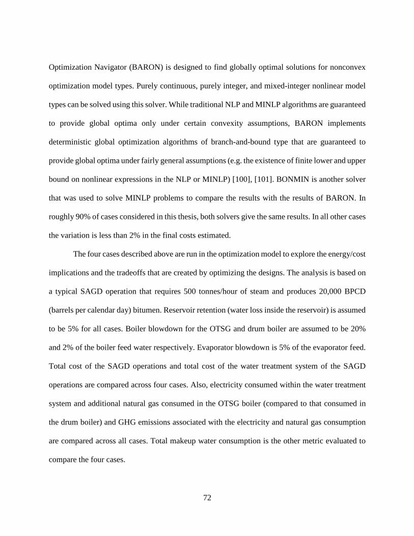
Optimization Navigator (BARON) is designed to find globally optimal solutions for nonconvex
optimization model types. Purely continuous, purely integer, and mixed-integer nonlinear model
types can be solved using this solver. While traditional NLP and MINLP algorithms are guaranteed
to provide global optima only under certain convexity assumptions, BARON implements
deterministic global optimization algorithms of branch-and-bound type that are guaranteed to
provide global optima under fairly general assumptions (e.g. the existence of finite lower and upper
bound on nonlinear expressions in the NLP or MINLP) [100], [101]. BONMIN is another solver
that was used to solve MINLP problems to compare the results with the results of BARON. In
roughly 90% of cases considered in this thesis, both solvers give the same results. In all other cases
the variation is less than 2% in the final costs estimated.
The four cases described above are run in the optimization model to explore the energy/cost
implications and the tradeoffs that are created by optimizing the designs. The analysis is based on
a typical SAGD operation that requires 500 tonnes/hour of steam and produces 20,000 BPCD
(barrels per calendar day) bitumen. Reservoir retention (water loss inside the reservoir) is assumed
to be 5% for all cases. Boiler blowdown for the OTSG and drum boiler are assumed to be 20%
and 2% of the boiler feed water respectively. Evaporator blowdown is 5% of the evaporator feed.
Total cost of the SAGD operations and total cost of the water treatment system of the SAGD
operations are compared across four cases. Also, electricity consumed within the water treatment
system and additional natural gas consumed in the OTSG boiler (compared to that consumed in
the drum boiler) and GHG emissions associated with the electricity and natural gas consumption
are compared across all cases. Total makeup water consumption is the other metric evaluated to
compare the four cases.
72

Chapter Four: Results and Discussion
The optimization of the water treatment network of SAGD operations for four different
configuration scenarios (case 1 to case 4) is explored and presented in this chapter. For each case,
the current and optimized designs are compared across a set of metrics (cost, energy, GHG
emissions, etc.). Additionally, four cases are compared to each other in order to explore
cost/energy/water/GHG emissions tradeoffs within and across different cases. The analysis is
based on a typical SAGD operation that requires 500 tonnes/hour of steam and produces 20,000
BPCD (barrels per calendar day) bitumen.
4.1 Optimized design for minimum total cost
The optimized designs resulting from the optimization of 4 cases for minimized cost (i.e.
by deploying the cost objective function) are presented here. Figure 4-1 to Figure 4-4 show the
current designs for the SAGD water treatment network for four cases. Optimized designs for case
1 to 4 are shown in Figure 4-5 to Figure 4-8.
73

Figure 4-1 Current design of water treatment network for case 1 (all stream flow rates are in
tonne/hr)
Figure 4-2 Current design of water treatment network for case 2 (all stream flow rates are in
tonne/hr)
74
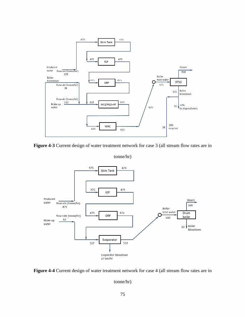
Figure 4-3 Current design of water treatment network for case 3 (all stream flow rates are in
tonne/hr)
Figure 4-4 Current design of water treatment network for case 4 (all stream flow rates are in
tonne/hr)
75
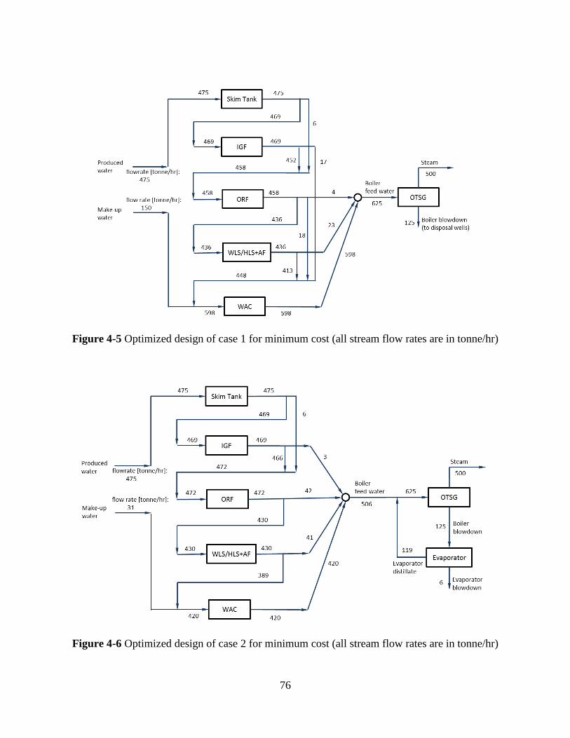
Figure 4-5 Optimized design of case 1 for minimum cost (all stream flow rates are in tonne/hr)
Figure 4-6 Optimized design of case 2 for minimum cost (all stream flow rates are in tonne/hr)
76
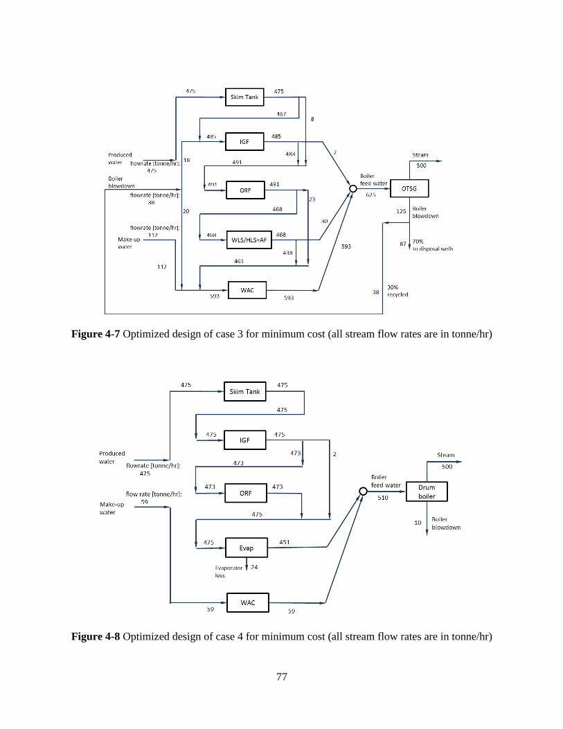
Figure 4-7 Optimized design of case 3 for minimum cost (all stream flow rates are in tonne/hr)
Figure 4-8 Optimized design of case 4 for minimum cost (all stream flow rates are in tonne/hr)
77
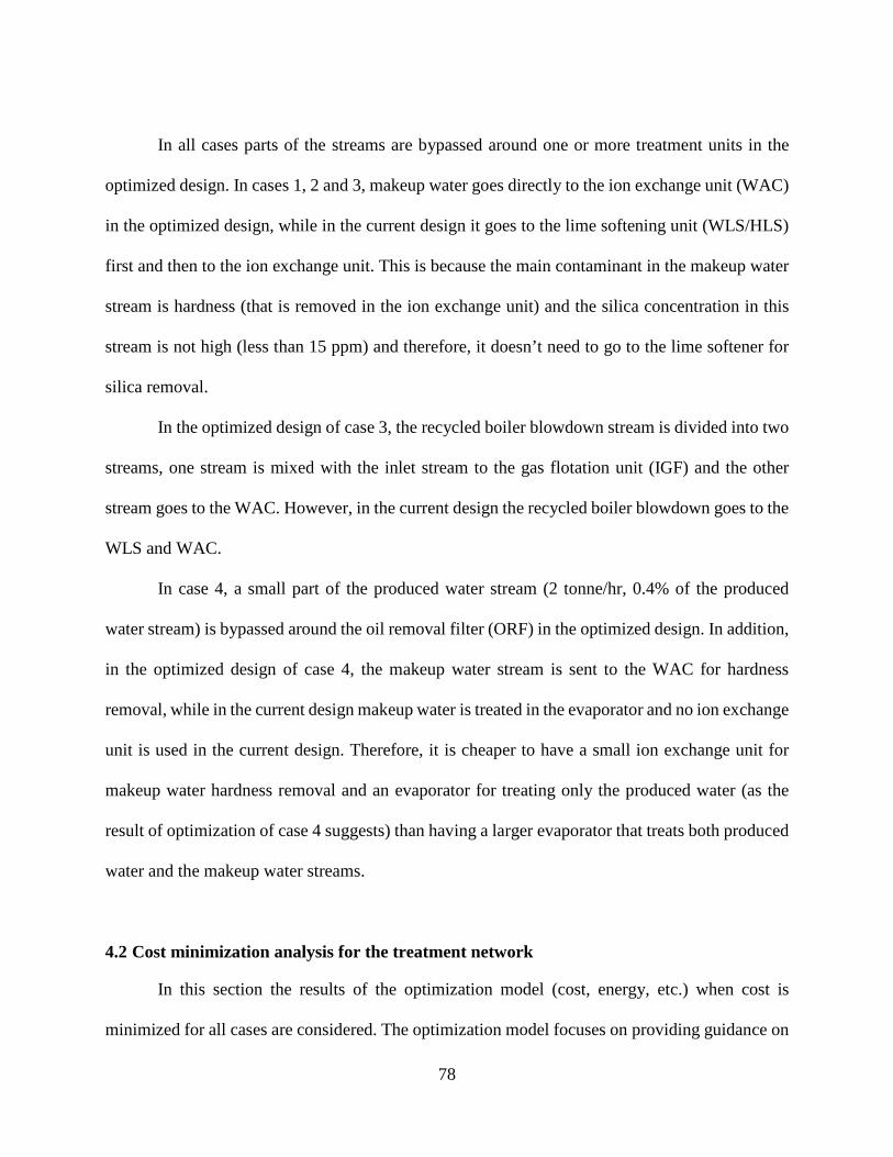
In all cases parts of the streams are bypassed around one or more treatment units in the
optimized design. In cases 1, 2 and 3, makeup water goes directly to the ion exchange unit (WAC)
in the optimized design, while in the current design it goes to the lime softening unit (WLS/HLS)
first and then to the ion exchange unit. This is because the main contaminant in the makeup water
stream is hardness (that is removed in the ion exchange unit) and the silica concentration in this
stream is not high (less than 15 ppm) and therefore, it doesn’t need to go to the lime softener for
silica removal.
In the optimized design of case 3, the recycled boiler blowdown stream is divided into two
streams, one stream is mixed with the inlet stream to the gas flotation unit (IGF) and the other
stream goes to the WAC. However, in the current design the recycled boiler blowdown goes to the
WLS and WAC.
In case 4, a small part of the produced water stream (2 tonne/hr, 0.4% of the produced
water stream) is bypassed around the oil removal filter (ORF) in the optimized design. In addition,
in the optimized design of case 4, the makeup water stream is sent to the WAC for hardness
removal, while in the current design makeup water is treated in the evaporator and no ion exchange
unit is used in the current design. Therefore, it is cheaper to have a small ion exchange unit for
makeup water hardness removal and an evaporator for treating only the produced water (as the
result of optimization of case 4 suggests) than having a larger evaporator that treats both produced
water and the makeup water streams.
4.2 Cost minimization analysis for the treatment network
In this section the results of the optimization model (cost, energy, etc.) when cost is
minimized for all cases are considered. The optimization model focuses on providing guidance on
78

decisions related to the water treatment system. Therefore, results include comparisons of different
water treatment technologies and the remainder of the SAGD operation (e.g., steam generation
and waste disposal) is not presented. Of specific note, the impact of the difference in the boiler
costs (difference between OTSG and drum boiler costs) and the difference in natural gas
combustion in different types of boiler (OTSG and drum boiler) are considered in results presented
in this chapter, not the entire steam production section (i.e. the results get dwarfed since the cost
of the water treatment system is about 12.5-25% of the total cost of the plant for different
configurations. We acknowledge that the emissions and costs are relatively small when compared
to the total plant, however, they are still on the order of millions of dollars per year and therefore
are important to investigate.). However, the results in the context of the entire facility are presented
in Appendix A.
4.2.1 Operating cost breakdown
The total cost of the water treatment system for current and optimized designs for the four
cases are shown in Figure 4-9. In this figure, the operating cost of the water treatment system
(WTS) is divided into the electricity cost, chemicals cost and other costs (e.g. maintenance cost,
manpower cost, etc.).
79

Figure 4-9 Annual cost of the water treatment system for cases 1-4, with operating cost
breakdown
For each case, costs of the current and optimized designs are shown in Figure 4-9.
According to this figure, the cost of the water treatment system decreases due to the improvements
that are recommended through the optimization model (that are shown in Figure 4-1 to Figure 4-
8). In the optimized design of all the four cases, stream flow rates passing all or some of the
treatment units are reduced. Smaller flow rate results in smaller treatment units, which means
lower cost of treatment unit. Cases 1 and 3 show the highest potential for cost savings with 19.5%
and 15.8% cost savings respectively. Cases 2 and 4 show the lowest with 7% and 9% potential
cost savings. However, all optimized cases result in lower costs than the corresponding “current”
02468
10121416182022242628
Case 1 Case 2 Case 3 Case 4
Annu
al c
ost (
$1E6
/yr)
Chemicals CostNatural Gas CostElectricity CostOther CostsCapital Cost
Operating Cost:
80

cases. The contribution of operating cost to the total cost savings is about 15-30% higher than the
contribution of capital cost for all cases. This means that operating cost has a more significant
share of the potential savings than capital cost especially in the treatment units making larger
contributions to the cost savings.
Electricity represents a small share of the total operating cost in cases 1 and 3 (16% and
14% respectively). In cases 2 and 4 where the evaporator is used for water treatment, the share of
electricity in total operating cost is more significant (36% and 63% respectively). Optimizing the
flow of the streams also leads to savings in electricity. These savings are relatively small for cases
1, 2 and 3 (from 5.8% to 6.3% of the total operating cost savings) but are more significant for case
4 (60% of total operating cost savings). This is due to the use of evaporators in case 4. That is,
more than 95% of total electricity consumption of case 4, is used in the evaporator and this case
consumes 3.5-13 times more electricity than cases 1, 2 and 3. Therefore, bypassing wastewater
streams around the evaporator where possible will result in a reduction in the electricity used in
case 4 more than other components of the operating cost.
The results also show that case 1 has the lowest cost of water treatment system and cases
3, 2 and 4 rank next respectively. The higher cost of cases 2 and 4 is due to the use of evaporators
that are more expensive than other treatment units. All the detailed cost results are presented in
Appendix B, Table B-1 to Table B-4.
To include the impact of the steam generation component of the water treatment system,
the total cost of the water treatment system plus the additional capital and operating cost associated
with the steam generation system, for current and optimized designs for the four cases are shown
in Figure 4-10 (total capital cost of drum boiler used in case 4 is higher than OTSG used in cases
1, 2 and 3, while total operating cost of OTSG is higher than drum boiler). Only the cost differences
81
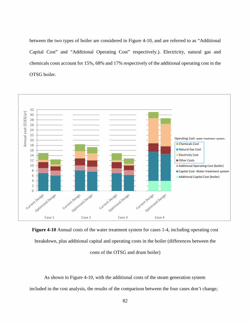
between the two types of boiler are considered in Figure 4-10, and are referred to as “Additional
Capital Cost” and “Additional Operating Cost” respectively.). Electricity, natural gas and
chemicals costs account for 15%, 68% and 17% respectively of the additional operating cost in the
OTSG boiler.
Figure 4-10 Annual costs of the water treatment system for cases 1-4, including operating cost
breakdown, plus additional capital and operating costs in the boiler (differences between the
costs of the OTSG and drum boiler)
As shown in Figure 4-10, with the additional costs of the steam generation system
included in the cost analysis, the results of the comparison between the four cases don’t change;
02468
101214161820222426283032
Case 1 Case 2 Case 3 Case 4
Annu
al c
ost (
$1E6
/yr)
Chemicals Cost
Natural Gas Cost
Electricity Cost
Other Costs
Additional Operating Cost (boiler)
Capital Cost- Water treatment system
Additional Capital Cost (boiler)
Operating Cost- water treatmenr system:
82

case 4 is still the most expensive case and cases 2, 3 and 1 are increasingly less costly. This
means the additional costs for the steam generation system are not significant in the cost analysis
of the four cases and therefore are not included in the results presented in the remaining of the
chapter.
Capital and operating cost breakdown by treatment unit
Figure 4-11 shows the total cost of the water treatment system including capital and
operating cost broken down by treatment unit.
Figure 4-11 Annual cost of the water treatment system for cases 1-4, with capital and operating
cost broken down by treatment unit (CC=Capital cost- solid fill, OC=Operating cost- hashed fill)
0
2
4
6
8
10
12
14
16
18
20
22
24
26
28
Case 1 Case 2 Case 3 Case 4
Annu
al c
ost (
$1E6
/yr)
Makeup Water
Evaporator
WAC
WLS
ORF
IGF
Skim Tank
CC
OC
83

According to Figure 4-11, in cases 1 and 3 the lime softener contributes the largest share
of both capital and operating cost. In case 2, the lime softener and evaporator constitute more than
90% of the total operating cost and about 50% of the total capital cost. In case 4, the evaporator is
the major contributor to the total capital (about 70%) and operating cost (more than 90%) of the
water treatment system.
Cost savings associated with each treatment unit are also investigated here. The results
show that in cases 1 to 3 the lime softener accounts for more than 90% of both capital and operating
cost savings in the water treatment system. In case 4, the evaporator accounts for almost all the
savings in the capital and operating cost. This suggests that to minimize cost via process
modifications, it is better to start by improving the lime softening unit and the evaporator efficiency
rather than other treatment units. Detailed cost results for treatment units are shown in Appendix
B, Table B-5 to Table B-8.
In some cases negative values are reported for the cost savings in a treatment unit, e.g. ion
exchange in case 4 (Appendix B, Table B-8). This is due to the use of treatment units in the
optimized design that are not used in the current design. In other words, when a unit is not part of
the current treatment system design like the ion exchange unit in case 4, the cost of that unit is zero
in the current design. Then, if that unit is selected in the optimized design, it will result in a negative
value for savings for that specific unit (i.e., a cost). In case 4 the ion exchange unit is part of the
optimized design, because the use of the ion exchange unit can reduce the contaminant load on the
evaporator and therefore reduce its size. This consequently leads to a lower total cost.
According to the results of the cost analysis for the entire plant (presented in Appendix A),
the total cost of the whole SAGD process (water treatment, steam generation, steam injection,
waste disposal, etc.) is estimated to be between $11.9 and $14.4 per barrel of bitumen produced.
84
4.2.2 Energy consumption analysis
The energy consumption associated with cases 1 through 4 are presented here. It should be
noted that these are the same cases presented above (i.e., the optimization model is run using the
cost minimization objective function). Later in this chapter, the impacts of running the
optimization model to minimize energy consumption are explored.
Figure 4-12 shows the electricity consumption7 in the water treatment system for the four
cases in the current and optimized design broken down by treatment unit.
7 In SAGD operations, NG is used for steam generation in the boilers and is not used directly in the water treatment system. Electricity is therefore the only form of energy that is used in the treatment system and this can be generated using natural gas or purchased from the Alberta electricity grid.
85
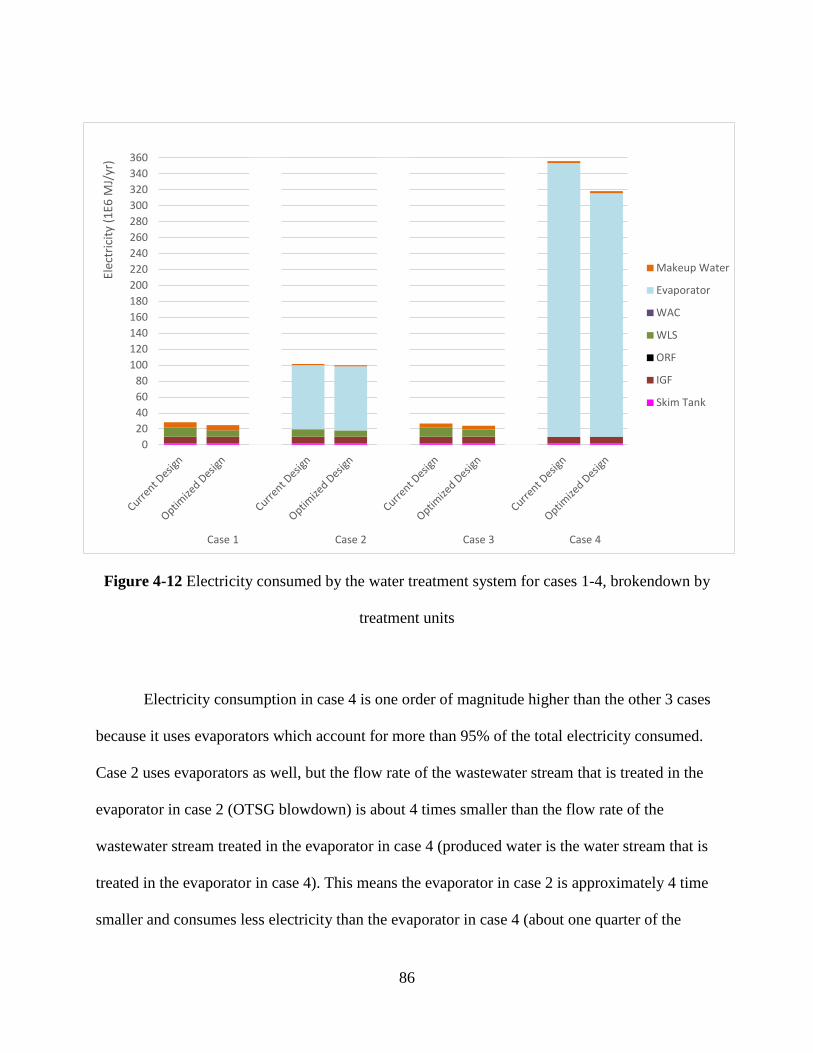
Figure 4-12 Electricity consumed by the water treatment system for cases 1-4, brokendown by
treatment units
Electricity consumption in case 4 is one order of magnitude higher than the other 3 cases
because it uses evaporators which account for more than 95% of the total electricity consumed.
Case 2 uses evaporators as well, but the flow rate of the wastewater stream that is treated in the
evaporator in case 2 (OTSG blowdown) is about 4 times smaller than the flow rate of the
wastewater stream treated in the evaporator in case 4 (produced water is the water stream that is
treated in the evaporator in case 4). This means the evaporator in case 2 is approximately 4 time
smaller and consumes less electricity than the evaporator in case 4 (about one quarter of the
020406080
100120140160180200220240260280300320340360
Case 1 Case 2 Case 3 Case 4
Elec
tric
ity (1
E6 M
J/yr
)
Makeup Water
Evaporator
WAC
WLS
ORF
IGF
Skim Tank
86
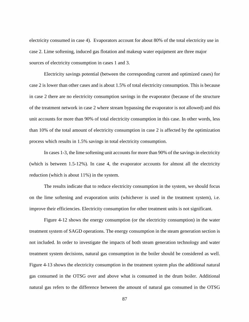
electricity consumed in case 4). Evaporators account for about 80% of the total electricity use in
case 2. Lime softening, induced gas flotation and makeup water equipment are three major
sources of electricity consumption in cases 1 and 3.
Electricity savings potential (between the corresponding current and optimized cases) for
case 2 is lower than other cases and is about 1.5% of total electricity consumption. This is because
in case 2 there are no electricity consumption savings in the evaporator (because of the structure
of the treatment network in case 2 where stream bypassing the evaporator is not allowed) and this
unit accounts for more than 90% of total electricity consumption in this case. In other words, less
than 10% of the total amount of electricity consumption in case 2 is affected by the optimization
process which results in 1.5% savings in total electricity consumption.
In cases 1-3, the lime softening unit accounts for more than 90% of the savings in electricity
(which is between 1.5-12%). In case 4, the evaporator accounts for almost all the electricity
reduction (which is about 11%) in the system.
The results indicate that to reduce electricity consumption in the system, we should focus
on the lime softening and evaporation units (whichever is used in the treatment system), i.e.
improve their efficiencies. Electricity consumption for other treatment units is not significant.
Figure 4-12 shows the energy consumption (or the electricity consumption) in the water
treatment system of SAGD operations. The energy consumption in the steam generation section is
not included. In order to investigate the impacts of both steam generation technology and water
treatment system decisions, natural gas consumption in the boiler should be considered as well.
Figure 4-13 shows the electricity consumption in the treatment system plus the additional natural
gas consumed in the OTSG over and above what is consumed in the drum boiler. Additional
natural gas refers to the difference between the amount of natural gas consumed in the OTSG
87

(cases 1, 2 and 3) and the natural gas consumed in the drum boiler (case 4). The amount of natural
gas consumed per cubic meter of boiler feed water is a little higher for drum boilers than that for
OTSGs (based on the data we have). However, because for the same amount of required steam,
the drum boiler needs less boiler feed water (the drum boiler generates only 1-2% blowdown from
the boiler feed water while the OTSG generates about 20% blowdown), total natural gas
consumption for cases 1-3 that use OTSG is higher that case 4 that uses drum boiler. The reason
for presenting the difference between natural gas consumption in the two types of boiler instead
of presenting the total amount of natural gas consumption for each type of boiler is to show the
differences between the energy consumption in four cases in a more visually distinguishable
manner. It should be noted that since the optimization doesn’t affect the steam generation section
of the plant, natural gas consumed in the current and optimized designs of each case are equal.
Therefore, only the results of the optimized designs are shown in Figure 4-13.
88
Figure 4-13 Energy consumption SAGD operations for cases 1-4 (electricity consumed in water
treatment system and additional natural gas consumption in the OTSG above what is consumed
in the drum boiler)
Cases 1-3 all consume more natural gas than Case 4 because they all employ an OTSG.
However, when the total energy consumed is included (both additional natural gas and electricity),
the results of energy consumption are similar (only a 20% difference between the lowest and
highest energy consumption (cases 1 and 2) compared to the 92% difference between the lowest
and highest electricity consumption (cases 1 and 4) in Figure 4-12). However, Case 2 has the
highest total energy consumption among all four cases. Since the type of energy is different for
020406080
100120140160180200220240260280300320340360380
Optimized DesignCase 1
Optimized DesignCase 2
Optimized DesignCase 3
Optimized DesignCase 4
Ener
gy C
onsu
mpt
ion
(1E6
MJ/
yr)
Additonal NG
Electricity
89
each case, the environmental implications of the different systems will be quite different. Detailed
results of energy consumption are presented in Appendix A, Table A-5 and Appendix B, Table B-
9 to Table B-12.
4.2.3 GHG emissions analysis
GHG emissions associated with the water treatment system (that come from the electricity
consumption in the water treatment system) are proportionally related to the electricity
consumption shown in Figure 4-12. GHG emissions from electricity are much higher for case 4
(3.5-13 time higher than cases 1, 2 and 3) due to the significant consumption of electricity in the
evaporator (8.5E07 kWh/year). However, if we also include the emissions associated with the
natural gas burned to compensate for the increased energy requirements of the OTSG (compared
with the drum boiler), the GHG emissions difference between cases narrows somewhat (for
example case 4 has 1.8-3.2 more GHG emissions than cases 1, 2 and 3 rather than 3.5-13 more
GHG emissions if only electricity is considered). GHG emissions from electricity and additional
natural gas consumption in the OTSG are shown in Figure 4-14.
90

Figure 4-14 GHG emissions from electricity and use of additional natural gas in the OTSG
According to Figure 4-14, case 4 still has the largest GHG emissions, even though the total
energy consumed in case 4 is lower than case 2 (energy consumption of cases 2 and 4 are 3.8E08
MJ/year and 3.2E08 MJ/year respectively. GHG emissions of case 2 and 4 are 3.6E04 tCO2/year
and 6.5E04 tCO2/year respectively). The reason is that natural gas has a lower GHG intensity (per
MJ) than electricity (the electricity emissions factor assumed in this analysis for Alberta’s
electricity grid is 0.75 tCO2 per MWh [102]), and since the majority of the energy used in case 2
is natural gas, total GHG emissions in this case is lower than case 4. The electricity emissions
factor is an important factor in determining the relative GHG emissions of cases 2 and 4. However,
the emissions intensity of electricity from Alberta grid varies greatly from year to year. It would
take a low carbon source of electricity (e.g., from renewable or nuclear), for the total emissions of
0
5
10
15
20
25
30
35
40
45
50
55
60
65
Optimized DesignCase 1
Optimized DesignCase 2
Optimized DesignCase 3
Optimized DesignCase 4
GHG
Emiss
ions
(1E3
tCO
2/yr
)
GHG emissions-Additional NG
GHG emissions-Electricity
91
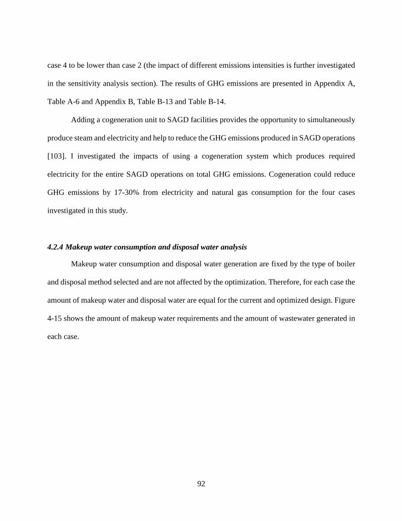
case 4 to be lower than case 2 (the impact of different emissions intensities is further investigated
in the sensitivity analysis section). The results of GHG emissions are presented in Appendix A,
Table A-6 and Appendix B, Table B-13 and Table B-14.
Adding a cogeneration unit to SAGD facilities provides the opportunity to simultaneously
produce steam and electricity and help to reduce the GHG emissions produced in SAGD operations
[103]. I investigated the impacts of using a cogeneration system which produces required
electricity for the entire SAGD operations on total GHG emissions. Cogeneration could reduce
GHG emissions by 17-30% from electricity and natural gas consumption for the four cases
investigated in this study.
4.2.4 Makeup water consumption and disposal water analysis
Makeup water consumption and disposal water generation are fixed by the type of boiler
and disposal method selected and are not affected by the optimization. Therefore, for each case the
amount of makeup water and disposal water are equal for the current and optimized design. Figure
4-15 shows the amount of makeup water requirements and the amount of wastewater generated in
each case.
92
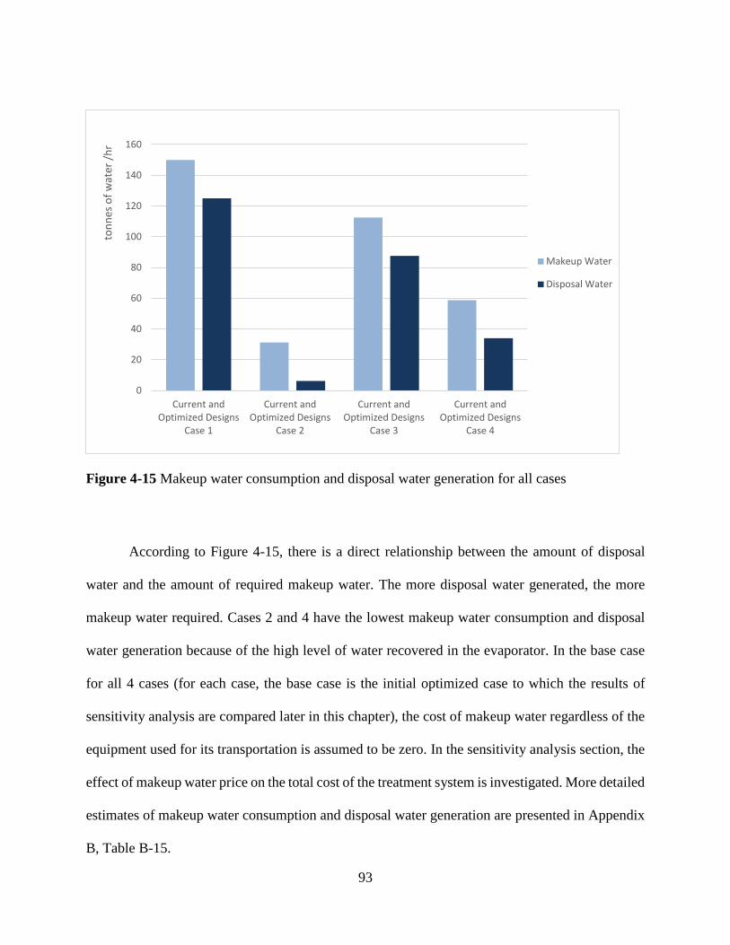
Figure 4-15 Makeup water consumption and disposal water generation for all cases
According to Figure 4-15, there is a direct relationship between the amount of disposal
water and the amount of required makeup water. The more disposal water generated, the more
makeup water required. Cases 2 and 4 have the lowest makeup water consumption and disposal
water generation because of the high level of water recovered in the evaporator. In the base case
for all 4 cases (for each case, the base case is the initial optimized case to which the results of
sensitivity analysis are compared later in this chapter), the cost of makeup water regardless of the
equipment used for its transportation is assumed to be zero. In the sensitivity analysis section, the
effect of makeup water price on the total cost of the treatment system is investigated. More detailed
estimates of makeup water consumption and disposal water generation are presented in Appendix
B, Table B-15.
0
20
40
60
80
100
120
140
160
Current andOptimized Designs
Case 1
Current andOptimized Designs
Case 2
Current andOptimized Designs
Case 3
Current andOptimized Designs
Case 4
tonn
es o
f wat
er /h
r
Makeup Water
Disposal Water
93
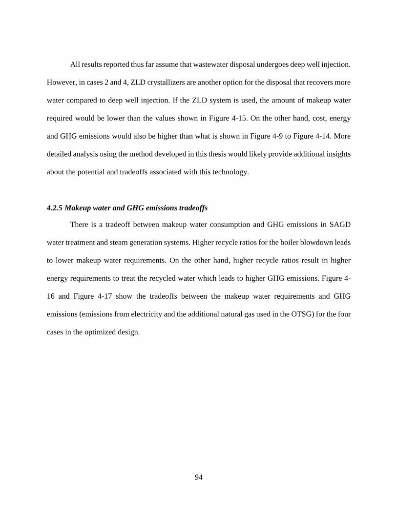
All results reported thus far assume that wastewater disposal undergoes deep well injection.
However, in cases 2 and 4, ZLD crystallizers are another option for the disposal that recovers more
water compared to deep well injection. If the ZLD system is used, the amount of makeup water
required would be lower than the values shown in Figure 4-15. On the other hand, cost, energy
and GHG emissions would also be higher than what is shown in Figure 4-9 to Figure 4-14. More
detailed analysis using the method developed in this thesis would likely provide additional insights
about the potential and tradeoffs associated with this technology.
4.2.5 Makeup water and GHG emissions tradeoffs
There is a tradeoff between makeup water consumption and GHG emissions in SAGD
water treatment and steam generation systems. Higher recycle ratios for the boiler blowdown leads
to lower makeup water requirements. On the other hand, higher recycle ratios result in higher
energy requirements to treat the recycled water which leads to higher GHG emissions. Figure 4-
16 and Figure 4-17 show the tradeoffs between the makeup water requirements and GHG
emissions (emissions from electricity and the additional natural gas used in the OTSG) for the four
cases in the optimized design.
94
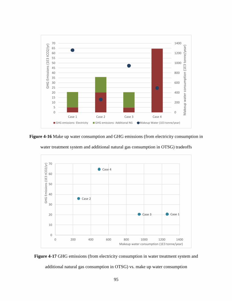
Figure 4-16 Make up water consumption and GHG emissions (from electricity consumption in
water treatment system and additional natural gas consumption in OTSG) tradeoffs
Figure 4-17 GHG emissions (from electricity consumption in water treatment system and
additional natural gas consumption in OTSG) vs. make up water consumption
0
200
400
600
800
1000
1200
1400
05
10152025303540455055606570
Case 1 Case 2 Case 3 Case 4
Mak
eup
wat
er c
onsu
mpt
ion
(1E3
tonn
e/ye
ar)
GHG
Emiss
ions
(1E3
tCO
2/yr
)
GHG emissions- Electricity GHG emissions- Additional NG Makeup Water (1E3 tonne/year)
Case 1
Case 2
Case 3
Case 4
0
10
20
30
40
50
60
70
0 200 400 600 800 1000 1200 1400
GHG
Emiss
ions
(1E3
tCO
2/yr
)
Makeup water consumption (1E3 tonne/year)
95
Cases 1 and 3 have high makeup water requirements and low GHG emissions, while case
4 has low makeup water consumption and high GHG emissions. However, in case 2 both makeup
water consumption and GHG emissions are relatively low (although GHG emissions in case 2 are
higher than cases 1 and 3, they are still relatively low).
Figure 4-17 shows the water-emission tradeoffs even more clearly. As shown in this figure,
cases 1 and 3 are low in emissions and case 4 is low in water use and case 2 is in-between. We are
aiming towards the lower left quadrant of the figure. None of the options really fit in this quadrant
so the decision is really between cases 2 and 3 if these are the only two metrics that we care about.
Case 2 is recommended if makeup water is the priority whereas case 3 is recommended if GHG
emissions are your priority.
As shown in Figure 4-16 and Figure 4-17, the makeup water consumption in case 3 is
reduced by 25% compared to case 1 by recycling 30% of the OTSG blowdown to the treatment
system, and GHG emissions are only increased by 7%. The effect of the blowdown recycle ratio
on water consumption and GHG emissions is further investigated in the sensitivity analysis
section.
4.3 Energy minimization analysis for the treatment network
The model can also be run to minimize energy (instead of cost). The results of the energy
minimization runs show that the same amount of electricity is consumed regardless of which
objective function is selected. This means that the electricity savings achieved by cost optimization
is the maximum amount of savings that can be reached in the system using optimization techniques
and the current configuration of the model. Further electricity savings require process
modifications or switching to other water treatment processes.
96

Since the results of energy minimization are similar to the results of cost minimization (less
than 1% difference in the cost, energy consumption, GHG emissions, etc.), they are not presented
here.
4.4 Sensitivity analysis
There is a high degree of uncertainty in the data in this thesis (e.g., performance and
limitations of the treatment units, source of electricity, cost data, etc.). Therefore, a sensitivity
analysis is conducted to better understand the parameters that have the largest impact on estimates
of cost, energy and emissions for the different cases considered. The impacts of many parameters
have been investigated in the model and the most interesting results are presented here.
4.4.1 Hardness requirement in the boiler
The hardness requirement in the OTSG feed water is assumed to be 3 ppm in the base case
(for cases 1, 2 and 3), that is the most common value for hardness requirement in the OTSG
reported in the literature [8], [23]. In the sensitivity analysis, 1 ppm and 10 ppm are investigated
as hardness requirements in the boiler based on consultation with experts [94]. The results are
similar for all three cases (1, 2, and 3).
The current design doesn’t change by changing the hardness requirement in the boiler,
because in the current design all produced water passes through all of the treatment units regardless
of the performance of the treatment units and the concentration requirements in the boiler. The
results show that the hardness concentration required for the boiler feed water doesn’t have a
significant effect on the total cost of the water treatment system and the cost savings potential via
optimization. The total cost of the treatment system slightly reduces (less than 1%) as the hardness
97

concentration required in the boiler increases. According to the results, the small reduction in costs
is due to a reduction in chemical costs rather than the electricity and other costs. The reason is that
the ion exchange unit that is responsible for hardness removal, uses chemicals (Na2CO3, NaOH,
HCl) to remove the hardness and chemical costs are the most significant contributor (99% of the
total operating cost of the ion exchange unit) to the total operating cost of this treatment unit.
Therefore, when the hardness concentration requirement is lower or higher compared to the base
case, more or less flow needs to go through this treatment unit respectively which affects the
chemicals requirements and chemicals cost (by about 4%) and consequently the total operating
cost (by less than 1%). Similar results are obtained for the capital cost and the capital cost savings.
The effect of hardness requirements in the boiler on the electricity consumption and GHG
emissions are negligible (i.e., < 0.5%).
4.4.2 Silica requirement in the boiler
The required silica concentration in the OTSG is 50 ppm in the base case (the most common
value reported in the literature for silica requirement in the OTSG [8], [23]). In the sensitivity
analysis, 30 ppm and 70 ppm are tested based on consultation with experts (for cases 1, 2 and 3).
The total cost of the treatment system changed by about -4% to +5% for case 1, -5% to +7% for
case 2 and -3% to +6% for case 3 (the total cost decreases when the silica requirements increase
and the total cost increases when the silica requirements decreases). The changes in the cost
savings is due to the different flow rates of the inlet stream to the lime softening unit (the treatment
unit that removes silica from the wastewater).
98
Since the lime softening unit is more expensive than the ion exchange unit, changing the
silica requirements in the boiler has a greater effect on the cost of the treatment system than
changing the hardness requirements (in the previous section).
In all three cases 28 ppm is approximately the lowest silica concentration that can be
reached by the lime softener with the data used in the model. By lowering the silica requirement
beyond this point in the OTSG, the optimization model chooses the evaporator instead of the lime
softener. Therefore, 28 ppm can be considered the transition point for the silica concentration to
switch from the lime softener to the evaporator.
4.4.3 Capital cost of the treatment units
To study the effect of uncertain and variable capital costs of the treatment units on the
optimal design and the total cost of the water treatment system, for the capital cost of the treatment
units in the base case, multipliers are used that range from 0.5 to 1.5 (steps of 0.1: 0.5, 0.6, etc.).
This is because capital cost may be affected by the geographical location where the project is being
executed (due to different equipment prices in different regions and countries. For example, in
Alberta higher prices exist because of the high labor cost).The optimal design and the total cost of
the treatment system are obtained for each multiplier for all four cases.
The results show that applying a multiplier for the capital cost increases the total cost of
the treatment system linearly. Although the cost savings increases for the larger multipliers
(between 2-9% in each step), there is not a significant change in the percentage of cost savings
(about 2%). The results of the optimization show that the optimal design of the treatment system
(the treatment system configuration and flow rates) doesn’t change due to any multiplier
considered.
99

4.4.4 Boiler blowdown recycle ratio in case 3
In the base case of case 3, 30% of the boiler blowdown is recycled back to the treatment
system for further treatment and reuse in the boiler. The effect of changing the boiler blowdown
recycle ratio to 20% and 50% on the total cost of the treatment system and makeup water
consumption is investigated.
The recycling ratio also raises further tradeoffs between the cost/electricity use/GHG
emissions and water use. Makeup water requirements and disposal water generated for different
boiler blowdown recycle ratios are shown in Figure 4-18.
Figure 4-18 Effect of boiler blowdown recycle ratio on makeup water consumption and disposal
water generation in case 3
0
20
40
60
80
100
120
140
Case 3- 20% recycle Case 3- 30% recycle Case 3- 50% resycle
tonn
es o
f wat
er/h
r
Makeup Water
Disposal Water
100
Recycling 50% of boiler blowdown, reduces the need for makeup water (reductions on the
order of 10-22% below the cases where 30% is assumed). On the other hand, recycling more
blowdown requires more treatment which increases energy use, GHG emissions and cost. The total
optimal cost of the treatment system, electricity consumption and GHG emissions slightly increase
(1.6-3.5%) by increasing the boiler blowdown recycle ratio from 30 to 50%.
A sensitivity analysis was done on the makeup water cost. By comparing the 50% recycle
case to the base case (30% recycle), it is seen that by assigning a 2.3 ($/tonne of water) price to
the makeup water, the cost of the two cases will be the same. In other words, at costs below 2.3
$/tonnes of water, 50% recycle is more expensive than 30% recycle and at costs above 2.3 $/tonnes
of water, 50% recycle is cheaper than 30% recycle.
4.4.5 Makeup water price
The total cost of the water treatment system in case 3 is relatively low and the amount of
makeup water consumption is high. On the other hand, the total cost of the water treatment system
in case 4 is high and the makeup water consumption in this case is low (total cost of the water
treatment system in cases 3 and 4 are $1.1E07/year and $2.5E07/year respectively and makeup
water consumption in cases 3 and 4 are 112.5 tonne/hr and 59 tonne/hr respectively). Therefore, I
performed a sensitivity analysis on the cost of makeup water for these two cases.
The results of the sensitivity analysis show that if the price of makeup water was $30.5 per
tonne of water or $0.035 per litre of water, the total cost of the treatment system for these two
cases would be the same. In other words, at costs below $0.035 per litre of water, case 4 is more
expensive than case 3 and at costs above $0.035 per litre of water, case 3 is more expensive.
Generally, the average fresh water consumption in SAGD operations is approximately 0.5 barrels
101

of fresh water per barrel of oil produced [29]. The calculated price for the makeup water ($0.035
per litre of water) results in an additional cost of $1.47 per barrel oil produced.
Under some reservoir conditions, excess water is produced in the SAGD process that will
reduce the makeup water requirements and the total cost of the system. The model is capable of
incorporating this situation and the amount of excess water produced can be specified in the model
as an input variable.
4.4.6 Makeup water composition
The effect of changing the makeup water composition on the optimized design and total
cost of the water treatment system is investigated here. Makeup water required in the SAGD
operations can be from fresh or brackish (saline) water sources (brackish water has higher hardness
concentrations (about 10 times higher than fresh water). In the base case of all the four cases,
makeup water is assumed to be from a fresh water source. In the sensitivity analysis brackish water
is considered as the source of makeup water. The results show that the total cost increases by less
than 1% when brackish water is used. The cost increase is due to a 2-8% increase in the flow rate
of the inlet stream to the WAC unit which is responsible for hardness removal in the water
treatment system.
4.4.7 Inlet oil concentration limit for the oil removal filter
The effect of different inlet oil concentration limits for the oil removal filter has been
investigated. The results show that the optimal design doesn’t change by changing the inlet oil
limit of ORF and this parameter is not a significant parameter affecting the total cost of the water
treatment system (total cost of the water treatment system changes less than 1%).
102

4.4.8 Electricity emissions intensity
In the base case, the electricity emissions factor is assumed to be 0.75 tCO2/MWh for the
Alberta grid [102]. However, this value changes greatly from year to year. In addition, the future
Alberta electricity grid could employ very different generation types. A sensitivity analysis to
investigate the effect of the electricity emissions factor on the total GHG emissions (from
electricity and additional natural gas in the OTSG) over a range of 0-1 tCO2/MWh for the
electricity emissions factor is conducted (0 represents electricity production from renewable
sources that are close to 0 tCO2/MWh and 1 refers to electricity production from coal).
Figure 4-19 Effect of the electricity emissions factor on the total GHG emission (from electricity
consumption in water treatment system and additional natural gas in the OTSG)
0
10
20
30
40
50
60
70
80
90
100
0 0.2 0.4 0.6 0.8 1 1.2
GHG
emiss
ions
(ele
ctric
ity a
nd a
dded
NG)
(10E
3 t/
year
)
Electricity Emissions Factor (tCO2/MWh electricity)
Cases 1 and 3
Case 2
Case 4
103

As shown in Figure 4-19, for lower values of electricity emissions factor, case 4 has lower
GHG emissions, but by increasing this value, the total GHG emissions of case 4 increases more
rapidly than the three other cases. The reason is the electricity consumption of case 4 is
significantly higher than other cases and total GHG emissions in this case is affected more
significantly by increasing the electricity emission factor. According to Figure 4-19, at emissions
factor of approximately 0.26 tCO2/MWh, the total emissions of case 4 is equal to case 2. Before
this point case 2 has higher emissions and after this point emissions in case 4 overtake case 2 which
means that when electricity is generated from clean sources of energy (e.g., renewable and nuclear
energy), case 4 has the lowest GHG emissions among all four cases, but with electricity generated
from emission intensive sources (e.g., coal, natural gas, etc.), case 4 has higher GHG emissions
than the other three cases.
4.4.9 Carbon tax
Environmental regulations are trying to push industries towards lower carbon emissions
[104]. A carbon tax which is usually defined as placing a fee on GHG emissions is one of the
solutions that can incentivize industries to reduce their emissions [105]. To investigate the impact
of a carbon tax on decision making about the water treatment technologies used in a SAGD water
treatment system, a sensitivity analysis is done to assess the effect of carbon price on the total cost
of a SAGD plant. In the base case, the carbon tax is considered to be zero. The sensitivity analysis
is done by increasing the carbon tax from $0 to $150/tonneCO2. The results are shown in Figure
4-20.
104
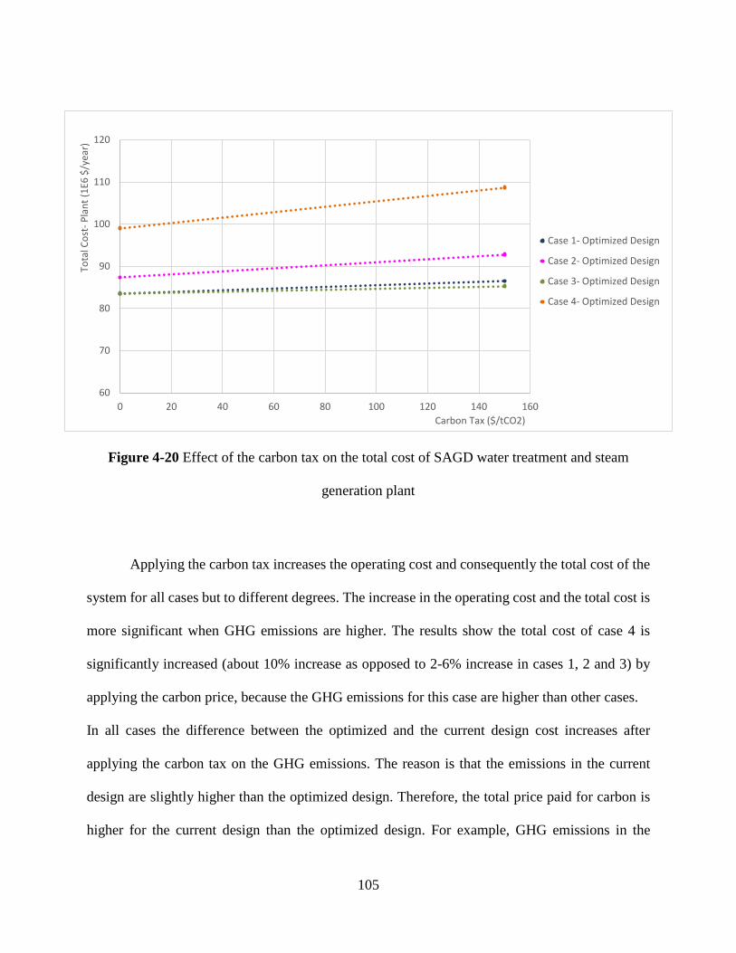
Figure 4-20 Effect of the carbon tax on the total cost of SAGD water treatment and steam
generation plant
Applying the carbon tax increases the operating cost and consequently the total cost of the
system for all cases but to different degrees. The increase in the operating cost and the total cost is
more significant when GHG emissions are higher. The results show the total cost of case 4 is
significantly increased (about 10% increase as opposed to 2-6% increase in cases 1, 2 and 3) by
applying the carbon price, because the GHG emissions for this case are higher than other cases.
In all cases the difference between the optimized and the current design cost increases after
applying the carbon tax on the GHG emissions. The reason is that the emissions in the current
design are slightly higher than the optimized design. Therefore, the total price paid for carbon is
higher for the current design than the optimized design. For example, GHG emissions in the
60
70
80
90
100
110
120
0 20 40 60 80 100 120 140 160
Tota
l Cos
t-Pl
ant (
1E6
$/ye
ar)
Carbon Tax ($/tCO2)
Case 1- Optimized Design
Case 2- Optimized Design
Case 3- Optimized Design
Case 4- Optimized Design
105

optimized design of case 3 are 5.5E02 tCO2/year lower than the current design. Total cost of the
plant for current and optimized designs of case 3 are $8.7E07/year and $8.5E07/year respectively
with zero carbon tax and $9.0E07/year and $8.7E07/year with $150/tonneCO2 carbon tax. This
means that the cost difference of the plant between the current and optimized designs has increased
by 4% when the carbon tax is $150/tonneCO2 compared to zero carbon tax.
106
Chapter Five: Conclusions and Recommendations
5.1 Summary of results and principal insights
This study shows that process integration techniques can demonstrate potential cost and
energy savings in the water treatment system of SAGD operations. Results of the study show up
to 19.5% cost savings (for water treatment system cost in case 1) and up to 12% electricity savings
(for electricity consumption in water treatment system in case 1) only by diverting flows in
wastewater streams. According to the results, lime softening and evaporator units have the most
significant contribution to the cost and energy savings.
In this study the effect of using treatment alternatives in the SAGD water treatment system
is also investigated by considering four different cases for water treatment and steam generation
system in SAGD operations. According to the results, from a cost perspective, cases 1 and 3 (with
no evaporator) are the most attractive cases. Case 4 (produced water evaporation) is the most
expensive case and case 2 (blowdown evaporation) lies in-between. From an energy consumption
and GHG emissions perspective, again cases 1 and 3 are the best cases with the lowest energy
consumption and GHG emissions. Although case 4 consumed the most electricity, total energy
consumption (electricity and natural gas in boiler) of case 2 is about 18% higher than the total
energy consumption of case 4. However, total GHG emissions from case 4 is higher than case 2
because of the significant share of electricity in total energy consumption (electricity emission
factor is calculated from Alberta’s electricity grid and is much higher than that of natural gas).
From a water consumption perspective, case 2 is the most favourable case having the lowest water
consumption. Cases 1 and 3 have the highest water consumption and case 4 lies in-between.
107
There are tradeoffs between cost, energy, emissions and water. Choosing the best case
depends on how water, energy and GHG emissions are valued. For example, when the price of
makeup water is zero, case 2 is more expensive than cases 1 and 3, but if the makeup water price
is greater than 0.7 ¢/litre, case 2 becomes cheaper than cases 1 and 3. Also, total GHG emissions
of case 2 are higher than cases 1 and 3 in the base case (where electricity emission factor is
calculated for Alberta’s electricity grid- 0.75 tCO2/MWh electricity), but when lower carbon
sources of electricity are used, the difference between the total emissions of case 2 and cases 1 and
3 is very small and for zero carbon electricity, the total emissions of cases 1, 2 and 3 are the same.
That is to say, the choice of the best configuration for the water treatment system of SAGD
operations depends on several factors such as makeup water price, carbon intensity of the
electricity, etc. It also depends on the importance placed on minimizing water, GHG emissions
and cost for decision makers, based on which the suitableness of an option can be determined, and
there is no single treatment configuration that consistently gives the best results.
Currently, water is highly undervalued and oil sands producers pay negligible prices for
withdrawing water for extraction purposes. Placing a price on water could move the SAGD
projects towards less water intensive options (e.g., use of evaporators). However, in several cases
the price would have to be potentially prohibitively high (e.g., $1.47/bbl of oil produced) in order
to see a change in investment decision towards a less water intensive option. In addition, the use
of technologies such as evaporators come with important tradeoffs between cost, water, and GHG
emissions. In the face of these tradeoffs, a range of policy alternatives (e.g., price on water,
withdrawal and disposal requirements) should be explored to find the best balance between cost,
energy, GHG emissions and water.
108
5.2 Future work
There are several options to expand the current study into a more comprehensive work. For
instance, this work can be blended with energy integration studies and expanded to a simultaneous
water and energy minimization model using process integration tools. Linear cost functions are
assumed in this study, but the model is capable of using nonlinear cost functions as well. Nonlinear
cost functions may better represent the costs of some of the treatment units, and improve the
accuracy of the results of the study. Additionally, although piping costs and the distances between
the treatment units are not considered in this study (required data were not available), if the data
related to piping costs and distances between the treatment units are available, they can be
incorporated in the model to improve the accuracy of the results.
There are many treatment processes (membranes, hydrocyclones, etc.) that can be used for
water treatment in SAGD facilities and have not yet been investigated. These treatment processes
need to be further investigated by oil sands producers to determine their suitability for use in the
SAGD operations. The proposed model in this study can help investigate new water treatment
technologies and find the tradeoffs between water, energy, emissions and cost associated with
various groups of technologies and help the oil sands operators gain a better understanding of the
advantages and disadvantages of their possible choices.
5.3 Recommendations
The framework developed in this study can help oil sands operators make informed
decisions about which water treatment technologies to choose for SAGD operations. For example,
if cost is the most determinative factor, conventional treatment technologies, lime softening and
ion exchange, are better choices compared to evaporators. But if reducing water consumption is
109
the most important factor in the decision making process, the use of evaporators would be a better
option to reduce water consumption and disposal. If reducing GHG emissions is more important
than cost and water consumption, each of four different cases could be the best choice depending
on the electricity emission factor, and conducting sensitivity analysis can help the operators find
the best option in various circumstances.
110
References
[1] F. Birol and others, “World energy outlook,” Paris Int. Energy Agency, 2008.
[2] bp.com/energyoutlook, “Energy Outlook 2035 booklet.”
[3] “International Energy Agency.” [Online]. Available: http://www.iea.org/. [Accessed: 02-
Oct-2014].
[4] G. Tverberg, “World Energy Consumption Since 1820 in Charts,” Our Finite World. .
[5] V. Smil, Energy Transitions: History, Requirements, Prospects. Santa Barbara, Calif:
Praeger, 2010.
[6] EIA, “International Energy Statistics,” Independent Statistics & Analysis, U.S. Energy
Information Administration. [Online]. Available:
http://www.eia.gov/cfapps/ipdbproject/iedindex3.cfm?tid=44&pid=44&aid=2&cid=ww,&
syid=1980&eyid=2012&unit=QBTU. [Accessed: 08-Dec-2014].
[7] “Alberta Oil Sands Industry Quarterly Update - Summer2014,” Jun. 2014.
[8] K.-W. Gwak and W. Bae, “A Review of Steam Generation for In-Situ Oil Sands Projects,”
Geosystem Eng., vol. 13, no. 3, pp. 111–118, Sep. 2010.
[9] “Crude Oil Price History Chart,” MacroTrends- Economic Charts and Analysis. [Online].
Available: http://www.macrotrends.net/1369/crude-oil-price-history-chart. [Accessed: 30-
Jan-2015].
[10] International Energy Agency (IEA), “Oil Market Report,” International Energy Agency
(IEA), Oct. 2014.
[11] H. Kawaguchi, Z. Li, Y. Masuda, K. Sato, and H. Nakagawa, “Dissolved organic
compounds in reused process water for steam-assisted gravity drainage oil sands
extraction,” Water Res., vol. 46, no. 17, pp. 5566–5574, Nov. 2012.
111
[12] Rob Engelhardt and Marius Todirescu, “An Introduction to Development in Alberta’s Oil
Sands,” University of Alberta School of Business, Feb. 2005.
[13] L. L. Schramm, Ed., Surfactants: Fundamentals and Applications in the Petroleum
Industry, Reissue edition. Cambridge; New York: Cambridge University Press, 2010.
[14] R. Butler, “Application of SAGD, related processes growing in Canada,” vol. 99, no. 20,
p. p. 74, 2001.
[15] Alberta Energy Regulator, “ST98-2014, Alberta’s Energy Reserves 2013 and
Supply/Demand Outlook 2014–2023,” Alta. Energy Regul., p. 289.
[16] Christopher Holly, Martin Mader, and Jesse Toor, “Oil Sands Production Profile.” Alberta
Department of Energy, 2012.
[17] “Alberta Oil Sands Industry Quarterly Update - Summer2011,” Jun. 2011.
[18] Alberta Energy Regulator, “Directive 081: Water Disposal Limits and Reporting
Requirements for Thermal In Situ Oil Sands Schemes,” Alberta Energy Regulator, Nov.
2012.
[19] W. H. Goodman, M. R. Godfrey, T. M. Miller, and N. Comany, “Scale and deposit
formation in steam assisted gravity drainage (SAGD) facilities,” in Presented at the
International Water Conference, San Antonio, Texas, 2010.
[20] Vicki Lightbown, “New SAGD Technologies Show Promise in Reducing Environmental
Impact of Oil Sand Production.pdf,” Oil Gas Min. Ind. J., vol. 1, no. 2, Mar. 2014.
[21] P. Gosselin, S. E. Hrudey, M. A. Naeth, A. Plourde, R. Therrien, G. Van Der Kraak, and
Z. Xu, “Environmental and health impacts of Canada’s oil sands industry,” 2010.
[22] N. M. Nadella, “Improving Energy Efficiency in Thermal Oil Recovery,” in Improving
Energy Efficiency in Thermal Oil Recovery, Montreal, 2010.
112

[23] P. Pedenaud, C. Goulay, and P. Michaud, “Oily Water Treatment Schemes for Steam
Generation in SAGD heavy oil developments,” 2005.
[24] R. Hill, “Thermal In Situ Water Conservation Study, A Summary Report,” Jacobs
Consultancy, May 2012.
[25] J. Zhou, “Energy-Water Nexus in SAGD: Finding the Right Balance,” CHOA Edmonton
Chapter, 25-Sep-2012.
[26] S. Parab, “Minimizing the Water Usage for Thermal In Situ Oil Sands Schemes- Trade-off
and Challenges,” presented at the CHOA Presentation, 29-Oct-2009.
[27] Government of Alberta, “Specified Gas Emitters Regulations- Alberta Regulation.”
Alberta Queen’s Printer, 2007.
[28] Jacobs Consultancy, “SAGD Energy Efficiency Study,” Alberta Energy Research
Institute, Sep. 2009.
[29] A. Halari, G. Jergeas, and P. Eng, “Lessons Learned from Execution of Oil Sands’ SAGD
Projects,” 2011.
[30] D. Peterson, “Guidelines for Produced Water Evaporators in SAGD,” 2007.
[31] B. Heins, “Operational Experience of Heavy Oil Produced Water Evaporation System at
Suncor Firebag and Deer Creek Facilities in Northern Alberta,” presented at the 2006
CONRAD Water Usage Workshop and Seminar, Ft. McMurray, Alberta, 28-Mar-2006.
[32] Wayne Gilraine, “SAGD Facility Water Treatment and Steam Generation Process
Technology Selection,” Canadian Heavy Oil Association.
[33] M. J. Plebon, “De-Oiling Produced Water from Upstream Operations Without the Need
for Added Chemicals or Heat.pdf,” presented at the PTAC- 2006 Water Innovation in the
Oil Patch Conference, 2006.
113

[34] E. W. Allen, “Process water treatment in Canada’s oil sands industry: I. Target pollutants
and treatment objectives,” J. Environ. Eng. Sci., vol. 7, no. 2, pp. 123–138, Feb. 2008.
[35] BlackPearl Resources Inc. Calgary, Alberta, “Application for Approval of the BlackPearl
Resources Inc. Blackrod Commercial SAGD Project,” May 2012.
[36] James C. Robinson, “An Overview of Produced Water Treatment Technologies,”
presented at the Exploration & Production Technology, delivering breakthrough solutions,
08-Nov-2007.
[37] Rafael Gay-de-Montella, “Water - HC Separation in Alberta Heavy Oil Extraction
Process,” presented at the APEGGA, Nov-2009.
[38] T. Hayes and D. Arthur, “Overview of emerging produced water treatment technologies,”
in 11th Annual International Petroleum Conference, Albuquerque, NM, 2004.
[39] E. T. Igunnu and G. Z. Chen, “Produced water treatment technologies,” Int. J. Low-
Carbon Technol., p. cts049, Jul. 2012.
[40] “Ceramic Membrane Technology,” Canada’s Oil Sands Innovation Alliance. [Online].
Available: http://www.cosia.ca/water. [Accessed: 04-Oct-2014].
[41] Husky Energy, “Oil Sands Water De-Oiling- Challenges and Innovation,” presented at the
Oil Sands Water Management Conference, Calgary, Alberta, 25-Jan-2011.
[42] Erik W. Allen, “Process Water Treatment in the Oil Sands: Emerging water treatment
technologies and their potential application to the oil sands industry.” CANMET,
Dcember-2006.
[43] W. F. Heins, R. McNeill, and S. Albion, “World’s First SAGD Facility Using
Evaporators, Drum Boilers, and Zero Discharge Crystallizers to Treat Produced Water,” J.
Can. Pet. Technol., vol. 45, no. 05, May 2006.
114
[44] W. F. Heins, “Is a Paradigm Shift in Produced Water Treatment Technology Occurring at
SAGD Facilities?,” J. Can. Pet. Technol., vol. 49, no. 01, pp. 10–15, Jan. 2010.
[45] S. ALBION, R. O. B. McNEILL, and W. F. HEINS, “Advancements and Optimization of
SAGD Produced Water Evaporator Designs and Modular Installation Methods–A Case
Study.”
[46] A. Cipollina, G. Micale, and L. Rizzuti, Seawater Desalination, 1 edition. Springer Berlin
Heidelberg, 2009.
[47] R. P. Kalakodimi, M. J. Esmacher, and G. E. Water, “Boiler Chemistry Management
Using Coordinated Approach of Chemicals, Membranes and Online Monitoring,” GE
Water Process Technol, 2009.
[48] M. Bridle, “Treatment of SAGD Produced Waters Without Lime Softening,” 2005.
[49] A. R. Committee and others, “ASME Consensus Documents: Feedwater, Boiler Water,
Steam, and Lay-up of Boiler Systems and Water Chemistry Monitoring,” 2007.
[50] W. Tan, H. J. Marquez, and T. Chen, “Multivariable robust controller design for a boiler
system,” Control Syst. Technol. Ieee Trans. On, vol. 10, no. 5, pp. 735–742, 2002.
[51] J. P. Fanaritis, P. Warren, and J. D. Kimmel, “Review of Once-Through Steam
Generators,” J. Pet. Technol., vol. 17, no. 04, pp. 409–416, Apr. 1965.
[52] A. Zaidi and G. Leopold, “Produced Water Treatment - Theory and Practice,” CANMET,
Energy, Mines and Resourced.
[53] GE Water & Process Technologies, “Zero Liquid Discharge Brochure.” General Electric
Company, 2009.
115

[54] Samuel J. Griffin, Karen E. Schooley, and Robert L. Solomon, “The Advantage of Mixed
Salt Crytallizers in Zero Liquid Discharge (ZLD) Wastewater Treatment Sytems.” GE
Power & Water, 2011.
[55] Basil Perdicakis, “SAGD Water Disposal Options, Associated Impacts, and Strategies to
Improve Environmental Footprint.”
[56] J. C. Lozier, U. G. Erdal, A. F. Lynch, and S. Schindler, “Evaluating traditional and
innovative concentrate treatment and disposal methods for water recycling at Big Bear
Valley, California,” CH2M HILL Rep., 2007.
[57] Southern California Regional Brine-Concentrate Management Study, “Brine-Concentrate
Treatment and Disposal Options Report,” U.S. Department of the Interior Bureau of
Reclamation, Southern California, Oct. 2009.
[58] I. C. Kemp, Pinch Analysis and Process Integration: A User Guide on Process Integration
for the Efficient Use of Energy, 2 edition. Amsterdam ; Boston: Butterworth-Heinemann,
2007.
[59] J. J. Klemeš, P. S. Varbanov, and Z. Kravanja, “Recent developments in process
integration,” Chem. Eng. Res. Des., vol. 91, no. 10, pp. 2037–2053, 2013.
[60] G. R. Nabi Bidhendi, N. Mehrdadi, and S. Mohammadnejad, “Water and Wastewater
Minimization in Tehran Oil Refinery using Water Pinch Analysis,” Int. J. Environ. Res.,
vol. 4, no. 4, pp. 583–594, Nov. 2010.
[61] R. Smith, Chemical Process: Design and Integration, 1 edition. Chichester, West Sussex,
England ; Hoboken, NJ: Wiley, 2005.
[62] CANMET Energy Technology Center, “Pinch Analysis: For the Efficient Use of Energy,
Water and Hydrogen,” 2003.
116
[63] Maryam Mahmoudkhani, “Evaluation Energy and Water Saving Opportunities in SAGD,”
presented at the International Process Integration Jubilee Conference, Gothenburg,
Sweden, Mar-2013.
[64] Carlos E Carreon, Maryam Mahmoudkhani, Alberto Alva-Argaez, and Joule Andrea
Bergerson, “Evaluation of energy efficiency options in SAGD oil sands surface facilities
via process integration,” Appl. Therm. Eng., Oct. 2014.
[65] Y. P. Wang and R. Smith, “Wastewater minimisation,” Chem. Eng. Sci., vol. 49, no. 7, pp.
981–1006, Apr. 1994.
[66] Y.-P. Wang and R. Smith, “Design of distributed effluent treatment systems,” Chem. Eng.
Sci., vol. 49, no. 18, pp. 3127–3145, Sep. 1994.
[67] W.-C. J. Kuo and R. Smith, “Effluent treatment system design,” Chem. Eng. Sci., vol. 52,
no. 23, pp. 4273–4290, Dec. 1997.
[68] W. W. Eckenfelder, J. Patoczka, and A. T. Watkin, Wastewater Treatment. McGraw-Hill,
1985.
[69] P. W. Lankford, W. W. Eckenfelder, and K. D. Torrens, “Reducing wastewater toxicity,”
1988.
[70] T. E. Higgins, Ed., Hazardous Waste Minimization Handbook. Chelsea, Mich: CRC Press,
1989.
[71] L. A. McLaughlin, H. J. McLaughlin, and K. A. Groff, “Develop an Effective Wastewater
Treatment Strategy,” Chem. Eng. Prog., pp. 34–42, Sep. 1992.
[72] P. N. Mishra, L. Fan, L. E. Erickson, A. I. of C. Engineers, and C. S. for C. Engineering,
Application of Mathematical Optimization Techniques in Computer Aided Design of
Wastewater Treatment Systems. American Institute of Chemical Engineers, 1973.
117

[73] D. Tyteca, Y. Smeers, E. Nyns, and L. E. Erickson, “Mathematical modeling and
economic optimization of wastewater treatment plants,” C R C Crit. Rev. Environ.
Control, vol. 8, no. 1–4, pp. 1–89, Dec. 1977.
[74] B. Galan and I. E. Grossmann, “Optimal Design of Distributed Wastewater Treatment
Networks,” Ind. Eng. Chem. Res., vol. 37, no. 10, pp. 4036–4048, Oct. 1998.
[75] C.-H. Huang, C.-T. Chang, H.-C. Ling, and Chang, “A Mathematical Programming Model
for Water Usage and Treatment Network Design,” Ind. Eng. Chem. Res., vol. 38, no. 7,
pp. 2666–2679, Jul. 1999.
[76] M. Gunaratnam, A. Alva-Argáez, A. Kokossis, J.-K. Kim, and R. Smith, “Automated
Design of Total Water Systems,” Ind. Eng. Chem. Res., vol. 44, no. 3, pp. 588–599, Feb.
2005.
[77] Z.-H. Liu, J. Shi, and Z.-Y. Liu, “Design of distributed wastewater treatment systems with
multiple contaminants,” Chem. Eng. J., vol. 228, pp. 381–391, Jul. 2013.
[78] W.-C. Kuo, R. Smith, and C. for P. Integration, A Combined Approach to Water
Minimisation and Effluent Treatment System Design. UMIST, 1996.
[79] R. Hernandez-Suarez, J. Castellanos-Fernandez, and J. M. Zamora, “Superstructure
decomposition and parametric optimization approach for the synthesis of distributed
wastewater treatment networks,” Ind. Eng. Chem. Res., vol. 43, no. 9, pp. 2175–2191,
2004.
[80] N. Takama, T. Kuriyama, K. Shiroko, and T. Umeda, “Optimal water allocation in a
petroleum refinery,” Comput. Chem. Eng., vol. 4, no. 4, pp. 251–258, 1980.
[81] M. J. Box, “A new method of constrained optimization and a comparison with other
methods,” Comput. J., vol. 8, no. 1, pp. 42–52, 1965.
118

[82] I. Quesada and I. E. Grossmann, “Global optimization of bilinear process networks with
multicomponent flows,” Comput. Chem. Eng., vol. 19, no. 12, pp. 1219–1242, Dec. 1995.
[83] A. Alva-Argáez, A. C. Kokossis, and R. Smith, “Wastewater minimisation of industrial
systems using an integrated approach,” Comput. Chem. Eng., vol. 22, Supplement 1, pp.
S741–S744, Mar. 1998.
[84] G. Ocanas and L. W. Mays, “A model for water reuse planning,” Water Resour. Res., vol.
17, no. 1, pp. 25–32, Feb. 1981.
[85] Y. Cohen and D. Allen, “An integrated approach to process waste minimization research,”
J. Hazard. Mater., vol. 29, no. 2, pp. 237–253, Jan. 1992.
[86] W.-C. J. Kuo and R. Smith, “Designing for the Interactions Between Water-Use and
Effluent Treatment,” Chem. Eng. Res. Des., vol. 76, no. 3, pp. 287–301, Mar. 1998.
[87] Z. Ujang, C. L. Wong, and Z. A. Manan, “Industrial wastewater minimization using water
pinch analysis: a case study on an old textile plant,” Water Sci. Technol. J. Int. Assoc.
Water Pollut. Res., vol. 46, no. 11–12, pp. 77–84, 2002.
[88] W. L. Winston, Operations Research: Applications and Algorithms, 4 edition. Belmont,
CA: Cengage Learning, 2003.
[89] T. Sottinen, “ORMS 1020,” 2009.
[90] H. A. Taha, Operations research: an introduction. Pearson/Prentice Hall, 2007.
[91] T. F. Edgar and D. M. Himmelblau, Optimization of chemical processes. McGraw-Hill,
1989.
[92] “COSIA: Canada’s Oil Sands Innovation Alliance,” COSIA’s GHG Challenges, 08-Oct-
2014. [Online]. Available: http://www.cosia.ca/initiatives/greenhouse_gases/ghg-
challenge-statements. [Accessed: 01-Dec-2014].
119
[93] Alberto Alva Argáez, “Integrated Design of Water Systems,” Ph.D. Thesis, UMIST,
Manchester, U.K., 1999.
[94] “Personal communication.”
[95] Y. Sawaragi, H. Nakayama, and T. Tanino, Theory of Multiobjective Optimization.
Academic Press, 1985.
[96] J. Viswanathan and I. E. Grossmann, “A combined penalty function and
outerapproximation method for MINLP optimization : applications to distillation column
design,” Carnegie Institute of Technology, Nov. 1989.
[97] W.-C. J. Kuo and R. Smith, “Design of Water-Using Systems Involving Regeneration,”
Process Saf. Environ. Prot., vol. 76, no. 2, pp. 94–114, May 1998.
[98] F. Palacios-Gomez, L. Lasdon, and M. Engquist, “Nonlinear Optimization by Successive
Linear Programming,” Manag. Sci., vol. 28, no. 10, pp. 1106–1120, Oct. 1982.
[99] F. Hutter, H. H. Hoos, and K. Leyton-Brown, “Automated configuration of mixed integer
programming solvers,” in Integration of AI and OR Techniques in Constraint
Programming for Combinatorial Optimization Problems, Springer, 2010, pp. 186–202.
[100] “GAMS World.” [Online]. Available: http://www.gamsworld.org/. [Accessed: 31-Mar-
2015].
[101] “AIMMS -,” AIMMS. [Online]. Available: http://www.aimms.com. [Accessed: 31-Mar-
2015].
[102] “Alberta Energy,” Alberta Energy. [Online]. Available:
http://www.energy.alberta.ca/Electricity/681.asp. [Accessed: 23-Jan-2015].
120

[103] G. H. Doluweera, S. M. Jordaan, M. C. Moore, D. W. Keith, and J. A. Bergerson,
“Evaluating the role of cogeneration for carbon management in Alberta,” Energy Policy,
vol. 39, no. 12, pp. 7963–7974, Dec. 2011.
[104] E. C. Government of Canada, “Copenhagen Accord - Canada’s Action on Climate Change
- Canada’s Action on Climate Change,” 31-Oct-2013. [Online]. Available:
http://climatechange.gc.ca/default.asp?lang=En&n=AA3F6868-1. [Accessed: 25-Jan-
2015].
[105] M. of L. C. S. and O. Government, “What is a Carbon Tax?,” The Province of British
Columbia - Home. [Online]. Available: http://www2.gov.bc.ca/. [Accessed: 25-Jan-2015].
121
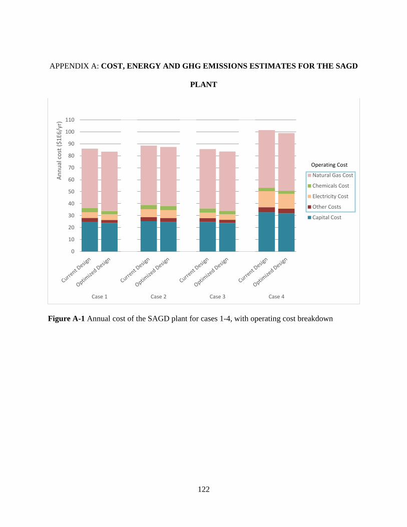
APPENDIX A: COST, ENERGY AND GHG EMISSIONS ESTIMATES FOR THE SAGD
PLANT
Figure A-1 Annual cost of the SAGD plant for cases 1-4, with operating cost breakdown
0
10
20
30
40
50
60
70
80
90
100
110
Case 1 Case 2 Case 3 Case 4
Annu
al c
ost (
$1E6
/yr)
Natural Gas Cost
Chemicals Cost
Electricity Cost
Other Costs
Capital Cost
Operating Cost
122

Table A-1 Capital, operating and total cost of the SAGD plant for current and optimized designs for the four cases (all costs are in $/year)
Case 1 Case 2 Case 3 Case 4
Current Design
Capital Cost 2.49E+07 2.53E+07 2.47E+07 3.28E+07
Operating Cost 6.11E+07 6.33E+07 6.10E+07 6.87E+07
Total Cost 8.60E+07 8.86E+07 8.56E+07 1.02E+08
Optimized Design
Capital Cost 2.40E+07 2.48E+07 2.39E+07 3.19E+07
Operating Cost 5.95E+07 6.26E+07 5.97E+07 6.71E+07
Total Cost 8.35E+07 8.74E+07 8.36E+07 9.90E+07
Table A-2 Capital, operating and total cost savings for the SAGD plant by optimization for the four cases (all costs are in $/year)
Case 1 Case 2 Case 3 Case 4
Total Cost Total Cost Difference 2.53E+06 1.18E+06 2.04E+06 2.49E+06
Total Cost Savings 2.95% 1.33% 2.38% 2.46%
Capital Cost
Capital Cost Difference 9.46E+05 4.99E+05 7.30E+05 8.28E+05
Capital Cost Savings 3.79% 1.97% 2.96% 2.53%
Contribution to total savings 37.30% 42.41% 35.76% 33.23%
Operating Cost
Operating Cost Difference 1.59E+06 6.78E+05 1.31E+06 1.66E+06
Operating Cost Savings 2.60% 1.07% 2.15% 2.42%
Contribution to total savings 62.70% 57.59% 64.24% 66.77%
123

Table A-3 Operating cost of the SAGD plant, broken down into electricity, chemicals and other costs for the four cases (all costs are in $/year)
Case 1 Case 2 Case 3 Case 4
Current Design
Electricity Cost 4.75E+06 6.56E+06 4.64E+06 1.34E+07
Chemicals Cost 3.58E+06 3.61E+06 3.57E+06 2.92E+06
Other Costs 3.20E+06 3.53E+06 3.20E+06 4.25E+06
Optimized Design
Electricity Cost 4.65E+06 6.52E+06 4.56E+06 1.23E+07
Chemicals Cost 2.82E+06 3.27E+06 2.94E+06 2.68E+06
Other Costs 2.46E+06 3.24E+06 2.59E+06 3.88E+06
Table A-4 Electricity, chemicals and other costs savings for the SAGD plant by optimization for the four cases (all costs are in $/year)
Case 1 Case 2 Case 3 Case 4
Electricity
Electricity Cost Difference 9.99E+04 4.22E+04 7.56E+04 1.05E+06
Electricity Cost Savings 2.10% 0.64% 1.63% 7.84%
Contribution in total savings 6.28% 6.23% 5.76% 63.05%
Chemicals
Chemicals Cost Difference 7.53E+05 3.39E+05 6.26E+05 2.40E+05
Chemicals Cost Savings 21.04% 9.41% 17.55% 8.22%
Contribution in total savings 47.35% 50.05% 47.78% 14.40%
Other Costs
Other Costs Difference 7.37E+05 2.96E+05 6.09E+05 3.75E+05
Other Costs Savings 23.05% 8.39% 19.06% 8.82%
Contribution in total savings 46.37% 43.72% 46.46% 22.55%
124

Figure A-2 Annual cost of the SAGD plant for cases 1-4, with capital and operating cost broken down by treatment unit, steam generation and disposal sections (CC=Capital cost- solid fill,
OC=Operating cost- hashed fill)
0
10
20
30
40
50
60
70
80
90
100
110
Case 1 Case 2 Case 3 Case 4
Annu
al c
ost (
$1E6
/yr)
Disposasl
Boiler
Makeup Water
Evaporator
WAC
WLS
ORF
IGF
Skim Tank
CC
OC
125
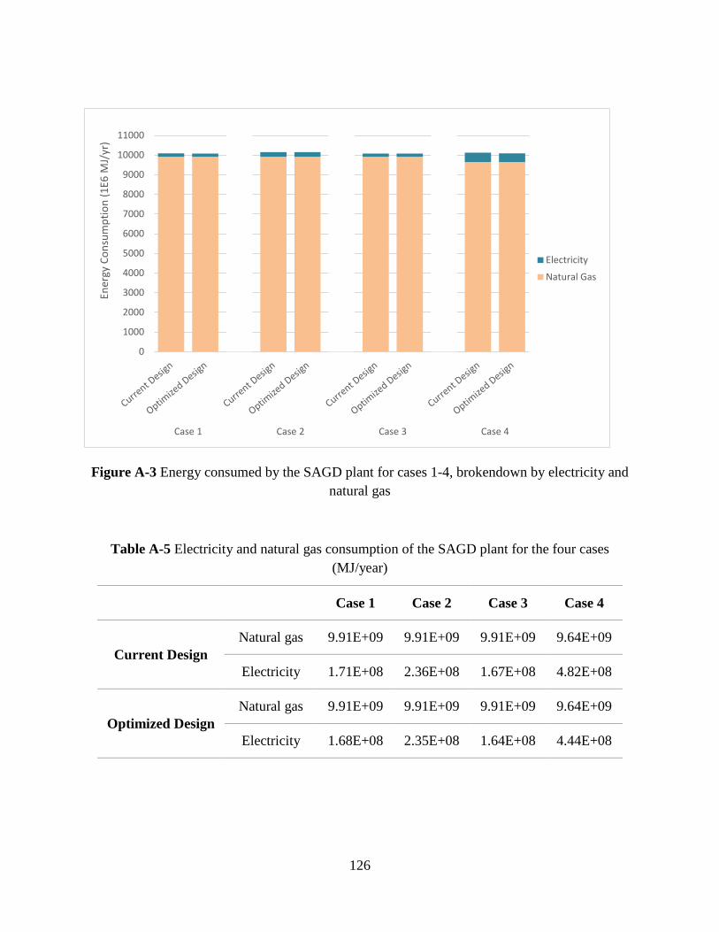
Figure A-3 Energy consumed by the SAGD plant for cases 1-4, brokendown by electricity and natural gas
Table A-5 Electricity and natural gas consumption of the SAGD plant for the four cases (MJ/year)
Case 1 Case 2 Case 3 Case 4
Current Design Natural gas 9.91E+09 9.91E+09 9.91E+09 9.64E+09
Electricity 1.71E+08 2.36E+08 1.67E+08 4.82E+08
Optimized Design Natural gas 9.91E+09 9.91E+09 9.91E+09 9.64E+09
Electricity 1.68E+08 2.35E+08 1.64E+08 4.44E+08
0
1000
2000
3000
4000
5000
6000
7000
8000
9000
10000
11000
Case 1 Case 2 Case 3 Case 4
Ener
gy C
onsu
mpt
ion
(1E6
MJ/
yr)
Electricity
Natural Gas
126

Figure A-4 GHG emissions of the SAGD plant from electricity and natural gas
Table A-6 GHG emissions from electricity and natural gas consumption of the SAGD plant for the four cases (tCO2/year)
Case 1 Case 2 Case 3 Case 4
Current Design GHG emissions- Natural gas 5.61E+05 5.61E+05 5.61E+05 5.46E+05
GHG emissions- Electricity 3.47E+04 4.79E+04 3.39E+04 9.78E+04
Optimized Design GHG emissions- Natural gas 5.61E+05 5.61E+05 5.61E+05 5.46E+05
GHG emissions- Electricity 3.40E+04 4.76E+04 3.33E+04 9.01E+04
050
100150200250300350400450500550600650
Case 1 Case 2 Case 3 Case 4
GHG
Emiss
ions
(1E3
tCO
2/yr
)
GHG Emissions-Electricity
GHG Emissions-Natural Gas
127
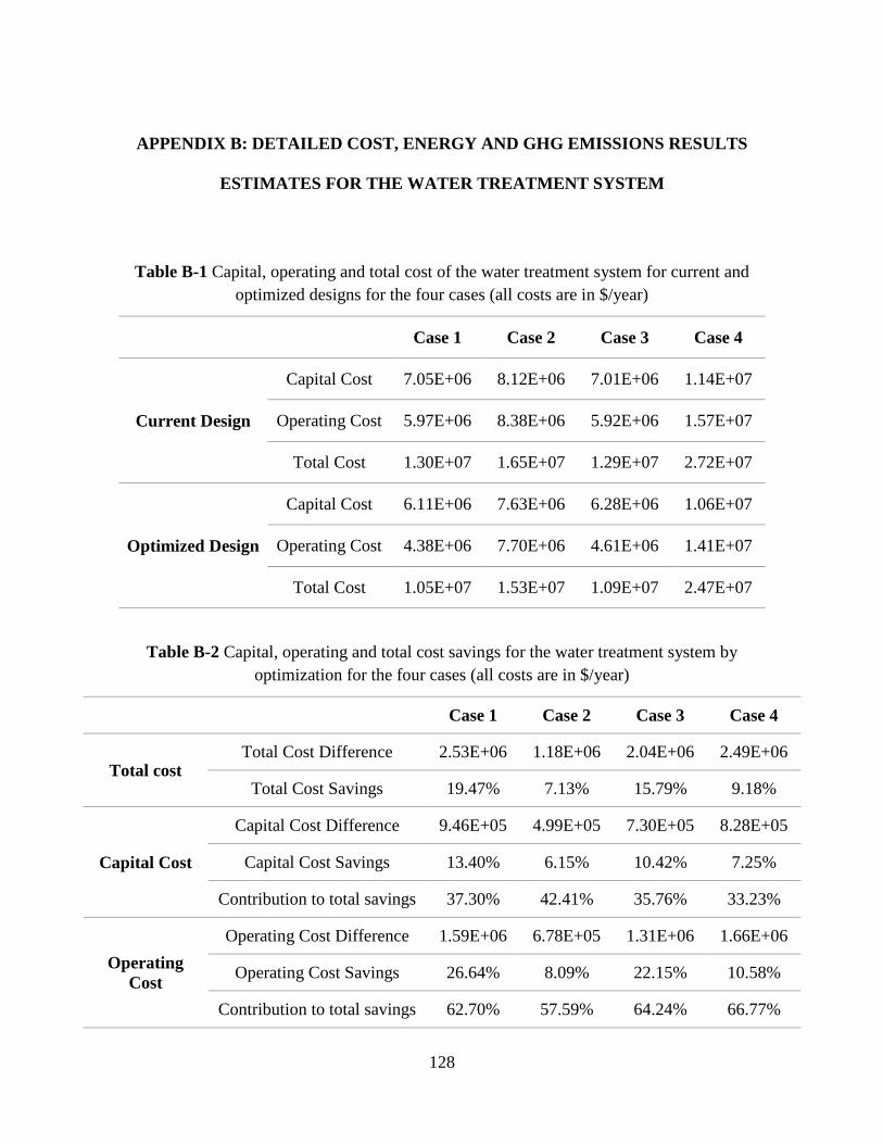
APPENDIX B: DETAILED COST, ENERGY AND GHG EMISSIONS RESULTS
ESTIMATES FOR THE WATER TREATMENT SYSTEM
Table B-1 Capital, operating and total cost of the water treatment system for current and optimized designs for the four cases (all costs are in $/year)
Case 1 Case 2 Case 3 Case 4
Current Design
Capital Cost 7.05E+06 8.12E+06 7.01E+06 1.14E+07
Operating Cost 5.97E+06 8.38E+06 5.92E+06 1.57E+07
Total Cost 1.30E+07 1.65E+07 1.29E+07 2.72E+07
Optimized Design
Capital Cost 6.11E+06 7.63E+06 6.28E+06 1.06E+07
Operating Cost 4.38E+06 7.70E+06 4.61E+06 1.41E+07
Total Cost 1.05E+07 1.53E+07 1.09E+07 2.47E+07
Table B-2 Capital, operating and total cost savings for the water treatment system by optimization for the four cases (all costs are in $/year)
Case 1 Case 2 Case 3 Case 4
Total cost Total Cost Difference 2.53E+06 1.18E+06 2.04E+06 2.49E+06
Total Cost Savings 19.47% 7.13% 15.79% 9.18%
Capital Cost
Capital Cost Difference 9.46E+05 4.99E+05 7.30E+05 8.28E+05
Capital Cost Savings 13.40% 6.15% 10.42% 7.25%
Contribution to total savings 37.30% 42.41% 35.76% 33.23%
Operating Cost
Operating Cost Difference 1.59E+06 6.78E+05 1.31E+06 1.66E+06
Operating Cost Savings 26.64% 8.09% 22.15% 10.58%
Contribution to total savings 62.70% 57.59% 64.24% 66.77%
128

Table B-3 Operating cost of the water treatment system, broken down into electricity, chemicals and other costs for the four cases (all costs are in $/year)
Case 1 Case 2 Case 3 Case 4
Current Design
Electricity Cost 7.86E+05 2.81E+06 7.40E+05 9.89E+06
Chemicals Cost 2.75E+06 2.80E+06 2.75E+06 2.44E+06
Other Costs 2.43E+06 2.77E+06 2.43E+06 3.41E+06
Optimized Design
Electricity Cost 6.86E+05 2.77E+06 6.65E+05 8.84E+06
Chemicals Cost 1.99E+06 2.46E+06 2.12E+06 2.20E+06
Other Costs 1.70E+06 2.47E+06 1.82E+06 3.03E+06
Table B-4 Electricity, chemicals and other costs savings for the water treatment system by optimization for the four cases (all costs are in $/year)
Case 1 Case 2 Case 3 Case 4
Electricity
Electricity Cost Difference 9.99E+04 4.22E+04 7.56E+04 1.05E+06
Electricity Cost Savings 12.71% 1.50% 10.20% 10.61%
Contribution in total savings 6.28% 6.23% 5.76% 63.05%
Chemicals
Chemicals Cost Difference 7.53E+05 3.39E+05 6.26E+05 2.40E+05
Chemicals Cost Savings 27.40% 12.14% 22.81% 9.83%
Contribution in total savings 47.35% 50.05% 47.78% 14.40%
Other Costs
Other Costs Difference 7.37E+05 2.96E+05 6.09E+05 3.75E+05
Other Costs Savings 30.29% 10.70% 25.04% 11.01%
Contribution in total savings 46.37% 43.72% 46.46% 22.55%
129

Table B-5 Operating cost of the water treatment system, broken down by treatment units for the four cases (all costs are in $/year)
Case 1 Case 2 Case 3 Case 4
Current Design
Skim Tank 5.19E+04 5.19E+04 5.19E+04 5.19E+04
IGF 2.29E+05 2.29E+05 2.29E+05 2.29E+05
ORF 0.00E+00 0.00E+00 0.00E+00 0.00E+00
WLS 5.19E+06 4.21E+06 5.19E+06 0.00E+00
WAC 3.09E+05 2.50E+05 3.09E+05 0.00E+00
Evaporator 0.00E+00 3.60E+06 0.00E+00 1.54E+07
Makeup Water 1.81E+05 3.77E+04 1.36E+05 7.09E+04
Optimized Design
Skim Tank 5.19E+04 5.19E+04 5.19E+04 5.19E+04
IGF 2.27E+05 2.27E+05 2.34E+05 2.29E+05
ORF 0.00E+00 0.00E+00 0.00E+00 0.00E+00
WLS 3.62E+06 3.57E+06 3.89E+06 0.00E+00
WAC 2.95E+05 2.08E+05 2.93E+05 2.90E+04
Evaporator 0.00E+00 3.60E+06 0.00E+00 1.37E+07
Makeup Water 1.81E+05 3.77E+04 1.36E+05 7.09E+04
130
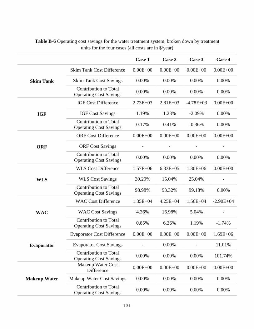
Table B-6 Operating cost savings for the water treatment system, broken down by treatment units for the four cases (all costs are in $/year)
Case 1 Case 2 Case 3 Case 4
Skim Tank
Skim Tank Cost Difference 0.00E+00 0.00E+00 0.00E+00 0.00E+00
Skim Tank Cost Savings 0.00% 0.00% 0.00% 0.00%
Contribution to Total Operating Cost Savings 0.00% 0.00% 0.00% 0.00%
IGF
IGF Cost Difference 2.73E+03 2.81E+03 -4.78E+03 0.00E+00
IGF Cost Savings 1.19% 1.23% -2.09% 0.00%
Contribution to Total Operating Cost Savings 0.17% 0.41% -0.36% 0.00%
ORF
ORF Cost Difference 0.00E+00 0.00E+00 0.00E+00 0.00E+00
ORF Cost Savings - - - -
Contribution to Total Operating Cost Savings 0.00% 0.00% 0.00% 0.00%
WLS
WLS Cost Difference 1.57E+06 6.33E+05 1.30E+06 0.00E+00
WLS Cost Savings 30.29% 15.04% 25.04% -
Contribution to Total Operating Cost Savings 98.98% 93.32% 99.18% 0.00%
WAC
WAC Cost Difference 1.35E+04 4.25E+04 1.56E+04 -2.90E+04
WAC Cost Savings 4.36% 16.98% 5.04% -
Contribution to Total Operating Cost Savings 0.85% 6.26% 1.19% -1.74%
Evaporator
Evaporator Cost Difference 0.00E+00 0.00E+00 0.00E+00 1.69E+06
Evaporator Cost Savings - 0.00% - 11.01%
Contribution to Total Operating Cost Savings 0.00% 0.00% 0.00% 101.74%
Makeup Water
Makeup Water Cost Difference 0.00E+00 0.00E+00 0.00E+00 0.00E+00
Makeup Water Cost Savings 0.00% 0.00% 0.00% 0.00%
Contribution to Total Operating Cost Savings 0.00% 0.00% 0.00% 0.00%
131
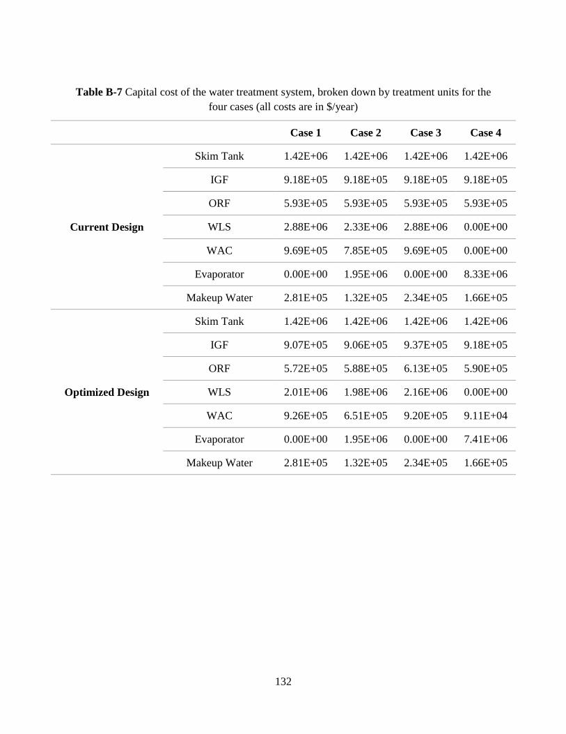
Table B-7 Capital cost of the water treatment system, broken down by treatment units for the four cases (all costs are in $/year)
Case 1 Case 2 Case 3 Case 4
Current Design
Skim Tank 1.42E+06 1.42E+06 1.42E+06 1.42E+06
IGF 9.18E+05 9.18E+05 9.18E+05 9.18E+05
ORF 5.93E+05 5.93E+05 5.93E+05 5.93E+05
WLS 2.88E+06 2.33E+06 2.88E+06 0.00E+00
WAC 9.69E+05 7.85E+05 9.69E+05 0.00E+00
Evaporator 0.00E+00 1.95E+06 0.00E+00 8.33E+06
Makeup Water 2.81E+05 1.32E+05 2.34E+05 1.66E+05
Optimized Design
Skim Tank 1.42E+06 1.42E+06 1.42E+06 1.42E+06
IGF 9.07E+05 9.06E+05 9.37E+05 9.18E+05
ORF 5.72E+05 5.88E+05 6.13E+05 5.90E+05
WLS 2.01E+06 1.98E+06 2.16E+06 0.00E+00
WAC 9.26E+05 6.51E+05 9.20E+05 9.11E+04
Evaporator 0.00E+00 1.95E+06 0.00E+00 7.41E+06
Makeup Water 2.81E+05 1.32E+05 2.34E+05 1.66E+05
132
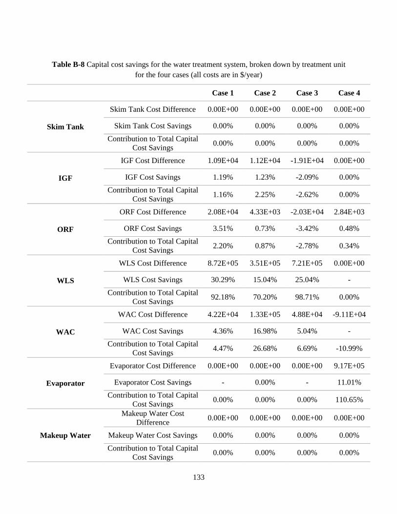
Table B-8 Capital cost savings for the water treatment system, broken down by treatment unit for the four cases (all costs are in $/year)
Case 1 Case 2 Case 3 Case 4
Skim Tank
Skim Tank Cost Difference 0.00E+00 0.00E+00 0.00E+00 0.00E+00
Skim Tank Cost Savings 0.00% 0.00% 0.00% 0.00%
Contribution to Total Capital Cost Savings 0.00% 0.00% 0.00% 0.00%
IGF
IGF Cost Difference 1.09E+04 1.12E+04 -1.91E+04 0.00E+00
IGF Cost Savings 1.19% 1.23% -2.09% 0.00%
Contribution to Total Capital Cost Savings 1.16% 2.25% -2.62% 0.00%
ORF
ORF Cost Difference 2.08E+04 4.33E+03 -2.03E+04 2.84E+03
ORF Cost Savings 3.51% 0.73% -3.42% 0.48%
Contribution to Total Capital Cost Savings 2.20% 0.87% -2.78% 0.34%
WLS
WLS Cost Difference 8.72E+05 3.51E+05 7.21E+05 0.00E+00
WLS Cost Savings 30.29% 15.04% 25.04% -
Contribution to Total Capital Cost Savings 92.18% 70.20% 98.71% 0.00%
WAC
WAC Cost Difference 4.22E+04 1.33E+05 4.88E+04 -9.11E+04
WAC Cost Savings 4.36% 16.98% 5.04% -
Contribution to Total Capital Cost Savings 4.47% 26.68% 6.69% -10.99%
Evaporator
Evaporator Cost Difference 0.00E+00 0.00E+00 0.00E+00 9.17E+05
Evaporator Cost Savings - 0.00% - 11.01%
Contribution to Total Capital Cost Savings 0.00% 0.00% 0.00% 110.65%
Makeup Water
Makeup Water Cost Difference 0.00E+00 0.00E+00 0.00E+00 0.00E+00
Makeup Water Cost Savings 0.00% 0.00% 0.00% 0.00%
Contribution to Total Capital Cost Savings 0.00% 0.00% 0.00% 0.00%
133
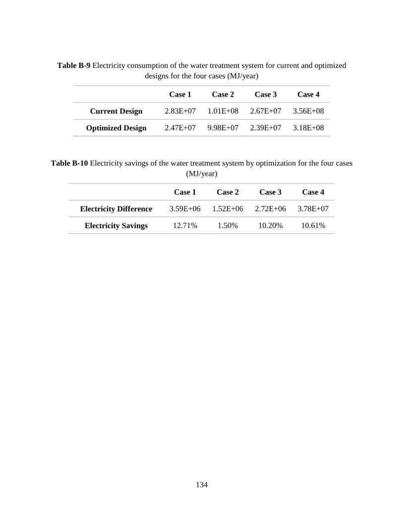
Table B-9 Electricity consumption of the water treatment system for current and optimized designs for the four cases (MJ/year)
Case 1 Case 2 Case 3 Case 4
Current Design 2.83E+07 1.01E+08 2.67E+07 3.56E+08
Optimized Design 2.47E+07 9.98E+07 2.39E+07 3.18E+08
Table B-10 Electricity savings of the water treatment system by optimization for the four cases (MJ/year)
Case 1 Case 2 Case 3 Case 4
Electricity Difference 3.59E+06 1.52E+06 2.72E+06 3.78E+07
Electricity Savings 12.71% 1.50% 10.20% 10.61%
134
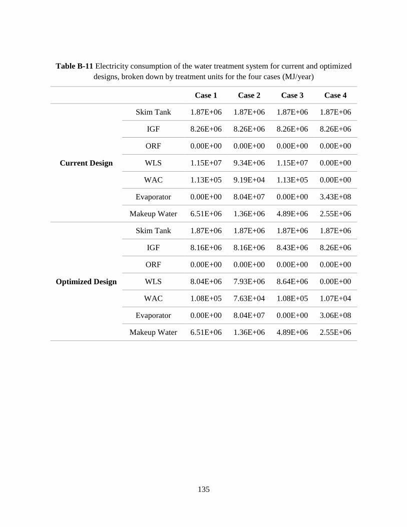
Table B-11 Electricity consumption of the water treatment system for current and optimized designs, broken down by treatment units for the four cases (MJ/year)
Case 1 Case 2 Case 3 Case 4
Current Design
Skim Tank 1.87E+06 1.87E+06 1.87E+06 1.87E+06
IGF 8.26E+06 8.26E+06 8.26E+06 8.26E+06
ORF 0.00E+00 0.00E+00 0.00E+00 0.00E+00
WLS 1.15E+07 9.34E+06 1.15E+07 0.00E+00
WAC 1.13E+05 9.19E+04 1.13E+05 0.00E+00
Evaporator 0.00E+00 8.04E+07 0.00E+00 3.43E+08
Makeup Water 6.51E+06 1.36E+06 4.89E+06 2.55E+06
Optimized Design
Skim Tank 1.87E+06 1.87E+06 1.87E+06 1.87E+06
IGF 8.16E+06 8.16E+06 8.43E+06 8.26E+06
ORF 0.00E+00 0.00E+00 0.00E+00 0.00E+00
WLS 8.04E+06 7.93E+06 8.64E+06 0.00E+00
WAC 1.08E+05 7.63E+04 1.08E+05 1.07E+04
Evaporator 0.00E+00 8.04E+07 0.00E+00 3.06E+08
Makeup Water 6.51E+06 1.36E+06 4.89E+06 2.55E+06
135

Table B-12 Electricity savings of the water treatment system, broken down by treatment units for the four cases (MJ/year)
Case 1 Case 2 Case 3 Case 4
Skim Tank
Skim Tank Electricity Consumption Difference 0.00E+00 0.00E+00 0.00E+00 0.00E+00
Skim Tank Electricity Savings 0.00% 0.00% 0.00% 0.00%
Contribution to Total Electricity Savings 0.00% 0.00% 0.00% 0.00%
IGF
IGF Electricity Consumption Difference 9.84E+04 1.01E+05 -1.72E+05 0.00E+00
IGF Electricity Savings 1.19% 1.23% -2.09% 0.00%
Contribution to Total Electricity Savings 2.74% 6.66% -6.33% 0.00%
ORF
ORF Electricity Consumption Difference 0.00E+00 0.00E+00 0.00E+00 0.00E+00
ORF Electricity Savings - - - -
Contribution to Total Electricity Savings 0.00% 0.00% 0.00% 0.00%
WLS
WLS Electricity Consumption Difference 3.49E+06 1.40E+06 2.89E+06 0.00E+00
WLS Electricity Savings 30.29% 15.04% 25.04% -
Contribution to Total Electricity Savings 97.13% 92.32% 106.12% 0.00%
WAC
WAC Electricity Consumption Difference 4.94E+03 1.56E+04 5.71E+03 -1.07E+04
WAC Electricity Savings 4.36% 16.98% 5.04% -
Contribution to Total Electricity Savings 0.14% 1.03% 0.21% -0.03%
Evaporator
Evaporator Electricity Consumption Difference 0.00E+00 0.00E+00 0.00E+00 3.78E+07
Evaporator Electricity Savings - 0.00% - 11.01%
Contribution to Total Electricity Savings 0.00% 0.00% 0.00% 100.03%
Makeup Water
Makeup Water Electricity Consumption Difference 0.00E+00 0.00E+00 0.00E+00 0.00E+00
Makeup Water Electricity Savings 0.00% 0.00% 0.00% 0.00%
Contribution to Total Electricity Savings 0.00% 0.00% 0.00% 0.00%
136

Table B-13 GHG emissions from electricity consumption of the water treatment system for the four cases (tCO2/year)
Case 1 Case 2 Case 3 Case 4
Current Design 5.74E+03 2.06E+04 5.41E+03 7.22E+04
Optimized Design 5.01E+03 2.02E+04 4.86E+03 6.46E+04
Table B-14 GHG emissions reduction in the water treatment system by optimization for the four cases (tCO2/year)
Case 1 Case 2 Case 3 Case 4
GHG Emissions Difference 7.29E+02 3.09E+02 5.52E+02 7.67E+03
GHG Emissions Reduction 12.71% 1.50% 10.20% 10.61%
Table B-15 Makeup water consumption and disposal water generation in SAGD operations for the four cases (tonne/hr)
Case 1 Case 2 Case 3 Case 4
Makeup Water Consumed 150 31.25 112.5 58.75
Disposal Water Generated 125 6.227 87.5 33.95
137