investigation on lithium ion conductivity and...
TRANSCRIPT

INVESTIGATION ON LITHIUM ION CONDUCTIVITY AND CHARACTERIZATION OF PMMA–PVC BASED POLYMER ELECTROLYTES INCORPORATING IONIC LIQUID AND NANO–
FILLER
By
LIEW CHIAM WEN
A thesis submitted to the Department of Bioscience and Chemistry, Faculty of Engineering and Science,
Universiti Tunku Abdul Rahman, in partial fulfillment of the requirements for the degree of
Master of Science in April 2011

ii
ABSTRACT
INVESTIGATION ON LITHIUM ION CONDUCTIVITY AND CHARACTERIZATION OF PMMA–PVC BASED POLYMER
ELECTROLYTES INCORPORATING IONIC LIQUID AND NANO–FILLER
Liew Chiam Wen
There are four polymer electrolyte systems in this project. First and second
polymeric systems are known as screening steps. Poly(methyl methacrylate)
(PMMA) and poly(vinyl chloride) (PVC) were used as host polymers with lithium
bis(trifluoromethanesulfonyl) imide (LiTFSI) as doping salt. Additives such as 1–
butyl–3–methylimidazolium bis(trifluoromethylsulfonyl imide) (BmImTFSI) ionic
liquid and nano–sized inorganic reinforcement filler, fumed silica (SiO2) were
employed. All the polymer electrolytes are prepared by means of solution casting
technique. PMMA (70 wt%) and PVC (30 wt%) is the most compatible ratio in the
first system. The highest ionic conductivity of 1.60×10⁻⁸ Scm-1 was achieved at
ambient temperature. Upon addition of 30 wt% of LiTFSI (second system), a
maximum room temperature ionic conductivity of 1.11×10⁻⁶ Scm-1 was achieved.
The ambient temperature– ionic conductivity of gel polymer electrolytes increased
to a maximum value of 1.64×10⁻⁴ Scm-1 upon addition of 60 wt% BmImTFSI. For
further enhancement of conductivity, SiO2 was incorporated as filler and the
highest ionic conductivity obtained at ambient temperature was 4.11 mScm-1 with
8 wt% of SiO2. The ionic conductivities of all of the samples increased with
increasing temperature due to the polymer expansion effect. Arrhenius behavior of

iii
samples was determined from the plots. The dielectric behavior was analyzed
using dielectric permittivity and dielectric modulus of the samples. In addition,
horizontal attenuated total reflectance–Fourier Transform infrared (HATR-FTIR)
spectroscopy indicated the complexation of the materials in the polymer
electrolytes based on the changes in shift, changes in intensity, changes in shape
and formation of new peaks. X–ray diffraction (XRD) studies implied the higher
degree of amorphous nature of the polymer electrolytes by reducing the intensity
of characteristic peaks. The morphology of the samples was also explored by
scanning electron microscopy (SEM). Agglomeration occurs if the materials are in
excess. In the images, the higher porosity disclosed the higher amount of ionic
transportation in the polymer matrix. Entrapments of ionic liquid into the polymer
matrix were further verified through the images. Wavy type appearance also
divulged the gel–like appearance of polymer electrolytes. Excellent thermal
properties of samples were proven in differential scanning calorimetry (DSC)
studies. Thermogravimetric analyses (TGA) indicated that the samples are stable
up to 200 °C and were greatly preferred in lithium batteries as its operating
temperature is normally in the range of 40–70 °C. Rheological studies revealed the
viscosity of samples and their elastic properties through oscillation and rotational
test.

iv
ACKNOWLEDGEMENTS
Firstly, I would like to take this opportunity to express my greatest
gratitude to my supervisors, Dr. Ramesh T. Subramaniam and Dr. Rajkumar
Durairaj for their guidance throughout this project stint. Besides, they act as model
for me through his effort, diligence, patience, wisdom and tenacity despite failure
and hurdle. In addition, they have guided, advised and encouraged me when I
faced obstacles in the project. I really appreciate their efforts and guidances during
this research period.
Gratitude also goes to UTAR and Malaysia Toray Science Foundation
(MTSF) as this work was supported by the foundation and UTAR Research Fund
(UTARRF). It also provides the venue for education and research, instruments,
apparatus and facilities. Besides, it provides a good working environment for the
completion of this research. Apart from that, I feel very grateful to all the
laboratory officers and lab assistants for their assistance and patience throughout
this lab work. In addition, I feel very thankful to all of fellow research team mates
and coursemates who provided me useful information, views and support when I
am facing the problem. I cherish the moments that we work hard together,
exchange information, view and idea during the difficult period.
Finally, I would like to extend my deepest appreciation to my dearest
family members for their moral support, love and encouragement to persuade my
interest in this research.

v
APPROVAL SHEET
This thesis entitled “INVESTIGATION ON LITHIUM ION
CONDUCTIVITY AND CHARACTERIZATION OF PMMA–PVC BASED
POLYMER ELECTROLYTES INCORPORATING IONIC LIQUID AND
NANO–FILLER” was prepared by LIEW CHIAM WEN and submitted as partial
fulfillment of the requirements for the degree of Master of Science at Universiti
Tunku Abdul Rahman.
Approved by: ___________________________ (Associate Prof. Dr. Ramesh a/l T. Subramaniam) Date:………………….. Supervisor Department of Mechanical and Material Engineering Faculty of Engineering and Science Universiti Tunku Abdul Rahman ___________________________ (Associate Prof. Dr. Rajkumar a/l Durairaj) Date:…………………. Co-supervisor Department of Mechanical and Material Engineering Faculty of Engineering and Science Universiti Tunku Abdul Rahman

vi
FACULTY OF ENGINEERING AND SCIENCE UNIVERSITI TUNKU ABDUL RAHMAN
Date: __________________
PERMISSION SHEET
It is hereby certified that LIEW CHIAM WEN (ID No: 08UEB08128) has
completed this thesis/dissertation entitled “INVESTIGATION ON LITHIUM ION
CONDUCTIVITY AND CHARACTERIZATION OF PMMA–PVC BASED
POLYMER ELECTROLYTES INCORPORATING IONIC LIQUID AND
NANO–FILLER” under the supervision of Dr. Ramesh a/l T. Subramaniam
(Supervisor) from the Department of Mechanical and Material Engineering,
Faculty of Engineering and Science, and Dr. Rajkumar a/l Durairaj (Co-Supervisor)
from the Department of Mechanical and Material Engineering, Faculty of
Engineering and Science.
I hereby give permission to the University to upload softcopy of my thesis in pdf
format into UTAR Institutional Repository, which will be made accessible to
UTAR community and public.
Yours truly, ____________________ (LIEW CHIAM WEN)

vii
DECLARATION
I hereby declare that the dissertation is based on my original work except for quotations and citations which have been duly acknowledged. I also declare that it has not been previously or concurrently submitted for any other degree at UTAR or other institutions.
Name ____________________________
Date _____________________________

viii
TABLE OF CONTENTS
Page ABSTRACT ii ACKNOWLEDGEMENTS iv APPROVAL SHEET v PERMISSION SHEET vi DECLARATION vii LIST OF TABLES xii LIST OF FIGURES xiii LIST OF ABBREVIATIONS xix CHAPTERS 1.0 INTRODUCTION 1 1.1 Solid Polymer Electrolyte 1 1.2 Gel Polymer Electrolyte 2 1.3 Composite Polymer Electrolyte 3 1.4 Advantages of Polymer Electrolytes 4 1.5 Applications of Polymer Electrolytes 5
1.6 Objectives of Research 6 2.0 LITERATURE REVIEW 7 2.1 Ionic Conductivity 7 2.1.1 General Description of Ionic Conductivity 7 2.1.2 Basic Conditions to Generate the Ionic
Conductivity 9 2.1.3 Aspects to Govern the Ionic Conductivity 9
2.2 Methods to Improve Ionic Conductivity 12 2.2.1 Random Copolymerization 13
2.2.2 Comb Polymerization 13 2.2.3 Mixed Salt System 14 2.2.4 Mixed Solvent System 15 2.2.5 Polymer Blending 16 2.2.6 Plasticization 17 2.2.7 Addition of Ionic Liquid 19 2.2.7.1 Advantages of Ionic Liquid 21 2.2.7.2 Applications of Ionic Liquid 22 2.2.8 Addition of Inorganic Reinforcement Filler 23 2.2.8.1 Advantages of Inorganic Filler 23 2.2.8.2 Developments on the Composite
Polymer Electrolytes 24 2.3 Poly(methyl methacrylate) (PMMA) 26 2.3.1 General Description of PMMA 26 2.3.2 Tacticity of PMMA 27 2.3.3 Reasons to choose PMMA 29 2.3.4 Applications of PMMA 30

ix
2.4 Poly(vinyl chloride) (PVC) 30 2.4.1 General Description of PVC 30 2.4.2 Reasons to choose PVC 31 2.4.3 Applications of PVC 32 2.5 Lithium bis(trifluoromethanesulfonyl) imide (LiTFSI) salt 32 2.5.1 General Description of LITFSI 32
2.5.2 Reasons to choose LiTFSI as dopant salt 34 2.6 1–buty–3–methylimidazolium bis(trifluoromethylsulfonyl imide) (BmImTFSI) ionic liquid 34 2.7 Fumed silica (SiO2) 36 2.7.1 General Description of SiO2 36 2.7.2 Advantages of SiO2 38 2.8 Fundamentals of Instruments 39
2.8.1 AC–Impedance Spectroscopy 39 2.8.2 Dielectric Study 42 2.8.3 Horizontal Attenuated Total Reflectance–
Fourier Transform Infrared (HATR–FTIR) Spectroscopy 44
2.8.4 X–ray Diffraction (XRD) 45 2.8.5 Scanning Electron Microscopy (SEM) 49 2.8.6 Differential Scanning Calorimetry (DSC) 50 2.8.7 Thermogravimetric Analysis (TGA) 54 2.8.8 Rheological studies 55
3.0 MATERIALS AND METHODS 59 3.1 Materials 59
3.2 Preparation of Polymer Electrolyte 59 3.2.1 First Polymer Blend Electrolytes System 60 3.2.2 Second Polymer Blend Electrolytes System 61 3.2.3 Third Polymer Blend Electrolytes System 61 3.2.4 Fourth Polymer Blend Electrolytes System 62 3.3 Characterizations of Polymer Electrolytes 63 3.3.1 Impedance Spectroscopy 63 3.3.1.1 Ambient Temperature–Ionic
Conductivity and Temperature Dependence–Ionic conductivity Studies 64
3.3.1.2 Frequency Dependence–Ionic Conductivity studies 64
3.3.1.3 Dielectric Behavior Studies 65 3.3.1.4 Dielectric Moduli Formalism Studies 66
3.3.2 Horizontal Attenuated Total Reflectance– Fourier Transform Infrared (HATR–FTIR) Spectroscopy 66
3.3.3 X–ray Diffraction (XRD) 67 3.3.4 Scanning Electron Microscopy (SEM) 67

x
3.3.5 Differential Scanning Calorimetry (DSC) 68 3.3.6 Thermogravimetric Analysis (TGA) 68 3.3.7 Rheological Studies 69 3.3.7.1 Amplitude Sweep and Oscillatory
Stress Sweep 69 3.3.7.2 Oscillatory Frequency Sweep 70 3.3.7.3 Viscosity Test 70
4.0 RESULTS AND DISCUSSION OF FIRST POLYMER BLEND ELECTROLYTES SYSTEM 71
4.1 AC-Impedance Studies 71 4.2 Ambient Temperature–Ionic Conductivity 72
4.3 Temperature Dependence–Ionic conductivity Studies 74
4.4 Frequency Dependence–Ionic Conductivity studies 77 4.5 Dielectric Relaxation Studies 79 4.6 Dielectric Moduli Studies 81 4.7 HATR–FTIR studies 83 4.8 XRD Studies 96 4.9 SEM Studies 99 4.10 DSC Studies 104 4.11 TGA Studies 110 4.12 Amplitude Sweep 114 4.13 Oscillatory Stress Sweep 116 4.14 Oscillatory Frequency Sweep 118 4.15 Viscosity Studies 120 4.16 Summary 122
5.0 RESULTS AND DISCUSSION OF SECOND POLYMER BLEND ELECTROLYTES SYSTEM 125 5.1 AC-Impedance Studies 125
5.2 Ambient Temperature–Ionic Conductivity 127 5.3 Temperature Dependence–Ionic conductivity
Studies 129 5.4 Frequency Dependence–Ionic Conductivity studies 131 5.5 Dielectric Relaxation Studies 133 5.6 Dielectric Moduli Studies 136 5.7 HATR–FTIR studies 138 5.8 XRD Studies 145 5.9 SEM Studies 148 5.10 DSC Studies 152 5.11 TGA Studies 155 5.12 Amplitude Sweep 157 5.13 Oscillatory Stress Sweep 160 5.14 Oscillatory Frequency Sweep 162 5.15 Viscosity Studies 164 5.16 Summary 166
6.0 RESULTS AND DISCUSSION OF THIRD POLYMER BLEND ELECTROLYTES SYSTEM 168

xi
6.1 AC-Impedance Studies 168 6.2 Ambient Temperature–Ionic Conductivity 171
6.3 Temperature Dependence–Ionic conductivity Studies 173
6.4 Frequency Dependence–Ionic Conductivity studies 176 6.5 Dielectric Relaxation Studies 178 6.6 Dielectric Moduli Studies 181 6.7 HATR–FTIR studies 183 6.8 XRD Studies 193 6.9 SEM Studies 196 6.10 DSC Studies 198 6.11 TGA Studies 202 6.12 Amplitude Sweep 204 6.13 Oscillatory Stress Sweep 207 6.14 Oscillatory Frequency Sweep 209 6.15 Viscosity Studies 211 6.16 Summary 213
7.0 RESULTS AND DISCUSSION OF FOURTH POLYMER BLEND ELECTROLYTES SYSTEM 215 7.1 Ambient Temperature–Ionic Conductivity 215 7.2 Temperature Dependence–Ionic conductivity
Studies 219 7.3 Frequency Dependence–Ionic Conductivity studies 222 7.4 Dielectric Relaxation Studies 223 7.5 Dielectric Moduli Studies 226 7.6 HATR–FTIR studies 228 7.7 XRD Studies 238 7.8 SEM Studies 240 7.9 DSC Studies 243 7.10 TGA Studies 246 7.11 Amplitude Sweep 248 7.12 Oscillatory Stress Sweep 250 7.13 Oscillatory Frequency Sweep 252 7.14 Viscosity Studies 254 7.15 Summary 255 7.16 Summary of Four Systems on Room
Temperature–Ionic Conductivity Study 258 8.0 CONCLUSIONS 260 LIST OF REFERENCES 263 LIST OF PUBLICATION 276 APPENDICES 277

xii
LIST OF TABLES
Table
Page
3.1 Designations of first polymer blend electrolytes system 60 3.2 Designations of second polymer blend electrolytes system 61 3.3 Designations of third polymer blend electrolytes system 62 3.4 Designations of fourth polymer blend electrolytes system 63 4.1 Activation energies for polymer blend electrolytes as a
function of PVC loadings 77
4.2 Assignments of vibrational modes of PMMA and PVC in PMMA–PVC polymer blends
86
4.3 Assignments of vibrational modes of PMMA, PVC and LiTFSI in PE 3 polymer blend electrolyte
93
4.4 DSC measurements of PMMA–PVC based polymer blend electrolytes
109
5.1 Assignments of vibrational modes of PMMA, PVC and LiTFSI for SPE 6 polymer matrix system
140
5.2 DSC measurements of PMMA–PVC–LiTFSI based polymer electrolytes
155
6.1 Designations and ambient temperature–ionic conductivities of BmImTFSI based gel polymer electrolytes
173
6.2 Assignments of vibrational modes of PMMA, PVC, LiTFSI and BmImTFSI for IL 6
188
6.3 DSC profiles of PMMA–PVC–LiTFSI based gel polymer electrolytes and their designations
201
7.1 Ionic conductivities of nano–sized SiO2 based composite polymer electrolytes and their designations
218
7.2 Assignments of vibrational modes of PMMA, PVC, LiTFSI, BmImTFSI and SiO2 for CPE 4
232
7.3 DSC profiles of PMMA–PVC–LiTFSI–BmImTFSI based nano–composite polymer electrolytes
246

xiii
LIST OF FIGURES
Figure Page 2.1 Schematic representation of ionic motion by (a) a vacancy
mechanism and (b) an interstitial mechanism 7
2.2 Schematic diagram of mixed amorphous and crystalline regions in semi–crystalline polymer structure
10
2.3 Chemical structure of PMMA 26 2.4 ���������������� ��������������������� 27 2.5 Schematic diagram of different chain structures of PMMA
where (a) iso–PMMA, (b) syn–PMMA and (c) a–PMMA 28
2.6 � � ������� ��� ��� �������� � � 30 2.7 Chemical structure of LiTFSI 33 2.8 Resonance structures of imide (Im) anions 33 2.9 Chemical structure of BmImTFSI 35
2.10 Magnitude of impedance ( Z ) of pseudo straight line 41 2.11 Generation of K� and K� transitions 46 2.12 Derivation of Bragg’s law 48 2.13 A schematic DSC thermogram demonstrating the appearance
of several common features, which are glass transition, crystallization and melting process
54
4.1 Typical Cole–Cole plot for PE 3 at ambient temperature 72 4.2 Variation of log conductivity, log � as a function of weight
percentage PVC added into PMMA–PVC–LiTFSI based polymer electrolyte at ambient temperature.
74
4.3 Arrhenius plot of ionic conductivity of PE 3, PE 5 and PE 9 77 4.4 Frequency–dependent conductivity at ambient temperature
for PE 3 and PE 4 78
4.5 Variation of real part of dielectric constant, 'ε with respect to frequency for PE 3 and PE 4 at ambient temperature
80
4.6 Variation of imaginary part of dielectric constant, ''ε with respect to frequency for PE 3 and PE 4 at ambient temperature
81
4.7 Variation of real part of modulus, 'M with respect to frequency for PE 3 and PE 4 at ambient temperature
82
4.8 Variation of imaginary part of modulus, ''M with respect to frequency for PE 3 and PE 4 at ambient temperature
83
4.9 (a) HATR–FTIR spectrum of pure PMMA 84 4.9 (b) HATR–FTIR spectrum of pure PVC 84 4.9 (c) HATR–FTIR spectrum of PMMA–PVC 85 4.10 Combination of HATR–FTIR spectra of (a) pure PMMA, (b)
pure PVC and (c) PMMA–PVC 85
4.11 The comparison of change in intensity and shift of cis C–H wagging mode of PVC in (a) pure PVC and (b) (PMMA–
87

xiv
PVC) in the HATR–FTIR spectrum 4.12 The comparison of change in shape of the characteristic
peaks within the region of 1000–900 cm-1 in (a) pure PMMA and (b) PMMA–PVC
88
4.13 (a) HATR–FTIR spectrum of pure LiTFSI 90 4.13 (b) HATR–FTIR spectrum of PE 3 90 4.13 (c) HATR–FTIR spectrum of PE 5 91 4.13 (d) HATR–FTIR spectrum of PE 9 91
4.14 Combination of HATR–FTIR spectra of (a) PMMA–PVC, (b) pure LiTFSI, (c) PE 3, (d) PE 5 and (e) PE 9
92
4.15 The comparison of change in intensity of C=0 stretching mode of PMMA in (a) PMMA–PVC and (b) PE 3
94
4.16 The comparison of change in shape of the characteristic peaks in (a) PMMA–PVC and (b) PE 3 within the range of 3000–2800 cm-1
95
4.17 XRD patterns of (a) pure PMMA, (b) pure PVC and (c) PMMA–PVC
98
4.18 XRD patterns of (a) Pure LiTFSI, (b) PE 3, (c) PE 5 and (d) PE 9
99
4.19 (a) SEM image of pure PMMA 101 4.19 (b) SEM image of pure PVC 102 4.19 (c) SEM image of PMMA–PVC 102 4.19 (d) SEM image of PE 3 103 4.19 (e) SEM image of PE 5 103 4.19 (f) SEM image of PE 9 104
4.20 DSC thermograms of (a) pure PMMA, (b) pure PVC and (c) PMMA–PVC
108
4.21 DSC thermograms of (a) PE 3, (b) PE 5 and (c) PE 9 108 4.22 Mechanisms of cross–linking of PMMA and PVC 109 4.23 Thermogravimetric analysis of pure PMMA, pure PVC and
PMMA–PVC 113
4.24 Thermogravimetric analysis of PMMA–PVC, PE 3, PE 5 and PE 9
113
4.25 Amplitude sweeps of pure PMMA, PMMA–PVC, PE 3, PE 5 and PE 9.
116
4.26 Oscillatory shear sweeps of pure PMMA, PMMA–PVC, PE 3, PE 5 and PE 9
118
4.27 Frequency sweeps of pure PMMA, PMMA–PVC, PE 3, PE 5 and PE 9
120
4.28 Typical viscosity curve of pure PMMA, PMMA–PVC, PE 3, PE 5 and PE 9
122
5.1 Complex impedance plot of SPE 6 in the temperature range 298–353K
126
5.2 Variation of log conductivity, log � as a function of weight percentage LiTFSI added into PMMA–PVC based polymer blend electrolytes at ambient temperature
128

xv
5.3 Arrhenius plot of ionic conductivity of SPE 3, SPE 6 and SPE 8
131
5.4 Frequency dependent conductivity for SPE 6 in the temperature range of 303–353 K
133
5.5 Variation of real part of dielectric constant, 'ε with respect to frequency for SPE 6 in the temperature range of 303–353 K
135
5.6 Variation of imaginary part of dielectric constant, ''ε with respect to frequency for SPE 6 in the temperature range of 303–353 K
135
5.7 Variation of real part of modulus, 'M with respect to frequency for SPE 6 in the temperature range of 303–353 K
137
5.8 Variation of imaginary part of modulus, ''M with respect to frequency for SPE 6 in the temperature range of 303–353 K
137
5.9 (a) HATR–FTIR spectrum of SPE 3 138 5.9 (b) HATR–FTIR spectrum of SPE 6 139 5.9 (c) HATR–FTIR spectrum of SPE 8 139 5.10 Combination of HATR–FTIR spectra for (a) PMMA–PVC,
(b) pure LiTFSI, (c) SPE 3, (d) SPE 6 and (e) SPE 8. 140
5.11 The comparison of change in shape of overlapping asymmetric O–CH3 stretching mode of PMMA and symmetric stretching mode of CF3 of LiTFSI in (a) PMMA–PVC and (b) SPE 6
142
5.12 The comparison of change in intensity of C=O stretching mode of PMMA in (a) PMMA–PVC and (b) SPE 6
144
5.13 XRD patterns of (a) PMMA–PVC, (b) pure LiTFSI, (c) SPE 3, (d) SPE 6 and (e) SPE 8
147
5.14 Variation of coherence length logarithm of ionic conductivity at ambient temperature with respect to different mole fraction of LiTFSI into PMMA–PVC polymer blends–based polymer electrolytes at 2�≈ 16°C
148
5.15 (a) SEM image of SPE 3 150 5.15 (b) SEM image of SPE 6 151 5.15 (c) SEM image of SPE 8 151
5.16 DSC thermograms of (a) PMMA–PVC, (b) SPE 3, (c) SPE 6 and (d) SPE 8
154
5.17 Thermogravimetric analysis of PMMA–PVC, SPE 3, SPE 6 and SPE 8
157
5.18 Oscillatory shear sweeps for PMMA–PVC, SPE 3, SPE 6 and SPE 8
159
5.19 Hydrogen bonding between LiTFSI and polymer blends 159 5.20 Amplitude sweeps of PMMA–PVC, SPE 3, SPE 6 and SPE
8 162
5.21 Frequency sweeps of PMMA–PVC, SPE 3, SPE 6 and SPE 8 164 5.22 Typical viscosity curve of PMMA–PVC, SPE 3, SPE 6 and
SPE 8 166
xvi
6.1 Complex impedance plot of IL 2 at ambient temperature 170 6.2 Complex impedance plot of IL 5 and IL 6 at ambient
temperature 170
6.3 Variation of log conductivity of ionic liquid–based gel polymer electrolytes as a function of weight percentage BmImTFSI at ambient temperature
173
6.4 Arrhenius plot of ionic conductivity of SPE 6, IL 2, IL 5 and IL 6
176
6.5 Frequency dependent conductivity for IL 6 in the temperature range of 303–353 K
178
6.6 Typical plot of the variation of real part of dielectric constant ( 'ε ) with frequency for IL 6 in the temperature range of 303–353 K
180
6.7 Typical plot of the variation of imaginary part of dielectric constant ( ''ε ) with frequency for IL 6 in the temperature range of 303–353 K
180
6.8 Variation of real modulus ( 'M ) as a function of frequency for IL 6 in the temperature range of 303–353 K
182
6.9 Variation of imaginary modulus ( ''M ) as a function of frequency for IL 6 in the temperature range of 303–353 K
182
6.10 (a) HATR-FTIR spectrum of pure BmImTFSI. 186 6.10 (b) HATR–FTIR spectrum of IL 2 186 6.10 (c) HATR–FTIR spectrum of IL 5 187 6.10 (d) HATR–FTIR spectrum of IL 6 187
6.11 Combination of HATR–FTIR spectra for (a) SPE 6, (b) pure BmImTFSI, (c) IL 2, (d) IL 5 and (e) IL 6
188
6.12 The comparison of change in intensity of C=O stretching bonding mode of PMMA in (a) SPE 6 and (b) IL 6
190
6.13 The comparison of change in shape of vibrational modes in (a) SPE 6 and (b) IL 6 in the wavenumber range of 1200 cm–1000 cm-1
192
6.14 XRD patterns of (a) SPE 6, (b) IL 2, (c) IL 5 and (d) IL 6 195 6.15 Variation of coherence length at ambient temperature with
respect to different mole fraction of BmImTFSI into PMMA–PVC–LiTFSI based gel polymer electrolytes at 2�≈ 16°C
195
6.16 (a) SEM image of IL 2 197 6.16 (b) SEM image of IL 5 197 6.16 (c) SEM image of IL 6 198
6.17 DSC thermograms of (a) SPE 6, (b) IL 2, (c) IL 5 and (d) IL 6
201
6.18 Thermogravimetric analysis of SPE 6 and ionic liquid–based gel polymer electrolytes
204
6.19 Amplitude sweeps of SPE 6 and ionic liquid–based gel polymer electrolytes
206
6.20 The interaction between TFSI anions from BmImTFSI and 207

xvii
polymer matrix through formation of hydrogen bonding
6.21 Oscillatory shear sweeps of SPE 6 and ionic liquid–based gel polymer electrolytes
209
6.22 Frequency sweeps of SPE 6 and ionic liquid–based gel polymer electrolytes.
211
6.23 Typical viscosity curve of SPE 6 and ionic liquid–based gel polymer electrolytes
212
7.1 Variation of log conductivity, log � of nano–sized SiO2 based composite polymer electrolytes as a function of weight percentage SiO2 at ambient temperature
218
7.2 Formation of hydrogen bonding between TFSI anions and SiO2
219
7.3 Model representation of an effective ionic conducting pathway through the space charge layer of the neighboring SiO2 grains at the boundaries
219
7.4 Arrhenius plot of ionic conductivity of IL 6, CPE 1, CPE 3 and CPE 4
221
7.5 Frequency dependent conductivity for CPE 4 in the temperature range of 303–353 K
223
7.6 Typical plot of the variation of real part of dielectric constant ( 'ε ) with frequency for CPE 4 in the temperature range of 303–353 K
225
7.7 Typical plot of the variation of imaginary part of dielectric constant ( ''ε ) with frequency for CPE 4 in the temperature range of 303–353 K
225
7.8 Variation of real modulus ( 'M ) as a function of frequency for CPE 4 in the temperature range of 303–353 K
227
7.9 Variation of imaginary modulus ( ''M ) as a function of frequency for CPE 4 in the temperature range of 303–353 K
227
7.10 (a) HATR–FTIR spectrum of pure SiO2 229 7.10 (b) HATR–FTIR spectrum of CPE 1 230 7.10 (c) HATR–FTIR spectrum of CPE 3 230 7.10 (d) HATR–FTIR spectrum of CPE 4 231
7.11 Combination of HATR–FTIR spectra for (a) IL 6, (b) pure SiO2, (c) CPE 1, (d) CPE 3 and (e) CPE 4
231
7.12 The comparison of change in intensity of C=O stretching mode of PMMA in (a) IL 6and (b) CPE 4
234
7.13 The comparison of change in shape of the vibrational modes in the wavenumber region of 1200 cm-1–1000 cm-1 for (a) IL 6 and (b) CPE 4
237
7.14 XRD patterns of (a) IL 6, (b) CPE 1, (c) CPE 3 and (d) CPE 4
239
7.15 Variation of coherence length at ambient temperature with respect to different mole fraction of SiO2 in the nano–composite polymer electrolytes at 2�≈ 18°C
240
7.16 (a) SEM images of CPE 1 242

xviii
7.16 (b) SEM images of CPE 3 242 7.16 (c) SEM images of CPE 4 243
7.17 DSC thermograms of (a) IL 6, (b) CPE 1, (c) CPE 3 and (d) CPE 4
246
7.18 Thermogravimetric analysis of IL 6, CPE 1, CPE 3 and CPE 4
248
7.19 Amplitude sweeps of IL 6 and SiO2–based gel polymer electrolytes
250
7.20 Oscillatory shear sweeps of IL 6 and SiO2–based gel polymer electrolytes
252
7.21 Frequency sweeps of IL 6 and SiO2–based gel polymer electrolytes
253
7.22
7.23
Typical viscosity curve of IL 6 and SiO2–based gel polymer electrolytes Variation of log conductivity, log � of the highest ionic conducting samples in the particular system at ambient temperature
255
259
xix
LIST OF ABBREVIATIONS
SPEs Solid polymer electrolytes
GPEs Gel polymer electrolytes
CPEs Composite polymer electrolytes
PMMA Poly(methyl methacrylate)
PVC Poly(vinyl chloride)
LiTFSI Lithium bis(trifluoromethanesulfonyl) imide
BmImTFSI 1–buty–3–methylimidazolium bis(trifluoromethylsulfonyl imide)
SiO2 Fumed silica
HATR–FTIR Horizontal attenuated total reflectance– Fourier Transform infrared
XRD X–ray diffraction
SEM Scanning electron microscopy
DSC Differential scanning calorimetry
gT Glass transition temperature
mT Crystalline melting temperature
dT Decomposition temperature
TGA Thermogravimetric analysis
THF Tetrahydrofuran
� Viscosity
� Conductivity in S cm-1
Rb Bulk impedance in Ohm

xx
A Area of the disc electrodes in cm2
d Thickness of the thin film in cm

CHAPTER 1
INTRODUCTION
1.1 Solid Polymer Electrolyte (SPE)
A polymer electrolyte (PE) is defined as a solvent–free system whereby the
ionically conducting pathway is generated by dissolving the low lattice energy
metal salts in a high molecular weight polar polymer matrix with aprotic solvent.
The fundamental of ionic conduction in the polymer electrolytes is the covalent
bonding between the polymer backbones with the ionizing groups. Initially, the
electron donor group in the polymer forms solvation to the cation component in
the dopant salt and then facilitates ion separation, leading to ionic hopping
mechanism. Hence, it generates the ionic conductivity. In other words, the ionic
conduction of PE arises from rapid segmental motion of polymer matrix combined
with strong Lewis–type acid–base interaction between the cation and donor atom
(Ganesan et al., 2008).
However, the well separated ions might be poor conductors if the ions are
immobile and unable for the migration. Therefore, the host polymer must be
sufficiently flexible to provide enough space for the migration of these two ions
(Gray, 1997a). The solid polymer electrolyte in the lithium–based cells is
classified into three major types, namely dry polymer electrolyte or known as solid

2
polymer electrolyte (SPE), gel polymer electrolyte (GPE) and composite polymer
electrolyte (CPE).
SPE serves three principal roles in a lithium rechargeable battery. Firstly, it
acts as the electrode separator that insulates the anode from the cathode in the
battery which removes the requirement of inclusion of inert porous spacer between
the electrolytes and electrodes interface. Besides, it plays the role as medium
channel to generate ionic conductivity which ions are transported between the
anode and cathode during charging and discharging. This leads to enhancement of
energy density in the batteries with formation of thin film. In addition, it works as
binders to ensure good electrical contact with electrodes. Thus, high temperature
process for conventional liquid electrolytes is eliminated as well (Gray, 1991;
Kang, 2004).
1.2 Gel Polymer Electrolyte (GPE)
SPE possesses high mechanical integrity, but it exhibits low ionic
conductivity. Therefore, gel polymer electrolyte (GPE), sometimes known as
gelionic solid polymer electrolyte is yet to be developed to replace the solid
polymer electrolyte because of its inherent characteristics (Stephan et al., 2000a).
Such features are reduced reactivity, improved safety and high ionic conductivity
at room temperature as well as exhibit better shape flexibility and manufacturing
(Ahmad et al., 2008; Pandey and Hashmi, 2009). GPE is obtained by dissolving

3
the polymer host along with a metal dopant salt in a polar organic solvent (more
commonly known as plasticizer) (Osinska et al., 2009; Rajendran et al., 2008). An
inactive polymeric material is added to give the mechanical stability (Gray, 1997a).
In other words, it is an immobilization of a liquid electrolyte in a polymer matrix
(Han et al., 2002).
Room temperature ionic liquid (RTIL) has received an upsurge of interest
to substitute the plasticizer. RTIL is a non–volatile room temperature molten salt
which comprised of bulky, asymmetric organic cation and highly delocalized–
charge inorganic anions. It remains in a liquid form at ambient temperature as its
unique characteristic (Pandey and Hashmi, 2009; Sirisopanaporn et al., 2009).
Indeed, GPEs must have sufficient mechanical properties to withstand the
electrode stack pressure and stresses which caused by dimensional changes so as
to remove the use of separator (Ahmad et al., 2008).
1.3 Composite Polymer Electrolyte (CPE)
Unfortunately, the dimensional and mechanical stabilities of GPEs are
scarce because of the impregnation of a liquid electrolyte into a polymer system
and this leads to the softening of the polymer (Stephan et al., 2000b; Han et al.,
2002). This main drawback can be circumvented by adding inorganic
reinforcement filler. Composite polymer electrolyte (CPE) was eventually
produced. Therefore, CPE is defined as a type of polymer electrolyte which

4
comprises of inorganic fillers in the polymer matrix (Osinska et al., 2009). The
composite polymer electrolytes containing ceramic fillers of nanometre grain size
are generally termed as nanocomposite polymer electrolytes (NCPEs). These CPEs
offer some attractive advantages such as superior interfacial contacts, highly
flexible, improve lithium transportation, high ionic conductivity and better
thermodynamic stability towards lithium and other alkali metals (Gray, 1997a).
Examples of inorganic fillers are alumina (Al2O3), fumed silica (SiO2) and titania
(TiO2).
1.4 Advantages of Polymer Electrolytes
A force had been driven in the development of PE in order to replace
conventional liquid electrolytes due to its intrinsic advantages. These features
including eliminate the problems of corrosive solvent leakage and harmful gas
during operation, easy processability due to elimination of liquid component,
suppression of lithium dendrite growth, configured in any shape because of high
flexibility of polymer matrix, high automation potential for electrode application
and no new technology requirement as well as light in weight (Xu and Ye, 2005;
Gray, 1991). Other advantages of PEs are no vapor pressure, ease of handling and
manufacturing, wide operating temperature range, low volatility, high energy
density and high ionic conductivity at ambient temperature (Baskaran et al., 2007;
Rajendran et al., 2004). In addition, the electrochemical, structural, thermal,

5
photochemical and chemical stabilities can be enhanced for PE in comparison to
conventional liquid electrolyte (Adebahr et al., 2003; Nicotera et al., 2006).
1.5 Applications of Polymer Electrolytes
Polymer electrolytes have a wide range of applications in the technology
field, ranging from small scale production of commercial secondary lithium ion
batteries (also known as the rechargeable batteries) to advanced high energy
electrochemical devices, such as chemical sensors, fuel cells, electrochromic
windows (ECWs), solid state reference electrode systems, supercapacitors,
thermoelectric generators, analog memory devices and solar cells (Gray, 1991;
Rajendran et al., 2004). As for the commercial promises of lithium rechargeable
batteries, there is a wide range of applications which ranges from portable
electronic and personal communication devices such as laptop, mobile phone,
MP3 player, PDA to hybrid electrical vehicle (EV) and start–light–ignition (SLI)
which serves as traction power source for electricity (Gray, 1997a; Ahmad et al.,
2005).
1.6 Objectives of Research
In this research, the main objective was to investigate the effect on ionic
conductivity of poly(methyl methacrylate) (PMMA)–poly(vinyl chloride) (PVC)

6
polymer blend electrolytes with lithium dopant salt upon addition of ionic liquid
and nano–sized inorganic filler. The aspire of this project was also to study the
effect of temperature onto the polymer blend electrolytes and examine the
mechanisms pertaining to transport of conducting ions of these polymer blend
electrolytes
Besides, it was aimed to study the dielectric behaviour of the polymer
blend electrolytes and characterize the morphological, structural and thermal
properties of these polymer blend electrolytes. This project was also designed to
explore the knowledge of rheological properties of the polymer blend electrolytes.
The morphological of polymer blend electrolytes were scrutinized by scanning
electron microscopy (SEM), whereas the structural behaviour of these polymer
blend electrolytes were characterized by means of x–ray diffractor (XRD) and
horizontal attenuated total reflectance–Fourier Transform infrared (HATR–FTIR).
On the contrary, the thermal properties of polymer electrolytes were studied by
thermogravimetric analysis (TGA) and differential scanning calorimetry (DSC)
studies.

7
CHAPTER 2
LITERATURE REVIEW
2.1 Ionic Conductivity
2.1.1 General Description of Ionic Conductivity
Ionic conductivity is the main aspect to be concerned in the solid polymer
electrolytes. Ionic conductivity is defined as ionic transportation under the
influence of an external electric field. In general, the ions are being trapped on
their lattice sites for most ionic solids (West, 1999a). However, the ions rarely
have enough thermal energy to escape from their lattice sites although they vibrate
continuously. Ionic conduction, migration, hopping or diffusion is occurred if they
are able to escape and move into their adjacent lattice sites. There are two possible
mechanisms for the movement of ions through a lattice viz., vacancy mechanism
and interstitial mechanism. These mechanisms are sketched in Figure 2.1.
Figure 2.1: Schematic representation of ionic motion by (a) a vacancy
mechanism and (b) an interstitial mechanism.

8
Vacancy mechanism is defined as the hopping mechanism of an ion from its
normal position on the lattice to an adjacent equivalent but empty site. In contrast,
an interstitial ion jumps or hops to an adjacent equivalent sites and this is called
the interstitial mechanism (Smart and Moore, 2005a). As a result, the minimum
requirement of an ionic conduction is either the presence of some vacant sites and
thus the adjacent ions can hop into the vacancies, leaving their own sites vacant or
there are some ions in the interstitial sites which can hop into the adjacent vacant
interstitial sites (West, 1999a).
The general expression of ionic conductivity of a homogenous polymer
electrolyte is shown as
iii
iqnT µσ �=)(
where in is the number of charge carriers type of i per unit volume, iq is the
charge of ions type of i , and iµ is the mobility of ions type of i which is a
measure of the drift velocity in a constant electric field (Gray, 1991b; Gray, 1997c;
Smart and Moore, 2005). These charge carriers include free ion and ion pairs, such
as ion aggregates. Based on the equation, the amount and mobility of charge
carriers are the main aspects that could affects the ionic conductivity of polymer
electrolytes as the charge of the mobile charge carriers are the same and negligible.
(Equation 2.1)

9
2.1.2 Basic Conditions to Generate the Ionic Conductivity
Five basic conditions must be satisfied in order to produce the ionic
hopping process:
(a) A large number of the ions of one species should be mobile.
(b) A large number of empty sites should be available for the ionic conduction.
This is essentially a corollary of (a) because ions can be mobile only if
there are vacant sites available for them to occupy.
(c) The empty and occupied sites should have similar potential energies with a
low activation barrier (also known as activation energy) for jumping
between the neighboring sites. It is useless to have a large number of
available vacant sites if either the mobile ions cannot get into them or if
they are too small.
(d) The structure should have a framework, preferably three–dimensional,
permeated by open channels through which mobile ions may migrate.
(e) The anion framework should be highly polarizable (West, 1999a).
2.1.3 Aspects to Govern the Ionic Conductivity
Three aspects are investigated to govern the magnitude of the ionic
conductivity viz., the degree of crystallinity, salt concentration and temperature. In
defect–free solids, there are no atom vacancies and the interstitial sites are
completely empty. If the crystal structure of polymer electrolytes were perfect, it
would be difficult to visualize the migration of ions through ionic hopping

10
mechanism. Therefore, the ionic conduction is easier to be generated if the crystal
defects are involved. The deterioration of the crystalline portion in the polymer
electrolytes will initiate the formation of amorphous phase. Amorphous is a
physical state of a polymer where the molecules are in unordered arrangement,
whereas the crystalline refers to the situation where polymer molecules are in
oriented or aligned arrangement (Malcolm and Stevens, 1999a). Figure 2.2 depicts
the schematic diagram of mixed amorphous and crystalline macromolecules in the
polymer regions in semi–crystalline polymer structure. A completely amorphous
polymer such as atactic polystyrene (PS) and poly(methyl methacrylate) (PMMA)
is able to form a stable and flow–restricting entanglements at high molecular
weight because of its long, randomly coiled and interpenetrating polymeric chains.
Figure 2.2: Schematic diagram of mixed amorphous and crystalline regions
in semi–crystalline polymer structure.
11
Since the amorphous region is composed of unordered arrangement, thus the
molecules within the polymeric chain are not packed tightly in the lattice site. It
therefore leads to the higher flexible of the polymeric segment and hence increases
the mobility of charge carriers. Moreover, this unordered region creates more
empty spaces or voids for ionic hopping. As a consequence, amorphous nature of
the polymer electrolytes raises the ionic conductivity.
In principle, at low salt concentration, the ionic conductivity is strongly
controlled by number of charge carriers and the mobility of ions is relatively
unaffected. However, at high salt concentration, the ionic conductivity is strongly
dependent on the mobility of ions and the ionic conduction pathway (Yu et al.,
2007; Gray, 1991b). The ionic transportation is closely correlated to the relaxation
modes of the polymer. This can be observed through the increase in gT of polymer
system as the salt content is increased. In this phenomenon, the segmental mobility
is significantly reduced as increases the intra and inter coordination bonds within
the polymer chains (Gray, 1991b). Since polymer electrolytes fall apart into
charged polyions and oppositely charged counterions, thus all the charges attached
to the polymer matrix would repel each other. At low salt concentration, the
random coils in the polymer chain expand tremendously due to the repulsion effect
of the like charges on the polymer chain. The expansion allows these charges to be
as far apart as possible. When the polymer matrix stretches out, it takes up more
spaces. Therefore, the availability of vacant sites for ionic conduction is
enormously deceased (Braun, 2005a).

12
However, the ionic conductivity is greatly reduced at high salt
concentration due to the decreases in availability of vacant coordinating sites.
Another attributor is the formation of ion pairs or ion aggregates. Less mobile
charge carriers are produced and then restrained ionic migration. The polymer
chains collapse back into the random coils with increasing the salt concentration. It
is attributed to the decrease in the range of the intra–molecular Coulombic force.
At higher temperature, the ionic hopping is easier to be conducted. It is due to the
higher thermal energy of ions at elevated temperature. Hence, the ions will vibrate
more vigorously (West, 1999a). The crystalline portion is progressively defected
and dissolved in the amorphous phase with increasing the temperature. It thus
increases the density of charge carriers (Gray, 1991b).
2.2 Methods to Improve Ionic Conductivity
Investigations on polymer electrolytes have primarily focused on the
enhancement of ionic conductivity at ambient temperature. Several techniques
have been proposed and developed by researchers to modulate the ionic
conductivity such as random and comb–like copolymer of two polymers, polymer
blending, mixed salt system and mixed solvent system as well as impregnation of
additives such as plasticizers and ceramic inorganic fillers. Polymer blending and
inclusion of additives are the routes to increase the ionic conductivity of polymer
electrolytes in this project.

13
2.2.1 Random Copolymerization
The random copolymerization increases the ionic conductivity by
providing a more flexible system and thus enhances the ionic motion. The random
ethylene oxide–propylene oxide (EO–PO) is synthesized via anionic
copolymerization, by using a heterogeneous catalyst system based on aluminium
alcoholate grafted on porous silica. However, the dimethyl siloxyl groups were
used instead of methylene oxide units to improve the ionic conductivity. A similar
random copolymer to amorphous oxymethylene–linked poly(ethylene oxide) has
been synthesized. Low glass transition temperature ( gT ) of poly(dimethyl siloxane)
that is around –123 oC aids to provide a more flexible polymer chains and thus
increases the ionic mobility (Gray, 1997b).
2.2.2 Comb Polymerization
In general, comb polymers contain pendant chain and they are structurally
related to grafting copolymers. The comb–branched system consists of low
molecular weight of polyether chain grafted to polymer backbone. Thus, it lowers
the gT and then helps to optimize the ionic conductivity by improving the
flexibility of polymer chain into the system. As a consequent, the bulk
conductivity is increased (Gray, 1997b). According to Kerr (2002), he synthesized
polymer electrolyte systems where the polymer structure is a comb branch

14
polypropylene oxide backbone structure with side chains of varying lengths which
contain different ether groups, which are ethylene oxide (EO) or trimethylene
oxide (TMO) and LiTFSI served as doping salt. He concluded that there is a
dramatic effect of the TMO groups on the gT values with increasing the
concentration of salt and this affects the ionic conductivity at ambient temperature.
Ikeda and co–workers synthesized polyether comb polymer, that is poly(ethylene
oxide/ MEEGE) and produced the elastic polymer electrolyte films. The degree of
crystallinity was decreased with increasing the composition of MEEGE in
copolymers, which in accordance with higher ionic conductivity. The introduction
of the side chain of MEEGE in the copolymers enhances the flexibility of polymer
matrix and hence improves the ion mobility. The highest ionic conductivity of 10-4
S cm-1 was achieved at room temperature (Ikeda et al., 1998).
2.2.3 Mixed Salt System
The conductivity of the mixed salts in polymer electrolyte is higher than
single salt electrolyte. It is due to the addition of second salt may prevent the
formation of aggregates and clusters. Thus, it increases the mobility of ion carriers
(Gray, 1997b). An approach had been done by Arof and Ramesh (2000). In this
research, they synthesized poly (vinyl chloride) (PVC)–based polymer electrolytes
with lithium trifluoromethanesulfonate (LiCF3SO3) and lithium tetrafluoroborate
(LiBF4) as doping salts. The ionic conductivity is increased by four orders of

15
magnitude in comparison to single salt system. It is attributed to the increase in the
mobility of charge carriers by avoiding the aggregation process.
2.2.4 Mixed Solvent System
On the other hand, the increase of conductivity in binary solvent system is
proven by Deepa et al. (2002). In this study, poly(methyl methacrylate) (PMMA)–
based polymer electrolytes containing lithium perchlorate (LiClO4), with a mixture
of solvents of propylene carbonate (PC) and ethylene carbonate (EC) were
prepared. The maximum ionic conductivity of 10-3 S cm-1 was obtained and it was
increased by two orders of magnitude as compared to polymer electrolyte system
with single solvent. Synergistic effect is the major factor to increase the ionic
conductivity in mixed solvent system. In this effect, different physicochemical
properties of the individual solvents come into play and contribute to high ionic
conductivity. For example, high dielectric constant and low viscosity of EC and
low freezing point of PC with good plasticizing characteristics enhance the
performance of the polymer electrolytes (Tobishima and Yamaji, 1984).
2.2.5 Polymer Blending
Polymer blend is physical mixtures of two or more different polymers or
copolymers that are not linked by covalent bond. A new macromolecular material
16
with special combinations of properties was prepared. For polymer blends, a first
phase adopted to absorb the electrolyte active species, whereas the second phase is
tougher and sometimes substantially inert. It is a feasible way to increase the ionic
conductivity because it offers the combined advantages of ease of preparation and
easy control of physical properties within the definite compositional change
(Rajendran et al., 2002). Polymer blending is of great interest due to their
advantages in properties and processability compared to single component. In
industry area, it enhances the processability of high temperature or heat–sensitive
thermoplastic in order to improve the impact resistance. Besides, it can reduce the
cost of an expensive engineering thermoplastic. The properties of polymer blends
depend on the physical and chemical properties of the participating polymers and
on the state of the phase, whether it is in homogenous or heterogeneous phase. If
two different polymers able to be dissolved successfully in a common solvent, this
polymer blends or intermixing of the dissolved polymers will occur due to the fast
establishment of the thermodynamic equilibrium (Braun, 2005b).
According to Rajendran et al. (2000), the ionic conductivity of PVC–
PMMA– LiAsF6–DBP polymer blend electrolytes increases with the concentration
of PMMA. Besides, the polymer blend electrolyte containing 20 wt % of LiClO4
exhibits the highest conductivity of 1.76×10⁻³ Scm−1 at ambient temperature,
which reveals that this polymer blend electrolyte can be a good candidate for
lithium rechargeable battery (Baskaran, 2006). Sivakumar, et al. (2006) observed
that PVA (60 wt %)–PMMA (40 wt %)–LiBF4 complex exhibits the maximum
conductivity of 2.8×10⁻⁵ S cm−1 at ambient temperature. It is also higher than the

17
pure PVA system which has been reported to be 10−10 Scm−1. However, the
conductivity deceases as PVA content is further increased. It may due to the high
PVA content which imparts a high viscosity and thus affects the ionic mobility.
2.2.6 Plasticization
The common additives such as plasticizers and inorganic fillers are the
effective and efficient routes to enhance the ionic conductivity. Plasticizer is
widely been incorporated in GPE as additive. Plasticizer is generally a low volatile
liquid with high dielectric constant such as ethylene carbonate (EC) and propylene
carbonate (PC). High salt–solvating power, sufficient mobility of ionic conduction
and reduction in crystalline nature of the polymer matrix are the main features of
the plasticizer (Rajendran et al., 2004; Suthanthiraraj et al., 2009). However, upon
addition of plasticizer, some limitations are obtained such as low flash point, slow
evaporation, decreases in thermal, electrical and electrochemical stabilities. Low
performances, for instance, small working voltage range, narrow electrochemical
window, high vapor pressure and poor interfacial stability with lithium electrodes
are the disadvantages of plasticized–gel polymer electrolytes (Kim et al., 2006;
Pandey and Hashmi, 2009; Raghavana et al., 2009).
Normally, it is composed of low molecular weight of organic compound
which has a Tg in the vicinity of –50 °C. The principal function of a plasticizer is
to reduce the modulus of polymer at the desired temperature by lowering its Tg.

18
The increase in concentration of plasticizer causes the transition from the glassy
state to rubbery region at progressively lower temperature. In addition, it can occur
over a wide range of temperature rather than unplasticized polymer. Besides, it
improves the flexibility of polymer chains in the polymer matrix. Moreover, it
reduces the viscosity of melting to facilitate the molding or extruding process. In
polymer electrolytes, it is used to increase the free volume of polymer and
enhances the long–range segmental motion of the polymer molecules in the system.
A maximum electrical conductivity of 2.60×10⁻⁴ S cm−1 at 300 K has been
observed for 30 wt % of PEG as plasticizer compared to the pure PEO–NaClO4
system of 1.05×10⁻⁶ S cm−1. This can be explained that the addition of plasticizer
enhances the amorphous phase in with concomitant the reduction in the energy
barrier. Eventually, it results in a maximum segmental motion of lithium ions
(Kuila et al., 2007).
2.2.7 Addition of Ionic Liquid
Recently, room temperature ionic liquids (RTILs) (also known as “green
solvent”) have received an upsurge of interest to overcome those drawbacks of
plasticizer. RTIL is a non–volatile room temperature molten salt with a low
melting point (<100 °C). It is comprised of bulky, asymmetric organic cation such
as ammoniums, phosphoniums, imidazoliums, pyridiniums and highly
delocalized–charge inorganic anion, such as triflate (Tf-), tetrafluoroborate (BF4-),

19
bis(trifluoromethylsulfonyl imide) (TFSI-) and hexaflurophosphate (PF6-) (Pandey
& Hashmi, 2009).
A lot of literatures had been done on the development of ionic liquid. P. K.
Singh and his co–worker had developed the stable and high conducting polymer
electrolytes by doping low viscosity 1–ethyl–3–methylimidazolium
trifluromethanesulfonate (EmImTFO) into PEO–NaI–I2 polymer complexes
(Singh et al., 2009). The overall cell efficiency and photoelectrochemical
properties of dye–sensitized solar cell (DSSC) were enhanced upon addition of
ionic liquid. Sirisopanaporn et al. (2009) had developed freestanding, transparent
and flexible gel polymer electrolyte membranes by trapping N–n–butyl–N–
ethylpyrrolidinium N,N–bis(trifluoromethane)sulfonamide–lithium N,N–
bis(trifluoromethane)sulfonamide (Py24TFSI–LiTFSI) ionic liquid solutions in
poly(vinylidene fluoride)–hexafluoropropylene copolymer (PVdF–co–HFP)
matrices. The resulting membranes exhibited high room temperature ionic
conductivity from 0.34 to 0.94 mScm-1. These polymer electrolytes can operate up
to 110 °C without degradation and did not showed any IL leakage within 4 months
storage time (Sirisopanaporn et al., 2009). Another new type of tailor–made
polymer electrolytes based on ILs and polymeric ionic liquids (PILs) are proposed
by Marcilla and co–workers. These polymer electrolytes showed the ionic
conductivity in the range between 10-2 and 10-5 Scm-1 (Marcilla et al., 2006).
An effort was done by Shin and co–workers on the development of ionic
liquids based polymer electrolytes. They found that the ionic conductivity was

20
increased by two orders of magnitude upon incorporation of PYR13TFSI onto
P(EO)20LiTFSI polymer matrix. The ionic conductivity of ~10-4 Scm-1 was
achieved by adding 100 wt% PYR13TFSI at room temperature (Shin et al., 2003).
In addition, a new proton conducting polyvinylidenefluoride–co–
hexafluoropropylene (PVdF–HFP) copolymer membrane containing 2,3–
dimethyl–1–octylimidazolium trifluromethanesulfonylimide (DMOImTFSI) had
been synthesized. The maximum ionic conductivity of 2.74 mScm-1 was achieved
at 130 °C, along with good mechanical stability (Sekhon et al., 2006). Poly ionic
liquid 1–ethyl 3–(2–methacryloyloxy ethyl) imidazolium iodide (PEMEImI) was
synthesized by Yu and co–workers (Yu et al., 2007). The ionic conductivity of
these gel polymer electrolytes increased with iodide content and the highest ionic
conductivity of above 1 mScm-1 was achieved at ambient temperature.
2.2.7.1 Advantages of Ionic Liquid
RTIL is a promising candidate due to its wider electrochemical potential
window (up to 6V), wider decomposition temperature range, non–toxicity and
non–volatility as well as non–flammability (Jiang et al., 2006; Cheng et al., 2007).
Indeed, RTIL possess many inherent and attractive properties such as excellent
thermal, chemical and electrochemical stabilities (Reiter et al., 2006; Yu et al.,
2007). Besides, it serves as potential replacement for volatile organic compounds
in the chemical industry as it has negligible vapor pressure (Vioux et al., 2009). In
21
addition, it is able to dissolve a wide range of organic, inorganic and
organometallic compounds (Vioux et al., 2009).
It still remains in liquid form in a wide temperature range and does not
coordinate with metal complexes, enzymes and different organic substrates as its
unique characteristic (Jain et al., 2005). Other intrinsic features are excellent safety
performance and relatively high ionic conductivity due to high ion content
(Marcilla et al., 2006; Sekhon et al., 2006). The low viscosity of ionic liquid
improves the ionic mobility among the polymer matrix. Doping of ionic liquid
produces gel–like polymer electrolyte (GPE), perhaps sticky gel polymer
electrolyte. Sticky gel polymer electrolyte has advantage in electrochemical
devices designing by providing a good contact between electrolyte and electrode
(Reiter et al., 2006).
2.2.7.2 Applications of Ionic Liquid
Ionic liquid is a versatile molten salt and has wider applications in
scientific and technology fields. It is primarily used as an additive in gel polymer
electrolytes. Such gel polymer electrolytes are applied onto electrochemical
devices such as dye–sensitized solar cells, electrical supercapacitors, actuators,
light–emitting electrochemical cells and lithium batteries (Shin et al., 2003; Vioux
et al., 2009). A new attempt to use ionic liquid in the field of homogeneous
catalyst by organometallic complexes has been carried out. It is due to the addition
22
of ionic liquids has improved the efficiency and selectivity of the catalysts and
easy for preparation (Vioux et al., 2009).
In addition, the uses of ionic liquids have been keen of interest in inorganic
chemistry, especially in metal electrodeposition, “ionothermal” syntheses and sol–
gel process. It also serves as drying control chemical additives, catalysts, structure
directing agents and solvent as well (Vioux et al., 2009). RTILs are well known as
“green solvent” and are responsible to protect the environment by reducing the
loads on the environment from viewpoint of green chemistry via recycle process. It
is therefore designated as alternative recyclable solvent to aprotic and harmful
organic solvent. It is also extensively used for liquid–liquid extraction process in
organometallic reactions, in biocatalysis, for catalytic cracking of polyethylene and
for radical polymerization (Jain et al., 2005).
2.2.8 Addition of Inorganic Reinforcement Filler
Typically, the polymer electrolyte is comprised of one or more types of
polymer, dopant salt and a variety of additives such as plasticizers and fillers. The
main objectives of dispersion of inorganic filler are to alter the properties of the
polymer and enhance processability. Generally, the fillers for thermoplastics and
thermosets are composed of inert materials. The fillers (also known as reinforcing
fillers) are divided into two types which are inorganic and organic. The examples
of inorganic fillers include fly ash, calcium carbonate, mica, clay, titania (TiO2),

23
fumed silica (SiO2) and alumina (Al2O3), whereas the graphite fibre and aromatic
polyamide are the examples for organic fillers. In this research, nano–sized fumed
silica was used as inorganic filler.
2.2.8.1 Advantages of Inorganic Filler
The main purpose of dispersion of inorganic filler is to improve the
mechanical stability in the polymer electrolyte system. Several intrinsic
advantages are possessed by inorganic filer. For instance, mica serves to modify
the electrical and heat insulating properties of polymers. Besides, it plays a role to
reduce resin costs, enhance processability and dissipate heat in exothermic
thermosetting reaction. Other particulate fillers such as graphite, carbon black,
aluminium flakes are used to reduce mold shrinkage or to minimize the
electrostatic charging. For example, the high amount of carbon fibres can exhibit
electromagnetic interference (EMI) shielding for computer applications (Joel,
2003a).
Dispersion of inorganic fillers can also improve the ionic conductivity in a
polymer electrolyte. Besides improving the lithium transport properties, the
inclusion of ceramic filler has been found to enhance the interfacial stability of
polymer electrolytes (Osinska et al., 2009). Kim et al. (2003) revealed that the
addition of TiO2 filler improves the ionic conductivity and lowers the interfacial
resistance in the PMMA and PEGDA polymer blends. The effect supports this idea

24
which says that the addition of ceramic filler does not impede the mobility of
lithium ions in the polymer matrix. The enhancement of ionic conductivity with
dispersion of filler is mainly due to the decrease in the crystalline phase of the
polymer electrolyte. The same theory can also be observed in the Sharma and
Sekhon (2007) review. In this research, the addition of fumed silica on GPEs
exhibits higher ionic conductivity than the corresponding conventional liquid
electrolytes. They suggested that the aggregation of ions were dissociated as the
percentage of fumed silica increases.
2.2.8.2 Developments on the Composite Polymer Electrolytes
Several developments had been accomplished onto the composite polymer
electrolytes. Ahmad and co–workers found out that dispersion of 6 wt% of SiO2
had achieved the maximum ionic conductivity with poly(methyl methacrylate)
(PMMA) as host polymer, lithium triflate as salt and propylene carbonate (PC) as
plasticizer. These CPEs are homogeneous and exhibit wide electrochemical
stability with excellent rheological properties at ambient temperature (Ahmad et
al., 2006b). Organic–inorganic hybrid membranes based on poly(vinylidene
fluoride–co–hexafluoropropylene) (PVdF–HFP)/sulfosuccinic acid (SSA) were
fabricated with different nano–sized silica particles. The proton conductivity is
increased with SiO2 loadings. The highest proton conductivity of 10−2 Scm−1 was
achieved. The decrease in the filler size induced to the formation of effective
pathway of polymer–filler interface and hence promoted the proton conductivity of

25
the membranes (Kumar et al., 2009).
Composite polymer electrolyte containing methylsisesquioxane (MSQ)
filler and 1–butyl–3-methyl–imidazolium-tetrafluoroborate (BMImBF4) ionic
liquid in poly(2–hydroxyethyl methacrylate) (PHEMA) polymer matrix had been
prepared via free radical polymerization of HEMA macromer (Li et al., 2005). In
this study, MSQ filler improved the mechanical strength of the polymer matrix and
increased ionic conductivity by providing the ion conductive pathway. Saikia and
Kumar reported the synthesis of P(VDF–HFP)–PMMA–LiCF3SO3–(PC+DEC)–
SiO2 composite polymer electrolytes and the maximum ionic conductivity of this
polymer electrolyte system is found to be 1x 10⁻³ S cm-1 at 303K (Saikia and
Kumar, 2005). Ahmad and his fellow workers had developed fumed silica–based
composite polymer electrolytes. They discovered that the mechanical and thermal
stabilities of these CPEs were enhanced by forming three–dimensionals network
via hydrogen bonding among the aggregates (Ahmad et al., 2008). According to
Xie et al. (2004), the effects of fumed silica nanoparticles on the conductivities of
the polymer electrolytes at temperature above and below their melting points were
examined. The ionic conductivities of polymer electrolytes decreased at
temperatures above melting point, whereas it is increased below the melting point
(Xie et al., 2004).

26
2.3 Poly(methyl methacrylate) (PMMA)
2.3.1 General Description of PMMA
Poly (methyl methacrylate) (PMMA) (also known as poly(methyl 2-
methylpropenoate) is a synthetic amorphous polymer of methyl methacrylate. The
common name for PMMA is acrylic glass because it is a member of a family of
polymers called acrylates and it is often used as alternative to glass. It is a hard
thermoplastic with high light transparency and more impact resistant than glass.
The structure of PMMA is illustrated as below.
Figure 2.3: Chemical structure of PMMA.
PMMA was polymerized from the monomer methyl methacrylate by free radical
initiators such as peroxides and azo compounds via free radical vinyl
polymerization and exemplified as below.

27
Figure 2.4: Free radical vinyl polymerization of PMMA.
From the figure above, the rigid PMMA was produced due to the substitution of
the methyl and methacrylate groups on every carbon of the main carbon backbone
chain, providing the steric effects. Various types of anomalous units or different
tacticity were produced in the chain during this radical polymerization.
2.3.2 Tacticity of PMMA
Tacticity is one of aspects from stereochemistry that influences Tg. It is a
relative arrangement of adjacent chiral centres within the polymer chains. Three
stereoregular arrangements are possible to be obtained from PMMA, including
isotactic (iso–PMMA), syndiotactic (syn–PMMA) and atactic (a–PMMA) as
illustrated in Figure 2.5. The isotatic arrangement occurs when each of the chiral
centres has the same configuration, whereas the syndiotactic involving the
alternate chiral centres has the same configuration. In contrast, atactic polymer has
the random distribution of the substituent groups. The schematic diagram of

28
different chain structures and arrangement of isotactic PMMA, syndiotactic
PMMA and atactic PMMA were shown as below.
Figure 2.5: Schematic diagram of different chain structures of PMMA
where (a) iso–PMMA, (b) syn–PMMA and (c) a–PMMA.
In general, atactic polymers, isotactic and syndiotactic polymers usually are
amorphous, semicrystalline and crystalline compounds, respectively. It is due to
the ordered structures which are isotactic and syndiotactic are more able to pack
into the crystal lattice, whereas the disordered structure is not suitable for packing
the lattice. As a result, both isotactic and syndiotactic favor the crystallization and
lead to increase in Tg. On the contrary, atactic configuration of polymeric chain
inhibits the occurrence of crystallization and results in the amorphous structure due
to its random arrangement of the asymmetrical carbon atom.

29
2.3.3 Reasons to choose PMMA
In the initial study of poly(ethylene oxide) (PEO) with various inorganic
lithium salts, PEO showed low ionic conductivity at ambient temperature due to
high degree of crystallization (Li et al., 2006b). To overcome this obstacle,
PMMA was used as it has an amorphous phase and flexible backbone which
results high ionic conductivity (Ramesh and Wen, 2009). PMMA is of special
interest because it provides a high transparency, good gelatinizing properties, high
solvent retention ability and excellent compatibility with the liquid electrolytes
(Ahmad et al., 2006a; Choi and Park, 2001). In particular, it is easier for handling
and processing. Apart from that, it has good outdoor weatherability and good
resistance to acid as well as low cost. In addition, it has an excellent environmental
stability. Moreover, it has a poor resistance to solvent, thus it can be dissolved
easily. PMMA is selected because it has higher surface resistance, compatible with
most of the polymers, exhibits good interfacial stability towards the lithium
electrodes and high ability to solvate inorganic salts to form complexation between
polymer and salt (Choi and Park, 2001; Stephan et al., 2002).
2.3.4 Applications of PMMA
The major application of PMMA is in automotive industry, such as rear
lamps and light fixtures. Besides, it used as glazing for aircraft and boats,
advertisement signs, spectator protection in ice hockey and protective goggles. In

30
addition, it is used as composite materials for kitchen sinks, basins and bathroom
fixtures (Joel, 2003b). It is also used for construction of residential and
commercial aquariums.
2.4 Poly(vinyl chloride) (PVC)
2.4.1 General Description of PVC
Apart from PEO, poly(vinyl alcohol) (PVA), poly(acrylonitrile) (PAN),
poly(ethyl methacrylate) (PEMA), poly(vinyl chloride) (PVC), poly(vinylidene
fluoride) (PVdF) have also been used as polymer host materials. PVC is a
thermoplastic polymer where its IUPAC name is poly(chloroethanediyl). It is a
vinyl polymer composed of numerous repeating vinyl groups, whereby one of their
hydrogen atoms is replaced with a chloride group, as shown as below.
C
H
C C C
H
H H H
Cl Cl
n
H
Figure 2.6: Chemical structure of PVC.
PVC is mainly produced by radical polymerization (Endo K, 2002). In this
polymerization, it associates the vinyl chloride molecules and thus forms the
polymeric chains of macromolecules. However, this radical polymerization of VC
results in different tacticity in the chain during polymerization. Again, the tacticity

31
alters the physical properties and thermal stability of the polymer electrolytes, as
discussed in section 2.3.2.
2.4.2 Reasons to Choose PVC
Although the conductivity can be enhanced by introducing PMMA,
however, the mechanical strength is reduced. Hence, it exhibits brittle property
especially under a loaded force. In this study, PVC was introduced into the
polymer blend system to improve the mechanical stability of the polymer
electrolytes as it acts as a mechanical stiffener. It can stiffen the polymer backbone
through the solvation of inorganic lithium salts by the lone pair electrons at the
chlorine atom and also the dipole–dipole interaction between the hydrogen and
chlorine atoms (Ramesh and Chai, 2007). PVC is chosen due to its high
compatibility with the liquid electrolyte, good ability to form homogeneous hybrid
film, commercially available and inexpensive (Li et al., 2006). Other unique
characteristics are easy processability and well compatible with a large number of
plasticizers (Ramesh and Ng, 2009).
2.4.3 Applications of PVC
After polyethylene and polypropylene, PVC is the third most widely
produced plastic. The inherent properties of PVC make it suitable for a wide

32
variety of applications. It is a better choice for most household sewerage pipes and
other pipe applications where the corrosion would limit the use of metal as it
exhibits biologically and chemically resistant. PVC pipe is the most common PVC
product. It has been extensively used as films, sheets and moldings, such as plastic
leather and curtain in clothing, lead wire coating, upholstery, tubing, flooring,
electrical cable insulation and wallboard as well. Besides, it is widely used in
figurines and in inflatable products such as waterbeds, pool toys, and inflatable
structures. Even though the scope of the application to electrochemical fields is
limited, however, the plasticized PVC has been widely used as membranes in ion
selective electrodes. Furthermore, plasticized PVC–based polymer electrolyte
systems have been reported to be applicable to lithium and lithium–ion secondary
batteries (Uma et al., 2005).
2.5 Lithium bis(trifluoromethanesulfonyl) imide (LiTFSI) salt
2.5.1 General Description of LiTFSI
Lithium bis(trifluoromethanesulfonyl) imide (LiTFSI or LiIm) dopant salt
is constructed of lithium cation and bis(trifluromethanesulfonyl) imide anion, as
shown in the Figure 2.7.
F3C S
O
O
N S
O
CF3
O
Li+
Figure 2.7: Chemical structure of LiTFSI.

33
As can been seen, the imide anion is stabilized by two trifluoromethanesulfonyl
(triflic) groups. The imide anion is very stable due to the delocalization of the
formal negative charge. The occurrence of this delocalization is a result of
combination of the inductive effect by the electron withdrawing group and the
conjugated structure. In other words, the strong electron–withdrawing behavior of
triflic groups and the conjugation between triflic group and the lone electron pair
on the nitrogen favor the delocalization process of this negative charge. The anion
is well delocalized as shown in the figure below (Kang X., 2004).
Figure 2.8: Resonance structures of imide (Im) anions.
It is a new designed metal salt to substitute poorly conducting lithium triflate
(LiTf), the hazardous LiClO4, the thermally unstable LiBF4 and lithium
hexafluorophosphate (LiPF6), and the toxic lithium hexafluoroarsenate (LiAsF6) in
lithium battery applications.
34
2.5.2 Reasons to choose LiTFSI as dopant salt
To further improve the ionic conductivity, the attempt of using lithium
bis(trifluoromethanesulfonyl) imide (LiTFSI) had been make because of its large
electronegativity and high mechanically flexible anion. In this current study,
LiTFSI is used as a salt due to its extensive delocalized electrons in TFSI- anion
which causes a low tendency for coordination with lithium cations by weakening
the interactions between alkali metals and nitrogen with the polyether oxygen.
Hence, lithium cations are more available for migration and this leads to an
increase in ionic conductivity (Ramesh and Lu, 2008). In addition, the attempt of
using LiTFSI is because of its non–corrosive behavior towards electrodes and wide
electrochemical stability. In addition, it is a safe and promising candidate with
excellent thermal stability. It manifests superior thermal properties as it melts at
236 °C without decomposition and does not decompose until 360 °C. Apart from
that, this salt can dissociates very well even in low dielectric solvents, although it
contains large anion size (Kang X., 2004).
2.6 1–buty–3–methylimidazolium bis(trifluoromethylsulfonyl imide)
(BmImTFSI) ionic liquid
As explained in section 2.27, the ionic liquid consists of cations and
counteranions. Therefore, the cations and counteranions are the major aspects to
concern in the development of ionic liquid as the solubility of ionic liquids is

35
strongly depending on the nature of cations and counteranions (Jain et al., 2005).
1–buty–3–methylimidazolium bis(trifluoromethylsulfonyl imide) (BmImTFSI)
ionic liquid is constructed of 1–buty–3–methylimidazolium cation (BmIm+) and
bis(trifluoromethylsulfonyl imide) anion (TFSI-), as shown in Figure 2.9.
N
N+
CH3
CH3
F3C S
O
O
N S
O
CF3
O
Figure 2.9: Chemical structure of BmImTFSI.
Ionic liquid are commonly composed of various type of cations, for
instance, tetraalkylammonium, trialkylsulphonium, tetraalkylphoshonium, 1,3–
dialkylimidazolium, N–alkylpyridinium, N,N–dialkylpyrrolidinium, N–
alkylthiazolium, N,N–dialkyltriazolium, N,N–dialkyloxazolium, and N,N–
dialkylpyrazolium (Jain et al., 2005). However, among all the cations, 1,3–
dialkylimidazolium (Im) is the appealing cation because of its favorable properties
and ease to gather abundant and useful information (Kim et al., 2006).
On the contrary, some common anions are employed to form a neutral and
stoichiometric ionic liquid such as trifluoromethanesulfonate or triflate (CF3SO3-
or Tf-), tris(trifluoromethylsulfonyl)methide [C(CF3SO2)3-],
bis(trifluoromethylsulfonyl imide) [N(CF3SO2)2- or TFSI-],
bis(perfluoroethysulfonyl) imide [N(C2F5SO2)2 or BETI-], tetrafluoroborate (BF4-),

36
hexaflurophosphate (PF6-), hexfluoroantimonate (SbF6
-), zinc(III) chloride (ZnCl3-),
copper(II) chloride (CuCl2-) and iminodisulfuryl [N(FSO2)2
-] (Jain et al., 2005).
However, TFSI anion is chosen because of its bulky structure which enhances the
electrochemical stability (Reiter et al., 2006). Apart from that, high charge
delocalization which occurred across the SO2–N–SO2 segment is another reason
(Shin et al., 2003). Other attribution is high flexibility of this anion by showing
two low energy conformations and eventually, accelerating the ionic dissociation.
In general, low viscosity of RTILs aids to help in improvement of ionic mobility
among the polymer matrix. The viscosity of anions in the 1–alkyl–3–methyl
imidazolium–based molten salts decreases in the order: Cl-> PF6-> BF4
-> TFSI-
(Jain et al., 2005). It can therefore be concluded that 1–alkyl–3–methyl
imidazolium bis(trifluoromethylsulfonyl imide) ionic liquid is a versatile candidate.
2.7 Fumed Silica (SiO2)
2.7.1 General Description of SiO2
Fumed silica is used as inorganic filler in this study. Fumed silica was
produced from a continuous flame hydrolysis technique of silicon tetrachloride in
a hydrogen–oxygen flame. Two processes are involved in the production of fumed
silica. Firstly, silicon tetrachloride (SiCl4) is converted to the gas phase. Then, it
reacts with water to yield silica (SiO2) and hydrochloric acid (HCl), as shown
below.

37
HClSiOOHSiCl +→+ 224
The HCl is easily separated out as it remains in the gas phase, while the fumed
silica is in solid form. The fumed silica produced is a hydrophilic compound due to
the presence of hydroxyl groups on the surface. In addition, the treated grades of
fumed silica are produced by reacting fumed silica with organosilicons and they
will convert the natural hydrophilic into a hydrophobic behaviour.
The physical gel appearance is obtained through formation of hydrogen
bonding and Van der Waals attraction forces as the fumed silica is hydrophilic (Li
et al., 2006b). In particular, fumed silica has unique properties and it is commonly
added to liquids and solids to alter their properties. Since fumed silica has chain–
like particle morphology, therefore the chains are then bonded together with
surface of hydroxyl group via weak hydrogen bonds, resulting in a three–
dimensional network among the aggregates. These three–dimensional networks
will trap the liquid molecules and hence increases the viscosity.
There are some applications for fumed silica, including filler for rubbers and
plastics, coatings, adhesives and sealants. Besides, it is widely used in the
manufacturing of cosmetics, pharmaceuticals, pesticides, inks, batteries and
abrasives (The A to Z of materials, 2002).
(Equation 2.2)
38
2.7.2 Advantages of SiO2
The dispersion of nano–sized SiO2 does not only enhance the mechanical
properties such as modulus, tensile or tear strength and abrasion resistance of the
polymer electrolytes, but also increases the ionic conductivity of the CPEs. Nano–
sized fumed silica (SiO2) is a superior candidate as inorganic inert filler because it
provides large surface contact area with its branched primary structure. It thus
enhances the volume fraction of amorphous proportion of polymer systems and
thereby increases the ionic conductivity. Apart from that, the incorporation of SiO2
improves interfacial stability for the electrolyte in contact with lithium metal via
the mechanism and also lithium transportation (Srinivasa et al., 1998).
Moreover, it has high ability to tailor the surface functionalities by forming
the native surface onto fumed silica, which is silanol (Si–OH) (Ahmad et al., 2005;
Osinska et al., 2009). Besides, it gives rise to flaw by reducing the fracture
strength in the polymer chains and thus causes the elongation of failure. In the
CPEs, the fumed silica is used as a catalyst support instead of the catalyst (Ahmad
et al., 2006a). It also leads to a superior thermal stability and has a wide
electrochemically stable potential window. Upon addition of fumed silica into the
polymer electrolyte, a highly transparent in the visible region of the thin film
would be formed.

39
2.8 Fundamentals of Instruments
Various types of analytical and evaluative methods are available in the
polymer field. Several instruments were used to characterize the polymer blend
electrolytes. These instruments include impedance spectrometer, horizontal
attenuated total reflectance–Fourier Transform Infrared (HATR–FTIR)
spectrometer, X–ray diffractometer, scanning electron micrometer, differential
scanning calorimeter, thermogravimetric analyzer and rheometer. Impedance
spectroscopy was employed to study the ionic conductivity, electrical and
dielectric properties of the polymer electrolytes. However, the structural and
thermal analyses are of great interest. The structural characterizations of polymer
blend electrolytes were also investigated by X–ray diffraction (XRD), scanning
electron microscopy (SEM) and HATR–FTIR spectroscopy. On other hand,
rheometer is used to envisage the physical properties of the polymer systems,
includes elastic properties and viscosity.
2.8.1 AC–Impedance Spectroscopy
Impedance spectroscopy (IS) is a powerful analytical tool to characterize
the electrical properties of materials and their interfaces with electronically
conducting electrodes. It is also widely been used to envisage the dynamics of
bound or mobile charge in the bulk or interfacial regions of any kind of solid or
liquid material: ionic, semiconducting, mixed electronic–ionic and even insulator

40
(dielectric). This spectroscopy is not only well known in determination of ionic
conductivity for solid electrolyte; it also extended for other solid dielectrics
(Barsoukov & Macdonald, 2005a). It is an extensive method because it involves a
simple electrical measurement that can readily be automated. The impedance
diagram can be much more informative because it is correlated with complex
materials variables, ranging from mass transport, rates of chemical reactions,
corrosion and dielectric behavior, to defects of crystalline portion, microstructure,
and compositional influences on the conductance of solids. The microscopic
parameters such as mobility of charge carriers, concentrations and rates of electron
transfer reaction can also be predicted through the characterization in the
impedance response. In addition, it has been used to investigate the membrane
behavior in living cells as it can estimate the aspects of the performance of
chemical sensors and fuel cells. It also serves as an empirical quality control
procedure via the interpretation of fundamental electrochemical and electronic
processes. The true grain resistance is obtained as it decouples the grain and grain
boundary effects (Barsoukov & Macdonald, 2005a).
The principle of the impedancemetry is based on the ability of a medium to
pass an alternating electrical or frequency current. It is well functioned by
conducting current and measuring the potential difference created by the
circulation of this current. AC–impedance study also provides the quantitative
information about conductance, capacitance, dielectric coefficient, static properties
of the interface and its dynamic change due to adsorption or charge–transfer
phenomena. When an electric field is applied across the sample, the polar group
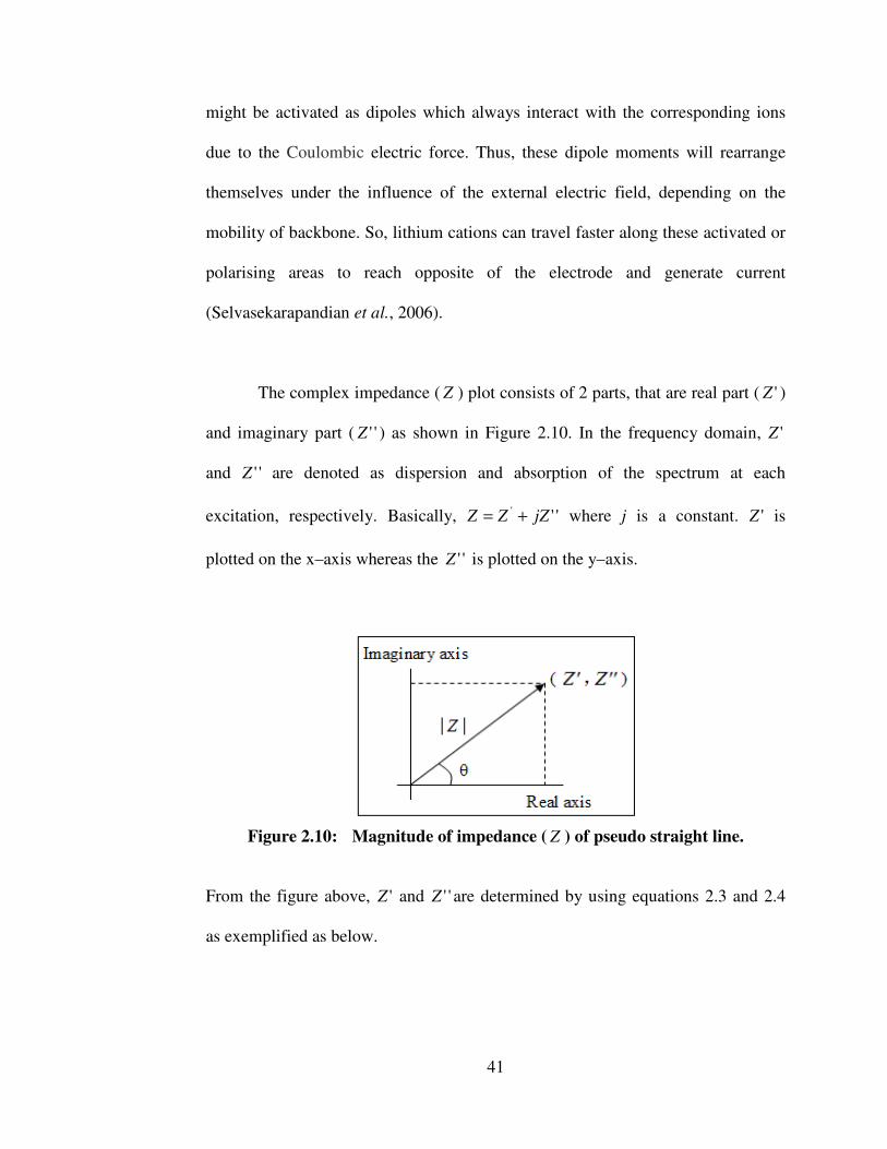
41
might be activated as dipoles which always interact with the corresponding ions
due to the Coulombic electric force. Thus, these dipole moments will rearrange
themselves under the influence of the external electric field, depending on the
mobility of backbone. So, lithium cations can travel faster along these activated or
polarising areas to reach opposite of the electrode and generate current
(Selvasekarapandian et al., 2006).
The complex impedance ( Z ) plot consists of 2 parts, that are real part ( 'Z )
and imaginary part ( ''Z ) as shown in Figure 2.10. In the frequency domain, 'Z
and ''Z are denoted as dispersion and absorption of the spectrum at each
excitation, respectively. Basically, ''' jZZZ += where j is a constant. 'Z is
plotted on the x–axis whereas the ''Z is plotted on the y–axis.
Figure 2.10: Magnitude of impedance ( Z ) of pseudo straight line.
From the figure above, 'Z and ''Z are determined by using equations 2.3 and 2.4
as exemplified as below.

42
Z' = | Z | cos �
Z'' = | Z | sin �
where � is the phase of impedance
However, there is a main shortcoming for the complex impedance. From the entire
data plot, the indication of frequency is absent. Therefore, it can be concluded that
low frequency data are located on the right side of the plot whereas the higher
frequency are on the left side (Rajendran et al., 2002).
2.8.2 Dielectric Study
Frequency dependence studies of the conductivity and of the dielectric
response are useful techniques to obtain the detailed information of ionic
conduction mechanism and differences in ion–polymer interactions in polymer
electrolytes (Gray, 1991c). Dielectric relaxation study is an approach to investigate
the dynamic and relaxation behavior of the electric dipoles in the polymer matrix
by studying the electrode polarization effect onto the polymer electrolytes (Gray,
1991c; Rajendran et al., 2004). Conductivity relaxation refers as a phenomenon
where the time is required to build up the charge carriers at the electrode–
electrolyte interface before the electric field changes the direction (Baskaran et al.,
2006a). The resulting in a net cumulative moment will give rise to a relaxation.
The build up of the charge carriers are known as polarization. The polarization
disappears when the voltage is removed (West, 1999a).
(Equation 2.3)
(Equation 2.4)

43
In general, there are three types of relaxation process in the dielectric study:
�’ relaxation, � relaxation and � relaxation. �’ relaxation depends on the molecular
weight and its amplitude is lower than others, ascribing to crystal–disordering
mechanism. In contrast, � relaxation is a relaxation in the amorphous phase which
emphasizes onto the relationship between the segmental mobility of polymer
chains and their strong Arrhenius behavior in temperature dependence study.
Empirical Vogel–Tamman–Fulcher (VTF) equation is mainly been used to explain
� relaxation by exhibiting a non-linear temperature dependence study. On the
contrary, � relaxation is related to the localized motions of the structural units and
it has a weaker Arrhenius–type behavior in temperature dependence study (or
linear relationship). It is associated with an amorphous transition involving short–
range bond rotations (Fernandez et al., 2008).
The real part of dielectric relaxation constant (also known as dielectric
constant, 'ε ) is the direct measure of stored charge in a material (Kumar and Bhat,
2009), whereas imaginary permittivity of the dielectric relaxation constant (also
known as dielectric loss) is a direct measure of dissipation of energy which
generated from transportation of charge carriers and polarization effect of charge
carriers (Stephan et al., 2000b). It is used to study the energetic of relaxations of
complex ionic defects (Barsoukov & Macdonald, 2005b). Polymer electrolytes
should possess high dielectric strength and low dielectric loss. It is because the low
dielectric constant will limit the reduction of the dimensions of the polymer
electrolytes. As a result, the existence of strong electric fields will alter and

44
degrade the device performance. On the other hand, high dielectric constant is able
to withstand high voltages without undergoing the degradation (West, 1999a).
2.8.3 Horizontal Attenuated Total Reflectance–Fourier Transform Infrared (HATR–FTIR) Spectroscopy
The main fundamental of FTIR is to determine structural information about
a molecule. FTIR brings greater versatility to polymer structural studies. It
facilitates the study of such polymer reactions as degradation or cross–linking
because the spectra can be scanned, recorded and transformed into a matter of
seconds. Besides, it is a qualitative identification of unknown sample. It is
accomplished by the comparison. In addition, it allows the spectra to generate the
hidden spectra via digital subtraction. A very small size is sufficient to undergo the
analysis for highly localized sections of the sample by coupling the FTIR
instrument with a microscope. FTIR is also used to study the polymer blends. If
the immiscible blend of polymers, the IR spectrum will exhibit a superposition of
two homopolymer spectra. Additionally, the interaction which arises from
chemical or physical interaction between the homopolymer is also exhibited
(Malcolm and Stevens, 1999b).
The main principle of FTIR is based on interferometry which is an optic
study. It separate infrared beam of light which serves as light source radiation into
two ray beam. Once the beam of infrared is passed through the sample, the
molecules absorb infrared radiation and then excited to a higher energy state. Thus,

45
the energies associated with these vibrations are quantized; within a molecule,
only specific vibrational energy levels are allowed. The amount of energy
absorbed at each wavelength was recorded. The frequencies which have been
absorbed by the sample are determined by detector and the signal is amplified.
Hence, IR spectrum was obtained. FTIR spectroscopy is not only applied in the
crystalline region of complexation, whereas the complexation in amorphous phase
can also be determined (Ramesh and Chai, 2007).
On the contrary, HATR is an internal reflection accessory which can
simplify the FTIR analysis of pastes, gels, semi–solids, powders and films. The
FTIR spectrum is easily to be collected via this horizontal sampling surface, with
minimal sample preparation, in all laboratory environments. HATR used to
analyze samples that are too strongly absorbing for conventional transmittance
measurements, because HATR is a surface–sampling technique. HATR is supplied
with a top plate fitted with a Zinc Selenide (ZnSe) crystal.
2.8.4 X–ray Diffraction (XRD)
XRD is used as fingerprint method to detect the presence of a known
compound or phase in a specimen. It is a useful method in the identification of
compounds for qualitative analysis. It is also widely been probed to provide a
rough check of the purity of sample (Smart and Moore, 2005b). It is an
identification of unknown crystalline materials, characterization of crystalline

46
material and determination of unit cell dimensions. In general, X–ray is an
electromagnetic radiation of wavelength ~1 Å (10-10m) and lies between �–ray and
the ultraviolet in the electromagnetic spectrum. A filament, usually tungsten, is
electrically heated and thus a beam of electrons are emitted. These electrons are
accelerated by a high potential difference (20–50kV) and thus allowed to strike a
metal target, often copper (Cu). The incident electrons have sufficient energy to
knock out (or ionize) electrons from the innermost K shell ( n =1) and this in turn
creates vacancies. An electron in an outer orbital (2p or 3p) immediately drops
down to occupy the vacant and the energy released appears as radiation, as shown
in Figure 2.11. The electrons descending from the L shell ( n =2 or 2p) produce K�
lines with a wavelength of 1.5418 Å, whereas the electrons from the M shell ( n =3
or 3 p) will give rise to K� lines with wavelength of 1.3922 Å. K� transition occurs
more frequently than K� transition. K� line is usually selected and K� line is filtered
out by using a filter made of nickel metal foil. In XRD, monochromatic radiation,
which defined as single wavelength or a very narrow range of wavelengths, is
required (West 1999b; Smart and Moore, 2005b).
Figure 2.11: Generation of K� and K� transitions.

47
Bragg’ s law is executed in powder diffraction technique. In this approach,
XRD behaves like “ reflection” from the planes of atoms within crystal and that
only at specific orientations of the crystal with respect to the source and detector
are X–rays “ reflected” from the planes. Figure 2.12 illustrates the Bragg condition
for the reflection of X–rays by a crystal. Two X–rays beams, Ray 1 and Ray 2, are
reflected from adjacent plans, where the spacing between the atomic planes occurs
over the distance, d. Ray 1 reflects off the upper atomic plane at an angle of
θ which equal to its incident angle. Similarly, Ray 2 reflects off the lower atomic
plane at the same angle θ. However, it has to travel the extra distance xyz (or
distance of 2a) as compared to Ray 1. For the reflected beams to emerge as a
single beam of reasonable intensity, they must reinforce, or arrive in phase with
one another. This phenomenon is known as constructive interference. For
constructive interference to take place, the path lengths of the interfering beams
must differ by an integral number of wavelengths (nλ). The perpendicular distance
between pairs of adjacent planes (d) and the angle of incidence, or Bragg angle (�)
are related to the distance xy by
xy = yz = d sin �
The difference in path length between the two beams is given by:
Difference in path length = xy + yz
Thus, difference in path length = 2d sin �
This must be equal to an integral number, n, of wavelengths. If the wavelength of
the X–rays is λ, then
nλ = 2d sin �
(Equation 2.5)
(Equation 2.6)
(Equation 2.7)

48
This is known as the Bragg equation. At angles of incidence other than Bragg
angle, the reflected beams are out of phase and destructive interference or
cancellation occurs (West 1999b; Smart and Moore, 2005b).
Figure 2.12: Derivation of Bragg’s law.
A finely ground crystalline specimen consists of abundant of small crystals,
which known as crystallites. These crystallites orient randomly to one another. The
sample is placed in the path of a monochromatic X–ray beam, the planes in these
crystallites will orient at the correct angle to fulfill the Bragg condition and hence
form the diffraction. The diffracted beams make an angle of 2� with the incident
beam. The collection of powder diffraction patterns is performed by automatic
diffractometers. A scintillation or CCD detector is used to record the angle and the
intensity of diffracted beams, which are plotted as intensity against 2� (Smart and
Moore, 2005b). The increase in the width of the diffraction peak indicates the
decrease in the crystallite size.

49
2.8.5 Scanning Electron Microscopy (SEM)
In the characterization of solid–state compound, scanning electron
microscopy (SEM) is widely used to investigate the structure, morphology and
crystallite size, to examine the surface defects of crystal, and to determine the
distribution of elements (Smart and Moore, 2005b). In this technique, an electron
beam is produced by heating the tungsten filament and then focused by magnetic
fields in a high vacuum. The vacuum prevents the interaction of the beam with any
extraneous particles in the atmosphere. The electrons from this finely focused
beam are scanned across the surface of a sample in a series of lines and frames
called a raster. At any given moment, the specimen is then bombarded with
electrons over a very small area. These electrons may be elastically reflected by
the surface of the sample with no loss of energy (backscattered electrons), they
may be absorbed and emitted secondary electrons of low energy, they may be
absorbed and give rise to the emission of visible light, and they may give rise to
electric currents within the specimen. All these effects can be detected and hence
given a map of the surface topography of samples (Braun, 2005c; Smart and
Moore, 2005b). Some of the samples may need to be coated with gold or graphite
to stop charge building up on the surface of the specimen (Smart and Moore,
2005b).
For backscattered electrons, the atomic number of the elements in the
sample is used to determine the contrast in the produced image. The image will
show the distribution of different chemical phases in the sample. The resolution in

50
the image is not as good as for secondary electrons because of the emission of
these electrons from a depth in the sample. Among all the means, the low–energy
secondary electron technique is the most common method. The primary electrons
enter a surface of the specimen with an energy of 0.5–30keV and generate many
low–energy secondary electrons. The intensity of these secondary electrons is
mainly governed by the surface topography of the sample. The image of the
sample can thus be constructed by measuring secondary electron intensity as a
function of the position of the scanning primary electron beam. High spatial
resolution can be obtained because the primary electron beam can be focused to a
very small spot (< 10nm).
2.8.6 Differential Scanning Calorimetry (DSC)
Thermal analysis is a technique to investigate the properties of solids as a
function of a change in temperature. In this work, the thermal analyses employed
are differential scanning calorimetry (DSC) and thermogravimetric analysis (TGA).
DSC is a quantitative study of thermal transitions of polymer matrix by heating
polymer sample and an inert reference. The reference is either an empty cup or a
cup containing an inert material, such as anhydrous alumina. In DSC, the
individual heaters are provided to the sample and reference. Then, the energy is
supplied to isothermal both of the samples and reference. Hence, the electrical
power difference between sample and reference (d�Q/dt) is measured. The data
are plotted as d�Q/dt on the coordinate against temperature on the abscissa and the

51
plots are known as thermograms. The major advantage of DSC is the peak areas of
thermograms are directly related to enthalpy changes in the sample. Therefore, the
data obtained can be used for measurements of heat capacities, heats of fusion and
enthalpies of reactions (Malcolm and Stevens, 1999b). In addition, DSC measures
the amount of heat released by a sample as the temperature is increased or
decreased at a controlled uniform rate (Smart and Moore, 2005b).
The basic principle of DSC depends on the amount of heat needed to flow
in to maintain the samples and reference at the same temperature when the samples
undergoes some physical transformation such as phase transition. Thus,
exothermic and endothermic reactions play a vital role. In general, endothermic
reaction is a process that absorbs energy in the form of heat, whereas for the
exothermic process, heat will be released. So, the endothermic process such as
melting process at which the matrix polymer electrolytes is melted to a liquid form
will require more heat flowing into the sample to increase its temperature at the
same rate as the reference. On the other hand, the heat required is lesser to raise
the temperature of sample if it undergoes an exothermic phase transition such as
crystallization from matrix polymer to liquid state. Therefore, both the sample and
reference are maintained nearly at the same temperature throughout the experiment.
In general, the temperature program for a DSC analysis is designed to ensure
temperature of the sample holder increases linearly as a function of time. In
conclusion, the DSC plays an important role to determine the glass transition
temperature ( gT ), crystallization temperature ( cT ) and crystalline melting point

52
( mT ). Other than that, the decomposition temperature ( dT ) can also be obtained as
well.
gT is a vital characteristic of the amorphous behavior of a polymer during
the transition from solid to liquid (or melt) state. The kinetic energy of the
molecules increases if an amorphous polymer is heated. As the polymer retains in
the glass–like properties, the mobility of molecules are still restricted even there is
a presence of short–range vibrations and rotations. As the temperature is further
increased or the polymer matrix is further melted, its glass–like structure will be
converted into rubbery state which is soft and elastomeric. This characteristic
temperature is known as gT . At this transition, it is accompanied by more long
range molecular motion and thus the degree of rotational freedom increases. As a
result, there is more segmental movement among the atoms of the chains. Thus,
the space between the atoms will be increased and then results in the increase of
the specific volume.
It is less commonly known as second–order transition temperature because
it is associated with a change in heat capacity but no latent heat is involved in this
process. It depends on the chemical nature of the polymer, on the configuration, on
the degree of crystallinity, on the length of the side chains, and on the degree of
branching (Braun, 2005c). There are two methods to determine gT . Firstly, the
temperature at which this change in specific volume takes place was determined
by dilatometry method. Another method to measure gT is called calorimerty. It is

53
based on the enthalpy change of the polymer at the glass transition. In contrast, the
modulus (also known as stiffness) decreases appreciably and it is readily detected
by using mechanical measurement.
After it reaches above gT , the molecules start to gain the freedom in
motion. Once they reached a particular stage where they have enough freedom of
motion, thus they will arrange themselves spontaneously into a crystalline form. At
this state, it is known as crystallization temperature ( cT ) and the heat is given out.
So, it is an exothermic reaction and it results a peak in the DSC thermograms as
shown in Figure 2.13. As the polymer is further heated, it will lose the elastometric
properties and it melts to a flowable liquid. At this point, the crystalline melting
temperature, mT is reached. In this transition, an endothermic process was
undergone. Transitions like crystallization and melting, which do have latent heats,
are called as first–order transitions. If the heating is continued, the polymer will be
degraded and it is known as decomposition temperature, dT (Malcolm, 1999b).

54
Figure 2.13: A schematic DSC thermogram demonstrating the appearance
of several common features, which are glass transition, crystallization and melting process.
2.8.7 Thermogravimetric Analysis (TGA)
TGA is a versatile thermal and primarily used to determine thermal
stability and thermal degradation of the samples as a function of change in
temperature under inert conditions. In general, the thermal stability is concerned
with chemical transformations. The main principle of TGA is to monitor the
weight of the samples on a sensitive balance (also known as thermobalance)
continuously as the sample temperature is increased under an inert atmosphere or
air at a controlled uniform rate. The data were recorded as a thermogram of weight
which is in y–axis against sample temperature which is in x–axis. In addition, the
TGA is used to characterize the polymer in a copolymer by monitoring the weight
loss of a known entity which correlated to percentage of the polymer into the
copolymer.
exo endo

55
Apart from that, it also used to determine the volatilities of plasticizers and
other additives (Malcolm and Stevens, 1999b). TGA does not only capable of
determining the weight loss or weight gain of a polymer after heated at high
temperature, it can also be used to determine the melting point ( mT ) and
decomposition temperature ( dT ). mT can be further confirmed with the result
obtained from the DSC. At low temperature, the weight loss may results from
evaporation of residual solvent and moisture, whereas the decomposition of
polymer is the contributor for the weight loss at high temperature. There are
several factors affect the TGA curve. The primary factors are heating rate and
sample size. Other features such as the particle size of the sample, its morphology,
and the gas flow rate can also affect the progress of thermal reaction (Braun,
2005c).
2.8.8 Rheological Studies
As usual, the ionic conductivity is closely related to the viscosity of sample.
For instances, low viscosity of sample will produce high ionic conductivity by
forming more voids within the polymer matrix. Therefore, the physical properties
of samples are also well been studied in order to understand the effect of physical
characteristics onto bulk ionic transportation further. In general, all materials can
behave as solid or liquid. Solid–like materials flow as liquids under a sustained
shear stress at very long time (or equivalently at very low frequency). It can

56
therefore be concluded that all materials are visco–elastic and it depends on the
timescale of deformation.
Rheology study is a well known physical technique to study the flow and
deformation properties of materials (Kavanagh and Murphy, 1998). It is composed
of two main tests that are rotational test and oscillation test. Rotational test is used
to determine to the flow behavior of sample after the stress was applied onto the
sample, whereas the viscoelastic behavior is explored by oscillation test. Examples
of rotational test are flow curve, viscosity curve and thixotropy which defined as
structure recovery. On the other hand, oscillation test are such as amplitude sweep
(AS), frequency sweep (FS) and temperature sweep (TS). Amplitude sweep is
probed to study the linear visco–elastic (LVE) range of the sample, whereas
frequency sweep is the oscillatory equivalent to the rotational flow curve which
scrutinizes the long–term structural stability of samples.
Amplitude sweep is designed to measure the visco–elastic properties of
samples without the disruption of the internal structures (Ebagninin et al., 2009). A
sinusoidal stress as a function of the angular frequency ( ω ) and the stress
amplitude ( 0τ ) is applied on the samples with its responding sinusoidal strain
(Durairaj et al., 2009). Both applied stress and resultant strain are expressed as
below:
( )tωττ sin0=
( )δωγγ += tsin0
(Equation 2.8)
(Equation 2.9)
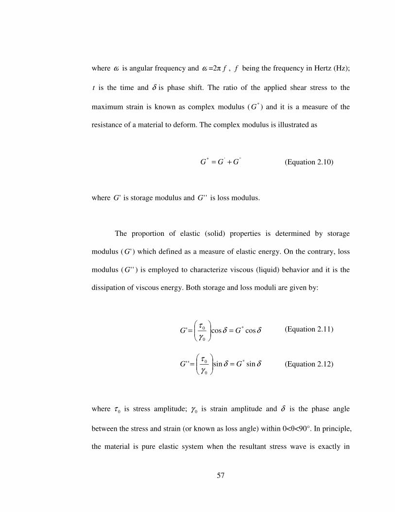
57
where ω is angular frequency and ω =2� f , f being the frequency in Hertz (Hz);
t is the time and δ is phase shift. The ratio of the applied shear stress to the
maximum strain is known as complex modulus ( *G ) and it is a measure of the
resistance of a material to deform. The complex modulus is illustrated as
"'* GGG +=
where 'G is storage modulus and ''G is loss modulus.
The proportion of elastic (solid) properties is determined by storage
modulus ( 'G ) which defined as a measure of elastic energy. On the contrary, loss
modulus ( ''G ) is employed to characterize viscous (liquid) behavior and it is the
dissipation of viscous energy. Both storage and loss moduli are given by:
δδγτ
coscos' *
0
0 GG =���
����
�=
δδγτ
sinsin'' *
0
0 GG =���
����
�=
where 0τ is stress amplitude; 0γ is strain amplitude and δ is the phase angle
between the stress and strain (or known as loss angle) within 0<�<90°. In principle,
the material is pure elastic system when the resultant stress wave is exactly in
(Equation 2.10)
(Equation 2.11)
(Equation 2.12)

58
phase with the strain, along with δ =0. On the other hand, when the rate of change
of sinusoidal oscillation is a maximum and the strain is becoming to zero, the
perfect viscous sample is described if the resultant stress wave is exactly �/2 (or
equivalent as 90°) out of phase with the imposed deformation (Kavanagh and
Murphy, 1998; Durairaj et al., 2009; Ebagninin, 2009).

59
CHAPTER 3
MATERIAL AND METHODS
3.1 Materials
The host polymers, PMMA with an average molecular weight of 350000
was obtained from Aldrich while high molecular weight of PVC was obtained
from Fluka. The inorganic dopant salt, LiTFSI and ionic liquid, BmImTFSI were
obtained from Fluka and Sigma–Aldrich, respectively. The nanocomposite
inorganic filler, SiO2 with the particle size 7 nm was obtained from Sigma–Aldrich
while the solvent, tetrahydrofuran (THF) AR. grade was obtained from J.T.Baker.
All materials were used without further purification. All the polymer blend
electrolytes were prepared by solution casting technique.
3.2 Preparation of Polymer Electrolyte
Prior to the preparation of the polymer electrolytes, LiTFSI was dried at
100 °C for 1 hour to eliminate trace amounts of water in the material. There are
four polymer blend electrolytes systems in this work, whereby first and second
systems are known as preliminary steps. The quantity of materials added was
expressed as weight percent (wt %). Appropriate amounts of materials were
dissolved in THF. The solution was then stirred continuously for 24 hours on a hot
plate (without heating) at room temperature to obtain a homogenous mixture of

60
polymer system at room temperature. After that, the solution was cast on a glass
Petri dish and allowed to evaporate slowly inside a fume hood.
3.2.1 First Polymer Blend Electrolytes System
First polymer blend electrolytes system was employed to figure out the
most compatible ratio of PMMA to PVC. Solid polymer electrolytes were formed
in this system. The compositions prepared were [xPMMA–(1–x)PVC] where x is
0.1, 0.2, 0.3, 0.4, 0.5, 0.6, 0.7, 0.8 and 0.9, with a fixed amount of LiTFSI. 10 wt%
of LiTFSI was fixed. The compositions of PMMA and PVC and their designations
were tabulated in table below.
Compositions of PMMA: PVC Designations PMMA (wt %) PVC (wt %)
PE 1 90 10 PE 2 80 20 PE 3 70 30 PE 4 60 40 PE 5 50 50 PE 6 40 60 PE 7 30 70 PE 8 20 80 PE 9 10 90
Table 3.1: Designations of first polymer blend electrolytes system.
3.2.2 Second Polymer Blend Electrolytes System

61
From first system, 70 wt% of PMMA and 30 wt% of PVC was achieved
the highest ionic conductivity. Thus, this ratio is being fixed in this system. In
contrast, the most compatible ratio of polymer blends PMMA–PVC to LiTFSI was
determined in second polymer blend electrolytes system. Similarly, solid polymer
electrolytes were formed. The quantity of LiTFSI salt added into the polymer
blends was ranged from 5 wt% to 50 wt%. The weight fractions of polymer blends
to LiTFSI and their designations are shown in Table 3.2.
Compositions of PMMA–PVC : LiTFSI Designations PMMA–PVC (wt %) LiTFSI (wt %)
SPE 1 95 5 SPE 2 90 10 SPE 3 85 15 SPE 4 80 20 SPE 5 75 25 SPE 6 70 30 SPE 7 65 35 SPE 8 60 40 SPE 9 55 45
SPE 10 50 50 Table 3.2: Designations of second polymer blend electrolytes system.
3.2.3 Third Polymer Blend Electrolytes System
BmImTFSI ionic liquid was further added in third polymer blend
electrolytes system, leading to formation of gel polymer electrolytes. The
BmImTFSI content dispersed in the polymer electrolytes lies within the range of
10 and 90 wt%. PMMA–PVC (70 wt%) and LiTFSI (30 wt%) were employed as

62
fixed variables as SPE 6 achieved the maximum ionic conductivity in previous
system. Table 3.3 shows the variation of the compositions of polymer blend
electrolytes (PMMA–PVC–LiTFSI) and ionic liquid and their designations.
Compositions of PMMA–PVC–LiTFSI : BmImTFSI Designations PMMA–PVC–LiTFSI (wt %) BmImTFSI (wt %)
IL 1 90 10 IL 2 80 20 IL 3 70 30 IL 4 60 40 IL 5 50 50 IL 6 40 60 IL 7 30 70 IL 8 20 80 IL 9 10 90
Table 3.3: Designations of third polymer blend electrolytes system.
3.2.4 Fourth Polymer Blend Electrolytes System
Since IL 6 exhibited the highest ionic conductivity, thus the ratio of 40
wt% of PMMA–PVC–LiTFSI to 60 wt% of BmImTFSI is fixed in this system.
Nanocomposite polymer electrolytes were formed in fourth system by dispersing
nano–sized SiO2. In this work, addition of 2, 4, 6, 8 and 10 wt % of SiO2 was
investigated and assigned as CPE 1, CPE 2, CPE 3, CPE 4 and CPE 5, respectively,
as tabulated as follow:

63
Compositions of PMMA–PVC–LiTFSI–BmImTFSI : SiO2 Designations PMMA–PVC–LiTFSI–BmImTFSI
(wt %) SiO2 (wt %)
CPE 1 98 2 CPE 2 96 4 CPE 3 94 6 CPE 4 92 8 CPE 5 90 10
Table 3.4: Designations of fourth polymer blend electrolytes system.
3.3 Characterizations of Polymer Electrolytes
3.3.1 Impedance Spectroscopy
The prepared samples were subjected to alternating current (AC)–
impedance spectroscopy for ionic conductivity studies. The thicknesses of the
polymer electrolytes were measured by using a micrometer screw gauge. The
parameter of thickness of the polymer electrolytes is very vital because the result
may be affected if there is any change of thickness. The measurement of thickness
should be repeated a few more times onto the surroundings of the samples in order
to obtain an average thickness. It aims to produce a more precise result. The ionic
conductivities of the samples were determined, by using HIOKI 3532–50 LCR
HiTESTER, over the frequency range of 50 Hz to 1 MHz. Two stainless steel (SS)
blocking electrodes were used in this study with the configuration SS/ PE/ SS.
64
3.3.1.1 Ambient Temperature–Ionic Conductivity and Temperature Dependence–Ionic Conductivity Studies
For ambient temperature–ionic conductivity, the ionic conductivities of the
samples were measured at room temperature. On the other hand, the measurements
of ionic conductivities of the polymer electrolytes were taken from ambient
temperature until 80 °C, for temperature dependence–ionic conductivity studies.
The bulk ionic conductivity of polymer electrolytes is determined by using the
equation below.
ARb
�=σ
where � is the thickness (cm); Rb is bulk resistance () and A is the known surface
area (cm2) of polymer electrolytes. The semicircle fitting was accomplished to
obtain Rb value. Rb of the thin electrolytes film was calculated from extrapolation
of the semicircular region on Z real axis ( 'Z ), as shown in Appendix A. Besides,
'Z and Z imaginary ( ''Z ) axis must be in equal scale because the radius of a
circle must be the same.
(Equation 3.1)

65
3.3.1.2 Frequency Dependence–Ionic Conductivity Studies
In this study, the conductivity was expressed as below:
AG�=σ
where G is the conductance (S) which obtained from impedance spectrometer by
choosing this parameter.
3.3.1.3 Dielectric Behavior Studies
The complex dielectric behavior of a polymer electrolyte system was
expressed as:
''' εεε i+=∗
( ) ( )22* "' εεε +=
where 'ε and ''ε are real and imaginary parts of dielectric constant of the polymer
electrolyte system. On the contrary, these 'ε and ''ε of the dielectric constants
were determined as follows:
A
C
o
p
εε
�='
(Equation 3.2)
(Equation 3.3)
(Equation 3.4)
(Equation 3.5)

66
oωεσε =''
where pC is parallel equivalent static capacitance which obtained from impedance
spectrometer by choosing this parameter; oε is permittivity in free space (also
known as electric constant) which is equal to 8.856 × 10⁻¹⁴ Fcm-1; ω is angular
frequency and ω =2� f , f being the frequency in Hertz (Hz).
3.3.1.4 Dielectric Moduli Formalism Studies
The complex dielectric modulus can be determined by the equation below:
''' iMMM +=∗
( ) ( )22* "' MMM +=
where *M is the complex dielectric modulus; 'M is real part of dielectric
modulus and ''M is imaginary part of dielectric modulus. In contrast, 'M and ''M
are expressed as below:
])()[(' 2''2'
'
εεε+
=M
])()[('' 2''2'
''
εεε+
=M
(Equation 3.6)
(Equation 3.7)
(Equation 3.8)
(Equation 3.9)
(Equation 3.10)

67
3.3.2 Horizontal Attenuated Total Reflectance–Fourier Transform Infrared (HATR–FTIR)
HATR–FTIR analysis was carried out by using FTIR Spectrometer
Spectrum RX1 (Perkin–Elmer) with HATR, an internal reflection accessory, in the
wave region between 4000 cm-1 and 650 cm-1. The resolution of the spectra
obtained at room temperature was 4 cm-1 and recorded in the transmittance mode.
3.3.3 X–ray Diffraction (XRD)
The amorphous degree of polymer electrolytes was investigated using
XRD. The XRD patterns were recorded on a Siemens D 5000 diffractometer with
Cu–K� radiation (=1.54060 Å), over the range of 2�=5–80° at ambient
temperature. Debye–Scherrer equation is used to determine the coherence length
as shown as below:
bb
Lθθ
λcos29.0
∆=
where is X–ray wavelength; bθ is glancing angle of the peak; bθ2∆ is full
width at half maximum (FWHM). The peak at 2�≈ 18° was chosen to determine
the coherence length for the polymer electrolytes.
3.3.4 Scanning Electron Microscopy (SEM)
(Equation 3.11)

68
Using Leica’ s SEM (model S440) at 10kV, the morphology of polymer
blends at room temperature was studied. Insulators such as pure PMMA, pure
PVC and PMMA–PVC samples were coated with a thin layer of gold to prevent
electrostatic charging.
3.3.5 Differential Scanning Calorimetry (DSC)
DSC analysis was carried out, under nitrogen flow rate of 50 ml min-1,
using a METTLER TOLEDO Thermal Analyzer which comprised of DSC 823e as
the main unit and STARe software. Samples weighing approximately 2–3 mg were
hermetically sealed in a 40�l aluminum crucible and then perforated in order to
keep the samples at atmospheric pressure. The samples were heated from 25°C to
105°C to remove any traces of solvent and water. The temperature was then
maintained at 105°C for 2 minutes to ensure the complete evaporation. The
samples were then cooled rapidly to 25 °C and then reheated to 450°C at a heating
rate of 10°C min-1. The final heating scan was used to evaluate the gT , mT and dT .
The mid point of endothermic reaction is assigned as gT . The endothermic peak
point of melting and decomposition are assigned as mT and dT , respectively.
3.3.6 Thermogravimetric Analysis (TGA)

69
TGA was carried out using a METTLER TOLEDO Thermal Gravimetric
Analyser which comprised of TGA/SDTA851e as the main unit and STARe
software. Samples weighing 2–3 mg were placed in a 150�l silica crucible. The
samples were then heated from 30°C to 400°C, at a heating rate of 10°C min-1,
under nitrogen flow rate of 10 ml min-1.
3.3.7 Rheological Studies
Rheological measurements were performed on Anton–Paar Physica MCR
301 rheometer. The geometry was a cone plate with diameter of 60mm and gap
height of 0.056mm. All the rheological measurements were carried out at ambient
temperature with fresh sample. All the parameters were in logarithm scale. The
sample was sandwiched between stainless steel cone plate geometry and a
stationary bottom plate and excessive sample is trimmed thereafter. Solvent trap
was used to slow down the evaporation process of solvent in the sample. Before
starting the test, about 1 min of rest period was allowed, in order to stabilize the
normal forces between the polymer electrolytes and the cone plate.
3.3.7.1 Amplitude Sweep and Oscillatory Stress Sweep

70
Amplitude and oscillatory stress sweeps studies were examined in a log
strain ramp from 0.001 % to 150 % with 5 points per decade at angular frequency
of 10s-1. For time setting, 30 measuring points with 5 seconds duration had been
set in the whole measurement.
3.3.7.2 Oscillatory Frequency Sweep
All the data acquisitions for frequency sweep tests were carried out over a
frequency range between 0.01s-1 and 0.1s-1, with 20 measuring points per 5
seconds duration.
3.3.7.3 Viscosity Test
As the profile of viscosity curves, a fixed shear rate parameter, ranging
from 0.1s-1 to 100s-1, with 32 measuring points per 5 seconds duration were
recorded.

71
CHAPTER 4
RESULTS AND DISCUSSION OF FIRST POLYMER BLEND
ELECTROLYTES SYSTEM
4.1 AC–Impedance Studies
Figure 4.1 shows the typical impedance plot for PE 3 at room temperature.
In general, this impedance plot has been divided into two well defined regions: a
slanted spike at low frequency and a semicircle portion which reveals the
characteristic of a parallel combination of bR and bulk capacitance of the polymer
matrix at high frequency (Venkateswarlu et al., 2000). However, the spike is
slanted at an angle less than 90°. This phenomenon indicates the non–idealism of
capacitance and induces to an establishment of double layer at the blocking
electrodes or also known as non–Debye effect. It implies that a constant phase
element is appeared at the electrode and polymer electrolyte interface and leads to
a formation of double layer at the electrodes. In addition, the angle and the amount
of inclination is attributed to the distribution of conductivity relaxation time which
defined as the time required to build up charges at the electrode and electrolyte
interface before the electric field changes the direction (Baskaran et al., 2006a).

72
Figure 4.1: Typical Cole–Cole plot for PE 3 at ambient temperature.
4.2 Ambient Temperature–Ionic Conductivity Studies
Figure 4.2 depicts the ionic conductivity of the polymer matrix with
different PVC content at ambient temperature. The ionic conductivity of polymer
matrix increases with PVC concentration, to an optimum level and then decreases.
Initially, the increase in ionic conductivity is due to the long range coulombic
forces leading to re–dissociation of solvated ion pairs. Then, more and more
number of free mobile charges is produced and these mobile charges are available
for segmental transportation in electrolytic conduction. Since the degree of
segmental mobility of charge carriers is increased, thus the ionic conductivity is

73
increased (Fu et al., 2003). After 30 wt% of PVC is blended into the system, it
exhibits the highest ionic conductivity of (1.60±0.08) × 10-8 Scm-1as shown in
Figure 1. This is because the mobility and concentration of mobile charge has
reached an optimum level and induces to this optimum ionic conductivity (Fu et
al., 2003). Another perception of having the highest ionic conductivity is that the
polymer electrolyte had reached the optimum percolation threshold where the
formation of percolation pathway will give rise to conductivity behavior of lithium
salt in the PE 3 to achieve the maximum limit (Ramesh and Chai, 2007).
As expected, the conductivity decreases as the amount of PVC is increased.
It is due to the formation of PVC–rich phase which is a solid–like medium and
leads to a hurdle for ion penetration in the electrolytic system. So, the ion must
transport via indirect movement along a convoluted pathway restricted to PMMA–
rich phase because of such blocking of transport of charges. Therefore, the ionic
conductivity of the polymer matrix is decreased (Rajendran et al., 2000).
Moreover, at the higher concentration of PVC, the re–dissociation of solvated ion
pairs is replaced with short range ion–solvent interaction. Although the number of
ions dissolved into the polymer matrix increases, the effective number of mobile
charges which are available for migration is reduced (Stephan et al., 2002)

74
-10.5
-10.25
-10
-9.75
-9.5
-9.25
-9
-8.75
-8.5
-8.25
-8
-7.75
-7.5
0 10 20 30 40 50 60 70 80 90 100
Percentage of PVC (wt %)
Log
con
duct
ivity
, log
[� (
Scm-1
)]
Figure 4.2: Variation of log conductivity, log � as a function of weight
percentage PVC added into PMMA–PVC–LiTFSI based polymer electrolyte at ambient temperature.
4.3 Temperature Dependence–Ionic Conductivity Studies
Figure 4.3 depicts the Arrhenius plot of PE 3, PE 5 and PE 9 which shows
that the ionic conductivity increases with temperature. This is attributed to the
expansion of polymer matrix. The polymer matrix expands with increase in
temperature and then weakens the interaction within the polymer matrix,
promoting the decoupling of Li cations from the polymer complex. This assists the
mobility of ions. The polymeric chain also acquires faster internal vibrational
modes with increasing the temperature, which in turn to increase in mobility of
polymer segments by initiating the bond rotation within the polymer matrix.
Therefore, it favors the ionic transportation and hence increases the ionic

75
conductivity (Baskaran, 2006b).
As shown in Figure 4.3, the regression values are close to unity, indicating
the presence of Arrhenius behavior. In this rule, the conductivity is expressed as:
��
���
� −=
kTE
A aexpσ
where A is a constant which is proportional to the amount of charge carriers, aE is
activation energy and k is Boltzmann constant, that is 8.6173×10⁻⁵ eV K-1 and T
represents the absolute temperature in K. In general, this theory follows the
hopping mechanism which states that the interaction of polar group of the
polymeric chain with Li+ is weaker and hence these charge carriers are decoupled
from the segmental motion of polymer matrix. This creates vacant sites in the
polymer chain. Therefore, the ions from adjacent sites tend to occupy these
neighboring vacant sites and form the coordination with the polymer chain.
Figure 4.3 shows that ionic conductivity of PE 3 is greater than PE 5 and
that of PE 5 is greater than PE 9. The amorphous nature of PE 3 increases as the
content of PMMA increases in comparison with PE 5 and PE 9. The increase in
amorphous region leads to the disorder mode of segmental polymer chain and thus
forms more free voids for ionic conduction. This promotes the ion transportation
and hence the increase in ionic conductivity (Achari et al., 2007). The lower ionic
conductivity of the polymer electrolyte is attributed to excessive cross–linking
(Equation 4.1)

76
effect. Higher amount of PVC incorporated in the polymer electrolytes leads to
high degree of cross–linking between PMMA and PVC and increases the viscosity
by forming entanglements within the polymer chain. As a result, free space for ion
transportation is reduced and then impedes the mobility of charge carriers.
Consequently, the ionic conductivity is decreased (Kumar et al., 2007). The
mechanism of cross–linking is discussed further in section 4.10.
The activation energy, aE , is also determined in this study. As discussed
earlier, the Li+ tends to dissociate from the polymer chain and other Li+ ions from
the surrounding favor to coordinate with the polymer chain with the aid of
segmental motion of polymer chain. Energy is required to overcome this
reorganization and reformation of the polymer chain with Li+. This energy is
defined as activation energy. As shown in Table 4.1, aE is inversely proportional
to ionic conductivity. This is mainly attributed to the amorphous region in the
polymer matrix, which is the prerequisite of the higher ionic conductivity. The
degree of amorphous phase leads to the disorderly arrangement of molecules in the
polymer matrix which results in a more flexible polymer chain. Therefore, the
attractive bonds between the macromolecules become weaker and requiring less
energy to break the bond for reorganization and reformation of coordination with
Li+. This enhances the Li+ diffusivity in the polymer matrix (Kumar et al., 2007).
Based on the above discussion it can be concluded that the hopping process is
favorable with decreasing aE .

77
-10.5
-10
-9.5
-9
-8.5
-8
-7.5
-7
2.8 2.9 3 3.1 3.2 3.3 3.4
1000/T(K-1)
Log
[ �
(Scm
-1)]
PE 3 PE 5 PE 9
Figure 4.3: Arrhenius plot of ionic conductivity of PE 3, PE 5 and PE 9.
Composition of PMMA and PVC (% wt)
PMMA PVC
Designations Activation energy, aE (eV)
70 30 PE 3 ��������
50 50 PE 5 ���� � �� �
10 90 PE 9 ���� �
Table 4.1: Activation energies for polymer blend electrolytes as a function of PVC loadings.
4.4 Frequency Dependence–Ionic Conductivity Studies
In order to understand the relaxation behavior of the polymer electrolytes
system, the ionic conductivity as a function of frequency for polymer electrolytes
is studied. The variation plot of logarithm of ionic conductivity with corresponding
frequency for PE 3 and PE 4 at ambient temperature is shown in Figure 4.4.

78
According to this figure, the ionic conductivity increases as the frequency is
increased. The low frequency dispersion region is attributed to interfacial
impedance or space charge polarization. As the frequency decreases, the amount of
charge accumulates at the electrode and electrolyte interface increases. As a
consequence, the number of mobile ions or charge carriers available for
transportation decreases and this leads to a decrease in ionic conductivity. This
indicates the presence of non–Debye properties in the polymer electrolytes. In
contrast, at higher frequency, the mobility of charge carriers is increased and
eventually contributes to higher ionic conductivity with respect to frequency
(Ramesh and Arof, 2001a).
-10
-9.5
-9
-8.5
-8
-7.5
-7
-6.5
1 1.5 2 2.5 3 3.5 4 4.5 5 5.5 6 6.5Log [f(Hz)]
Log
[�(S
cm-1
)]
PE 3 PE 4
Figure 4.4: Frequency–dependent conductivity at ambient temperature for PE 3 and PE 4.

79
4.5 Dielectric Relaxation Studies
The dielectric relaxation study is a versatile study used to investigate the
behaviour of polymer blends by studying the relaxation behaviour of dipoles of
polymer electrolyte (Rajedran et al., 2004). In this study, the same frequency range
is used for both PE 3 and PE 4 samples. Figures 4.5 and 4.6 illustrate the
frequency dependence variation of real ( 'ε ) and imaginary permittivity ( ''ε ) of
the dielectric relaxation constant for PE 3 and PE 4 polymers electrolytes
respectively. As shown in both figures, PE 3 prevails at higher region and this
indicates that PE 3 has higher mobile charge carriers for migration compared to PE
4. This eventually contributes to higher ionic conductivity and it has been proven
in Figure 4.2.
At low frequency, both real and imaginary parts of dielectric relaxation
constants rise sharply. This may be attributed to the electrode polarization effect
which may be due to the accumulation of charge at the electrode and electrolyte
interface and space charge effects which can normally be observed in ionic glasses.
This had further confirmed the presence of non–Debye characteristic in the
polymer matrix. In addition, it may also be due to the retention of trace amount of
water in the thin film (Goodwin et al., 1999). At high frequency, the decreases of
'ε and ''ε are mainly attributed to the high occurrence of periodic reversal of the
electric field at the interface which reduces the contribution of charge carriers. As
a result, it induces the absence of excessive ion diffusion in the direction of the

80
electric field (Ramesh and Chai, 2007). Thus, the orientation of the dipoles is
inhibited, resulting in a decrease in polarization. Since the interaction between
dipoles and external electrical field is becoming weaker, hence the values of 'ε
and ''ε decrease (Ramesh and Ng, 2009).
00.020.040.060.08
0.10.120.140.160.18
0.20.22
1 1.5 2 2.5 3 3.5 4 4.5 5 5.5 6 6.5Log [f(Hz)]
�'
PE 3 PE 4
Figure 4.5: Variation of real part of dielectric constant, 'ε with respect to frequency for PE 3 and PE 4 at ambient temperature.

81
0
0.5
1
1.5
2
2.5
3
3.5
1 1.5 2 2.5 3 3.5 4 4.5 5 5.5 6 6.5Log [f(Hz)]
�''
PE 3 PE 4
Figure 4.6: Variation of imaginary part of dielectric constant, ''ε with respect to frequency for PE 3 and PE 4 at ambient temperature.
4.6 Dielectric Moduli Studies
The dielectric moduli analysis is a further study to investigate the dielectric
behaviour of polymer blends by suppressing the polarization effects of the
electrode (Ramesh and Arof, 2001a). The real ( 'M ) and imaginary ( ''M ) parts of
dielectric moduli as a function of frequency for sample PE 3 and PE 4 are
exemplified in Figures 4.7 and 4.8, respectively. In these figures, the appearance of
the peaks in the modulus formalism at high frequency reveals that the polymer
electrolytes are ionic conductors. It may be due to the existence of bulk effect
(Ramesh and Chai, 2007). As shown in Figure 4.7, well–defined dispersion peaks
are absent, however, 'M is still showing a distinctive increment at high frequency.

82
The intensity of the peaks decreases as the PVC content increases. This implies
that there is a plurality of relaxation mechanism. On the other hand, the value of
'M and ''M tends to approach to zero at low frequency. This reveals that the
contribution of electrode polarization due to the accumulation of charge is
insignificant. Apart from that, for PE 3, the presence of long tail at low frequency
indicates the association of large capacitance with the electrodes (Ramesh and
Arof, 2001a).
0
10
20
30
40
50
60
70
80
90
1 1.5 2 2.5 3 3.5 4 4.5 5 5.5 6 6.5Log [f(Hz)]
M'
PE 3 PE 4
Figure 4.7: Variation of real part of modulus, 'M with respect to frequency for PE 3 and PE 4 at ambient temperature.

83
0
2
4
6
8
10
12
14
16
1 1.5 2 2.5 3 3.5 4 4.5 5 5.5 6 6.5Log [f(Hz)]
M''
PE 3 PE 4
Figure 4.8: Variation of imaginary part of modulus, ''M with respect to frequency for PE 3 and PE 4 at ambient temperature.
4.7 HATR–FTIR studies
The HATR–FTIR spectra of pure PMMA, pure PVC and PMMA–PVC are
shown in Figure 4.9 (a)–(c). The combination of HATR–FTIR spectra of pure
PMMA, pure PVC and PMMA–PVC is shown in Figure 4.10, whereas all the
assignments of the vibrational modes are tabulated in Table 4.2. As shown in
Figure 4.10, four peaks are disappeared upon addition of pure PVC into pure
PMMA compound. These peaks are assigned as trans C–H wagging mode of PVC
at 956 cm-1, CH2 deformation mode of PVC at 1328 cm-1, C–CH3 stretching mode
of PMMA at 1385 cm-1 and CH2 scissoring mode of PMMA at 1484 cm-1, as
highlighted in Figure 4.10. These disappearances indicate formation of

84
complexation between PMMA and PVC. All the characteristic peaks of (PMMA–
PVC) exhibit changes in shift, as listed in Table 4.2.
Figure 4.9 (a): HATR–FTIR spectrum of pure PMMA.
Figure 4.9 (b): HATR–FTIR spectrum of pure PVC.

85
Figure 4.9 (c): HATR–FTIR spectrum of PMMA–PVC.
Figure 4.10: Combination of HATR–FTIR spectra of (a) pure PMMA, (b)
pure PVC and (c) PMMA–PVC.

86
Wavenumber (cm-1) Description vibration modes PMMA
–PVC PMMA /
PVC Cis C–H wagging mode of PVC 698 691 CH2 rocking mode of PMMA 751 748 C–Cl stretching mode of PVC 842 834 Combination of C–O symmetric stretching mode in C–O–C linkage of PMMA and trans C–H wagging mode of PVC
963 966 / 956
CH2 wagging mode of PMMA 983 984 C–H rocking mode of PVC 1062 1063 C–O asymmetric stretching mode in C–O–C linkage of PMMA
1145 1141
CH2 twisting mode of PMMA 1193 1186 CH3 symmetric bending mode of PMMA 1244 1238 C–O–C symmetric stretching mode of PMMA 1269 1266 Combination of CH3 asymmetric bending mode of PMMA and C–H stretching mode of CH2 group of PVC
1436 1433 / 1425
C=C stretching mode of PVC 1684 1656 C=O stretching mode of PMMA 1725 1722 CH3 asymmetric stretching mode of PMMA and PVC 2941 2947 /
2911 Table 4.2: Assignments of vibrational modes of PMMA and PVC in
PMMA–PVC polymer blends.
As shown in Figure 4.11, pure PVC shows a sharp peak at 691 cm-1 and it
is assigned as cis C–H wagging mode of PVC. The characteristic peak is shifted to
698 cm-1 by blending with PMMA. On the other hand, the intensity of this
characteristic peak reduces from 8.70 % to 0.42 %, in transmittance mode. Upon
dispersion of PVC, CH3 asymmetric stretching mode of pure PMMA at 2947 cm-1
is shifted to 2941 cm-1. In term of intensity, the peak becomes broader due to the
interaction between PMMA and PVC, leading to an overlapping of CH3
asymmetric stretching mode of PMMA and PVC.

87
Figure 4.11: The comparison of change in intensity and shift of cis C–H
wagging mode of PVC in (a) pure PVC and (b) PMMA–PVC in the HATR–FTIR spectrum.
Apart from the changes in shift, it also demonstrates the change in shape.
As shown in Figure 4.12, two weak peaks are changed to a new weak peak with a
shoulder. Two apparent peaks are observed in the region of 1000–900 cm-1. For
pure PMMA, the first peak is designated as combination of C–O symmetric
stretching mode in C–O–C linkage of PMMA and trans C–H wagging mode of
PVC at 966 cm-1, whereas CH2 wagging mode of PMMA is assigned for second
peak at 984 cm-1. The first peak is shifted to 963 cm-1 due to the overlapping of
trans C–H wagging mode of PVC with C–O symmetric stretching mode of PMMA

88
by adding PVC. This indicates that PMMA is complexed with PVC. On the
contrary, the latter weak peak is changed to a shoulder peak and shifted to 983 cm-
1 by blending with PVC. This is further proven the interaction between PMMA
and PVC.
For pure PMMA, the C=O stretching mode of PMMA appears as a sharp
peak at 1722 cm-1. However, upon addition of PVC, a new sharp peak at 1725 cm-1
with a shoulder at 1684 cm-1 is obtained. This shoulder peak is assigned as C=C
stretching mode of PVC, revealing the entanglement of PMMA and PVC. Based
on the changes in shift, changes in intensity, changes in shape and disappearance
of the characteristic peaks, it can be concluded that there is a complexation
between PMMA and PVC in the PMMA–PVC polymer system.
Figure 4.12: The comparison of change in shape of the characteristic peaks within the region of 1000–900 cm-1 in (a) pure PMMA and (b) PMMA–PVC.

89
HATR–FTIR spectrum for pure LiTFSI, PE 3, PE 5 and PE 9 are
illustrated in Figures 4.13 (a)–(d), whereas Figure 4.14 shows the combination of
the HATR–FTIR spectrum. Table 4.3 depicts the assignments of important bands
of PE 3. Since PE 3 achieves the maximum ionic conductivity, thus the HATR–
FTIR spectrum of PE 3 is discussed in details. Seven new peaks are formed upon
addition of 10 wt% of LiTFSI as highlighted in Figure 4.14. These characteristic
peaks are assigned as trans C–H wagging mode of PVC at 923 cm-1, S–N–S
asymmetric bonding mode of LiTFSI at 1055 cm-1, C–SO2–N bonding mode of
LiTFSI at 1333 cm-1, SO2 asymmetric stretching mode of LiTFSI at 1357 cm-1,
CH3 asymmetric stretching mode of PMMA at 1963 cm-1 and S–CH3 bonding
mode of LiTFSI at 2827 cm-1 and 2996 cm-1. This is suggestive of the formation of
complexation between LiTFSI and PMMA–PVC blends.
The disappearance of some characteristics peaks is another way to prove
the interactions between LiTFSI and PMMA–PVC blends. For example, a weak
peak at 698 cm-1 is shown in Figure 4.9 (c). This peak is assigned as cis C–H
wagging mode of PVC. However, the peak is disappeared by adding 10 wt% of
LiTFSI. In comparing pure LiTFSI spectrum with PE 3 spectrum, it also found out
that the peak at 787 cm-1 which assigned as combination of C–S and S–N
stretching mode of LiTFSI is absent. The same phenomenon is also observed for
PMMA. Combination of C–O symmetric stretching mode in C–O–C linkage of
PMMA and trans C–H wagging mode of PVC which located at 963 cm-1 is also
disappeared, by comparing PMMA–PVC spectrum and PE 3 spectrum. These

90
absences of the characteristic peak divulge the formation of coordination bonding
between PMMA, PVC and LiTFSI.
Figure 4.13 (a): HATR–FTIR spectrum of pure LiTFSI.
Figure 4.13 (b): HATR–FTIR spectrum of PE 3.

91
Figure 4.13 (c): HATR–FTIR spectrum of PE 5.
Figure 4.13 (d): HATR–FTIR spectrum of PE 9.

92
Figure 4.14: Combination of HATR–FTIR spectra of (a) PMMA–PVC, (b)
pure LiTFSI, (c) PE 3, (d) PE 5 and (e) PE 9.

93
Wavenumber (cm-1) Description vibration modes PE 3 PMMA–PVC
/ LiTFSI Combination of CH2 rocking mode of PMMA and S–N stretching of LiTFSI
750 751 / 740
C–Cl stretching mode of PVC 895 842 Combination of C–O symmetric stretching mode in C–O–C linkage of PMMA and trans C–H wagging mode of PVC
923 963
CH2 wagging mode of PMMA 987 983 S–N–S asymmetric bonding mode of LiTFSI 1055 1065 C–H rocking mode of PVC 1085 1062 Combination of C–O asymmetric stretching mode in C–O–C linkage of PMMA and C–SO2–N bonding mode of LiTFSI
1150 1145 / 1147
Combination of CH2 twisting mode of PMMA and CF3 symmetric stretching mode of LiTFSI
1191 1193 / 1194
CH3 symmetric bending mode of PMMA 1241 1244 C–O–C symmetric stretching mode of PMMA 1269 1269 C–SO2–N bonding mode of LiTFSI 1335 1333 SO2 asymmetric stretching mode of LiTFSI 1364 1357 Combination of CH3 asymmetric bending mode of PMMA and C–H stretching mode of CH2 group of PVC
1460 1436
C=C stretching mode of PVC 1651 1684 C=O stretching mode of PMMA 1734 1725 CH3 asymmetric stretching mode of PMMA 1963 – S–CH3 bonding mode of LiTFSI 2827,
2996 2876, 2979
CH3 asymmetric stretching mode of PMMA and PVC 2900 2941 Table 4.3: Assignments of vibrational modes of PMMA, PVC and LiTFSI
in PE 3 polymer blend electrolyte.
All the characteristic peaks undergo the changes in shift; except the
characteristic peak at 1269 cm-1. The peak is assigned as C–O–C symmetric
stretching mode of PMMA and appeared as a shoulder peak. In order to probe the
complexation of PMMA, PVC and LiTFSI, the changes in intensity of
characteristic peaks are observed. At 750 cm-1, the weak peak is designated as
combination of CH2 rocking mode of PMMA and S–N stretching of LiTFSI. For

94
this characteristic peak, the intensity increases from 0.27 % to 0.5 %, in
transmittance mode. It may be due to the overlapping of S–N stretching of LiTFSI
with the rocking mode. As shown in Figure 4.15, in term of intensity, C=O
stretching mode of PMMA at 1734 cm-1 increases from 1.90 % to 2.60 %, in
transmittance mode. In addition, it exhibits upward shift, from 1725 cm-1 to 1734
cm-1. As can be seen, there is a visible change in shape in this figure. For PMMA–
PVC, the shoulder peak at 1684 cm-1 is assigned as C=C stretching mode of PVC.
In contrast, for PE 3, it has been changed to a new peak and shifted to 1651 cm-1,
as depicted in Figure 4.15.
Figure 4.15: The comparison of change in intensity of C=O stretching mode
of PMMA in (a) PMMA–PVC and (b) PE 3.

95
Another evidence to prove the change in shape is shown in Figure 4.16. For
PMMA–PVC polymer blends, the vibrational mode of CH3 asymmetric stretching
mode of PMMA and PVC shows a weak peak at 2941 cm-1 in the region of 3000–
2800 cm-1. However, three peaks are observed in this region upon dispersion of 10
wt% of LiTFSI. CH3 asymmetric stretching mode of PMMA and PVC shifts
downward to 2900 cm-1, whereas two new peaks are observed at 2827 cm-1 and
2996 cm-1. These peaks are assigned as S–CH3 bonding mode of LiTFSI. This
reveals the interaction between LiTFSI and PMMA–PVC polymer blends and
produces the complexation between lithium conducting salt and polymer blends in
the polymer electrolyte system. In addition, a weak peak is observed at 842 cm-1
and assigned as C–Cl stretching mode of PVC in PMMA–PVC. However, two
medium peaks are obtained by dispersing 10 wt% of LiTFSI in PE 3. As the first
peak, C–Cl stretching of PVC is observed at 895 cm-1, whereas combination of C–
O symmetric stretching mode in C–O–C linkage of PMMA and trans C–H
wagging mode of PVC at 923 cm-1 is designated for latter peak.
Figure 4.16: The comparison of change in shape of the characteristic peaks
in (a) PMMA–PVC and (b) PE 3 within the range of 3000–2800cm-1.

96
Some of the characteristic peaks are disappeared with increasing PVC
content. For both PE 5 and PE 9, CH3 asymmetric stretching mode of PMMA and
C=C stretching mode of PVC at 1651 cm-1 and 1963 cm-1, respectively, are absent
in comparison to PE 3. In addition, in the region of 3000–2800 cm-1, three weak
peaks are changed to two weak peaks for PE 5, revealing the absence of S–CH3
bonding mode of LiTFSI. On the contrary, for PE 9, there is only a weak peak
remains in this region. It further indicates the disappearance of both S–CH3
bonding modes of LiTFSI. Based on the absence of the characteristic peaks of
LiTFSI, this suggests that PVC particles favor to form agglomeration in the
polymer matrix rather than form complexation with LiTFSI. For PE 9, the peak
which assigned as trans C–H wagging mode of PVC is also disappeared upon
addition of PVC.
4.8 XRD studies
Figures 4.17 and 4.18 illustrate the XRD diffractograms of pure PMMA,
pure PVC, PMMA–PVC, pure LiTFSI and PMMA–PVC blend–based polymer
electrolytes. From Figure 4.17 (a), a broad characteristic peak of PMMA was
obtained at angles of 2�=16.4° with a shoulder at 2�=22.5° which reveals the
amorphous phase of PMMA. The intensity of these characteristic peaks is
decreased after the impregnation of PVC. This implies that the addition of PVC
disrupted the arrangement in the polymer backbone of PMMA (Baskaran et al.,
2006b). The presence of interactions between PMMA and PVC, such as cross–

97
linking, is attributed to this phenomenon. Complexation of PMMA and PVC
occurs with the aid of these interactions and it is further discussed in section 4.10.
Apart from the peak intensity of these characteristic peaks, another evidence of
complexation is observed. The blending of PMMA with PVC shifts the peaks at
2�= 16.4° and 2�= 22.5° to 15.8° and 22.3°, revealing the change in
crystallographic organization (Kumar et al., 2007).
Figure 4.18 (a) illustrates the sharp intense peaks at 2�=13.6°, 15.9°, 18.6°,
18.9° and 21.4° and reveals the crystalline character of LiTFSI. These crystalline
peaks were disappeared in PMMA–PVC based polymer blend electrolytes. The
absence of excess salt indicates that LiTFSI is fully complexed with PMMA and
PVC (Rajendran et al., 2004). A complete dissolution in the polymer electrolytes
leads to a complexation between PMMA, PVC and LiTFSI (Baskaran et al.,
2006b). Absence of these crystalline peaks in polymer blended electrolytes
indicates that the electrolytes are in amorphous region. As shown in Figure 4.18,
the characteristic peaks of PMMA–PVC at 2�= 15.8° and 2�=22.3° are shifted to
2� angles of 16.9° and 22.6° for PE 3, to 16.1° and 22.4° for PE 5 and to 16.4° and
22.7° for PE 9. This variation confirms the complexation between PMMA–PVC
polymer blends and LiTFSI (Ramesh and Arof, 2001b). The presence of
complexation has been further confirmed based on the changes in peak intensity. It
can be seen by comparing Figure 4.17 (c) with Figures 4.18 (b), (c) and (d) that the
characteristic peak intensity decreases upon incorporation of LiTFSI. It can be
inferred from the above comparison that the degree of crystallinity decreases and
hence increases the amorphous region in polymer electrolytes which leads to

98
higher ionic conductivity (Ganesan et al., 2008). As discussed in section 4.3, the
amorphous behavior increases with PMMA concentration. It has been proved in
this study that the intensity of characteristic peak reduces upon the addition of
higher PMMA loadings. Comparing the intensity of characteristic peaks of PE 3,
PE 5 and PE 9, PE 3 shows the lowest value. It implies the highest amorphous
degree of PE 3. This increment in amorphous character improves the ionic
transportation in the polymer matrix and induces the highest ionic conductivity. In
other words, higher loading of PVC in polymer electrolytes impedes the ion
mobility by forming entanglements in the polymer network via cross–linking, thus
leading to lower ionic conductivity.
0 10 20 30 40 50 60 70 802�(°)
Inte
nsity
(a.u
)
Figure 4.17: XRD patterns of (a) pure PMMA, (b) pure PVC and (c)
PMMA–PVC.
(a)
(b)
(c)

99
0 10 20 30 40 50 60 70 802�(°)
Inte
nsity
(a.u
)
Figure 4.18: XRD patterns of (a) Pure LiTFSI, (b) PE 3, (c) PE 5 and (d) PE
9.
4.9 SEM studies
SEM images of PMMA, PVC and polymer blend electrolytes are shown in
Figure 4.19 (a)–(f). Small craters with average pore size of 1 �m and 2 �m have
formed on the pure PMMA and PMMA–PVC respectively and this is ascribed to
the evaporation of THF solvent during the preparation of thin film (Stephan et al.,
2000a). From Figure 4.19 (a) it can be observed that the spherical pore size of
PMMA is around 15.1 �m. The pore size of PVC is around 7.08 �m which is
approximately half that of PMMA. As expected, the pore size increases for
PMMA–PVC polymer blends and the average diameter of these particles is 27.9
�m. The tendency of PMMA and PVC to join is revealed by the change in shape
(a)
(b)
(c)
(d)

100
of particles from spherical to rectangular shape. As a result, PMMA is coordinated
with PVC and forms complexation. It can be observed by comparing Figures 4.19
(c)–(f) that the pore size of PMMA–PVC much smaller than PMMA–PVC with
adulteration of LiTFSI. This suggests the presence of structural reorganizations of
polymer chain and leads to Li+ ion transportation in the polymer matrix.
The effect of variation in ratio of PMMA and PVC is also studied. It can
be seen from Figures 4.19 (d)–(f) that PE 3 has a better pore surface distribution
than PE 5 and PE 9. It can be inferred that the polymer matrix is in homogenous
condition and agglomeration of similar phase of PVC is lesser at high PMMA
content. Therefore, phase separation is absent in this polymer electrolyte system.
As a result, the charge carriers can be transported quickly and easily without the
presence of blocking phase and hence the highest ionic conductivity is observed
for PE 3. The highest ionic conductivity is also ascribed to the highest porosity. As
observed in Figure 4.19 (d), the porosity of PE 3 is larger than PE 5 and PE 9. It
can therefore be proved that these voids promote the migration of ions and
enhance the ionic conductivity of polymer electrolytes (Baskaran et al., 2007).
As shown in Figure 4.19 (e), spherules with average particles size of 0.4
�m are aggregated. As discussed earlier, the formation of globular agglomeration
of similar phase of PVC at high PVC loadings ultimately leads to the formation of
phase separation. Eventually, this phase separation hinders the migration of Li+ in
the polymer matrix which in turn reduces the ionic conductivity. Stephan et al.
(2000) suggests that the higher pore size leads to lesser phase segregation and

101
forms a more homogeneous polymer electrolytes system. Similar trend is observed
for PE 5 and PE 9. The average pore size of PE 5 and PE 9 is 14.5 �m and 10.6 �m
respectively. As PMMA loadings decrease, it tends to increase the driving force
for phase separation at 90 wt% PVC content. Therefore, ion transportation is less
favored in this system and hence the porosity is relatively lesser than PE 5. As a
result, lowest ionic conductivity is achieved by PE 9 as discussed in Sections 4.2
and 4.3.
Figure 4.19 (a): SEM image of pure PMMA.

102
Figure 4.19 (b): SEM image of pure PVC.
Figure 4.19 (c): SEM image of PMMA–PVC.

103
Figure 4.19 (d): SEM image of PE 3.
Figure 4.19 (e): SEM image of PE 5.

104
Figure 4.19 (f): SEM image of PE 9.
4.10 DSC studies
The DSC thermograms of pure PMMA, pure PVC, PMMA–PVC and
PMMA–PVC blend based polymer electrolytes are shown in Figures 4.20 and 4.21.
The DSC measurements are tabulated in Table 4.4. The following trend is
observed in all the DSC thermograms. An endothermic reaction, gT is observed
which is then followed by mT and dT upon heating the samples further.
Apparently, only one gT is displayed for PMMA–PVC polymer blend and this
indicates the homogeneous behavior of the polymer electrolyte (Ahmad et al.,
2006a). In addition, gT decreases upon incorporation of PVC due to the interaction

105
between PMMA and PVC via cross–linking. In contrast, mT has been found to fall
in the range of mT values of PMMA and PVC as well as dT values. One distinct
endothermic peak mT is illustrated in Figure 4.20. This broad peak is due to the
overlapping of the melting points of PMMA and PVC. Two endothermic peaks are
observed thereafter. These peaks are known as decomposition temperature, dT .
The first intense peak is related to the dehydrochlorination of PVC (Ahmad et al.,
2007), whereas the degradation of unsaturated group of PMMA and the
degradation of PVC contribute to second endothermic decomposition peak
(Ahmad et al., 2006a). According to Figure 4.21, gT is increased with the addition
of LiTFSI. The shift towards higher temperature is due to the Li+ preferring to
interact with electron–rich coordinating groups, such as –O– and carbonyl group
via transient cross–linkage bonds. These cross–linkage bonds obstruct the rotation
of polymer segments and hence increase the energy barrier to the segmental
movement. Eventually, this Li+–O- binding reduces the flexibility of polymer
backbone (Li et al., 2006a; Ramesh and Arof, 2001b).
Moreover, the effect of higher loading of PVC onto DSC analyses is also
investigated in order to determine the most compatible ratio of PMMA and PVC
polymer blends. As shown in Figure 4.21, a single value for gT is obtained for PE
3 whereas two values for gT are obtained for PE 5 and PE 9. 1gT and 2gT
correspond to the gT values of PVC and PMMA, respectively. It shows the
presence of phase separation of PMMA and PVC. This result is in agreement with

106
the SEM results. This phase separation is mainly due to the slow evaporation of
polymer solutions during preparation. The slow increase of polymer concentration
up to the solid state induces inhomogeneities in the polymer matrix. This is due to
the polymer matrix having sufficient time to separate which in turn promotes the
phase segregation (Braun et al., 2005a). At high PVC loadings, the agglomeration
of similar phase of PVC happens and thus leads to the formation of inhibitors into
the polymer segments. Such blocking region reduces the flexibility of polymer
chain and contributes to the lower segmental motion of polymeric chain.
Eventually, lower ionic conductivity is obtained for PE 5 and PE 9.
Excessive PVC adulteration enhances the dehydrochlorination process,
thus promoting the cross–linking between polymer segments. This leads to
insufficient flexibility of polymer chain and impedes the ion transportation
(Ahmad et al., 2007). The detailed mechanism for cross–linking of PMMA and
PVC is shown in Figure 4.22. Degrading products such as Cl free radicals and HCl
are produced initially upon combustion. For further propagation, these free
radicals are favored to react with the methoxyl group of PMMA due to the
resonance effect, leading to dehydrochlorination process. At the same time, these
radicals abstract hydrogen from PVC and produces HCl. These macroradical
products from dehydrochlorination process react with each other and eventually
form a cross–linkage between PMMA and PVC as shown in the termination
process.

107
PE 3 shows the lowest gT compared to PE 5 and PE 9. gT is defined as the
transition of temperature from glassy state to rubbery state. Beyond this transition,
a long range molecular motion occurs and thus the degree of rotational freedom
increases. As a result, the decrease in gT helps in the softening of the polymer
backbone and improves the segmental movement of polymer chains (Ramesh and
Arof, 2001b, Stephan et al., 2002). Hence the ions flow more easily throughout the
polymer chain. This enhances the ion transportation which achieves the highest
ionic conductivity for PE 3. A discrete trend is also illustrated in Figure 4.21. In
principle, polymer with higher crystalline region should have a higher melting
point and heat of fusion (Yang et al., 2008b). As shown in Figure 4.21, mT
increases significantly with increase in the PVC content. Obviously, the heat of
fusion also increases upon addition of PVC loadings. PE 3 exhibits lowest mT and
heat of fusion, thus indicating the lowest crystallinity of PE 3 as proven in XRD
and SEM studies.
However, dT are decreased upon further addition of PVC. PE 3 exhibits the
highest dT values, while PE 9 shows the lowest values, as tabulated in Table 4.3.
These results suggest that PE 3 has excellent thermal properties than PE 5 and PE
9. It can be concluded from this study that 70 wt% of PMMA blended with 30
wt% PVC is the most compatible ratio. Beyond the decomposition temperature,
the heat is maintained well. This indicates the complete decomposition of these
polymer blend electrolytes at 450 °C.

108
0 50 100 150 200 250 300 350 400 450Temperature (°C)
Hea
t flo
w (m
W)
Figure 4.20: DSC thermograms of (a) pure PMMA, (b) pure PVC and (c)
PMMA–PVC.
0 50 100 150 200 250 300 350 400 450Temperature (°C)
Hea
t (m
W)
Figure 4.21: DSC thermograms of (a) PE 3, (b) PE 5 and (c) PE 9.
exo
(b)
(a)
(c)
endo
endo
exo gT
2gT
2gT
1gT
1gT (c)
(b)
(a)
gT
gT
gT

109
DSC measurements (°C) Designations gT mT dT
PE 3� 115.12 185.12 345.38, 388.01 PE 5� 65.40, 125.09 192.13 335.16, 387.05 PE 9� 66.23, 134.98 235.06 315.21, 386.31
Table 4.4: DSC measurements of PMMA–PVC based polymer blend electrolytes.
Initiation: Step 1: Degrading product from PVC after combustion, which is Cl free radical.
C
H
C C C
H
H H
H
H
Cl Cln
C
H
C C C
H
H H
H
H
Cln
+ Cl
Propagation: Step 2: Dehyrochlorination is happened where the free radical reacts with PMMA.
This free radicals attack the carbon at methoxyl group due to the resonance effect.
C CH2 C CH2
CH3
C O
CH3
CH3
C O
O CH3O
n Cl C CH2 C CH2
CH3
C O
CH3
CH3
C O
O O
n
H
CH2
+ + Cl
Step 3: The free radical abstracts hyrogen from PVC.
C
H
C C C
H
H H
H
H
Cl Cl
n Cl C
H
C C C
H
H H H
Cl Cl
n HCl+ +
. .
. .
.
.

110
Termination: Step 4: The product from step 3 is cross–linked with products of PMMA from step 2 PMMA
C
H
C C C
H
H H H
Cl Cl
n C CH2 C CH2
CH3
C O
CH3
CH3
C O
O O
n
CH2
C
H
C C C
H
H H H
Cl Cl
n
CH2
O
C O
C CH2CH2C
CH3
C
O CH3
O
+
n
Figure 4.22: Mechanisms of cross–linking of PMMA and PVC.
4.11 TGA studies
Figures 4.23 and 4.24 depict thermogravimetric analyses of pure PMMA,
pure PVC, PMMA–PVC and PMMA–PVC based polymer blend electrolytes. The
weight of all the thin films remains stable up to 100 °C. It indicates that the sample
has almost dried (Ramesh and Arof, 2001b). Based on the TGA curves, all the thin
films have shown 3 stages, except for pure PMMA compound. The weight of all
samples remains constant after the third stage, revealing the completion of
decomposition. The initial weight loss of 4 % at 167 °C for pure PMMA and
weight loss of 2 % at 148 °C for pure PVC sample is illustrated in Figure 4.23.
However, PMMA–PVC blend has a weight loss of 2 % at 152 °C. The evaporation
. .

111
of residual solvent, moisture and impurities are mainly due to fluorine. Fluorine is
also the contributor for the initial weight loss, as the polymer tends to absorb
moisture from its surroundings (Ramesh and Arof, 2001b). A dramatic drop in
weight is observed for the second weight loss. The pure PMMA thin film looses
82 % weight at 387 °C with a residual mass of 11 %. This weight loss is attributed
to the degradation of unsaturated group of PMMA as proven in DSC thermograms.
On the contrary, after complete dehydration, the second and final weight
loss of PVC is 52 % at 256 °C and 6 % at 336 °C, respectively. The residual mass
of 39 % has been shown at 386 °C. The second and final weight loss of PVC might
be due to the volatilization of monomers, oligomers and dehydrochlorination. For
PMMA–PVC blends, the baseline remains stable until 252 °C and this is followed
by second and final weight losses. The second and final weight loss of 58 % at 342
°C and 13 % at 396 °C with a residue mass of 28 % was observed. It is observed
that blending of PMMA with PVC enhances the thermal stability of polymers at
higher decomposition temperature. The second significant weight loss may be due
to the unzipping process which contributes to a reduction in molecular weight of
polymer chain at high temperature. This unzipping reaction induces many
degradation reactions such as random chain scission reaction, depolymerization,
inter–molecular transfer reaction and intra–molecular transfer reaction whereby
dimers, trimers and oligomers are produced as well as polymer fragments (Ahmad
et al., 2007). As a result, the monomer and oligomers which chemi–adsorbed onto
the polymer matrix is volatilized in this region. Dehydrochlorination of PVC might
also be attributing to this mass loss. The final weight loss corresponds to the

112
degradation of unsaturated PMMA and PVC for PMMA–PVC polymer blends.
As shown in Figure 4.24, the first weight loss of around 11% and 4 % are
obtained for PE 5 and PE 9, respectively. Beyond the first weight loss, the sample
has a drastic weight loss of 56 % and 49 % for PE 5 and PE 9, respectively at
about 269 °C. They are followed by a gradual fall in weight starting at 339 °C. At
389 °C, PE 5 has lost around 16 % of its weight with around 40% residual mass,
whereas for PE 9, it is around 11% with 36% residual mass. However, the weight
loss of the sample is remarkably low for PE 3. Based on the TGA curve, the initial
weight loss of PE 3 is around 3 % followed by a modest weight loss of 29 %
which starts at 279 °C until 349 °C. At 390 °C, the residual weight of PE 3 is still
around 58 % with a loss of 10 %. As discussed earlier, the first weight loss is due
to the evaporation of retained solvent, moisture and impurities which is mainly due
to the fluorine compound from LiTFSI salt. The second weight loss is ascribed to
dehyrochlorination of PVC which leads to the volatilization of monomers and
oligomers. The degradation of PVC and the elimination of the degrading
unsaturated functional group of PMMA are the contributors for final weight loss.
In conclusion, with the increase in the decomposition temperature PE 3 shows a
better thermal stability than PE 5 and PE 9 with a smaller weight loss.

113
0
20
40
60
80
100
120
0 50 100 150 200 250 300 350 400 450Temperature(°C)
Wei
ght(%
)
Pure PMMA Pure PVC PMMA-PVC
Figure 4.23: Thermogravimetric analysis of pure PMMA, pure PVC and PMMA–PVC.
20
30
40
50
60
70
80
90
100
110
0 50 100 150 200 250 300 350 400 450Temperature (°C)
Wei
ght (
%)
PMMA-PVC PE 3 PE 5 PE 9
Figure 4.24: Thermogravimetric analysis of PMMA–PVC, PE 3, PE 5 and PE 9.
28.32% 35.74%
39.92%
57.65%
28.32%
11.26%
38.51%

114
4.12 Amplitude Sweep
Figure 4.25 depicts the storage ( 'G ) and loss ( ''G ) moduli as a function of
imposed deformation on a logarithm scale. As shown in this figure, 'G values are
much greater than ''G for all the samples, implying that all the samples behave as
solid. No crossover point of 'G and ''G (or more commonly known as yield point
or flow point) is observed for all the samples within the strain range, indicating
that the transition of solid behavior to liquid behavior is absent with increasing the
strain of the samples (Fonseca et al., 2009). General trends of all samples are
observed. First, the small decrease in 'G and ''G is attained and might be due to
the initial deformation of samples. Thus, an almost constant range is occurred and
this is usually defined as linear visco–elastic (LVE) range. In general, LVE range
is the range of stability of a sample. The longer of the range, more stable of the
sample is. As shown in Figure 4.25, PE 3 shows the wider stable range than PE 6.
This discloses that PE 3 sample is more stable than PE 6. It still remains in high
elastic properties even though longer elongation is produced.
Beyond this constant range, both of 'G and ''G show an increment. They
are decreased thereafter which in turn to the structural change of sample. At high
strain, i.e. when the sample is more deformed, pure PMMA illustrates a sudden
increases in 'G and ''G and then followed by a decrement. The brief jump in 'G
and ''G is an evocative of enhancement of liquid properties at large change in
dimensions by deformation. On the contrary, PMMA–PVC and PE 9 have same

115
patterns of plot. Pure PMMA shows the lowest values of 'G at 0.001% of strain.
However, both values are increased when PVC is introduced into the PMMA
sample, inferring more solid–like behavior of PMMA–PVC polymer blends
system. It is suggestive of formation of transient cross–linking between PMMA
and PVC macromolecules.
The variation of composition ratio of PMMA to PVC is employed with 10
wt% of LiTFSI as a manipulated variable. At 0.001% of strain, PE 3 and PE 5
have shown abrupt increases in 'G and ''G of about two orders of magnitude,
whereas a gradual increase is observed for PE 9. It shows that PE 3 and PE 5 can
store a larger amount of elastic energy (Fonseca et al., 2009). This strongly
signifies the higher solid characteristic of samples and eventually higher in
mechanical properties. The phenomenon arises from the self cross–linking effect
between PMMA and PVC, as explained as above. Another perspective is the
complexation between LiTFSI and polymer blends through hydrogen bonding. PE
5 has similar trend as PE 3, but the values of 'G and ''G decrease slightly with
increasing the strain. It is indicative of heterogeneous distribution of PMMA and
PVC blends with increasing the PVC loadings (Ahmad et al., 2007). This is
mainly attributed to the agglomeration of similar phase of PVC and thus ultimately
leaded to formation of phase separation in the polymer matrix. Similar explanation
is also applied onto the abrupt decrease in 'G and ''G for PE 9 in comparing with
PE 3 and PE 5. At high PVC content, PVC molecules tend to aggregate and thus
interrupt the intermolecular bonding between PMMA and PVC, favoring the phase
separation. Eventually, it reduces the solid characteristic of sample.

116
10
100
1000
10000
0.001 0.01 0.1 1 10 100 1000Strain (%)
G' a
nd G
'' (P
as)
PMMA(G') PMMA(G'') PMMA-PVC(G') PMMA-PVC(G'')PE 3(G') PE 3(G'') PE 5(G') PE 5(G'')PE 9(G') PE 9(G'')
Figure 4.25: Amplitude sweeps of pure PMMA, PMMA–PVC, PE 3, PE 5
and PE 9.
4.13 Oscillatory Stress Sweep
The plot of 'G and ''G versus shear stress is depicted in Figure 4.26. Solid
properties of all samples are verified by showing larger amounts of 'G than ''G
within the range of shear stress. As expected, the flow point is absent, indicating
the solid behavior of these samples. At beginning part, the gradual decrease is due
to the initial disturbance on the samples when a small stress is applied. Pure
PMMA shows an abrupt increase in ''G at higher shear stress, asserting the
increase in the liquid nature of sample. It further indicates the decrease the elastic
behavior when a large amount of stress is applied. Structural changes have been
observed at high shear stress by demonstrating the decreases in 'G and ''G . Pure

117
PMMA and PMMA–PVC polymer solutions exhibit the lowest shear stress. This
indicates the lowest mechanical properties of these polymer systems due to the
lesser forces is required to deform the samples. Amount of shear stress is increased
with the incorporation of LiTFSI. It is due to more energy is required to break the
hydrogen bonding of LiTFSI and polymer matrix as hydrogen bond is the
strongest covalent bond.
Among PE 3, PE 5 and PE 9, PE 3 requires the highest shear stress, while
PE 9 is the lowest. It can therefore be concluded that PE 3 is a stiff material
because it is difficult to rupture the transient covalent cross–linking between
PMMA and PVC polymer backbones within this polymer matrix. However,
stiffness of polymer systems decreases with PVC compositions. It is due to the
aggregation of similar phase of PVC. As explained in section 3.1.1, this
agglomeration causes the heterogeneous distribution within the polymer matrix
and reduces the cross–linking effect. So, it might be divided into three regions, i.e.,
PMMA, PVC and combination of different ratio of PMMA–PVC polymer blends.
Hence, the mechanical properties are also reduced with the presence of the
heterogeneous distributions.

118
10
100
1000
10000
0.001 0.01 0.1 1 10 100 1000 10000Shear stress (Pa)
G' a
nd G
'' (P
as)
PMMA(G') PMMA(G'') PMMA-PVC(G') PMMA-PVC(G'')PE 3(G') PE 3(G'') PE 5(G') PE 5(G'')PE 9(G') PE 9(G'')
Figure 4.26: Oscillatory shear sweeps of pure PMMA, PMMA–PVC, PE 3,
PE 5 and PE 9.
4.14 Oscillatory Frequency Sweep
After amplitude sweep is investigated, the frequency sweep is also
performed by using the proposed strain value. Figure 4.27 illustrates the frequency
sweeps of pure PMMA, PMMA–PVC, PE 3, PE 5 and PE 9 on logarithm scale.
For all the samples, ''G is disappeared in this frequency regime. This denotes that
the solid properties domain in the sample. Two apparent regions are observed.
First, an abrupt increase in 'G is occurred at low frequency whereas the
frequency–independent relationship is attained at high frequency. In general,
frequency is proportional to the reciprocal of time scale. The storage modulus is
almost flat at high frequency and this implies the strong gel and elastic
characteristic of the sample for short–term of deformation (Nicotera et al., 2006).

119
At low frequency, 'G shows lower value. It can be concluded that the elastic
properties are reduced and the long–term structural stability becomes less stable.
This might be due to the longer relaxation time and therefore the polymer chain
has enough time to inhibit the imposed deformation through the relaxation process
(Ebagninin et al., 2009). The slippage of the entanglements is the main relaxation
mechanism and hence it decreases the structural strength of macromolecules after
a prolonged timescale. However, 'G shows higher value at high frequency due to
the declined relaxation time. The polymer chain is no longer slip past one another
with this short relaxation time, and hence it reduces the segmental motion of
polymer matrix. The ability of this fixed polymer chain to store the imposed
energy is enhanced, leading to more elastic solid–like characteristic of polymer
electrolytes.
At 0.01 rads-1, pure PMMA shows the lowest 'G value. It reveals that pure
PMMA is the least unstable candidate for a long–term of deformation. However,
the 'G value is increased as PVC is embedded into the polymer. This strongly
relates to the cross–linking effect between PMMA and PVC. However, the solid–
like nature increases further with addition of LiTFSI. Among PE 3, PE 5 and PE 9,
PE 3 shows the highest 'G value and indicates the highest of its long–term
structural stability. The values reduce with increasing PVC concentration. It is
suggestive of the agglomeration of similar phase of PVC, which in turn to the
phase separation in the polymer matrices. This phase segregation reduces the
formation of transient cross–linkage. Since the cross-linking is lesser, thus the
slippage of the intertwined polymer chains is more easily to be undergone,

120
promoting the structural change within the polymer matrix. Therefore, the polymer
electrolytes will not able to store the elastic energy, which in accordance with
lower value of 'G .
10000
100000
0.01 0.1Angular frequency, � (rad/s)
G' a
nd G
'' (P
as)
PMMA PMMA-PVC PE 3 PE 5 PE 9
Figure 4.27: Frequency sweeps of pure PMMA, PMMA–PVC, PE 3, PE 5 and PE 9.
4.15 Viscosity Studies
Figure 4.28 illustrates the typical plot of viscosity with respect to shear rate
on logarithm scale. As shown in Figure 4.28, the viscosities of all samples
decrease with increasing shear rate, indicating the shear thinning properties of the
samples (Ahmad et al., 2005). In general, viscosity of sample is high if the
particular sample exhibits a solid–like behavior when small deformation is applied.
Pure PMMA solution behaves less solid–like characteristic as proven in previous

121
studies. So, it is expected that pure PMMA sample exhibits lower value of
viscosity at low shear rate. By introducing PVC, the viscosity is increased. It is
mainly attributed to the transient intercross–linking bond formation between
PMMA and PVC. These cross–linkages reduce the polymeric chain mobility
which in accordance with an increase in viscosity (Yang et al., 2008a).
On the contrary, the highest viscosity of PE 3 is further proven in this study
as the storage modulus of PE 3 is the highest in the previous studies. This
enhancement of viscosity arises from induction of cross–linking between PMMA
and PVC and the complexation between LiTFSI and polymer blends, as discussed
in previous studies. However, the viscosities of PE 5 and PE 9 are decreased at
shear rate of 0.1s-1. It is indicative of aggregation of similar phase of PVC, which
in turn to decreases in cross–linking effect. For pure PMMA–PVC and PE 3, the
shear thinning occurs because the cross–linkage is being disrupted by the shear.
On the other hand, the non–newtonian behaviors of PE 5 and PE 9 are attributed to
the combination of interruption of cross–linking and break down of weak physical
bonds among the PVC aggregates. At highest shear rate (100s-1), the viscosities of
PE 3, PE 5 and PE 9 are comparable. It means that the effect of PVC on viscosity
is not so obvious at high rate of deformation. In other words, the viscosity is
independent to PVC loadings when high shear rate is applied.

122
0.1
1
10
100
1000
10000
0.1 1 10 100Shear rate (1/s)
Visc
osity
, � (P
as)
PMMA PMMA-PVC PE 3 PE 5 PE 9
Figure 4.28: Typical viscosity curve of pure PMMA, PMMA–PVC, PE 3, PE 5 and PE 9.
4.16 Summary
The main purpose of this study is to find out the most compatible ratio of
PMMA blended with PVC into the polymer electrolyte based LiTFSI system. The
results obtained in ionic conductivity studies show that 70 wt% of PMMA blended
with 30 wt% of PVC, denoted as PE 3, is achieved the highest ionic conductivity
in the polymer blend system. In ambient temperature–ionic conductivity study, the
highest ionic conductivity obtained among these samples is (1.60±0.08) × 10-8
Scm-1. These thin films exhibit Arrhenius behavior where the hopping mechanism
is favored as shown in temperature dependence–ionic conductivity studies.
According to this study, the ionic conductivity of (3.49±0.01) × 10-8 Scm-1 is
achieved at 80 °C.The dielectric behavior study is very helpful in understanding

123
the behavior of polymers and their blends. The dielectric studies reveal the
electrode polarization effect and non–Debye properties of polymer blend
electrolytes. In addition, the complexation between the PMMA, PVC and LiTFSI
in the matrix polymers had been proven based on the formation of new peaks,
change in intensity, shape and shift in peaks.
The XRD and SEM studies reveal the inherent amorphous properties of PE
3. Phase segregation is absent in PE 3 polymer matrix and this had been proven in
SEM and DSC analyses. DSC analyses show that gT and mT of PE 3 are lowered
whereas dT is enhanced. This indicates the improvement of thermal properties of
polymer electrolytes. By analyzing the TGA thermograms, it can be seen that PE 3
exhibits good thermal stability compared to other samples.
In the amplitude sweep and oscillatory shear sweep studies, the values of
'G are much higher than ''G . This indicates the solid properties of polymer
electrolytes. The absence of crossover of 'G and ''G indicates no behavioral
transition in the samples. Pure PMMA shows the lowest mechanical properties
with a smaller amount of 'G . The mechanical properties of samples are improved
with addition of PVC and LiTFSI by showing the higher 'G values. Elastic
properties of polymer electrolytes become lesser when the deformation takes place
for a prolonged time at low frequency, implying the lower structural strength of
polymer electrolytes. It is mainly attributed to the longer relaxation time. ''G is
absent in the frequency regime and further indicates the solid behavior of samples.

124
The viscosity of polymer electrolytes reduces with increasing the shear rate,
demonstrating the shear thinning properties. This is suggestive of disruption of
cross–linkage, physical and chemical bonding in the polymer matrix. As a result,
PE 3 possesses good mechanical strength without the phase separation, along with
reasonable ionic conductivity.

125
CHAPTER 5
RESULTS AND DISCUSSION OF SECOND POLYMER BLEND
ELECTROLYTES SYSTEM
5.1 AC– Impedance Studies
Figure 5.1 shows the typical Cole–Cole plots of complex impedance for
SPE 6 in the temperature range of 298–353K. In low temperature range of 298–
313 K, two well defined regions: a slanted spike at low frequency and a semicircle
at high frequency are observed. However, the semicircle disappears beyond this
temperature. It is due to random dipole orientation in the side chains of blended
polymer system and induces to a non–capacitance nature (Baskaran et al., 2006b).
The capacitance effect is characterized by polarization of immobile polymeric
chain in the alternating current field. Therefore, only the resistive components in
the polymer electrolytes prevail at this moment and then construct a local effective
conducting pathway for ionic conduction of polymer electrolytes. As a result,
migration of ions is enhanced as the electrical potential alternates between the
positive and negative electrode in the alternate current field. As a conclusion, the
disappearance of semi–circle region indicates the current charge carriers are ions
and results an ion conduction mechanism (Rajendran et al., 2004).
In contrast, the semi–circle portion reveals the characteristic of a parallel
combination of bulk resistance and bulk capacitance of polymer matrix. In other

126
words, this conduction mechanism is depending on both migration of Li+ ion
through the free volume of polymer matrix which can be represented by a resistor
at low frequency whereas the polarization of immobile polymeric chain in the
alternating field is represented by a capacitor at high frequency. From Figure 5.1,
the Rb decreases as temperature is increased. As a result, ionic conductivity
increases with increasing temperature. It is ascribed to the enhancement of thermal
mobility of polymer chain in the polymer electrolyte system and rate of
dissociation of LiTFSI as temperature increases. The explanation is further
discussed in the temperature dependence–ionic conductivity study.
0.00E+00
1.00E+03
2.00E+03
3.00E+03
4.00E+03
5.00E+03
6.00E+03
7.00E+03
8.00E+03
0.00E+00 2.00E+03 4.00E+03 6.00E+03 8.00E+03 1.00E+04
Z' (�)
Z''
(�)
298K 303K 313K 323K 333K 343K 353K
Figure 5.1: Complex impedance plot of SPE 6 in the temperature range 298–353K.

127
5.2 Ambient Temperature–Ionic Conductivity Studies
Figure 5.2 depicts the logarithm of ionic conductivities with respect to the
amount of LiTFSI added into polymer blend electrolytes. According to the figure,
SPE 6 exhibits the highest ionic conductivity of (1.11±0.09) x 10-6 Scm-1. As
expected, the ionic conductivity increases with increasing the content of LiTFSI.
As the content of LiTFSI increases, the concentration of mobile charge carriers
increases, thus leading to increment in ionic conductivity. In addition, the TFSI-
ions tends to produce an electrostatic environment, which results in decrement of
the mean hopping distance of charge carriers which increases the ionic
conductivity (Baskaran et al., 2006b).
The ionic conductivity increases with LiTFSI concentration, to an optimum
level. It is then followed up by a decrease when the LiTFSI salt is further added.
The increase in ionic conductivity is due to the long Coulombic forces range that
leads to re–dissociation of solvated ion pairs with increasing LiTFSI concentration.
This contributes to increase in concentration of free mobile charge carriers which
are available for segmental migration. Hence, the ionic conductivity is enhanced as
mobility and concentration of mobile charge carriers are increased. After addition
of 30 wt% LiTFSI, the maximum ionic conductivity is achieved. It is due to the
concentration and mobility of charge carriers having reached an optimum limit. In
addition, the optimum percolation threshold has also been reached. This gives rises
to greatest extent of conductivity properties of lithium salt via formation of
percolation pathways. Eventually, the highest ionic conductivity is achieved. After

128
this optimum limit, the ionic conductivity is decreased with increasing the LiTFSI
concentration. This may be attributed to the formation of neutral ion pairs at high
salt concentration. Hence, the effective number of free charge carriers which are
available for transportation is reduced (Ali et al., 2007). At high content of LiTFSI,
the retarding effect of ion cloud is more dominant rather than build–up of mobile
charge carriers. This impedes mobility of charge carriers in a rigid framework and
induces to a decrease in ionic conductivity (Rajendran and Uma, 2000). Other than
that, the decrease in ionic conductivity is due to the conglomeration of excess
LiTFSI which leads to formation of blocking phase for existing conducting paths.
Thus, it hinders the mobility of charge carriers and induces to the decrement in
ionic conductivity (Sharma and Sekhon, 2007).
-10.5
-10
-9.5
-9
-8.5
-8
-7.5
-7
-6.5
-6
-5.5
0 5 10 15 20 25 30 35 40 45 50
Percentage of LiTFSI (wt%)
Log
con
duct
ivity
, log
[�(S
cm-1
)]
Figure 5.2: Variation of log conductivity, log � as a function of weight
percentage LiTFSI added into PMMA–PVC based polymer blend electrolytes at ambient temperature.

129
5.3 Temperature dependence–ionic conductivity studies
Figure 5.3 illustrates the ionic conductivity of SPE 3, SPE 6 and SPE 8
against the reciprocal absolute temperature. According to this figure, it is further
proven that ionic conductivity increases with a function of temperature. As
temperature increases, the expansion of polymer matrix results and thus weakens
the interaction within the polymer matrix. This initiates the decoupling of Li
cations from the polymer matrix. Besides, as the temperature is increased, the
polymeric chain acquires faster internal modes and thus promotes the bond
rotation, resulting in faster segmental mobility. Consequently, the intra–chain and
inter–chain of ion hopping mechanisms are favorable, which in turn result in
higher ionic conductivity (Baskaran et al., 2006b). At 80 °C, the ionic conductivity
of SPE 6 increases by an order in magnitude, that is around (1.90±0.02) x 10-5
Scm-1.
Since the regression values are close to unity, it implies that the variation in
ionic conductivity with temperature obeys the linear relationship, which is
Arrhenius relationship, as shown in Equation 4.1. In this theory, the hopping
mechanism is favorable. For Arrhenius relationship, it states that the nature of
transportation of charge carrier is similar with the migration in ionic crystal. Since
the interaction of polar group of the blended polymers with Li cations is weaker,
these charge carriers are decoupled from the segmental motion in polymer chain
and tends to dissociate. Thus, it creates vacant sites or empty voids in the polymer

130
chain. Therefore, the ions tend to occupy these neighboring vacant sites. This
transportation of charge carriers increases the ionic conductivity.
It also divulges that the polymer electrolyte is in completely amorphous
phase as there is no abrupt jump in the variation of ionic conductivity with
temperature (Ramesh and Arof, 2001a). From the derivation of equation above, the
activation energy ( aE ) which is a combination of energy required for defect
migration of charge carriers and defect formation is determined. It is evaluated
from the slope of the Arrhenius plot. The aE values obtained for SPE 3, SPE 6
and SPE 8 are 0.4489 eV, 0.4427 eV and 0.4436 eV, respectively. An obvious
trend could be observed from this result that is the ionic conductivity is inversely
proportional to aE . Since SPE 6 exhibits highest ionic conductivity, thus it has
lowest activation energy for hopping process of the ions. This is due to the
presence of completely amorphous regions in the polymer matrix which assists the
transportation of charge carriers by providing larger free space for ion and
segmental migration.

131
-11-10.5
-10-9.5
-9-8.5
-8-7.5
-7-6.5
-6-5.5
-5-4.5
2.8 2.9 3 3.1 3.2 3.3 3.4
1000/T(K-1)
Log
[� (S
cm-1
)]
SPE 3 SPE 6 SPE 8
Figure 5.3: Arrhenius plot of ionic conductivity of SPE 3, SPE 6 and SPE 8.
5.4 Frequency Dependence–Ionic Conductivity Studies
Figure 5.4 depicts the frequency dependence conductivity for SPE 6 at
different temperatures. The sample exhibits frequency–dependence behavior
within the frequency range. As shown in Figure 5.4, the ionic conductivity
increases with frequency and temperature. The low conductivity in the low
frequency dispersion region is ascribed to the space charge polarization effect at
the electrode–electrolyte interface, indicating the non–Debye characteristic of
polymer matrix (Ramesh et al., 2007). It may be due to the enhancement of space
charge carriers accumulated at this interface and thus the effectiveness of applied
field across the sample is decreased. Thus, the density of mobile ions available for
migration is reduced and this decreases the ionic conductivity (Baskaran et al.,
20006b). In contrast, the concentration of space charge which builds up at the

132
electrode–electrolyte interface is lesser at high frequency and leads to an increase
in mobility of charge carriers. Hence, the ionic conductivity increases with
increasing frequency.
In addition, the ionic conductivity increases with temperature. As
temperature increases, the hopping process of charge carriers is more favored and
leads to an increase in movement of ions and eventually to an increment in ionic
conductivity. It also indicates the presence of hopping mechanisms between
coordinating sites, local structural relaxations and segmental migration of the
polymer matrix (Baskaran et al., 2006b). Based on these variations, it agrees with
Jonscher’ s universal law which is applied to all dielectric materials in the
condensed phase. Jonsher had compiled the ac–conductivity in varying the
frequency as shown below.
15.0,)( <<+= nA ndc ωσωσ
where )(ωσ is ac–impedance, dcσ is the dc limit of conductivity, A is a constant at
a particular temperature, n is the power law exponent. In this universal behavior,
Jonsher proposes that the frequency–dependence ac–conduction mechanism is
attributed to hopping process between the charge carriers in the polymer matrix
(Stephan et al., 2000b).
(Equation 5.1)

133
-6.8-6.6-6.4-6.2
-6-5.8
-5.6-5.4-5.2
-5-4.8-4.6
1 1.5 2 2.5 3 3.5 4 4.5 5 5.5 6 6.5Log [f(Hz)]
Log
[�(S
cm-1
)]
303K 313K 323K 333K 343K 353K
Figure 5.4: Frequency dependent conductivity for SPE 6 in the temperature range of 303–353 K.
5.5 Dielectric Relaxation Studies
Figures 5.5 and 5.6 illustrate the frequency dependence variation of real
( 'ε ) and imaginary ( ''ε ) permittivity of the dielectric relaxation constants for
SPE 6, respectively, in the temperature range of 303–353 K. Both dielectric
constant and dielectric loss rise sharply towards low frequency. These observed
variations in 'ε and ''ε as a function of frequency are attributed to accumulation
of charge at the electrode and electrolyte interface and yield a space charge region.
With the presence of this polarization effect, it reveals the non–Debye type of
behaviour. Moreover, it also might be due to the retention of water in the polymer
matrix (Goodwin et al., 1999). In contrast, 'ε and ''ε decrease with increasing
frequency. It is ascribed to high reversal of the external electric field at the

134
electrode and electrolyte interface and causes a reduction in density of charge
carriers at this interface. Thus, the diffusion of excessive ions is lesser in the
direction of electric field and induces the inhibition of orientation of dipoles. This
leads to a decrease in polarization and then weakens the interaction of dipoles and
electric field. As a consequence, 'ε and ''ε decrease as frequency increases
(Venkateswarlu et al., 2000; Kumar and Bhat, 2009).
According to both figures, 'ε and ''ε increase as temperature increases. It
is due to the extent of lithium salt dissociation and rate of re–dissociation of ion
aggregates are increased with increasing temperature. This contributes to an
increment of free mobile ions which are favorable for transportation and thus
increases the density of charge carriers (Fernandez et al., 2008). As shown in these
figures, 'ε and ''ε at 353 K shown the highest value in the interval of 303–353 K
and this divulges that the ionic conductivity at 353 K is the optimum value. It has
been proven in the Cole–Cole plots and temperature dependence studies. The
absence of polarization peaks in the figure may be attributed to the phase–
separated morphology of the polymer electrolytes (Stephan et al., 2000b).

135
0
100
200
300
400
500
600
1 1.5 2 2.5 3 3.5 4 4.5 5 5.5 6 6.5
Log [f(Hz)]
�'
303K 313K 323K 333K 343K 353K
Figure 5.5: Variation of real part of dielectric constant, 'ε with respect to frequency for SPE 6 in the temperature range of 303–353 K.
0
100
200
300
400
500
1 1.5 2 2.5 3 3.5 4 4.5 5 5.5 6 6.5Log [f(Hz)]
�''
303K 313K 323K 333K 343K 353K
Figure 5.6: Variation of imaginary part of dielectric constant, ''ε with respect to frequency for SPE 6 in the temperature range of 303–353 K.

136
5.6 Dielectric Moduli Studies
The real ( 'M ) and imaginary ( ''M ) parts of dielectric moduli as a function
of frequency for SPE 6 in the temperature range of 303–353 K are exemplified in
Figures 5.7 and 5.8, respectively. At low frequency regime, both 'M and ''M tend
to approach zero as shown in this figure. This reveals the insignificance of
polarization effect at the electrode and electrolyte interface at low frequency range.
A long tail is observed at low frequency regime in these figures. It implies that the
capacitance associated with electrodes is higher (Kumar and Bhat, 2009). Even
though well defined dispersion peaks are not observed in both of these variations,
but 'M and ''M show obvious increment at high frequency regime. These curve
peaks indicate the presence of bulk effect in the polymer matrix and polymer
electrolytes are ionic conductors. The intensity of these peaks decreases with
increasing temperature. It may be due to the plurality of relaxation mechanism
where the time is required to accumulate charge carriers at the electrode and
electrolyte interface before the field changes the direction (Ramesh and Arof,
2001a).
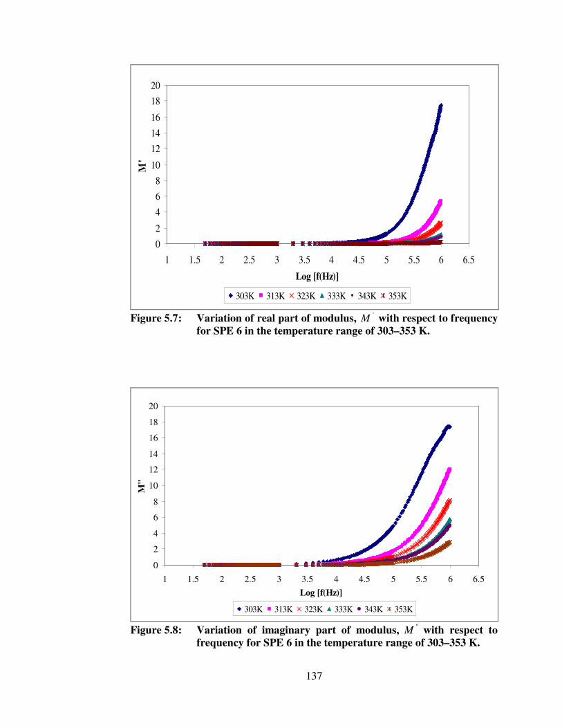
137
02
468
10
121416
1820
1 1.5 2 2.5 3 3.5 4 4.5 5 5.5 6 6.5
Log [f(Hz)]
M'
303K 313K 323K 333K 343K 353K
Figure 5.7: Variation of real part of modulus, 'M with respect to frequency for SPE 6 in the temperature range of 303–353 K.
0
2
4
6
8
10
12
14
16
18
20
1 1.5 2 2.5 3 3.5 4 4.5 5 5.5 6 6.5Log [f(Hz)]
M''
303K 313K 323K 333K 343K 353K
Figure 5.8: Variation of imaginary part of modulus, ''M with respect to frequency for SPE 6 in the temperature range of 303–353 K.

138
5.7 HATR–FTIR studies
The HATR–FTIR spectra of SPE 3, SPE 6 and SPE 8 are illustrated in
Figures 5.9 (a)–(c). In contrast, the comparison of HATR–FTIR spectra for
PMMA–PVC, pure LiTFSI, SPE 3, SPE 6 and SPE 8 are shown in Figure 5.10.
Table 5.1 shows the designations of the characteristic peaks of PMMA, PVC and
LiTFSI for SPE 6 system. The HATR–FTIR spectrum of SPE 6 is further
discussed as it achieves the maximum ionic conductivity in the study. There are
five new peaks appearing by comparing SPE 6 with PMMA–PVC. These new
peaks are assigned as combination of C–S and S–N stretching mode of LiTFSI, C–
SO2–N bonding mode of LiTFSI, SO2 asymmetric stretching mode of LiTFSI and
S–CH3 bonding mode of LiTFSI at 791 cm-1, 1327 cm-1, 1349 cm-1, 2845 cm-1 and
2997 cm-1, respectively. It indicates that there is an establishment for formation of
polymer salt system.
Figure 5.9 (a): HATR–FTIR spectrum of SPE 3.

139
Figure 5.9 (b): HATR–FTIR spectrum of SPE 6.
Figure 5.9 (c): HATR–FTIR spectrum of SPE 8.

140
Figure 5.10: Combination of HATR–FTIR spectra for (a) PMMA–PVC, (b)
pure LiTFSI, (c) SPE 3, (d) SPE 6 and (e) SPE 8.
Description vibration modes Wavenumber (cm-1)
References
Cis C–H wagging mode of PVC 708 Rajendran et al., 2008
Combination of CH2 rocking of PMMA and S–N stretching of LiTFSI
746 Rajendran et al., 2008; Ahmad et al.,
2008 Combination of C–S and S–N stretching mode of LiTFSI
791 Ahmad et al., 2008
C–Cl stretching of PVC 847 Li et al., 2006a Trans C–H wagging mode of PVC 910 Achari et al., 2007 Combination of C–O symmetric stretching mode in C–O–C linkage of PMMA and trans C–H wagging mode of PVC
963 Achari et al., 2007
CH2 wagging mode of PMMA 981 Rajendran et al., 2002
Combination of C–H rocking mode of PVC and S–N–S asymmetric bonding mode of LiTFSI
1056 Achari et al., 2007; Ahmad et al., 2008
Combination of C–O asymmetric stretching mode in C–O–C linkage of PMMA and C–SO2–N bonding mode of LiTFSI
1133 Jiang et al., 2006; Ramesh and Lu,
2008
Combination of CH2 twisting mode of 1186 Rajendran et al.,

141
PMMA and CF3 symmetric stretching mode of LiTFSI
2004; Ahmad et al., 2008
CH3 symmetric bending mode of PMMA 1232 Jiang et al., 2006 C–O–C symmetric stretching mode of PMMA
1284 Jiang et al., 2006
C–SO2–N bonding mode of LiTFSI 1327 Ramesh and Lu, 2008
SO2 asymmetric stretching mode of LiTFSI
1349 Ahmad et al., 2008
Combination of CH3 asymmetric bending mode of PMMA and C–H stretching mode of CH2 group of PVC
1444 Rajendran et al., 2004; Rajendran et
al., 2008 C=C stretching mode of PVC 1661 Achari et al., 2007 C=O stretching mode of PMMA 1711 Li et al., 2006a S–CH3 bonding mode of LiTFSI 2845, 2997 Ramesh and Lu,
2008 CH3 asymmetric stretching mode of PMMA and PVC
2926 Achari et al., 2007; Rajendran et al.,
2008 Table 5.1: Assignments of vibrational modes of PMMA, PVC and LiTFSI
for SPE 6 polymer matrix system.
As shown in Figure 4.9 (c), a weak peak which designated as C–H rocking
mode of PVC is observed in PMMA–PVC spectrum. However, this peak is
disappeared in comparison to SPE 6 spectrum. It is suggestive of overlapping with
S–N–S asymmetric bonding mode of LiTFSI, indicating the interaction between
polymer blends and LiTFSI. In order to prove the complexation between polymer
blends and LiTFSI, the changes in intensity and changes in shape of the
characteristic peak are probed further.
Besides, there is an obvious change in shape for the S–CH3 bonding mode
of LiTFSI in the region of 2979–2876 cm-1. In the pure LiTFSI spectrum, it
appears as two sharp peaks; however, it appears as a single peak with two small
shoulders after incorporation with PMMA–PVC polymer blend matrix. It is due to

142
overlapping of C–H stretching mode of PMMA, C–H stretching mode of PVC and
S–CH3 bonding mode of LiTFSI. This reveals that there is a binding of PMMA,
PVC and LiTFSI. Apart from that, a distinctive change of characteristic absorption
in the region of 1186–1133 cm-1, that is from a single peak with a small shoulder
to double peaks is illustrated in Figure 5.11. In this region, 1133 cm-1 is assigned
as combination of C–O asymmetric stretching mode in C–O–C linkage of PMMA
and C–SO2–N bonding mode of LiTFSI, whereas 1186 cm-1 is assigned as
combination of CH2 twisting mode of PMMA and CF3 symmetric stretching mode
of LiTFSI. The change in shape for latter peak may attributed to the occurrence of
an interaction of CH3 in PMMA and CF3 in LiTFSI via coordination bond
involving hydrogen bond of hydrogen atom of PMMA with fluorine atom of
LiTFSI leading to a complexation between PMMA and LiTFSI. This discloses the
interaction between PMMA and LiTFSI.
Figure 5.11: The comparison of change in shape of overlapping asymmetric
O–CH3 stretching mode of PMMA and symmetric stretching mode of CF3 of LiTFSI in (a) PMMA–PVC and (b) SPE 6.

143
Upon addition of 30 wt% of LiTFSI, some characteristic peaks exhibit
changes in shift. The characteristic peaks of cis C–H wagging mode of PVC, C–Cl
stretching mode of PVC, CH2 wagging mode of PMMA and C=C stretching mode
of PVC are shifted from 698 cm-1, 842 cm-1, 983 cm-1 and 1684 cm-1 to 708 cm-1,
847 cm-1, 981 cm-1 and 1661, respectively. It divulges that there is an interaction
between PMMA, PVC and LiTFSI. The CH2 rocking mode of PMMA at 751 cm-1
is shifted to 746 cm-1 due to the overlapping with S–N stretching of LiTFSI.
However, the combination of C–O symmetric stretching mode in C–O–C linkage
of PMMA and trans C–H wagging mode of PVC remains unchanged at 963 cm-1.
Apart from that, the intensity of characteristic absorption peaks has also been
changed. As exemplified in Figure 5.12, there is an observable change in intensity
in C=O stretching mode of PMMA at 1711 cm-1. Intensity of this sharp peak
increases by 1.35 % in transmittance mode, which is from 1.90 % to 3.25 %;
meanwhile it also undergoes shifting in wavenumber that is shifted from 1725 cm-1.
It might due to an interaction of C=O of ester in PMMA with LiTFSI via
coordination bond.
Similarly, the intensity of combination of CH3 asymmetric bending mode
of PMMA and C–H stretching mode of CH2 group of PVC at 1444 cm-1 is also
enhanced by 0.54 % after addition of LiTFSI. It changes from 0.6 % to 1.14 %,
whereas it changes from 1436 cm-1 to 1444 cm-1 in terms of shift in peak. Again,
this reveals the interaction between polymer blends and LiTFSI. On the contrary,
the intensity of CH3 symmetric bending mode of PMMA is reduced by 0.80 %,
which is from 1.20 % in PMMA–PVC spectrum and this peak is shifted from 1244

144
cm-1 to 1232 cm-1. It signifies the coordination bonding between PVC and LiTFSI.
Based on these results, it denotes the presence of complexation between PMMA,
PVC and LiTFSI.
Figure 5.12: The comparison of change in intensity of C=O stretching mode
of PMMA in (a) PMMA–PVC and (b) SPE 6.
All the vibrational modes of SPE 3, SPE 6 and SPE 8 have been shown in
Figure 5.9 (a)–(c). However, cis C–H wagging mode of PVC is absent in SPE 8. In
order to further investigate the ion aggregation, the bands in the wavenumber
region of 1400–1100 cm-1 were explored (Ahmad et al., 2008). There are some
obvious changes in shift at 1327 cm-1 and 1349 cm-1. The first peak is assigned as
C–SO2–N bonding mode of LiTFSI, whereas SO2 asymmetric stretching mode of
LiTFSI is for latter peak. Both Figures 5.9 (a) and (b) show a peak at 1349 cm-1

145
with a shoulder at 1327 cm-1. However, upon further addition of LiTFSI, the peak
is shifted to 1352 cm-1, whereas the shoulder peak is shifted to 1330 cm-1, as
shown in Figure 5.9 (c). These upward shifts reveal the ion aggregation of LiTFSI,
which in turn to impede the ionic transportation within the polymer matrix. In
other words, reduction in ion pairing is occurred at lower frequency in SPE 3 and
SPE 6.
5.8 XRD Studies
XRD analysis has been performed and their respective diffraction patterns
of PMMA–PVC, pure LiTFSI, SPE 3, SPE 6 and SPE 8 are shown in Figure 5.13
(a)–(e). Sharp diffraction peaks appear at 2�=13.6°, 15.9°, 18.6°, 18.9° and 21.4°
reveals the crystalline behavior of pure LiTFSI. All these peaks pertaining to
LiTFSI are absent, indicating the absence of uncomplexed excessive LiTFSI and
no separate phase in the SPE 3 and SPE 6 polymer systems (Saikia and Kumar,
2004; Rajendran et al., 2008). Hence, it divulges that there is a complete
dissolution of LiTFSI in the polymer complexes and form complexation between
PMMA–PVC with LiTFSI as well as inhibits crystallization (Sivakumar et al.,
2007). However, there is a sharp peak at 2�=13.8° for SPE 8 and this indicates the
presence of excessive LiTFSI salt precipitation. These bulky ion associations
obstruct the Li+ cations transportation and leading to decreases in ionic
conductivity as demonstrated in Figure 5.14. As shown in Figure 5.12(a), two
broad peaks are observed at 2�= 15.8° and 22.3° for PMMA–PVC polymer blends,

146
revealing the amorphous characteristic of PMMA–PVC polymer blends. However,
these peaks are shifted to 2� value of 17.1° and 22°, 16.9° and 22.6° and 16° and
22.3° for SPE 3, SPE 6 and SPE 8, respectively upon addition of LiTFSI. This
shift indicates the complexation between polymer blends and lithium salt
(Sivakumar et al., 2006). Another evidence to prove the complexation of PMMA–
PVC with LiTFSI is observed. Upon inclusion of LiTFSI, the decrease in the peak
width of characteristic peaks is the apparent proof.
A discernible change in peak width and relative intensity of characteristic
peaks for SPE 6 is illustrated in Figure 5.13. These apparent peaks become broader
and intensity is reduced upon addition of 30 wt% of LiTFSI. Based on these
observations, it reveals more amorphous region of SPE 6 than SPE 3 and SPE 8
and forms disorder arrangement in the polymer matrix. This significant disorder
induces a more flexible polymer backbone and thus enhancing ionic transportation.
Similarly, the peaks of SPE 3 are slightly sharper than SPE 8. This suggesting SPE
8 exhibits higher degree of amorphous as sharper of apparent peaks indicating
higher degree of crystallinity (Saikia and Kumar, 2004). This result is consistent
with the coherence length measurement. The coherence length of these polymer
electrolytes was determined for the peak at 2�≈ 16°.
From Figure 5.14, the coherence length of SPE 8 is higher than SPE 3. In
general, coherent length defines as crystallite size. As the diffraction peak width is
longer, the crystallite size is shorter, and hence contributing to lower crystallinity
(Aravindan et al., 2009). Therefore, it is another evidence to prove the higher

147
amorphousity of SPE 8 than SPE 3. In addition, this result in good agreement with
ionic conductivity at ambient temperature as illustrated in Figure 5.14. From this
figure, ionic conductivity of SPE 8 is higher than SPE 3. Higher degree of
amorphous of polymer matrix attributes to more disorder arrangement of
polymeric chain and thus increases flexibility of polymer matrix. The flexible
backbone increases the mobility and concentration of charge carrier. As a result,
more voids are formed into the polymer system, promoting the ionic transportation
and thus leading ultimately to highest ionic conductivity at room temperature. As
discussed earlier, SPE 6 exhibits highest degree of amorphous. It is further proven
in coherence length measurement by showing the shortest value. It might be due to
the concentration and mobility had reached the optimum level, inferring the
highest ionic conductivity of SPE 6 as illustrated in Figure 5.14.
0 10 20 30 40 50 60 70 802�(°)
Inte
nsity
(a.u
)
Figure 5.13: XRD patterns of (a) PMMA–PVC, (b) pure LiTFSI, (c) SPE 3,
(d) SPE 6 and (e) SPE 8.
(d)
(a)
(b)
(c)
(e)

148
0
0.2
0.4
0.6
0.8
1
1.2
0 15 30 40
Percentage of LiTFSI (% wt)
Coh
eren
ce le
ngth
(Å)
-12
-10
-8
-6
-4
-2
0
Log
� [l
og (S
cm-1
)]
Coherence length (Å) Log �
Figure 5.14: Variation of coherence length logarithm of ionic conductivity at ambient temperature with respect to different mole fraction of LiTFSI into PMMA–PVC polymer blends–based polymer electrolytes at 2�≈ 16°C.
5.9 SEM Studies
Figures 5.15 (a)–(c) depict SEM images of SPE 3, SPE 6 and SPE 8
polymer electrolytes, respectively. SPE 3 membranes illustrate coarse texture,
indicating that the higher crystallinity. In contrast, SPE 6 and SPE 8 polymer
systems have higher amorphous region by illustrating a smooth surface onto these
systems (Baskaran et al., 2007). Figure 5.15 (a) has shown some craters with
average pore size around 1 �m. The effect of rapid volatilization of THF solvent
during preparation is a contributor of this phenomenon (Rajendran et al., 2000a).
The decrease in these craters might be due to the interaction between LiTFSI and
polymer blends. An evident change in shape of pores is observed in this study.

149
Upon dispersion of LiTFSI, it has been changed from rectangular to spherical
shape by comparing Figure 4.19 (c) with Figures 5.15 (a)–(c). This is mainly due
to the disruption of LiTFSI onto polymer blends via coordination bonding between
Li+ cations with electron–rich group, such as oxygen from PMMA where the
coordinating sites are C–O–C and C=O.
According to Figure 5.15 (a), the pores with size of 9–20 �m are observed.
These pores are much larger than SPE 6 and SPE 8 and assigned to the coagulation
of PMMA–PVC. Thus, the complexation of LiTFSI with PMMA–PVC polymer
blends is lesser. Therefore, the Li+ cations migration is unfavorable and induces to
lower ionic conductivity. In addition, these aggregates are surrounded by fine
streak with average size of 1 �m and suggesting the PMMA–PVC polymer blend
is bounded by LiTFSI salt and thus LiTFSI salt starts to interact with PMMA–
PVC. Eventually, it forms complexation with PMMA–PVC polymer blends.
Similarly, some fine spherical cavities with average size of 1 �m are observed in
Figure 5.15 (c), which mainly due to LiTFSI salt precipitation (Baskaran et al.,
2007). At high LiTFSI loadings, the salts tend to exist in ion pairs rather than form
complexation with PMMA–PVC polymer blends. These aggregated ions lead to
more crystalline phase in this polymer electrolyte. Eventually, these crystalline
regions hinder the ionic mobility in this polymer membrane. This observation is in
good agreement with HATR–FTIR and XRD analyses.
On the contrary, Figure 5.15 (b) demonstrates a well distribution of pores
in oval shape within similar dimension, with average size of 6 �m in the polymer

150
matrix. This infers the well dissolution of LiTFSI and high homogeneity of
polymer electrolyte with lesser agglomerates (Fonseca et al., 2009). This even
distribution attributed to excellent complexation between LiTFSI and PMMA–
PVC, which in turn to promote the migration of ions and eventually leads to higher
ionic conductivity. Generally, the main role of pores is to act as a passage for Li+
cations during charge–discharge cycle (Uma et al., 2005). Higher porosity of SPE
6 is also exemplified in this figure and revealing the higher ions shipping.
Figure 5.15 (a): SEM image of SPE 3.

151
Figure 5.15 (b): SEM image of SPE 6.
Figure 5.15 (c): SEM image of SPE 8.

152
5.10 DSC Studies
Only one gT appears for all the samples indicating the homogenous
samples as shown in Figure 5.16 (Ahmad et al., 2006b). gT is shifted towards
higher temperature upon incorporation of LiTFSI as shown in Table 5.2. This
might be due to the formation of transient self cross–linking as a result of
coordination between Li+ cations with the electron–withdrawing groups, such as –
O– and C=O functional groups (Li et al., 2006a). This binding energy increases
the barrier of the polymer matrix and reduces the degree of mobility of polymer
segments. Therefore, the polymer backbone becomes less flexible (Ramesh and
Arof, 2001b).
As expected, gT is decreased with increasing the LiTFSI concentration. gT
decreases from around 125 °C to 118 °C by adding more 15 wt % of LiTFSI and
this result is clearly depicted in Table 5.2. Plasticizing effect of LiTFSI is the main
contributor. As increases LiTFSI loadings, salts tend to exist in ion pairs or ion
clusters between polymer matrix and thus lead to weaken the dipole–dipole
interactions. As a result, the transient cross–linkage between polymer matrix is
absent and resulting a decreases in solvation of Li+ cations with oxygen of ester
functional group from PMMA. Eventually, a softer polymer backbone is formed
and resulting in enhancement of segmental motion and flexibility of polymer
matrix (Baskaran et al., 2007). Thus, more voids are formed as the segmental
mobility is increased. Therefore, Li+ cations are easier to migrate in this polymer

153
matrix when the electric field is applied (Ramesh and Arof, 2001b). However, gT
is increased with addition of 40 wt% of LiTFSI. This is suggestive of increases in
formation of inter–self crosslinking bonds between LiTFSI and polymer blends
with excessive addition of LiTFSI, leading to higher barrier for rotation in the
polymer chain and hence, flexibility of polymer chain becomes lesser by lowering
degree of segmental movement in the polymer chain (Yang et al., 2008a).
Beyond gT , heat flow of polymer matrix becomes stable up to above 160
°C, a distinct endothermic peak is observed and denotes as broad melting point of
electrolyte, mT . The broadening of this endothermic peak is assigned to
overlapping of melting point of both PMMA and PVC. Thus, it is followed by a
stable range of heat flow again over the temperature regime and then a visible
sharp peak endothermic peak is obtained at above 300 °C. After that, a small
endothermic peak is also observed as shown in Figure 5.16. These peaks are
corresponding to decomposition temperature of polymer electrolyte, dT .
Obviously, SPE 6 exhibits highest melting temperature. This implies that the
thermal properties of polymer electrolytes are enhanced with adulteration of 30
wt% of LiTFSI.
Moreover, the initial dT is associated with dehydrochlorination of PVC
which initiated by Cl free radical (Ahmad et al., 2007), whereas the second
relatively small dT is attributed to the degradation of unsaturated group from
PMMA, such as C–O bonds and degradation of PVC (Ahmad et al., 2006b).
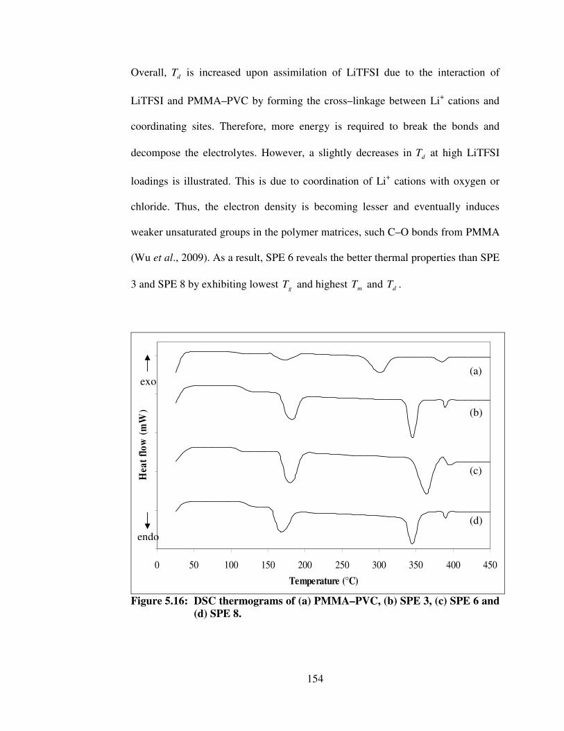
154
Overall, dT is increased upon assimilation of LiTFSI due to the interaction of
LiTFSI and PMMA–PVC by forming the cross–linkage between Li+ cations and
coordinating sites. Therefore, more energy is required to break the bonds and
decompose the electrolytes. However, a slightly decreases in dT at high LiTFSI
loadings is illustrated. This is due to coordination of Li+ cations with oxygen or
chloride. Thus, the electron density is becoming lesser and eventually induces
weaker unsaturated groups in the polymer matrices, such C–O bonds from PMMA
(Wu et al., 2009). As a result, SPE 6 reveals the better thermal properties than SPE
3 and SPE 8 by exhibiting lowest gT and highest mT and dT .
0 50 100 150 200 250 300 350 400 450
Temperature (°C)
Hea
t flo
w (m
W)
Figure 5.16: DSC thermograms of (a) PMMA–PVC, (b) SPE 3, (c) SPE 6 and
(d) SPE 8.
(a)
(b)
(c)
(d) endo
exo

155
DSC measurements Designations
gT (°C) mT (°C) dT (°C)
PMMA–PVC 105.40 175.54 305.38, 385.40 SPE 3 125.21 163.83 345.50, 389.23 SPE 6 118.16 184.50 366.20, 390.27 SPE 8 127.11 165.67 343.83,389.46
Table 5.2: DSC measurements of PMMA–PVC–LiTFSI based polymer electrolytes.
5.11 TGA Studies
According to Figure 5.17, three apparent segments are observed for all the
samples. Initially, 2–4 % of weight loss is attained at 172 °C, 121 °C, 139 °C and
130 °C for PMMA–PVC, SPE 3, SPE 6 and SPE 8, respectively. This first small
weight loss discloses the evaporation process of residue THF solvent and
elimination of impurities which mainly due to fluorine compound from LiTFSI.
Besides, dehydration of moisture is also a contributor for this phenomenon as the
tendency of polymer to absorb water from surrounding is quite high.
Above this initial weight loss, it remains stable up to above 252 °C for
PMMA–PVC, 269 °C for SPE 3, 288 °C for SPE 6 and 279 °C for SPE 8. At this
temperature, it starts to degrade and forms second significant weight loss. The
weight losses of 59 % and 35 % at 342 °C and 349 °C are obtained for PMMA–
PVC and SPE 3, respectively. In contrast, 26 % mass loss is appeared at 348 °C
for SPE 6. For SPE 8, weight loss at 339 °C corresponds to 30.3 % is achieved.
The second significant weight loss is mainly due to the unzipping process which

156
contributed a reduction in molecular weight of polymer chain at high temperature.
This unzipping reaction causes many degradation reactions such as random chain
scission reaction, depolymerization, intra–molecular transfer reaction whereby
dimer, trimers and oligomers are produced and inter–molecular transfer reaction as
well as polymer fragments. As a result, the monomer and oligomers which chemi–
adsorbed onto the polymer matrix is volatilized in this temperature regime (Ahmad
et al., 2007). Besides, another attributor is the dehydrochlorination reaction from
PVC, as proven in DSC thermogram.
A gradual weight loss is followed up thereafter. For PMMA–PVC and SPE
3, around 31 % and 24 % of mass losses, with residual mass of 28 % and 41 % are
shown at 385 °C and 389 °C, respectively. Smaller weight losses are obtained for
SPE 6 and SPE 8. SPE 6 has around 11 % weight loss at 390 °C, with residual
mass of 60.35 %, whereas around 21 % of mass loss, with residual weight of 45 %
at 389 °C is observed clearly for SPE 8. Above 400 °C, the baseline remains stable
and hence indicates the end of the thermal decomposition of the polymer
electrolytes (Fonseca et al., 2009). As a conclusion, SPE 6 is a promising
candidate because its thermal stability is up to 288 °C and greatly preferred in
lithium polymer batteries as its operating temperature is normally in the range of
40–70 °C (Stephan et al., 2002).

157
20
30
40
50
60
70
80
90
100
110
0 50 100 150 200 250 300 350 400 450Temperature (°C)
Wei
ght (
%)
PMMA-PVC SPE 3 SPE 6 SPE 8
Figure 5.17: Thermogravimetric analysis of PMMA–PVC, SPE 3, SPE 6 and SPE 8.
5.12 Amplitude Sweep
Figure 5.18 shows the logarithm scale of amplitude sweep of this polymer
electrolyte system. According to the figure, the yield point is absent within the
strain regime and there is no behavioral transition in this polymer complex
(Fonseca et al., 2009). Elongation of samples is produced when stress is applied.
Different evident trends are observed with addition of LiTFSI. At high strain,
PMMA–PVC polymer blends shows a slow decrement. Nevertheless, the LiTFSI–
based polymer electrolytes decrease rapidly at high strain. It divulges that the
elastic properties decrease in favor of viscous properties at higher elongation of
28.32%
40.88%
60.35%
44.91%

158
sample when the stress is applied. This is attributed to the broken down of the
structures of the sample once the stress is applied on the samples. All the samples
show that 'G values are greater than ''G within the elongation range, implying the
predominant solid nature of all the samples. Upon inclusion of LiTFSI, at 0.001%
strain, both 'G and ''G values increases by more than an order of magnitude,
indicating the solid–like medium of samples. Hydrogen bonding might be an
attributor as it forms the complexation between LiTFSI and polymer blends. It can
be seen that the hydrogen atom of polymer blends is readily reacted with oxygen
atom of LiTFSI and contributes to the complexation. These hydrogen bonds
initiate the entanglements within the polymer matrix and eventually lead to higher
solid components in the samples.
The values of 'G and ''G decrease with increasing the LiTFSI mass
fraction. It is primarily correlated to the plasticizing effect of LiTFSI. This helps in
softening the polymer backbone and thus further reduces the crystalline region of
the sample. Amorphous is pre–dominant and therefore weakens the interaction
between the molecular bonding of polymer matrix. Consequently, the elastic
properties of polymer electrolytes are decreased at higher concentration of LiTFSI.
As shown in Figure 5.18, the interval between 'G and ''G of SPE 6 decreases
sharply compared to SPE 3. This indicates that the viscous behavior is increased,
meanwhile the solid properties is destroyed. However, for SPE 8, both values of
'G and ''G are increased somewhat due to the precipitation of excessive salt in the
polymer system. This agglomeration of salt increases the solid nature of polymer
blends systems. Among SPE 3, SPE 6 and SPE 8, SPE 6 illustrates the widest LVE

159
range. It proposes that the structural stability of SPE 6 is the highest and it is
difficult to be deformed.
10
100
1000
10000
100000
0.001 0.01 0.1 1 10 100 1000 Strain (%)
G' a
nd G
'' (P
as)
PMMA-PVC(G') PMMA-PVC(G'') SPE 3(G') SPE 3(G'')SPE 6(G') SPE 6(G'') SPE 8(G') SPE 8(G'')
Figure 5.18: Oscillatory shear sweeps for PMMA–PVC, SPE 3, SPE 6 and
SPE 8.
C
H
C C C
H
H H H
C l C l
n
H C
O
C O
C C H 2C H 2C
C H 3
C
O
O H
C H 3
H O S N
C F 3
O
S C F3
O
OLi
n
Figure 5.19: Hydrogen bonding between LiTFSI and polymer blends.

160
5.13 Oscillatory Stress Sweep
Figure 5.20 shows oscillatory shear sweeps of PMMA–PVC, SPE 3, SPE 6
and SPE 8 on logarithm scale. For all the samples, the values of 'G are greater
than ''G , indicating that the solid properties domain in the polymer matrices. The
crossover of 'G and ''G is absent within the range of shear stress. This important
feature indicates that there is no behavioral transition in the polymer electrolytes
(Fonseca et al., 2009). 'G increases with dispersion of LiTFSI due to the
occurrence of complexation through the hydrogen bonding. The solid behavior of
the samples is further confirmed in this oscillatory shear sweep. As explained in
section 5.12, 'G and ''G values decrease with incorporation of 30 wt% of LiTFSI,
but, they are enhanced as 10 wt% of LiTFSI were further added in the polymer
electrolyte system. This result is in good agreement with the amplitude sweep
study. The first phenomenon is mainly due to the plasticizing effect, whereas the
agglomeration of salt is an attributor for latter trend. An insignificant reduction in
'G and ''G is observed at initial part. It is suggestive of initial interruption of the
polymer structures when some forces are applied on the samples. On the other
hand, the sharp decrease at the end region is attributed to the destruction of the
chemical bonding between the polymeric systems.
For the initial shear stress, PMMA–PVC illustrates the lowest value. In
other words, the deformation of PMMA–PVC compound can be arisen easily by
applying a small amount of small forces and reveals the lowest mechanical

161
stability. As explained above, the solid behavior of LiTFSI–based polymer
electrolytes is increased. Since the solid behavior is increased, therefore the
mechanical strength is also improved with impregnation of LiTFSI. It can further
been proven in this study by increasing the amount of shear stress. It is expected
that more shear stress is required to deform the LiTFSI–based polymer electrolytes.
SPE 3 shows higher shear stress in comparing with PMMA–PVC due to the
formation of coordination bonding between LiTFSI and polymer blends. However,
SPE 6 depicts lower shear stress and thereby asserting the ease distortion of this
sample. It might be associated with plasticizing effect of LiTFSI. In general, the
plasticizing effect assists to destroy the dipole–dipole interactions, which in turn to
the enhancement of segmental motion and flexibility of polymer matrix. Therefore,
less energy is needed to break the bonds in the polymer complex. In contrast, the
quantity of shear stress applied on SPE 8 is higher due to the salt agglomeration
and this effect compensates the plasticizing effect. The salts have a tendency to
form aggregation when the salts loadings are in excess. More stress is required to
break the bonds among the aggregates, and thus the mechanical stability is
enhanced.

162
10
100
1000
10000
100000
0.001 0.01 0.1 1 10 100 1000 10000Shear stress (Pa)
G' a
nd G
'' (P
as)
PMMA-PVC(G') PMMA-PVC(G'') SPE 3(G') SPE 3(G'')SPE 6(G') SPE 6(G'') SPE 8(G') SPE 8(G'')
Figure 5.20: Amplitude sweeps of PMMA–PVC, SPE 3, SPE 6 and SPE 8.
5.14 Oscillatory Frequency Sweep
The frequency sweeps of PMMA–PVC, SPE 3, SPE 6 and SPE 8 are
shown in Figure 5.21. The disappearance of ''G confirms once again the solid–
like of all the samples. Again, same observations are obtained for second system in
comparison to first polymer electrolyte system. Two visible regions are observed
within the frequency range. 'G exhibits frequency–dependent at low frequency,
meanwhile an almost constant region is detected at high frequency. At high
frequency, the value of elastic properties of polymer electrolytes is higher for
short–term of deformation and it is attributed to short relaxation time. The polymer
chain is unable to slip past one another and thus increases the ability of the
unmoved polymer chain to store the imposed energy, leading to more elastic

163
properties of the sample (Ebagninin et al., 2009). However, the structural strength
has been changed when the deformation takes place for a prolonged time. The
relaxation time becomes longer and the slippage of the entanglements of the
polymeric chain is available. The ability of polymer chain to store the elastic
energy is reduced. As a result, the solid behavior becomes lesser at low frequency.
At the highest frequency (0.1 rads-1), 'G values of all the samples are
almost the same. All the samples exhibit the same elastic energy at this frequency
and indicate that the addition of LiTFSI does not bring up any effect on the
structural stability at high frequency. However, the 'G values are varied as the
frequency is decreased. This describes the different long–term structural stability
of each sample. PMMA–PVC compound manifests higher structural stability by
showing the least decrease in 'G . The 'G values are relatively decreased upon
inclusion of LiTFSI. In comparing of all LiTFSI–based polymer electrolytes, the
decrease in 'G values is in this order: SPE 8 > SPE 3 > SPE 6. The larger amount
of 'G of SPE 8 is due to the salt precipitation. The coordination bonds among the
salt aggregates induce to a difficulty on the slippage process. Therefore, the elastic
properties are gradually decreased. Plasticizing effect is the contributor for the
lowering in 'G value. As explained in previous study, the plasticizing effect of
LiTFSI weakens the dipole–dipole interaction. After a long–term of deformation
timeline, the LiTFSI is further weakens those physical and chemical interactions
within the polymer matrix, such as the cross–linking between PMMA and PVC,
promoting the mobility of polymer segments. Thus, the entanglements among the
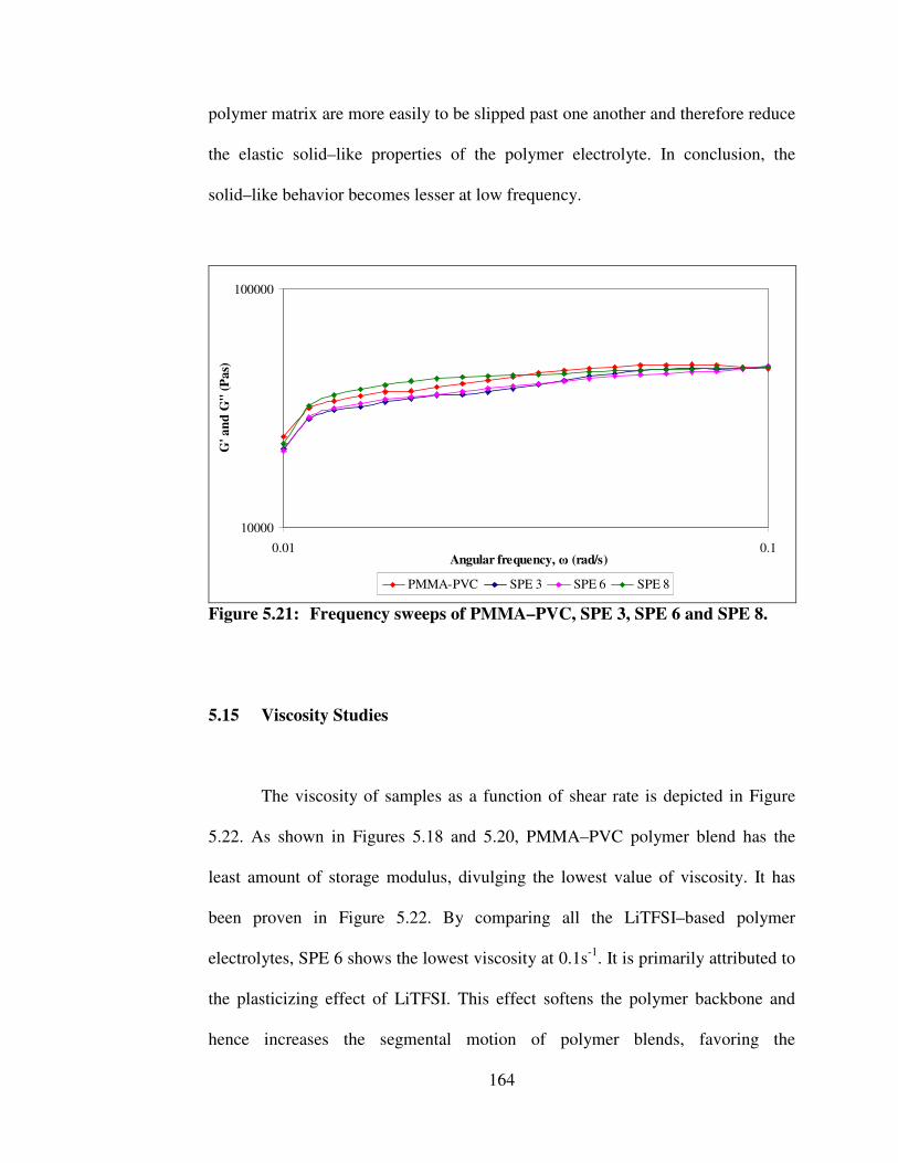
164
polymer matrix are more easily to be slipped past one another and therefore reduce
the elastic solid–like properties of the polymer electrolyte. In conclusion, the
solid–like behavior becomes lesser at low frequency.
10000
100000
0.01 0.1Angular frequency, � (rad/s)
G' a
nd G
'' (P
as)
PMMA-PVC SPE 3 SPE 6 SPE 8
Figure 5.21: Frequency sweeps of PMMA–PVC, SPE 3, SPE 6 and SPE 8.
5.15 Viscosity Studies
The viscosity of samples as a function of shear rate is depicted in Figure
5.22. As shown in Figures 5.18 and 5.20, PMMA–PVC polymer blend has the
least amount of storage modulus, divulging the lowest value of viscosity. It has
been proven in Figure 5.22. By comparing all the LiTFSI–based polymer
electrolytes, SPE 6 shows the lowest viscosity at 0.1s-1. It is primarily attributed to
the plasticizing effect of LiTFSI. This effect softens the polymer backbone and
hence increases the segmental motion of polymer blends, favoring the

165
disentanglements within the polymer matrix. As a result, it reduces the viscosity
and hence increases the amorphous proportion which accompanied with higher
ionic transportation within the polymer electrolytes. Theoretically, the viscosity of
SPE 8 would be the lowest as it is embedded with higher LiTFSI compositions.
However, it is higher than SPE 6 due to the salt precipitation in the polymer
system. Weak physical bonds are formed among the salt aggregates and leads to a
reduction of the movement of polymer chain. Hence, the viscosity is increased
with formation of this network structure. SPE 3 has highest viscosity because of
insufficient of the plasticizing effect.
All samples exhibit downward shift in viscosity as increases in shear rate,
implying the shear thinning behavior (Ahmad et al., 2005). The occurrence of
non–newtonian characteristic is due to the rupture of structure and bonding among
the polymer matrix with increasing the shear rate. It commonly denotes as
disruption of inherent self–crosslinking between PMMA and PVC. For LiTFSI–
based polymer electrolytes, the hydrogen bonding between LiTFSI and polymer
blends has also been destroyed. The interactions between those excessive salt
aggregates are being interrupted for SPE 8 as well. The values of viscosity are
almost the same at the highest shear rate of 100s-1. This suggests that the addition
of LiTFSI does not possess any contribution to the viscosity when high shear is
applied.

166
0.1
1
10
100
1000
10000
0.1 1 10 100Shear rate (1/s)
Visc
osity
, � (P
as)
PMMA-PVC SPE 3 SPE 6 SPE 8
Figure 5.22: Typical viscosity curve of PMMA–PVC, SPE 3, SPE 6 and SPE 8.
5.16 Summary
PMMA–PVC polymer blends electrolytes are prepared by solution casting
technique. Based on all the analyses, 70 wt % PMMA–PVC polymer blends and
30 wt % LiTFSI as dopant salt is found to be better choice as a polymer electrolyte
in lithium batteries. In this present work, the highest ambient temperature–ionic
conductivity of (1.11±0.09)×10-6 Scm-1 was achieved upon addition of 30 wt%
LiTFSI salt. The temperature dependence study obeys Arrhenius rules and it obeys
Jonscher’ s universal law for frequency dependence study. Both of these laws
suggest the occurrence of hopping mechanism in the polymer matrix. In dielectric
relaxation study, the polarization effect is the main contributor to increase these 'ε
and ''ε values at low frequency region. Only bulk effect can be observed in the

167
variation of 'M and ''M at high frequency regime. The ac–impedance and
dielectric study reveals the occurrence of non–Debye characteristic of polymer
electrolytes. Based on HATR–FTIR analysis, there is a complexation between
PMMA, PVC and LiTFSI with the presence of new peaks, change in shift, change
in intensity and change in shape.
XRD result had shown the shortest coherence length and reveals the high
degree of amorphous in this polymer electrolyte. High porosity is also divulging
the higher degree of ionic transportation in the polymer matrix as illustrated in
SEM. From DSC and TGA measurements, an excellent thermal property of the
polymer matrix is observed. From DSC analysis, gT is lowered which produces a
more flexible polymer backbone, whereas highest mT and dT are achieved.
Thermal stability is well enhanced upon addition of 30 wt % of LiTFSI and this
result is proven in TGA analysis.
Elastic properties are much higher than viscous properties within the range
as shown in the amplitude sweep and oscillatory shear sweep studies. The
disappearance of crossover of 'G and ''G indicates the absence of behavior
transition. The viscous behavior is absent in the frequency sweep and indicates the
solid–like characteristic within the frequency regime. At low frequency, solid
properties of polymer electrolytes reduced when the deformation takes place for a
prolonged time, denoting the lower structural strength of polymer electrolytes. The
viscosities of all the samples are decreased with increasing the shear rate.

168
CHAPTER 6
RESULTS AND DISCUSSION OF THIRD POLYMER BLEND
ELECTROLYTES SYSTEM
6.1 AC–Impedance Studies
Figures 6.1 and 6.2 depict the complex impedance diagrams for IL 2, IL 5
and IL 6 at ambient temperature. In general, the electrolyte–electrode interface is
regarded as capacitance and a vertical spike is observed while the capacitance is in
ideal mode (Stephan et al., 2000b). However, a spike is inclined at an angle of 90°
to the real axis as shown in Figures 6.1 and 6.2. This implies the non–idealism of
capacitance properties and leads to ionic polarization at the blocking electrodes.
As a consequence, a constant phase element (CPE) is present in the electrolyte–
electrode interface and it is known as non–Debye nature (Venkateswarlu et al.,
2000). The amounts of inclined slope and angle indicate the roughness of the
electrolyte surface and distribution of relaxation time (Stephan et al., 2000b;
Venkateswarlu et al., 2000). For this relaxation distribution, these charge carriers
are accumulated at the electrode and electrolyte interface before the electric field
changes the direction.
Obviously, two regions: a slanted spike at low frequency and a semicircle
at high frequency are observed in Figure 1. This divulges the parallel combination

169
of bulk resistance ( bR ) and bulk capacitance ( pC ) effects of the polymeric
electrolyte in the conduction process. Resistance is related to the ionic migration
among the polymer matrix and represented by resistor at lower frequency, whereas
the polarization of immobile polymer chain in the alternating field is represented
by capacitor at higher frequency (Ramesh and Arof, 2001a). However, the
semicircle portion is disappeared in Figure 2, revealing the non–capacitance
behavior of the electrolytes due to random dipole orientation in the polymer side
chain. Therefore, only the resistive component exists in this stage and hence
generates a local effective conducting pathway for ionic transportation as the
electrical potential alternates between the positive and negative electrodes in the
alternate current electrical field. It can be concluded that the current charge carriers
are ions which induces to the ionic conduction mechanism in the polymer
electrolytes with the presence of blocking of polarization at electrode–electrolyte
interface (Rajendran et al., 2004; Egashira et al., 2008).

170
Figure 6.1: Complex impedance plot of IL 2 at ambient temperature.
Figure 6.2: Complex impedance plot of IL 5 and IL 6 at ambient
temperature.

171
6.2 Ambient Temperature–Ionic Conductivity Studies
Figure 6.3 shows the variation of logarithm of ionic conductivities of
polymer electrolytes with respect to BmImTFSI amount at ambient temperature.
The ionic conductivities of all the samples are tabulated in Table 6.1. The ionic
conductivity rises further with increasing amount of BmImTFSI. It is mainly
ascribed to production of large number of charge carriers as increases the
BmImTFSI loadings since it provides BmIm+ and TFSI- (Singh et al., 2008).
Addition of BmImTFSI weakens the interaction within the polymer chains,
reduces the solvation of Li cations by polymer matrix and hence promotes the
decoupling of ions due to its high self–dissociating and ionic hopping properties
(Jiang et al., 2006). This initiates the ion transportation from polymer segments
and leads to an increase in ionic conductivity.
In general, ionic liquid has low viscosity behavior. Therefore, BmImTFSI
helps to reduce the viscosity of the gel polymer electrolytes and thus decreases the
crystallinity of the polymer matrix by destroying the ordered arrangement of the
polymeric backbone (Singh et al., 2009). The reduction of crystalline regions leads
to increase in amorphous degree. This provides more voids and free spaces for ion
migration and thereby enhances ionic conductivity. Strong plasticizing effect also
contributes to the increase in ionic conductivity (Sekhon et al., 2006). This effect
softens the polymer backbone and enhances flexibility of polymer matrix,
accelerating the polymer segmental motion and ionic transportation by providing
more conducting pathways.

172
It can clearly be seen that the inclusion of 60 wt% of BmImTFSI (denotes
as IL 6) increases the ionic conductivity by two orders of magnitude and achieves
the highest ionic conductivity of (1.64±0.01)×10-4 Scm-1 at ambient temperature.
This infers that the polymer segmental mobility and concentration of charge
carriers have reached the optimum level. At this maximum concentration, the
polymer electrolyte exhibits percolation theory and suggests that IL 6 has reached
the maximum percolation threshold (Ramesh and Chai, 2007). The formation of
percolation paths produces large number of ionic conducting pathways and
increases the ionic conductivity to a greater extent. The highest ionic conductivity
of IL 6 is also driven by the lower viscosity of sample with increasing the
BmImTFSI loading. However, beyond the maximum value, the ionic conductivity
is decreased. It is due to the agglomeration of mobile ions and hence leads to the
formation of ion pairs (Singh et al., 2008). These ion pairs inhibit the mobility of
ions and thus prevent the passage of ions in the polymer matrix. In addition, it
blocks the ionically conducting pathway and it is greatly affects the ion conduction
mechanism.

173
-6
-5.5
-5
-4.5
-4
-3.5
0 10 20 30 40 50 60 70 80 90 100Percentage of BmImTFSI(wt %)
Log
con
duct
ivity
, log
[� (
Scm
-1 )]
Figure 6.3: Variation of log conductivity of ionic liquid–based gel polymer
electrolytes as a function of weight percentage BmImTFSI at ambient temperature.
Composition of (PMMA–PVC–LiTFSI):BmImTFSI (wt %)
Designations Ionic conductivity at ambient temperature
(Scm-1) 100:0 SPE 6 (1.11±0.08)×10-6 90:10 IL 1 (1.56±0.04)×10-6 80:20 IL 2 (1.72±0.02)×10-6 70:30 IL 3 (2.04±0.03)×10-6 60:40 IL 4 (7.23±0.01)×10-6 50:50 IL 5 (9.82±0.01)×10-5 40:60 IL 6 (1.64±0.01)×10-4 30:70 IL 7 (1.23±0.01)×10-4 20:80 IL 8 (8.60±0.01)×10-5 10:90 IL 9 (4.99±0.02)×10-5
Table 6.1: Designations and ambient temperature–ionic conductivities of BmImTFSI based gel polymer electrolytes.
6.3 Temperature dependence–ionic conductivity studies
Figure 6.4 shows Arrhenius plots of ionic conductivity for gel polymeric
electrolytes. As expected, the ionic conductivity of the GPEs increases with

174
increasing the temperature. It is mainly attributed to an increase in ionic mobility,
which in turn to an increase in ionic conductivity (Marcilla et al., 2006). The
polymer expansion effect is another reason for that phenomenon. As temperature
increases, it initiates the breakdown of the interaction within the polymer matrix
and promotes the decoupling of ions. This facilitates the migration of ions and
diminishes the ion clouds effect between the electrodes and electrolyte interface
(Li et al., 2006a). The vibrational mode of polymer segment has sufficient energy
to push against the hydrostatic pressure which is imposed by its surrounding atoms
with increasing the temperature, which in turns to formation of voids.
Consequently, these voids are aid to increase the segmental and ionic migrations in
the polymer matrix, leading to an increase in ionic conductivity (Rajendran et al.,
2004).
The increase in ionic conductivity is in this order: SPE 6< IL 2 < IL 5 < IL
6. As shown in Figure 6.4, IL 6 shows a modest increase in ionic conductivity
from ambient temperature to 80 °C, reaching an optimum ionic conductivity of
(8.08± 0.01)×10-4 Scm-1 at 80 °C. This reveals that the mobility and concentration
of charge carriers has reached maximum level. Apparently, the ionic conductivity
of IL 2 is increased slightly in comparing with ionic liquid–free polymer
electrolytes. Again, it is due to the small quantity of BmImTFSI is added into the
polymer electrolyte. Therefore, the evidence of plasticizing effect of ionic liquid is
not so discernible. However, the ionic conductivity enhances extensively by one
order of magnitude upon addition of 50 and 60 wt% BmImTFSI. It is mainly due
to the significant increase in plasticizing effect, as explained in previous study.

175
The linear pattern is suggestive of Arrhenius relationship for all the
samples as their regression values are close to unity. The Arrhenius behavior is
shown in Equation 4.1. Hopping mechanism is favored in this theory, indicating
the weaker interaction of polar group of the polymer backbone with Li+ upon
incorporation of BmImTFSI. Thus, it promotes the decoupling process of charge
carriers from segmental motion of polymer matrix and leads to formation of vacant
sites. Therefore, the neighboring ions from adjacent sites tend to occupy these
vacant sites and coordinate with the polymer chain again. There is no abrupt
change in the value of conductivity with respect to temperature, inferring no phase
transitions within the temperature regime for all the complexes.
In order to probe the ion dynamic of polymer electrolytes further,
activation energy, aE is determined by fitting it in Arrhenius equation as shown in
Equation 4.1. aE is defined as the energy required to overcome the reorganization
and reformation of the polymer chain with Li+. aE decreases significantly upon
addition BmImTFSI and further decreases with increasing BmImTFSI mass
fraction. aE values of IL 2, IL 5 and IL 6 are 0.4386 eV, 0.2632 eV and 0.2572 eV,
respectively. As discussed earlier, the addition of BmImTFSI disrupts the
interaction between the polymer backbone and Li+. Thus, it requires lesser energy
to break and reform the coordination bond among the polymer matrix. As a result,
the ion diffusion is favorable in the hopping process.

176
-6-5.8-5.6-5.4-5.2
-5-4.8-4.6-4.4-4.2
-4-3.8-3.6-3.4-3.2
-3
2.8 2.9 3 3.1 3.2 3.3 3.41000/T(K-1)
Log
� [l
og (S
cm-1
)]
SPE 6 IL 2 IL 5 IL 6
Figure 6.4: Arrhenius plot of ionic conductivity of SPE 6, IL 2, IL 5 and IL 6.
6.4 Frequency Dependence–Ionic Conductivity Studies
Figure 6.5 depicts room temperature frequency dependence–ionic
conductivity of IL 6 in the temperature range of 303 K–353 K. It can clearly be
observed that the spectrum is fitted to Jonscher’ s universal power law, as depicted
in Equation 5.1. Based on this equation, it discloses that the ac conductivity is
found to vary with angular frequency in all the dielectric materials (Ramesh and
Arof, 2001a; Almond et al., 1982). Three obvious dispersion regions are observed
in Figure 6.5. At low frequency, the conductivity increases sharply with frequency.
It is mainly attributed to the slow periodic reversal of the applied electric field onto
the sample and leads to an accumulation of charge carriers at the electrode–
electrolyte interface. Polarization is further occurred at the interface and then it

177
leads to a decrease in concentration of mobile ions, revealing the non–Debye
behavior of the polymer system (Ramesh and Arof, 2001a; Khiar et al., 2006).
On the other hand, the conductivity is higher at high frequency. The
mobility of ions increases with frequency and asserts that the ionic hopping
mechanism is favorable. As the frequency increases, the conductivity is increased,
up to a maximum level. At this stage, an almost frequency–independent plateau
region is observed and this implies that the conductivity is equal to the bulk ionic
conductivity. Maximum mobility and concentration of charge carriers have been
reached and thus contributes to the highest ionic conductivity. The conductivity is
decreased abruptly thereafter due to the formation electrical double layer (EDL) on
the electrode surface. As increases the frequency, the mobile ions are present in
excessive mode, leading to agglomeration of ions. These aggregates form constant
phase element (CPE) onto the electrode and this layer is known as EDL which acts
as a blocking layer. As explained in previous study, the ionic conductivity
increases with temperature and this result is in good agreement in this study as
well. The conductivity increases with increasing temperature in the same
frequency range. This is due to higher drift of ions upon heating up the samples.
This high mobility of ions favors the ion transportation in the polymer matrix and
enhances the ionic conductivity at higher temperature. However, above 3 MHz of
frequency, the opposite observation is obtained. The ionic conductivity at lower
temperature is higher than at higher temperature. It might be due to the ionic
mobility is in extremely high mode. Hence, it helps in formation of EDL in the
polymer electrolyte, leading to lesser ionic conductivity.

178
-5.00
-4.75
-4.50
-4.25
-4.00
-3.75
-3.50
-3.25
-3.00
-2.75
1 1.5 2 2.5 3 3.5 4 4.5 5 5.5 6 6.5Log [f(Hz)]
Log
[�(S
cm-1
)]
303K 313K 323K 333K 343K 353K
Figure 6.5: Frequency dependent conductivity for IL 6 in the temperature range of 303–353 K.
6.5 Dielectric Relaxation Studies
Frequency response of dielectric permittivity and dielectric loss of IL 6 in
the temperature range are shown in Figures 6.6 and 6.7. No relaxation peaks are
attained in these figures. In general, both dielectric constant and dielectric loss do
not correspond to the bulk dielectric processes; however, they are mostly due to
the accumulation of mobile charge at the electrode–electrolyte interface (Baskaran
et al., 2006a). As shown in these figures, dielectric constant and dielectric loss
increase tremendously at low frequency due to electrode polarization and space
charge effect at the electrode–electrolyte interface. It has further confirmed the
non–Debye response where more than one relaxation distribution is expressed onto

179
the polymer matrix when the electrical fields change the direction. For this
behavior, the space charge region with respect to the frequency is explained in
terms of ion diffusion (Ramesh and Arof, 2001a; Rajendran et al., 2004). At low
frequency, the free charge carriers build up at the electrode–electrolyte interface
and then associate with electrode polarization when the electrical field is applied
across the sample. Retention of water in the polymer matrix might be another
attributor since polymer tends to absorb moisture from surroundings (Goodwin et
al., 1999). Moreover, time is required to accumulate the charges at the interface
before the electrical field changes the direction, contributing to high values of ''ε .
On the contrary, both of dielectric constant and dielectric loss are decreased at
high frequency. It is mainly due to the fast occurrence of periodic reversal of
electric field and consequently, it causes the absence of excess ion diffusion in the
electric field direction. This decreases the charge density which accumulates at the
interface and polarization effect further (Ramesh and Arof, 2001a; Rajendran et al.,
2004; Egashira et al., 2008).
The dielectric permittivity and dielectric loss also increases with
temperature due to the increase in concentration of free ions. As explained in
section 6.3, the increase in temperature shields cation–anion interaction in ionic
liquid, which in turn to the ion dissociation from ionic liquid compounds. It also
increases the degree of re–dissociation process of ion pairs, asserting the increase
in concentration of free charge carriers at the interface. The high dielectric
constant inhibits the ion aggregates and ion clusters in the polymer matrix further
(Eliasson et al., 2000). It can be concluded that the higher value of IL 6 at 353 K is

180
due to the higher charge carrier density at the electrode–electrolyte interface,
leading to the increase in the equivalent capacitance (Baskaran et al., 2006a).
0
2000
4000
6000
8000
10000
12000
14000
1 1.5 2 2.5 3 3.5 4 4.5 5 5.5 6 6.5
Log [f(Hz)]
�'
303K 313K 323K 333K 343K 353K
Figure 6.6: Typical plot of the variation of real part of dielectric constant ( 'ε ) with frequency for IL 6 in the temperature range of 303–353 K.
0
1000
2000
3000
4000
5000
1 1.5 2 2.5 3 3.5 4 4.5 5 5.5 6 6.5Log [f(Hz)]
�''
303K 313K 323K 333K 343K 353K Figure 6.7: Typical plot of the variation of imaginary part of dielectric
constant ( ''ε ) with frequency for IL 6 in the temperature range of 303–353 K.
181
6.6 Dielectric Moduli Studies
Dielectric modulus study is another alternative approach to investigate the
bulk dielectric response by suppressing the electrode polarization effect (Shastry
and Rao, 1991). Figures 6.8 and 6.9 depict the variation of real ( 'M ) and
imaginary ( ''M ) parts of dielectric moduli as a function of frequency. Although
the relaxation peaks are absent in these figures, however, there is an abrupt
increase is observed at higher frequency end. At low frequency regime, both of
'M and ''M tend towards zero. This long tail indicates the suppression of
electrical double layer effect at the electrode–electrolyte interface (Ramesh and
Arof, 2001a; Shastry and Rao, 1991). It is mainly due to high capacitance values
with the electrode in the polymer electrolyte system (Ramesh and Chai, 2007;
Suthanthiraraj et al., 2009). In other words, dielectric moduli formalism facilitates
the processes of identification and separation of polarization effect from the bulk
relaxation phenomenon in the polymer electrolyte. An apparent observation is
observed in Figure 6.8. For real part of dielectric modulus, all the curves
demonstrate superposition features in the temperature regime at high frequency
and thus disclose that the modulus spectral formalisms exhibit temperature–
independent properties, revealing the excellent electrochemical stability of IL 6
(Suthanthiraraj et al., 2009). However, the spectral are completely superimposable
in the high frequency region for imaginary part of dielectric modulus.

182
0.00
0.05
0.10
0.15
0.20
0.25
0.30
0.35
0.40
0.45
0.50
0.55
0.60
1 1.5 2 2.5 3 3.5 4 4.5 5 5.5 6 6.5Log [f(Hz)]
M'
303K 313K 323K 333K 343K 353K
Figure 6.8: Variation of real modulus ( 'M ) as a function of frequency for IL 6 in the temperature range of 303–353 K.
0.00
0.05
0.10
0.15
0.20
0.25
0.30
0.35
0.40
1 1.5 2 2.5 3 3.5 4 4.5 5 5.5 6 6.5Log [f(Hz)]
M''
303K 313K 323K 333K 343K 353K
Figure 6.9: Variation of imaginary modulus ( ''M ) as a function of frequency for IL 6 in the temperature range of 303–353 K.

183
6.7 HATR–FTIR studies
Typical plots of HATR–FTIR spectra for pure BmImTFSI, IL 2, IL 5 and
IL 6 and their combinations are shown in Figures 6.10 (a)–(d) and 6.11,
respectively. Table 6.2 shows the assignments of the vibrational modes of polymer,
doping salt and ionic liquid for IL 6. The descriptions of vibrational modes of IL 6
would be discussed in details as it achieves the highest ionic conductivity among
all the samples.
Inclusion of 60 wt% BmImTFSI yields eight new peaks, by comparing SPE
6 with IL 6. This indicates the interaction between BmImTFSI and polymer matrix.
These peaks are assigned as CF3 symmetric bending mode at 761 cm-1, N–H
stretching mode at 1226 cm-1 and 3583 cm-1, CH3 symmetric stretching mode at
1461 cm-1, C–C and C–N bending mode at 1574, CH2 stretching mode at 2963 cm-
1 and C–H vibrational mode for cyclic BmIm+ at 3121 cm-1 and 3157 cm-1, as
highlighted in Figure 6.11 (e). The presence of C–H vibrational modes for cyclic
BmIm+ indicates the interaction between O- from PMMA and BmImTFSI and
hence accelerates the ion dissociation. A weak peak which assigned as C–Cl
stretching mode of PVC is shifted from 847 cm-1 to 845 cm-1 and the intensity of
peak increases from 0.5 % to 27.14 % in transmittance mode, indicating the
interaction of PVC and BmImTFSI. C=C stretching mode of PVC shifts from
1661 cm-1 to 1631 cm-1 and implies the complexation between PVC and
BmImTFSI .

184
Similar observation is observed at 789 cm-1 which assigned as combination
of C–S and S–N stretching mode of LiTFSI and BmImTFSI. It shifts from 791 cm-
1 and the intensity of peak enhances by 30.93 % in transmittance mode, which is
from 0.5 % to 31.43 %. Upon addition of 60 wt% BmImTFSI, the characteristic
peak which assigned as S–N–S asymmetric stretching mode of LiTFSI and
BmImTFSI exhibits downward shift, from 1056 cm-1 to 1055 cm-1. In term of peak
intensity, it increases by 41.89 % in transmittance mode, from 5.25 % to 47.14 %.
The characteristic peaks at 1330 cm-1 and 1346 cm-1 are assigned as C–SO2–N
bonding mode of LiTFSI and BmImTFSI and SO2 asymmetric stretching mode of
LiTFSI and BmImTFSI, respectively. The first characteristic peak shifts upward,
from 1327 cm-1 to 1330 cm-1. In contrast, the downward shift is shown for latter
peak, from 1349 cm-1 to 1346 cm-1. In addition to the change in shift, it also
depicts a noticeable change in shape. It changes from a medium sharp peak with a
shoulder to two new weak peaks. These changes in shift, changes in shape and
changes in intensity have divulged the interaction between LiTFSI and BmImTFSI
despite they have same anions. Another evidence to prove the interaction between
PVC, LiTFSI and BmImTFSI is observed at 740 cm-1. This characteristic peak is
assigned as combination of CH2 rocking mode of PVC and S–N stretching mode
of LiTFSI and is shifted from 746 cm-1 by comparing Figures 6.11 (a) and (c).
As shown in Figure 5.9 (c), SPE 6 shows a shoulder peak at 1232 cm-1
which denoted as CH3 symmetric bending mode of PMMA. However, it is
disappeared in the IL 6 spectrum. It is due to the overlapping with N–H stretching
mode of BmImTFSI which located at 1226 cm-1. This indicates the interaction

185
between PMMA and BmImTFSI. Moreover, the interaction between PMMA and
BmImTFSI is also being proven in the Figures 6.11 (a) and (c). Both characteristic
peaks at 966 cm-1 and 988 cm-1 exhibit upward shifts from 963 cm-1 and 981 cm-1,
respectively. At 1281 cm-1, the intensity of C–O–C symmetric stretching peak
increases by 7.97 % in transmittance mode, from 0.6 % to 8.57 %. The
wavenumber shifts from 1284 cm-1 to 1281 cm-1 with addition of 60 wt% of
BmImTFSI. This reveals the interaction between O- and BmIm+ which leads to the
ionic transportation by breaking the coordination bond and then reforming the
bonds. Another proof to verify the ion transportation is observed at 1725 cm-1. As
shown in Figure 6.12, the peak intensity is increased greatly, from 3.14 % to 56.43
% in transmittance mode. It is assigned as C=O stretching mode and it shifts from
1711 cm-1 to 1725 cm-1. The increase in intensity discloses that the interaction
between O- and BmIm+ accelerating the dissociation of BmImTFSI. The intensity
of this peak increases with amount of BmImTFSI by comparing Figures 6.11 (a),
(b) and (c). It indicates that more interaction of O- with BmIm+ are formed with
increasing the BmImTFSI loading and thus the ion hopping mechanism is
favorable, which in turn to high ionic conductivity for IL 6. This result is in
agreement with ionic conductivity studies.

186
Figure 6.10 (a): HATR-FTIR spectrum of pure BmImTFSI.
Figure 6.10 (b): HATR–FTIR spectrum of IL 2.

187
Figure 6.10 (c): HATR–FTIR spectrum of IL 5.
Figure 6.10 (d): HATR–FTIR spectrum of IL 6.

188
Figure 6.11: Combination of HATR–FTIR spectra for (a) SPE 6, (b) pure
BmImTFSI, (c) IL 2, (d) IL 5 and (e) IL 6.
Descriptions of vibration modes Wavenumber (cm-1)
References
Combination of cis C–H wagging mode of PVC and C–H vibrational mode for cyclic BmIm+ of BmImTFSI
698 Rajendran et al., 2008; Jiang et al.,
2006 Combination of CH2 rocking mode of PVC and S–N stretching mode of LiTFSI
740 Rajendran et al., 2008; Ahmad et al.,
2008 CF3 symmetric bending mode of BmImTFSI
761 Bazito et al., 2007
Combination of C–S and S–N stretching mode of LiTFSI and BmImTFSI
789 Ahmad et al., 2008
C–Cl stretching mode of PVC 845 Li et al., 2006a Trans C–H wagging mode of PVC 908 Achari et al., 2007 C–O symmetric stretching mode in C–O–C linkage of PMMA
966 Achari et al., 2007
CH2 wagging mode of PMMA 988 Rajendran et al., 2002
S–N–S asymmetric stretching mode of LiTFSI and BmImTFSI
1053 Achari et al., 2007; Ahmad et al., 2008
Combination of C–O–C asymmetric stretching mode of PMMA, C–SO2–N
1140 Jiang et al., 2006; Ramesh and Lu,

189
bonding mode of LiTFSI and BmImTFSI 2008 Combination of CH2 twisting mode of PMMA, CF3 symmetric stretching mode of LiTFSI and C–H vibrational mode for cyclic BmIm+ of BmImTFSI
1168 Rajendran et al., 2004; Ahmad et al., 2008; Jiang et al.,
2006 N–H stretching mode of BmImTFSI 1226 Bazito et al., 2007 C–O–C symmetric stretching mode of PMMA
1281 Jiang et al., 2006
C–SO2–N bonding mode of LiTFSI and BmImTFSI
1330 Ramesh and Lu, 2008
SO2 asymmetric stretching mode of LiTFSI and BmImTFSI
1346 Ahmad et al., 2008
Combination of CH3 asymmetric bending mode of PMMA, C–H stretching mode of CH2 group of PVC
1452 Rajendran et al., 2004; Rajendran et
al., 2008 CH3 symmetric stretching mode of BmImTFSI
1461 Jiang et al., 2006
C–C and C–N bending mode of BmImTFSI
1574 Jiang et al., 2006
C=C stretching mode of PVC 1631 Achari et al., 2007 C=O stretching mode of PMMA 1725 Li et al., 2006a S–CH3 bonding mode of LiTFSI and BmImTFSI
2880 Ramesh and Lu, 2008
CH2 stretching mode of BmImTFSI 2963 Jiang et al., 2006 C–H vibrational mode for cyclic BmIm+ of BmImTFSI
3121, 3157 Jiang et al., 2006
N–H stretching mode of BmImTFSI 3583 Jiang et al., 2006 Table 6.2: Assignments of vibrational modes of PMMA, PVC, LiTFSI and
BmImTFSI for IL 6.

190
Figure 6.12: The comparison of change in intensity of C=O stretching
bonding mode of PMMA in (a) SPE 6 and (b) IL 6.
The weak peak at 698 cm-1 is assigned as cis wagging mode of PVC and it
is shifted from 708 cm-1. The intensity of peak increases obviously and it is due to
the overlapping of C–H vibrational mode for cyclic BmIm+ of BmImTFSI. An
apparent change in shape is observed in Figure 6.13. The first peak represents
combination of C–O–C asymmetric stretching mode of PMMA, C–SO2–N
bonding mode of LiTFSI and BmImTFSI, whereas second peak is assigned as
combination of CH2 twisting mode of PMMA and CF3 symmetric stretching mode
of LiTFSI. The first peak shifts from 1133 cm-1 to 1140 cm-1, whereas it shifts

191
from 1186 cm-1 to 1168 cm-1 for latter peak. Regarding to the change in shape, two
sharp peaks have been changed to two new broad bands. It is mainly due to the
overlapping of C–H vibrational mode for cyclic BmIm+ with polymer matrix and
induces to interaction of BmImTFSI with PMMA and LiTFSI. This indicates the
complexation between PMMA, LiTFSI and BmImTFSI and consequently,
produces the ionic migration within the polymer matrix.
In order to investigate the ion aggregation further, the bands in the
wavelength region of 1400 cm-1–1100 cm-1 are explored. The remarkable
downward shift is obtained with increasing the BmImTFSI loading. The peak
shifts from 1186 cm-1 (SPE 6) to 1182 cm-1 (IL 2), 1178 cm-1 (IL 5) and 1168 cm-1
(IL 6). It reveals the high CF3- aggregations and it leads to lesser agglomeration of
cations which in accordance with higher ionic conductivity. The downward shift is
also observed for SO2 asymmetric stretching of LiTFSI and BmImTFSI. It shifts
from 1349 cm-1 for (IL 2) to 1348 cm-1 (IL 5) and 1346 cm-1 (IL 6). This infers the
high SO2- aggregation. Again, it contributes to higher ionic conductivity with
lower frequency. The lowest peak intensity of IL 6 at 1168 cm-1 is another
evidence to prove the highest ionic conductivity of the sample. The intensity of
this characteristic peak is reduced substantially as increases the BmImTFSI
amount, attributing to the lower viscosity of the sample. In general, lower viscosity
would forms lesser entanglements and hence requires less energy to break the
coordination bonds. As a result, the peak intensity is reduced. It can clearly seen
that IL 6 has lowest viscosity and thus it forms more conducting pathways by
producing lesser entanglements among the polymer matrix which results in higher

192
ionic conductivity.
Comparing IL 2 with IL 6, four peaks are absent and they are combination
of cis C–H wagging mode of PVC and C–H vibrational mode for cyclic BmIm+ of
BmImTFSI, S–CH3 bonding mode of LiTFSI and BmImTFSI and C–H vibrational
mode for cyclic BmIm+ of BmImTFSI (two peaks are obtained for this vibrational
mode). On the other hands, IL 5 exhibits all the vibrational modes, except C–H
vibrational mode for cyclic BmIm+ of BmImTFSI at 3121 cm-1 and N–H stretching
mode of BmImTFSI at 3583 cm-1. The disappearance of characteristic peaks is
suggestive of the small amount of ionic liquid added into the polymer system. The
absent of C–H vibrational mode for cyclic BmIm+ reveals lesser interaction
between O- and BmIm+ and contributes to the lower ion hopping process which in
accordance with lower ionic conductivity.
Figure 6.13: The comparison of change in shape of vibrational modes in (a)
SPE 6 and (b) IL 6 in the wavenumber range of 1200–1000 cm-1.

193
6.8 XRD Studies
XRD analysis has been performed, and their respective diffraction patterns
of SPE 6, IL 2, IL 5 and IL 6 are shown in Figures 6.14 (a)–(d). Obviously, two
broad peaks are present for SPE 6 and IL 2 at Bragg angle of 2�=16° and 22.6°,
revealing the amorphous behavior of polymer electrolytes. IL 2 does not show any
rapid change in shift and it is primarily attributed to the smaller amount of
BmImTFSI added into the polymer matrix. As a result, the visible change in
crystallographic organization in the polymer matrix is barely observed.
Nevertheless, it shifts to 2�=13° and 18.5° upon further addition of BmImTFSI
and implies the weaker bonding within polymer matrix, accelerating the formation
of complexation between polymer blends and BmImTFSI (Singh et al., 2008).
Change in intensity of the peaks is an indicative amorphous characteristic
of polymer electrolytes. Addition of 2 wt% of BmImTFSI does not show any
appreciable effect on the change in intensity of peaks. Again, this is due to the
insufficient amount to dislocate the polymer network and thus results an
insignificant increase in amorphous degree among the polymer backbone. In
contrast, the amorphous region increases greatly upon addition of 50 and 60 wt%
of BmImTFSI as the intensity reduces drastically. In other word, inclusion of 50
and 60 wt% of BmImTFSI is remarkably disturbed the ordered arrangement of
polymer matrix, decreasing the crystallinity. IL 5 is still showing two broad peaks.
However, IL 6 illustrates a change of peak shape and it changes to a new broad
peak with a shoulder. The decrease in relative intensity for IL 6 is higher than IL 5

194
and this indicates the higher amorphous characteristic of IL 6. Higher amorphous
proportion facilitates the ion mobility and provides more flexible backbone, and
thereby gives rise to ionic conductivity. This result is in good agreement with ionic
conductivity studies.
It is further proven in coherent length study. In principle, coherent length
defines as crystallite size of polymer electrolytes. Based on Debye–Scherrer
equation, the broader of the diffraction peak width, the shorter of crystallite size is.
Hence, it contributes to lower crystallinity and higher ionic conductivity (Ramesh
and Chai, 2007). As illustrated in Figure 6.15, the coherent length decreases with
increasing the BmImTFSI amount. The disordered arrangement of polymer matrix
is occurred with incorporation of ionic liquid, leading to construction of
amorphous region. This aids to enhance the segmental motion and flexibility of
polymer backbone. Hence, it results an increment of the ionic transportation in
accordance with the higher ionic conductivity.

195
0 10 20 30 40 50 60 70 802� (°)
Inte
nsity
(a.u
)
Figure 6.14: XRD patterns of (a) SPE 6, (b) IL 2, (c) IL 5 and (d) IL 6.
0.76
0.72
0.65
0.68
0.65
0.67
0.69
0.71
0.73
0.75
0.77
0 10 20 30 40 50 60
Percentage of BmImTFSI (% wt)
Coh
eren
ce le
ngth
(Å)
Figure 6.15: Variation of coherence length at ambient temperature with
respect to different mole fraction of BmImTFSI into PMMA–PVC–LiTFSI based gel polymer electrolytes at 2�≈ 16°C.
(a)
(b)
(c)
(d)

196
6.9 SEM Studies
Figures 6.16 (a)–(c) depict SEM images for all GPEs. The presence of
white spherulites is mainly attributed to the entrapments of ionic liquid which are
being retained in the polymer matrix. This induces to formation of the
entanglements between ionic liquid and polymer network. Smooth appearance is
obtained by adding BmImTFSI. This strongly discloses the presence of amorphous
nature of GPEs. These entanglements enhance the segmental motion of polymer
backbone by weakening the interaction between polymer chains and Li cations.
Thus, this produces flexible polymer backbone and facilitates the ionic transfer
among the polymer network. Consequently, it does not impede ionic conductivity.
Amount of entrapments is rising up with increasing BmImTFSI loadings as
depicted in Figures 6.16 (b)–(c). The least entrapment in IL 2 implies the least
amorphous degree of polymer matrix. The amount of ionic liquid is insufficient to
interrupt the crystallinity nature of the polymer matrix to a greater extent and
eventually, it inhibits the ionic transportation among the polymer electrolyte. IL 6
has more distribution of ionic liquid entrapments and tends to aggregate in
comparing with IL 5. These aggregations weaken the coordination bonds of
polymer matrix and Li cations and form more flexible polymer backbone with
enhanced plasticizing effect. Hence, it favors the ionic hopping mechanism which
in accordance with higher ionic conductivity. Some blackish cavities are formed
on the surface morphology of IL 6 as highlighted in Figure 6.16 (c). This is

197
suggestive of ionic migration effect by providing the continuous conducting
pathway within the entrapments.
Figure 6.16 (a): SEM image of IL 2.
Figure 6.16 (b): SEM image of IL 5.

198
Figure 6.16 (c): SEM image of IL 6.
6.10 DSC Studies
Figure 6.17 illustrates DSC profiles of GPEs, meanwhile all the DSC
measurements are tabulated in Table 6.3. Same trends of all DSC traces of GPEs
are clearly observed. A small drop in heat flow from exothermic reaction to
endothermic reaction is initially observed and it is commonly known as glass
transition glass transition temperature ( gT ). Thus, heat flow of polymer matrix
decreases monotonically, up to above 157 °C, and follows by a weak endothermic
peak which known as melting point of the polymer electrolytes, mT . Two
consecutive peaks are observed thereafter and they are defined as decomposition
temperatures of polymer electrolytes, dT . The first endothermic decomposition

199
peak is corresponding to the dehydrochlorination of PVC, as explained in section
4.10 (Ahmad et al., 2007). The second endothermic peak is originated from the
degradation of unsaturated group of PMMA such as carbonyl functional group and
decomposition of PVC (Ahmad et al., 2006b).
A single gT implies the homogenous and amorphous behavior of GPEs
(Ahmad et al., 2006a). As expected, gT is lowered down by incorporating with
ionic liquid and further shifted to downward with increasing the mass fraction of
BmImTFSI. The major contributor is the plasticizing effect of ionic liquid. The
plasticizing effect weakens the dipole–dipole interactions and thus disrupts the
transient cross–linkage bonds among polymer matrix. As a result, the solvation of
Li+ cations with oxygen of ester functional group from PMMA is enormously
decreased. Therefore, inclusion of BmImTFSI ionic liquid softens the polymer
backbone, enhances the segmental motion and hence increases flexibility of the
polymer chains (Baskaran et al., 2007).
gT decreases from 118 °C, 115 °C, 114 °C to 112 °C, correspondingly
from free–ionic liquid (SPE 6), 20 wt%(IL 2), 50 wt% (IL 5) to 60 wt% (IL 6) of
BmImTFSI. Plasticizing effect is more clearly evidenced by increasing ionic liquid
loadings further. Another perspective is the weakening of the interactions among
the gel polymer electrolytes upon dispersion of ionic liquid. This promotes the
decoupling of ions from the polymer segmental motion and improves ionic

200
transportation (Cheng et al., 2007). It can therefore be conferred that the ionic
conductivity enhances with increasing BmImTFSI loadings.
mT exhibits downward shift by adding BmImTFSI as shown in Figure 6.17.
The melting point of electrolytes reduces from 184 °C, 161 °C, 158 °C to 157 °C
with respect to SPE 6, IL 2, IL 5 and IL 6. Apparently, the endothermic meting
peaks become more asymmetric and broad peaks, showing the decrease in
crystalline degree or increase in amorphous region of the electrolytes (Pandey et
al., 2009). The amorphous nature of polymer electrolytes accelerates the segmental
mobility and ionic motions in the electrolytes, attributing to the increased ionic
conductivity as mentioned above. Lower mT evolves with smaller peak area (or
lower of heat of fusion) is illustrated with increases in the mass fraction of ionic
liquid. The increase in amorphous proportion within the polymer electrolytes with
increasing the amount of BmImTFSI is further proven. As explained above, this
deterioration of arrangement in polymer matrix facilitates the formation of flexible
backbone and improves the ion hopping process by providing more voids for ion
transportation. This result is proven in XRD and SEM analyses.
An opposite feature is obtained for dT . The decomposition temperatures
are shifted upward upon inclusion of BmImTFSI. The first decomposition
temperature increases substantially, from 366 °C (SPE 6), 370 °C (IL 2), 373 °C
(IL 5) to 376 °C (IL 6), whereas the second decomposition temperature lies within
the range of 390 °C (SPE 6), 398 (IL 2) and 399 °C (IL 5 and IL 6). Based on all

201
the DSC results, it concludes that IL 6 is a promising candidate as gel polymer
electrolyte in electrochemical devices since it achieves the highest decomposition
temperature.
0 50 100 150 200 250 300 350 400 450
Temperature (°C)
Hea
t flo
w (m
W)
Figure 6.17: DSC thermograms of (a) SPE 6, (b) IL 2, (c) IL 5 and (d) IL 6.
DSC measurements Designations gT (°C) mT (°C) dT (°C)
SPE 6 118.16 184.50 366.20, 390.27 IL 2 115.20 160.83 370.42, 398.14 IL 5 113.80 158.40 373.20, 398.90 IL 6 112.50 157.30 375.66, 399.40
Table 6.3: DSC profiles of PMMA–PVC–LiTFSI based gel polymer electrolytes and their designations.
(a)
(b)
(c)
(d) endo
exo

202
6.11 TGA Studies
TGA study is further carried out in order to examine thermal properties of
GPEs. Figure 6.18 divulges the TGA thermograms of SPE 6, IL 2, IL 5 and IL 6.
Three stages are clearly observed for all the degradation curves. Around 3 % of
first weight loss is obtained for SPE 6, up to 139 °C. However, the mass loss
shows a significant rise and 5% of weight loss is observed for IL 2, IL 5 and IL 6
in the temperature range from 137 °C to 140 °C. The first weight loss is ascribed
to the evaporation of THF solvent and elimination of impurities especially fluorine
compound (Stephan et al., 2002). Since polymers and LiTFSI are hygroscopic
compounds, thus dehydration of entrapped moisture is also another attributor for
this weight loss. Upon addition of BmImTFSI, the increase in weight loss indicates
more impurities are being trapped in LiTFSI and BmImTFSI. In addition, gel–like
electrolytes has higher absorption and retention of solvent and moisture abilities.
Beyond the first mass loss, a stable weight is followed up in the thermal
range. Second and third weight losses are evaluated thereafter. The unzipping
process is the major contributor for second weight loss in the temperature regime.
This process causes many degradation reactions such as random chain scission
reaction, depolymerization, intra–molecular transfer reaction whereby dimer,
trimers and oligomers are produced and inter–molecular transfer reaction as well
as polymer fragments. As a result, the monomer and oligomers which chemi–
adsorbed onto the polymer matrix are volatilized in this temperature regime. This
induces to a decrease in the weight loss (Ahmad et al., 2007). Exclusion of HCl

203
compounds from the dehydrochlorination reaction is another factor, as proven in
DSC thermograms. SPE 6 has mass loss of 26 %, starting from 288 °C to 348 °C,
whereas for IL 2, the weight loss is found to be decreased by 5 %, starting from
235 °C until 345°C. In contrast, IL 5 has weight loss of 13 % in the temperature
range of 260 °C and 350 °C, meanwhile weight loss of IL 6 is around 17 %
whereby the degradation temperature starts from 255 °C to 355 °C.
A consecutive gradual mass loss is displayed after the second weight loss.
This particular weight loss is related to the degradation of unsaturated groups of
PMMA such as C–O and –O– and decomposition of PVC, as verified in DSC
study. The BmImTFSI–free polymer electrolyte shows the weight loss of 11 % at
390 °C, with residual mass of around 60 %. Around 21 % and 13 % of weight
losses are attained for IL 2 and IL 5, with residual mass of 62 % and 64 %, at 385
°C and 390 °C, respectively. On the contrary, IL 6 demonstrates around 12 % of
weight loss at 385 °C with a residual mass of 66 %. The presence of stable mass
after third stage implies the complete decomposition of electrolytes. Among all the
electrolytes, IL 6 exhibits excellent thermal stability (stable up to 255 °C) and
concludes that it is an excellent candidate as GPE.

204
55
60
65
70
75
80
85
90
95
100
105
0 50 100 150 200 250 300 350 400 450Temperature (°C)
Wei
ght (
%)
SPE 6 IL 2 IL 5 IL 6
Figure 6.18: Thermogravimetric analysis of SPE 6 and ionic liquid–based gel polymer electrolytes.
.
6.12 Amplitude Sweep
Figure 6.19 shows a typical plot of 'G and ''G moduli as a function of
strain for GPEs with different proportion of ionic liquid on logarithm scale. The
values of 'G are much greater than ''G for all the samples over the range of strain.
This indicates the solid properties of all the samples within the range (Li et al.,
2006b). For all the samples, the crossover point of 'G and ''G (usually known as
yield point or flow point) is not appeared, implying the absence of behavioral
transition of the sample upon the applied shear (Fonseca et al., 2009). Similar
65.68% 64.36% 62.01%
60.35%

205
trends are observed for all the samples. Three distinct regions are attained within
the range. In the first region, initial gradual decreases in 'G and ''G is observed
due to the initial deformation of the polymer system. It is then followed up by a
constant range which known as LVE range. This LVE range is defined as the
stability range of the sample. Beyond this range, the values of 'G and ''G decrease
again due to the breakdown of the structures of polymer matrix with larger
deformation, resulting the reduction of mechanical properties of polymer
electrolytes.
Upon addition of ionic liquid, the values of 'G and ''G are decreased. It
suggest that the ionic liquid favors to weaken the interactions between the polymer
matrices by forming the hydrogen bonding of TFSI anions with polymer blends, as
shown in Figure 6.20. At 0.001 % of strain, SPE 6 and IL 2 exhibit comparable 'G
and ''G values. It is mainly attributed to the lesser amount of ionic liquid and
therefore the effect is not so apparent. These values decrease further with
increasing BmImTFSI content. It confirms the interruption of the transient
coordination bonds within the polymer matrix as increase in BmImTFSI
concentration, asserting the lower mechanical stability of polymeric system.
Another perspective is the plasticizing effect of ionic liquid. This effect
softens the polymer backbone and thus weakens the interactions between the
polymer systems. Even though the mechanical properties of polymer electrolytes
are lower, however, it still discloses the elastic behavior of samples. The gel
appearance of samples possesses advantage in electrochemical device designing

206
for providing a good contact between electrode and electrolyte (Reiter et al., 2006).
As shown in Figure 6.19, LVE range increases with BmImTFSI loadings. This
indicates that the stability of polymer electrolytes increases with ionic liquid
compositions. Since IL 6 illustrates the widest LVE range, thus it can be concluded
that IL 6 is the most stable polymer electrolyte.
1
10
100
1000
10000
0.001 0.01 0.1 1 10 100 1000
Strain (%)
G' a
nd G
'' (P
as)
SPE 6(G') SPE 6(G'') IL 2(G') IL 2(G'') IL 5(G')IL 5(G'') IL 6(G') IL 6(G'')
Figure 6.19: Amplitude sweeps of SPE 6 and ionic liquid–based gel polymer
electrolytes. .

207
C
H
C C C
H
H H H
Cl Cl
n
HC
O
C O
C CH2CH2C
CH3
C
O
O H
CH2
H N
CF3
O
S CF3NSF3C
O
O
OH
SO O
S OO
CF3
Li
n
Figure 6.20: The interaction between TFSI anions from BmImTFSI and
polymer matrix through formation of hydrogen bonding.
6.13 Oscillatory Stress Sweep
Figure 6.21 depicts the variation of 'G and ''G as a function of shear stress
on logarithm scale. The values of 'G are higher than ''G in the range and this
discloses the gel–like behavior of the samples (Li et al., 2006b). The crossover of
'G and ''G is absent in all the samples, signifying that there is no behavioral
transition in the polymer electrolytes within the range (Fonseca et al., 2009).
Again, the same pattern of plots is observed. IL 2 manifests the highest value of

208
shear stress in comparing of all the ionic liquid–based GPEs. IL 2 requires more
stress for deformation and thus discloses the higher mechanical stability of IL 2. It
is suggestive of insufficient amount of ionic liquid to break the interactive bonds
within polymer electrolytes.
As shown in Figure 6.21, the starting shear stress of IL 6 is the lowest and
this implies that IL 6 sample has the lowest mechanical properties of the sample
with lowest viscosity. It is in good agreement in previous section. This strongly
correlated to the interruption of coordination bonds within polymer matrix by
BmImTFSI, as explained in previous studies. The weakening of the bonds reveals
the lower values of 'G and ''G with the presence of plasticizing effect. In other
words, the physical and chemical bonds within the polymer matrix is more easily
to be deformed with increasing the ionic liquid mass fraction as ionic liquid
weakens the entanglements in the polymer electrolyte system. At high shear stress,
there is an abrupt decrease in 'G and ''G for IL 2. This decrement divulges the
unstable properties of IL 2 at high shear stress. Although the mechanical integrity
of IL 6 is the lowest, however, it shows higher stability at high deformation by
demonstrating the small changes in 'G and ''G .

209
1
10
100
1000
10000
0.0001 0.001 0.01 0.1 1 10 100 1000
Shear stress (Pa)
G' a
nd G
'' (P
as)
SPE 6(G') SPE 6(G'') IL 2(G') IL 2(G'') IL 5(G')IL 5(G'') IL 6(G') IL 6(G'')
Figure 6.21: Oscillatory shear sweeps of SPE 6 and ionic liquid–based gel
polymer electrolytes.
6.14 Oscillatory Frequency Sweep
Figure 6.22 shows the logarithm of storage modulus with respect to
frequency. The absence of ''G within the frequency regime is the main feature of
this study. This characteristic reveals the gel nature of ionic liquid–based GPEs.
As shown in Figure 6.22, 'G is frequency dependent. At low frequency, the
deformation of samples takes place for longer time and 'G shows the lower value.
This is mainly attributed to the longer relaxation time whereby the polymer chain
have enough time to prevent the externally imposed deformation by relaxing to an
energetically more favorable state (Ebagninin et al., 2009). The slippage of the
entanglements of the entwined polymer chains contributes to the relaxation
process, leading to the increase in segmental motion. Consequently, it reduces the

210
solid properties of polymer electrolytes and hence indicates the lower structural
stability at low frequency. However, the structural stability of polymer electrolytes
at low frequency can be improved by adding ionic liquid.
As shown in Figure 6.22, the value of 'G increases with impregnation of
BmImTFSI. It is suggestive of formation of hydrogen bonding of TFSI anions
with the polymer chain, which in turn to the difficulty of slippage of the
entanglements or cross–linkage in the polymer matrix as hydrogen bond is well
known as strongest covalent bond. As a result, the elastic properties of polymer
electrolytes decline slowly. On the other hand, the value of 'G is increased with an
upward shift in frequency. This indicates the excellent stability of polymer
electrolytes at shorter time scale of deformation, arising from the decrease in
relaxation time. At this stage, the polymer chain is no longer slip past one another
and therefore the entanglements within the polymer matrix act like fixed network
junctions (Ebagninin et al., 2009). This temporary polymer network favors to store
the temporarily imposed energy and eventually increases the elastic properties. At
higher frequency range, the almost flat region implies the strong gel behavior of
the polymer electrolytes (Nicotera et al., 2006). Since the 'G values for ionic
liquid–free polymer electrolytes and CPEs are similar, thus it can be concluded
that addition of ionic liquid does not possesses any effect on the structural stability
at high frequency when the deformation takes places for shorter time.

211
10000
100000
0.01 0.1Angular frequency, � (rad/s)
G' a
nd G
'' (P
as)
SPE 6 IL 2 IL 5 IL 6
Figure 6.22: Frequency sweeps of SPE 6 and ionic liquid–based gel polymer electrolytes.
6.15 Viscosity studies
The comparison of viscosity of polymer electrolytes with or without ionic
liquid as a function of shear rate is depicted in Figure 6.23. As can be seen, the
viscosity follows a linear relationship with respect to the shear rate, revealing the
non–newtonian properties of the polymer electrolytes. Under shear, the viscosity
becomes lesser and it is a typical shear thinning behavior (Ahmad et al., 2005). At
low shear rate, the sample still remains its solid–like behavior with a high viscosity
value when the deformation is lesser. On the other hand, the viscosity is decreased
at high shear rate. It is due to the disturbance and breakdown of the interactive
bonds in the complex by applying the shear on the polymer electrolyte. Another
important feature is observed at high shear rate, i.e. the analogous of the viscosity

212
and shear thinning rate of all the polymer electrolytes. It arises from the
preferential orientation of the entanglements of polymer electrolyte parallel to flow
direction (Ahmad et al., 2005).
Since ionic liquid is a low viscosity material, thus it is expected that the
ionic liquid–based gel polymer electrolytes have lower viscosity. At 0.1 s-1 of
shear rate, the viscosity of GPEs is declined upon addition of BmImTFSI, as
shown in Figure 6.23. The viscosity decreases further with increasing BmImTFSI
loadings due to its plasticizing effect. The entanglements of polymer matrix such
transient cross–linkage can be disordered easily as ionic liquid favors to weaken
the physical and chemical interactions within the polymer system. In general, the
low viscosity of polymer electrolyte enhances the ionic hopping process by
providing more amorphous region. As a result, IL 6 achieves the highest ionic
conductivity as it has the lowest viscosity in comparison to IL 2 and IL 5.
0.1
1
10
100
1000
10000
0.1 1 10 100Shear rate (1/s)
Visc
osity
, � (P
as)
SPE 6 IL 2 IL 5 IL 6
Figure 6.23: Typical viscosity curve of SPE 6 and ionic liquid–based gel polymer electrolytes.

213
6.16 Summary
BmImTFSI–based gel polymer electrolytes are prepared by solution
casting technique. The highest ionic conductivity of (1.64±0.01) × 10-4 Scm-1 is
achieved upon addition of 60 wt% of BmImTFSI. In temperature dependence–
ionic conductivity study, all samples exhibit Arrhenius type within the temperature
regime and favor the ion hopping mechanism at elevated temperature. According
to this study, the maximum ionic conductivity of (8.08±0.01) × 10-4 Scm-1 is
achieved at 80 °C. Polarization effect is observed in frequency dependence–ionic
conductivity study. Both the dielectric constants rise enormously with decreasing
the frequency. It is related to the accumulation of charge carriers at the electrode–
electrolyte interface. Dielectric moduli studies are further investigated by
suppressing the electrode polarization effect. Upon inclusion of ionic liquid, the
changes in intensity, changes in shift and changes in shape divulge the
complexation between PMMA, PVC, LiTFSI and BmImTFSI, as proven in
HATR–FTIR spectra.
On the other hand, XRD study proves the pre–dominant amorphous region
in the polymer electrolytes and this is in good agreement with coherent length
study. The morphology of SEM shows the higher amorphous degree with doping
of BmImTFSI. DSC and TGA studies imply the improved thermal stabilities
polymer electrolytes upon addition of ionic liquid. Decreases in gT and mT values
reflect the enhancement of flexibility and amorphous degree of polymer
electrolytes, respectively. Excellent thermal properties of polymer electrolytes are

214
obtained by showing a insignificant decrease in weight loss of polymer electrolytes
upon heating to 450 °C.
In amplitude sweep and oscillatory shear sweep tests, it is found out that
the values of storage modulus ( 'G ) are much higher than loss modulus ( ''G ). This
indicates the elastic behavior of these samples. No behavioral transition of samples
is observed in the tests. Linear visco–elastic range (LVE) of samples becomes
wider with increasing the content of ionic liquid. The long–term structural stability
is enhanced upon addition of ionic liquid. In the frequency sweep test, the absence
of ''G further confirmed the solid properties of samples. In the viscosity curve, the
viscosity decreases as increases in shear rate due to the structural changes. The
zero–shear viscosities are reduced with inclusion of ionic liquid.

215
CHAPTER 7
RESULTS AND DISCUSSION OF FOURTH POLYMER BLEND
ELECTROLYTES SYSTEM
7.1 Ambient Temperature–Ionic Conductivity Studies
Conductivity data for composite gel polymer electrolytes containing
different weight ratios of SiO2 are presented in Figure 7.1 and Table 7.1. The ionic
conductivity increases with SiO2 loadings, up to 8 wt%. However, above this
quantity, the ionic conductivity is decreased slightly. Ionic conductivity increases
with amount of SiO2. This is mainly attributed to higher degree of amorphous in
the polymer system. It increases the defects concentration along the SiO2 particles
interface (Saikia and Kumar, 2005). In principle, fumed silica is a hydrophilic
compound and prefers to form silanol (Si–OH) bonding on the surface of silicon
atom of fumed silica. Formation of hydrogen bonding between SiO2 grains is
favorable with the presence of Si–OH bond, leading to the formation of three–
dimensional network when sufficient amount of SiO2 is embedded into the
polymer matrix. Therefore, it imparts high viscosity of polymer electrolytes with
addition of SiO2 (Ahmad et al., 2005). However, the TFSI anions which originated
from LiTFSI and BmImTFSI interrupt the hydrogen bonding among aggregates
via formation of hydrogen bonding of N atoms from TFSI anion with H from the
Si–OH bond, as shown in Figure 7.2. The interaction between TFSI anions and
SiO2 reduces the solvation of Li+ and BmIm+ from LiTFSI and BmImTFSI

216
respectively, decreasing the viscosity. Therefore, this interaction is readily to
dissociate the coordination bond and then promote the ionic transportation within
the polymer matrix, which in accordance with high ionic conductivity. The
addition of filler inhibits the degree of polymer segmental mobility with formation
of nano–particles boundaries. Since the polymer chains can only be arranged to
ordered arrangement in order to yield the crystalline structure through segmental
movement, hence it increases the amorphous region with restricted polymer
segmental mobility (Xie et al., 2004).
As shown in Figure 7.1, CPE 4 achieves the highest ionic conductivity of
(4.11±0.01)×10-3 Scm-1 by adding 8 wt% of SiO2. This value is increased by one
order in magnitude compared to SiO2–free based gel polymer electrolyte (or
denoted as IL 6). It can therefore be concluded that the concentration and mobility
of charge carriers have reached the optimum level at this composition. The highest
ionic conductivity is suggestive of the superior distribution of anions at the filler–
ionic liquid interface (Ahmad & Agnihotry 2009). The highest ionic conductivity
is also closely related to the formation of nano–sized filler grain boundaries. The
nano–particles become more and more packed and initiate the formation of grain
boundary with increasing the SiO2 concentration, which results an additional ionic
hopping mechanism. In this theory, it postulates that nano–SiO2 particles interact
with BmImTFSI ionic liquid and form the double layer (also known as space
charge layer) through hydrogen bonding. These interfacial layers are claimed as
source of electrical field. The distance of inter–particles is decreased as increases
SiO2 loadings and these space charge layers are tend to overlap with each other. At
217
high SiO2 filler content, the particles are getting closer to contact with their
neighbors and assist to form a continuous interpenetrating of silica grains in the
inter–particles region (Osinska et al., 2009). As a consequence, a fast and
favorable ionic conduction pathway is produced in this region, as demonstrated in
Figure 7.3.
Beyond 8 wt% of SiO2, the volume filling effect dominates over the
preferential path of Li+ when a vast weight fraction of SiO2 was added into the
polymer electrolytes. The ionic motion is hindered with excessive SiO2 weight
composition and contributes to the decreased ionic conductivity for CPE 5 (Ahmad
et al, 2009). At sufficient large SiO2 concentration, the decrease in ionic
conductivity is also due to the formation of ion aggregates, leading to formation of
thick interfacial layer within the grain boundary. Such blocking effect impedes the
ionic transportation within the polymer matrix by affecting the effective
conducting pathway (Mei et al., 2008). Another perspective is the presence of ion
association and then leads to formation of neutral ion pairs. The formation of
neutral ion pairs decreases the density of free mobile ions and no contribution on
the ionic conduction, decreasing the ionic conductivity (Ali et al., 2007). Kumar et
al. (2007) suggest that the viscosity is increased upon inclusion of large mass
fraction of SiO2. It is mainly attributed to the formation of inter–chain and self
cross–linking and hence decreases the polymeric chain segmental motion. As a
consequence, it hinders the migration of Li+ ions along the polymer chain which
results in the decrement of the conductivity (Kumar et al., 2007).

218
-4
-3.8
-3.6
-3.4
-3.2
-3
-2.8
-2.6
-2.4
-2.2
0 2 4 6 8 10
Percentage of SiO2(wt %)
Log
con
duct
ivity
, log
[� (
Scm-1
)]
Figure 7.1: Variation of log conductivity, log � of nano–sized SiO2 based
composite polymer electrolytes as a function of weight percentage SiO2 at ambient temperature.
Composition of (PMMA–PVC–LiTFSI–BmImTFSI):SiO2 (wt %)
Designations Ionic conductivity at ambient temperature
(Scm-1) 100:0 CPE 0 (1.64±0.01)×10-4 98:2 CPE 1 (1.76±0.01)×10-4 96:4 CPE 2 (4.28±0.01)×10-4 94:6 CPE 3 (4.65±0.01)×10-4 92:8 CPE 4 (4.11±0.01)×10-3
90:10 CPE 5 (3.73±0.01)×10-3 Table 7.1: Ionic conductivities of nano–sized SiO2 based composite
polymer electrolytes and their designations.

219
SiO
O
O
OH
Si
OO
Si
O
O
O O
H HO
S CF3NSF3C
O
O
O
Figure 7.2: Formation of hydrogen bonding between TFSI anions and SiO2.
Figure 7.3: Model representation of an effective ionic conducting pathway
through the space charge layer of the neighboring SiO2 grains at the boundaries.
7.2 Temperature Dependence–Ionic Conductivity Studies
Arrhenius plots of ionic conductivity for nano–composite gel polymeric
electrolytes are shown in Figure 7.4. Ionic conductivity of CPEs increases with
temperature due to the enhancement in ionic mobility (Marcilla et al., 2006). By

220
heating up, the ions have greater freedom of movement and hence favor the ionic
transportation in the polymer matrix, which in turn to rise in ionic conductivity
(Marcilla et al., 2006). In addition, the vibrational mode of the polymer segment is
increased and it tends to push against the hydrostatic pressure which is imposed by
its surrounding atoms with increasing the temperature. Consequently, voids are
formed and these empty spaces aid to increase the segmental and ionic motion in
the polymer matrix, which in turns to an increase in ionic conductivity (Rajendran
et al., 2004).
There is no abrupt change in ionic conductivity for all the samples within
the temperature regime. It implies that these samples do not undergo any phase
transitions. Among all the samples, IL 6 is expected to exhibit the lowest ionic
conductivity. For CPE 1, the ionic conductivity is lower because the amount of
fumed silica is insufficient to provide conducting pathway. However, the ionic
conductivity increases significantly by embedding SiO2 further. The explanation is
discussed in previous study. As shown in Figure 7.4, CPE 4 achieves the
maximum ionic conductivity of (8.26±0.02) mScm-1 at 80 °C.
All the samples exhibit Arrhenius behavior as their regression values are
close to unity, indicating the ionic hopping mechanism. As discussed earlier,
three–dimensional polymer network is formed in the polymer matrix. It tends to
weaken the interaction of polar group of the polymer backbone with Li+. Thus, it
promotes the decoupling process of charge carriers from polymer segmental

221
motion and contributes to formation of vacant sites. As a result, the ions from
adjacent sites tend to occupy these neighboring voids and re–coordinate with the
polymer backbone.
aE decreases by incorporating with SiO2 and it exhibits downshift with
further dispersed of SiO2. CPE 1 shows aE value of 0.2423 eV, while aE value of
CPE 3 is 0.1780 eV. CPE 4 depicts the lowest aE value that is around 0.1102 eV.
As explained, filler promotes the dissociation of ions via formation of three–
dimensional polymer network. Hence, lesser energy is required to break and
reform the coordination bond, favoring the ion hopping mechanism. It can
therefore be concluded that increase in SiO2 amount facilitates dissociation of ions
and reflects the enhancement of ion transportation, contributing to higher ionic
conductivity.
-4
-3.8
-3.6
-3.4
-3.2
-3
-2.8
-2.6
-2.4
-2.2
-2
2.8 2.9 3 3.1 3.2 3.3 3.41000/T(K-1)
Log
� [l
og (S
cm-1
)]
IL 6 CPE 1 CPE 3 CPE 4 Figure 7.4: Arrhenius plot of ionic conductivity of IL 6, CPE 1, CPE 3 and
CPE 4.

222
7.3 Frequency Dependence–Ionic Conductivity Studies
Three distinct regions are discerned in Figure 7.5. First, the conductivity
rises sharply with increasing frequency. In the low frequency region, the
conductivity is lower due to its slow periodic reversal of electric field. It therefore
induces to the accumulation of charge carriers at the electrode–electrolyte interface
and thus decreases the density of free mobile ions which available for ion hopping
mechanism. This phenomenon is known as interfacial impedance effect or space
charge polarization effect, revealing non–Debye behavior (Ramesh et al., 2007).
At higher frequency, the rise in conductivity implies that the ionic hopping
mechanism obeys Jonsher’ s universal power law, as shown in Equation 5.1.
According to this power law, the ionic hopping mechanism is favorable.
Frequency–independent plateau region is attained thereafter. This signifies
that the conductivity is equal to the bulk conductivity of polymer electrolytes
(Venkateswarlu et al., 2007). The conductivity is decreased sequentially in third
phase. It is evocative of the formation of electrical double layer. The TFSI anions
travel much faster due to high periodic reversal of applied electric field and lead to
rapid interaction of TFSI anions with SiO2 through hydrogen bonding. These high
interactions are associated with the formation of thick interfacial layer between the
grain boundaries and decreased the ionic conductivity. The formation of electrical
double layer is also attributed to adsorption of complex aggregates of the
constituents in the polymer matrix (Sengwa et al., 2009).

223
-5.25
-5.00
-4.75
-4.50
-4.25
-4.00
-3.75
-3.50
-3.25
-3.00
1 1.5 2 2.5 3 3.5 4 4.5 5 5.5 6 6.5Log [f(Hz)]
Log
[�(S
cm-1
)]
303K 313K 323K 333K 343K 353K
Figure 7.5: Frequency dependent conductivity for CPE 4 in the
temperature range of 303–353 K.
7.4 Dielectric Relaxation Studies
The variation of dielectric constant ( 'ε ) and dielectric loss ( "ε ) with
respect to frequency are depicted in Figures 7.6 and 7.7, respectively. No
noticeable relaxation peak is discovered within the frequency regime in both
figures. Both real and imaginary parts of dielectric constants increase significantly
at low frequency. This arises from the electrode polarization and space charge
effects, which contributes to localization of charge carriers. It is further proven the
occurrence of non–Debye characteristic. In this behavior, the space charge region
as a function of frequency is explained in terms of ion diffusion. Ions travel much
slower due to the slower periodic reversal of the applied electric field. It can
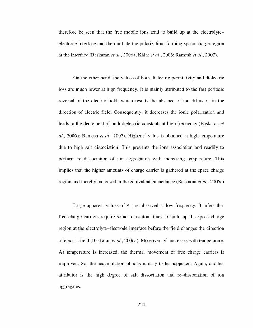
224
therefore be seen that the free mobile ions tend to build up at the electrolyte–
electrode interface and then initiate the polarization, forming space charge region
at the interface (Baskaran et al., 2006a; Khiar et al., 2006; Ramesh et al., 2007).
On the other hand, the values of both dielectric permittivity and dielectric
loss are much lower at high frequency. It is mainly attributed to the fast periodic
reversal of the electric field, which results the absence of ion diffusion in the
direction of electric field. Consequently, it decreases the ionic polarization and
leads to the decrement of both dielectric constants at high frequency (Baskaran et
al., 2006a; Ramesh et al., 2007). Higher 'ε value is obtained at high temperature
due to high salt dissociation. This prevents the ions association and readily to
perform re–dissociation of ion aggregation with increasing temperature. This
implies that the higher amounts of charge carrier is gathered at the space charge
region and thereby increased in the equivalent capacitance (Baskaran et al., 2006a).
Large apparent values of "ε are observed at low frequency. It infers that
free charge carriers require some relaxation times to build up the space charge
region at the electrolyte–electrode interface before the field changes the direction
of electric field (Baskaran et al., 2006a). Moreover, "ε increases with temperature.
As temperature is increased, the thermal movement of free charge carriers is
improved. So, the accumulation of ions is easy to be happened. Again, another
attributor is the high degree of salt dissociation and re–dissociation of ion
aggregates.

225
0
2000
4000
6000
8000
10000
12000
14000
1 1.5 2 2.5 3 3.5 4 4.5 5 5.5 6 6.5
Log [f(Hz)]
�'
303K 313K 323K 333K 343K 353K
Figure 7.6: Typical plot of the variation of real part of dielectric constant ( 'ε ) with frequency for CPE 4 in the temperature range of 303–353 K.
0
500
1000
1500
2000
2500
3000
3500
4000
4500
5000
5500
1 1.5 2 2.5 3 3.5 4 4.5 5 5.5 6 6.5
Log [f(Hz)]
�''
303K 313K 323K 333K 343K 353K
Figure 7.7: Typical plot of the variation of imaginary part of dielectric constant ( ''ε ) with frequency for CPE 4 in the temperature range of 303–353 K.

226
7.5 Dielectric Moduli Studies
The dielectric modulus parameter is well known to represent the bulk
dielectric behavior of the polymer electrolytes because of the elimination of
polarization effect (Ramesh et al., 2007). Real ( 'M ) and imaginary ( "M ) parts of
dielectric moduli as a function of frequency are shown in Figures 7.8 and 7.9,
respectively. These values approach to zero at low frequency and signify the
suppression of electrode polarization effect. The long tail denotes the large extent
of capacitance associated with electrodes (Ramesh et al., 2007). An obvious
observation is examined for real part of dielectric modulus at high frequency. The
dielectric modulus response shows the superposition characteristic in the same
temperature range. This implies the temperature–independent of real dielectric
modulus of CPE 4 at high frequency and suggests that CPE 4 exhibits excellent
electrochemical stability (Suthanthiraraj et al., 2009). Even though well–defined
relaxation peak is not observed in both figures; however it shows the intense
increase at high frequency region. The curve peaks indicate the bulk effect in the
polymer matrix and further infer that the polymer electrolytes are in ionic
conducting mechanism. The intensity of these peaks decreases with increasing
temperature due to the plurality of relaxation mechanism.

227
0.00
0.05
0.10
0.15
0.20
0.25
0.30
0.35
0.40
0.45
0.50
1 1.5 2 2.5 3 3.5 4 4.5 5 5.5 6 6.5Log [f(Hz)]
M'
303K 313K 323K 333K 343K 353K
Figure 7.8: Variation of real modulus ( 'M ) as a function of frequency for CPE 4 in the temperature range of 303–353 K.
0.00
0.05
0.10
0.15
0.20
0.25
1 1.5 2 2.5 3 3.5 4 4.5 5 5.5 6 6.5Log [f(Hz)]
M''
303K 313K 323K 333K 343K 353K
Figure 7.9: Variation of imaginary modulus ( ''M ) as a function of frequency for CPE 4 in the temperature range of 303–353 K.

228
7.6 HATR–FTIR studies
HATR–FTIR spectra of pure SiO2, CPE 1, CPE 3 and CPE 4 are shown in
Figure 7.10(a)–(d). The combination of HATR–FTIR spectra of IL 6, pure SiO2,
CPE 1, CPE 3 and CPE 4 is depicted in Figure 7.11. The HATR–FTIR spectrum
of CPE 4 is discussed in details as it achieves maximum ionic conductivity. All of
the descriptions of the vibrational modes for this polymer electrolyte are tabulated
in Table 7.2. The changes in shift, changes in shape and changes in intensity are
examined in order to confirm the complex mode between SiO2 and polymer matrix.
Regarding to the changes in shift, most of the vibrational modes manifest
downward shifts. The characteristic peaks at 963 cm-1 and 985 cm-1 are defined as
C–O symmetric stretching mode in C–O–C linkage of PMMA and CH2 wagging
mode of PMMA, respectively. For first peak, it shifts from 966 cm-1 to 963 cm-1,
whereas it is shifted from 988 cm-1 for latter peak, asserting the interaction
between PMMA and SiO2. An apparent shift is also observed. The combination of
CH3 asymmetric bending mode of PMMA and C–H stretching mode of CH2 group
of PVC shifts from 1452 cm-1 to 1436 cm-1 and thereby indicates the establishment
of interaction of PMMA, PVC and SiO2.
As explained in ac–impedance studies, the interaction between BmImTFSI
and SiO2 filler disrupts the hydrogen bonding among SiO2 aggregates and this is
being verified in the study. CH3 symmetric stretching mode of BmImTFSI and
CH2 stretching mode of BmImTFSI shift from 1461 cm-1 to 1441 cm-1 and 2963
cm-1 to 2952 cm-1, respectively. C–H vibrational modes for cyclic BmIm+ of

229
BmImTFSI at 3119 cm-1 and 3156 cm-1 are shifted from 3121 cm-1 and 3157 cm-1,
respectively. The shift of S–CH3 bonding mode of TFSI anions from 2880 cm-1 to
2851 cm-1 divulges the interaction between SiO2 and TFSI-. Pure SiO2 illustrates a
broad and sharp peak at 3448 cm-1 and it is assigned as O–H stretching vibrations
of surface hydroxyl group of SiO2. However, it is disappeared in CPE 4 spectrum.
It might be due to the overlapping with N–H stretching mode of BmImTFSI which
located at 3583 cm-1, leading to a formation of a new broad band at 3620 cm-1 in
CPE 4 spectrum. This is reminiscent of the hydrogen bonding between N atom of
TFSI anions and Si–OH of surface hydroxyl group of fumed silica, as shown in
Figure 7.2. On the other hand, the characteristic peak at 700 cm-1 which assigned
as combination of cis wagging mode of PVC and C–H vibrational mode for cyclic
BmIm+ is shifted upward, from 698 cm-1 to 700 cm-1.
Figure 7.10 (a): HATR–FTIR spectrum of pure SiO2.

230
Figure 7.10 (b): HATR–FTIR spectrum of CPE 1.
Figure 7.10 (c): HATR–FTIR spectrum of CPE 3.

231
Figure 7.10 (d): HATR–FTIR spectrum of CPE 4.
Figure 7.11: Combination of HATR–FTIR spectra for (a) IL 6, (b) pure SiO2,
(c) CPE 1, (d) CPE 3 and (e) CPE 4.

232
Descriptions of vibration modes Wavenumber (cm-1)
Reference
Combination of cis C–H wagging mode of PVC and C–H vibrational mode for cyclic BmIm+ of BmImTFSI
698 Achari et al., 2007; Jiang et
al., 2006 Combination of CH2 rocking mode of PVC and S–N stretching mode of LiTFSI
740 Ahmad et al., 2008;
Rajendran et al., 2008
CF3 symmetric bending mode of BmImTFSI 761 Bazito et al., 2007
Combination of C–S and S–N stretching mode of LiTFSI and BmImTFSI
789 Ahmad et al., 2008
Characteristic peak of SiO2 809 Ramesh and Lu, 2008
C–Cl stretching mode of PVC 840 Rajendran et al, 2008
Trans C–H wagging mode of PVC Achari et al., 2007
C–O symmetric stretching mode in C–O–C linkage of PMMA
963 Achari et al., 2007
CH2 wagging mode of PMMA 985 Rajendran et al, 2002
S–N–S asymmetric stretching mode of LiTFSI and BmImTFSI
1055 Ahmad et al., 2008
Combination of C–O–C asymmetric stretching mode of PMMA, C–SO2–N bonding mode of LiTFSI and BmImTFSI and Si–O–Si of SO2
1133 Jiang et al., 2006; Ramesh and Lu, 2008
Combination of CH2 twisting mode of PMMA, CF3 symmetric stretching mode of LiTFSI and C–H vibrational mode for cyclic BmIm+ of BmImTFSI
1176 Achari et al., 2007; Ahmad et al., 2008; Jiang et al.,
2006 N–H stretching mode of BmImTFSI 1226 Bazito et al.,
2007 C–O–C symmetric stretching mode of PMMA 1276 Jiang et al.,
2006 C–SO2 –N bonding mode of LiTFSI and BmImTFSI
1330 Ramesh and Lu, 2008
SO2 asymmetric stretching mode of LiTFSI and BmImTFSI
1349 Ahmad et al., 2008
Combination of CH3 asymmetric bending mode of PMMA, C–H stretching mode of CH2 group of PVC
1436 Rajendran et al, 2008
CH3 symmetric stretching mode of BmImTFSI
1441 Jiang et al., 2006

233
C–C and C–N bending mode of BmImTFSI 1571 Jiang et al., 2006
Combination of C=C stretching mode of PVC and O–H deformation vibrations of surface hydroxyl group of SiO2
1630 Achari et al., 2007
C=O stretching mode of PMMA 1723 Li et al., 2006a
S–CH3 bonding mode of LiTFSI and BmImTFSI
2851 Ramesh and Lu, 2008
CH2 stretching mode of BmImTFSI 2952 Jiang et al., 2006
C–H vibrational mode for cyclic BmIm+ of BmImTFSI
3119, 3156 Jiang et al., 2006
Combination of N–H stretching mode of BmImTFSI and O–H stretching vibrations of surface hydroxyl group of SiO2
3620 Jiang et al., 2006
Table 7.2: Assignments of vibrational modes of PMMA, PVC, LiTFSI, BmImTFSI and SiO2 for CPE 4.
Figure 7.12 illustrates the evidence of change in intensity of C=O
stretching mode of PMMA. The intensity of peak reduces by 23.25 %, from 56.43
% to 33.18 %, in transmittance mode. In addition, it shifts downward slightly, that
is from 1725 cm-1 to 1723 cm-1. Similar observation is attained for C–O–C
symmetric stretching mode at 1276 cm-1. This characteristic peak is shifted from
1281 cm-1 to 1276 cm-1 and its intensity is decreased by 3.57 % in transmittance
mode, from 8.57 % to 5 %. This signifies the interaction of PMMA with SiO2 and
thereby initiates the ion transportation by decoupling the Li+ from the coordination
bond with C=O of PMMA. Visible changes in intensity are noticed at 1055 cm-1
and 1571 cm-1. First peak is assigned as S–N–S asymmetric stretching mode of
LiTFSI and BmImTFSI. In terms of peak intensity, it decreases by 30.32 % in
transmittance mode, from 47.14 % to 16.82 %. It has also been shifted from 1053
cm-1. These changes further reveal the hydrogen bonding between N atoms of
TFSI anions and Si–OH on the surface of nano–sized filler. Combination of C–C

234
and C–N bending mode of BmImTFSI shifts from 1574 cm-1 to 1571 cm-1. Around
15.06 % of decrease in intensity is attained and it is shifted from 16.42 % to 1.36
%, in transmittance mode. Even though the wavenumber of combination of C–S
and S–N stretching mode of LiTFSI and BmImTFSI still remains at 789 cm-1,
however, the peak intensity reduces by 22.59 %, from 27.14 % to 4.55 % in
transmittance mode.
Figure 7.12: The comparison of change in intensity of C=O stretching mode
of PMMA in (a) IL 6and (b) CPE 4.
Some facts of changes in shape have been shown in comparing IL 6 and
CPE 4. The assignment for the characteristic peak at 738 cm-1 is combination of
CH2 rocking mode of PVC and S–N stretching of LiTFSI. On the other hand, the
CF3 symmetric bending mode of BmImTFSI is placed at 748 cm-1. Both of these
peaks demonstrate downward shifts. The first peak shifts from 740 cm-1, whereas
761 cm-1 is for latter peak. These two peaks possess some obvious changes in
shape that is from a sharp peak with shoulder to two weak peaks, revealing the

235
interaction between PVC, LiTFSI, BmImTFSI and SiO2. C–Cl stretching mode of
PVC is not only shifted from 845 cm-1 to 840 cm-1, but it also has been changed
from a sharp peak to a weak peak. A new resolved peak is appeared at 809 cm-1
and assigned as characteristic peak of SiO2, as highlighted in Figure 7.11 (c). A
noticeable change is observed for C=C stretching mode of PVC at the
wavenumber of 1630 cm-1. A medium sharp peak has been changed to a less
intense broad band. It might be due to the overlapping effect of O–H deformation
vibrations of surface hydroxyl group of SiO2 with this stretching mode. This broad
band is further implied the lower crystallinity of sample with addition of 8 wt% of
SiO2 as a broad peak is an indicative of low crystalline structure of polymer
electrolyte (Suthanthiraraj et al., 2009).
The bands in the wavenumber range of 1400 cm-1–1100 cm-1 are explored
in order to investigate the ion aggregation further. Two important peaks are
obtained in the region of 1200 cm-1–1100 cm-1. The first peak is assigned as
combination of C–O–C asymmetric stretching mode of PMMA, C–SO2–N
bonding mode of LiTFSI and BmImTFSI at 1133 cm-1, whereas combination of
CH2 twisting mode of PMMA, CF3 symmetric stretching mode of LiTFSI and C–H
vibrational mode for cyclic BmIm+ of BmImTFSI is assigned at 1176 cm-1. The
downward shift of first peak from 1140 cm-1 to 1133 cm-1, might be due to the
contribution of Si–O–Si bonding of SiO2 at 1100 cm-1. This indicates that the TFSI
anions favor to interact with silica and thus promote the decoupling of Li+ and
BmIm+ from doping salt and ionic liquid. Eventually, it induces to higher ionic
conductivity. On the other hand, the second peak exhibits upward shift from 1168

236
cm-1 to 1176 cm-1. Based on these two peaks, the obvious change in shape is
obtained as shown in Figure 7.13. This figure illustrates that a broad band is
changed to two sharp peaks.
The HATR–FTIR spectra of CPE 1, CPE 3 and CPE 4 are compared in
order to prove the highest ionic conductivity of CPE 4. At 809 cm-1, the
characteristic peak of SiO2 is absent in CPE 3 and CPE 4 spectrum. Two weak
peaks should be shown in the region 1500 cm-1–1400 cm-1. However, there is only
a peak has been shown in this range for CPE 1. The peak which designated as
combination of CH3 asymmetric bending mode of PMMA, C–H stretching mode
of CH2 group of PVC is absent. On the other hand, a weak peak which assigned as
combination of cis C–H wagging mode of PVC and C–H vibrational mode for
cyclic BmIm+ of BmImTFSI is also absent in CPE 3 spectrum. Other assignments
are present in both spectra. As shown in Figure 7.11, the intensity of peak is
increased as increases amount of SiO2 by comparing CPE 1, CPE 3 and CPE 4.
This suggests the formation of grain boundaries between the aggregates with
excessive SiO2 nano–particles and contributes to higher polarity of the polymer
matrix. It can therefore be seen that higher bond energy is obtained and hence
forms more intense absorption peak in this region.

237
Figure 7.13: The comparison of change in shape of the vibrational modes in
the wavenumber region of 1200 cm-1–1000 cm-1 for (a) IL 6 and (b) CPE 4.
Viscosity is another attributor for the increase in ionic conductivity for
CPE 4, as explained in ac–impedance study. This factor can be proven in HATR–
FTIR study in the wavenumber region of 1400 cm-1–1100 cm-1. Two peaks are
observed in this range. First peak at 1330 cm-1 is assigned as C–SO2–N bonding
mode of LiTFSI and BmImTFSI, whereas SO2 asymmetric stretching mode of
LiTFSI and BmImTFSI is for the characteristic peak at 1349 cm-1. The
wavenumber for first peak remains the same, however, the latter peak shifts from
1346 cm-1 to 1349 cm-1, asserting the TFSI anions with SiO2. As shown in Figure

238
7.11, the intensity of peak decreases with increasing SiO2 concentration. It can
therefore be concluded that CPE 4 has lowest viscosity. As increases the
composition of SiO2, the interaction between BmImTFSI and polymer matrix
becomes lesser as the interaction between BmImTFSI and SiO2 is more favorable.
As a result, the entanglements within polymer matrix are lesser and lead to lower
viscosity of polymer electrolytes.
7.7 XRD Studies
XRD analysis has been performed, and their respective diffraction patterns
of IL 6, CPE 1, CPE 3 and CPE 4 are shown in Figures 7.14 (a)–(d). Apparently,
the change in shape is observed, from a broad peak with a shoulder to a new broad
peak upon inclusion of SiO2, as shown in Figure 7.14. The disappearance of
shoulder is insinuative of an increase in amorphous behavior of polymer
electrolytes, which is primarily due to the formation of polymeric network. It
deteriorates the ordered arrangement of polymer matrix, promotes the segmental
mobility of polymer chain and favors the ionic transportation as discussed in ionic
conductivity studies. The peak is slightly shifted upon dispersion of SiO2. The
broad peak at Bragg angle of 2�=18.5° is shifted to 2�=18°, indicating the
complexation between the SiO2 and polymer matrix (Kumar et al., 2007). Another
noticeable observation is obtained for CPE 3 and CPE 4. The peak of CPE 4 is
much broader than CPE 3 infers that the CPE 4 has higher amorphous behavior
than CPE 3, ultimately leads to improvement of the ion diffusivity in accordance

239
with higher ionic conductivity.
In addition, coherent length study is carried out to examine the crystallite
size in the polymer matrix. Based on Debye–Scherrer equation, the broader the
diffraction peak width, the shorter of crystallite size is, contributing to the lower
crystallinity in the polymer matrix (Aravindan et al., 2009). Therefore, the
coherent length decreases with increasing SiO2 amount, as illustrated in Figure
7.15. As explained above, inclusion of SiO2 forms three–dimensional network
among aggregates and contributes to the distortion of the arrangement of polymer
matrix. Hence, it leads to development of amorphous region. In general, the
segmental mobility and flexibility of polymer backbone are enhanced in
amorphous phase and this promotes ionic transportation, reflecting the higher ionic
conductivity.
0 10 20 30 40 50 60 70 802� (°)
Inte
nsity
(a.u
)
Figure 7.14: XRD patterns of (a) IL 6, (b) CPE 1, (c) CPE 3 and (d) CPE 4.
(a)
(b)
(c)
(d)

240
0.67
0.430.46
0.52
0.40
0.45
0.50
0.55
0.60
0.65
0.70
0 2 4 6 8Percentage of SiO2 (% wt)
Coh
eren
ce le
ngth
(Å)
Figure 7.15: Variation of coherence length at ambient temperature with
respect to different mole fraction of SiO2 in the nano–composite polymer electrolytes at 2�≈ 18°C.
7.8 SEM Studies
The morphologies of all CPEs are illustrated in Figure 7.16 (a)–(c). Indeed,
the morphology of polymer electrolytes is totally altered upon addition of SiO2.
The spherulites in the IL 6 are suddenly disappeared and the appearances of CPEs
are being transformed into a wavy type surface morphology. This wavy type
appearance reveals the pre–dominant amorphous region in the polymer electrolytes
by destroying the crystallinity portion among the polymer matrix, along with
further disruption of interaction among the polymer side chain. The blackish
cavities infer the presence of ion transfer in the polymer electrolytes, as shown in
Figures 7.16 (a)–(c). As discussed earlier, the occurrence of black cavity is an

241
evidence for ionic transportation in the polymer matrix. Comparing CPE 1 and
CPE 3, CPE 3 has more black cavities than CPE 1. Therefore, it could be
concluded that the ion hopping mechanism of CPE 3 is more favorable than CPE 1.
It is mainly due to SiO2 is in excess mode for CPE 3 and hence promotes the ionic
migration in the nano–composite polymer electrolyte. In contrast, the ion mobility
of CPE 1 does not reaches the desired level as little amount of SiO2 is added into
the polymer electrolyte.
Some fine and tiny white sphericals are obtained in Figure 7.16 (c) is
evocative of the dispersion of SiO2 nano–particles. The diameter of the sphericals
is within the range of 0.1 �m instead of nano–sized. This reveals the aggregations
among the nano–sized particles via hydrogen bonding on the surface of silica
atoms. Figure 7.16 (c) shows that the size of cavities is also distinctively increased.
Typically, it might be due to the formation of three–dimensional network as a
result of the hydrogen bonding among aggregates. This creates some entrapments
within polymer matrix. So, large volumes of filler and gel electrolytes are being
entrapped in the cavities and hence, it accounts for the highest ionic conductivity
by enhancing the ionic migration among the polymer matrix.

242
Figure 7.16 (a): SEM images of CPE 1.
Figure 7.16 (b): SEM images of CPE 3.

243
Figure 7.16 (c): SEM images of CPE 4.
7.9 DSC Studies
DSC traces of all the CPEs samples are depicted in Figure 7.17 and
tabulated in Table 7.3. Same trends of all DSC profiles are clearly observed.
Initially, a small change in heat flow from exothermic reaction to endothermic
reaction and it is commonly assigned as glass transition temperature ( gT ). A
gradual decrease in heat flow of polymer matrix is tagged along, up to above 151
°C. A weak endothermic peak is then observed and it is known as melting point of
the polymer electrolytes, mT . Two consecutive peaks are observed thereafter and
they are defined as decomposition temperatures of polymer electrolytes, dT . The

244
first endothermic decomposition peak is originated from the dehydrochlorination
of PVC, as explained in section 4.10 (Ahmad et al., 2006b). On the other hand, the
second endothermic peak is ascribed to the breakdown of unsaturated group of
PMMA such as carbonyl functional group and degradation of PVC (Ahmad et al.,
2006a).
A slight downward shift in gT from 112 °C for IL 6 to 109 °C for CPE 4
reveals that the amorphous proportion increases with the mass fraction of fumed
silica. The shift towards lower temperature indicates the softening effect in the
polymer matrix and thus enhances the segmental motion of polymer backbone
(Ramesh and Arof, 2001b). This suggests that the formation of three–dimensional
network among aggregates has interrupted the coordination bond in the polymer
matrix and formed more flexible polymer backbone. It can therefore be seen that
the ionic migration is enhanced after impregnation of SiO2 by weakening the
coordination bonding within the polymer matrix.
mT also exhibits same feature as gT . As quantity of SiO2 increases, it is
further decreased. mT decreases from 157 °C (IL 6) to 152 °C (CPE 4) as shown in
Figure 7.17. Indeed, more asymmetric endothermic meting peaks are being
depicted in the DSC thermogram. This divulges the decrease in crystalline degree
or increase in amorphous region of both polymer electrolytes (Pandey et al., 2009).
The amorphous nature of polymer electrolytes accelerates the segmental mobility
and ionic transportation in the electrolytes, which results high ionic conductivity.

245
Lower mT evolves with smaller peak area (or known as lower of heat of fusion) is
illustrated with increasing the mass fraction of fumed silica. This further indicates
the increase in amorphous proportion in polymer electrolytes. As explained,
formation of three–dimensional network disrupts the ordered arrangement within
polymer matrix and forms more flexible backbone and voids within the polymer
matrix. As a result, it improves the ion hopping process. This result is in good
agreement with XRD and SEM analyses.
Two endothermic decomposition peaks are sequentially observed. An
apparent characteristic is obtained for dT : the decomposition temperatures shift
upward upon enclosure of SiO2. A gradual increase from 376 °C for SiO2–free
polymer electrolyte to 379 °C for CPE 4 is obtained for first decomposition
temperature. Nevertheless, a smaller deviation of second decomposition
temperature is further achieved, that is from 399 °C (without SiO2 dispersion) until
400 °C (CPE 1, CPE 3 and CPE 4). Upon inclusion of SiO2, the decomposition
temperatures are increased. It is mainly ascribed to the formation of hydrogen
bonding among its aggregates via chemi–adsorptions of Si–OH on the hydroxyl
surface of silica atoms from SiO2. Development of network is more preferred when
the sufficient amount of SiO2 is thoroughly dispersed the polymer matrix. So, it
requires more energy to break the hydrogen bonds within the polymeric network.
The highest decomposition temperatures of CPE 4 imply that the thermal property
of the polymer matrix is increased. Therefore, CPE 4 is the better choice as
composite polymer electrolyte.

246
0 50 100 150 200 250 300 350 400 450
Temperature (°C)
Hea
t flo
w (m
W)
Figure 7.17: DSC thermograms of (a) IL 6, (b) CPE 1, (c) CPE 3 and (d)
CPE 4.
DSC measurements Designations gT (°C) mT (°C) dT (°C)
IL 6 112.50 157.30 375.66, 399.40 CPE 1 111.50 154.60 377.40, 399.80 CPE 3 110.40 153.80 378.10, 399.80 CPE 4 109.50 151.90 379.20, 399.90
Table 7.3: DSC profiles of PMMA–PVC–LiTFSI–BmImTFSI based nano–composite polymer electrolytes.
7.10 TGA Studies
TGA thermograms are shown in Figure 7.18, three stages are clearly
observed for the degradation curves. Initial weight loss of 5 % at 137 °C, 3 % at
146 °C, 5 % at 166 °C and 1% at 178 °C are observed for IL 6, CPE 1, CPE 3 and
CPE 4, respectively. The initial weight loss is generally ascribed to the evaporation
of THF solvent, elimination of impurities especially fluorine compound and
(a) (b)
(c)
(d)
endo
exo

247
dehydration of entrapped moisture (Stephan et al., 2002). Beyond the first mass
loss, it follows by a constant weight. After that, second and third weight losses
exist in the TGA thermogram. Second weight loss is mostly attributed to the
unzipping process in the temperature regime. This process initiates many
degradation reactions such as random chain scission reaction, depolymerization,
intra–molecular transfer reaction and inter–molecular transfer reaction as well as
polymer fragments. Therefore, volatilization of the monomer and oligomers which
chemi–adsorbed onto the polymer matrix is occurred in this temperature regime.
Eventually, the weight loss is significantly decreased (Ahmad et al., 2007).
Elimination of HCl compounds from the dehydrochlorination reaction is another
contributor, as proven in DSC thermograms. Around 17 % of second mass loss is
observed for IL 6, starting from 255 °C to 355 °C, however, this respective weight
loss decreases further by dispersing nano–sized SiO2. CPE 1 and CPE 3 exhibit the
mass losses of 14 % and 15 % with correspond of theirs’ temperature ranges of
274 °C–384 °C and 284 °C–364 °C. Excellent thermal stability is revealed by CPE
4, 13 % of weight loss is observed, whereby the degradation temperature starts
from 277 °C and end up at 357 °C.
After second weight loss, a gradual mass loss is observed thereafter. This
particular weight loss is related to degradation of unsaturated groups of PMMA
and decomposition of PVC, as verified in DSC analysis. In this stage, IL 6
displays around 12 % of weight loss at 385 °C with a residual mass of 66 %,
weight losses of CPEs decreases enormously by incorporating fumed silica. CPE 1
and CPE 3 reveal 12 % and 7 % of mass losses, along with 71 % and 73 % residue

248
at 384 °C, respectively. Nevertheless, CPE 4 illustrates around 7 % weight loss
with residual mass of 79 % at 387 °C. This might be due to inclusion of high
amount of fumed silica in the polymer matrix. It leads to tight bonding within the
polymer segments. Therefore, less volatilization is occurred (Rajendran et al.,
2002). A complete decomposition of all the electrolytes has been verified by
showing a stable mass thereafter. Among all the polymer electrolytes, CPE 4
discloses the excellent thermal stability, where the stability is up to 277 °C.
60
65
70
75
80
85
90
95
100
105
0 50 100 150 200 250 300 350 400 450
Temperature (°C)
Wei
ght (
%)
IL 6 CPE 1 CPE 3 CPE 4
Figure 7.18: Thermogravimetric analysis of IL 6, CPE 1, CPE 3 and CPE 4.
7.11 Amplitude Sweep
The amplitude sweeps of IL 6 and SiO2–based gel polymer electrolytes are
shown in Figure 7.19, on logarithm scale. For all the samples, the 'G values are
higher than ''G in the strain regime, inferring the solid properties of all the
65.68%
72.78% 78.77%
71.06%

249
samples. The absence of crossover point of 'G and ''G denotes that the behavioral
transition of the polymer electrolytes did not occurs within the range (Fonseca et
al., 2009). The trend of plots is similar as the previous polymer system. First,
slight decreases in 'G and ''G are observed for initial deformation. It thus
followed by a constant LVE range, and eventually, the abrupt decrease is attained
at high imposed deformation. As can be seen, CPE 1 shows the narrowest LVE
range among all the composite polymer electrolytes, indicating the least stable of
the sample.
At 0.001 % of strain, the values of 'G and ''G are substantially increased
upon addition of fumed silica. It is suggestive of establishment of three–
dimensional network among the SiO2 particles due to the formation of silanol (Si–
OH) linkages on the surface of silicon atom of SiO2 through Van der waals
attractive force and hydrogen bonding as it is a hydrophilic compound (Ahmad et
al., 2005; Ahmad et al., 2006a; Li et al., 2006b). As a theoretical result, more
physical reticulate structures would be formed as increases in SiO2 composition,
which results the increment of 'G and ''G values. However, the result is against
the theory.
This observation might be due to the formation of space charge layers as a
result of repulsion forces between the SiO2 particles. At high SiO2 content, these
space charge layers induce to the longer distances between the SiO2 grains and
further weaken the physical networks. Additionally, the network is also destroyed
with the inclusion of ionic liquid. As shown in Figure 7.19, the TFSI anions prefer
250
to form hydrogen bond with the network between SiO2 grains and thus weaken the
interaction among the aggregates. Among all the composite polymer electrolytes,
CPE 4 exhibits the lowest values of 'G and ''G , inferring the lowest viscosity of
CPE 4.
0.1
1
10
100
1000
0.001 0.01 0.1 1 10 100 1000Strain (%)
G' a
nd G
'' (P
as)
IL 6(G') IL 6(G'') CPE 1(G') CPE 1(G'') CPE 3(G')CPE 3(G'') CPE 4(G') CPE 4(G'')
Figure 7.19: Amplitude sweeps of IL 6 and SiO2–based gel polymer
electrolytes.
7.12 Oscillatory Stress Sweep
The oscillatory shear curves of IL 6 and SiO2–based gel polymer
electrolytes are exemplified in Figure 7.20, on logarithm scale. The higher values
of 'G than ''G proposes the solid nature of the samples within the range of shear
stress (Li et al., 2006b). The behavioral transition is not being occurred as the flow
point is absent in all the samples (Fonseca et al., 2009). Three distinct stages are

251
observed and the trend of plots is discussed in previous section. Upon
incorporation of SiO2, the polymer electrolytes normally use larger shear stress to
disrupt the bonds and linkages due to the formation of three–dimensional network.
As proven in the figure, CPE 1 and CPE 3 are not easily to be distorted as they
need high shear stress to rupture the polymeric systems. The main attributor of this
observation is the silanol linkages among the silica particles and it favors the
three–dimensional network in the complex. As a result, more energy is required to
destroy this entanglement.
Among all the CPEs, the increase sequence in the required amount of shear
stress for the initial deformation is in this order: CPE 4 < CPE 3 < CPE 1. The
apparent decrease in initial shear stress is attained as increases the SiO2 loadings.
Excessive nano–SiO2 particles cause the repulsion among the aggregates and
hence weaken the interactions within the polymer matrix further, which in turn to
the lower values of 'G and ''G . In addition, CPE 1 imparts lower stability at high
shear stress by showing the rapid decreases in 'G and ''G . In contrast, CPE 3 and
CPE 4 exhibit higher stability even though they depict lower values of both moduli.
Therefore, the solid–like behavior of polymer electrolytes can be improved by
doping more SiO2 concentration at high deformation.

252
0.1
1
10
100
1000
0.00001 0.0001 0.001 0.01 0.1 1 10 100Shear stress (Pa)
G' a
nd G
'' (P
as)
IL 6(G') IL 6(G'') CPE 1(G') CPE 1(G'') CPE 3(G')CPE 3(G'') CPE 4(G') CPE 4(G'')
Figure 7.20: Oscillatory shear sweeps of IL 6 and SiO2–based gel polymer
electrolytes.
7.13 Oscillatory Frequency Sweep
The typical frequency sweeps of IL 6 and SiO2–based gel polymer
electrolytes are shown in Figure 7.21. The absence of ''G profile confirms once
again the elastic solid–like properties of CPEs in the frequency range. The effect
of incorporation with SiO2 is not apparently observed as the 'G values are almost
the same in the frequency regime. It might be due to the low doping amount of
SiO2 and it induces to the futile effect on the structural stability of polymer
electrolytes. For IL 6 and all CPEs, there is an abrupt decrease in 'G at low
frequency, as illustrated in Figure 7.21. When the deformation occurs for longer
time at low frequency, the relaxation time becomes longer and contributes to the
slippage of entanglements. This slippage reduces the ability for storing the

253
imposed energy and hence decreases the solid behavior of sample, indicating the
low structural stability of the polymer system at low frequency.
In contrast, at higher frequency, the structural stability of polymer
electrolytes is improved as the high value of 'G is shown in Figure 7.21. Again, it
is primarily attributed to the low relaxation time and then leads to insufficient time
for slippage mechanism. Therefore, the structural strength of polymer electrolytes
at high frequency is better than at low frequency. Since all the plots show the
comparable values within the range, it can therefore be concluded that the addition
of SiO2 is not a promising candidate to improve the stability of polymer
electrolytes.
10000
100000
0.01 0.1Angular frequency, � (rad/s)
G' a
nd G
'' (P
as)
IL 6 CPE 1 CPE 3 CPE 4
Figure 7.21: Frequency sweeps of IL 6 and SiO2–based gel polymer electrolytes.

254
7.14 Viscosity Studies
Figure 7.22 shows the typical viscosity profile as a function of shear rate
with various mass fractions of fumed silica. Non–newtonian nature has been
shown in IL 6 and CPEs as the viscosity exhibits the linear relationship with
respect to shear rate (Ahmad et al., 2005). When the sample is less deformed, the
value of viscosity is still high at lower shear rate. This is due to the initial
deformation and the sample still maintains its elastic properties by forming the
polymer network among the aggregates via silanol linkage. However, the viscosity
decreases monotonically with increasing the shear rate, revealing the shear
thinning properties. It is because the network among the SiO2 particles is destroyed
by shear. At high shear rate, the viscosity and shear thinning rate for IL 6 and
CPEs are quite similar due to the preferential orientation of the silanol linkage
parallel to the flow direction (Ahmad et al., 2005).
In principle, the viscosity of sample should be increases with shear rate due
to the formation of three–dimensional network among the aggregates through the
silanol linkage, as explained in previous amplitude sweep and oscillatory shear
sweep studies. However, at low shear rate (0.1 s-1), the viscosity is reduced upon
addition of fumed silica. The perspective on this result is because of the presence
of ionic liquid. The ionic liquid contributes the plasticizing effect and thus
weakens the intertwined network linkages among the aggregates. The viscosity of
CPEs decreases with increasing the content of SiO2. At high SiO2 composition,
SiO2 nano–particles are in excess mode. Excessive SiO2 causes the repulsion

255
forces between the aggregates and therefore weakens the interaction between
three–dimensional networks by producing longer distance between the aggregates.
As a result, CPEs imparts lower viscosity.
0.1
1
10
100
1000
10000
0.1 1 10 100Shear rate (1/s)
Visc
osity
, � (P
as)
IL 6 CPE 1 CPE 3 CPE 4
Figure 7.22: Typical viscosity curve of IL 6 and SiO2–based gel polymer electrolytes.
7.15 Summary
Nano–composite polymer electrolytes with different ratio of fumed silica
were prepared by solution casting technique. Among all the samples, CPE 4 (8
wt% of SiO2) is a feasible candidate. Maximum ionic conductivity of
(4.11±0.01)×10-3 Scm-1 is achieved by CPE 4 due to the formation of an effective
conducting pathway between the grain boundaries. The conductivity increases

256
with frequency, up to an optimum level. Beyond this region, the decrease in
conductivity is perceived. At low frequency, slow periodic reversal causes the
accumulation of ions and hence decreases the ion transport in the polymer matrix
which in accordance with lower conductivity. Both of dielectric permittivity and
dielectric loss decrease with frequency. Electrode polarization due to the
accumulation of ions is the main attributor. There is no ion diffusion in the
direction of electric field at high frequency due to the fast periodic reversal of
electric field. In order to study the bulk dielectric response of polymer electrolytes,
the dielectric modulus which mask the polarization effect is investigated. No
evident relaxation peak is observed in both real and imaginary parts of dielectric
moduli. HATR–FTIR study is employed to study the structural of polymer
electrolytes and thus verified the complexation between fumed silica and polymer
blends.
In temperature dependence–ionic conductivity studies, CPE 4 achieves the
highest ionic conductivity of (8.26±0.02) mScm-1 at 80 °C with stability up to 277
°C. CPEs exhibit Arrhenius behavior within the temperature range. Arrhenius
relationship reflects the ion hopping mechanism at elevated temperature. On the
other hand, XRD and coherent length studies prove the highest amorphous region
of the CPE 4. Enhancement in amorphous proportion and ionic mobility in the
polymer matrices are further proven in the SEM morphologies. DSC and TGA
studies imply the improved thermal stability nano–composite polymer electrolytes
as increases in filler loadings. Decrease in gT and mT implies the enhancement of

257
flexibility and amorphous degree of polymer electrolytes, respectively. Significant
decrease in weight loss indicates the excellent thermal properties of composite
polymer electrolytes upon heating to 450 °C.
The elastic solid–like properties of CPEs have been found out in the
amplitude sweep and oscillatory shear sweep studies, as the value of 'G is higher
than ''G . In amplitude sweep, both of 'G and ''G decrease with fumed silica
composition, revealing the gel–like appearance of polymer electrolytes with low
mechanical stability. The samples still remain in gel–like behavior due to the
strong plasticizing effect of ionic liquid. LVE range becomes wider with
increasing fumed silica content and indicates the better stability of these polymer
electrolytes. In addition, the low mechanical properties of the samples are also
shown in oscillatory shear sweep by showing the lower value of starting point of
shear stress. In frequency sweep, ''G is absent and further implies the solid nature
of CPEs. At low frequency, 'G shows lower value due to the longer relaxation
time, which in turn to the slippage of the polymer chain. Therefore, the structural
stability is reduced at low frequency. In contrast, the structural stability is
improved at the short–term of deformation. It is mainly attributed to the declined
relaxation time. Shear–thinning properties of CPEs were observed in viscosity
curve with respect to the shear rate. Under shear, the viscosity is decreased due to
interruption of the weak physical and chemical bonds within the polymer matrix.

258
7.16 Summary of Four Systems on Room Temperature–Ionic Conductivity
Study
Figure 7.23 shows the comparisons of the ionic conductivity for the highest
ionic conducting samples in the polymer blend electrolyte system at room
temperature. As explained in sections 3.2.1 and 3.2.2, 10 wt% of LiTFSI is fixed
in first system, whereas the ratio of PMMA–PVC polymer blends to salt is varied
in second system. Based on the results obtained in Chapter 4, the highest ionic
conductivity of 1.60×10⁻⁸ Scm-1 is reached in the first system. On the contrary,
inclusion of 30 wt% of LiTFSI achieves the maximum ionic conductivity of
1.11 × 10⁻⁶ Scm-1, as explained in Chapter 5. By comparing first system with
second system, the ionic conductivity increases with the mass fraction of lithium
salt. It is mainly ascribed to the increase in the amount of charge carriers (Li+) by
doping LiTFSI further. Therefore, it promotes more ionic hopping mechanism
within the polymer matrix and then raises the ionic conductivity.
In third polymer blend electrolyte system, the ionic conductivity increases
drastically upon adulteration of BmImTFSI ionic liquid. Strong plasticizing effect
of ionic liquid is the main attributor. This effect would soften the polymer
backbone and thus enhance the segmental mobility of polymeric chain, favoring
the ionic transportation which in accordance with high ionic conductivity. Doping
of ionic liquid also weakens the interaction with the polymer matrix and initiates
the decoupling of ions by reducing the solvation of Li+. As a result, the ionic
migration is favored due to its high self–dissociating behavior. The ionic

259
conductivity increases by one order of magnitude upon addition of 8 wt% of
fumed silica onto third system. The ionic conductivity of 4.11 mScm-1 is achieved.
The enhancement of ionic conductivity is suggestive of formation of nano–sized
filler grain boundary. A continuous interpenetrating conducting pathway between
the silica grains in the inter–particles region is generated as the particles are getting
closer to each other. This assists in ionic hopping mechanism and hence leads to
the high ionic conductivity.
-8
-7
-6
-5
-4
-3
-2
First system Second system Third system Fourth system
Systems
Log
con
duct
ivity
, log
[� (
Scm-1
)]
Figure 7.23: Variation of log conductivity, log � of the highest ionic conducting samples in the particular system at ambient temperature.

260
CHAPTER 8
CONCLUSION
Four polymer electrolyte systems were prepared by solution casting
technique. PMMA and PVC were used as host polymers with LiTFSI as doping
salt. Additives such as BmImTFSI ionic liquid and nano–sized inorganic filler,
SiO2 were employed. PMMA (70 wt%) blended with PVC (30 wt%) based
polymer electrolyte was a promising candidate. The highest ionic conductivity
obtained was 1.60 × 10⁻⁸ Scm-1 at ambient temperature. Maximum ionic
conductivity of 1.11×10⁻⁶ Scm-1 was achieved at room temperature with addition
of 30 wt% LiTFSI salt. Ionic liquid was incorporated in this polymer blend
electrolytes to improve the ionic conductivity. The ambient temperature–ionic
conductivity of gel polymer electrolytes enhanced to a maximum value of
1.64 × 10⁻⁴ Scm-1 upon addition of 60 wt% BmImTFSI. The ionic conductivity
increased by two orders of magnitude. The dispersion of 8 wt% of SiO2 (denoted
as CPE 4) was achieved the highest ionic conductivity of 4.11 mScm-1 at room
temperature.
The ionic conductivities of all the samples increased with temperature. It
disclosed the Arrhenius behavior and thus further indicated the ion hopping
mechanism. The dielectric behavior was analyzed using dielectric permittivity and
dielectric modulus of the samples. In frequency dependence study, it obeyed
Jonscher’ s universal law and further proven the hopping process between the

261
charge carriers in the polymer matrix. Non–Debye characteristic was divulged in
dielectric relaxation study. In order to study the bulk dielectric response of
polymer electrolytes, the dielectric modulus which masks the polarization effect
was investigated. In addition, horizontal attenuated total reflectance–Fourier
Transform infrared (HATR–FTIR) spectroscopy indicated the complexation of the
materials in the polymer electrolytes based on the changes in peak shifting,
intensity, shape and formation of new peaks.
X–ray diffraction (XRD) studies implied the higher degree of amorphous
nature of the polymer electrolytes by reducing the intensity of characteristic peaks.
The higher amorphous region is further verified in coherence length study. SEM is
used to investigate the morphology of the samples. By analyzing the SEM images,
the higher porosity revealed the improved ionic migration in the sample.
Entrapments of ionic liquid into the polymer matrix were verified through the
images. DSC studies inferred the improved thermal properties of samples. TGA
asserted the excellent thermal stability of the polymer electrolyte where their
stability is up to 200 °C. Rheological studies revealed the solid and elastic
properties through amplitude sweep and oscillatory shear sweep studies, as the
values of 'G are much higher than ''G . Elastic property of polymer electrolytes
became lesser when the deformation takes place for a prolonged time at low
frequency. In the typical viscosity curves, shear–thinning properties of samples
were observed. CPE 4 is a promising candidate as polymer electrolyte and is
greatly preferred in lithium ion polymer batteries as it shows the excellent thermal
stability, where the stability is up to 277 °C.

262
For further study, liquid crystal will be added as additive into this polymer
blend electrolytes in order to improve the ionic conductivity and overall
performances. Doping of liquid crystal will lead to the formation of liquid crystal
polymer electrolytes. In addition, ionic liquid and nano–sized filler would be
synthesized and then used as additives in the polymer blend electrolytes. The
comparisons between synthesized and commercial additives would be made. The
fabrication of lithium ion rechargeable battery will also be done by using the
highest ionic conducting sample. The overall electrical and electrochemical
performances of the cell will be studied and analyzed in various aspects such as
the cost effectiveness of the cell, charge capacity, discharge capacity and
Coulombic efficiency. The results will be validated with commercial polymer
battery.

263
LIST OF REFERENCES
Achari, V.B., Reddy, T.J.R., Sharma, A.K. & Rao, V.V.R.N. (2007). Electrical, optical, and structural characterization of polymer blend (PVC/PMMA) electrolyte films. Ionics, 13, 349–354.
Adebahr, J., Byrne, N., Forsyth, M., MacFarlane, D.R. & Jacobsson, P. (2003).
Enhancement of ion dynamics in PMMA–based gels with addition of TiO2 nano–particles. Electrochimica Acta, 48, 2099–2103.
Ahmad, S., Ahmad, S. & Agnihotry S.A. (2005). Nanocomposite electrolytes with
fumed silica in poly(methyl methacrylate): thermal, rheological and conductivity studies. Journal of Power Sources, 140, 151–156.
Ahmad, S., Bohidar, H.B., Ahmad, S. & Agnihotry, S.A. (2006a). Role of fumed
silica on ion conduction and rheology in nanocomposite polymeric electrolytes. Polymer, 47, 3583–3590.
Ahmad, S., Saxena, T.K., Ahmad, S. & Agnihotry, S. A. (2006b). The effect of
nanosized TiO2 addition on poly(methylmethacrylate) based polymer electrolytes. Journal of Power Sources, 159, 205–209.
Ahmad, S., Deepa, M. & Agnihotry, S.A. (2008). Effect of salts on the fumed
silica–based composite polymer electrolytes. Solar Energy Materials and Solar Cells, 92, 184–189.
Ahmad, S. & Agnihotry, S.A. (2009). Effect of nano �–Al2O3 addition on ion
dynamics in polymer electrolytes. Current Applied Physics, 9, 108–114. Ahmad, Z., Al–Awadi, N.A. & Al–Sagheer, F. (2007). Morphology, thermal
stability and visco–elastic properties of polystyrene–poly(vinyl chloride) blends. Polymer Degradation and Stability, 92, 1025–1033.
Ali, A.M.M., Yahya, M.Z.A., Bahron, H., Subban, R.H.Y., Harun, M.K. and Atan,
I. (2007). Impedance studies on plasticized PMMA–LiX [X: CF3SO3−,
N(CF3SO2)2−] polymer electrolytes. Materials Letters, 61, 2026–2029.

264
Almond, D.P., West, A.R. & Grant, R. J. (1982). Temperature dependence of the A.C. conductivity of Na �–alumina. Solid State Communications, 44, 1277–1280.
Arof, A.K. and Ramesh, S. (2000). Electrical conductivity studies of
poly(vinylchloride) based electrolytes with double salt system. Solid State Ionics, 136–137, 1197–1200.
Aravindan, V., Lakshmi, C. & Vickraman, P. (2009). Investigations on Na+ ion
conducting polyvinylidenefluoride–co–hexafluoropropylene / poly ethylmethacrylate blend polymer electrolytes. Current Applied Physics, 9, 1106–1111.
Barsoukov, E. & Macdonald, J.R. (2005a). Fundamentals of Impedance
Spectroscopy. Impedance Spectroscopy Theory, Experiment, and Applications. 2nd Edition (pp. 1–26). New Jersey: John Wiley and Sons.
Barsoukov, E. & Macdonald, J.R. (2005b). Fundamentals of Impedance
Spectroscopy. Impedance Spectroscopy Theory, Experiment, and Applications. 2nd Edition (pp. 28–128). New Jersey: John Wiley and Sons.
Baskaran, R., Selvasekarapandian, S., Kuwata, N., Kawamura, J. & Hattori T.
(2006a). Ac impedance, DSC and FT–IR investigations on ( x )PVAc–(1–x )PVdF blends with LiClO4. Materials Chemistry and Physics, 98, 55–61.
Baskaran, R., Selvasekarapandian, S., Kuwata, N., Kawamura, J. & Hattori, T. (2006b). Conductivity and thermal studies of blend polymer electrolytes based on PVAc–PMMA. Solid State Ionics, 177, 2679–2682. Baskaran, R., Selvasekarapandian, S., Kuwata, N., Kawamura, J. & Hattori, T.
(2007). Structure, thermal and transport properties of PVAc–LiClO4 solid polymer electrolytes. Journal of Physics and Chemistry of Solids, 68, 407–412.
Bazito, F.F.C., Silveira, L.T., Torresi, R.M. & Torresi, S.I.C. (2007).
Spectroelectrochemical study of a soluble derivative of poly(aniline) in a room temperature ionic liquid. Electrochimica Acta, 53, 1217–1224.

265
Braun, D., Cherdron, H., Rehahn, M., Ritter, H. & Voit, B. (2005a). Introduction. Polymer Synthesis: Theory and Practice. (pp. 1–37). Berlin: Springer.
Braun, D., Cherdron, H., Rehahn, M., Ritter, H. & Voit, B. (2005b). Modification
of Macromolecular Substances. Polymer Synthesis: Theory and Practice. (pp. 362–367). Berlin: Springer.
Braun, D., Cherdron, H., Rehahn, M., Ritter, H. & Voit, B. (2005c). Methods and
Techniques for Synthesis, Characterization, Processing, and Modification of Polymers. Polymer Synthesis: Theory and Practice. (pp. 39–156). Berlin: Springer.
Cheng, H., Zhu, C., Huang, B., Lu, M. & Yang, Y. (2007). Synthesis and
electrochemical characterization of PEO–based polymer electrolytes with room temperature ionic liquids. Electrochimica Acta, 52, 5789–5794.
Choi, N.S. & Park, J.K. (2001). New polymer electrolytes based on PVC/PMMA
blend for plastic lithium–ion batteries. Electrochimica Acta, 46, 1453–1459. Deepa, M., Sharma, N., Agnihotry, S.A., Singh, S., Lal, T. & Chandra, R. (2002).
Conductivity and viscosity of liquid and gel electrolytes based on LiClO4, LiN(CF3SO2)2 and PMMA. Solid State Ionics, 152–153, 253–258.
Durairaj, R. Ramesh, S., Mallik, S., Seman, A. & Ekere, N. (2009). Rheological
characterisation and printing performance of Sn/Ag/Cu solder pastes. Materials and Design, 30, 3812–3818.
Ebagninin, K.W., Benchabane, A. & Bekkour, K.J. (2009). Rheological
characterization of poly(ethylene oxide) solutions of different molecular weights. Journal of Colloid Interface Science, doi: 10.1016/j.jcis.2009.03014.
Egashira, M., Todo, H., Yoshimoto, N. & Morita, M. (2008). Lithium ion
conduction in ionic liquid–based gel polymer electrolyte. Journal of Power Sources, 178, 729–735.
Eliasson, H., Albinsson, I. & Mellander, B.E. (2000). Conductivity and dielectric
properties of AgCF3SO3–PPG. Materials Research Bulletin, 35, 1053–1065.

266
Endo, K. (2002). Synthesis and structures of poly(vinyl chloride). Progress in Polymer Science, 27, 2021–2054.
Fernandez, M.E., Diosa, J.E. & Vargas, R.A. (2008). Impedance spectroscopy
studies of the polymer electrolyte based on poly(vinyl alcohol)–(NaI + 4AgI)–H2O. Microelectronics Journal, 39, 1344–1346.
Fonseca, C.G., Basaglia, R.M.F., Brant, M.C., Matencio, T. & Domingues, R.Z.
(2009). Study of the rheological behavior of an anode slurry and the microstructural properties of anode functional film obtained by spray coating. Powder Technology, 192, 352–358.
Fu, Y.B., Ma, X.H., Yang, Q.H. & Zong, X.F. (2003). The effect of fumed silica
on the interfacial stability in the polymer gel electrolyte. Materials Letters, 57, 1759–1764.
Ganesan, S., Muthuraaman, B., Mathew, V., Madhavan, J., Maruthamuthu, P. &
Suthanthiraraj, S.A. (2008). Performance of a new polymer electrolyte incorporated with diphenylamine in nanocrystalline dye–sensitized solar cell. Solar Energy Materials and Solar Cells, 92, 1718–1722.
Gray, F.M. (1991a). Polymer Electrolytes–Based Devices. Solid polymer
electrolytes: Fundamentals of technological applications. (pp. 1–30). United Kingdom: Wiley–VCH.
Gray, F.M. (1991b). Aspects of Conductivity in Polymer Electrolytes. Solid
polymer electrolytes: Fundamentals of technological applications. (pp. 83–91). United Kingdom: Wiley–VCH.
Gray, F.M. (1991c). Transport Properties: Effects of Dynamic Disorder. Solid
polymer electrolytes: Fundamentals of technological applications. (pp. 149–179). United Kingdom: Wiley–VCH.
Gray, F.M. (1997a). What are Polymer Electrolytes? Polymer Electrolyte. (pp. 1–
30). Cambridge: The Royal Society of Chemistry.

267
Gray, F.M. (1997b). What Materials are suitable as Polymer electrolyte? Polymer Electrolyte. (pp. 31–78). Cambridge: The Royal Society of Chemistry. Gray, F.M. (1997c). What is the Structure of a Polymer Electrolytes? In: Polymer Electrolyte. (pp. 83–93). Cambridge: The Royal Society of Chemistry. Goodwin, A.A., Atkinson, J.R., Hay, J.N. & Mercer, F.W. (1999). Dielectric
relaxation behaviour of fl uorinated aromatic poly(ether)s and poly(ether ketone)s, Polymer, 40, 1515–1524.
Han, H.S., Kang, H.R., Kim, S.W. & Kim, H.T. (2002). Phase separated polymer
electrolyte based on poly(vinyl chloride)/poly(ethyl methacrylate) blend. Journal of Power Sources, 112, 461–468.
Ikeda, Y., Kohjiya, S., Nishimoto, A. & Watanabe, M. (1998). High ionic
conductivity of new polymer electrolytes based on high molecular weight polyether comb polymers. Electrochimica Acta, 43, 1177–1184.
Jain, N., Kumar, A., Chauhan, S. & Chauhan, S. M. S. (2005). Chemical and
biochemical transformations in ionic liquids. Tetrahedron, 61, 1015–1060. Jiang, J., Gao, D., Li, Z. & Su, G. (2006). Gel polymer electrolytes prepared by in
situ polymerization of vinyl monomers in room–temperature ionic liquids. Reactive and Functional Polymers, 66, 1141–1148.
Joel, R. F. (2003a). Additives, Blends, and Composites. Polymer Science and
Technology. 2nd Edition (pp. 283–317). U.S.: Prentice Hall. Kang, X. (2004). Nonaqueous Liquid Electrolytes for Lithium–Based
Rechargeable Batteries. Chemical Reviews, 104, 4303–4417. Kavanagh, G.M. & Murphy, S.B.R. (1998). Rheological characterization of
polymer gels. Programme Polymer Science, 23, 533–562.

268
Kerr, J. (2002). Grafted Polyelectrolyte Membranes for Lithium Batteries and Fuel Cells. URL: http://www.osti.gov/bridge/servlets/purl/836037–Nla6kp/native. Accessed on 11st January 2010.
Khiar, A.S.A., Puteh, R. & Arof, A.K. (2006). Conductivity studies of a chitosan–
based polymer electrolyte. Physica B, 373, 23–27. Kim, H.S., Kum, K.S., Cho, W. & Hee, W.R. (2003). Electrochemical and
physical properties of composite polymer electrolyte of poly(methyl methacrylate) and poly(ethylene glycol diacrylate), Journal of Power Sources, 124, 221–224.
Kim, K.S., Park, S.Y., Choi, S. & Lee, H. (2006). Ionic liquid–polymer gel
electrolytes based on morpholinium salt and PVdF(HFP) copolymer. Journal of Power Sources, 155, 385–390.
Kuila, T., Acharya, H., Srivastava, S.K., Samantaray, B.K. & Kureti, S. (2007).
Enhancing the ionic conductivity of PEO based plasticized composite polymer electrolyte by LaMnO3 nanofiller, Materials Science and Engineering B, 137, 217–224.
Kumar, R., Subramania, A., Sundaram, N.T.K., Kumar, G.V. & Baskaran, I.
(2007). Effect of MgO nanoparticles on ionic conductivity and electrochemical properties of nanocomposite polymer electrolyte. Journal of Membrane Science, 300, 104–110.
Kumar, M.S. & Bhat, D.K. (2009). Polyvinyl alcohol–polystyrene sulphonic acid
blend electrolyte for supercapacitor application. Physica B, 404, 1143–1147.
Kumar, G.G., Kim, P., Kim, A.R., Nahm, K.S. & Elizabeth, R.N. (2009).
Structural, thermal and ion transport studies of different particle size nanocomposite fillers incorporated PVdF–HFP hybrid membranes. Materials Chemistry and Physics, 115, 40–46.
Li, Z., Liu, H., Liu, Y., He, P., Li, J., Zheng, L., J. Li et al. (2005). Effect of
methylsisesquioxane filler on the properties of ionic liquid based polymer electrolyte. Polymer, 46, 7578–7584.

269
Li, W., Yuan, M. & Yang, M. (2006a). Dual–phase polymer electrolyte with enhanced phase compatibility based on Poly(MMA–g–PVC)/PMMA. European Polymer Journal, 42, 1396–1402.
Li, Y., Yerian, J.A., Khan, S.A., Fedkiw, P.S. (2006b). Crosslinkable fumed
silica–based nanocomposite electrolytes for rechargeable lithium batteries. Journal of Power Sources, 161, 1288–1296.
Malcolm & Stevens, P. (1999a). Chemical structure and polymer morphology. Polymer Chemistry: An Introduction. 3rd Edition. (pp. 61–15). New York: Oxford University Press, Inc. Malcolm, Stevens, P. (1999b). Evaluation, Characterization, and Analysis of
Polymers. Polymer Chemistry: An Introduction. 3rd Edition. (pp. 129–160). New York: Oxford University Press, Inc.
Marcilla, R., Alcaide, F., Sardon, H., Pomposo, J.A., Gonzalo, C.P. & Mecerreyes,
D. (2006). Tailor–made polymer electrolytes based upon ionic liquids and their application in all–phase electrochromic devices. Electrochemistry Communications, 8, 482–488.
Mei, A., Wang, X.L., Feng, Y.C., Zhao, S.J., Li, G.J., Geng, H.X., Lin, Y.H. &
Nan, C.W. (2008). Enhanced ionic transport in lithium lanthanum titanium oxide solid state electrolyte by introducing silica. Solid State Ionics, 179, 2255–2259.
Nicotera, I., Coppola, L., Oliviero, C., Castriota, M. & Cazzanelli, E. (2006).
Investigation of ionic conduction and mechanical properties of PMMA–PVdF blend–based polymer electrolytes. Solid State Ionics, 177, 581–588.
Pandey, G. P. & Hashmi, S. A. (2009). Experimental investigations of an ionic–
liquid–based, magnesium ion conducting, polymer gel electrolyte. Journal of Power Sources, 187, 627–634.
Osinska, M., Walkowiak, M., Zalewska, A. & Jesionowski, T. (2009). Study of the
role of ceramic filler in composite gel electrolytes based on microporous polymer membranes. Journal of Membrane Science, 326, 582–588.

270
Raghavana, P., Zhao, X., Manuel, J., Chauhan, G.S., Ahn, J.H., Ryub, H.S., Ahn, H.J., Kim, K.W., Nah, C. et al. (2009). Electrochemical performance of electrospun poly(vinylidene fluoride–co–hexafluoropropylene)–based nanocomposite polymer electrolytes incorporating ceramic fillers and room temperature ionic liquid. Electrochimica Acta, doi:10.1016/j.electacta.2009.05.025.
Rajendran, S. & Uma, T. (2000). Lithium ion conduction in PVC–LiBF4
electrolytes gelled with PMMA. Journal of Power Sources, 88, 282–285. Rajendran, S., Uma, T. & Mahalingam T. (2000). Conductivity studies on
PVC±PMMA±LiAsF6±DBP polymer blend electrolyte. European Polymer Journal, 36, 2617–2620.
Rajendran, S., Mahendran, O. & Kannan, R. (2002). Characterisation of [(1– x )
PMMA– x PVdF] polymer blend electrolyte with Li+ ion. Fuel, 81, 1077–1081.
Rajendran, S., Sivakumar, M. & Subadevi, R. (2004). Investigations on the effect
of the various plasticizers in PVA–PMMA solid polymer blend electrolytes. Materials Letter, 58, 641–649.
Rajendran, S., Prabhu, M.R. & Rani, M.U. (2008). Ionic conduction in poly(vinyl
chloride)/poly(ethyl methacrylate)–based polymer blend electrolytes complexed with different lithium salts. Journal of Power Sources, 180, 880–883.
Ramesh, S. & Arof, A.K. (2001a). Ionic conductivity studies of plasticized poly(vinyl chloride) polymer electrolytes. Materials Science and Engeneering B, 85, 11–15. Ramesh, S. & Arof, A.K. (2001b). Structural, thermal and electrochemical cell
characteristics of poly(vinyl chloride)–based polymer electrolytes. Journal of Power Sources, 99, 41–47.
Ramesh, S. & Chai, M.F. (2007). Conductivity, dielectric behavior and FTIR studies of high molecular weight poly(vinyl chloride)–lithium triflate polymer electrolytes. Materials Science and Engineering B, 139, 240–245.

271
Ramesh, S., Yuen, T.F. & Shen, C.J. (2007). Conductivity and FTIR studies on PEO–LiX [X: CF3SO3
-, SO42-] polymer electrolytes. Spectrochimica Acta
Part A, 69, 670–675. Ramesh, S. & Lu, S.C. (2008). Effect of nanosized silica in poly(methyl
methacrylate)–lithium bis(trifluoromethanesulfonyl)imide based polymer electrolytes. Journal of Power Sources, 185, 1439–1443.
Ramesh. S. & Ng, K.Y. (2009). Characterization of polymer electrolytes based on
high molecular weight PVC and Li2SO4, Current Applied Physics, 9, 329–332.
Ramesh, S. & Wen, L.C. (2009). Investigation on the effects of addition of SiO2
nanoparticles on ionic conductivity, FTIR, and thermal properties of nanocomposite PMMA–LiCF3SO3–SiO2. Ionics, 16, 255–262.
Reiter, J., Vondrak, J. Michalek, J. & Micka, Z. (2006). Ternary polymer
electrolytes with 1–methylimidazole based ionic liquids and aprotic solvents. Electrochimica Acta, 52, 1398–1408.
Saikia, D. & Kumar, A. (2004). Ionic conduction in P(VDF–HFP)/PVDF–(PC +
DEC)–LiClO4 polymer gel electrolytes. Electrochimica Acta, 49, 2581–2589.
Saikia, D. & Kumar, A. (2005). Ionic transport in P(VDF–HFP)–PMMA–
LiCF3SO3–(PC + DEC)–SiO2 composite gel polymer electrolyte. European Polymer Journal, 41, 563–568.
Sekhon, S.S., Krishnan, P., Singh, B., Yamada, K. & Kim, C.S. (2006). Proton
conducting membrane containing room temperature ionic liquid. Electrochimica Acta, 52, 1639–1644.
Selvasekarapandian, S., Baskaran, R., Kamishima, O., Kawamura, J. & Hattori,
T. (2006). Laser Raman and FTIR studies on Li+ interaction in PVAc–LiClO4 polymer electrolytes. Spectrochimica Acta Part A: Molecular and Biomolecular Spectroscopy, 65, 1234–1240.

272
Sengwa, R.J., Choudhary, S. & Sankhla, S. (2009). Dielectric spectroscopy of hydrophilic polymers–montmorillonite clay nancomposite aqueous colloidal suspension. Colloids and Surfaces A: Physicochemical Engineering Aspects, 336, 79–87.
Sharma, J.P. & Sekhon, S.S. (2007). Nanodispersed polymer gel electrolytes: Conductivity modification with the addition of PMMA and fumed silica. Solid State Ionics, 178, 439–445. Shastry, M.C.R. & Rao K.J. (1991). Ac conductivity and dielectric relaxation
studies in AgI–based fast ion conducting glasses. Solid State Ionics, 44, 187–198.
Shin, J.H., Henderson, W.A. & Passerini, S. (2003). Ionic liquids to the rescue?
Overcoming the ionic conductivity limitations of polymer electrolytes. Electrochemistry Communications, 5, 1016–1020.
Singh, P.K., Kim, K.W., Park, N.G. & Rhee, H.W. (2008). Mesoporous
nanocrystalline TiO2 electrode with ionic liquid–based solid polymer electrolyte for dye–sensitized solar cell application. Synthetic Metals, 158, 590–593.
Singh, P.K., Kim, K.W. & Rhee, H.W. (2009). Development and characterization
of ionic liquid doped solid polymer electrolyte membranes for better efficiency. Synthetic Metals, 159, 1538–1541.
Sivakumar, M., Subadevi, R., Rajendran, S., Wu, N.L. & Lee, J.Y. (2006).
Electrochemical studies on [(1−x)PVA–xPMMA] solid polymer blend electrolytes complexed with LiBF4 , Materials Chemistry and Physics, 97, 330–336.
Sivakumar, M., Subadevi, R., Rajendran, S., Wu, H.C. & Wu, N.L. (2007).
Compositional effect of PVdF–PEMA blend gel polymer electrolytes for lithium polymer batteries. European Polymer Journal, 43, 4466–4473.
Sirisopanaporn, C., Fernicola, A. & Scrosati, B. (2009). New, ionic liquid–based
membranes for lithium battery application. Journal of Power Sources, 186, 490–495.

273
Smart, L. & Moore, E. A. (2005a). Defects and Non–Stoichiometry. Solid State Chemistry: An introduction. (pp. 175–238). New York: Taylor & Francis.
Smart, L. & Moore, E. A. (2005b). Physical Methods for Characterizing Solids.
Solid State Chemistry: An introduction. (pp. 175–238). New York: Taylor & Francis.
Stephan, A.M., Kumar, T. P., Renganathan, N. G., Pitchumani, S., Thirunakaran,
R. & Muniyandi, N. (2000a). Ionic conductivity and FT–IR studies on plasticized PVC/PMMA blend polymer electrolytes. Journal of Power Sources, 89, 80–87.
Stephan, A.M., Renganathan, N.G., Kumar, T.P., Thirunakaran, R., Pitchumani, S.,
Shrisudersan, J., Muniyandi, N., et al. (2000b). Ionic conductivity studies on plasticized PVC/PMMA blend polymer electrolyte containing LiBF4 and LiCF3SO3. Solid State Ionics, 130, 123–132.
Stephan, A.M., Saito, Y., Muniyandi, N., Renganathan, N.G., Kalyanasundaram, S.
& Elizabeth, R.N. (2002). Preparation and characterization of PVC/PMMA blend polymer electrolytes complexed with LiN(CF3SO2)2. Solid State Ionics, 148, 467–473.
Srinivasa, R., Raghavan, Michael, W.R., Peter, S.F. & Saad, A.K. (1998). Composite Polymer Electrolytes Based on Poly(ethylene glycol) and Hydrophobic Fumed Silica: Dynamic Rheology and Microstructure, Chemistry Materials, 10, 244–251. Suthanthiraraj, S.A., Sheeba, D.J. & Paul, B.J. (2009). Impact of ethylene
carbonate on ion transport characteristics of PVdF–AgCF3SO3 polymer electrolyte system. Materials Research Bulletin, 44, 1534–1539.
The A to Z of materials. (2002). Silica–Fumed Silica (Silicon Dioxide). URL: http://www.azom.com/details.asp?ArticleID=1386. Accessed on 10th Jan 2010. Tobishima, S. & Yamaji, A. (1984). Ethylene carbonate–propylene carbonate
mixed electrolytes for lithium batteries. Electrochimica Acta, 29, 267–271.

274
Uma, T., Mahalingam, T. & Stimming, U. (2005). Conductivity studies on poly(methyl methacrylate)–Li2SO4 polymer electrolyte systems. Materials Chemistry and Physics, 90, 245–249. Venkateswarlu, M, Reddy, K.N., Rambabu, B., Satyanarayana, N. (2000). A.c.
conductivity and dielectric studies of silver–based fast ion conducting glass system. Solid State Ionics, 127, 177–184.
Vioux, A., Viau, L., Volland, S., Bideau J.L., Chimie, C.R. (2009). Use of ionic
liquid in sol–gel; ionogels and applications. doi: 10.1016/j.crci.2009.07.002. West, A.R. (1999a). Electrical Properties. Basic Solid State Chemistry. (pp. 321–
361). West Sussex: John Wiley & Sons. West, A.R. (1999b). Crystallography and Diffraction Techniques. Basic Solid
State Chemistry. (pp. 125–165). West Sussex: John Wiley & Sons. Wu, F., Feng, T., Bai, Y., Wu, C., Ye, L. & Feng, Z. (2009). Preparation and
characterization of solid polymer electrolytes based on PHEMO and PVDF–HFP. Solid State Ionics, 180, 677–680.
Xie, J., Duan, R.G., Han, Y. & Kerr, J.B. (2004). Morphology, rheological and
electrochemical studies of poly(ethylene oxide) electrolytes containing fumed silica nanoparticles. Solid State Ionics, 175, 755–758.
Xu, J.J. & Ye, H. (2005). Polymer gel electrolytes based on oligomeric
polyether/cross–linked PMMA blends prepared via in situ polymerization. Electrochemistry Communications, 7, 829–835.
Yang, Y., Zhou, C.H., Xu, S., Hu, H., Chen, B. L., Zhang, J., Wu, S.J., Liu, W.,
Zhao, X. Z., et al. (2008a). Improved stability of quasi–solid–state dye sensitized solar cell based on poly(ethylene oxide)–poly(vinylidene fluoride) polymer–blend electrolytes. Journal of Power Sources, 185, 1492–1498.
Yang, J.M., Wang, Z.W., Yang, C.C. (2008b). Modification and characterization
of semi–crystalline poly(vinyl alcohol) with interpenetrating poly(acrylic

275
acid) by UV radiation method for alkaline solid polymer electrolytes membrane. Journal of Membrane Science, 322, 74–80.
Yu, B., Zhou, F., Wang, C. & Liu, W. (2007). A novel gel polymer electrolyte
based on poly ionic liquid 1–ethyl 3–(2–methacryloyloxy ethyl) imidazolium iodide. European Polymer Journal, 43, 2699–2707.

276
LIST OF PUBLICATION
1. S. Ramesh, Chiam-Wen Liew and K.Ramesh, “ Evaluation and investigation on the effect of ionic liquid onto PMMA-PVC gel polymer blend electrolytes” , Journal of Non-Crystalline Solids (2011) in press. (ISI/SCOPUS Cited Publication).
2. S. Ramesh, Chiam-Wen Liew, Ezra Morris and R.Durairaj, “ Effect of PVC on ionic conductivity, crystallographic structural, morphological and thermal characterizations in PMMA–PVC blend-based polymer electrolytes” , Thermochimica Acta 511 (2010) 140-146. (ISI/SCOPUS Cited Publication).
3. S. Ramesh and Liew Chiam Wen, “Investigation on the effects of addition of SiO2 nanoparticles on ionic conductivity, FTIR, and thermal properties of nanocomposite PMMA- LiCF3SO3- SiO2”, Ionics 16 (2010) 255-262 (ISI/SCOPUS Cited Publication).
4. S. Ramesh, Chiam-Wen Liew, K. Ramesh and A. K. Arof, “Electrical, Structural and Morphological Studies on Thermoplastic Corn Starch based Polymer Electrolytes Doped with Low Viscosity Ionic Liquid”, 18th Conference on Solid State Ionics, Warsaw, Poland, 3rd – 8th July 2011 (Accepted for presentation)..
5. Chiam-Wen Liew, S. Ramesh, K. Ramesh and A. K. Arof, “Preparation
and Characterization of Lithium Ion Conducting Ionic Liquid–based Biodegradable Corn Starch Polymer Electrolytes”, International Conference on Materials for Advanced Technologies, Suntec, Singapore, 26th June –1st July 2011 (Accepted for presentation).
6. Chiam-Wen Liew, S. Ramesh and R. Durairaj, “Impact of Low Viscosity Ionic Liquid on PMMA–PVC–LiTFSI Polymer Electrolytes Based on Ac–impedance, Dielectric Behavior and HATR–FTIR Characteristics”, International Conference on Materials for Advanced Technologies, Suntec, Singapore, 26th June –1st July 2011 (Accepted for presentation).
7. S. Ramesh, Chiam Wen Liew and O. K. Lee, “Investigations on the effect of plasticizer in plasticized PVC-Li2SO4 polymer electrolyte based on AC-Impedance, Dielectric behavior and FTIR Studies”, Asianalysis X, Kuala Lumpur, Malaysia, 11th – 13th August 2009.
8. S. Ramesh and Chiam-Wen Liew, “Dielectric and FTIR studies on blending of [xPMMA-(1-x)PVC] with LiTFSI”, 17th Conference on Solid State Ionics, Toronto, Canada, 28th June – 3rd July 2009.

277
APPENDIX A
In order to determine the ionic conductivity of the polymer electrolyte, the
bulk resistance, bR of the polymer electrolyte must be determined first. In this
determination, both Z axes must draw in equal scale as a minimum requirement.
bR is determined by the interception of real part of the complex impedance plot. It
means that the resistance was calculated by extrapolation of the arc region to its
lower frequency to Z real axis, as shown as below. The bR value obtained in this
figure is 1.25×10⁻⁵ .
Figure 4.1: Typical Cole-Cole plot for PE 3 at ambient temperature.
bR

278
APPENDIX B
The change in intensity of the peak in the HATR–FTIR spectrum was
observed and determined. The figure below is shown the calculation for the
changes in intensity of C=O stretching mode of PMMA.
Figure 7.10 (d): HATR–FTIR spectrum of CPE 4.
From figure above, the transmittance percentage of baseline of the peak at 1723
cm-1 is 98.18 %, while the transmittance percentage of the peak is 65 %.
Intensity (%) = baseline transmittance – peak transmittance
= 98.18 % –65 %
= 33.18 %
Thus, the intensity of the peak at 1723 cm-1 is 33.18 %.
65 %
98.18 %