investigation on the synthesis and conductivity...
TRANSCRIPT

INVESTIGATION ON THE SYNTHESIS AND CONDUCTIVITY
MECHANISM OF GRAPHENE BASED ISOTROPIC CONDUCTIVE
ADHESIVES
By
RICHARD ANG GIAP LENG
A dissertation submitted to the Department of Mechanical and Materials
Engineering,
Lee Kong Chian Faculty of Engineering & Science,
Universiti Tunku Abdul Rahman
in partial fulfillment of the requirements for the degree of
Master of Engineering Science
December 2016

ii
DEDICATION
Specially dedicated to Paktaulo, Alison, and Edwin.

iii
ABSTRACT
INVESTIGATION ON THE SYNTHESIS AND CONDUCTIVITY
MECHANISM OF GRAPHENE BASED ISOTROPIC CONDUCTIVE
ADHESIVES
Richard Ang Giap Leng
Isotropic Conductive Adhesives (ICA) offer a promising alternative to
conventional tin/lead solders which are prohibited under regulations such as
the EU‘s Restriction of Hazardous Substances Directive (RoHS). This
research effort investigates graphene based ICA as a novel interconnects
solution for the electronic packaging and assembly industry. Graphene is a 2-
dimensional carbon allotrope with superlative mechanical, electrical and
thermal properties. It is intrinsically stronger than diamond and is electrically
more conductive than copper. Graphene oxide (GO) was synthesized via
Huang‘s method and then reduced with hydrazine via Stankovich‘s method to
produce graphene or more precisely reduced graphene oxide (RGO) in the
form of an agglomerated solid cake. The synthesized RGO samples were
analysed with FTIR and XPS spectroscopy and confirmed with Raman
spectroscopy and HRTEM imaging to be predominantly multiple layered
graphene which contained lattice defects and heteroatomic impurities. Semi-
wet RGO particles were dispersed by hand stirring in DGEBA epoxy resin and
subjected to rheological flow and oscillatory experiments with the Anton Parr
MCR301 rheometer. This innovative technique led to the finding that the
liquid matrix is very stable and resistant to shear destruction and exhibited
Newtonian like behaviour at low filler loadings below 4% weight but
demonstrated a step wise rheological transformation displaying strong
thixotropic behaviour at 4% loading. The samples were cured with EDA.

iv
FESEM images of fractured sample surfaces successfully revealed the
morphology of the network of conductive pathways formed by the dispersion
of RGO particles. The electrical percolation threshold level was found to be
0.7% filler by weight at a bulk resistivity reading of 1.50E+05 cm. With the
minimum bulk resistivity extrapolated at 1.00E+01 cm this value is still five
orders in magnitude higher than that of Sn/Pb solder. Based on this finding,
the RGO filled epoxy matrix is not conductive enough to be used as a
replacement for Sn/Pb type solder.

v
ACKNOWLEDGEMENT
Firstly, I would like to express my gratitude to Universiti Tunku Abdul
Rahman for granting the funds for this research effort.
To my supervisor Professor Dr Rajkumar Durairaj and co-supervisor
Dr Chen Kah Pin, thank you very much for your vision, guidance and patience
without which this project would not have come to fruition and completion. I
am also especially grateful to Professor Dr Raj for giving me the chance to
pursue my candidature at UTAR.
I would also like to express my appreciation to Mr. Lim Eng Cheong,
Cik Sharifah, Mr. Khor, Puan Ros, Ms Chew Chee Sean, Ms Kang, Ms Heng,
Ms Samantha and other helpful laboratory and administrative staff of
Universiti Tunku Abdul Rahman for their assistance. Special mention goes out
to Judson, Yuan Ling, and Cheow Hoong. Thanks for the memories.
Last but not least I am eternally grateful to my family and parents who
supported me throughout the journey. Thanks for the love and encouragement.

vi
APPROVAL SHEET
This dissertation entitled ―INVESTIGATION ON THE SYNTHESIS AND
CONDUCTIVITY MECHANISM OF GRAPHENE BASED ISOTROPIC
CONDUCTIVE ADHESIVES” was prepared by RICHARD ANG GIAP
LENG and submitted as partial fulfillment of the requirements for the degree
of Master of Engineering Science at Universiti Tunku Abdul Rahman.
Approved by:
___________________________
(Prof. Dr. Rajkumar Durairaj)
Date:
Professor/Supervisor
Department of Mechanical and Materials Engineering
Lee Kong Chian Faculty of Engineering & Science
Universiti Tunku Abdul Rahman
___________________________
(Dr. Chen Kah Pin)
Date:
Assistant Professor/Co-supervisor
Department of Mechanical and Materials Engineering
Lee Kong Chian Faculty of Engineering & Science
Universiti Tunku Abdul Rahman

vii
LEE KONG CHIAN FACULTY OF ENGINEERING & SCIENCE
UNIVERSITI TUNKU ABDUL RAHMAN
Date: __________________
SUBMISSION OF DISSERTATION
It is hereby certified that Richard Ang Giap Leng (ID No: 13UEM08466) has
completed this dissertation entitled ―INVESTIGATION ON THE
SYNTHESIS AND CONDUCTIVITY MECHANISM OF GRAPHENE
BASED ISOTROPIC CONDUCTIVE ADHESIVES‖ under the
supervision of Professor Dr. Rajkumar Durairaj from the Department of
Mechanical and Materials Engineering, Lee Kong Chian Faculty of
Engineering & Science, and Dr. Chen Kah Pin (Co-Supervisor) from the
Department of Mechanical and Materials Engineering, Lee Kong Chian
Faculty of Engineering & Science.
I understand that University will upload softcopy of my dissertation in pdf
format into UTAR Institutional Repository, which may be made accessible to
UTAR community and public.
Yours truly,
____________________
(Richard Ang Giap Leng)

viii
DECLARATION
I hereby declare that the dissertation is based on my original work except for
quotations and citations which have been duly acknowledged. I also declare
that it has not been previously or concurrently submitted for any other degree
at UTAR or other institutions.
Richard Ang Giap Leng
Date: ___________________

ix
TABLE OF CONTENTS
Page
DEDICATION ii
ABSTRACT iii
ACKNOWLEDGEMENT v
APPROVAL SHEET vi
SUBMISSION OF DISSERTATION vii
DECLARATION viii
TABLE OF CONTENTS ix
LIST OF TABLES xii
LIST OF FIGURES xiii
LIST OF ABBREVIATIONS AND NOTATIONS xxi
CHAPTER
1 INTRODUCTION 1
1.1 Background and Research Rationale 1
1.1.1 Lead-Free Solder Initiative 1
1.1.2 Isotropic Conductive Adhesives (ICAs) 4
1.1.3 Graphene 6
1.2 Research Scope 10
1.3 Aim and Objectives 12
2 LITERATURE REVIEW 14
2.1 Electrically Conductive Adhesives 14
2.2 Nanotechnology, Nanomaterials and Graphene 18

x
2.3 Graphene Synthesis 21
2.3.1 From Graphite to Graphite Oxide (GrO) 23
2.3.2 From GrO to Graphene Oxide (GO) 24
2.3.3 Reduced Graphene Oxide (RGO) 26
2.4 Rheology of ICAs 29
2.4.1 Newtonian and Non-Newtonian Fluids 30
2.4.2 Thixotropy and Viscoelastic Behaviour 35
2.4.3 Rheometry 45
2.5 Percolation Threshold (Pc) of ICAs 53
3 MATERIALS AND METHODOLOGY 60
3.1 Materials 60
3.2 Preparation of GO 61
3.3 Graphene Synthesis 64
3.4 Rheology Experiments 76
3.5 Percolation Threshold Measurements 78
4 RESULTS AND DISCUSSION 82
4.1 GO and RGO Characterization 82
4.1.1 Ultraviolet-Visible (UV-Vis) Spectroscopy 82
4.1.2 Fourier Transform Infrared (FTIR) Spectroscopy 84
4.1.3 X-ray Diffraction (XRD) Spectroscopy 86
4.1.4 Raman Spectroscopy 89
4.1.5 X-ray Photoelectron Spectroscopy (XPS) 94
4.1.6 Electron Microscopy 99
4.2 Rheological Characterization 109
4.2.1 Constant Shear Test 110
4.2.2 Hysteresis Loop Test 112
4.2.3 Amplitude Sweep Test 114
4.2.4 Frequency Sweep Test 116
4.2.5 Yield Test 118
4.2.6 Summary of Rheological Characterization 119
4.3 Bulk Resistivity Measurements 120

xi
5 CONCLUSION AND RECOMMENDATION 125
5.1 Graphene Synthesis 125
5.2 Rheology Studies of RGO Dispersion in DGEBA 126
5.3 ICA Electrical Percolation Threshold 127
5.4 Recommendations 127
REFERENCES 129
APPENDICES 139

xii
LIST OF TABLES
Table Page
2.1 Benefits and drawbacks of epoxy type ICAs (Mir and
Kumar, 2006; Morris, 2007; Li and Lu et al., 2009) 17
2.2 Comparison of generic commercial ICA with Sn/Pb solder
(Adapted from Wong and Moon et al., 2010) 18
2.3 Approximate viscosities of common Newtonian fluids
(Adapted from Barnes, 2000) 33
2.4 Shear rate ranges of some physical actions (Adapted from
Barnes, 2000) 37
3.1 Quantity of materials used for GO synthesis 61
3.2 Quantities of materials used for RGO synthesis 65
3.3 Sample formulation and description 77
4.1 Principal infrared absorption bands and corresponding major
vibrational modes for GO functional groups (Adapted from
UCLA, 2001; University of Colorado, 2015)
[Accessed on 8 Dec 2015] 84
4.2 Diffraction data for (a) Graphite and (b) Aluminium
(Adapted from RRUFF, 2015a; RRUFF, 2015b) 87
4.3 Raman resonant peaks for graphite, GO, and RGO at 2.41
eV laser excitation energy (wavelength=514 nm). For
comparison, values published by Jorio (2012) and Ferrari
(2007) are shown in the last two rows 90
4.4 Peak intensities and intensity ratios 93

xiii
LIST OF FIGURES
Figures Page
1.1 Sigma bonds arranged in-plane with an overlapping
hexagonal structure per VSEPR model (Adapted from
Biro and Nemes-Incze et al., 2012) 7
1.2 Schematic carbon double bond structure (Quora, 2015) 7
1.3 Bright field TEM image of suspended single-layered
graphene. Arrows point to the relatively flat central
region in comparison to the scrolled top and bottom
edges and strongly folded regions on the right. Scale
bar 500 nm. (Adapted from Meyer and Geim et al.,
2007) 9
1.4 Computer model of the crumpled and corrugated
structure of free standing graphene (Meyer and Geim et
al., 2007) 10
1.5 Flow chart of key research milestones 12
2.1 Materials used for electrical interconnections (Adapted
from Mir and Kumar, 2008) 14
2.2 A specimen placed between two electrical contacts
(Adapted from Creative Commons, 2015) 16
2.3 Size of nanomaterials in comparison with larger scaled
objects (University of Montana, 2015) 19
2.4 Hexagonal and rhombohedral packing of graphene
layers in graphite (Adapted from Mukhopadhyay and
Gupta, 2012) 20
2.5 Schematic illustration of the main experimental setups
for graphene production. (a) Micromechanical cleavage
(b) Anodic bonding (c) Photoexfoliation (d) Liquid

xiv
phase exfoliation. (e) Growth from SiC. Schematic
structure of 4H-SiC and the growth of graphene on SiC
substrate. Gold and grey spheres represent Si and C
atoms, respectively. At elevated temperatures, Si atoms
evaporate (arrows), leaving a C-rich surface tha forms
graphene (f) Precipitation from carbon containing metal
substrate (g) CVD process. (h) Molecular beam
epitaxy. Different carbon sources and substrates (i.e.
SiC, Si, etc.) can be exploited. (i) Chemical synthesis
using benzene as building blocks. (Adapted from
Ferrari and Bonaccorso et al., 2015) 22
2.6 Schematic illustration of the stages 1, stage 2, and stage
3 GIC (Adapted from Bonaccorso and Lombardo et al.,
2012) 24
2.7 Schematic representation of the oxidation of graphite
into stage 1 GrO and its exfoliation to GO (Garg and
Bisht et al., 2014) 25
2.8 Schematic model of reduced graphene oxide (RGO)
with residual oxygen-containing functional groups
attached. Carbon, oxygen and hydrogen atoms are grey,
red and white, respectively (Adapted from Bonaccorso
and Lombardo et al., 2012) 27
2.9 Reduced graphene oxide with residual oxygen
concentration a) 20% b) 33%. Carbon, oxygen and
hydrogen atoms are grey, red and white, respectively
(Adapted from Bagri and Mattevi et al., 2010) 28
2.10 Schematic of GO to RGO synthesis via hydrazine
reduction (Adapted from Rajagopalan and Chung,
2014) 29
2.11 Particle motion in shear and extensional flows
(Adapted from Barnes, 2000) 31
2.12 Ideally viscous fluid. Shear force F acting on the
surface area A of the sheared fluid volume; h is the
height of the volume element over which the fluid layer

xv
velocity v varies from its minimum to its maximum
value (Adapted from Mezger, 2006) 32
2.13 Newtonian fluid. Shear rate is directly proportional to
shear stress and viscosity is constant and independent
of shear rate 33
2.14 Flow curves for a series of silicone oils. Note the onset
of non-Newtonian behaviour at a shear stress of ~ 2000
Pa (Barnes, 2000) 34
2.15 Flow curves for Newtonian, shear thinning and shear
thickening (dilatant) fluids a) shear stress as a function
of shear rate; (b) viscosity as a function of shear rate
(Willenbacher and Georgieva, 2013) 35
2.16 Viscosity curves of household products (Barnes, 2000) 36
2.17 Shear destruction and recovery of 3D thixotropic
structure (Adapted from Barnes, 1997) 38
2.18 Flow curve for suspensions of solid particles (Adapted
from Barnes and Hutton, 1989) 41
2.19 Flow curves of a material with an apparent yield stress
σy : a) Shear stress as a function of shear rate; b)
Viscosity as a function of shear stress (Adapted from
Willenbacher and Georgieva, 2013) 42
2.20 Viscosity of a structured fluid as a function of shear
stress and particle concentration (Adapted from Franck,
2004) 43
2.21 Schematic representation of DLVO theory (Adapted
from Thomas and Judd, et al., 1999) 44
2.22 Schematic hysteresis loop of thixotropic material 46
2.23 Schematic stress response to a controlled oscillatory
strain deformation for an elastic solid (top), a viscous
fluid (middle), and a viscoelastic material (bottom)
(Adapted from Weitz and Wyss et al., 2007) 48

xvi
2.24 Low frequency time depenent oscillatory analysis for a
presheared thixotropic concentrated dispersion
(Adapted from Franck, 2004) 51
2.25 Various regions of general viscoelastic behaviour from
very low to very high oscillatory speeds (Adapted from
Barnes, 2000) 52
2.26 Schematic resistivity curve of metal filled polymer
(Adapted from Suhir and Lee et al., 2007) 54
2.27 FESEM images from a fractured surface of 0.48%
volume fraction graphene-polystyrene composite
(Adapted from Stankovich and Dikin et al., 2006) 54
2.28 Electrical conductivity of polystyrene–graphene
composite as a function of filler % volume fraction, Pc
= 0.1% volume fraction (Adapted from Stankovich and
Dikin et al., 2006) 55
2.29 Conductivity as a function of the volume fraction of
three different compressed graphitic powders: pristine
graphite, GO, and reduced GO (Adapted from
Stankovich and Dikin et al., 2007) 56
2.30 Electrical percolation thresholds of graphene/polymer
nanocomposites according to processing strategy
(Adapted from Verdejo and Bernal et al., 2011) 57
2.31 Bulk resistivity versus filler mass (weight %) at various
average Ag particle sizes (Adapted from Wu and Wu et
al., 2007a) 58
3.1 Graphite oxidation process a) blackish purple-green tint
mixture at time zero, b) turns dark brown after 72 hours
of stirring 62
3.2 Mixture a) turns milky yellow-brown colour after
addition of H2O2, b) turns into a dark brown coloured
GO gel after HCL wash 62
3.3 Dried GO flakes 63
3.4 a) Dispersed GO, b) RGO synthesis apparatus setup 66

xvii
3.5 Floating coagulated RGO after 24 hours hydrazine
reduction 67
3.6 Coagulated RGO settling to the bottom after cooling 67
3.7 Oven dried RGO particles 68
3.8 3% weight oven dried RGO /DGEBA mixture hand
stirred for 30 minutes 69
3.9 3% weight press-dried RGO/DGEBA mixture hand
stirred for 30 minutes 69
3.10 Schematic of an x-ray beam from a monochromatic
source (T) striking the parallel planes of the crystal
sample (C) at an incident angle θ, then scattering to the
detector (D) at a diffraction angle 2θ (Cullity, 1956) 72
3.11 (a) Resonant Stokes scattering: an incoming photon ωL
excites an electron-hole pair e-h. The pair decays into a
phonon and another electron-hole pair e-h′. The latter
recombines, emitting a photon ωSc (b) resonant anti-
Stokes scattering: the phonon is absorbed by the
electron-hole pair (c) Energy states of scattering events
(Adapted from Ferrari and Basko, 2013) 74
3.12 Schematic of the photoemission effect. (Adapted from
PIRE-ECCHI, 2015) 75
3.13 Anton Parr MCR301 rheometer (inset: side view of
inserted 25 mm parallel plate spindle at a fully raised
position) 76
3.14 Mold a) Unfilled b) Filled 79
3.15 Finished samples. Graphite coated surface is light grey 80
3.16 Setup for resistance measurements 80
4.1 UV-Vis absorption spectra 83
4.2 FTIR spectra for GO, RGO, and Sigma Aldrich GO
with major absorption bands indicated 85

xviii
4.3 XRD spectra of starter graphite, RGO, GO 1 and GO 2.
Graphite miller indices are shown in brackets. Asterisks
denote spurious aluminium peaks emanated from the
sample holder 86
4.4 Raman spectra for graphite, RGO, and GO 89
4.5 Evolution of G band (left) and 2D band (right) with
respect to layer thickness (Adapted from Ferrari, 2007) 91
4.6 Raman shift of single-layered graphene (top) versus
graphite (Adapted from Ferrari, 2007) 92
4.7 Raman spectra showing D and G bands for graphite,
GO, and RGO (Adapted from Stankovich and Dikin et
al., 2007) 94
4.8 XPS broad survey scan for GO 95
4.9 XPS broad survey scan for RGO 95
4.10 XPS deconvoluted C1s spectrum for GO 97
4.11 XPS deconvoluted C1s spectrum for RGO 98
4.12 XPS C1s spectra for GO and RGO (Adapted from Park
and An, 2011) 98
4.13 Asbury Carbon Nano 25 grade natural graphite flakes 99
4.14 FESEM images of dried GO flake. Compacted thick
folds feature prominently at X10k magnification (top)
and X33k (bottom) magnified close-up view 101
4.15 FESEM images of dried RGO particles. Edge view
shows stacked agglomerated sheets of graphene (top)
and X45k magnified surface view showing the
wrinkling effect of single or few layered graphene 102
4.16 HRTEM images at X6.3k magnification for GO (top)
and HRGO (bottom) sheets suspended on lacey carbon
TEM grid. Dried GrO flakes and RGO particles were
ultrasonicated for 30 minutes in ethanol, drop casted
and air dried 103

xix
4.17 RGO at X17.5k magnification revealing the wrinkling,
folded and heavily crumpled features with scrolled
edges (bottom of image) of freely suspended single
and/or few layered graphene sheets 104
4.18 Folded region of few layered RGO sheet at X255k
magnification. A wrinkled feature (inside red oval)
viewed from one side revealing a 5-layered sheet
thickness at ~ 0.335 nm sheet distance 105
4.19 How folded (including wrinkled and creased) sheet
edges show up in a TEM image according to Meyer.
Scale bars = 2nm (Adapted from Meyer and Geim et
al., 2007) 106
4.20 RGO at X800k magnification showing disordered basal
lattice structure and an irregular edge. SAED
diffraction pattern (inset) indicates a highly amorphous
structure. Faintly visible graphitic hexagonal diffraction
spots are pointed out with red arrows 107
4.21 RGO (Marcano‘s process) at X930k magnification
(Adapted from Tan (2015) with permission) 108
4.22 RGO at X26.5k magnification. Basal plane with
vacancy type lattice defects visible at bottom left region
of image 109
4.23 Viscosity measurements at constant shear rate ( 50s-1
111
4.24 Hysteresis loop curves 112
4.25 Amplitude sweep curves at ω = 10 s-1
115
4.26 Frequency sweep at γ = 5% 117
4.27 Yield test curves 119
4.28 Bulk resistivity (ρ) measurements 121
4.29 Optical micrograph of the fractured surface of a cured
sample matrix filled with 1% ethanol pressed RGO.
Particles are black and the light coloured background is
the surface of the epoxy binder 122

xx
4.30 FESEM micrographs of the fractured surface of a cured
sample matrix filled with 1% ethanol pressed RGO
(top), and at higher magnification (bottom) 123

xxi
LIST OF ABBREVIATIONS AND NOTATIONS
3D Three dimensional
Å Angstrom
δ Phase angle
δ Loss tangent
γ Strain
Shear rate
η Viscosity
η* Dynamic viscosity
η’ Real viscosity
η” Imaginary viscosity
θ Wave incident angle
λ Wavelength
π Radian
bond Pi bond

xxii
ρ Bulk resistivity
σ Shear stress
ζ bond Sigma bond
θ Phase volume
ω Angular frequency of oscillation
Ohm
A Area
ACA Anisotropic conductive adhesive
Ag Silver
Al Aluminium
ATR Attenuated total reflectance
C Carbon
C2H4(NH2)2 Ethylenediamine
cm Centimetre
CNT Carbon nanotubes
C=O Carbonyl
C-O-C Epoxide

xxiii
COOH Carboxylic
Cu Copper
CVD Chemical vapour deposition
d Crystal interplanar lattice distance
DGEBA Diglycidyl ether of Bisphenol A
DLVO Deryagin, Landau, Vewey, and Overbeek
DMF Dimethylformamide
EC European Commission
ECA Electrically conductive adhesive
EDA Ethylenediamine
EDX Energy-dispersive x-ray
EEW Epoxide equivalent weight
ESCA Electron Spectroscopy for Chemical Analysis
EU European Union
eV Electronvolt
FESEM Field effect scanning electron microscope
FTIR Fourier transform infrared

xxiv
G Shear modulus of rigidity
l Complex modulus
G’ Storage (elastic) modulus
G” Loss modulus
GIC Graphite intercalated compound
GO Graphene oxide
GrO Graphite oxide
H Hydrogen
h Height
H2O2 Hydrogen peroxide
H2SO4 Sulphuric acid
H3PO4 Phosphoric acid
HCL Hydrochloric Acid
HNO3 Nitric acid
HOPG Highly oriented pyrolytic graphite
HRTEM High resolution transmission electron microscope
hv Energy (Planck‘s constant x frequency)

xxv
I Intensity
iNEMI International Electronics Manufacturing Initiative
IC Integrated circuit
ICA Isotropic Conductive Adhesive
Kα K-alpha
KClO3 Potassium chlorate
KMnO4 Potassium permanganate
l Length
LCD Liquid crystal display
LPE Liquid phase exfoliation
MIMOS Malaysian Institute of Microelectronic Systems
MW Molecular weight
N Nitrogen
N Number of layers
NH2 Amine
N2H4 Hydrazine hydrate
NNI National Nanotechnology Initiative

xxvi
O Oxygen
OH Hydroxyl
Pa Pascal
Pc Percolation threshold
PCBA Printed circuit board assembly
PET Polyethylene terephthalate
phr Parts by weight per hundred parts
R Resistance of specimen
RGO Reduced graphene oxide
RoHS 1 Restriction of Hazardous Substances Directive
2002/95/EC
RoHS 2 Restriction of Hazardous Substances Directive
2011/65/EU
SAED Selected area electron diffraction
SAOS Small amplitude oscillatory shear
SEM Scanning electron microscope
Si Silicon
SiC Silicon carbide

xxvii
SLG Single layered graphene
Sn Tin
Sn/Pb Tin/lead
t Time
TTS Time-temperature superposition
UTAR Universiti Tunku Abdul Rahman
UV-Vis Ultraviolet-Visible
v Velocity
WEEE EU Waste Electrical and Electronic Directive
2012/19/EU
wt. Weight
XPS X-ray photoelectron spectroscopy
XRD X-ray diffraction

1
CHAPTER 1
1 INTRODUCTION
1.1 Background and Research Rationale
Lead is a heavy metal found in basic tin/lead solder. It is a substance toxic to
humans. The production processes involved in the usage of lead based solder
and the ensuing user discarded electronic end-waste products are polluting to
the environment. Isotropic Conductive Adhesives (ICAs) provide a potential
lead-free and green alternative to eliminate this environmental hazard. For this
research effort, graphene was synthesized and applied as the conductive filler
in epoxy resin to form the ICA composite material under study. This is a novel
approach and may offer a viable solder substitute for the microelectronics
packaging and printed circuit board assembly (PCBA) industry.
1.1.1 Lead-Free Solder Initiative
Tin-lead (Sn/Pb) alloy is a fusible material used to join together metal objects.
It is a class of solder material used primarily for attaching through-hole and
surface mounted components to printed circuit boards at the advent of the
electronics industry. The eutectic composition of Sn/Pb alloy is 63%/37% by
mass with a melting point of 183 °C. This composition and variants thereof
promote excellent joint wetting and provides the necessary electrical
conductivity, tensile and shear strength required for the interconnection of

2
electronic components in the PCBA industry with years of proven field
reliability (Kang, 1999).
Unfortunately lead is toxic. It is a heavy metal and accumulates in the
body through inhalation or ingestion. Upon exposure, health deteriorates
slowly due to damage to internal organs, bones, the brain and the central
nervous system leading to death in some cases. Children are especially
vulnerable to the toxicological effects of lead (Bellinger and Bellinger, 2006).
From an occupational safety point of view, workers can be exposed to
dangerous levels of lead during the manufacturing and production processes.
Air, soil and ground water can also be contaminated with lead from
commercially discharged waste and landfill leachate. Recognizing this as an
important health and environmental issue, the European Union (EU)
proceeded to constitute controls on the use and disposal of hazardous material
in electrical and electronic goods. As a result, the Restriction of Hazardous
Substances Directive 2002/95/EC (RoHS 1) and the EU Waste Electrical and
Electronic Directive 2012/19/EU (WEEE) were enacted and came into effect
on 1 July 2006 (RoHSGuide, 2015).
The RoHS1 directive prohibits (with some exceptions) the inclusion of
significant quantities of lead and other scheduled toxic material for consumer
electronics produced in the EU. RoHS1 was subsequently amended to
Directive 2011/65/EU (RoHS 2) to include additional electrical and electronic
equipment, cable and spare part which came into effect on 2 January 2013
(RoHSGuide, 2015). On the other hand the WEEE directive complements

3
RoHS 2 by setting the collection, treatment and recycling targets of waste
materials for all types of electrical and electronic goods. This green initiative
was introduced to handle both hazardous and non-hazardous (e.g. gold,
platinum, tin, copper, cadmium etc.) materials contained in the waste
equipment produced prior to the directive and those currently being produced
by the industry. The producer of electrical and electronics goods are required
by law to facilitate the collection and recycling of the waste equipment from
both industrial and household sectors.
According to Lu and Wong (2000) the electrical and electronics
industry together with interested researchers were already exploring lead-free
alternatives such as Isotropic Conductive Adhesive (ICA) and lead-free solder
alloy before the turn of the new millennium. The industry recognized the
urgency of going lead-free even before RoHS1 and RoHS2 were enacted. The
earliest promising lead-free solder based alloy formulation was developed at
Ames Laboratory, Iowa State University (Miller and Anderson, et al., 1994).
The formulated material was a Sn-Ag-Cu ternary alloy at a composition of
93.6%Sn-4.7%Ag-1.7%Cu (wt. %). The viability of this ternary alloy was
corroborated by studies conducted by Lee (1997).
By the turn of the new millennium, numerous Japanese manufacturers
had switched to Pb-free ternary alloy solder (Suganuma, 2002). The
International Electronics Manufacturing Initiative (iNEMI) a not-for-profit,
R&D consortium of approximately 100 leading electronics manufacturers,
suppliers, associations, government agencies and universities reported that the

4
electronics assembly industry worldwide had largely approved the Sn-Ag-Cu
ternary alloy Pb-free system because it offers a viable substitute to Sn-Pb alloy
with good solderability and reliability performance even though some
adaptations to flux formulation, soldering equipment and process parameters
were required (Handwerker 2005).
1.1.2 Isotropic Conductive Adhesives (ICAs)
Isotropic Conductive Adhesives (ICAs) is a class of polymer based electrically
conductive material filled with conductive particles which can offer a
promising alternative to conventional tin-lead solders. ICAs are currently
widely used as the bonding material for the die-attach process in
semiconductor packaging and the manual rework of PCBA assemblies. The
conductive filler used in such ICAs primarily consist of silver flakes
(Sancaktar and Bai, 2011).
Lu and Tong et al. (1999) showed that silver filled ICA specimens only
become electrically conductive upon reaching the percolation threshold (Pc) of
filler loading by % weight (wt.) when silver flakes started to make physical
contact. They also showed that after the specimens were cured bulk resistivity
dropped and postulated that particle to particle contact resistance was lowered
as a result of post cure shrinkage of the binder material.
ICA material is unlikely to supplant the Sn-Ag-Cu ternary alloy Pb-
free solder because it is currently well established as the solder system used in

5
expensive dedicated production lines configured for the PCBA industry. There
is also no risk of the industry running out of raw material because tin, silver,
and copper are abundant metals. At the present state of development, ICAs
stand a better chance to be adopted as a niche alternative where the higher
temperature of processing Pb-free solder at a range of 220°C to 240 °C is
undesirable because of the additional thermo-mechanical stresses induced for
instance. It is still remotely possible that mainstream attention could swing
back to ICA if the current Pb-free solder solution develops insurmountable
reliability problems. It is worth noting that the industry could be running field
trials. For example Bosch which has employed ICAs under harsh
environmental conditions for many years has never published the
comprehensive reliability data without which real world comparisons between
ICA and solder cannot be made (Morris 2007).
The positive attributes offered by ICA are no lead usage, no tin
whisker growth, no intermetallic formation, no galvanic corrosion, high
resolution screen printing for ultra-fine pitch device mounting, bonding of
non-solderable substrates, high elasticity, and it uses an environmentally
friendly no-clean process. The two most serious disadvantages are resistance
drift and poor drop-test survival (Morris 2007).
Non-metal conductive materials such as carbon nanotubes (CNT) and
graphene are carbon allotropes which possess intrinsic electron mobility
higher than that of silver and have recently drawn a lot of interest from

6
researchers studying their electrical efficacy as fillers in ICAs such as
Santamaria and Munoz et al (2013).
1.1.3 Graphene
Graphene is a 2-dimensional crystalline lattice of graphite. In natural graphite,
each atom-thin sheet of graphene is uniformly stacked unto another and
weakly held together by non-binding van der Waal forces (Dreyer and Ruoff
et al., 2010).
According to orbital hybridization theory, each carbon molecule within
the lattice is joined to other atoms by three sp2 hybridized covalent sigma (ζ)
bonds and a non-hybridized pi () bond (Pauling, 1931). The atoms within the
lattice are separated at 120 degree angles forming fused aromatic hexagonal
planar rings arranged in the repeating pattern of cells in a honeycomb pattern.
This trigonal planar electron orbital structure is required in order to minimize
the repulsion forces between the bonded atoms according to valence pair
electron shell repulsion (VPESR) theory (Gillespie, 2004).
Figure 1.1 illustrates the covalent bond structure between the carbon
atoms within a single aromatic ring.

7
Figure 1.1: Sigma bonds arranged in-plane with an overlapping
hexagonal structure per VSEPR model (Adapted from Biro and Nemes-
Incze et al., 2012)
The remaining unhybridized orbital from each atom are arranged
perpendicularly to the basal plane thus forming non rotatable double bonds as
shown in Figure 1.2.
Figure 1.2: Schematic carbon double bond structure (Quora, 2015)

8
The conjugated double bonds allow the electrons in the valence shell to
become delocalized making graphene an excellent thermal and electrical
conductor. This is because pi electrons are not confined to a single double
bond and can freely move to adjacent double bonds across groups of atoms.
The cloud of mobile electrons can move along micron lengths of the lattice
structure with virtually no scattering (unhindered by obstacles), a phenomenon
known as ballistic transport (Areshkin and Gunlycke et al., 2007).
Peierls and Landau postulated from theory in 1937 that 2D crystals
such as graphene could not exist because they were thermodynamically too
unstable (Meyer and Geim et al., 2007). Their calculations showed that free
standing large thin film of 2D crystal structures up to several layers thick
degraded and eventually decomposed into small islands of disordered
particles. Until Novoselov and Geim et al. (2004) isolated a single sheet of
carbon from highly oriented pyrolytic graphite (HOPG) using their Scotch
tape exfoliation method, it was conventional wisdom that this 2-dimensional
structure could not exist. Due to a stroke of good luck, they applied the
exfoliated graphene on a silicon wafer coated with a 300 nm of SiO2 that was
simply lying around in the laboratory and discovered that the otherwise
invisible single-layered graphene could be seen when viewed under a
conventional optical microscope.
When Meyer and Geim et al. (2007) successfully suspended single
layered graphene sheets on the metalized strips of silicon substrates, they
produced a material which confirmed that a free-standing single layer of

9
graphene membrane was indeed stable even though the edges were slightly
curled and folded as shown in Figure 1.3.
Figure 1.3: Bright field TEM image of suspended single-layered
graphene. Arrows point to the relatively flat central region in comparison
to the scrolled top and bottom edges and strongly folded regions on the
right. Scale bar 500 nm. (Adapted from Meyer and Geim et al., 2007)
They then postulated that ―microscopic corrugations‖ or the slight
rippling of the graphene surfaces explained why free-standing graphene need
not necessarily buckle or collapse into three dimensional objects. Figure 1.4 is
a computer generated model showing the ripples and corrugations of the
central region pointed out by the arrows in Figure 1.3.

10
Figure 1.4: Computer model of the crumpled and corrugated structure of
free standing graphene (Adapted from Meyer and Geim et al., 2007)
Graphene has superlative electrical properties. Experimental studies by
Novoselov and Geim et al. (2004) showed that graphene exhibited typical
electron mobility values of between 3,000 and 10,000 cm2/(V s). Since then
Bolotin (2008) achieved experimental values in excess of 200,000 cm2/(V s).
1.2 Research Scope
Graphene can be produced via chemical vapour deposition (CVD),
micromechanical cleavage, chemical reduction of graphene oxide (GO), and
other methods according to Geim and Novoselov (2007). For this research
effort, the wet process of oxidizing natural graphite flakes into GO and
subsequently converting it to reduced graphene oxide (RGO) by chemical
reduction was chosen because the process is high yielding and more
importantly is scalable whilst the raw material used were inexpensive and the
required equipment were mostly available within the university. Cost of the

11
sample characterization services from external parties like high resolution
transmission electron microscopy (HRTEM) and Raman spectroscopy also fell
within the allocated budget.
DGEBA was selected as the binder material due to its good bonding
strength, thermal stability, low temperature processing ability and chemical
resistance property (Skeist, 2012; Suganuma, 2002).
Laboratory work started with the synthesis of GO followed by its
reduction to graphene after which a number of essential characterization tests
were performed to confirm the presence of GO and graphene. The synthesized
graphene were then blended with DGEBA epoxy resin and uncured liquid
composite samples were subjected to rheological tests to study the dispersion
stability of the graphene filled suspensions. The samples were mixed with
ethylenediamine (EDA), oven cured and examined with an electron
microscope. The bulk resistivity readings of samples at various filler loadings
were measured to identify the electrical percolation threshold. Figure 1.5
summarizes the scope of this research effort along with the major milestones.

12
Figure 1.5: Flow chart of key research milestones
1.3 Aim and Objectives
The aim of this research effort is to synthesize and disperse graphene as the
filler in epoxy resin to study the electrical property of ICAs as a Pb-free
alternative for the electronics industry. The objectives of the research effort
are:
a) To convert the insulating graphite oxide to graphene through a chemical
reduction method

13
b) To investigate the dispersion behaviour of graphene in DGEBA epoxy
resin
c) To investigate the electrical percolation threshold of graphene based
isotropic conductive adhesives (ICAs)

14
CHAPTER 2
2 LITERATURE REVIEW
2.1 Electrically Conductive Adhesives
Electrically conductive adhesives (ECAs) are electrical insulators filled with
particles of electrically conducting material. ECA composites can be further
divided into anisotropic conductive adhesives (ACAs) and isotropic
conductive adhesives (ICAs). Figure 2.1 illustrates the various solutions
employed for achieving electrical interconnection in the semiconductor and
electronics assembly industry.
Figure 2.1: Materials used for electrical interconnections (Adapted from
Mir and Kumar, 2008)

15
Epoxies, acrylics, urethanes and silicones are some examples of
polymer binders which also play the role of the carrier vehicle for the
conductive fillers in ECAs. Polymer adhesives are nonconductive because
they have strong dielectric properties. Hence metallic particles such as silver,
gold, copper, nickel, and indium are traditionally added to function as the
conductive portion of the ECA matrix.
ACAs are designed to conduct electricity in one direction, out of the x-
y plane in the z direction only. To achieve this, the liquid polymer or polymer
film is loaded with an amount of micron-sized metallic particles below
isotropicity (around 5% weight to 10% weight) to prevent the particles from
coming into contact with one another in the x-axis and y-axis, but yet move
close enough to each other to make physical contact to form a conductive
pathway in the z-axis once compressive force is applied in the same direction
(Mir and Kumar, 2008). Foam adhesive tapes inserted with isolated parallel
strips of conducting metals arranged in the direction of the z-axis is another
variant of ACA. ACAs are used extensively to assemble liquid crystal displays
(LCDs) in tape automated bonding packages, to connect liquid crystal display
panels to printed circuit boards (PCB) and for flip chip bonding in the
semiconductor assembly industry (Li and Wong, 2006)
Also known as polymer solders, ICAs conduct electricity in all
directions primarily due to the presence of a three dimensional network of
conductive particles dispersed within the insulative binder material. The
resistance to electrical flow of an ICA is an intensive material property and

16
can thus be measured in terms of bulk (or volume) resistivity as shown in
Figure 2.2 where:
=
(2.1)
where = bulk resistivity ( cm)
R = resistance of specimen ()
A = cross-sectional area of specimen (cm2)
l = length of specimen (cm)
Figure 2.2: A specimen placed between two electrical contacts (Adapted
from Creative Commons, 2015)
The filler concentration upon which the insulating polymer matrix
becomes electrically conductive is called the percolation threshold. Increasing
the filler concentration beyond this critical level will bring about an increase in
conductivity only to precipitously level off at a plateau. ICAs are being widely

17
applied as die attach adhesive for integrated circuit (IC) chip mounting,
conductive inks, thermoplastic pastes for electrostatic discharge protection,
and flip chip bonding. The relevant benefits and drawbacks of epoxy type
ICAs compared to Sn/Pb based solders are listed in Table 2.1.
Table 2.1: Benefits and drawbacks of epoxy type ICAs (Mir and Kumar,
2006; Morris, 2007; Li and Lu et al., 2009)
Aspect Benefits Drawbacks
Health and
Environment
No Pb
Flux free no-wash process
Performance
Moderate heat dissipation
Low current carrying
capacity
Fair mechanical strength
High adhesion strength
Low processing temperature
During
Production
Low thermal stress
Ultra-fine pitch SMT
Elimination of PCB solder
mask
No solder balls defects
Poor impact strength
Reliability Contact resistance drift
Diglycidyl ether of Bisphenol A (DGEBA) epoxy resin was chosen as
the binder for this research project due to the numerous benefits conferred by
epoxy resins as summarized in Table 2.1. Even though the mechanical
performance especially in terms of low impact strength (drop test survival rate
was poor) and unstable contact resistance in past studies (Li and Wong, 2006)

18
have diminished the viability of ICAs, studies conducted by Du and Cheng
(2012) produced encouraging performance improvements when graphene and
carbon nanotube (CNT) were added as fillers across a variety of polymer
binders including epoxy resins. Ultimately, the DGEBA based ICA is still a
meaningful test vehicle for the purpose of the rheology and conductivity
experimental studies designed for this research effort. Table 2.2 contrasts the
important characteristics of a commercial Ag filled ICA versus Sn/Pb solder.
Note that the volume (bulk) resistivity for ICA is thirty times higher than
Sn/Pb solder.
Table 2.2: Comparison of generic commercial ICA with Sn/Pb solder
(Adapted from Wong and Moon et al., 2010)
Characteristic Sn/Pb Solder ECA (ICA)
Volume Resistivity 0.000015 Ω cm 0.00035 Ω cm
Typical Junction R 10-15 mW <25 mW
Thermal Conductivity 30 W/m-deg.K 3.5 W/m-deg.K
Shear Strength 2200 psi 2000 psi
Finest Pitch 300 µm <150-200 µm
Minimum Processing Temperature 215 ᵒC <150-200 ᵒC
Environmental Impact Negative Very minor
Thermal Fatigue Yes Minimal
2.2 Nanotechnology, Nanomaterials and Graphene
The National Nanotechnology Initiative (NNI) is a U.S. government backed
research and development program and defines nanotechnology as: a science,
engineering, and technology conducted at the nanoscale, which is about 1 to

19
100 nanometres (NNI, 2015). Since the inception of the NNI in 2001
cumulative budgeted funding from participating federal agencies totalled USD
21 billion (NSTC/CoT/NSET, 2014). Along with the U.S. government the
importance of nanotechnology has also been recognised by the EU with the
creation of the European Commission (EC) funded Nanofutures community
organised under the European Technology Integrating and Innovation
Platform (Nanofutures, 2015).
Nanomaterials feature prominently in the world of nanotechnology.
For this dissertation, nanomaterials are defined as naturally occurring or man-
made structures which contain at least one dimension below 100 nm. Figure
2.3 is an illustration of various objects and their relative sizes in comparison to
the scale of some natural and man-made nanomaterials.
Figure 2.3: Size of nanomaterials in comparison with larger scaled objects
(University of Montana, 2015)

20
Nanomaterials display emergent properties not seen in their bulk form
due to surface and quantum effects as a result of their incredibly large surface-
to-volume ratio and also due to their extremely small sizes. Graphene is a
single crystalline layer of normally stacked planar graphite sheets (Roduner,
2006). It is a nanomaterial because it is only one carbon atom thick. Figure 2.4
illustrates the structural dimensions and the stacking arrangements of graphene
layers in commercially available natural graphite. The ABAB sequence is the
stacking structure of natural graphite even though about 10% of the material
exists in the ABCABC sequence because according to Mukhopadhyay and
Gupta (2012) the original ABAB stacking order were shifted by an additional
layer as a result of being ―subjected to high shear rates that result from milling
or other industrial mechanical processes‖.
Figure 2.4: Hexagonal and rhombohedral packing of graphene layers in
graphite (Adapted from Mukhopadhyay and Gupta, 2012)
When Novoselov and Geim et al. (2004) produced graphene they could
only exfoliate microscopic sized particles using their novel Scotch tape

21
peeling method. Several years later Bae and Kim et al. (2010) reported the
synthesis of roll-to-roll large sheets of graphene up to 30 inches long via
chemical vapour deposition (CVD) on flexible copper substrates. Recently
Kobayashi and Bando et al. (2013) managed to produce 230mm wide and
100m long rolls of CVD deposited graphene unto copper foil then laminated
directly with epoxy resin coated polyethylene terephthalate (PET) films. Even
though the direct synthesis of graphene on substrates by CVD has emerged as
a viable large scale thin film coating tool, the yield is too low for any
meaningful amount of graphene output. Other more practical means of
graphene synthesis have to be used to produce enough material for the
preparation of specimens required in this study and also by researchers
elsewhere.
2.3 Graphene Synthesis
Since 2004, an explosion of interest and research activities was generated for
the synthesis and application of graphene. Ferrari and Bonaccorso et al. (2015)
listed and discussed all the known experimental methods developed to produce
graphene up to the time their paper was published in 2014. Refer to Figure 2.5
below.

22
Figure 2.5: Schematic illustration of the main experimental setups for
graphene production. (a) Micromechanical cleavage (b) Anodic bonding
(c) Photoexfoliation (d) Liquid phase exfoliation. (e) Growth from SiC.
Schematic structure of 4H-SiC and the growth of graphene on SiC
substrate. Gold and grey spheres represent Si and C atoms, respectively.
At elevated temperatures, Si atoms evaporate (arrows), leaving a C-rich
surface tha forms graphene (f) Precipitation from carbon containing
metal substrate (g) CVD process. (h) Molecular beam epitaxy. Different
carbon sources and substrates (i.e. SiC, Si, etc.) can be exploited. (i)
Chemical synthesis using benzene as building blocks. (Adapted from
Ferrari and Bonaccorso et al., 2015)
The liquid phase exfoliation (LPE) route was selected to produce
graphene used in this research effort because it is practical, inexpensive and
most importantly yields enough material needed for the preparation of
experimental specimens.

23
2.3.1 From Graphite to Graphite Oxide (GrO)
The LPE method is a top down process where individual layers of graphene
are extracted from bulk natural graphite. This requires an intermediate step of
first oxidizing graphite flakes to graphite oxide (GrO) to loosen the interlayer
London dispersion forces - a type of van der Waals force formed by the
instantaneous dipole–induced dipole interactions from the electron orbitals -
attaching the individual graphene layers together (Stankovich and Dikin et al.,
2007; Dreyer and Ruoff et al., 2010).
Figure 2.6 is a schematic illustration of intercalant molecules
interspaced in various staging formations within the original graphite layers
resulting in a graphite intercalated compound (GIC) or GrO. For stage 1
outcomes - where the number 1 represents the staging index, single layered
graphene (SLG) alternate with intercalant layers. For stage 2, double-layered
graphene alternate with intercalant layers. In stage 3, triple-layered graphene
alternate with intercalant layers. This staging arrangement can go beyond 3
layers up to any number of layers (N) depending on the LPE parameters used
(Bonaccorso and Lombardo et al., 2012).

24
Figure 2.6: Schematic illustration of the stages 1, stage 2, and stage 3 GIC
(Adapted from Bonaccorso and Lombardo et al., 2012)
2.3.2 From GrO to Graphene Oxide (GO)
The oxidation of graphite has seen a long history starting from Brodie (1859)
who produced GrO by adding potassium chlorate (KClO3) to a graphite slurry
exposed to fuming nitric acid (HNO3). Staudenmaier (1898) improved the
process by adding KClO3 in multiple aliquots over the course of the reaction
all contained within a single vessel. In addition he mixed in sulphuric acid
(H2SO4) to increase the acidity of the mixture (Dreyer and Park et al., 2010).
Sixty years later Hummers and Offeman (1958) used an alternate oxidation
method of reacting graphite with a mixture of potassium permanganate
(KMnO4) and concentrated H2SO4. This achieved the same level of oxidation
whilst making the process much safer with the elimination of fuming HNO3
thus avoiding the production of toxic and explosive gases. Since then, other
researchers have developed slightly different methods. The method used in

25
this research project was developed by Huang and Lim et al. (2011) because
the process is not only safer but also is an improvement over Hummers‘
method in that it requires less human attention and achieves a 100%
conversion of graphite flakes to GrO.
Figure 2.7 illustrates the two major steps undertaken to produce
graphene oxide (GO). Natural graphite is first intercalated with oxygen-
containing functional groups in the wet oxidation process into GrO and when
ultrasonicated will exfoliate into single sheets of GO.
Figure 2.7: Schematic representation of the oxidation of graphite into
stage 1 GrO and its exfoliation to GO (Garg and Bisht et al., 2014)

26
Stankovich (Stankovich and Dikin et al., 2007) suggested that the
Lerf–Klinowski model (Lerf and He et al., 1998) provided a plausible
description of GO particles as oxidized graphene sheets having their basal
planes decorated mostly with epoxide (C-O-C) and hydroxyl (OH) groups, in
addition to carbonyl (C=O) and carboxyl (COOH) groups located at the edges.
Though the Lerf-Klinowski model was often reproduced by the research
community (see Figure 2.7 for example), Dreyer and Park et al. (2010) stated
that ―the precise chemical structure of GO has been the subject of considerable
debate over the years, and even to this day no unambiguous model exists.‖
Even so, they observed that characterization techniques like Fourier transform
infrared spectroscopy (FTIR) and X-ray photoelectron spectroscopy (XPS)
have shed enough light to conclude the presence of epoxide, hydroxyl,
carbonyl (C=O), and carboxylic (COOH) functional groups attached to the
crystalline lattice of GO.
2.3.3 Reduced Graphene Oxide (RGO)
The final major step of the LPE route of graphene synthesis involves the
reduction of GO. Strong reducing agents such as hydrazine and sodium
borohydride are used to reduce GO to graphene (Huang and Lim et al., 2011).
Dreyer and Ruoff et al. (2010) pointed out that graphene ‗restored‘ in such a
manner is referred to as reduced graphene oxide (RGO) in order to distinguish
it from graphene produced via the other methods shown in Figure 2.5. The end
product can be stored as either an RGO suspension in numerous solvents or as
dried RGO powder or solid. This distinction to avoid using the term

27
‗graphene‘ also hints to the fact that perfect RGO with a pristine hexagonal
lattice structure free from oxygen-containing functional groups, heteroatomic
contaminants, and edge defects have not been reported in any graphene related
published literature. Bonaccorso and Lombardo et al. (2012) suggested a
possible configuration of RGO as illustrated in Figure 2.8 below.
Figure 2.8: Schematic model of reduced graphene oxide (RGO) with
residual oxygen-containing functional groups attached. Carbon, oxygen
and hydrogen atoms are grey, red and white, respectively (Adapted from
Bonaccorso and Lombardo et al., 2012)
Bagri and Mattevi (2010) proposed a more elaborate structure of the
topological imperfections such as vacancies and lattice distortions found in
thermally annealed RGO as shown in Figure 2.9.

28
Figure 2.9: Reduced graphene oxide with residual oxygen concentration
a) 20% b) 33%. Carbon, oxygen and hydrogen atoms are grey, red and
white, respectively (Adapted from Bagri and Mattevi et al., 2010)
Even though the reduction of GO into RGO necessarily resulted in a
myriad of defects, it is still the only scalable form of graphene production
method yielding quantities sufficient enough for researchers interested in
investigating the characteristics of graphene filled polymer matrices.
Rajagopalan and Chung, (2014) used hydrazine as a reduction agent and
reported residual oxygen-containing functional groups and nitrogen doped
heteroatomic structures in the basal lattice of the synthesized RGO (refer to
Figure 2.10).

29
Figure 2.10: Schematic of GO to RGO synthesis via hydrazine reduction
(Adapted from Rajagopalan and Chung, 2014)
In earlier experiments Stankovich and Dikin et al. (2007) and Marcano
and Kosynkin et al. (2010) also used hydrazine as the reducing agent to
produce graphene. They too reported the presence of residual oxygen-
containing functional groups together with nitrogen atoms incorporated in the
reduced end products. For this research effort the Stankovich method
(Stankovich and Dikin et al., 2007) was chosen for the reduction of GO to
RGO because the process published in their paper is practical and frequently
cited by other researchers in this field such as Geim and Novoselov (2007).
2.4 Rheology of ICAs
The oven drying of RGO resulted in an end product in the form of a black
coarse grainy powder (Stankovich and Dikin et al., 2007; Marcano and
Kosynkin et al., 2010). When the particulate RGO is added into the liquid
DGEBA epoxy adhesive to form the raw ICA, it is important to understand the
nature of the mixture in terms of how the matrix behaves when shear stresses

30
are introduced during the blending process. For the case of this research effort,
uncured specimens with varying weights of filler content are studied to
determine their rheological characteristics in terms of how the RGO filler
particles disperse within the epoxy binder material and affect the behaviour of
the matrix under various deformation and shear conditions.
Rheology – a term coined by Professor Bingham of Lafayette College,
Pennsylvania (Barnes and Hutton et al., 1989) is a branch of physical
chemistry and the scientific study of the way matter deform and flow.
Rheometry is the measuring technology used to obtain and analyze rheological
data. The rheological properties of materials fall along a spectrum of two
extremes; ideally viscous Newtonian fluids such as water on the one end and
Hookean elastic solids such as rubber on the other extreme. Most naturally
occuring substances such as blood or wet clay for example exhibit mechanical
behavior with both viscous and elastic characteristics and are thus termed
viscoelastic materials. Before considering the more complex viscoelastic
behavior, let us first elucidate the flow properties of ideally viscous and
ideally elastic materials.
2.4.1 Newtonian and Non-Newtonian Fluids
Fluid flow can be understood in terms of two basic types of relative movement
- shear flow and extensional flow. According to Barnes (2000) adjacent
particles move over or past each other in shear flow while the same particles

31
move towards or away from one another in extensional flow as shown in
Figure 2.11.
Figure 2.11: Particle motion in shear and extensional flows (Adapted
from Barnes, 2000)
Viscosity is defined as a fluid‘s resistance to flow. For an ideally
viscous fluid the shear flow rate of adjacent particles moving over or past
each other vary in direct proportion to the shear stresses experienced.
According to Willenbacher and Georgieva (2013), Isaac Newton described the
viscosity (η) of an ideally viscous fluid as a constant of proportionality
between the force per unit area or shear stress (σ) required to produce a steady
simple shear flow and the resulting velocity gradient in the direction
perpendicular to the flow direction or the shear rate ( as shown in equation
2.2 and illustrated in Figure 2.12.

32
σ = η (2.2)
where σ = F/A is the shear stress (Pa)
= v/h is the velocity gradient or shear rate (s-1
)
η = viscosity (Pa.s)
Figure 2.12: Ideally viscous fluid. Shear force F acting on the surface area
A of the sheared fluid volume; h is the height of the volume element over
which the fluid layer velocity v varies from its minimum to its maximum
value (Adapted from Mezger, 2006)
Viscosity can thus be obtained by rearranging equation 2.2 yielding:
η = σ ∕ (2.3)
A Newtonian fluid obeys the linear relation shown in equation 2.3 as
illustrated in Figure 2.13.
A
h

33
Figure 2.13: Newtonian fluid. Shear rate is directly proportional to shear
stress and viscosity is constant and independent of shear rate
Furthermore, Newtonian behavior is also characterized by constant
viscosity with respect to the duration of shearing and the immediate relaxation
of the shear stress after cessation of flow. Subsequent shearing however long
the period of rest between measurements will yield the same viscosity as
previously measured.
Table 2.3 tabulates the approximate viscosities of some common
Newtonian fluids measured at room temperature.
Table 2.3: Approximate viscosities of common Newtonian fluids (Adapted
from Barnes, 2000)
Liquid or Gas Approximate Viscosity (Pa.s)
Hydrogen 10-5
Air 2x10⁻⁵
Petrol 3x10⁻⁴
Water 10-5
Lubricating Oil 10-1
Glycerol 1
Corn Syrup 103
Bitumen 109

34
An important point to take note of is that the temperature of specimens
under study must be controlled because the viscosity of all simple liquids
decrease with the increase in temperature. This can be largely explained by the
increase in the Brownian motion of constituent molecules. In general the
higher the viscosity, the greater is the rate of decrease in viscosity. For
example, the viscosity of water decreases by about 3% per degree Celsius at
room temperature, motor oils decrease by about 5% per degree while bitumens
decrease by 15% or more per degree (Barnes, 2000).
At high enough shear rates all liquids exhibit non-Newtonian
behaviour. For example, the values of the critical shear rates at which shear
thinning a non-Newtonian behaviour begins to arise for glycerol and mineral
oils are above 105 s
-1. Water would have to be sheared at an incredible 10
12 s
-1
to produce any non-Newtonian behaviour (Barnes, 2000). Figure 2.14
illustrates this phenomenon for the viscosity of a set of typical silicone oils.
Figure 2.14: Flow curves for a series of silicone oils. Note the onset of non-
Newtonian behaviour at a shear stress of ~ 2000 Pa (Barnes, 2000)

35
Extremely high shear rates notwithstanding, structured fluids such as
suspensions, emulsions, dispersions and gels frequently exhibit flow properties
distinctly different from Newtonian fluids and their viscosities may decrease
or increase with increasing shear rate – behaviours which are described as
shear thinning and shear thickening (dilatant) respectively. Figure 2.15 shows
the general shape of a) shear stress and b) viscosity as functions of shear rate
contrasting the behaviour of Newtonian fluids with non-Newtonian shear
thinning and dilatant fluids.
Figure 2.15: Flow curves for Newtonian, shear thinning and shear
thickening (dilatant) fluids a) shear stress as a function of shear rate; (b)
viscosity as a function of shear rate (Willenbacher and Georgieva, 2013)
2.4.2 Thixotropy and Viscoelastic Behaviour
When the behaviour of shear thinning fluids are measured across a wide
enough shear rate, they typically undergo three distinct regions of viscosity
changes as shown in Figure 2.16 (Barnes, 2000).

36
Figure 2.16: Viscosity curves of household products (Barnes, 2000)
From very low shear rates to low shear rates the viscosity is constant
and upon increasing shear rates the viscosity will at some point begin to
decrease steadily following which the viscosity will finally plateau into a
second region of constant viscosity at higher shear rates.
Shear thinning is a common characteristic of structured fluids and can
provide desirable attributes to a product, such as suspension stability in terms
of not separating or drip resistance when at rest but ease of application when
sufficient shear stress is applied. The typical shear rates encountered for some
physical actions are shown in Table 2.4. For example the range of shear rates
for hand mixing and machine stirring of a liquid epoxy blending operation can
vary between 101 to 10
3 s
-1. Hence the shear thinning characteristics of
structured fluids must be carefully matched with the shear rates encountered as
the material is being processed and also during final application.

37
Table 2.4: Shear rate ranges of some physical actions (Adapted from
Barnes, 2000)
Situation Shear Rate Range (s-1
) Examples
Sedimentation of fine
powders in liquids
10-6
–10-3
Medicines, paint, salad
dressings
Levelling due to surface
tension
10-2
-10-1
Paints, printing inks
Draining off surfaces
under gravity
10-1
-10 Toilet bleaches, paints,
coatings
Exturders 1-102 Polymers, foods, soft
solids
Chewing and
swallowing
10-102 Foods
Dip coating 10-102 Paints, confectionery
Mixing and stirring 10-103 Liquids manufacturing
Pipe flow 1-103 Pumping liquids, blood
flow
Brushing 103-10
4 Painting
Rubbing 104-10
5 Skin creams, lotions
High speed coating 104-10
6 Paper manufacture
Spraying 105-10
6 Atomisation, spray
drying
Lubrication 103-10
7 Bearings, engines
The viscosity of a material measured at very low shear rates is defined
as the zero-shear viscosity and is effectively the viscosity while it is at rest. In
the case of a suspension, a high zero-shear viscosity can play a vital role in
inhibiting the sedimentation of dispersions or the creaming of emulsions.

38
Even as the behaviour of a substance to thin and flow under shear
stress is desirable, it can also be a problem when the fluid is expected to stay
in place after application. Consider the toothpaste. This ability of toothpaste to
recover its original thickness is called thixotropy.
According to Barnes (1997), Schalek and Szegvari in 1923 found that
aqueous iron oxide dispersions thinned out into liquid form from a gel state
just by gentle shaking alone and the liquid would then solidify back to its
original gel form over time. Peterfi then coined the term thixotropy to describe
this particular time dependent material characteristic in a paper published in
1927. This breakdown or temporary destruction of the three dimensional (3D)
structure of a thixotropic fluid can be imagined in a schematic shown in Figure
2.17.
Figure 2.17: Shear destruction and recovery of 3D thixotropic structure
(Adapted from Barnes, 1997)

39
As far as definitions go, the following passage cited directly from
Barnes (1997) quoting Bauer and Collins in their 1967 review provides a good
definition of thixotropy: "When a reduction in magnitude of rheological
properties of a system, such as elastic modulus, yield stress, and viscosity, for
example, occurs reversibly and isothermally with a distinct time, dependence
on application of shear strain, the system is described as thixotropic". This
definition together with the descriptions acccompanying the illustration of the
process of shear breakdown shown in Figure 2.17 introduces three important
ideas hitherto not discussed namely yield stress, viscoelastic response, and
elastic modulus. These concepts together with other important rheological
ideas will be reviewed in the sections to follow.
A material is viscoelastic when it displays elastic and viscous
behaviour simultaneously when deformed. The elastic response of materials
occuring under ideal shear deformation can be described by Hooke‘s law of
elasticity for solids as shown in equation 2.4.
(2.4)
where = shear stress (Pa)
= shear strain
= shear modulus of rigidity (Pa)
The term 'viscoelasticity' is used to depict behaviour which falls
between the ideal extremes of a Hookean elastic response and the Newtonian

40
viscous flow. The shear modulus of rigidity G for an ideal elastic solid is
independent of the magnitude and duration of shear stress that it is subjected
to. In other words when a deformation is applied, a corresponding stress is
instantaneously sustained. However, in viscoelastic liquids stress relaxes
gradually over time at constant deformation and will eventually vanish
altogether. During an amplitude sweep oscillatory experiment (to be discussed
further in a different section) when stress relaxation is proportional to strain, a
zone known as the linear viscoelastic region can be identified. Above a critical
strain the shear modulus becomes strain dependent going into the nonlinear
viscoelastic region. The linear viscoelastic material properties are in general
very sensitive to microstructural changes and interactions in structured fluids
(Willenbacher and Georgieva, 2013).
In addition to the behaviour of viscoelastic materials described in the
preceding paragraph, Barnes and Hutton (1989) pointed out that the particular
response of a specimen in a given experiment depends on the time scale of the
experiment. If the experiment is relatively slow, the specimen will appear to
be viscous rather than elastic, whereas, if the experiment is relatively fast, it
will appear to be elastic rather than viscous. At intermediate time-scales the
viscoelastic response is observed.
The three distinct viscosity regions (first Newtonian plateau - power-
law decrease - second Newtonian plateau) for hair and fabric conditioners
illustrated in Figure 2.16 (section 2.4.3) exemplifies the nature of thixotropic
fluids spanning from zero shear to very high shear rates. For the case of

41
suspensions containing solid particles, Barnes and Hutton (1989) extended this
three region flow curve behaviour into a fourth region of increasing viscosity
and attributed it to the amount of suspended material present in terms of the
phase volume, θ (volume-per-volume fraction). θ is more important than
weight-per-weight fraction because rheological behaviour is influenced largely
by the hydrodynamic forces acting on the surface of particles or aggregates,
irrespective of the particle density. The schematic of this general flow
behaviour is shown in Figure 2.18.
Figure 2.18: Flow curve for suspensions of solid particles (Adapted from
Barnes and Hutton, 1989)
A non-Newtonian fluid with a yield stress is solid-like at rest. When
applied shear stress is below the yield stress the material will deform
elastically and when the yield stress is exceeded the same material will
transform and start to flow like a liquid. This behaviour is clearly displayed by
toothpaste being squeezed out of a tube. However, Barnes (1999) pointed out
that materials exhibiting a ‗true‘ yield stress with an infinite viscosity when
approaching very low shear rates do not exist because ―everything flows‖

42
(panta rhei in latin) in long enough time scales. For example soft dispersions
such as suspensions or emulsions often do not exhibit a true yield stress. From
a Newtonian plateau at low shear stresses, they display a sudden drop in
viscosity by orders of magnitude all within a narrow shear stress range termed
an ‗‗apparent‘‘ yield stress σy, measured at the midpoint of the viscosity curve
downward slope as illustrated in Figure 2.19.
Figure 2.19: Flow curves of a material with an apparent yield stress σy : a)
Shear stress as a function of shear rate; b) Viscosity as a function of shear
stress (Adapted from Willenbacher and Georgieva, 2013)
Barnes‘ observation about how everything flows in long enough time
scales need not cause unduly concern because a ‗true‘ yield stress can be
identified with a rheometer capable of performing controlled shear rates
experiments. As the concentration of suspended material increases in the
dispersion, the very low to low shear rate viscosity plateau region disappears
completely. The dispersion will only start to flow at a clearly identifiable yield
point. An illustration of this yield-to-flow behaviour is shown in Figure 2.20
where obvious yield stresses can be measured for the viscosity curves at
concentrations of 0.47% and 0.50% volume fraction of latex suspended in
water. Note that the yield stress is exactly 1 Pa at 0.50% volume fraction.

43
Figure 2.20: Viscosity of a structured fluid as a function of shear stress
and particle concentration (Adapted from Franck, 2004)
Knowledge of how materials yield under shear forces is important
because yield stresses can play a significant part in how the fluids can be
properly processed and conveniently handled. In the food industry for
example, the yield stresses of structured fluids like mayonnaise and ketchup
are carefully engineered to allow them to be conveniently packed and made
easily dispensable whilst their thixotropic properties permit them to flow and
recover their original consistency when the completed dishes are ready to be
served. This manipulation of yield stresses of man-made structured fluids is
dependent on the type of forces acting on the particles suspended in the
material. Firstly, the presence of heat causes atoms, molecules, nano-sized up
to micron-sized particles to vibrate and with sufficient kinetic energy move
around colliding randomly according to Brownian motion. Entropic repulsion
forces can arise from electrostatic charges or from the steric repulsion of
polymeric or surfactant molecules on particle surfaces. On the other hand
intermolecular attraction arises from van der Waals-London forces. According

44
to the DLVO theory (name after Deryagin, Landau, Vewey, and Overbeek), a
net energy barrier exists as a result of the combination of attractive and
repulsive forces resisting particles from approaching each other closely
(Thomas and Judd, et al., 1999). As long as the kinetic energy of particles did
not exceed their energy barrier, agglomeration should not occur (Duffy and
Hill, 2011). This phenomenon is illustrated in Figure 2.21. When particle
sizes are large enough, gravity force come into effect and sedimentation may
be induced for above micron-sized particles or coagulates.
Figure 2.21: Schematic representation of DLVO theory (Adapted from
Thomas and Judd, et al., 1999)

45
Besides the thermodynamic and microstructural factors discussed so
far, viscoelastic properties of a fluid are also affected by hydrodynamic forces
occurring during flow. The presence of isolated particles for example causes
deviation of the fluid flow lines and leads to the increase of viscosity. At
higher concentrations resistance increases further because particles collide
when they are pushed and have to get out of each other‘s way. When particles
agglomerate, even more resistance is encountered because the aggregates
enclose and thus immobilise some of the continuous phase fluids.
2.4.3 Rheometry
In a nutshell rheology is the science of deformation and flow. Rheometry is
the process of measuring the rheological behaviour of materials. Viscometers
and rheometers are commonly used in research laboratories and industrial
operations for making rheological measurements. It is important to note that a
rotational instrument used for laboratory research purposes be able to perform
controlled shear rate and controlled shear stress measurements (such as the
Anton Parr MCR 301 used in this research effort) in order to characterize
materials in both flow and oscillatory shear deformation.
Structured liquids have a natural rest condition where the
microstructures exist in a minimum-energy state. Under deformation,
movement from the rest state produces a certain amount of energy storage,
which manifests itself as an elastic force trying to recover the minimum-
energy level analogous to a stretched spring trying to return to its original

46
length. This kind of thermodynamic energy accounts for the elasticity seen in
structured liquids and occurs simultaneously with the energy lost due to
viscous flow for viscoelastic materials (Barnes, 2000).
In section 2.4.2 we discusssed how flow rheology is used to determine
yield stress and also generate useful insights into the shear thinning behaviour
of viscoelastic materials such as silicone oils (refer to Figure 2.14). In
addition, flow studies can also reveal the extent of the time-dependent
viscosity characteristics seen in thixotropic fluids in the form of a hysteresis
loop as shown in Figure 2.22.
Figure 2.22: Schematic hysteresis loop of thixotropic material
Oscillatory rheology on the other hand allows the user to resolve the
simultaneous elastic-like and the viscous-like properties of a material into
separate behaviours, i.e. the storage (elastic) modulus G’ and the loss modulus
G”. It is thus a valuable tool for understanding the structural and dynamic
properties of structured fluids. According to Willenbacher and Georgieva

47
(2013) a small amplitude oscillatory shear (SAOS) experiment is a widely
used rheological measurement due to its accuracy.
When a sinusoidal oscillatory shear strain is applied, the time
dependent deformation (t) can be written as:
(t) = sin(ωt) (2.5)
where t = time (s)
ω = angular frequency of oscillation (radian/s)
= shear strain
A viscoelastic fluid reacts to shear deformation with a sinusoidal shear
stress σ(t) response that is phase-shifted by an angle δ:
σ(t) = sin(ωt + δ) (2.6)
where δ = phase angle (radian)
On the one extreme, the phase angle δ is zero for a perfectly elastic or
Hookean material in that shear stress occurs instantaneously when strain is
applied. On the other hand, δ is shifted by π/2 radians for a perfectly viscous
or Newtonian fluid due to the time lag occuring between imposed strain and
the corresponding stress response. The phase angle lies within these two
boundary values for viscoelastic fluids because they contain within them both

48
in-phase and out-of-phase responses. These three types of oscillatory stress
responses are shown graphically in Figure 2.23 (Weitz and Wyss et al., 2007).
Figure 2.23: Schematic stress response to a controlled oscillatory strain
deformation for an elastic solid (top), a viscous fluid (middle), and a
viscoelastic material (bottom) (Adapted from Weitz and Wyss et al., 2007)
Using the Maxwell model, the measured stress response σ(t) of a
viscoelastic material for an applied dynamic sinusoidal controlled strain
deformation of (t) = sin(ωt) is expressed as (Weitz and Wyss et al., 2007):
σ(t) = G’(ω) sin(ωt) + G”(ω) cos(ωt) (2.7)
where G’(ω) = storage modulus as a function of ω (Pa)
G”(ω) = loss modulus as a function of ω (Pa)

49
The storage modulus G’ and the loss modulus G” characterize
respectively the solid-like and the fluid-like contributions to the measured
outcome of the stress response. G’ can be understood as a measure of the
amount of energy stored under deformation and G” is a measure of the energy
lost in the form of dissipated heat. Using the complex notations applied in the
analysis of harmonic systems, these two moduli can be combined to represent
the notional spring and dashpot constituents of the Maxwellian model in the
more compact complex modulus G* equation (Barnes and Hutton, 1989):
G*(ω) = G’(ω) + iG”(ω) (2.8)
The values of these complementary parameters vary with angular
frequency ω, and in an oscillatory rheological experiment G’(ω) and G”(ω)
are measured because a material can be solid-like or liquid-like depending on
the time scale at which it is deformed. The moduli can further be expressed as
sine and cosine functions of δ yielding the following two equations:
G’(ω) =
cos( (2.9)
G”(ω) =
sin( (2.10)
Dividing equation 2.10 with equation 2.9 will yield the loss tangent (or
damping factor) representing the ratio of the loss to storage modulus:
tan( ) = (
( (2.11)

50
In typical oscillatory rheology studies an amplitude-sweep test is first
conducted on the unknown sample to identify if any, the linear viscoelastic
region where the internal structure remains stable. This is characterized by a
region in the shear modulus versus amplitude curve where G’ and G” become
independent of amplitude. Beyond a limiting strain the viscoelastic
behaviour becomes non-linear and usually both G’ and G” begin to slope
downwards. The analogue to the complex shear modulus G*( ) in oscillatory
measurements is the complex viscosity η*( ), expresssed as:
η*( ) = (
( = η‘( ) + iη‖( ) (2.12)
where the dynamic viscosity real and imaginary terms respectively are:
η’( ) = (
(2.13)
η”( ) = (
(2.14)
For non-thixotropic shear thinning fluids, viscosity varies only with
shear rate or temperature. Thixotropic materials such as concentrated
dispersions on the other hand are more complex because their viscosities do
not immediately reach a steady state upon the removal of applied shear stress.
Steady state is dependent on the internal microstructural network which when
broken down under strain requires time to subsequently reform or rebuild. For
a presheared sample, this long-term time dependent recovery behaviour can be

51
seen with a low speed oscillatory analysis as shown in Figure 2.24 where over
time the storage modulus G’ catches up with the loss modulus G” and
continues to increase even long after G” has reached a steady state plateau.
This points to a gradual rebuilding of the internal network structure over time.
Note that the complex viscosity η* continues to recover at the same rate as G’
due to the contribution of the imaginary viscosity term η‖.
Figure 2.24: Low frequency time depenent oscillatory analysis for a
presheared thixotropic concentrated dispersion (Adapted from Franck,
2004)
According to Barnes (2000) the moduli of structured fluids generally
undergo changes over a few distinct regions from very low (around 10-3
rad/s)
to very high (around 108 rad/s) oscillation rates giving a distinct viscoelastic
fingerprint as shown in Figure 2.25.

52
Figure 2.25: Various regions of general viscoelastic behaviour from very
low to very high oscillatory speeds (Adapted from Barnes, 2000)
In the viscous/terminal region, stresses can relax through the long-
range reorganization of the internal microstructure due to the long time
duration of low frequency oscillations thus allowing the viscous behavior of
the material to dominate. In the following region, the domination of G”
begins to diminish as the material begins the transition to flow (but does not
actually flow) and the first crossover point is encountered. Going into the
rubbery/plateau region, elastic behaviour dominates and the value of G” is
always lower than that of G’. What follows after this is the leathery/higher
transition region where the value of G” rises again and the second crossover
point emerges due to high-frequency dissipation mechanics and network
relaxation effects. Lastly at the highest frequencies a glassy region appears
where G” again predominates and continues to rise faster than G’.

53
It is hoped that this section of the literature review managed to uncover
the pertinent aspects of the complex field of rheology and rheometry thus
providing a theoretical foundation for analyzing the results obtained from
experimental measurements performed on the graphene filled DGEBA
samples.
2.5 Percolation Threshold (Pc) of ICAs
The intrinsic conductivity and the loading concentration of filler material are
two major variables which affect the bulk resistivity of an ICA. At very low
filler loadings, the matrix behaves like a insulator because the insulating
property of the polymer binder dominates. As the concentration of conductive
filler material increases to a critical level, the resistivity of the matrix drops
precipitously.
Percolation threshold (Pc) is defined as the filler concentration at
which point the electrical conductivity of an insulating polymer matrix
increases dramatically or more precisely as the mid-point of a suddden
increase in conductivity or conversely a suddden drop in resistivity. Figure
2.26 is a schematic illustration of the percolation mechanism for a metal filled
matrix.

54
Figure 2.26: Schematic resistivity curve of metal filled polymer (Adapted
from Suhir and Lee et al., 2007)
Stankovich and Dikin et al. (2006) found that the chemical reduction of
phenyl isocyanate treated GO mixed in with dimethylformamide (DMF)
dissolved polystyrene yielded a homogenously dispersed network of graphene
(RGO) sheets in the hardened polystyrene matrix, see Figure 2.27.
Figure 2.27: FESEM images from a fractured surface of 0.48% volume
fraction graphene-polystyrene composite (Adapted from Stankovich and
Dikin et al., 2006)

55
They suggested that the low barrier-energy graphene sheets would
have crumpled and agglomerated into larger particles had they not been coated
and thus stabilized with a film of polymer during the reduction stage with
N,N-dimethylhydrazine as the reducing agent. Thus this in-solvent processing
strategy proved to be the key factor in achieving a very low percolation
threshold of 0.1% volume, see Figure 2.28 which was three times lower than
any reported two-dimensional fillers used by other researchers up to the time
of their experiments.
Figure 2.28: Electrical conductivity of polystyrene–graphene composite
as a function of filler % volume fraction, Pc = 0.1% volume fraction
(Adapted from Stankovich and Dikin et al., 2006)
At 2.4% filler volume the matrix reached a plateau bulk conductivity
value of 1 x 100 S m
-1 which converts to a bulk resistivity of 1 x 10
2 cm.
Stankovich and Dikin et al. (2007) subsequently published a paper on the

56
synthesis of graphene (RGO) particles via the chemical reduction of exfoliated
GO and reported the highest bulk conductivity of compressed RGO particles
(as per the same volume fractions applied in the composite samples) at ~ 2 x
102 S m
-1 which converts to 5 x 10
-1 cm in terms of bulk resistivity, refer to
Figure 2.29. By extrapolating these results, they estimated the intrinsic bulk
resistivity of RGO at 4 x 10⁻²
cm. This can be taken as the limiting value at
which the bulk resitivity of an RGO-filled matrix cannot go below.
Figure 2.29: Conductivity as a function of the volume fraction of three
different compressed graphitic powders: pristine graphite, GO, and
reduced GO (Adapted from Stankovich and Dikin et al., 2007)
A number of years after Stankovich and Dikin published their findings,
the percolation thresholds achieved with other processing strategies such as in
situ polymerisation and melt processing were compiled by Verdejo and Bernal

57
et al. (2011) showing that solvent processing strategy still yielded the lowest
percolation thresholds, see Figure 2.30.
Figure 2.30: Electrical percolation thresholds of graphene/polymer
nanocomposites according to processing strategy (Adapted from Verdejo
and Bernal et al., 2011)
Since silver-filled die-attach adhesives have been used for decades in
the semiconductor asssembly industry it makes sense to benchmark the
performance of experimental graphene-filled composites against such a well
established ICA. Wu and Wu et al. (2007b) reported that widely used silver-
filled ICAs had percolation thresholds at 25% to 30% filler volume. This is
much higher compared to the percolation threshold range of 0.1% to 4.0%
volume for the graphene filled polymer systems reviewed by Verdejo and
Bernal et al. Minimal filler content is of course desirable for economic

58
reasons. Lower filler content is also beneficial for maintaining the bonding and
mechanical strength of polymer adhesives (Mukhopadhyay and Gupta , 2012).
Wu and Wu et al. (2007a) studied the effect of Ag particle size on the
bulk resistivity of silver-epoxy composites and reported a percolation
threshold range of 55% to 75% weight as the size of particles increased, refer
to Figure 2.31. Note that the magnitude of an equivalent mass of filler loading
is always higher when expressed as a weight percentage instead of a volume
percentage because silver is denser than epoxy.
Figure 2.31: Bulk resistivity versus filler mass (weight %) at various
average Ag particle sizes (Adapted from Wu and Wu et al., 2007a)
The lowest bulk resistivity value of each curve fell between 1 x 10⁻⁴
and 1 x 10⁻³
cm. This range is similar to commercially available Ag-filled
ICAs as reported at their websites by manufacturers such as Dow Corning and
Epotek (Dow Corning Corp., 2015; Epoxy Technology Inc., 2015). In

59
comparison the bulk resistivity of Sn/Pb solder is 1.5 x 10⁻⁵
cm (Wong and
Moon et al., 2010) whilst the bulk resistivity of pure silver is 1.60 x 10⁻⁶
cm
(Matula, 1979).
From the literature reviewed thus far, it can be concluded that the bulk
conductivity of chemically reduced graphene (RGO) filled ICA is inferior
compared to that of silver-filled composites. Even when RGO particles did not
agglomerate and were homogenously dispersed throughout the polymeric
binder material, bulk resitivity measurements obtained by Stankovich and
Dikin et al. (2006) at around 1 x 102 cm were still at least three orders
higher compared to their estimated value for the intrinsic bulk resistivity of
RGO at 4 x 10⁻²
cm. He and Tjong (2013) used a similar solvo-thermal
direct GO reduction method and produced polymer composites at an
unimpressive minimum bulk resistivity of 8 x 105 cm (at filler concentration
of 1.4% by volume fraction) even though the percolation threshold occurred at
a very low 0.31% volume fraction.

60
CHAPTER 3
3 MATERIALS AND METHODOLOGY
3.1 Materials
The following is a list of materials and chemicals used and their respective
sources:
Bisphenol A diglycidyl ether (D 3415); Sigma-Aldrich
Distilled water; Prepared in UTAR materials laboratory
Ethanol 97%; Systerm
Ethylenediamine (C2H4(NH2)2) 99%; ChemSoln
Graphene Oxide; Prepared in UTAR materials laboratory
Hydrazine hydrate (N2H4) 80%; R&M Chemicals
Hydrochloric acid (HCL) 37%; Systerm
Hydrogen peroxide (H2O2)30%; R&M Chemicals
Natural graphite flakes (Nano 25 grade); Asbury Carbons
Phosphoric acid (H3PO4) 85%; Systerm
Potassium permanganate (KMnO4) 99.9%; ChemSoln
Sulphuric acid (H2SO4) 98%; Systerm

61
3.2 Preparation of GO
GO is the precursor material required for the synthesis of graphene and was
produced via the chemical oxidation of graphite flakes according to the
technique developed by Huang and Lim et al. (2011) because the steps
involved are simple, safe, and yielded a 100% conversion of graphite flakes.
The following table lists the specific materials used.
Table 3.1: Quantity of materials used for GO synthesis
Material Brand Quantity
Sulphuric acid 98% Systerm 90 ml
Phosphoric acid 85% Systerm 10ml
Graphite flakes Nano 25 Asbury Carbons 1g
Potassium permanganate 99.9% ChemSoln 4g
Hydrogen peroxide 30% R&M Chemicals As needed
1M Hydrochloric acid Systerm As needed
Distilled water Prepared in lab As needed
Firstly, H2SO4 and H3PO4 are poured into a beaker at a ratio of 90:10
ml followed by the addition of 1 g of graphite flakes. A magnetic stir bar is
added and the stir plate switched on and set at a moderate stirring speed to
prevent the contents from splashing out. Next, 4 g of KMnO4 oxidizing agent
is slowly added so that the temperature of the exothermic reaction is kept
below 50 ºC. The beaker is then covered with a petri dish and the mixture left
to stir for 72 hours for the graphite flakes to completely oxidize. The colour of

62
the mixture will change from the initial blackish purple-green tint to a dark
brown colour by the end of the third day of stirring as shown in Figure 3.1.
(a) (b)
Figure 3.1: Graphite oxidation process a) blackish purple-green tint
mixture at time zero, b) turns dark brown after 72 hours of stirring
To neutralize the residual KMnO4 in the mixture and terminate the
oxidizing reaction, H2O2 solution is slowly added with a dropper until the
outgassing of oxygen stops. The colour of the mixture will turn milky yellow-
brown as shown in Figure 3.2 a) indicating the presence of intercalated GrO.
(a) (b)
Figure 3.2: Mixture a) turns milky yellow-brown colour after addition of
H2O2, b) turns into a dark brown coloured GO gel after HCL wash

63
The GrO formed is then washed with an aqueous solution of HCl at a
concentration of 1 M to dissolve the potassium and phosphoric salts produced
during the addition of KMnO4 and then rinsed with distilled water to remove
the salts and residual H2SO4 and H3PO4. The last step of the washing
procedure requires the decantation of the supernatant after centrifugation at
10,000 g to recover the concentrated product. The whole cycle is then repeated
3 times until a pH of 4–5 is reached. Because the GrO particles are
intercalated with oxygenated functional groups, they will naturally exfoliate
and separate somewhat but not completely into multi-layered GrO sheets
turning dark brown in colour and eventually thickening into a GO gel by the
end of the washing process as shown in Figure 3.2 b).
Finally the GO gel is poured into a petri dish and placed in a drying
oven at 45 ºC for 24 hours. Figure 3.3 shows the dried GO flakes after being
scraped out from the petri dish. The dried flakes should be kept in a desiccator
or sealed in a dry environment. Batch to batch yield ranges from 2 g to 6 g
depending on the amount of wastage incurred during the washing process.
Figure 3.3: Dried GO flakes

64
The Varian Cary 100 UV-Vis spectrometer was then used to examine
the synthesized GO. Samples for UV-Vis examination were prepared from
similar amounts of dried GO flakes dissolved in distilled water and
ultrasonicated until a semi-transparent yellowish light brown colloid is
obtained. Dispersion concentrations were not tightly controlled because slight
differences only influence peak intensities while the relative peak positions of
absorption bands remained unaffected.
Other analytical techniques used to analyse GO were XRD
spectroscopy, FTIR spectroscopy, Raman spectroscopy, and XPS
spectroscopy. They are further elaborated in section 3.3 because these
techniques were also applied to analyse RGO.
3.3 Graphene Synthesis
Graphene, or more precisely chemically reduced graphene (RGO) was
synthesized according to the Stankovich (Stankovich and Dikin et al., 2007)
top-down process via the chemical reduction of exfoliated GrO. Unlike other
methods such as CVD and mechanical micro-exfoliation discussed in chapter
2, this approach to the challenge of producing graphene is high yielding and
easy to scale up. Table 3.2 shows the list of materials used in the RGO
synthesis process.

65
Table 3.2: Quantity of materials used for RGO synthesis
Material Brand Quantity
Dried GrO As synthesized 100mg
Distilled water Prepared in lab 100ml
Hydrazine hydrate R&M Chemicals 1ml
Ethanol 97% Systerm As needed
The process starts off with 100 mg of dried GrO added into a beaker
filled with 100 ml of distilled water and then ultrasonicated for about 30
minutes until a light brown coloured clear colloid is attained. This step is
performed to ensure that intercalated GO particles in the dried GrO flakes are
exfoliated and separated into stable GO sheets. The dispersed content is then
transferred into a 250 ml round-bottom flask.
Next, 1 ml of hydrazine hydrate is added and the flask attached to a
water-cooled condenser. The assembly is kept upright with a retort stand and
connected to a running water supply. Lastly, the round-bottomed flask is
submerged in glycerol heated at 100 ºC and left to react for 24 hours. The
dispersed GO and apparatus setup is shown in Figure 3.4.

66
(a) (b)
Figure 3.4: a) Dispersed GO, b) RGO synthesis apparatus setup
As the reaction progresses the brown coloured dispersed GO will
gradually agglomerate into fine black particles, continue to precipitate and
eventually coagulate into a floating cake after 24 hours as shown in Figure 3.5.
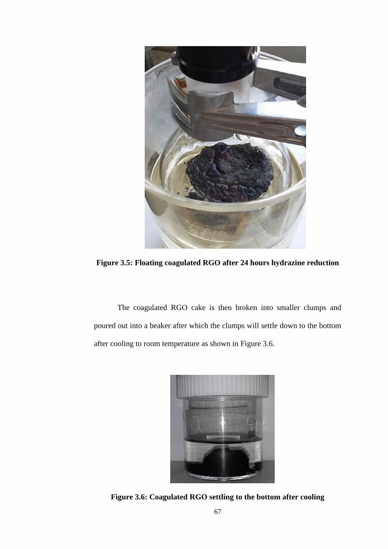
67
Figure 3.5: Floating coagulated RGO after 24 hours hydrazine reduction
The coagulated RGO cake is then broken into smaller clumps and
poured out into a beaker after which the clumps will settle down to the bottom
after cooling to room temperature as shown in Figure 3.6.
Figure 3.6: Coagulated RGO settling to the bottom after cooling

68
The broken RGO clumps are drained out by filter paper then washed
with 100 ml of distilled water followed by 100 ml of ethanol for 5 cycles.
Some of the washed products are kept in ethanol as wet solids and some are
oven dried at 45 ºC for 24 hours and yielded coarse hard particles some larger
than 1 mm as shown in Figure 3.7. This is a poor outcome in the sense that the
surface area to volume ratio of dried RGO is extremely low.
Figure 3.7: Oven dried RGO particles
When the oven dried RGO particles are mixed into DGEBA and hand
stirred vigorously for 30 minutes, they break into smaller sizes but still
remained coarse as shown in Figure 3.8.

69
Figure 3.8: 3% weight oven dried RGO /DGEBA mixture hand stirred
for 30 minutes
In order to overcome this problem, wet and spongy RGO clumps were
press-dried in filter paper to a thickness of 1 mm resulting in a still soft and
slightly moist product. The RGO clumps disintegrated easily into much
smaller particles and were homogenously dispersed after 30 minutes of hand
stirring as shown in Figure 3.9.
Figure 3.9: 3% weight press-dried RGO/DGEBA mixture hand stirred
for 30 minutes

70
The mass of RGO had to be accurately determined due to the presence
of residual ethanol in the press-dried material. Oven drying correlation
experiments were conducted and the weight of press-dried RGO was found to
be eight times (8x) heavier than oven dried RGO. Thus the quantity of press-
dried RGO must be increased by 8x during weighing to obtain the same mass
of dried RGO and thereafter immediately stirred into the DGEBA epoxy while
the filler is still slightly moist and soft.
Even though the residual ethanol should evaporate during the hand
stirring process, each sample must still be allowed to sit at least 30 minutes
prior to further experimental procedures for any remaining ethanol to fully
evaporate. Samples were then prepared and examined using various analytical
techniques as described in the following paragraphs.
Dried samples were examined using the Thermo Scientific Nicolet iS
10 attenuated total reflectance (ATR) FTIR spectrometer to obtain FTIR
spectroscopy data over a wave number range of 4000 – 400 cm-1
at a
resolution of 4 cm-1
. This range corresponds to a wavelength of 2500 nm to 25
µm which is sufficient to study the infrared active oxygen functionalized
groups, i.e. the carboxylic acid (COOH), epoxide (C-O-C), hydroxyl (OH),
and carbonyl(C=O) groups which are supposed to be present in GO as
discussed in chapter 2.

71
An X-ray diffractometer was employed to examine the starter graphite,
GrO and RGO samples. XRD spectroscopy is a technique used to characterize
the crystalline structure of material through the detection and analysis of the
constructive and destructive interference patterns from diffracted incident x-
ray beams. According to Bragg‘s Law the path of diffracted x-ray waves must
obey the following relationship called the Bragg equation (Cullity, 1956):
λ = 2d sin θ (3.1)
where d = crystal interplanar lattice distance (nm)
θ = wave incident angle (degree)
λ = wavelength (nm)
The signal from sample diffraction patterns are collected at an angle of
2θ as illustrated in figure 3.10. The Shimadzu XRD-6000 diffractometer used
to acquire all the experimental diffraction spectra has a monochromatic Cu Kα
radiation source with a wavelength of λ = 1.54 Å (or 0.154 nm). Graphite
(powder), RGO (powder) and GrO (flakes) were loaded on aluminium sample
holders and examined at a 2θ range of 5 degrees up to 70 degrees.

72
Figure 3.10: Schematic of an x-ray beam from a monochromatic source
(T) striking the parallel planes of the crystal sample (C) at an incident
angle θ, then scattering to the detector (D) at a diffraction angle 2θ
(Cullity, 1956)
Raman spectroscopy is an especially useful technique for providing
information on the chemical structures and physical forms of graphene in
terms of lattice disorder, sheet layers, grain boundary, and edge conditions
amongst other characteristics. It can provide a frame of structural reference as
a common denominator for comparing different materials; for example to
distinguish a hard amorphous carbon from a metallic nanotube, graphite from
graphene, or even identify a doped graphene sample by using the Raman shift
spectrum as a fingerprinting technique (Ferrari, 2007).
When light interacts and polarizes the electron cloud surrounding
atomic or molecular nuclei, discrete units of vibrational mechanical energy
called phonons (quasiparticles) are produced. Since this perturbation is an
unstable time-dependent ‗virtual state‘, photons are quickly re-radiated
(scattered) by the short-lived phonons following which the interacting material

73
will stabilize to its original energy state. In elastic (or Rayleigh) scattering, re-
radiated photons are scattered in different directions but retain the same
wavelength as incident photons. However, in the non-resonant inelastic (or
Raman) scattering condition, about one in every 106 to 10
8 re-radiated photon
will have its energy state altered. And if the energy level of the incident
photon happens to be high enough to coincide with the electronic transition
state of the interacting material (resonant condition), it will cause a resonant
effect and this will increase the probability of Raman scattering by several
orders of magnitude. Raman spectroscopy is thus particularly well suited for
analysing graphene since it is a zero band gap material and will always
interact with photons under resonant conditions (Smith and Dent, 2013;
Ferrari and Basko, 2013).
In Raman scattering, a red shift (Stokes scattering) occurs when a re-
radiated photon loses energy while a blue shift (anti-Stokes scattering) occurs
when it gains energy. Figure 3.11 illustrates the Stokes and anti-Stokes
scattering events and their energy states in the resonant condition where
electron-hole pairs are created. The Renishaw in Via confocal Raman
microscope was used to acquire red shifted (Raman shift) signals in Stokes
scattering by filtering out the signals from Rayleigh scatterings. Since anti-
Stokes scattering signals are weak and rare, they are usually ignored. Spectral
bands showing Raman high intensities in many cases have weak infrared
intensities whilst the reverse is also true. Raman spectroscopy and FTIR
absorption spectroscopy are usually performed together to form a pair of
powerful complementary characterization techniques (Smith and Dent, 2013).

74
Figure 3.11: (a) Resonant Stokes scattering: an incoming photon ωL
excites an electron-hole pair e-h. The pair decays into a phonon and
another electron-hole pair e-h′. The latter recombines, emitting a photon
ωSc (b) resonant anti-Stokes scattering: the phonon is absorbed by the
electron-hole pair (c) Energy states of scattering events [Adapted from
Ferrari and Basko, 2013]
XPS also known as Electron Spectroscopy for Chemical Analysis
(ESCA) is a surface-sensitive chemical analysis spectroscopic technique used
for element identification, elemental composition quantification (parts per
thousand range) and the analysis of the chemical state of atoms at the sample
surface down to 10 nm below the surface. In a typical XPS analysis, a
monochromatic soft x-ray beam (typically Al K radiation, hv = 1486.6 eV) is
projected unto a sample placed in a high vacuum chamber. When core
electrons are ejected in a photoemission event, they escape into the vacuum

75
environment as photoelectrons and are detected and counted by an electron
detector while their kinetic energy levels are measured and processed by an
energy analyser to determine their binding energies (Chastain and King,
1992). A schematic of the photoemission effect is shown in Figure 3.12.
The ULVAC-PI Quantera II Scanning XPS Microprobe was used to
acquire the kinetic energies of the emitted photoelectrons and to compute their
corresponding binding energies which are then used as markers to identify the
elements and chemical bonds that are present while the elemental composition
can be established based on the underlying assumption that the number of
electrons detected is proportional to the number of atoms present.
Figure 3.12: Schematic of the photoemission effect. (Adapted from PIRE-
ECCHI, 2015)
Finally samples of the starter graphite, GO and RGO were examined
with the Hitachi S-34000N scanning electron microscope (SEM) equipped
with EDX spectrometer, JEOL JSM-6701F field effect scanning electron

76
microscope (FESEM), and FEI Technai G2 F20 X-Twin high resolution
transmission electron microscope (HRTEM with SAED) for electron imaging
and analysis.
3.4 Rheology Experiments
The Anton Parr Physica MCR 301 rheometer shown in Figure 3.13
was used to perform the rheological experiments. All measurements were
conducted with the 25 mm diameter parallel plate spindle operating at a gap
distance of 0.5 mm. The Peltier plate (bottom non-rotating sample platform)
temperature was set at 25 ºC.
Figure 3.13: Anton Parr MCR301 rheometer (inset: side view of inserted
25 mm parallel plate spindle at a fully raised position)

77
Firstly, DGEBA epoxy resin should be preheated to 50 ºC for at least
30 minutes to ensure that crystallized particles if present are fully melted and
stabilized. This is an important preparatory step to prevent spurious results
caused by recrystallization while rheological measurements are being taken.
RGO filler is then mixed in and hand stirred with a metal spatula at various
concentrations by weight % and subjected to rheological measurements. The
sample mixes and concentrations are shown in Table 3.3.
Table 3.3: Sample formulation and description
Sample name Filler wt. % Filler description
E.P. 0.01% 0.01 Press-dried RGO*
E.P. 0.5% 0.5 Press-dried RGO*
E.P. 1% 1 Press-dried RGO
E.P. 2% 2 Press-dried RGO
E.P. 3% 3 Press-dried RGO
E.P. 4% 4 Press-dried RGO
O.D. 3% 3 Press-dried RGO
Epoxy neat 0 Control sample - pure DGEBA
Graphite 3% 3 Graphite for benchmarking
* Resistivity measurements only
Each sample is then subjected to a constant speed (50 s-1
) flow test to
obtain baseline viscosity measurements, a hysteresis loop test for thixotropy,
yield test for establishing yield stress (if present), and oscillatory amplitude
sweep to define the LVER region followed by a frequency sweep to study the
stability of the dispersion.

78
3.5 Percolation Threshold Measurements
Following the rheological measurements, the samples are hand stirred
vigorously with the curing agent EDA (C2H4(NH2)2), left to harden (pre-cure)
overnight at room temperature and then oven cured at 100 ºC for one hour.
There are four active hydrogen atoms available in the two amine (NH2)
groups for each EDA molecule to provide the bonding reactions with the
epoxide groups of DGEBA molecules. Given that the molar weight (MW) of
EDA is 60.1 g mol-1
and the epoxide equivalent weight (EEW) of the Sigma-
Aldrich DGEBA is 174 g (Sigma-Aldrich, 2015), the stoichiometric ratio in
terms of parts by weight per hundred parts (phr) epoxy resin used for EDA
loading is determined at 8.64 phr by the calculations shown below (DOW
Epoxy, 2015):
phr = amine H eq wt. x 100 / EEW of epoxy (3.2)
= 15.02 / 174
= 8.64
where
amine H eq wt. x 100 =
= 60.01/ 4
= 15.02
It was found that the EDA phr loading of 8.64 phr is sufficient in fully
curing neat epoxy following the curing schedule stated in the first paragraph of

79
this section. But for samples loaded with RGO fillers, the composite remained
soft immediately after oven curing and requires up to several days to fully
harden at room temperature thereafter. The effect of RGO on reducing the
curing efficacy of EDA is not fully understood but this problem is easily
overcome by marginally increasing the amount of EDA added (10% increase
for every 1 g of RGO added) above the stoichiometric ratio. The mold used to
shape and contain the composite samples for curing is a simply four pieces of
pencil erasers carefully squared and glued onto the unplated side of a printed
circuit board as shown in Figure 3.14. Carnauba wax is applied on the exposed
PCB surface as a mold release agent to ensure the easy removal of the cured
samples.
(a) (b)
Figure 3.14: Mold a) Unfilled b) Filled
Once the cured samples are removed they are shaped and hand
polished with sandpaper until the surfaces become flat and the edges squared
as measured with a Vernier caliper. Lastly, any two opposite ends are coated
(smeared) with graphite powder and the samples are now ready for bulk
resistivity measurements as shown in Figure 3.15.

80
Figure 3.15: Finished samples. Graphite coated surface is light grey
The finished samples are securely clamped in a table top vice with the
graphite coated surfaces making firm and even contact with the copper plated
surfaces of two PCB electrodes as shown in Figure 3.16. This is to ensure that
contact surface resistance is reduced to an insignificant level.
Figure 3.16: Setup for resistance measurements
Resistance measurements are made with the Keithley 4200-SCS
parameter analyser which is able to supply forced currents as low as 0.1 x 10-
15 amperes allowing it to measure values up to the 10
12 range. The

81
instrument also has an inbuilt four-point probe feature capable of easily
measuring very low resistances in the µ range. Once the resistance and
physical dimensions of each sample are determined, bulk resistivity (ρ) values
can be computed using equation 2.1 shown in Chapter 2. The various
experimental sample formulations are listed in Table 3.3.

82
CHAPTER 4
4 RESULTS AND DISCUSSION
4.1 GO and RGO Characterization
Since the characterization of GO and RGO requires broadly similar analytical
techniques, the discussion of their test results are therefore organized together
under this section.
4.1.1 Ultraviolet-Visible (UV-Vis) Spectroscopy
The GO oxidized with 4 g of KMnO4 displayed a plasmonic UV
absorption peak at a wavelength of 231 nm coupled with a broad sloping
shoulder around 300 nm due to the n → π* electronic transition in carbonyl
groups. This spectral shape is consistent with that reported by Huang and Lim
et al. (2011). As expected the peak wavelength at 231 nm is slightly longer
than Huang‘s 4.5 g KMnO4 (more oxidized) sample with a peak at 229 nm
because the absorption peaks found at around 230 nm occurred due to the π →
π* electronic orbital transitions from conjugated aromatic C=C bonds; where
the higher the degree of oxidation the fewer remaining conjugated C=C bonds
there are, thus requiring shorter wavelength (more energetic) UV photons to
elicit π → π* electronic transitions.

83
This explanation was verified when a batch of less oxidized GO
prepared using 3 g of KMnO4 showed a plasmon peak at an even longer
wavelength position of 236 nm. For benchmarking purposes, a sample of
Sigma-Aldrich commercial GO was tested and it displayed a spectral pattern
similar to that of the synthesized GO with a peak positioned at 227 nm, refer
to Figure 4.1.
Figure 4.1: UV-Vis absorption spectra
This UV-Vis results taken together with the observation that no
residual graphite flakes were found at the end of the graphite oxidation
process, it is safe to conclude that the GO synthesis process per Huang‘s
method achieved its intended purpose of converting graphite flakes to GO.

84
4.1.2 Fourier Transform Infrared (FTIR) Spectroscopy
Table 4.1 lists the principal infrared absorption bands present in GO and their
corresponding vibrational modes. In comparison, the acquired spectrum for
the synthesized GO sample shown in Figure 4.2 displays the expected
absorption bands present in GO such as O-H stretch at 3700 to 2500 cm–1
,
C=O stretch at 1760 to 1690 cm–1
, and C-O-C stretch at 1250 to 1050 cm–1
.
Table 4.1: Principal infrared absorption bands and corresponding major
vibrational modes for GO functional groups (Adapted from UCLA, 2001;
University of Colorado, 2015) [Accessed on 8 Dec 2015]
Wavenumber (cm–1
) Bond activity Functional group
3640–3610 O–H stretch Hydroxyl
3500–3200 O–H stretch Hydroxyl
3300–2500 O–H stretch Carboxylic acid
1760–1690 C=O stretch Carboxylic acid
1760–1665 C=O stretch Carbonyl
1320–1000 C–O stretch Carboxylic acid
1250–1050 C–O–C stretch Carboxylic acid
1200–1020 C–OH stretch Carboxylic acid
950–910 O–H bend Carboxylic acid

85
Figure 4.2: FTIR spectra for GO, RGO, and Sigma Aldrich GO with
major absorption bands indicated
The unique profile of a spectrum with signature peaks and troughs can
be used as a ‗fingerprint‘ for the identification of a material. The sample
spectrum of Sigma Aldrich GO was acquired for benchmarking purposes. By
visually inspecting the two superimposed curves shown in Figure 4.2, we can
see that they match up relatively well. Differences in the absorption intensities
could be due to variations in the concentration of functional groups as a result
of different oxidising conditions. As for minor differences seen in the
absorption band wavenumbers, Zhang and Dabbs et al. (2015) developed
mathematical models to demonstrate that lattice vacancies could induce both
blue and red shifts in the prominent OH stretching and bending bands.
In contrast, the spectrum for RGO is free from any prominent
absorption troughs and relatively infrared inactive with a transmission level of
60% to 70%. This slightly downward sloping and featureless profile indicate
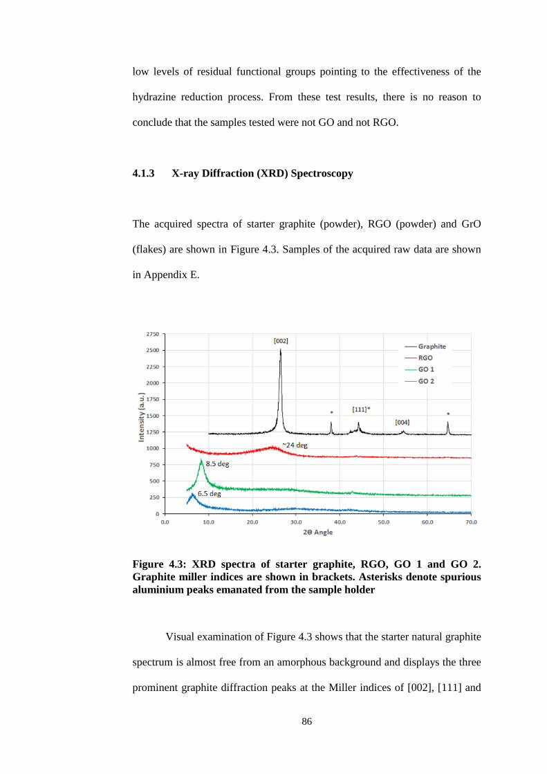
86
low levels of residual functional groups pointing to the effectiveness of the
hydrazine reduction process. From these test results, there is no reason to
conclude that the samples tested were not GO and not RGO.
4.1.3 X-ray Diffraction (XRD) Spectroscopy
The acquired spectra of starter graphite (powder), RGO (powder) and GrO
(flakes) are shown in Figure 4.3. Samples of the acquired raw data are shown
in Appendix E.
Figure 4.3: XRD spectra of starter graphite, RGO, GO 1 and GO 2.
Graphite miller indices are shown in brackets. Asterisks denote spurious
aluminium peaks emanated from the sample holder
Visual examination of Figure 4.3 shows that the starter natural graphite
spectrum is almost free from an amorphous background and displays the three
prominent graphite diffraction peaks at the Miller indices of [002], [111] and

87
[004] providing strong evidence that it is crystalline graphite. Note that the
peaks marked with asterisks are spurious diffractions from the aluminium
specimen holder. At the 44 degree 2θ position there is a slightly broad band
created by the overlapping of the [200] aluminium peak, with the [111]
graphite peak. Table 4.2 lists the diffraction angles, peak intensities, d-spacing
and Miller indices for graphite (RRUFF, 2015a) and aluminium (RRUFF,
2015b) published by the public-private sponsored RRUFF Project created to
collect a worldwide database for mineralogists, geoscientists, and the general
public (Lafuente and Downs et al., 2015).
Table 4.2: Diffraction data for (a) Graphite and (b) Aluminium (Adapted
from RRUFF, 2015a; RRUFF, 2015b)
(a) Graphite:
(b) Aluminium:

88
When the GrO flakes samples were analysed, their spectra showed the
absence of any graphitic diffraction peaks which implies that the starting
material have been completely oxidized. The interplanar distance of graphite
has expanded beyond 0.335 nm due to the intercalation of the d-spacing with
functional groups (Marcano and Kosynkin et al., 2010).
The GrO samples tested were damp, with GO 2 being wetter than GO
1. The presence of the diffused peaks located at 8.5 degrees (d=1.0 nm) for
GO 1 and 6.5 degrees (d=1.3 nm) for the wetter GO 2 are in line with the
expanding effects of moisture (Lerf and Bucksteiner et al., 2006). According
to Stankovich and Dikin et al. (2007), it is very difficult if not impossible to
completely remove moisture from GrO. If the specimen GrO flakes were too
dry it was even necessary to moisten them so that they could be securely
compacted into the shallow indented cavity of the XRD diffractometer sample
holder. Park and Ruoff (2009) postulated that the swelling effects of moisture
caused the interplanar distance to vary from the lowest d-spacing value of d =
0.63 nm for dry GrO to d = 1.2 nm for hydrated GrO. From equation 3.1
(Bragg equation) it can be shown that this d-spacing range corresponds to a 2θ
diffraction angle spanning from 7 degrees (d=1.2 nm) to 14 degrees (d=0.63
nm). This range agrees with the experimental results of Nakajima and Matsuo
(1994) and Lerf and Bucksteiner et al. (2006). Since the peak locations of GO
1 and GO 2 are consistent with this range and are devoid of any graphitic
peaks, it can be concluded that these samples contain fully oxidized GrO.

89
The spectrum of hydrazine reduced RGO sample displays only one
diffused peak near the [002] peak of graphite at 26.4 degrees. This indicates a
partial restoration of graphitic structures into disordered graphene sheets via
the removal of oxygen containing groups (Gao and Ma et al., 2011).
4.1.4 Raman Spectroscopy
The Raman spectra of the starter graphite, GO, and RGO samples are shown
in Figure 4.4 and their corresponding resonant band shifts are tabulated in
Table 4.3.
Figure 4.4: Raman spectra for graphite, RGO, and GO

90
Table 4.3: Raman resonant peaks for graphite, GO, and RGO at 2.41 eV
laser excitation energy (wavelength=514 nm). For comparison, values
published by Jorio (2012) and Ferrari (2007) are shown in the last two
rows
Sample Resonant peaks (cm
-1)
D G 2D (or G’) D+G
Graphite 1,349.4 1,565.4 2,697.7 2,937.7
RGO 1,351.5 1,584.8 2,704.6 2,945.1
GO 1,358.8 1,599.1 2,706.3 2,952.6
Jorio, 2012 1,350.0 1,580.0 2,700.0 2,935.0
Ferrari, 2007 1,360.0 1,560.0 2,710.0 Not stated
An inspection of the RGO and GO spectrum shown in Figure 4.4
reveals several general features consistent with those published by Jorio
(2012) and Ferrari (2007). Prominent and narrow G peaks were detected at ~
1,580 cm-1
band shift, followed by distinct and slightly broader D peaks at ~
1,350 cm-1
band shift while a diffused pair of peaks were detected at the 2D
(or G‘) ~ 2,700 cm-1
and the D + G bands ~ 2,935 cm-1
band shifts.
The G band shifts are produced by single-resonant scattering involving
C-C bond stretching within the in-plane direction. According to various
published literature, the G peak is positioned from 1,560 to 1,582 cm-1
(Ferrari
and Basko, 2013; Jorio, 2012; Ferrari, 2007). In Figure 4.10, RGO has a
higher G peak compared to GO due to the recovery of sp2 domains from the
removal of in-plane functional groups. The position of the G band is not
sensitive to the number of layers as shown in Figure 4.5 (left).

91
Figure 4.5: Evolution of G band (left) and 2D band (right) with respect to
layer thickness (Adapted from Ferrari, 2007)
The D band arises from double-resonant interactions emanating from
edge defects (Jorio, 2012). According to Ferrari and Basko (2013), edges are
regarded as extended defects by breaking the translational symmetry of the
aromatic rings, unless they retain a perfect zigzag or armchair shape which
will then still preserve the symmetry along the edge and thus not contribute to
the D band intensity. This account is useful in explaining the small D peak of
graphite followed by the intense and diffused peak for GO due to the presence
of functional groups breaking up the lattice edges during the oxidation
process. According to Huang and Lim et al., (2011), when GO flakes are
dispersed via ultrasonication prior to the reduction process edge damage will
be introduced due to tearing of the exfoliated sheets. There are also dangling
bonds left behind after the removal of oxygenated functional groups.
According to Stankovich and Dikin et al. (2007) the average size of the
recovered sp2 domains are also smaller compared to their prior dimensions as

92
sp3 sites in the exfoliated GO sheets. Therefore RGO has a more intense D
peak compared to GO because it contains relatively more disordered edges.
The 2D band is an overtone of the D band. For pristine single layered
graphene (SLG), a very intense 2D peak is detected at a Raman shift of
slightly less than 2,700 cm-1
. This feature is used as the fingerprint for
confirming SLG. When the layers increase to two layers and beyond, the 2D
band will evolve from a sharp single peak to broader convoluted peaks as
shown in Figure 4.5 (right). The difference between the spectrum of SLG and
that of graphite can be clearly distinguished by examining their G and 2D
bands as shown in Figure 4.6. Note that the 2D to G peak ratio (I2D / IG) is less
than unity for graphite and greater than unity for SLG. The number of layers
present can be derived from the ratio of the I2D / IG peak intensities, as well as
the position and shape of these peaks as discussed earlier (Childres and
Jauregui et al., 2013).
Figure 4.6: Raman shift of single-layered graphene (top) versus graphite
(Adapted from Ferrari, 2007)

93
The RGO and GO spectra showed in Figure 4.4 display prominent but
slightly broad D and G bands with low intensity diffused 2D and D + G bands.
For RGO, these features can indicate the presence of edge defects and in-plane
disorder and impurities in the crystal lattice. Since the I2D / IG peak ratio is less
than unity, the RGO obtained is multi-layered. Unfortunately, due to the high
level of diffusion present in the 2D peak the number of layers cannot be
resolved. The peak intensities and ratios for the D, G, and 2D bands are
summarized in Table 4.4.
Table 4.4: Peak intensities and intensity ratios
Sample Peak intensity (cps) Intensity ratio
ID IG I2D ID/IG I2D / IG
Graphite 305.85 1,583.65 922.46 0.19 0.58
RGO 8,583.03 7,936.18 1,531.97 1.08 0.19
GO 6,260.47 6,900.84 3,243.24 0.91 0.47
Stankovich and Dikin et al. (2007) obtained similar D and G band
profiles as shown in Figure 4.7. Note that the near zero intensity of the D band
for graphite is explained by the low defect purified natural graphite used.

94
Figure 4.7: Raman spectra showing D and G bands for graphite, GO, and
RGO (Adapted from Stankovich and Dikin et al., 2007)
Based on the preceding discussions on the Raman spectroscopy results,
it can be concluded that the synthesized RGO is consistent with that produced
by the process developed by Stankovich and Dikin et al. in 2007.
4.1.5 X-ray Photoelectron Spectroscopy (XPS)
Figures 4.8 and 4.9 are the broad survey scans for GO and RGO generated by
the XPS energy analyser. The O KLL peaks are Auger electron signals and
therefore can be ignored.

95
Figure 4.8: XPS broad survey scan for GO
Figure 4.9: XPS broad survey scan for RGO
As expected the survey scan for GO shown in Figure 4.8 contains a
sharp and intense oxygen peak at the O1s position with the presence of a
relatively small carbon C1s peak. There are also prominent phosphorous and

96
sulphur peaks present. But unexpectedly, the C/O ratio of 0.30 is much lower
than the 2.7:1 ratio reported by Stankovich and Dikin et al. (2007). This
lowered ratio is very likely due to the oxygen contained in the residual
phosphate and sulphate salts probably as a result of the inadequate wash
process.
As for the RGO broad survey scan shown in Figure 4.9, the C/O ratio
of 6.8 indicates a significant removal of oxygen bearing functional groups via
the hydrazine reduction process. This observation is corroborated by the FTIR
results discussed earlier in section 4.1.2. In comparison, Dreyer and Park et al.
(2010) reported a C/O ratio in the range of 2.8 to 6.2 for RGO films, while
Marcano and Kosynkin et al. (2010) reported a C/O ratio of around 10:1 for
RGO that have been thermally annealed. Note that phosphorous peaks are no
longer present while sulphur peaks have been reduced to near zero levels most
likely because the sulphate and phosphate salts were removed during the RGO
wash process. The detection of minor silicon peaks could be due to
contamination from the glassware used.
The presence of a significant nitrogen N1s peak at a C:N ratio of
18.4:1 is caused by doped nitrogen atoms from the hydrazine used. During the
reduction process, nitrogen atoms tend to form covalent bonds at the surface
of GO sheets while the oxygen bearing groups are being removed resulting in
amines, hydrazones, aziridines and other similar structures. Functioning as an
n-type dopant, such heteroatomic impurities have a profound disrupting effect

97
on the sp2 structure of the final RGO lattice. According to Dreyer and Park
(2010), the C to N doping ratio can go as low as 16:1.
The deconvoluted narrow scans at C1s for GO and RGO with the
appended binding energies of the various bonds are shown in Figures 4.10 and
4.11 respectively. C-C denotes carbon to carbon sp2 bond, C-O denotes single
hydroxyl bond and epoxide functionality, C=O denotes carbonyl bond, C(O)O
denotes carboxylic bond, and pi – pi* transition denotes the bond to anti-
bond transition. The binding energies were produced by the PHI-Quantera
XPS spectrum analyser software. These values are consistent with those
published by Park and An et al. (2011), Marcano and Kosynkin et al. (2010),
and Stankovich and Dikin et al. (2007).
Figure 4.10: XPS deconvoluted C1s spectrum for GO

98
Figure 4.11: XPS deconvoluted C1s spectrum for RGO
The highly oxygenated GO spectrum and the largely deoxygenated
RGO spectrum are consistent with the curves published by Park and An
(2011) shown in Figure 4.12. In terms of C-O/C-C bond evolution, the purity
of RGO from figure 4.11 is calculated at a C-O/C-C ratio of 0.16 in contrast
with its precursor state calculated at a ratio of 1.21 as shown in figure 4.10.
Figure 4.12: XPS C1s spectra for GO and RGO (Adapted from Park and
An, 2011)

99
In summary, the XPS elemental analysis results point to a highly
oxidized GO which contained some residual sulphate and phosphate salts that
were eventually removed during the RGO reduction process. The synthesized
RGO was well deoxygenated consistent with the ranges published in highly
cited research articles and contained doped nitrogen due to the hydrazine
(reducing agent) used.
4.1.6 Electron Microscopy
The FESEM image of the Asbury Carbon Nano 25 grade graphite flakes used
as starter material for the synthesis of GO is presented in figure 4.13.
Figure 4.13: Asbury Carbon Nano 25 grade natural graphite flakes

100
This grade of graphite was selected because it was processed from
natural graphite into thin flakes of several microns to tens of microns in
dimension to specifically facilitate the intercalation of the graphite d-spacing
with oxygenated functional groups. The presence of pristine graphitic
hexagonal crystal lattice can be clearly seen. However some rounded edges on
the stacked features indicate edge damage probably sustained during
production. Note that the presence of impurities (see bottom left hand and top
right hand corners) is likely to be amorphous carbon residue because an EDX
analysis showed that the material contained only carbon (97%) and oxygen
(3%).

101
Figure 4.14 is the FESEM images of dried GO flakes showing
prominent surface folds at different magnifications.
Figure 4.14: FESEM images of dried GO flake. Compacted thick folds
feature prominently at X10k magnification (top) and X33k (bottom)
magnified close-up view

102
Figure 4.15 displays the FESEM images of dried RGO particles
showing stacked agglomerates with corrugated wrinkled surface morphology.
Figure 4.15: FESEM images of dried RGO particles. Edge view shows
stacked agglomerated sheets of graphene (top) and X45k magnified
surface view showing the wrinkling effect of single or few layered
graphene

103
Figure 4.16: HRTEM images at X6.3k magnification for GO (top) and
HRGO (bottom) sheets suspended on lacey carbon TEM grid. Dried GrO
flakes and RGO particles were ultrasonicated for 30 minutes in ethanol,
drop casted and air dried
HRTEM high resolution images were obtained for exfoliated GrO and
RGO sheets to study their surface and edge morphology. Visual inspection of

104
low magnification HRTEM images for exfoliated GrO and RGO sheets shown
in Figure 4.16 reveal a distinct difference between the two materials. Being
thicker due to the presence of functional groups attached to the basal plane, the
GO sheet(s) appear relatively flat and less crumpled compared to the RGO
sheet(s) which is wrinkled and contains many folded and crumpled zones. At a
higher magnification, the characteristic wrinkling and corrugated features of
the suspended RGO sheet are clearly visible as shown in Figure 4.17. Note
that the curling or scrolling at the unsupported hanging edges visible at the
bottom of the figure is a common feature of single and few layered graphene
sheets according to Meyer and Geim et al. (2007)
Figure 4.17: RGO at X17.5k magnification revealing the wrinkling, folded
and heavily crumpled features with scrolled edges (bottom of image) of
freely suspended single and/or few layered graphene sheets
At higher magnifications, the number of layers in a graphene sheet will
only be visible if wrinkled or folded sheets are imaged at an angle

105
perpendicular to the fold. This is not difficult to accomplish because folded
regions are abundantly present in the sample. Figure 4.18 shows an image at
X255k magnification with a 5-layered sheet thickness.
Figure 4.18: Folded region of few layered RGO sheet at X255k
magnification. A wrinkled feature (inside red oval) viewed from one side
revealing a 5-layered sheet thickness at ~ 0.335 nm sheet distance

106
An explanation of how the number of layers can be resolved via
HRTEM imaging is illustrated in Figure 4.19 by Meyer and Geim et al.
(2007).
Figure 4.19: How folded (including wrinkled and creased) sheet edges
show up in a TEM image according to Meyer. Scale bars = 2nm (Adapted
from Meyer and Geim et al., 2007)
With selected area electron diffraction (SAED) spectroscopy, a
selected area of the HRTEM image can be tested to determine if the sample is
crystalline, polycrystalline, or amorphous. Figure 4.20 is an image of RGO
obtained at 800k magnification showing an amorphous basal plane.

107
Figure 4.20: RGO at X800k magnification showing disordered basal
lattice structure and an irregular edge. SAED diffraction pattern (inset)
indicates a highly amorphous structure. Faintly visible graphitic
hexagonal diffraction spots are pointed out with red arrows
The lack of crystalline structure in the SAED diffraction pattern was
most likely caused by the destructive power of the high energy electron beam
set at 200keV while the image was being acquired. According to Kotakoski
and Meyer (2011), point defects especially vacancies are naturally created by
the ―knock-on‖ effect from energetic electrons if the threshold beam energy of
100 keV is exceeded. This effect is more acute at higher magnifications and at
longer dwell times. The skill of the HRTEM imaging operator is thus very
important in determining the quality of the images obtained. Fortunately, the
young operator at MIMOS subsequently improved his technique and managed
to obtain better quality GO and RGO images. Figure 4.21 (used with
permission) is an image of RGO produced by Tan (2015) in her Final Year
Project work at UTAR using Marcano‘s process showing a clear graphitic

108
crystalline lattice structure even though the lattice sustained some damage
during image acquisition.
Figure 4.21: RGO (Marcano’s process) at X930k magnification (Adapted
from Tan (2015) with permission)
Damage caused by the HRTEM imaging process notwithstanding, it
was also pointed out in section 2.3.3 of the literature review that the wet
reduction of GO to RGO is a process which produces inherent edge and basal
plane lattice defects. An RGO image populated with basal plane vacancies not
exceeding 100 nm across is shown in Figure 4.22. Any damage caused by the
electron beam is minimal because the image was acquired at a relatively low
26.5k magnification where the destructive effects of the beam are spread out
over a wider area.

109
Figure 4.22: RGO at X26.5k magnification. Basal plane with vacancy type
lattice defects visible at bottom left region of image
In summary, the FESEM and HRTEM image analysis showed that GO
and RGO can be identified and differentiated. The synthesized RGO sheets
were few layers thick and their surface and edge morphology contained
defects such as vacancies and disordered non-crystalline lattice structures.
Supplementary images are shown in Appendix B.
4.2 Rheological Characterization
The rheological properties of the RGO filled epoxy samples were studied per
the formulations listed in Table 3.1. The 25 mm diameter parallel plate gap
distance was fixed at 0.5 mm and temperature controlled at 25 ºC. Following
are the results and discussions for the flow and oscillatory rheological test

110
measurements made. Samples of rheometer raw data are shown in Appendix
C.
4.2.1 Constant Shear Test
The constant shear test is a flow study that will give an indication of fluid
stability under shear over time. The stencil or screen printing process typically
used for the application of the liquid ICA operates over a period of seconds at
the shear rate of around 10 to 102 s
-1 (Barnes, 2000). Therefore a shear rate ( )
of 50 s-1
was selected to obtain viscosity measurements and provide a
fundamental understanding of the matrix under this constant flow condition.
All the curves in Figure 4.29 are flat. This means that the samples do
not shear thin thus displaying a stable Newtonian like behaviour within the
experimental time interval of 120 s. The measured viscosity of 4.38 Pa.s for
neat epoxy is within the range specified by the manufacturer (Sigma-Aldrich,
2015). The measurements for the oven-dried RGO samples were omitted
because the data points obtained were highly erratic due to the coarse particles
breaking up in the matrix while the samples were being measured. Because of
this, the oven-dried samples were left out of all subsequent experiments.

111
Figure 4.23: Viscosity measurements at constant shear rate ( 50 s-1
The viscosity of the samples increased non-linearly with the increase in
filler loading starting at a viscosity of 7.3 Pa.s at 1% filler loading reaching a
value of 50 Pa.s for the E.P. 4% sample. Viscosity is the resistance of a fluid
to flow. The presence of the agglomerated irregularly shaped granular RGO
particles provides this resistance by impeding the flow of the DGEBA
molecules past each other. Interestingly, the viscosity of the 3% graphite filled
benchmark sample at 4.39 Pa.s was not significantly larger than that of the
neat epoxy. This can be explained by the low resistance smooth laminar flow
between the shear planes due to the lubricating effect of the uniformly aligned
graphitic micro sheets. But as the concentration of the non-uniform granular
RGO particles increased, the flow of the DGEBA molecules probably became
even more turbulent thus increasing the viscosity significantly along the way.

112
4.2.2 Hysteresis Loop Test
It was pointed out in the literature review section that Newtonian fluids will
display non-Newtonian like behaviour when subjected to high enough shear
rates. The hysteresis loop test is a flow test that can reveal the shear thinning
(or thickening) profile together with any time-dependent property (thixotropic
characteristic) of a fluid.
Figure 4.30 illustrates the curves of the hysteresis loop tests conducted
on the experimental samples where the shear rate was increased from zero to
600 s-1
over a 160 s duration and reversed along the same path back to zero
following a 15 s constant shear interval at 600 s-1
. The graphite 3% sample
curve is omitted because it overlaps with the epoxy neat curve.
Figure 4.24: Hysteresis loop curves

113
The unfilled epoxy sample does no exhibit a clear hysteresis loop
(refer to Figure 2.22 for a typical example) since the forward and return stress
curves overlap each other. The near linear shape also points to minimal shear
thinning. This result supports the earlier conclusion from the constant shear
test that pure epoxy is an unstructured Newtonian like fluid.
When epoxy is filled with 1% RGO, a very narrow hysteresis loop
appeared. This shear thinning effect is most likely caused by the breakdown of
the matrix micro structure created by the presence of RGO particles in the
matrix. A schematic of this phenomenon is illustrated in Figure 2.17 where
completely unstructured or minimally structured fluids exhibit shear thinning
behaviour. As the content of the filler increases the hysteresis loop became
more prominent with the 4% filled sample showing the largest loop with a
distinct time dependent drop in shear stress before the return curve. This
presence of a looping feature accompanied with a drop in shear stress during
the constant shear interval is a characteristic of thixotropic materials (Barnes,
2000).
The relative overall increase in shear stresses corresponding to the
filler content supports the finding of the constant shear test that viscosity
increased along with filler concentrations. The fact that the return shear stress
curve of every sample ended at their points of origin indicate that the matrix
managed to recover to their initial rest structures. This is noteworthy because
the RGO filled epoxy composites did not suffer any permanent breakdown and
thus are very stable within these shear conditions.

114
4.2.3 Amplitude Sweep Test
Figure 4.31 illustrates the amplitude sweep curves conducted at a fixed
angular frequency (ω) of 10 s-1
over a strain (γ) range of 0.01 to 100 (%). The
distinct linear viscoelastic regions (LVERs) of the 2% to 4% RGO filled
samples extended up to the 1% limiting strain level beyond which non-linear
behaviour started to gradually emerge. From around 10% strain onwards the
samples transitioned into the non-linear viscoelastic region. Hence the
midpoint of 5% strain was selected as the parameter for the frequency sweep
test since the amplitude sweep test is an oscillatory test designed to elucidate
the viscous and elastic (if present) behaviour of a sample by measuring the G‘
(storage modulus) and G‖ (loss modulus) values when subjected to an
increasing oscillatory shear strain at a fixed strain rate.
With the exception of the 4% RGO filled sample, the rest of the
samples displayed liquid-like behaviour because their loss moduli G‖ were
always above their storage moduli G‘ and also did not display any cross-over
points throughout the full range of the experiments. The 4% filled RGO
displayed a different characteristic from the rest of the samples at which its
storage modulus G‘ dominated the loss modulus G‖. This indicates that
beyond 3% filler loading, there exists a threshold at which the RGO matrix
transitioned from liquid-like to solid-like behaviour from a rheological
perspective. This observation corresponds well with the difficulty encountered
during the hand mixing of the sample when the dispersion of the particles took
longer than usual due to its thick and tacky consistency.

115
Figure 4.25: Amplitude sweep curves at ω = 10 s-1
As for the epoxy neat, E.P. 1%, and the graphite 3% samples their low
and unstable G‘ curves accompanied with prominent G‖ curves yielding large
loss tangent (δ) values (δ = G‖/G‘ refer to equation 2.11) in the range of 10 to
104. A loss tangent value of greater than one indicates that the material is
viscous in nature and the larger the δ value the more dominant the viscous
behaviour is. In the case of unfilled epoxy at the point where G‖/G‘ is
46/0.018, the loss tangent is a massive 2,556 pointing to a viscous fluid with a
virtually non-existent Hookean elasticity characteristic. This result
corroborates the findings from the constant shear and hysteresis loop tests.

116
4.2.4 Frequency Sweep Test
Following the amplitude sweep test, the amplitude of the frequency tests were
fixed at 5% strain (γ) and the experimental results are shown in Figure 4.32.
The frequency sweep is an oscillatory test at which the amplitude of
oscillation (a value around the LVER identified from the amplitude sweep test
where the internal structure is expected to remain stable) is held constant while
the angular frequency of oscillation (ω) is typically varied over a range of 10-1
to 102 s
-1 (Willenbacher and Georgieva, 2013; Barnes, 2000).
The shape and the magnitude of the frequency sweep curves depend
largely on the internal structure of the material. The behaviour of the samples
started at the rubbery/plateau region then moved into the leathery/transition
zone within the experimental frequency sweep range with the 4% RGO filled
epoxy demonstrating the second G‘/G‖ crossover point at ω = 10 s-1
to demark
the onset of the transition between the two zones (refer to Figure 2.25. for an
illustration of the general shape of viscoelastic behaviour). The almost
overlapping G‘ and G‖ moduli of the neat epoxy up to the 3% RGO filled
samples indicate that little internal structure exists at those concentrations. As
detected at the constant shear, hysteresis loop, and amplitude sweep tests, the
4% filler concentration level imparted a structural behaviour to the epoxy
matrix not apparent in the other samples.

117
Figure 4.26: Frequency sweep at γ = 5%
As the angular frequency is increased, the short-term time-dependent
behaviour of the material dominates leading to an increase in rigidity in the
matrix. The downward sloping complex viscosity curves of all the samples can
be explained in terms of the loss tangent increasing with frequency even
though the storage modulus G‘ increased along the way albeit at a slower rate
(this can be more clearly seen by examining the 4% RGO curves). As the
frequency is increased, the heat dissipated within the matrix is transferred out
through the cooling effect of the rheometer Peltier plate in keeping the
working temperature constant at 25 ºC.
Even though the experiments conducted were limited to a typical
range, a series of time-temperature superposition (TTS) curves can be

118
obtained at different temperatures at the same oscillation rates to construct
what is known as a master curve in order to extend the range of the frequency
sweep curves if so required (Barnes, 2000).
4.2.5 Yield Test
Since the yield test is a flow experiment used to investigate how a fluid
deforms at rest and transitions to flow (yield-to-flow) when subjected to a
controlled increased in shear rate, it can be seen from Figure 4.33 that as shear
rate was increased the shear stresses also increased immediately from the point
of origin in a linear pattern for the neat epoxy and 1% RGO filled samples.
Together with their almost flat viscosity curves it is clear that these two
specimens do not exhibit significant yield-to-flow characteristics. Inspection
of the other shear stress curves show that yield-to-flow behaviour began to
emerge only at the 2% RGO concentration onwards with the 4% RGO filled
sample showing the highest yield stress of 580 Pa.
The concentration of the filler affects the micro-mechanical structural
property of the samples and plays a large role in the yield-to-flow behaviour of
the matrix. The 2% filler level appears to be the threshold upon which the
resistance offered by the higher particle concentration required a yield stress to
be built up first before structural breakdown allowed the matrix to flow. This
general behaviour of the RGO filled composite matrix correlates well with that
shown in Figure 2.20 of the literature review.

119
Figure 4.27: Yield test curves
4.2.6 Summary of Rheological Characterization
Neat DGEBA epoxy resin is a robust Newtonian-like fluid which did not
undergo permanent changes in its polymeric micro-structure even at shear
rates of up to 600 s-1
. With these characteristics, it is well suited as a
composite binder material for ECAs.
RGO filled epoxy matrix is a thixotropic and viscoelastic composite.
The behaviour of the matrix transformed gradually as filler concentration was
increased. But at the 4% concentration level, it exhibited a large shift in
rheological behaviour and transformed into a tacky thixotropic viscoelastic
material. This highly structured gel like behaviour as seen in the
predominantly linear and upward sloping G‘ modulus in the frequency sweep

120
test points to a stable formulation that would not result in particulate
sedimentation over time.
4.3 Bulk Resistivity Measurements
From the curve of the bulk resistivity measurements shown in Figure 4.34,
RGO filled DGEBA epoxy matrix has a percolation threshold of Pc = 0.7%.
Extrapolation of the curve shows that the bulk resistivity should plateau out at
around 1.00E+01 cm. These characteristics are similar to the findings of
Stankovich and Dikin el al (2007) as shown in Figure 2.28. Sample
calculations for bulk resistivity and the measured corresponding resistance
values are shown in Appendix A.
As shown in the results obtained by Park and An (2011) in figure 4.12,
the purity of RGO defined by the C-O/C-C ratio can go as low as near zero. If
the purity of the synthesized RGO at a C-O/C-C ratio of 0.16 is lowered, a
concomitant improvement in the electrical conductivity of the ‗cleaner‘ RGO
loaded ICA can be surmised. However, due to a lack of data points in this
research effort, only a further study can quantify the relationship of C-O
impurity with respect to the bulk resistivity of RGO filled ICA.

121
Figure 4.28: Bulk resistivity (ρ) measurements
For benchmarking purposes, both the 3% filled graphite and oven dried
RGO samples were found to be less conductive by three orders of magnitude
compared to the same amount of ethanol pressed RGO. As discussed in the
literature review chapter, evenly dispersed small particles of RGO particles are
the major factors in influencing the conductivity of ICAs. A picture of the
fractured surface of a 1% ethanol pressed RGO cured sample examined under
an optical microscope is shown in Figure 4.29 displaying a somewhat even
level of particle dispersion but with a wide distribution of particle sizes in the
range of a few microns to tens of microns in dimension.

122
Figure 4.29: Optical micrograph of the fractured surface of a cured
sample matrix filled with 1% ethanol pressed RGO. Particles are black
and the light coloured background is the surface of the epoxy binder
Figure 4.30 is the FESEM images of the same sample. Even though the
contrast of the RGO filler and epoxy binder is poorer compared to the optical
image, the image produced from a 90º viewing angle and at a higher resolution
gives a clearer understanding of how the RGO particles are dispersed and the
morphology of the microstructural network in forming the conductive
pathways of the ICA. At higher filler loadings, the images obtained were not
informative because the higher density of particles obscured the background
and therefore did not show up as distinct entities.

123
Figure 4.30: FESEM micrographs of the fractured surface of a cured
sample matrix filled with 1% ethanol pressed RGO (top), and at higher
magnification (bottom)

124
It can be clearly seen that the islands of agglomerated particles are
separated by gaps with bridging points occurring randomly. Since the 1% filler
concentration is above the percolation threshold of 0.7%, the number of
bridging points must be sufficient enough in forming a closed circuit network
across the bulk of the sample. Voids present in the samples are probably
caused by the outgassing of unreacted curing agent during the curing process
and may have a detrimental reliability impact in terms of mechanical moduli
reduction and moisture absorption into the matrix. Possible solutions for
reducing the number voids is to mix an amount of curing agent at slightly
below stoichiometric ratio or by subjecting the mixture to horn ultrasonication.
In summary, two primary groups of factors affect the bulk resistivity of
the RGO filled ICA – purity/lattice structure of the synthesized RGO and the
size/dispersion of the RGO particles in the binder material. Further studies
have to be conducted to develop a deeper understanding on how these factors
affect bulk resistivity and to quantify their interactions (if any) in lowering the
bulk resistivity of RGO filled ICAs.

125
CHAPTER 5
5 CONCLUSION AND RECOMMENDATION
5.1 Graphene Synthesis
The synthesis of graphene via the Huang and Lim et al. (2011) aqueous
process of oxidizing natural graphite flakes into GO followed by chemical
reducing using the Stankovich and Dikin et al. (2007) technique to RGO is a
viable technique for producing graphene. Due to the hydrophobic nature of
graphene the synthesized RGO took on the morphology of agglomerated
particles consisting stacked graphene sheets when samples were examined
with the FESEM. When viewed under the HRTEM at X255k magnification,
one of the folded regions of an exfoliated RGO particle revealed a 5-layered
sheet thickness measured at ~ 0.335 nm inter-sheet gaps.
Further HRTEM micrograph analyses provided clear visual evidence
which revealed significant in-plane and edge topographical defects while the
presence of distinct Raman peaks at the band shifts of D ~ 1,351.5 cm-1
, G ~
1,584.8 cm-1
, 2D (or G‘) ~ 2,704.6 cm-1
, D + G ~ 2,945.1 cm-1
and their peak
intensity ratios of ID/IG = 1.08 and I2D / IG = 0.19 support the conclusion that
the synthesized RGO is indeed graphene. Together with the deconvoluted XPS
C1s spectrum showing a highly significant C-N peak at 285.8 eV, it can be
concluded that the synthesized RGO is topographically imperfect graphene

126
containing heteroatomic contaminations mainly as doped nitrogen atoms at a
C-O/C-C purity ratio of 0.16.
5.2 Rheology Studies of RGO Dispersion in DGEBA
Flow and oscillatory rheological tests showed that RGO filled epoxy
composite is predominantly Newtonian like in behaviour at a weight
concentration of 1% gradually transitioning to non-Newtonian behaviour with
shear thinning and thixotropic characteristics as filler content increased to 3%
loading. At the 4% weight concentration level, a step change in characteristic
occurred when the matrix displayed a more structured gel like behaviour.
It can be concluded that semi-wet RGO particles can be evenly
dispersed in DGEBA epoxy forming a highly robust and stable liquid matrix
which is a desirable characteristic in the electronics industry where syringe
dispensing and screen printing processes are used. In reference to the findings
published by Santamaria and Munoz et al. (2013), Lu and Tong et al. (1999),
Dreyer and Ruoff et al. (2010) and Morris (2007) this new observation of
semi-wet RGO filled matrix behaviour in ICA research has useful implications
extending beyond the field of electronics packaging and interconnects to other
areas such as lubrication technologies and paint and coating applications.

127
5.3 ICA Electrical Percolation Threshold
Bulk resistivity measurements showed that DGEBA epoxy filled with
synthesized RGO displayed a percolation threshold of Pc = 0.7% loading by
weight at a bulk resistivity of 1.50E+05 cm. The conductivity behaviour of
epoxy loaded with RGO from 1% to 4% by weight is consistent with that of an
ICA. However, with the minimum bulk resistivity extrapolated at not lower
than 1.00E+01 cm this value is still six orders in magnitude higher than that
of Sn/Pb solder at 1.50E-05 cm. Based on this finding, the synthesized RGO
filled epoxy matrix is not conductive enough to be used as a replacement for
Sn/Pb type solder.
Optical and FESEM images of fractured samples managed to reveal
the morphology of RGO filler material trapped within the epoxy binder
material. Conductive pathways are formed through a network of dispersed
RGO particles making physical contact with each other. This point to the
relatively large size of agglomerated particles and the poor quality of the
synthesized RGO as the limiting factors in attaining better electrical
conductivity.
5.4 Recommendations
GO is hydrophilic and therefore disperses well in water. RGO on the other
hand is hydrophobic and the particles begin to aggregate and agglomerate
immediately upon reduction due to their high surface energies. In theory, the

128
conductivity of RGO filled ICA should increase if the filler particles can be
stabilized at the dimension of just a few layers or even down to single sheets.
Since it is possible in theory to keep the nano-dimensioned RGO sheets apart
through the use of dispersing agents, particle dispersion experiments via the
application of stearic and non-stearic surfactants might be useful.
The application of graphene nano-coatings via the in situ reduction of
GO coatings is another area of research worth pursuing. Since GO is water
soluble, a thin coating can readily be applied on specimen surfaces and
subsequently reduced to an RGO layer by exposing the coated material to
hydrazine vapour.
Given that the ACS Material graphene powder purchased from the
United States that was used in initial experiments turned out to be not
conductive and from SEM analysis appeared very likely to be exfoliated and
partially reduced GO, the lesson learnt here is not to accept at face value the
manufacturer‘s certification and to always verify the quality of commercially
available graphene before use. From an equipment perspective, the addition of
a horn ultrasonicator and a zeta potential analyser would be useful
enhancements for our laboratory in conducting future nano-materials
experiments.

129
5 REFERENCES
Areshkin, D.A., Gunlycke, D. and White, C.T., 2007. Ballistic transport in
graphene nanostrips in the presence of disorder: Importance of edge effects.
Nano Letters, 7(1), pp.204-210.
Bae, S., Kim, H., Lee, Y., Xu, X., Park, J.S., Zheng, Y., Balakrishnan, J., Lei,
T., Kim, H.R., Song, Y.I. and Kim, Y.J., 2010. Roll-to-roll production of 30-
inch graphene films for transparent electrodes. Nature nanotechnology, 5(8),
pp.574-578.
Bagri, A., Mattevi, C., Acik, M., Chabal, Y.J., Chhowalla, M. and Shenoy,
V.B., 2010. Structural evolution during the reduction of chemically derived
graphene oxide. Nature chemistry, 2(7), pp.581-587.
Barnes, H.A., 1997. Thixotropy—a review. Journal of Non-Newtonian fluid
mechanics, 70(1), pp.1-33.
Barnes, H.A., 1999. The yield stress—a review or ‗πανηα ρει‘—everything
flows?. Journal of Non-Newtonian Fluid Mechanics, 81(1), pp.133-178.
Barnes, H.A., 2000. A handbook of elementary rheology. Institute of non-
Newtonian Fluid Mechanics, University of Wales. Aberystwyth.
Barnes, H.A., Hutton, J.F. and Walters, K., 1989. An introduction to rheology
(Vol. 3). Elsevier.
Bellinger, D.C. and Bellinger, A.M., 2006. Childhood lead poisoning: the
torturous path from science to policy. Journal of Clinical Investigation,
116(4), p.853.
Biró, L. P., P. Nemes-Incze, et al., 2012. Graphene: nanoscale processing and
recent applications. Nanoscale, 4(6), pp.1824-1839.

130
Bonaccorso, F., Lombardo, A., Hasan, T., Sun, Z., Colombo, L. and Ferrari,
A.C., 2012. Production and processing of graphene and 2d crystals. Materials
Today, 15(12), pp.564-589.
Brodie, B.C., 1859. On the atomic weight of graphite. Philosophical
Transactions of the Royal Society of London, pp.249-259.
Chastain, J. and King, R.C. eds., 1992. Handbook of X-ray photoelectron
spectroscopy: a reference book of standard spectra for identification and
interpretation of XPS data (p. 261). Eden Prairie, MN: Perkin-Elmer.
Childres, I., Jauregui, L.A., Park, W., Cao, H. and Chen, Y.P., 2013. Raman
spectroscopy of graphene and related materials. New developments in photon
and materials research, 1, pp.978-981.
Creative Commons, 2015. A piece of resistive material with electrical
contacts on both ends. [Online] Wikipedia. Available at:
<https://commons.wikimedia.org/wiki/File:Resistivity_geometry.png>
[Accessed 19 November 2015]
Cullity, B.D., 1956. Elements of X-ray Diffraction. Adisson-Wesley
Publishing. USA.
Dow Answer Center, 2015. Dow-epoxy-calculation-of-stoichiometric-ratios.
[Online] Midland: Dow Corning Corporation. Available at:
<http://dowac.custhelp.com/app/answers/detail/a_id/4151/~/dow-epoxy---
calculation-of-stoichiometric-ratios> [Accessed 2 December 2015].
Dow Corning, 2015. IMAGINE: Reliable adhesion in extreme conditions.
[Online] Midland: Dow Corning Corporation. Available at:
<https://www.dowcorning.com/content/electronics/electronicsproducts/sapm-
die-attach-adhesives.aspx> [Accessed 10 December 2015].
Dreyer, D.R., Park, S., Bielawski, C.W. and Ruoff, R.S., 2010. The chemistry
of graphene oxide. Chemical Society Reviews, 39(1), pp.228-240.

131
Dreyer, D.R., Ruoff, R.S. and Bielawski, C.W., 2010. From conception to
realization: an historial account of graphene and some perspectives for its
future. Angewandte Chemie International Edition, 49(49), pp.9336-9344.
Du, J. and Cheng, H.M., 2012. The fabrication, properties, and uses of
graphene/polymer composites. Macromolecular Chemistry and Physics,
213(10‐11), pp.1060-1077.
Duffy, J.J., Hill, A., Walton, A. and Mazzeo, F., 2011. Suspension stability;
Why particle size, zeta potential and rheology are important. Proceedings of
Particulate Systems Analysis.
Environment Directorate General of the European Commission, 2009. Waste
Electrical and Electronic Equipment (WEEE). [Online] Brussels: European
Commission. Available at: <http://ec. europa.
eu/environment/waste/weee/index_en. htm> [Accessed 10 December 2015].
EPOTEK, 2015. EPO-TEK E3001 Technical Data Sheet. [Online] Pembroke
Pines:, Epoxy Technology, Inc. Available at: <
http://www.epotek.com/site/administrator/components/com_products/assets/fil
es/Style_Uploads/E3001.pdf> [Accessed 10 December 2015].
Ferrari, A.C., 2007. Raman spectroscopy of graphene and graphite: disorder,
electron–phonon coupling, doping and nonadiabatic effects. Solid state
communications, 143(1), pp.47-57.
Ferrari, A.C. and Basko, D.M., 2013. Raman spectroscopy as a versatile tool
for studying the properties of graphene. Nature nanotechnology, 8(4), pp.235-
246.
Ferrari, A.C., Bonaccorso, F., Fal'Ko, V., Novoselov, K.S., Roche, S.,
Bøggild, P., Borini, S., Koppens, F.H., Palermo, V., Pugno, N. and Garrido,
J.A., 2015. Science and technology roadmap for graphene, related two-
dimensional crystals, and hybrid systems. Nanoscale, 7(11), pp.4598-4810.
Franck, A.J., 2004. Understanding rheology of structured fluids. Book of TA
instruments, pp.1-17.

132
Gao, Y., Ma, D., Wang, C., Guan, J. and Bao, X., 2011. Reduced graphene
oxide as a catalyst for hydrogenation of nitrobenzene at room temperature.
Chem. Commun., 47(8), pp.2432-2434.
Garg, B., Bisht, T. and Ling, Y.C., 2014. Graphene-based nanomaterials as
heterogeneous acid catalysts: a comprehensive perspective. Molecules, 19(9),
pp.14582-14614.
Geim, A. K. and Novoselov, K. S., 2007. The rise of graphene. Nature
materials, 6(3), pp.183-191.
Gillespie, R.J., 2004. Teaching molecular geometry with the VSEPR model.
Journal of Chemical Education, 81(3), pp.298–304.
Handwerker, C., 2005. Transitioning to Pb-free assemblies. INEMI Report.
[pdf] Frankfurt: NIST. Available at:
<http://thor.inemi.org/webdownload/projects/ese/IPC_JEDEC-
Handwerker.pdf> [Accessed 10 December 2015].
He, L. and Tjong, S.C., 2013. Low percolation threshold of graphene/polymer
composites prepared by solvothermal reduction of graphene oxide in the
polymer solution. Nanoscale research letters, 8(1), pp.1-7.
Huang, N.M., Lim, H.N., Chia, C.H., Yarmo, M.A. and Muhamad, M.R.,
2011. Simple room-temperature preparation of high-yield large-area graphene
oxide. International journal of nanomedicine, 6(6), pp.3443-3448.
Hummers Jr, W.S. and Offeman, R.E., 1958. Preparation of graphitic oxide.
Journal of the American Chemical Society, 80(6), pp.1339-1339.
Jorio, A., 2012. Raman spectroscopy in graphene-based systems: Prototypes
for nanoscience and nanometrology. ISRN Nanotechnology, 2012.
Kang, S. K., 1999. Development of lead (Pb)-free interconnection materials
for microelectronics. Metals and Materials, 5(6), pp.545-549.

133
Kobayashi, T., Bando, M., Kimura, N., Shimizu, K., Kadono, K., Umezu, N.,
Miyahara, K., Hayazaki, S., Nagai, S., Mizuguchi, Y. and Murakami, Y.,
2013. Production of a 100-m-long high-quality graphene transparent
conductive film by roll-to-roll chemical vapor deposition and transfer process.
Applied Physics Letters, 102(2), p.023112.
Kotakoski, J., Krasheninnikov, A.V., Kaiser, U. and Meyer, J.C., 2011. From
point defects in graphene to two-dimensional amorphous carbon. Physical
Review Letters, 106(10), p.105505.
Lafuente, B., Downs, R.T., Yang, H. and Stone, N., 2015. The power of
databases: the RRUFF project. Highlights in Mineralogical Crystallography,
ed. T. Armbruster and RM Danisi, W. De Gruyter, Berlin, Germany, pp.1-30.
Lee, N.C., 1997. Getting Ready for Lead-free Solders*. Soldering & Surface
Mount Technology, 9(2), pp.65-69.
Lerf, A., Buchsteiner, A., Pieper, J., Schöttl, S., Dekany, I., Szabo, T. and
Boehm, H.P., 2006. Hydration behavior and dynamics of water molecules in
graphite oxide. Journal of Physics and Chemistry of Solids, 67(5), pp.1106-
1110.
Lerf, A., He, H., Forster, M. and Klinowski, J., 1998. Structure of graphite
oxide revisited. The Journal of Physical Chemistry B, 102(23), pp.4477-4482.
Li, Y. and Wong, C.P., 2006. Recent advances of conductive adhesives as a
lead-free alternative in electronic packaging: materials, processing, reliability
and applications. Materials Science and Engineering: R: Reports, 51(1), pp.1-
35.
Li, Y.G., Lu, D. and Wong, C.P., 2009. Electrical conductive adhesives with
nanotechnologies. Springer Science & Business Media.
Lu, D. and Wong, C.P., 2000. Development of conductive adhesives for solder
replacement. Components and Packaging Technologies, IEEE Transactions
on, 23(4), pp.620-626.

134
Marcano, D.C., Kosynkin, D.V., Berlin, J.M., Sinitskii, A., Sun, Z., Slesarev,
A., Alemany, L.B., Lu, W. and Tour, J.M., 2010. Improved synthesis of
graphene oxide. ACS nano, 4(8), pp.4806-4814.
Matula, R.A., 1979. Electrical resistivity of copper, gold, palladium, and
silver. Journal of Physical and Chemical Reference Data, 8(4), pp.1147-1298.
Meyer, J.C., Geim, A.K., Katsnelson, M.I., Novoselov, K.S., Booth, T.J. and
Roth, S., 2007. The structure of suspended graphene sheets. Nature,
446(7131), pp.60-63.
Mezger, T.G., 2006. The rheology handbook: for users of rotational and
oscillatory rheometers. Vincentz Network GmbH & Co KG.
Miller, C.M., Anderson, I.E. and Smith, J.F., 1994. A viable tin-lead solder
substitute: Sn-Ag-Cu. Journal of Electronic Materials, 23(7), pp.595-601.
Mir, I. and Kumar, D., 2008. Recent advances in isotropic conductive
adhesives for electronics packaging applications. International journal of
adhesion and adhesives, 28(7), pp.362-371.
Morris, J.E., 2007. Isotropic conductive adhesives: Future trends, possibilities
and risks. Microelectronics Reliability, 47(2), pp.328-330.
Mukhopadhyay, P. and Gupta, R.K. eds., 2012. Graphite, Graphene, and their
polymer nanocomposites. CRC Press.
Nakajima, T. and Matsuo, Y., 1994. Formation process and structure of
graphite oxide. Carbon, 32(3), pp.469-475.
Nanofutures, 2015. European initiative for sustainable development by
Nanotechnologies. [Online] Brussels: European Commission. Available at: <
http://www.nanofutures.eu/about> [Accessed 19 October 2015]

135
NNI, 2015. What is Nanotechnology? [Online] U.S.A.: National
Nanotechnology Initiative. Available at: < http://www.nano.gov/nanotech-
101/what/definition> [Accessed 19 October 2015]
Novoselov, K.S., Geim, A.K., Morozov, S.V., Jiang, D., Zhang, Y., Dubonos,
S.A., Grigorieva, I.V. and Firsov, A.A., 2004. Electric field effect in
atomically thin carbon films. science, 306(5696), pp.666-669.
NSTC/CoT/NSET, 2014. NNI Supplement to the President’s 2015 Budget.
[Online] U.S.A.: National Nanotechnology Initiative. Available at:
<http://www.nano.gov/node/1128> [Accessed 19 October 2015]
Park, S., An, J., Potts, J.R., Velamakanni, A., Murali, S. and Ruoff, R.S.,
2011. Hydrazine-reduction of graphite-and graphene oxide. Carbon, 49(9),
pp.3019-3023.
Pauling, L., 1931. The nature of the chemical bond. Application of results
obtained from the quantum mechanics and from a theory of paramagnetic
susceptibility to the structure of molecules. Journal of the American Chemical
Society, 53(4), pp.1367-1400.
PIRE-ECCHI, 2015. Introduction to X-ray Photoelectron Spectroscopy (XPS).
[Online] Santa Barbara: University of California Santa Barbara. Available at:
<http://pire-ecci.ucsb.edu/pire-ecci-old/summerschool/papers/vohs1.pdf>
[Accessed 10 December 2015].
Quora, 2015. In chemistry, what are carbon double bonds and triple bonds?
[Online] California: Quora Inc. Available at: <https://www.quora.com/In-
chemistry-what-are-carbon-double-bonds-and-triple-bonds> [Accessed 24
November 2015].
Rajagopalan, B. and Chung, J.S., 2014. Reduced chemically modified
graphene oxide for supercapacitor electrode. Nanoscale research letters, 9(1),
pp.1-10.
Roduner, E., 2006. Size matters: why nanomaterials are different. Chemical
Society Reviews, 35(7), pp.583-592.

136
RoHSGuide, 2015. RoHS Compliance Guide: Regulations, 6 Substances,
Exemptions, WEEE. [ONLINE] Brussels: European Commission. Available
at: <http://www.rohsguide.com> [Accessed 10 December 2015].
RRUFF, 2015a. Graphite. [ONLINE] Tuscon: RRUFF Project. Available at:
<http://rruff.info/repository/sample_child_record_powder/by_minerals/Graphi
te__R050503-1__Powder__DIF_File__6230.txt> [Accessed 11 December
2015].
RRUFF, 2015b. Aluminium. [ONLINE] Tuscon: RRUFF Project. Available at:
<http://rruff.geo.arizona.edu/AMS/xtal_data/DIFfiles/12907.txt> [Accessed
11 December 2015].
Santamaria, A., Muñoz, M.E., Fernández, M. and Landa, M., 2013.
Electrically conductive adhesives with a focus on adhesives that contain
carbon nanotubes. Journal of Applied Polymer Science, 129(4), pp.1643-1652.
Sigma-Aldrich, 2015. D3415 Sigma Bisphenol A diglycidyl ether. [Online] St.
Louis: Sigma-Aldrich Corporation. Available at:
<http://www.sigmaaldrich.com/catalog/product/sigma/d3415?lang=en®ion
=MY> [Accessed: 2 December 2015].
Skeist, I. ed., 2012. Handbook of adhesives. Springer Science & Business
Media.
Smith, E. and Dent, G., 2013. Modern Raman spectroscopy: a practical
approach. John Wiley & Sons.
Stankovich, S., Dikin, D.A., Dommett, G.H., Kohlhaas, K.M., Zimney, E.J.,
Stach, E.A., Piner, R.D., Nguyen, S.T. and Ruoff, R.S., 2006. Graphene-based
composite materials. Nature, 442(7100), pp.282-286.
Stankovich, S., Dikin, D.A., Piner, R.D., Kohlhaas, K.A., Kleinhammes, A.,
Jia, Y., Wu, Y., Nguyen, S.T. and Ruoff, R.S., 2007. Synthesis of graphene-
based nanosheets via chemical reduction of exfoliated graphite oxide. Carbon,
45(7), pp.1558-1565.

137
Staudenmaier, L., 1898. Verfahren zur darstellung der graphitsäure. Berichte
der deutschen chemischen Gesellschaft, 31(2), pp.1481-1487.
Suganuma, K., 2002. The current status of lead-free soldering. ESPEC
technology report, 13, pp.1-8.
Suhir, E., Lee, Y.C. and Wong, C.P. eds., 2007. Micro-and Opto-Electronic
Materials and Structures: Physics, Mechanics, Design, Reliability, Packaging:
Volume I Materials Physics-Materials Mechanics. Volume II Physical Design-
Reliability and Packaging (Vol. 1). Springer Science & Business Media.
Tan, C.H., 2015. Thermal Interface Material. BEng. Universiti Tunku Abdul
Rahman.
Thomas, D.N., Judd, S.J. and Fawcett, N., 1999. Flocculation modelling: a
review. Water research, 33(7), pp.1579-1592.
UCLA, 2001. Infrared Spectroscopy Table. [Online] Los Angeles: University
of California Los Angeles. Available at:
<http://www.chem.ucla.edu/~bacher/General/30BL/IR/ir.html> [Accessed 8
Dec 2015]
University of Colorado, 2015. Table of Characteristic IR Absorptions.
[Online] Boulder: University of Colorado Boulder
<http://orgchem.colorado.edu/Spectroscopy/specttutor/irchart.html>
[Accessed 8 Dec 2015]
University of Montana, 2015. Nanotechnology Size Comparisons. [Online]
Missoula: University of Montana. Available at:
<http://www.umt.edu/ethics/debating%20science%20program/odc/imx/Nanos
cale_2.jpg> [Accessed 10 December 2015]
Verdejo, R., Bernal, M.M., Romasanta, L.J. and Lopez-Manchado, M.A.,
2011. Graphene filled polymer nanocomposites. Journal of Materials
Chemistry, 21(10), pp.3301-3310.

138
WEITZ, D., WYSS, H. and LARSEN, R., 2007. Oscillatory rheology:
Measuring the viscoelastic behaviour of soft materials. GIT laboratory journal
Europe, 11(3-4), pp.68-70.
Willenbacher, N. and Georgieva K., 2013. Rheology of Disperse Systems.
Wiley VCH Verlag GmbH & Co. KGaA: Weinheim, Germany, pp. 7-49.
Wong, C.P., Moon, K.S. and Li, Y., 2010. Nano-bio-electronic, photonic and
MEMS packaging. New York: Springer.
Wu, H.P., Wu, X.J., Ge, M.Y., Zhang, G.Q., Wang, Y.W. and Jiang, J.Z.,
2007a. Effect analysis of filler sizes on percolation threshold of isotropical
conductive adhesives. Composites science and technology, 67(6), pp.1116-
1120.
Wu, H.P., Wu, X.J., Ge, M.Y., Zhang, G.Q., Wang, Y.W. and Jiang, J.Z.,
2007b. Properties investigation on isotropical conductive adhesives filled with
silver coated carbon nanotubes. Composites science and technology, 67(6),
pp.1182-1186.
Yim, B.S. and Kim, J.M., 2010. Characteristics of isotropically conductive
adhesive (ICA) filled with carbon nanotubes (CNTs) and low-melting-point
alloy fillers. Materials transactions, 51(12), pp.2329-2331.
Zhang, C., Dabbs, D.M., Liu, L.M., Aksay, I.A., Car, R. and Selloni, A., 2015.
Combined effects of functional groups, lattice defects, and edges in the
infrared spectra of graphene oxide. The Journal of Physical Chemistry C,
119(32), pp.18167-18176.

139
APPENDICES
APPENDIX A
A1: Bulk resistivity readings
Sample calculation for specimen filled with 3% E.P. RGO:
=
where = bulk resistivity ( cm)
R = resistance of specimen
A = cross-sectional area of specimen
l = length of specimen
R = 1106 Ohms, A = 44.66 mm2, l = 10.56 mm, therefore:
=
= 4.68E+3 .mm
= 4.68E+2 .cm

140
A2: Bulk resistivity graph including ACS commercial graphene

141
APPENDIX B
Supplementary images.
B1: ACS Commercial Graphene
B2: Freeze Dried RGO

142
B3: Asbury Carbon Nano 25 natural graphite X650 magnification
B4: Exfoliated (via ultrasonication) and dried RGO

143
B5: HRTEM image of RGO at X13.5k magnification
B6: HRTEM image of RGO at X800k magnification

144
B7: HRTEM image of GO at X2.3k magnification
B8: HRTEM image of GO at X6.3k magnification

145
B9: HRTEM image of GO at X64k magnification
B10: HRTEM image of GO at X930k magnification

146
APPENDIX C
Sample rheology data.

147
Data Series Information Amplitude Sweep
Name: Ethan Press 4%
Number of Intervals: 1
Application: RHEOPLUS/32 V3.21 21003688-33024
Device: MCR301 SN80350866; FW3.41D110330; Slot4
Measuring Date/Time: 1/1/2007; 2:57 AM
Measuring System: PP25-SN13717; [d=0.5 mm]
Accessories: TU1=P-PTD200-SN80484899
Calculating Constants:
- Norm. Csr [min/s]: 1.307468
- Norm. Css [Pa/mNm]: 327.0941
- Start Delay Time [s]: 4.5
- Substance Density [rho]: 1,000
- Measurement Type: 1
- Motor Correction Factor: 1
Interval: 1
Number of Data Points: 25
Time Setting: 25 Meas. Pts.
Meas. Pt. Duration 6 s
Measuring Profile:
#NAME? Amplitude gamma = 0.01 ... 100 % log; |Slope| = 6 Pt. / dec
Angular Frequency omega = 10 1/s
Meas. Pts. Strain Shear StressStorage ModulusLoss ModulusDamping FactorDeflection AngleTorque Status
[%] [Pa] [Pa] [Pa] [1] [mrad] [µNm] []
1 0.01 5.24E-01 4.96E+03 1.70E+03 0.341 0.004 1.6 WMa,DSO
2 0.0146 7.69E-01 5.00E+03 1.70E+03 0.34 0.00582 2.35 WMa,DSO
3 0.0213 1.14E+00 5.04E+03 1.69E+03 0.336 0.00854 3.47 WMa,DSO
4 0.0313 1.67E+00 5.07E+03 1.70E+03 0.334 0.0125 5.12 WMa,DSO
5 0.046 2.46E+00 5.08E+03 1.70E+03 0.334 0.0184 7.53 WMa,DSO
6 0.0675 3.62E+00 5.09E+03 1.69E+03 0.333 0.027 11.1 WMa,DSO
7 0.099 5.32E+00 5.10E+03 1.70E+03 0.333 0.0396 16.3 WMa,DSO
8 0.145 7.82E+00 5.11E+03 1.70E+03 0.333 0.0582 23.9 WMa,DSO
9 0.213 1.15E+01 5.10E+03 1.71E+03 0.335 0.0853 35.1 WMa,DSO
10 0.313 1.68E+01 5.08E+03 1.72E+03 0.339 0.125 51.4 WMa,DSO
11 0.46 2.44E+01 5.03E+03 1.74E+03 0.345 0.184 74.7 WMa,DSO
12 0.675 3.52E+01 4.92E+03 1.75E+03 0.356 0.27 108 WMa,DSO
13 0.991 4.99E+01 4.72E+03 1.76E+03 0.373 0.396 152 WMa,DSO
14 1.45 6.97E+01 4.45E+03 1.78E+03 0.399 0.582 213 WMa,DSO
15 2.14 9.45E+01 4.05E+03 1.79E+03 0.441 0.854 289 WMa,DSO
16 3.13 1.24E+02 3.53E+03 1.77E+03 0.502 1.25 378 WMa,DSO
17 4.6 1.56E+02 2.93E+03 1.72E+03 0.585 1.84 478 WMa,DSO
18 6.75 1.91E+02 2.33E+03 1.62E+03 0.695 2.7 585 WMa,DSO
19 9.9 2.28E+02 1.77E+03 1.48E+03 0.835 3.96 697 WMa,DSO
20 14.5 2.67E+02 1.30E+03 1.31E+03 1.01 5.82 817 WMa,DSO
21 21.3 3.11E+02 9.26E+02 1.13E+03 1.22 8.54 952 WMa,DSO
22 31.3 3.66E+02 6.59E+02 9.67E+02 1.47 12.5 1,120 WMa,DSO
23 45.9 4.43E+02 4.76E+02 8.39E+02 1.76 18.4 1,350 WMa,DSO
24 67.4 5.60E+02 3.53E+02 7.53E+02 2.13 27 1,710 WMa,DSO
25 99 7.40E+02 2.64E+02 6.99E+02 2.65 39.6 2,260 WMa,DSO

148
Data Series Information Yield Test
Name: Ethan Pres 4%
Number of Intervals: 3
Application: RHEOPLUS/32 V3.21 21003688-33024
Device: MCR301 SN80350866; FW3.41D110330; Slot4
Measuring Date/Time: 1/1/2007; 2:50 AM
Measuring System: PP25-SN13717; [d=0.5 mm]
Accessories: TU1=P-PTD200-SN80484899
Interval: 1
Number of Data Points: 0
Time Setting: 2 Meas. Pts., Reject
Meas. Pt. Duration 0.5 min
Measuring Profile:
Shear Rate d(gamma)/dt = 5 1/s
Interval: 2
Number of Data Points: 0
Time Setting: 10 Meas. Pts., Reject
Meas. Pt. Duration 5 s
Measuring Profile:
Interval: 3
Number of Data Points: 29
Time Setting: 29 Meas. Pts., Reset Strain
Meas. Pt. Duration 5 s
Measuring Profile:
Shear Rate d(gamma)/dt = 2 ... 100 1/s lin
Meas. Pts. Shear RateShear StressViscosity Speed Torque Status
[1/s] [Pa] [Pa·s] [1/min] [µNm] []
1 2 577 288 0.764 1,760 Dy_auto
2 5.5 804 146 2.1 2,460 Dy_auto
3 9 982 109 3.44 3,000 Dy_auto
4 12.5 1,140 91.4 4.78 3,490 Dy_auto
5 16 1,290 80.5 6.12 3,940 Dy_auto
6 19.5 1,420 73 7.46 4,350 Dy_auto
7 23 1,550 67.3 8.79 4,730 Dy_auto
8 26.5 1,660 62.6 10.1 5,070 Dy_auto
9 30 1,780 59.5 11.5 5,450 Dy_auto
10 33.5 1,900 56.7 12.8 5,800 Dy_auto
11 37 2,010 54.3 14.1 6,140 Dy_auto
12 40.5 2,120 52.3 15.5 6,470 Dy_auto
13 44 2,210 50.2 16.8 6,750 Dy_auto
14 47.5 2,320 48.8 18.2 7,080 Dy_auto
15 51 2,420 47.5 19.5 7,400 Dy_auto
16 54.5 2,520 46.3 20.8 7,710 Dy_auto
17 58 2,620 45.1 22.2 8,000 Dy_auto
18 61.5 2,710 44.1 23.5 8,290 Dy_auto
19 65 2,790 42.9 24.9 8,530 Dy_auto
20 68.5 2,890 42.2 26.2 8,830 Dy_auto
21 72 2,980 41.4 27.5 9,110 Dy_auto
22 75.5 3,070 40.7 28.9 9,400 Dy_auto
23 79 3,160 39.9 30.2 9,650 Dy_auto
24 82.5 3,240 39.2 31.5 9,900 Dy_auto
25 86 3,320 38.6 32.9 10,100 Dy_auto
26 89.5 3,410 38 34.2 10,400 Dy_auto
27 93 3,480 37.5 35.6 10,700 Dy_auto
28 96.5 3,560 36.9 36.9 10,900 Dy_auto
29 100 3,640 36.4 38.2 11,100 Dy_auto

149
Data Series Information Constant Shear
Name: EthanPress 4%
Sample: text1
Operator: NoLogin
Remarks: text2
Number of Intervals: 1
Application: RHEOPLUS/32 V3.21 21003688-33024
Device: MCR301 SN80350866; FW3.41D110330; Slot4
Measuring Date/Time: 1/1/2007; 2:26 AM
Measuring System: PP25-SN13717; [d=0.5 mm]
Accessories: TU1=P-PTD200-SN80484899
Calculating Constants:
- Norm. Csr [min/s]: 1.307468
- Norm. Css [Pa/mNm]: 327.0941
- Start Delay Time [s]: 3.891
- Substance Density [rho]: 1,000
- Measurement Type: 1
- Motor Correction Factor: 1
Interval: 1
Number of Data Points: 20
Time Setting: 20 Meas. Pts.
Meas. Pt. Duration 6 s
Measuring Profile:
Shear Rate d(gamma)/dt = 50 1/s
Meas. Pts. Time Viscosity Shear RateShear StressTorque Status
[s] [Pa·s] [1/s] [Pa] [mNm] []
1 6 49.7 50 2,480 7.59 Dy_auto
2 12 49.5 50 2,480 7.57 Dy_auto
3 18 49.4 50 2,470 7.56 Dy_auto
4 24 49.2 50 2,460 7.52 Dy_auto
5 30 49.4 50 2,470 7.54 Dy_auto
6 36 49.2 50 2,460 7.53 Dy_auto
7 42 49.4 50 2,470 7.54 Dy_auto
8 48 49.5 50 2,470 7.57 Dy_auto
9 54 49.5 50 2,470 7.56 Dy_auto
10 60 49.4 50 2,470 7.54 Dy_auto
11 66 49.4 50 2,470 7.55 Dy_auto
12 72 49.3 50 2,460 7.54 Dy_auto
13 78 49.2 50 2,460 7.52 Dy_auto
14 84 49.3 50 2,460 7.53 Dy_auto
15 90 49.4 50 2,470 7.55 Dy_auto
16 96 49.2 50 2,460 7.53 Dy_auto
17 102 49.2 50 2,460 7.52 Dy_auto
18 108 49.4 50 2,470 7.55 Dy_auto
19 114 49.4 50 2,470 7.55 Dy_auto
20 120 49.4 50 2,470 7.55 Dy_auto

150
Data Series Information Hysteresis Loop
Name: Ethan Pres 4%
Number of Intervals: 3
Application: RHEOPLUS/32 V3.21 21003688-33024
Device: MCR301 SN80350866; FW3.41D110330; Slot4
Measuring Date/Time: 1/1/2007; 3:17 AM
Measuring System: PP25-SN13717; [d=0.5 mm]
Accessories: TU1=P-PTD200-SN80484899
Calculating Constants:
- Norm. Csr [min/s]: 1.307468
- Norm. Css [Pa/mNm]: 327.0941
- Start Delay Time [s]: 3.922
- Substance Density [rho]: 1,000
- Measurement Type: 1
- Motor Correction Factor: 1
Interval: 1
Number of Data Points: 33
Time Setting: 33 Meas. Pts.
Meas. Pt. Duration 5 s
Measuring Profile:
Shear Rate d(gamma)/dt = 2 ... 600 1/s lin
Meas. Pts. Time Shear StressViscosity Shear rate Speed Torque Status
[s] [Pa] [Pa·s] 1/s [1/min] [µNm] []
1 5 628 314 2 0.765 1,920 Dy_auto
2 10 1,510 72.9 20.71331 7.91 4,610 Dy_auto
3 15 2,120 53.8 39.4052 15.1 6,470 Dy_auto
4 20 2,630 45.4 57.92952 22.2 8,050 Dy_auto
5 25 3,120 40.6 76.84729 29.3 9,520 Dy_auto
6 30 3,560 37.3 95.44236 36.5 10,900 Dy_auto
7 35 3,970 34.8 114.0805 43.6 12,100 Dy_auto
8 40 4,360 32.8 132.9268 50.8 13,300 Dy_auto
9 45 4,730 31.2 151.6026 57.9 14,500 Dy_auto
10 50 5,080 29.9 169.8997 65.1 15,500 Dy_auto
11 55 5,400 28.6 188.8112 72.2 16,500 Dy_auto
12 60 5,730 27.6 207.6087 79.4 17,500 Dy_auto
13 65 6,020 26.6 226.3158 86.5 18,400 Dy_auto
14 70 6,310 25.8 244.5736 93.7 19,300 Dy_auto
15 75 6,560 24.9 263.4538 101 20,000 Dy_auto
16 80 6,810 24.1 282.5726 108 20,800 Dy_auto
17 85 7,050 23.4 301.2821 115 21,500 Dy_auto
18 90 7,290 22.8 319.7368 122 22,300 Dy_auto
19 95 7,490 22.1 338.914 129 22,900 Dy_auto
20 100 7,710 21.6 356.9444 137 23,600 Dy_auto
21 105 7,900 21 376.1905 144 24,100 Dy_auto
22 110 8,090 20.5 394.6341 151 24,700 Dy_auto
23 115 8,260 20 413 158 25,200 Dy_auto
24 120 8,420 19.5 431.7949 165 25,700 Dy_auto
25 125 8,610 19.1 450.7853 172 26,300 Dy_auto
26 130 8,750 18.6 470.4301 179 26,700 Dy_auto
27 135 8,870 18.2 487.3626 187 27,100 Dy_auto
28 140 9,020 17.8 506.7416 194 27,600 Dy_auto
29 145 9,140 17.4 525.2874 201 28,000 Dy_auto
30 150 9,250 17 544.1176 208 28,300 Dy_auto
31 155 9,390 16.7 562.2754 215 28,700 Dy_auto
32 160 9,500 16.3 582.8221 222 29,000 Dy_auto
33 165 9,590 16 599.375 230 29,300 Dy_auto
Interval: 2
Number of Data Points: 4
Time Setting: 4 Meas. Pts.
Meas. Pt. Duration 5 s
Measuring Profile:
Shear Rate d(gamma)/dt = 600 1/s
Meas. Pts. Time Shear StressViscosity Strain rate Speed Torque Status
[s] [Pa] [Pa·s] [1/min] [µNm] []
1 170 9,500 15.8 601.2658 229 29,000 Dy_auto
2 175 9,440 15.7 601.2739 229 28,800 Dy_auto
3 180 9,350 15.6 599.359 229 28,600 Dy_auto
4 185 9,290 15.5 599.3548 229 28,400 Dy_auto
Interval: 3
Number of Data Points: 33
Time Setting: 33 Meas. Pts., Reset Strain
Meas. Pt. Duration 5 s
Measuring Profile:
Shear Rate d(gamma)/dt = 600 ... 2 1/s lin
Meas. Pts. Time Shear StressViscosity strain rate Speed Torque Status
[s] [Pa] [Pa·s] [1/min] [µNm] []
1 190 9,250 15.4 600.6494 229 28,300 Dy_auto
2 195 9,070 15.6 581.4103 222 27,700 Dy_auto
3 200 8,880 15.8 562.0253 215 27,200 Dy_auto
4 205 8,710 16 544.375 208 26,600 Dy_auto
5 210 8,520 16.2 525.9259 201 26,000 Dy_auto
6 215 8,320 16.4 507.3171 194 25,400 Dy_auto
7 220 8,150 16.7 488.024 187 24,900 Dy_auto
8 225 7,960 17 468.2353 179 24,300 Dy_auto
9 230 7,780 17.3 449.711 172 23,800 Dy_auto
10 235 7,590 17.6 431.25 165 23,200 Dy_auto
11 240 7,390 17.9 412.8492 158 22,600 Dy_auto
12 245 7,200 18.2 395.6044 151 22,000 Dy_auto
13 250 7,000 18.6 376.3441 144 21,400 Dy_auto
14 255 6,790 19 357.3684 137 20,800 Dy_auto
15 260 6,600 19.5 338.4615 129 20,200 Dy_auto
16 265 6,390 20 319.5 122 19,500 Dy_auto
17 270 6,160 20.5 300.4878 115 18,800 Dy_auto
18 275 5,930 21 282.381 108 18,100 Dy_auto
19 280 5,700 21.6 263.8889 101 17,400 Dy_auto
20 285 5,470 22.3 245.2915 93.7 16,700 Dy_auto
21 290 5,210 23 226.5217 86.5 15,900 Dy_auto
22 295 4,950 23.8 207.9832 79.4 15,100 Dy_auto
23 300 4,670 24.7 189.0688 72.2 14,300 Dy_auto
24 305 4,400 25.8 170.5426 65.1 13,400 Dy_auto
25 310 4,110 27.1 151.6605 57.9 12,600 Dy_auto
26 315 3,790 28.6 132.5175 50.8 11,600 Dy_auto
27 320 3,470 30.4 114.1447 43.6 10,600 Dy_auto
28 325 3,130 32.8 95.42683 36.5 9,570 Dy_auto
29 330 2,760 36 76.66667 29.3 8,440 Dy_auto
30 335 2,370 40.7 58.23096 22.2 7,230 Dy_auto
31 340 1,930 49 39.38776 15.1 5,890 Dy_auto
32 345 1,400 67.9 20.61856 7.91 4,290 Dy_auto
33 350 633 316 2.003165 0.765 1,930 Dy_auto

151
APPENDIX D
D1: GO FTIR spectrum

152
APPENDIX E
Sample XRD Data for RGO

153

154
APPENDIX F
F1: Varian Cary 100 UV-Vis spectrometer
F2: Nicolet iS 10 ATR FTIR spectrometer
F3: Shimadzu XRD-6000 diffractometer

155
F4: Renishaw inVia confocal Raman microscope (514nm laser)
F5: ULVAC-PHI Quantera II Scanning XPS Microprobe
F6: JOEL JSM-6701F FESEM (left) FEI Technai G2 F20 HRTEM

156
APPENDIX G
Project Timeline: Feb 2014 to Jan 2015