Investment Adjustment Costs: An Empirical Assessment∗

Charlotta Groth† Hashmat Khan‡

Bank of England Carleton University

July 2006

Abstract

We evaluate empirical evidence for costs that penalize changes in investment usingUS industry data. In aggregate models, such investment adjustment costs have beenintroduced to help account for a variety of business cycle and asset market phenomena.We consider a general adjustment cost structure which nests both investment adjust-ment costs and the traditional capital adjustment costs as special cases. The estimatedweight on the former is close to zero for all the industries. When only the investmentadjustment cost structure is considered, the estimates of the adjustment cost param-eter are small relative to those based on aggregate data, and imply an elasticity ofinvestment with respect to the shadow price of capital fifteen times larger. Our resultssuggest that from a disaggregated empirical perspective it remains difficult to motivateand interpret the investment friction considered in recent macroeconomic models.

JEL classification: E2, E3

Key words: Investment adjustment costs, capital adjustment cost

∗We thank Robert Chirinko, Huntley Schaller and seminar participants at the Bank of England, CarletonUniversity, and University of Ottawa, for helpful conversations and comments. The views in this paper areour own and should not be interpreted as those of the Bank of England.

†Correspondence: External MPC Unit, Bank of England, Threadneedle Street, London, UK, EC2R 8AH,tel: +44 (0)20 7601 4381, fax +44 (0)20 7601 4610. E-mail: Charlotta.Groth@bankofengland.co.uk

‡Correspondence: Department of Economics, D891 Loeb, 1125 Colonel By Drive, Ottawa, K1S 5B6,Canada, tel: +1 613 520 2600 (Ext. 1561). E-mail: Hashmat Khan@carleton.ca. Hashmat Khan acknowl-edges support of the SSHRC Institutional Grant.

1 Introduction

Recent literature on dynamic general equilibrium models considers the cost of changing the level

of investment - investment adjustment cost - as a key mechanism that significantly improves the

quantitative performance of the models along a number of dimensions. Investment adjustment costs

induce inertia in investment, causing it to adjust slowly to shocks. When these costs are present,

Christiano et al. (2005) show that a sticky-price model can generate hump-shaped investment dy-

namics consistent with the estimated response of investment to a monetary policy shock. Burnside

et al. (2004) find that a real business cycle model can account for the quantitative effects of fiscal

shocks on hours worked and real wages. Basu and Kimball (2005) show that a sticky-price model

can generate output expansions after a fiscal shock. Jaimovich and Rebelo (2006) show that news

shocks, as discussed in Beaudry and Portier (2006), can drive business cycles. Beaubrun-Diant and

Tripier (2005) show that it is possible to account for both volatility of asset returns and business

cycle facts within a single model. By contrast, models with costs to adjusting the level of capital

- capital adjustment cost - as in the neoclassical investment literature, do not match any of these

aspects.

Investment adjustment costs, therefore, have important implications for understanding the

aggregate dynamics of an economy. It is, however, unclear whether there is empirical support

for these types of costs at a disaggregated level, or whether they are largely an ad hoc friction,

introduced to better match aggregate data. Basu and Kimball (2005), for example, present a

theoretical model with ‘investment planning costs’ in which the effects of monetary and fiscal

shocks on output and investment resemble those in models with investment adjustment cost. Their

findings suggest that investment adjustment cost may proxy delays in investment planning or

inflexibility in changing the planned pattern of investment, as considered in Christiano and Todd

(1996) and Edge (2000).1 While this interpretation is appealing, so far, no attempt has been

made to estimate investment adjustment costs directly at a disaggregated level. In comparison,

a large body of literature has estimated capital adjustment costs using disaggregated data.2 The

disaggregated approach is also extensively used to assess evidence on other important frictions such

as nominal price stickiness and habit-formation in consumption that are incorporated in macro

1Gertler and Gilchrist (2000) and Casares (2002), for example, explicitly model time-to-plan and time-to-build constraints.

2See, for example, recent work by Hall (2004), and the overview by Hammermesh and Pfann (1996).

1

models. Existing estimates of investment adjustment costs are instead based on aggregate data as,

for example, in Christiano et al. (2005), Smets and Wouters (2003), and Altig et al. (2005), among

others.3

In this paper we conduct an empirical assessment of investment adjustment costs and investigate

whether industry level data provides support for this cost structure. We estimate a model with

investment adjustment costs (hereafter IAC) for the US, using two-digit industry data. We follow

the Euler equation approach and estimate the first-order condition for capital to obtain estimates

of the adjustment cost parameters using Generalized Method of Moments (GMM). Specifically, we

consider a functional form that allows for both investment and capital adjustment costs, and nests

the standard neoclassical analysis as a special case. To estimate the model, we use annual industry

data for 18 US manufacturing industries over the period 1949 to 2000. Hall (2004) uses this data

to estimate capital adjustment costs.

One of the major challenges under the GMM methodology is to confront the weak instrument

(or, instrument relevance) problem which makes inference on estimated parameters difficult. Di-

agnostic checks, using Shea (1997) partial R2 statistic, reveal that instruments are indeed weak.

To address this issue, we use the Anderson and Rubin (1949) F statistic and Kleibergen (2002) K

statistic for identification robust inference.

We consider a general industry model which is a weighted average of the IAC and the CAC

structures, and obtain industry-specific estimates. The point estimate of the weight on IAC turns

out to be zero, or close to zero, for all industries. In other words, industry data does not support

the investment adjustment cost structure and instead favours the traditional capital adjustment

costs. We find instrument weakness to be pervasive, however, identification robust inference based

on F and K test statistics indicate that our estimates are plausible, given the data.

When we estimate the constrained model which imposes either the IAC or the CAC structure

on the data, we find similar support for the two models. The estimate of the adjustment cost

parameter under IAC is, however, substantially smaller relative to that obtained under CAC, across

all industries. Moreover, the estimates of the adjustment cost parameter under the IAC structure

are substantially smaller compared to the estimates from aggregate data as in Christiano et al.

(2005) and Smets and Wouters (2003). We compute the elasticity of investment with respect to

3An early paper by Topel and Rosen (1988) presents and estimates a model of new housing supply inwhich rapid changes in the level of construction are penalized by higher costs.

2

the shadow price of capital. Our estimates imply elasticities that are around 6, while the estimate

of Christiano et al. (2005) based on aggregate data, for example, is 0.4.

While evidence supports the presence of CAC, as stressed by the standard neoclassical invest-

ment literature, these costs do not help improve the empirical performance of aggregate models,

along the dimensions mentioned above. The lack of evidence in favour of investment adjustment

costs at the industry level suggests that from a disaggregated empirical perspective it remains diffi-

cult to motivate and interpret the investment friction considered in recent macroeconomic models.

The paper is organized as follows. Section 2 discusses the role of investment adjustment costs

in recent macroeconomic models. Section 3 turns to the industry analysis. It presents a simple

model of investment that allows for both investment and capital adjustment costs, and discusses

the data and estimation method. Section 4 presents the empirical results. Section 5 comments on

the discrepancy between the aggregate and the industry results. Section 6 concludes.

2 Investment adjustment costs in aggregate models

In this section we illustrate how the presence of investment adjustment cost modifies investment

dynamics relative to capital adjustment costs. We also provide a brief discussion of recent literature

which demonstrates the importance of investment adjustment costs in accounting for a broad range

of business cycle and asset markets stylized facts.

We consider the formulation proposed by Christiano et al. (2005). The representative household

makes consumption, labour supply, and capital accumulation decisions. The stock of capital is

accumulated according to

Kt+1 = (1− δ)Kt + (1− S(It, It−1, Kt)) It (2.1)

where Kt denotes capital, It investment, δ the depreciation rate, and S(.) the adjustment cost

function. When households face IAC, the adjustment cost function depends on current and lagged

investment and given as

S(.) ≡ S(It/It−1) (2.2)

where S(1) = S′(1) = 0 and S′′(1) ≡ κ > 0. This functional form implies that it is costly to

change the level of investment, the cost is increasing in the change in investment, and there are

no adjustment costs in steady state. The log-linearized dynamics around the steady state are

3

influenced only by the curvature of the adjustment cost function, κ. When households face CAC,

the adjustment cost function is given by

S(.) ≡ S(It/Kt) (2.3)

where S(δ) = S′(δ) = 0 and S′′(δ) ≡ ε > 0. The functional form implies that it is costly to change

the level of capital, and there are no adjustment costs in steady state. The dynamics around the

steady state are influenced by the curvature parameter ε. The CAC in (2.3) have been considered

extensively in the neoclassical investment literature (see, for example, Hayashi (1982), Abel and

Blanchard (1983) and Shapiro (1986)).

The log-linearized first-order condition for investment under the assumption of IAC is given as

(see Appendix A.1 for details)

it =1

1 + βit−1 +

β

1 + βEtit+1 +

1κ(1 + β)

qt (2.4)

where small letters denote log-deviations from steady state, Et [·] denotes expectations, conditional

on information available in period t, qt is the shadow price of installed capital (the shadow value

of one unit of kt+1 at the time of the period t investment decision), and β the subjective discount

factor. The presence of investment adjustment costs introduces inertia in investment, as reflected

by the lagged investment term. The investment decision also becomes forward-looking, as it is

costly to change the level of investment. The larger the IAC parameter κ, the less sensitive is

current investment to the shadow value of installed capital.

By contrast, investment under the assumption of CAC responds immediately to movements in

the current shadow value of capital, with the log-linearized first-order condition given as,

it − kt =1

εδ2qt, (2.5)

where εδ2 is the elasticity of investment with respect to the shadow value of capital (or, Tobin’s

Q).

2.1 Monetary and fiscal shocks

A large body of literature has documented that identified monetary shocks in the US have persistent

hump-shaped effects on output, consumption, and investment.4

4See, for example, Christiano et al. (1999) and references therein.

4

Christiano et al. (2005) find that a dynamic general equilibrium model with IAC in (2.2)

matches the strong, hump-shaped response of investment to a monetary policy shock in the US

data. By contrast, CAC in (2.3) are unable to generate the shape of the estimated response. The

inertia in investment induced by IAC is important for accounting the effects of monetary policy on

investment.

Burnside et al. (2004) identify fiscal policy shocks in the post war US data. They find that

these shocks are followed by persistent declines in real wages and rises in government purchases,

tax rates, and hours worked. Accompanying these effects is a transitory increase in investment and

some movement in consumption. The standard real business cycle model substantially overstates

the response of investment. Burnside et al. (2004) find that IAC are necessary to improve the

quantitative performance of the model along this dimension.

Basu and Kimball (2005) point out that in dynamic general equilibrium models with price

stickiness or ‘New Keynesian’ models, fiscal expansions (financed by lump-sum taxes) tend to

reduce output on impact. This countercyclical response occurs because of a sharp increase in

equilibrium markup which reduces labour demand. This effect tends to dominate the increase in

labour supply due to the negative wealth effect which would increase labour supply and output.

Basu and Kimball (2005) explore how an environment of IAC deliver positive effects of fiscal shocks

on output by preventing investment to not respond instantaneously to the shock.

2.2 News shocks

Recently Beaudry and Portier (2006) have stressed the quantitative importance of ‘news shocks’ in

driving business fluctuations. A ‘news shock’ reflects changes in agents expectations about future

economic conditions. Beaudry and Portier (2006) show that an identified news shock predicts future

measured total factor productivity by several years and over this period, consumption, investment,

and hours worked increase. The standard one-sector neoclassical model generates negative co-

movement between consumption and investment in response to changes in expectations about

future productivity. Beaudry and Portier (2005) show that introducing CAC does not improve

the performance of the model, and discuss alternative modeling approaches. Jaimovich and Rebelo

(2006), however, propose a model in which IAC is one of the key elements. This model can generate

5

a positive co-movement between consumption and investment in response to news shocks.5

2.3 Asset returns and business fluctuations

As discussed in Rouwenhorst (1995), the framework of dynamic general equilibrium model is a

useful starting point to investigate the relationship between asset prices and business fluctuations.

Previously, Jermann (1998) showed that a one-sector model with habit formation and CAC can

match the stylized facts on asset returns and business cycles. Boldrin et al. (2001), however,

show that it is necessary to consider a multi-sector model to avoid the implication that hours are

countercyclical in the model. Recently, Beaubrun-Diant and Tripier (2005) considers IAC in a one

sector model. They find that the model successfully matches key business cycle stylized facts in US

(co-movement and volatilities of output, consumption, investment, and hours) and asset returns

(generates highly volatile return on equity along with a smooth risk-free rate).

3 Industry analysis

As evident from the discussion above, IAC have begun to play a prominent role in accounting for

business fluctuations and asset markets movements. We now turn to the main contribution of this

paper. Specifically, we conduct an industry analysis to investigate if there is empirical support for

the IAC structure assumed in aggregate models.

3.1 The model

We assume that the representative industry has a production function for gross output, Yt, on the

following form,

Yt = F (Lt,Mt,Kt, It, ∆It) (3.1)

where Lt denotes labour input, Mt material inputs, Kt capital, It investment, and ∆It the change

in investment. CAC implies that, conditional on the level of variable inputs, capital and output,

a rise in investment results in foregone output, due to costs associated with changing the level of

capital.6 IAC imply that the change in investment has a similar impact on output. The production

5Jaimovich and Rebelo (2006) also consider replacing IAC with adjustment costs to capital utilization.This model, however, requires a high elasticity of labour supply to generate a co-movement in consumptionand investment following a news shock.

6Instead of producing marketable output, firms need to use resources to, for example, train labour,reorganize work, and install new equipment. This is the standard modeling approach in the investment

6

technology can also be represented from the dual cost side; conditional on the level of output and

capital, and for a given flow of current and lagged investment, the minimum of the variable cost,

Ct, is given by

Ct = C (Wt, Pmt , Yt, Kt, It,∆It) (3.2)

where Wt is the price of labour and Pmt the price of material inputs, both taken as given by the

individual industry. A well-behaved variable cost function is non-decreasing in Wt, Pmt and Yt,

and non-increasing in Kt. For the firm’s investment decision to be well-defined, Ct also has to be

nondecreasing in It and ∆It.

The optimal path for capital is chosen by minimizing the expected discounted value of future

costs, subject to the capital accumulation identity, Kt+1 = (1−δ)Kt+It. The first-order conditions

for investment and capital are given by

∂Ct

∂It+ P I

t −Qt +1

1 + rtEt

[∂Ct+1

∂It

]= 0 (3.3)

(1 + rt)Qt + Et

[∂Ct+1

∂Kt+1− (1− δ)Qt+1

]= 0 (3.4)

where 1 + rt is the relevant discount factor for costs accrued in period t + 1, P It the price of

investment, and Qt the shadow value of capital installed in period t. Combining the first-order

conditions for capital and investment gives the Euler condition,

Et

[PK

t + (1 + rt)∂Ct

∂It+

∂Ct+1

∂Kt+1+

∂Ct+1

∂It− (1− δ)

(∂Ct+1

∂It+1+

11 + rt+1

∂Ct+2

∂It+1

)]= 0 (3.5)

where PKt is the user cost of capital, PK

t ≡ P It

[rt + δ − (1− δ)πI

t

], where πI

t ≡(P I

t+1 − P It

)/P I

t .

3.2 Econometric specification

To estimate the model, we need to specify a functional form for variable costs. Let Cvt denote the

variable cost function net of adjustment costs, and let Cat denote the adjustment cost function. We

specify the variable cost function as

log Ct = log Cvt +

ψ

2Ca

t , (3.6)

literature. An alternative way to model adjustment costs would be to incorporate them into the capitalaccumulation identity (as in the aggregate model discussed in section 2).

7

where ψ is the adjustment cost parameter.7 We use a first-order approximation for Cvt , which

means that the elasticity of Cvt with respect to capital is constant, here denoted by α < 0.8 We

consider an adjustment cost function of the form:

Cat = λ

(It

Kt− δ

)2

+ (1− λ)(

It

It−1− 1

)2

(3.7)

with 0 ≤ λ ≤ 1.9 The functional form nests both IAC and CAC, and assumes that adjustment

costs are zero in steady state. The parameter λ determines the weight on CAC, relative to that on

IAC. When λ = 1, it is only costly to adjust capital. When λ = 0, it is only costly to change the

level of investment.

3.2.1 Non-linear specification

By combining (3.5)-(3.7), we get the Euler condition

Et

[PK

t + αCt+1

Kt+1+ ψΓt

]= 0, (3.8)

where ψΓt is the marginal cost of adjusting the level of capital and/or investment. An expression

for Γt, which is a function of current and expected future changes in investment and capital, and

of the weight parameter λ, is given by

Γt = (1 + rt) Ctft − Ct+1 [gt+1 + (1− δ) ft+1] +(1− λ)(1− δ)Ct+2

1 + rt+1

∆It+2

It+1

It+2

I2t+1

(3.9)

where ft and gt are given by

ft = λ∆Kt+1

K2t

+ (1− λ)∆It

I2t−1

, (3.10)

gt = λ∆Kt+1It

K3t

+ (1− λ)∆ItIt

I3t−1

, (3.11)

with ∆Kt+1 = Kt+1−Kt, ∆It = It−It−1. Given the first-order approximation of the cost function,

the marginal product of capital equals −αCt/Kt, where α < 0. Equation (3.8) thus states that,

7This specification is common in the adjustment cost literature (see, for example, Shapiro (1986)). Alter-natively, one could approximate (3.2) to the second order to provide a fully microfounded approximation ofthe cost function, as in Morrison (1988). For identification, we have chosen to follow the simpler approach.

8The choice of a first-order approximation is mainly driven by the lack of suitable instruments for param-eter identification. We do, however, allow for potential misspecification of the variable cost function whenestimating the model, as is further discussed in section (3.3).

9We consider an adjustment cost function that is homogenous of degree zero in its arguments. By contrast,the q literature typically assumes a capital adjustment cost function that is homogenous of degree one ininvestment and capital, to ensure that marginal Q equals average Q. It is not clear, a priori, which is themore appropriate specification. We, therefore, considered an alternative specification that is homogenous ofdegree one in its arguments (given in the Appendix A.2). The results from this specification were qualitativelysimilar to those presented in section 4.

8

in a long-run equilibrium, the user cost of capital equals the marginal product of capital. Due to

costly adjustment of capital and/or investment, capital may deviate from its long-run equilibrium

by the term ψΓt.

3.2.2 Log-linearized specification

We log-linearize the first-order condition for investment (3.3) around steady state and rearrange to

get

qt = pIt −

ψ (r + δ)α

[λδ (it − kt) +

1− λ

δ∆it − β (1− λ)

δEt∆it+1

](3.12)

where β = (1 + r)−1, ∆it = it − it−1. At the optimal level of investment spending, the shadow

value of capital, qt, must equal the full cost of acquiring (pIt ) and installing one unit of capital good.

The installation cost consists of the CAC as well as the IAC (the first and the second terms in the

bracket), plus the marginal contribution to future IAC.

We can log-linearize (3.4) to get an expression that relates the shadow price of capital, qt, to

the marginal product of capital, and future adjustment costs. By combining the expression for qt

with (3.12), we get

pKt = Et

[ct+1 − kt+1 +

ψ

αγt

](3.13)

where

γt =1β

[λδ (it − kt) +

1− λ

δ∆it

]− λδ (it+1 − kt+1)− 1− λ

δ(γ1∆it+1 − γ2∆it+2) (3.14)

Equation (3.13) states that, at the optimal level of capital, the user cost of capital (pkt ) equals the

marginal product of capital (ct+1 − kt+1), plus the marginal adjustment cost. It is convenient to

rewrite (3.13)-(3.14) as

Et

[λδ (it − kt) +

1− λ

δ∆it − βα

ψst+1 − βλδ (it+1 − kt+1)− β(1− λ)

δ(γ1∆it+1 − γ2∆it+2)

]= 0

(3.15)

where st+1 = ct+1 − kt+1 − pKt , γ1 = 1 + (1− δ), γ2 = β (1− δ). The term st+1 is the difference

between the marginal product of capital and its user cost. As such, it is a measure of the deviation

of capital from its long-run equilibrium. When st+1 is positive, it is optimal for firms to invest in

new capital, so that it−kt and/or ∆it is positive. The adjustment cost parameter ψ will govern the

speed at which capital adjusts to its long-run equilibrium. When ψ is large, so that it is costly to

9

adjust capital and/or investment, firms put little weight on st+1 relative to the dynamic adjustment

cost terms.

Under the CAC assumption (λ = 1), we can solve (3.15) forward to get

it − kt = −βα

ψδEt

[ ∞∑

τ=0

βτst+1+τ

]. (3.16)

Since it is costly to adjust capital, the investment decision is forward-looking. When the return to

capital is expected to be greater than its user cost, today and in the future, it is optimal for firms

to increase the investment to capital ratio relative to its steady state value. With IAC, we instead

have

∆it = βEt

[−δα

ψst+1 + γ1∆it+1 − γ2∆it+2

], (3.17)

Investment growth now depends on the excess return to capital, and future investment growth. We

can solve this difference equation forward to get

∆it = −βδα

ψEt

∞∑

γ=0

(1− δ)γ βγ∞∑

τ=0

βτst+1+τ+γ

. (3.18)

Equation (3.16) and (3.18) show that the two cost structures give different predictions about move-

ments in the model variables over the business cycle. The CAC imply that the investment-to-capital

ratio should lead variable st, in the sense that a rise (decline) in the current investment ratio should

signal a subsequent rise (decline) in st. The IAC structure instead predicts that the change in in-

vestment should lead st. These predictions, however, are unable to distinguish between the two

cost structures. The reason being that these predictions are not ‘nested’ as they are about different

variables. Hence, evidence in favour of one would not necessarily imply the absence of the other.

Moreover, Granger causality tests turned out to be inconclusive. We, therefore, take the direct

approach of estimating the parameters using the nested specification of the cost structure in (3.7).

3.3 GMM estimation

We estimate the non-linear, (3.8), and the log-linearized, (3.15), specifications, using Generalized

Method of Moments (GMM). Both specifications have their relative advantages, which we discuss

further below.

To estimate the model using GMM, we replace the conditional expectations in the Euler con-

dition with actual values and introduce an expectation error, εt. Under rational expectations, εt is

10

uncorrelated with any information known at the decision date. Given this identifying assumption,

any period t variable could be used as an instrument to form the moment conditions to estimate

the model parameters.

Under a more general representation, which allows for potential misspecification, identification

requires some additional assumptions about the error terms. It is common in the investment

literature to assume that they follow a first-order moving average process, in which case any variable

known in period t− 1 could be used as instrument. There is evidence, however, that this may not

be an appropriate identifying assumption.10 Following Hall (2004), we therefore use a more general

specification, that allows for serially correlated error terms. In this case, we cannot rely purely

on timing considerations in the choice of instrument. Instead, we need to use strongly exogenous

variables, that are uncorrelated with the Euler condition residual in any period t. We use the

instruments from Hall (2004); a dummy variable which takes the value of one in the years when

there was a shock to the oil price (1956, 1974, 1979, and 1990) and a measure of the shock to federal

defence spending. We include four lags of these variables as instruments (lag t − 2 to t − 6) and,

following the previous literature, we exclude the first lag of variables from the instrument set.

To avoid weak identification, the instruments also need to be adequately correlated with the

model variables, as discussed by Stock et al. (2002). Ideally, the instrument set should be strong

for all the expected variables in (3.8) and (3.15) (that is, variable st+1, ikt+1 = it+1 − kt+1, ∆it+1,

and ∆it+2 in (3.15)). Since we have multiple endogenous regressors, the conventional first-stage

F -statistic for checking evidence for weak instruments may not provide adequate information (as

discussed, for example, in Shea (1997) and Stock et al. (2002)). To assess instrument weakness, we

instead follow the recommendation of Shea (1997) and compute the partial (adjusted) R2 statistics

for each of variables needing instruments. The partial R2 statistics indicates the explanatory power

of the instrument set for each variable once the instruments are orthogonalized to account for their

contribution in explaining the remaining variables (to be instrumented).11

10Previous investment regressions that use lagged endogenous variables for identification typically findstrong evidence against the overidentifying restrictions, reflecting either model misspecification or invalidinstruments (Chirinko (1993), Whited (1998)). Hall (2004) argues that movements in factor shares are tooslow to be only the result of adjustment costs, pointing to potential misspecification problems. In a similarmodel, Garber and King (1983) show that serially correlated technology shocks will invalidate most candidateinstrumental variables (including lagged endogenous variables).

11The partial R2 statistics proposed by Shea (1997) is a useful diagnostics to check for instrument relevanceand has been considered in several studies with GMM-IV estimation. See, for example, Fuhrer et al. (1995),Burnside (1996), and Fuhrer and Rudebusch (2003).

11

One advantage with the log-linearized specification is that this model permits a relatively

straightforward computation of instrument relevance and identification robust statistics (discussed

in section 4). For the non-linear model, these types of tests are not available. On the other hand,

it is not possible to identify separately all parameters of the linearised model. Instead, a subset of

parameters needs to be calibrated. The key parameters of interest are the adjustment cost param-

eter ψ and the weight parameter, λ, which we estimate. We calibrate an industry-specific value for

α, using the steady-state relation α = −PKK/C. The depreciation rate is calibrated as the mean

of the industry-specific depreciation rate, and we use the mean to the interest rate r to calibrate β.

3.4 The data

We use the dataset that Hall (2004) constructs for the estimation of capital adjustment costs. It

consists of annual data for 18 manufacturing industries for the period 1949-2000, compiled using

data from the Bureau of Labour Statistics (BLS) and the National Income and Product Accounts

(NIPA). To get investment, depreciation rates, and a measure of the user cost of capital, we follow

Hall (2004). Table 1 gives the industry classifications and their corresponding SIC codes.

4 Estimation results

We first conduct industry-specific estimation using the non-linear (3.8) and the linearized (3.15)

model, respectively. The section also discusses the issue of instrument relevance and provide tests

that are robust to weak instruments and excluded instruments.

4.1 Industry-specific estimates

We estimate the weight parameter λ in the adjustment cost function freely and let the data choose

between the CAC and the IAC structures. Table 2 presents the estimates of the non-linear specifi-

cation (3.8).12 Column 2 shows the estimated elasticity of the variable cost function with respect

to capital, α. It is negative, as predicted by theory, and statistically significant at the 1 percent

level for all the industries. Column 3 shows the estimates of the adjustment cost parameter, ψ.

It is positive and statistically significant in two-thirds of the industries. Column 4 shows the esti-

12We used λ0 = 0.5 and ψ0 = 0.5 as starting values in the estimation. For α0, we used the impliedindustry-specific mean (mentioned in section 3.3) as the starting value. We use the Newey-West optimalweighting matrix with 8 lags.

12

mated weight parameter λ. It ranges between 0.92 and 1.0, and is statistically significant at the

one percent level in all industries. For industries where the weight is less than one and ψ > 0,

the null hypothesis of λ = 0 (IAC) is clearly rejected. The data, therefore, seem to favour the

CAC structure over the IAC structure. The J -statistic for the test of overidentifying restrictions

indicates that overidentifying restrictions are not rejected. That is, we not reject the joint null

hypotheses of correct model specification and that instrument satisfy the orthogonality condition.

Next, we estimate the log-linearized specification (3.15) for each industry (Table 3).13 The

second and third column of Table 3 present the estimates of the adjustment cost parameter ψ and

the weight parameter λ. The adjustment cost parameter is positive and statistically significant in

twelve industries. It takes a negative sign in two industries. The point estimate of λ is one in all

the industries, and statistically significant at the 1% level. The estimates reveal that the industry

data strongly favour the CAC structure (λ = 1) and does not support the IAC structure (λ = 0).

The J test (column 4) does not reject the over-identifying restrictions, for any of the industries.14

4.2 Instrument relevance and identification robust inference

We conduct a diagnostic check to examine the potential issue of instrument weakness, using the

Shea (1997) partial R2 statistic, which we carry out for the linearised model.15

Column 5 to 8 in Table 3 show the partial R2 statistics for each of the instrumented variables

(ikt+1, st+1, ∆it+1, ∆it+2). No distribution theory is available for this statistics, but the low

statistics (ranging between 0.03 and 0.38) suggest that the exogenous instruments are, in general,

weak for all industries. Our findings of instrument weakness are consistent with those of Burnside

(1996) who estimated production function regressions using two-digit US industry data, and with

13Figures 1 to 6 presents data on the variables st, it− kt, and ∆it and their various transformations. Thevariable st, in particular, exhibits a trend for most industries, except industries 6, 11, and 12. The unit roottests (Dickey-Fuller and Phillips-Perron) did not reject the null of a unit root for industries 1, 5, 10, 13, and14. We used the Hodrick-Prescott (HP) filter with a weight parameter of 100 to remove the stochastic trendfor these industries. For industries 2, 3, 4, 7, 8, 9, 15, 16, and 17 we removed a quadratic trend.

14Our estimates of ψ, conditional on the support for the CAC structure, are broadly consistent with theestimates of Hall (2004). However, our results are not directly comparable due to the differences in modelspecifications.

15The set of endogenous variables in (3.15) to be instrumented is X = {ikt+1 st+1 ∆it+1 ∆it+2}. LetZ be the matrix of instruments. R2

p(Xi) in Table 3 is computed as the sample squared correlation betweenXi and Xi. Xi is the component of Xi that is orthogonal to other variables in X. Xi is the component ofthe projection of Xi on Z that is orthogonal to the projections of other endogenous variables on Z. R2

p(Xi)indicates the explanatory power of Z for variable Xi once the instruments are orthogonalized relative totheir contributions to explaining Xi.

13

Shea (1997). Both of these found low partial R2 for the instrument set which included the growth

rate of military expenditure and the growth rate of the world oil price.

The weak instrument problem appears pervasive. This problem means that we may not only

have imprecise estimates of the structural parameters but also the standard statistics to draw

inference (eg the J statistics, reported in Table 2 and 3) may be unreliable. The reason, as

discussed in Stock et al. (2002) and Dufour (2003), is that if instruments are weak then the limiting

distribution of GMM-IV statistics are in general non-normal and depend on nuisance parameters.

The standard statistics which are based on the normality of sampling distribution may, therefore,

be incorrect.

To address this issue, we compute two identification robust tests statistics considered in recent

literature. The first is the Anderson and Rubin (1949) (AR) statistic, discussed in Dufour and Jasiak

(2001) and Dufour (2003). The main advantage of this statistic is that its limiting distribution is

robust to weak and excluded instruments. One deficiency, however, is that when the number

of instrument exceeds the number of estimated structural parameters, as in our context, the AR

statistic has a low power. We therefore also compute the K statistic proposed by Kleibergen (2002),

which remedies this problem.16

Given the estimated values of the adjustment cost parameter ψ and weight parameter λ in

Table 3, we test the null hypothesis H0 : Θ = Θ0 for each industry where θ0 contains the model

parameters (both estimated and calibrated). Under the null, the AR statistic follows an F (k, T−k)-

distribution where k is the number of instruments and T is the number of observations. Under the

null, the K statistic follows a χ2(m) where m is the number of elements of θ0.17 We report the

p-values associated with these statistics in Table 3 (columns 9 and 10). In thirteen industries, the

p-values associated with both the AR and the K-statistics indicate that we do not reject the null

hypothesis at the 5 percent level. That is, the estimates are plausible, given the data. For one

industry (number 4), the result is inconclusive. The AR statistic does not reject the model but

the K-statistic does. For the remainig four industries (11, 12, 14, and 18), however, the model is

rejected by the AR and/or the K statistics.

16For recent applications of these statistics in empirical work see, for example, Dufour et al. (2006) andYazgan and Yilmazkuday (2005).

17To compute the AR and K statistics we follow Kleibergen (2002). Formal expressions for the statisticsare given in the Appendix A.3. A RATS program to compute them is available upon request.

14

4.3 IAC and CAC structures

We estimate the constrained models with either IAC (λ = 0) or CAC (λ = 1), using the non-

linear model (3.8). This exercise provides an estimate of the adjustment cost parameter based on

a particular assumption regarding the underlying cost structure. As shown in Table 4, under both

the IAC (column 2-4) and the CAC (column 5-7) constraint, the adjustment cost parameter, ψ,

is positive and significant in one-third of the industries. The estimates under IAC, however, are

substantially smaller relative to those under CAC.18

5 Discussion

The results from section 4 show that when both the IAC and the CAC structures are considered

the industry data put almost full weight on the latter. The constrained model, which imposes

either the IAC or the CAC structure on the data, gives similar support for the two cases; the

estimated adjustment cost parameter is positive and significant in one third of the industries, but

it is substantially smaller under IAC relative to the CAC case. Given the importance of IAC for

aggregate models, how do the industry estimates of the adjustment cost parameter compare with

the aggregate estimates in the recent literature? To answer this question we compute the elasticity

of investment with respect to the shadow price of capital implied by the industry estimates. We

consider the largest estimate of ψ obtained under the constraint λ = 0 using the non-linearised

model (column 3, Table 4). To get an implied estimate of the corresponding adjustment cost

parameter in the aggregate model, we rewrite (3.12) under the assumption of IAC as

it =1

1 + βit−1 +

β

1 + βEtit+1 − δα

ψ (r + δ) (1 + β)(qt − pI

t

). (5.1)

We can solve this equation forward to get

it = it−1 − δα

ψ (r + δ)

∞∑

τ=0

βτ(qt+τ − pI

t+τ

)(5.2)

This gives an expression for the elasticity of investment with respect to the current shadow price

of capital,∂it∂qt

= − δα

ψ (r + δ)(5.3)

18The estimation results from the linearized specification with λ constrained reveal similar results on themagnitude of the estimates.

15

In the aggregate model (2.4), the corresponding elasticity is given by κ−1. We therefore have

1κ

= − δα

ψ (r + δ). (5.4)

Based on the sample averages of the parameters and the estimates of ψ reported in Table 4, we have

δ = 0.08, α = −0.10, r = 0.05, ψ = 0.01. This gives an estimate of κ−1 of 6, which is substantially

higher (approximately fifteen times) than, for example, the estimate of 0.4 based on aggregate

data reported in Christiano et al. (2005). Our industry-results thus imply a much smaller cost

for adjusting investment than the aggregate estimates which help account for the different stylized

facts discussed in section 2.

6 Conclusion

Recent literature on dynamic general equilibrium suggests that investment adjustment costs are

necessary to account for a variety of business cycle and asset market phenomena. We conducted a

disaggregated analysis using US industry data to estimate the capital Euler condition via GMM.

When both investment and capital adjustment costs structures are considered, the industry-

specific data appears to strongly support the latter. We find that instrument weakness is pervasive,

however, identification robust tests indicate that our estimates are plausible, given the data. When

investment adjustment costs alone are considered, the adjustment cost estimates are small relative

to the estimates based on aggregate data, and imply an elasticity of investment with respect to the

shadow price of capital that are fifteen times larger.

Overall, the industry data seem to support capital adjustment costs. But, as shown in the

recent literature, these types of frictions do not improve the ability of aggregate models to account

for a variety of macroeconomic phenomena. Our results suggest that from a disaggregated empirical

perspective it remains difficult to motivate and interpret the investment friction considered in recent

macroeconomic models.

16

References

Abel, A. and Blanchard, O.: 1983, An intertemporal equilibrium model of savings and investment,

Econometrica 51, 675–692.

Altig, D., Christiano, L., Eichenbaum, M. and Linde, J.: 2005, Firm-specific capital, nominal

rigidities and the business cycle, NBER working paper 11034.

Anderson, T. and Rubin, H.: 1949, Estimation of the parameters of a single equation in a complete

system of stochastic equations, Annals of Mathematical Statistics 20, 46–63.

Basu, S. and Kimball, M.: 2005, Investment planning costs and the effects of fiscal and monetary

policy, Unpublished, University of Michigan.

Beaubrun-Diant, K. and Tripier, F.: 2005, Asset returns and business cycle models with investment

adjustment costs, Economic Letters 86, 141–146.

Beaudry, P. and Portier, F.: 2005, When can changes in expectations cause business cycle fluctua-

tions in neo-classical settings?, Unpublished, UBC.

Beaudry, P. and Portier, F.: 2006, News, stock prices and economic fluctuations, American Eco-

nomic Review (forthcoming) .

Boldrin, M., Christiano, L. and Fisher, J.: 2001, Habit persistence, asset returns and the business

cycle, American Economic Review 91, 149–166.

Burnside, C.: 1996, Production function regressions, returns to scale, and externalities, Journal of

Monetary Economics 37, 177–201.

Burnside, C., Eichenbaum, M. and Fisher, J.: 2004, Fiscal shocks and their consequences, Journal

of Economic Theory 115, 89–117.

Casares, M.: 2002, Time-to-build approach in a sticky price, sticky wage optimizing monetary

model, ECB Working Paper 147.

Chirinko, R.: 1993, Business fixed investment spending: modelling strategies, empirical results and

policy implications, Journal of Economic Literature 31, 1,875–911.

17

Christiano, L., Eichenbaum, M. and Evans, C.: 1999, Monetary policy shocks: What have we

learned and to what end?, The Handbook of Macroeconomics, Volume 1A, Chapter 2, John

Taylor and M. Woodford (eds.), Amsterdam: Elsevier Science Publication .

Christiano, L., Eichenbaum, M. and Evans, C.: 2005, Nominal rigidities and the dynamic effects

of a shock to monetary policy, Journal of Political Economy 113(1), 1–45.

Christiano, L. and Todd, R.: 1996, Time to plan and aggregate fluctuations, Quarterly Review 1,

Federal Reserve Bank of Minneapolis.

Dufour, J.-M.: 2003, Identification, weak instruments, and statistical inference in econometrics,

Canadian Journal of Economics 36, 767–809.

Dufour, J.-M. and Jasiak, J.: 2001, Finite sample limited information inference methods for struc-

tural equations and models with generated regressors, International Economic Review 42, 815–

843.

Dufour, J.-M., Khalaf, L. and Kichian, M.: 2006, Inflation dynamics and the New Keynesian

Phillips curve: an identification robust econometric analysis, Journal of Economic Dynamics

and Control (forthcoming) .

Edge, R.: 2000, The effect of monetary policy on residential and structures investment under

differential project planning and completion times, Discussion paper 671, Federal Reserve Board.

Fuhrer, J., Moore, G. and Schuh, S.: 1995, Estimating the linear-quadratic inventory model: Maxi-

mum likelihood versus generalized method of moments, Journal of Monetary Economics 35, 115–

157.

Fuhrer, J. and Rudebusch, G.: 2003, Estimating Euler equation for output, Technical report, FRB

Boston.

Garber, P. and King, R.: 1983, Deep structural excavation? A critique of Euler equation methods,

NBER Working Paper 31.

Gertler, M. and Gilchrist, S.: 2000, Hump-shaped dynamics in a rational expectation framework:

The role of investment delays, Unpublished.

18

Hall, R.: 2004, Measuring factor adjustment costs, Quarterly Journal of Economics 119(3), 899–

927.

Hammermesh, D. and Pfann, G.: 1996, Adjustment costs in factor demand, Journal of Economic

Literature 34, 67–140.

Hayashi, F.: 1982, Tobin’s marginal q and average q: A neoclassical interpretation, Econometrica

50(1), 342–362.

Jaimovich, N. and Rebelo, S.: 2006, Can news about the future drive the business cycle?, Unpub-

lished, Northwestern University and UCSD.

Jermann, U.: 1998, Asset pricing in production economies, Journal of Monetary Economics

41, 257–275.

Kleibergen, F.: 2002, Pivotal statistics for testing structural parameters in instrumental variables

regression, Econometrica 70, 1781–1803.

Morrison, C.: 1988, Quasi-fixed inputs in U.S and Japanese manufacturing: a generalized leontief

restricted cost function approach, The Review of Economics and Statistics 70, 275–87.

Rouwenhorst, G.: 1995, Asset pricing implications of equilibrium business cycle models, in T. F.

Cooley (ed.), Frontiers of business cycle research, Princeton University Press, Princeton, pp. 294–

330.

Shapiro, M.: 1986, The dynamic demand for capital and labor, Quarterly Journal of Economics

101, 512–42.

Shea, J.: 1997, Instrument relevance in linear models: a simple measure, Review of Economics and

Statistics 79, 348–52.

Smets, F. and Wouters, R.: 2003, An estimated stochastic dynamic general equilibrium model of

the euro area, Journal of European Economic Association 1, 1123–75.

Stock, J., Wright, J. and Yogo, M.: 2002, A survey of weak instruments and weak identification in

Generalized Method of Moments, Journal of Business and Economic Statistics 20, 518–529.

19

Topel, R. and Rosen, S.: 1988, Housing investment in the united states, Journal of Policital

Economy 96, 718–740.

Whited, T.: 1998, Why do investment equations fail?, Journal of Business and Economic Statistics

16(4), 479–88.

Yazgan, M. and Yilmazkuday, H.: 2005, Inflation dynamics of Turkey: a structural estimation,

Studies in Nonlinear Dynamics and Econometrics 9, 1–13.

20

A Appendix

A.1 Aggregate model

Consider a representative household with a period utility function given as

Ut(Ct,Ht) =C1−σ

t

1− σ− H1+φ

t

1 + φ(A.1)

where 0 < β < 1 is the discount factor, Ct =(∫ 1

0 Ct(z)(θ−1)/θdz)θ/(θ−1)

is the composite con-

sumption aggregate and Ct(z) is the demand for differentiated good of type z ∈ [0, 1], θ > 1 is

the elasticity of substitution between the differentiated goods, σ > 0 is the inverse of the intertem-

poral elasticity of substitution for consumption expenditure by the household, Ht denotes hours

worked in period t, and φ > 0 captures the disutility of work effort. The household minimizes the

total cost of purchasing differentiated goods, taking as given their nominal prices Pt(z). This gives

consumption demand for each good Ct(z) = (Pt(z)/Pt)−θ Ct where Pt is the aggregate price level

defined as Pt =(∫ 1

0 Pt(z)1−θdz)1/(1−θ)

. Households own the capital stock Kt, which they rent to

firms at rental rate Rkt . The stock of capital is accumulated according to

Kt+1 = (1− δ)Kt + (1− S(It, It−1, Kt)) It (A.2)

where S(.) is the adjustment cost function. When households face investment adjustment costs

(IAC), the adjustment cost function depends on current and lagged investment and given as

S(.) ≡ S(It/It−1) (A.3)

where S(1) = S′(1) = 0 and S′′(1) ≡ κ > 0. When households face capital adjustment costs (CAC),

the adjustment cost function is given by

S(.) ≡ S(It/Kt) (A.4)

where S(δ) = S′(δ) = 0 and S′′(δ) ≡ ε > 0. In each period t = 0, 1, ..., the household chooses

consumption Ct, labour Ht, nominal bonds Bt, capital stock Kt+1, and investment It to maximize

(A.1) subject to (A.2)-(A.4) and a sequence of period budget constraints

Ct + It +Bt+1

Pt=

RtBt

Pt+

WtHt

Pt+ Dt + Πt + Rk

t Kt (A.5)

where Bt denotes the amount of nominal riskless one-period bonds purchased by the household at

the end of period t that pay a gross return of Rt in period t + 1, Dt denotes the real dividend

21

income, Πt are the lump-sum profits received from the ownership of firms. The resulting first-order

conditions are as follows:

Cσt = λ1t, (A.6)

βEt

[(λ1t+1

λ1t

)Pt

Pt+1Rt

]= 1, (A.7)

Hφt Cσ

t =Wt

Pt, (A.8)

Qt =λ2t

λ1t, (A.9)

where λ1t is the Lagrange multiplier associated with the budget constraint and λ2t is the Lagrange

multiplier associated with (A.2). Qt is the shadow value, in consumption units, of a unit of Kt+1

as of time t. The capital and investment first-order conditions are, under the assumption of IAC,

given by

Qt = βEt

[(λ1t+1

λ1t

) ((1− δ)Qt+1 + Rk

t+1

)], (A.10)

QtS′(It/It−1)

It

It−1+1−βEt

[(λ1t+1

λ1t

)Qt+1S

′(It+1/It)(

It+1

It

)2]

= Qt [1− S(It/It−1)] . (A.11)

After log-linearizing (A.11) around a non-stochastic steady state, we get (2.4). Under CAC, we

instead obtain

Qt

(1− S′(It/Kt)

(It

Kt

)2)

= βEt

[(λ1t+1

λ1t

)((1− δ)Qt+1 + Rk

t+1)]

, (A.12)

Qt

(1− S(It/Kt)− S′(It/Kt)

(It

Kt

))= 1. (A.13)

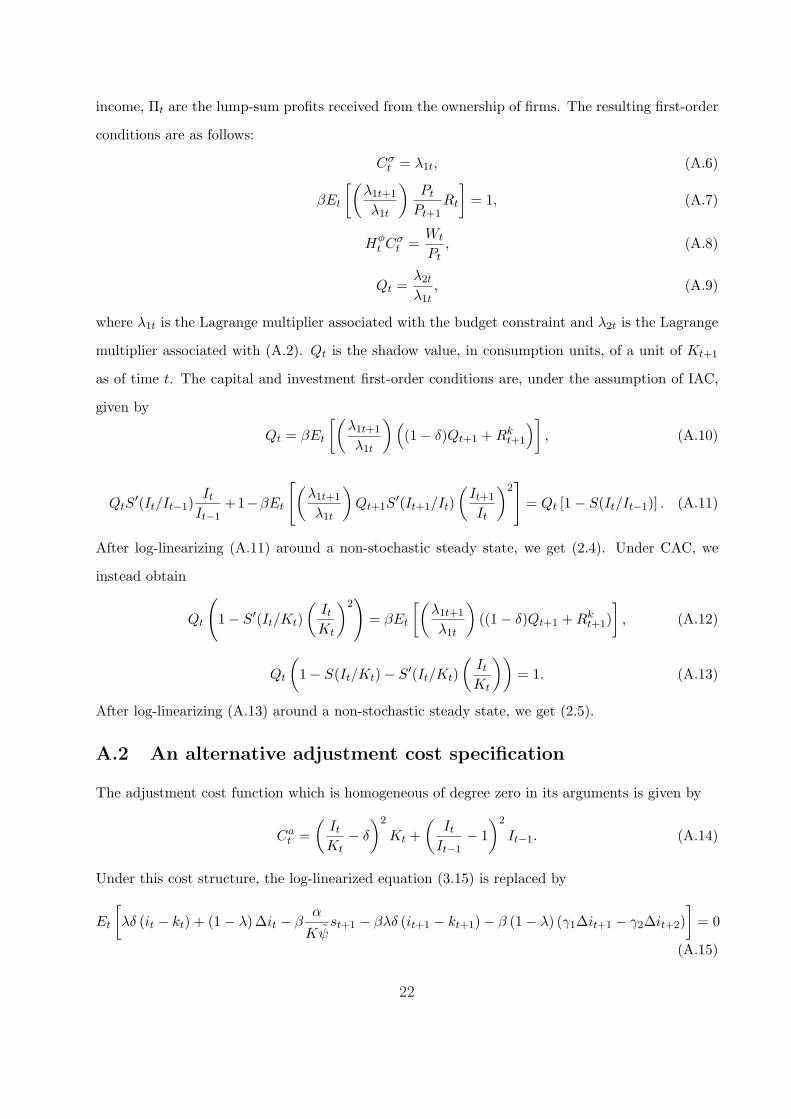
After log-linearizing (A.13) around a non-stochastic steady state, we get (2.5).

A.2 An alternative adjustment cost specification

The adjustment cost function which is homogeneous of degree zero in its arguments is given by

Cat =

(It

Kt− δ

)2

Kt +(

It

It−1− 1

)2

It−1. (A.14)

Under this cost structure, the log-linearized equation (3.15) is replaced by

Et

[λδ (it − kt) + (1− λ)∆it − β

α

Kψst+1 − βλδ (it+1 − kt+1)− β (1− λ) (γ1∆it+1 − γ2∆it+2)

]= 0

(A.15)

22

where γ1 = 1 + (1− δ) , γ2 = β (1− δ) . The difference, compared to (3.15), is the presence of the

steady state value of the capital stock, K. The mapping between the industry and the aggregate

elasticity is modified as

1κ

= − δα

ψ (r + δ)=

α

ψK (r + δ)⇔ ψ =

ψ

δK.

A.3 AR and K statistics

Following Kleibergen (2002), we can represent (3.15) as a limited information simultaneous equation

model

y = Y Θ + ε (A.16)

Y = XΠ + V (A.17)

where y = ikt(≡ it − kt), Y = [∆it ikt+1 skt+1 ∆it+1 ∆it+2] is Tx5,

Θ ≡ [(1− λ)/λδ2 βα/(ψλδ) − β β(λ− 1)(1 + (1− δ))/λδ2 β2(1− λ)(1− δ)/λδ2

]′ is 5x1,

ε is a Tx1 vector of structural errors, X is Txk matrix of instruments, Π is the parameter matrix

for the second equation, and V is Txm matrix of reduced form errors. Under the null hypothesis

H0 : Θ = Θ0, where λ = λ and ψ = ψ and the remaining parameters are calibrated, the AR

statistic is

AR(Θ0) =1k (y − Y Θ0)′PX(y − Y Θ0)1

T−k (y − Y Θ0)′MX(y − Y Θ0)∼ F (k, T − k) (A.18)

where PX = X(X ′X)−1X ′ and MX = I − PX .

The K-statistic is

K(Θ0) =(y − Y Θ0)′PY (Θ0)(y − Y Θ0)1

T−k (y − Y Θ0)′MX(y − Y Θ0)∼ χ2(m) (A.19)

where

PY (Θ0) = Y (Θ0)(Y (Θ0)′Y (Θ0))−1Y (Θ0)′

Y (Θ0) = XΠ(Θ0),

Π(Θ0) = (X ′X)−1X ′[Y − (y − Y Θ0)

sεV (Θ0)sεε(Θ0)

],

sεV (Θ0) =1

T − k(y − Y Θ0)′MXY,

sεε(Θ0) =1

T − k(y − Y Θ0)′MX(y − Y Θ0)

23

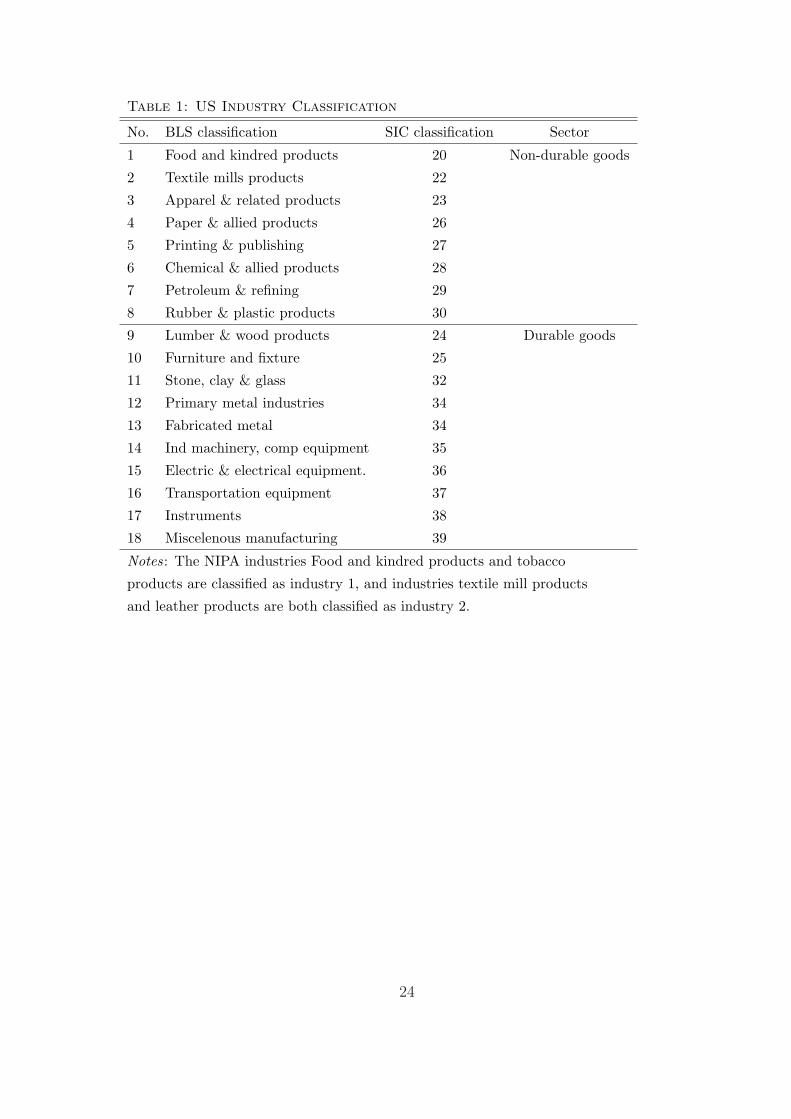
Table 1: US Industry Classification

No. BLS classification SIC classification Sector

1 Food and kindred products 20 Non-durable goods

2 Textile mills products 22

3 Apparel & related products 23

4 Paper & allied products 26

5 Printing & publishing 27

6 Chemical & allied products 28

7 Petroleum & refining 29

8 Rubber & plastic products 30

9 Lumber & wood products 24 Durable goods

10 Furniture and fixture 25

11 Stone, clay & glass 32

12 Primary metal industries 34

13 Fabricated metal 34

14 Ind machinery, comp equipment 35

15 Electric & electrical equipment. 36

16 Transportation equipment 37

17 Instruments 38

18 Miscelenous manufacturing 39

Notes: The NIPA industries Food and kindred products and tobacco

products are classified as industry 1, and industries textile mill products

and leather products are both classified as industry 2.

24

Table 2: Estimation Results (Non-Linear Specification)

Parameters J

Industry α ψ λ p-value

1. -0.08*** 0.23*** 1.00*** 0.86

(0.00) (0.01) (0.00)

2. -0.45*** -0.32 0.93*** 0.94

(0.01) (0.71) (0.13)

3. -0.22*** 0.98*** 1.00*** 0.94

(0.00) (0.19) (0.00)

4. -0.13*** 0.04 0.96*** 0.85

(0.00) (0.04) (0.00)

5. -0.09*** 0.14* 1.00*** 0.87

(0.00) (0.08) (0.02)

6. -0.07*** 0.06*** 0.97*** 0.74

(0.00) (0.02) (0.00)

7. -0.09*** -0.08 1.00*** 0.98

(0.00) (0.10) (0.01)

8. -0.12*** 0.19*** 0.97*** 0.95

(0.00) (0.03) (0.00)

9. -0.22*** 0.10 1.00*** 0.92

(0.01) (0.24) (0.07)

10. -0.26*** -0.12 0.92*** 0.84

(0.01) (0.32) (0.17)

11. -0.23*** 0.05 1.00*** 0.92

(0.00) (0.04) (0.05)

12. -0.13*** 0.27*** 1.00*** 0.95

(0.00) (0.03) (0.00)

13. -0.08*** 0.25*** 1.00*** 0.93

(0.00) (0.02) (0.00)

14. -0.06*** 0.17*** 0.96*** 0.83

(0.00) (0.01) (0.00)

15. -0.09*** 0.29*** 0.97*** 0.85

(0.01) (0.07) (0.00)

16. -0.09*** 0.26*** 0.95*** 0.72

(0.00) (0.05) (0.00)

17. -0.10*** 0.16*** 1.00*** 0.98

(0.00) (0.03) (0.01)

18. -0.34*** 0.06*** 0.98*** 0.84

(0.01) (0.29) (0.10)

Notes: Estimates of Euler equation (3.8). Instruments:

lags 2 to 6 of oil-shock dummies and the innovation in

federal defense spending. Standard errors in parenthesis

* significant at 10-percent; ** significant at 5-percent;

*** significant at 1-percent.

25

Table 3: Estimation Results (Linearized Specification) with Weak Instrument Diagnostics and

Identification Robust Tests

Parameters J partial-R2 AR K

Industry ψ λ p-value R2p(st+1) R2

p(ikt+1) R2p(∆it+1) R2

p(∆it+2) p-value p-value

1. 0.59*** 1.00*** 0.90 0.14 0.08 0.09 0.24 0.78 0.72

(0.18) (0.00)

2. 2.68*** 1.00*** 0.96 0.07 0.26 0.21 0.15 0.30 0.25

(0.82) (0.00)

3. 0.08 1.00*** 0.88 0.06 0.30 0.21 0.24 0.45 0.19

(0.22) (0.02)

4. 0.93*** 1.00*** 0.83 0.26 0.18 0.36 0.14 0.11 0.01

(0.20) (0.00)

5. 0.18 1.00*** 0.82 0.08 0.12 0.13 0.14 0.20 0.21

(0.22) (0.00)

6. 0.40*** 1.00*** 0.79 0.31 0.23 0.10 0.15 0.43 0.44

(0.15) (0.00)

7. 1.64*** 1.00*** 0.86 0.35 0.23 0.23 0.18 0.27 0.13

(0.55) (0.00)

8. -0.27 1.00*** 0.84 0.05 0.09 0.15 0.13 0.58 0.75

(0.36) (0.02)

9. -0.46 1.00*** 0.89 0.10 0.29 0.38 0.10 0.12 0.18

(0.42) (0.00)

10. 1.92*** 1.00*** 0.88 0.09 0.22 0.07 0.08 0.17 0.12

(0.39) (0.00)

11. 1.00*** 1.00*** 0.94 0.10 0.17 0.24 0.09 0.07 0.04

(0.35) (0.00)

12. 2.52*** 1.00*** 0.96 0.15 0.13 0.11 0.10 0.04 0.00

(0.85) (0.00)

13. 0.59*** 1.00*** 0.98 0.03 0.06 0.07 0.08 0.21 0.71

(0.18) (0.00)

14. 0.50*** 1.00*** 0.91 0.16 0.13 0.14 0.09 0.03 0.03

(0.15) (0.00)

15. 0.14** 1.00*** 0.89 0.12 0.05 0.11 0.13 0.25 0.37

(0.06) (0.00)

16. 0.10 1.00*** 0.80 0.05 0.04 0.09 0.15 0.22 0.47

(0.12) (0.01)

17. 0.50*** 1.00*** 0.98 0.12 0.23 0.24 0.23 0.85 0.60

(0.12) (0.00)

18. 0.77 1.00*** 0.94 0.06 0.24 0.19 0.19 0.05 0.06

(0.57) (0.00)

Notes: Estimates of Euler equation (3.13). Instruments: lags 2 to 6 of oil-shock dummies and the

innovation in federal defense spending. Standard errors in parenthesis: * significant at 10-percent;

** significant at 5-percent; *** significant at 1-percent.

26

Table 4: Estimation Results (Non-Linear Specification) with λ Constrained

Investment Adjustment Costs (λ=0) Capital Adjustment Costs (λ=1)

Parameters J Parameters J

Industry α ψ p-value α ψ p-value

1. -0.06*** 0.00 0.90 -0.06*** 0.01 0.90

(0.00) (0.00) (0.00) (0.10)

2. -0.46*** 0.01*** 0.93 -0.46*** 3.26*** 0.94

(0.00) (0.00) (0.00) (0.92)

3. -0.19*** 0.01*** 0.91 -0.20*** 1.38*** 0.93

(0.00) (0.00) (0.00) (0.00)

4. -0.12*** -0.00 0.91 -0.12*** -0.01 0.90

(0.00) (0.00) (0.00) (0.07)

5. -0.09*** 0.001*** 0.90 -0.09*** 0.19** 0.90

(0.00) (0.00) (0.00) (0.09)

6. -0.07*** -0.001* 0.82 -0.07*** -0.08** 0.83

(0.00) (0.00) (0.00) (0.04)

7. -0.09*** -0.00 0.97 -0.09*** -0.04 0.97

(0.00) (0.00) (0.00) (0.10)

8. -0.102*** -0.00 0.88 -0.10*** -0.20*** 0.89

(0.00) (0.00) -(0.00) (0.08)

9. -0.21*** 0.00 0.97 -0.21*** 0.26* 0.97

(0.00) (0.00) (0.00) (0.15)

10. -0.24*** -0.01*** 0.82 -0.28*** -0.30 0.87

(0.00) (0.00) ()0.00 (0.58)

11. -0.22*** -0.00 0.94 -0.22*** 0.10 0.94

(0.00) (0.00) (0.00) (0.19)

12. -0.10*** 0.001*** 0.92 -0.12*** 0.15 0.87

(0.00) (0.00) (0.00) (0.10)

13. -0.06*** 0.001*** 0.90 -0.06*** 0.37* 0.87

(0.00) (0.00) (0.00) (0.21)

14. -0.04*** 0.001*** 0.93 -0.04*** 0.22*** 0.93

(0.00) (0.00) (0.00) (0.09)

15. -0.04*** 0.00 0.93 -0.04*** -0.01 0.94

(0.00) (0.00) (0.00) (0.06)

16. -0.07*** 0.00 0.81 -0.07*** 0.25*** 0.91

(0.00) (0.00) (0.00) (0.03)

17. -0.09*** -0.00 0.90 -0.09*** -0.03 0.90

(0.00) (0.00) (0.00) (0.12)

18. -0.34*** -0.00 0.90 -0.34*** -0.06 0.90

(0.00) (0.00) (0.00) (0.31)

Notes: Estimates of Euler equation (3.8). Instruments: lags 2 to 6 of oil-shock dummies

and the innovation in federal defense spending. Standard errors in parenthesis: * significant

at 10-percent; ** significant at 5-percent; *** significant at 1-percent.

27