investment gaps in idb borrowing...

Graduate Institute of International and Development Studies

International Economics Department

Working Paper Series

Working Paper No. HEIDWP03-2018

Investment Gaps in IDB Borrowing Countries

Francesca CastellaniInter-American Development Bank

Marcelo OlarreagaUniversity of Geneva and CEPR

Ugo PanizzaThe Graduate Institute Geneva and CEPR

Yue ZhouThe Graduate Institute Geneva

Chemin Eugene-Rigot 2P.O. Box 136

CH - 1211 Geneva 21Switzerland

c©The Authors. All rights reserved. Working Papers describe research in progress by the author(s) and are published toelicit comments and to further debate. No part of this paper may be reproduced without the permission of the authors.

1

Investment Gaps in IDB Borrowing Countries

Francesca Castellani Marcelo Olarreaga

Ugo Panizza Yue Zhou*

Abstract We estimate public investment gaps in a sample of developing countries using a public investment demand function. We then use GDP per capita projections, forecasts of structural transformation, and three SDG targets (poverty, infant mortality and lower secondary school completion) to predict public investment needs in 2030 among IDB borrowing countries. Our estimates suggest that in 2014 the total public investment gap of IDB borrowers was close to $170 billion (3.1 percent of the Region’s GDP) and that the gap is expected to surpass $717 billion (6.3 percent of the Region’s GDP) by 2030 if the SDGs were to be reached. JEL classification: H54, H63, O16, O54 Keywords: Investment gaps, Latin America, SDG

* We are grateful to Alexandre Meira da Rosa, Gaston Astesiano, and Rúben Cuevas for helpful comments. The views set out in this study are those of the authors and do not necessarily reflect the official opinion of the Inter-American Development Bank. The usual caveats apply. Castellani is with the Inter-American Development Bank ([email protected]); Olarreaga is with the University of Geneva and CEPR ([email protected]); Panizza is with the Graduate Institute Geneva and CEPR ([email protected]); and Zhou is with the Graduate Institute Geneva ([email protected]).

2

1 Introduction

At the Rio+20 conference, which took place in Rio de Janeiro in June 2012, Member States called

for a prioritization of the sustainable development agenda. The conference eventually led to the

2015 UN Sustainable Development Summit and to the launch, on January 1st 2016, of the 2030

Agenda for Sustainable Development and its 17 Sustainable Development Goals (SDGs).

Achieving the SDGs will require improved policies and governance and higher levels of

public and private investment. Estimates of annual financing needs for meeting the SDGs range

between $1.5 and $2.5 trillion. This note contributes to the discussion by estimating public

investment gaps for a large sample of developing and emerging market countries and by describing

a simple methodology for incorporating SDGs target in these gap estimates. The note also presents

a detailed discussion of investment gaps in IDB borrowing countries.

We start by assessing public investment demand in a sample of developing and emerging

economies and then compute the public investment gap in each country as the difference between

estimated public investment demand and observed public investment. Next, we use our model and

GDP projections to forecast investment gaps up to 2030. Finally, we use the relationship between

public investment and selected SDGs (i.e. poverty ratios, child mortality rate under the age of 5,

and lower secondary school completion), to assess the public investment needed to reach these

targets.

As there is evidence that public investment is a driver of economic growth (Abiad et al.

2016), policies that promote public investment can deliver high returns in terms of economic

development.1 Peter Drucker famously stated that what gets measured gets done. Hence, measuring

public investment gaps is necessary for implementing policies aimed at closing these gaps.

Quantifying the current and future needs for public investment can also help international financial

institutions predict future demand, and target lending to countries that need it the most. We also

1 Public investment has both direct and indirect effects on economic growth. The indirect effects are linked to the complementarities between public and private investment (Dreger and Reimers, 2016). There, however, also authors that found that public investment crowds out private investment (Afonso and St. Aubyn, 2016).

3

show that public investment can promote equitable growth by helping eradicate extreme poverty,

reducing child mortality, and promoting education, as requested by the SDGs.

We find that public investment gaps vary significantly across regions. While the East Asia

and Pacific region overinvests to the tune of 5.5 percent of GDP, all other developing regions

display large investment gaps. In Latin America and the Caribbean, the investment gap was above

3 percent of GDP in 2014 and expected to reach 4.4 percent of GDP in 2030. If we factor in the

public investment needed to eradicate extreme poverty, as requested by the SDGs, the 2030 public

investment gap among IDB borrowing members reaches 5 percent of GDP or $524 billion. If we

were to add the resources needed to reach the targets for child mortality under the age of 5 and

secondary school enrollment in 2030, the gap would reach 5 percent of GDP or $566 billion. If we

were to add to the poverty target, the infant mortality and the lower secondary completion targets,

the gaps would reach 6.6 percent of GDP or $717 billion.

We are aware that there are issues with data quality and with our empirical methodology.

One key problem has to do with the measurement of public investment. In measuring investment,

we normally assume that every dollar spent will increase the value of the capital stock (investment

is often referred to as “gross fixed capital formation”). This assumption might be less realistic for

public investment, especially in countries with poor institutions, high corruption, and low

bureaucratic quality (Pritchett, 2000). The second issue relates to the endogeneity problem and to

our ability to measure the “demand” for public investment. We discuss this issue in Section 3

below. These caveats notwithstanding, our estimations are useful in providing a benchmark and in

guiding policies to promote greater public investment, especially in countries with large public

investment gaps.

We are not the first to assess public investment needs and their associated investment gaps.

To estimate investment demand, we build on Fay (2000), Fay and Yepes (2003), and Ruiz-Nuñez

and Wei (2015) but, unlike these authors, we focus on total investment expenditure rather than

estimating separate demand equations for different types of infrastructure. By focusing on total

investment expenditure, we can obtain direct estimates of the monetary value of investment

demand without the need of making assumptions on the unit cost of different infrastructure

4

projects.

The launch of the Millennium Development Goals in 2000 led to a wave of “needs

assessment” for MDG investment areas (UN Millennium Project 2005, MDG Africa Steering

Group 2008, Bourguignon et al. 2008) and similar assessments have also been developed for the

SDGs (for a review, see Schmidt-Traub and Sachs, 2015). These studies are difficult to compare

and aggregate because they propose different country coverage, methodologies and assumptions

and mix quantitative estimates with expert assessments (see Schmidt-Traub, 2015 for an attempt

to aggregate different SDG estimates). Our methodology is instead purely quantitative and uniform

across countries. It can thus be a useful complement, albeit not a substitute, to needs assessments

based on expert judgment.

The reminder of the paper is organized as follows. Section 2 provides descriptive statistics

on private, public and total investment and capital stocks across developing regions as well as

among individual IDB borrowing countries. In section 3 we present the empirical methodology

used to estimate public investment gaps, and present the estimates for current and projected public

investment gaps. Section 4 describes the methodology used to predict the public investment needed

to reach the selected SDG targets and provides estimates by region and IDB borrowing countries.

Section 5 focuses on the role of the IDB. Section 6 concludes.

2 Investment and capital stock in developing countries

The average capital stock of Latin American and Caribbean countries (LAC) declined from nearly

250 percent of GDP in 1990 to 190 percent of GDP in 2010 and recovered slightly to 200 percent

of GDP over 2010-15 (Table 1, all averages are weighted by GDP measured in 2000 PPP US

dollars). 2 This nearly 20 percent decline is in contrast with what happened in the East Asia and

Pacific (EAP) region, where the capital stock increased from 180 percent of GDP in 1990 to over

2 By LAC we mean IDB borrowing members: Argentina, Bahamas, Barbados, Belize, Bolivia, Brazil, Chile, Costa Rica, Dominican Republic, Ecuador, El Salvador, Guatemala, Guyana, Haiti, Honduras, Jamaica, Mexico, Nicaragua, Panama, Paraguay, Peru, Suriname, Trinidad and Tobago, Uruguay and Venezuela. For data sources, see Data Appendix.

5

250 percent in 2015. While in 1990 Latin America was the developing region with the largest

capital stock-to-GDP ratio, by 2000 it had been surpassed by both EAP and Eastern Europe and

Central Asia (ECA). By 2015 LAC ranked second, lagging 20 percent behind EAP where

investment rates remained high throughout the period.

More in general, the decline in capital stock observed in Latin America and the Caribbean

over 1990-2015 is not at odds with the trends in ECA, Middle East and North Africa (MNA) or

Sub-Saharan Africa (SSA). In fact, in 2015 the average capital stock ratio in LAC was similar to

the developing country average, which

stood at around 205 percent. In terms of

the median country, however, the decline

in the capital stock in the LAC region was

more pronounced than that observed in

other regions. In 2015, the LAC median

capital stock was the second lowest among

developing regions.

In terms of private capital-to-GDP

ratios, in 2015 LAC was the region with

the highest average (Table 2). However,

East Asia and Pacific has been catching up

rapidly. Its private capital stock-to-GDP

ratio increased from 79 percent in 1990 to

134 percent in 2015, while the private capital stock-to-GDP ratio of the LAC region decreased

from 165 percent to 138 percent. If this trend continues, EAP will soon surpass LAC. While the

average private capital stock-to-GDP ratio of the LAC region is much larger than in ECA, MNA,

South Asia (SAS), and SSA, all regions have similar medians that oscillate between 104 percent

and 112 percent of GDP.

The LAC region performs particularly poorly in term of public capital. In 2015, the average

public capital-to-GDP ratio in LAC (Table 3) was only 62 percent: 40 percent smaller than the ratio

Table 1: Total Capital Stock to GDP ratio (%) Region 1990 2000 2010 2015 Mean EAP 182 222 226 253 ECA 188 235 161 158 LAC 246 217 191 200 MNA 217 175 167 186 SAS 156 158 159 168 SSA 235 205 158 167 Median

EAP 190 221 222 220 ECA 126 167 167 166 LAC 193 196 170 166 MNA 230 203 174 218 SAS 144 152 148 157 SSA 212 211 183 199

Source: Authors’ calculations using IMF’s Investment and Capital stock dataset where capital stocks and GDP are measured in 2000 PPP USD dollars. All averages are weighted by GDP. East Asia and Pacific (EAP), Middle East and North Africa (MNA); Eastern Europe and Central Asia (ECA); Latin America and the Caribbean (LAC), South Asia (SAS) and Sub-Saharan Africa (SSA)

6

observed in MNA (a region with a large public capital stock and a small stock of private capital);

half the average ratio in the EAP region (which has high private and public capital), and even

smaller than the average ratio in SSA. Only SAS and ECA show lower levels of public capital.

Over 1990-2015, both public and

private capital stocks declined in the

LAC region. However, public

investment declined more rapidly than

private investment. As a consequence,

the average share of public capital stock

over total capital declined from 33 to 31

percent between 1990 and 2015 (Table

4). While LAC’s share of public capital

in total capital is much smaller than the

share observed in MNA, EAP or even

SSA, the public capital share in LAC is

similar to the end of 2015 shares in SAS

and ECA. However, these two regions

Table 2: Private Capital Stock to GDP ratio (%) Region 1990 2000 2010 2015 Mean

EAP 79 97 106 134 ECA 147 177 115 112 LAC 165 144 131 138 MNA 92 81 80 87 SAS 74 86 101 112 SSA 140 122 95 101 Median

EAP 79 109 117 112 ECA 82 118 110 112 LAC 135 128 116 109 MNA 63 65 93 104 SAS 79 90 104 105 SSA 108 110 94 105 Source: Authors’ calculations using IMF’s Investment and Capital stock dataset where capital stocks and GDP are measured in 2000 PPP USD dollars. All averages are weighted by GDP.

Table 3: Public Capital Stock to GDP ratio (%) Region 1990 2000 2010 2015 Mean

EAP 103 124 120 120 ECA 41 58 45 46 LAC 81 72 59 62 MNA 124 94 86 100 SA 82 72 58 56 SSA 95 83 63 66 Median

EAP 51 60 66 65 ECA 35 50 44 45 LAC 66 59 58 62 MNA 109 81 80 94 SAS 59 64 55 52 SSA 77 94 74 87 Source: Authors’ calculations using IMF’s Investment and Capital stock dataset where capital stocks and GDP are measured in 2000 PPP USD dollars. All averages are weighted by GDP.

Table 4: Public Capital Stock/Total Capital Stock (%) Region 1990 2000 2010 2015 Mean



Source: Authors’ calculations using IMF’s Investment andCapital stock dataset where capital stocks and GDP are measured in 2000 PPP USD dollars. All averages are weighted by GDP.

7

had different trends. SAS has a declining share of public capital because private capital grew very

rapidly and ECA has an increasing share of public capital because private capital declined rapidly

during the period.

High public investment shares in East Asia and low public investment shares in Latin

America are partly driven by outliers (Table 3, bottom panel). The median Latin American country

has a public investment share, which is lower than the MNA and SSA medians, but well above the

medians of EAP, ECA, and SAS.

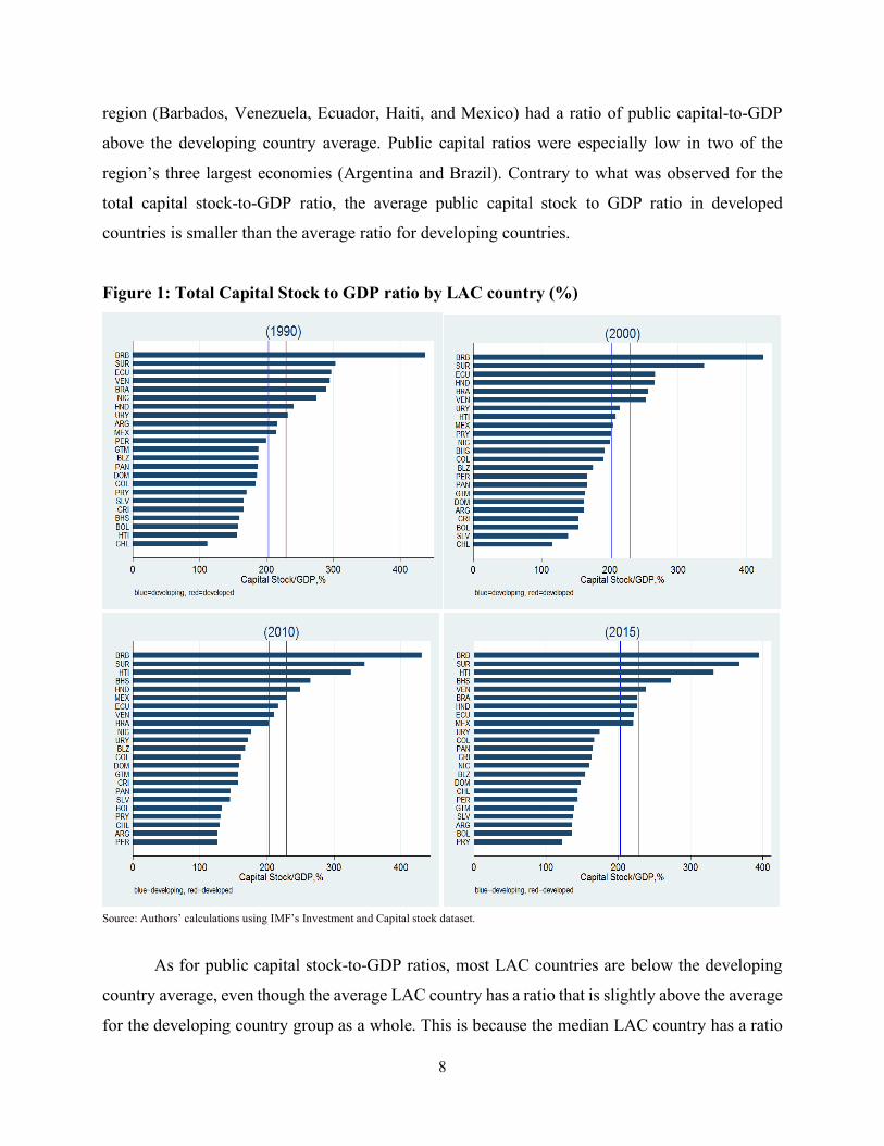
The large deviation between the average and median measures for the Latin American

capital stock suggests that there is substantial dispersion and skewness in the cross–country

distribution of this indicator. Figure 1 provides total capital stock-to-GDP ratios for LAC countries

in 1990, 2000, 2010, and 2015.

In 1990, 13 countries in the region (out of 23 for which data is available) displayed a total

capital stock-to-GDP ratio below the developing country average (the blue line in Figure 1). By

2000, 15 countries in the region had capital stock-to-GDP ratios below the developing country

average.

In 1990, 8 countries in the region exhibit a capital stock-to-GDP ratio above the advanced

economies average (the red line in Figure 1). By 2015 only five countries had a capital ratio above

that of the average advanced economy. Among these five countries, there are two high-income

small Caribbean countries (Bahamas and Barbados), one middle-income small Caribbean country

(Suriname), one low-income country (Haiti), and only one of the largest seven economies in the

region (Venezuela). As to the large countries in the region, Brazil and Mexico had capital stock to

GDP ratio above the developing country average; and Argentina, Chile, Colombia, and Peru low

capital stocks.

Figure 2 confirms that public capital explains the relatively low capital stock-to-GDP ratio

in the LAC region. The average developing country has a public capital-to-GDP ratio of about 90

percent; the average in LAC is just above 60 percent (Table 2). In 2015, only 5 countries in the

8

region (Barbados, Venezuela, Ecuador, Haiti, and Mexico) had a ratio of public capital-to-GDP

above the developing country average. Public capital ratios were especially low in two of the

region’s three largest economies (Argentina and Brazil). Contrary to what was observed for the

total capital stock-to-GDP ratio, the average public capital stock to GDP ratio in developed

countries is smaller than the average ratio for developing countries.

Figure 1: Total Capital Stock to GDP ratio by LAC country (%)

Source: Authors’ calculations using IMF’s Investment and Capital stock dataset.

As for public capital stock-to-GDP ratios, most LAC countries are below the developing

country average, even though the average LAC country has a ratio that is slightly above the average

for the developing country group as a whole. This is because the median LAC country has a ratio

9

that is a lower than the LAC average and the developing country averages. Caribbean countries

tend to be at the top of the distribution in terms of private capital-to-GDP ratios. Venezuela, instead,

which was at the top of the distribution in terms of public capital stock and total capital stocks, is

at the bottom of the distribution in terms of private capital-to-GDP ratio. The same is true, although

to a lesser extent, for Bolivia whose very low private capital stock is only marginally compensated

by its stock of public capital. Argentina moved from having one of the largest private capital stocks

in 1990 to the bottom half of the distribution in 2015.

The share of public to total capital stock in LAC countries tends to be below the average

for developing countries at 43 percent (Figure 4). In 2015, only Venezuela, Bolivia, Barbados,

Ecuador, and Belize had a share that was above the developing country average. Eleven out of the

twenty-four LAC countries in our sample have a share of public capital that is lower than the

average share among developed countries. This group includes some large countries such as

Argentina and Brazil.

The three largest countries in the region present interesting cases. Brazil’s low public capital

share is driven by a large private capital stock (the largest in the region if small Caribbean countries

are excluded, Figure 3) and a small public capital stock (in the bottom 30 percent of the regional

distribution). Argentina’s, private and public capital are below average, but public capital is even

smaller than private capital, putting the country near the bottom of the distribution of the share of

public capital. Finally, Mexico has above average public and private capital ratios, but a relatively

higher public capital ratio.

10

Figure 2: Public Capital Stock to GDP ratio by LAC country (%)


11

Figure 3: Private Capital Stock to GDP ratio by LAC country (%)


12

Figure 4: Share of Public Capital Stock in Total Capital Stock by LAC country (%)


Tables 5 to 8 reproduce Tables 1 to 4 but for investment flows. They show regional patterns

similar to those described above. However, contrary to the capital stock that has been declining in

LAC over the last three decades, total investment-to-GDP ratios have increased from of 14 to 19

percent (Table 5). In fact, investment increased in most developing regions (the exception is ECA

where investment collapsed in the 1990s) and throughout the period the total investment-to-GDP

ratio in LAC was similar to that observed in most developing regions. The exception is EAP, which,

by 2015, had a total investment-to-GDP ratio twice as large as that of LAC.

13

Table 5: Total Investment-to-GDP ratio (%) Region 1990 2000 2010 2015 Mean



Source: Authors’ calculations using IMF’s Investment and Capital stock dataset where capital stocks and GDP are measured in 2000 PPP USD dollars.

Table 6: Public Investment-to-GDP ratio (%) Region 1990 2000 2010 2015




Table 7: Private Investment-to-GDP ratio (%) Region 1990 2000 2010 2015 Mean




Table 8: Public Investment/Total Investment (%) Region 1990 2000 2010 2015 Mean




In terms of public investment-to-GDP ratios, the patterns are again similar to the ones

observed for the stock of public capital. Investment rates remained relatively stable during the

period and LAC is the region with the second lowest public investment-to-GDP ratio (after ECA,

Table 6). The share of private investment in GDP increased throughout the period from 10 percent

in 1990 to 15 percent by 2015 (Table 7) confirming that it is private investment that drove the

14

increase in total investment in LAC between 1990 and 2015. The average country in LAC has a

private investment-to-GDP ratio that is similar to that of other regions. The exception, again, is

EAP where the private investment-to-GDP ratio is 11 percentage points (corresponding to 60

percent of the investment ratio in LAC) larger than in LAC.

Figure 5: Total Investment-to-GDP ratio by LAC country (%)


LAC’s share of public over total investment declined by a third between 1990 and 2015

(Table 8). In 2015, the share of public investment over total investment in MNA countries was

twice the LAC share and EPA and SSA had average shares at least one third larger than that of

LAC. ECA and SAS had instead shares of public investment in total investment similar to LAC’s

average.

Within LAC the patterns in terms of investment flows are also similar to the ones observed

for capital stocks (Figures 5-8). In 2015, all but five LAC countries (Panama, Bahamas, Barbados,

15

Haiti and Suriname) had a total investment-to-GDP ratio that was below the developing country

average of about 20 percent of GDP (the blue line in Figure 5).

Figure 6: Public Investment-to-GDP ratio by LAC country (%)


In terms of public investment-to-GDP ratio, in 2015 there were only four LAC countries

with a ratio above the developing country average: Bolivia, Haiti, Venezuela, and Ecuador (Figure

6).3 In 2015, Guatemala, Bahamas, El Salvador, and Brazil were at the bottom of the distribution

with ratios below 2 percent.

In the case of private investment, twelve LAC countries were above the developing country

average in 2015 (Figure 7). Among the countries with a high share of private investment in GDP

there are large countries such as Brazil and Chile.

3 The average public investment-to-GDP ratio for developing countries tends to be larger than the average for developed countries, whereas in terms of total investment-to-GDP ratio the averages for developed and developing countries are similar.

16

Figure 7: Private Investment-to-GDP ratio by LAC country (%)


In 2015, only five LAC countries had a share of public investment in total investment larger

than the developing country average: Venezuela, Bolivia, Belize, Ecuador, and Haiti (Figure 8).

These descriptive statistics suggest that the share of public investment in total investment could be

significantly increased in 18 countries in the region.

17

Figure 8: Share of Public Investment in Total Investment by LAC country (%)


To test whether countries with a small capital stock are catching up with countries with

larger ones, we regressed the investment-to-GDP-ratio in 2015 over the capital stock-to-GDP ratio

in the same year. We found a positive correlation (Figure 9a) suggesting that investment is actually

higher in countries with a larger capital stock (each dot in the figure is a country, LAC countries

are labeled with their three-letter ISO code). The point estimate of 0.065 indicates that a 100 percent

of GDP increase in the capital stock is associated with a 6.5 percent of GDP increase in the

investment rate. This is about one percentage point larger than the average depreciation rate used

to build the capital stock.4 Therefore, the regression indicates that, on average, there is a small

divergence. Countries with a higher capital stock invest more and the investment differential is

4 The IMF estimates that public capital depreciation for low and middle-income countries ranges between 2.5 percent and 3.6 % and private capital depreciation for low and middle countries ranges between 4.2 percent and 8.3 percent. About two-thirds of the countries include in the regressions of Figure 6a are middle income, yielding a public capital depreciation rate of 3.2 percent and a private capital depreciation rate of 7 percent. With a public capital share of 35 percent, we obtain an average depreciation rate of 5.5 percent

18

slightly larger than the depreciation differential. Countries that are above or on the regression line

(such as Suriname, Panama, Bahamas, and Chile) are moving towards a higher capital stock and

countries farther below the regression line (such as Barbados, Trinidad and Tobago, and

Venezuela) are moving towards a lower capital stock.

Figure 9: Investment rates and capital stock a. Total investment

c. Public investment

b. Private investment

Focusing on private capital, we find a coefficient of 0.10 (Figure 9b), which is higher than

the assumed depreciation rate for private capital of about 7 percent. This implies that there is

divergence, as the increase in investment associated with a larger capital stock is larger than what

is needed to compensate for depreciation. The figure suggests that Suriname and Panama are

moving towards larger private capital and Haiti, Venezuela, and Trinidad and Tobago are moving

towards a smaller private capital stock.

19

Finally, Figure 9c shows a divergence in public capital, but at a much smaller rate with

respect to public capital (the regression’s coefficient implies a 4.8 percent elasticity and the

estimated public capital depreciation rate is 3.2 percent). Regression’s results suggest that

Venezuela, Haiti, and Bolivia are moving towards a larger stock of public capital and Trinidad and

Tobago, Barbados, Mexico and Guatemala are moving toward lower stocks of public capital.

The IMF data used so far focus on total investment. Cross-country data on infrastructure

investment from the Global Infrastructure Hub are only available for a small number of countries

and start in 2010. For those countries, the pattern is similar to that for total investment. In 2015,

LAC infrastructure investment represents on average 2.6 percent of GDP, well below the 5 percent

infrastructure investment needs estimated by Serebrisky et al. (2015). In EAP and SSA the average

is above 5 percent, 3.7 percent in SAS and 3.0 percent in MNA. Overall, LAC’s infrastructure

investment is much lower than in the developing world average.

The Latin American Development Bank (CAF) the Economic Commission for Latin

America and the Caribbean (ECLAC) and the Inter-American Development Bank (IDB) have

assembled a detailed dataset on infrastructure investment (INFRALATAM) covering 18 countries

in Latin America and the Caribbean. Figure 10 corroborates our previous results, suggesting that

most countries in the regions have low investment levels. Specifically, in 2015, only 4 countries in

the region (Bolivia, Peru, Colombia and Nicaragua) invested in infrastructure more than the

average developing economy. The figure also shows that infrastructure investment is particularly

low in the Region’s three largest economies (Brazil, Argentina, and Mexico).

20

Figure 10: Infrastructure investment by LAC country (%)

Source: Authors’ calculations using INFRALATAM data.

Infrastructure quality also matters. Even if the level of total or public investment in LAC is

relatively low, it may be that the

quality or the efficiency of total

and public investment is higher

in LAC than in other regions.

To check this, we use World

Economic Forum data to

calculate average infrastructure

efficiency by region in 2014

(Table 9). 5 The first column

shows the raw index and the

second the index conditional on GDP per capita (these are the residuals of a regression of the

infrastructure index over the log of GDP per capita).

5 See http://www3.weforum.org/docs/GCR2016-2017/05FullReport/TheGlobalCompetitivenessReport2016-2017_FINAL.pdf

Table 9: Infrastructure Efficiency, 2014

Region Infrastructure quality 2014

Infrastructure quality conditional on GDP per capita

East Asia & Pacific 4.4 0.3 Europe & Central Asia 4.4 0.3 Latin America & Caribbean 3.5 -0.6 Middle East & North Africa 4.6 0.5 South Asia 3.7 -0.4 Sub-Saharan Africa 3.4 -0.7

Source: Authors’ calculations using WEF’s Infrastructure efficiency data dataset and World Bank’s WDI for GDP per capita. The WEF infrastructure quality index ranges from 1 to 7. After conditioning on GDP per capita the average of the residual across all countries is equal to zero.

21

The results suggest that infrastructure quality in Latin America is not better than in the rest

of the developing world. If we exclude Sub-Saharan Africa, infrastructure quality in Latin America

tends to be lower than other developing regions, with a larger difference if we control for GDP per

capita. Table 9 shows that, in Latin America, investment in infrastructure lacks both in terms of

quantity and quality.

Figure 11: Infrastructure efficiency in LAC

Source: Authors’ calculations using WEF’s infrastructure efficiency data and World Bank’s WDI for GDP per capita. The (unconditional) infrastructure quality index varies between 1 and 7.

Within LAC, infrastructure quality varies across countries, with relatively high

infrastructure quality (but still below the developed country average) in Barbados, Panama, Chile,

Trinidad and Tobago, El Salvador, Guatemala, Mexico and Jamaica. The quality of infrastructure

is instead low in Paraguay, Venezuela and Haiti (Figure 11). We obtain the same ranking if we

condition for GDP per capita. Among South American countries, only Chile has an infrastructure

quality index above the developing country average.

3 Estimating public investment gaps

In this section, we estimate investment gaps for Latin America and the Caribbean and compare

them with gaps in other developing regions. As a first step, we estimate public investment demand

and compare it with actual investment. Next, we project future investment demand and compare it

with a business as usual benchmark. Our approach builds on the methodology of Fay (2000) and

Ruiz-Nuñez and Wei (2015). These authors first estimate the demand for different types of

22

infrastructure by regressing the stock of existing infrastructure on lagged infrastructure stock, GDP

per capita, the sectorial composition of GDP, and a set of country fixed effects. Next, they use

projected GDP per capita growth to estimate future demand for infrastructure in each country and

give a dollar value to these projections by making assumptions on the cost of production of different

infrastructure projects. While we use a similar strategy, we recognize that there are three issues

with the existing methodology.

First, estimating separate demand equations for different types of infrastructure overlooks

their complementarities, for example, between access to electricity and access to sanitation.

Moreover, public money is fungible and governments face a budget constraint and tradeoffs. The

decision to invest in a certain type of public infrastructure requires an evaluation of its opportunity

costs in terms of other types of public expenditure or, as minimum, alternative investment projects.

It is also methodological complicated to back up the monetary value of investment demand from

regressions that do not include the monetary value of infrastructure investment.6 Additionally, data

availability is limited. Hence, demand estimates for different types of infrastructure are based on

different samples. For instance, in Ruiz-Nuñez and Wei (2015), 96 countries (for a total of 926

observations) have available data for electric generation capacity, but only 57 countries (and 107

observations) for port infrastructure.

Second, existing empirical exercises are based on a business as usual scenario as they

assume that future growth is equal to projected growth. Hence, they do not incorporate the idea

that countries may be trying to meet certain development goals that may require higher public

investment.

Finally, there are econometric problems with the estimation of a fixed effects model in the

presence of a lagged dependent variable. There is also an endogeneity problem, as it is not clear

whether the estimates of Ruiz-Nuñez and Wei (2015) capture demand or supply effects.

6 Ruiz-Nuñez and Wei (2015) estimate models for: telephones subscribers per 1,000 persons; Kilometers of paved roads per squared kilometer of land area; Kilometers of unpaved roads per squared kilometer of land area; Kilometers of rail per 1000 persons; KW of installed electricity generation capacity per capita; Percentage of households with access to electricity; Percentage of households with access to water and sanitation; Percentage of households with access to sanitation; Percentage of households with access to wastewater treatment.

23

In order to address the first issue, we do not estimate equations for different types of infrastructure,

but we focus on total public-sector investment. This strategy allows us to use data covering up to

156 countries and provides direct predictions for investment-to-GDP ratios, which can be easily

converted in dollar values using GDP data. We then compute investment gaps by comparing the

estimated investment demand with realized investment.

We address the second issue by estimating the conditional correlation between public

investment and an indicator of extreme poverty. Next, we use the SDG target to compute the

amount of public investment necessary to close the gap between the current value of extreme

poverty and the SDG goal. Finally, we add this amount of public investment to the estimated

investment demand described above.

While we cannot fully address the endogeneity issue, we use the standard system GMM

estimator of Arellano and Bover (1995) and Blundell and Bond (1998) to deal with problems that

arise from the joint presence of country fixed effects and a lagged dependent variable. Under certain

conditions, these estimators also mitigate the endogeneity problem.

3.1 Baseline

We start with a basic investment demand equation:

𝐼",$ = 𝛼" + 𝛼$ + 𝛽)𝐼",$*) + 𝛽+ ln.𝑦",$0 + 𝛽1 ln.𝐴",$0 + 𝛽3 ln.𝑀",$0 + 𝜀",$ (1)

where 𝐼",$ is public investment over GDP of country c at time t, 𝑦",$ is GDP per capita, 𝐴",$ is the

share of agriculture in GDP, 𝑀",$ is the share of manufacturing in GDP, 𝛼" is a country fixed effect,

𝛼$is a year fixed effect, and 𝜀",$ is an i.i.d. error term.7 Each observation is an average for a 5-year

7 The year fixed effects control for common shocks. The results are qualitatively identical and quantitatively similar if we exclude year fixed effects. We can introduce other control variables into Equation (1). One potential candidate is the WEF’s quality of infrastructure variable that is likely to affect public investment demand. The problem with this variable is that it is only available from 2006, so once we take 5 year averages we would be left with two observations per country, which would allow us to use our preferred estimation strategy.

24

period (1990-1994, 1995-1999, 2000-2004, 2004-2009, 2010-2014). In principle, we have 5

observations per country. However, since the equation is estimated in first differences we only use

4 observations per country. To control for the potential spurious effect of outliers, we Winsorize

all variables at 2 percent.

Table 10 reports the results of our baseline estimates for a sample of developing and

emerging market countries (125 countries and 466 observations), as well as for a sample of

advanced and developing countries (156 countries and 581 observations). The estimates suggest

that, as countries grow in terms of GDP per capita, they need less public investment per unit of

GDP. The point estimates imply that a one-percent increase in GDP per capita is associated with a

decrease in public investment demand of approximately 0.4 percent of GDP. The point estimates

also indicate that as countries move from agriculture and manufacturing to services they need more

public investment. The structural transformation away from agriculture and into services seems to

require higher public investment than moving from manufacturing to services. However, the

difference between the coefficients of the agriculture and manufacturing shares is not statistically

significant.

The bottom panel of the table shows that our model satisfies the standard specification tests.

Specifically, the Sargan tests do not reject the overidentification restrictions and the Arellano and

Bond autocorrelation tests satisfy the assumption of statistically significant autocorrelation of order

1, but no autocorrelation of order 2.8

Up to this point we assumed that 𝛽+ in Equation (1) measures the causal effect of the GDP

per capita on investment. This is equivalent to assuming that the GDP per capita is fully exogenous

and hence uncorrelated with the residuals of Equation (1).However, this assumption is unlikely to

hold as investment may have a positive effect in GDP per capita (in the standard neoclassical

8 When we run the same specification on a sample of developed countries (31 countries and 115 observations) the Sargan and Arellano and Bond autocorrelation tests suggest that the instruments are not valid. It is also unclear that with such a small cross-section we satisfy the necessary conditions for asymptotics to be valid. In our baseline sample composed of developing and emerging market countries, we also run a specification where we include the share of private investment in GDP as a regressor. The results are qualitatively identical, and the share of private investment to GDP has a positive and statistical significant coefficient suggesting that private and public investment complement each other.

25

growth model an increase in investment leads to a higher steady state income). Consider, for

instance a model in which public investment (I) is regressed on GDP per capita (Y):

𝐼 = 𝛼 + 𝛽𝑌 + 𝜀 (2)

where 𝛼 and 𝛽 are parameters to be estimated and 𝜀 is a shock to public investment. In the setup

of Equation (2), a negative value of 𝛽 indicates that richer countries need less public investment.

This is what we find when we estimate Equation (1). Now, let us also assume that public investment

has an effect on GDP per capita and that this relationship can be described as:

𝑌 = 𝑚 + 𝑘𝐼 + 𝑣 (3)

where 𝑚 and 𝑘 are parameters to be estimated and 𝑣 is a shock to GDP per capita. The parameter

k measures the effect of public investment on GDP per capita and is likely to be positive.

The OLS estimation of 𝛽 from Equation (2) is:

𝛽< = =>?@AB>C@

B@>C@A>?@ (4)

and the bias of the OLS estimate is:

𝐸.𝛽<0 − 𝛽 = B()*=B)>?@ >C@⁄ AB@

(5)

Under the assumptions that 𝛽𝑘 < 1 (which is satisfied if 𝛽 and 𝑘 have opposite signs) and 𝑘 > 0,

the OLS estimate of 𝛽 is positively biased. While our estimation strategy partly controls for this

endogeneity problem by using lagged values as instruments, any violation of the exclusion

restrictions (and the Sargan test is a necessary but not sufficient condition for the validity of these

restrictions) is likely to lead to a positive bias in the estimation of 𝛽. Hence, the true value of 𝛽+ is

likely to be smaller than -0.46. In future research, it would be interesting to build bounds for the

value of 𝛽+ and use these bounds to build a distribution of the investment gap.

26

Table 10: Investment demand equation (1) (2) Lag of public investment/GDP 0.319** 0.293**

(2.03) (2.11) ln(GDP per capita) -0.426** -0.536***

(-2.46) (-4.17) Agriculture/GDP -0.070*** -0.072***

(-3.60) (-4.42) Manufacturing/GDP -0.099*** -0.085*** (-5.73) (-6.15) Sample Developing All Country FE Y Y Year FE Y Y Observations 466 581 Number of countries 125 156 Sargan Stat. 2.177 3.187 Sargan P-Value 0.537 0.364 Arellano-Bond test for AR(1) -2.564 -2.697 Arellano-Bond test for AR(1) P-value 0.010 0.007 Arellano-Bond test for AR(2) -0.233 -0.660 Arellano-Bond test for AR(2) P-value 0.816 0.509

z-statistics in parentheses *** p<0.01, ** p<0.05, * p<0.1

Next, we use the estimates of column 1 of Table 10 (the sample of developing and emerging

market countries) to compute country-specific investment gaps as captured by the country fixed

effects:

𝐺𝐴𝑃" = 𝛼"

Note that, by construction, 𝐸(𝐺𝐴𝑃") = 0.9 Hence, our gap estimate does not measure the absolute

gap, but the relative investment gap. By construction, certain countries will have a positive

investment gap and others will have a negative investment gap. Table 11 reports these relative

investment gaps measured both in percentage of GDP and in USD dollars.

9 As the demand equation is estimated in first differences, the fixed effects cannot be recovered directly from the estimated equation, but need to be obtained by applying the point estimates to a level equation.

27

Table 11: Public Investment Demand and Gaps Region Investment

demand (% GDP)

Realized Investment (% GDP)

Gap (% GDP)

Investment demand

(bill USD)

Realized Investment (bill USD)

Gap (bill USD)

EAP 7.7 13.2 -5.5 799 1367 -567

ECA 6.0 2.9 3.1 257 125 131

LAC 6.7 3.6 3.1 366 197 169

MNA 7.4 6.4 1.0 131 114 17

SAS 6.9 5.4 1.5 159 123 35

SSA 6.9 4.4 2.5 100 63 37 Source: Authors’ calculations.

The East Asia and

Pacific region has a negative

investment gap (suggesting

that in this region the public

sector invests too much) and

all other regions have

positive gaps. LAC and

ECA display the largest gap

when measured both as a

share of GDP and in US

dollars. The gap represents

3.1 percent of GDP in both

regions, equivalent to $169 billion for LAC and $131 billion for ECA. In SSA the public investment

gap represents 2.5 percent of GDP or $37 billion; in South Asia 1.5 percent of GDP or $35 billion,

whereas in MNA one percent of GDP or $17 billion. At the other end of the spectrum, in East Asia

public overinvestment is estimated at 5.5 percent of GDP, or $567 billion. Figure 12 graphically

illustrates the investment gap as the difference between actual investment and investment demand

as a share of GDP for each region

Figure 11: Realized public investment and public investment gap (% of GDP)

Source: Authors’ calculations.

13.2

2.9 3.66.4 5.4 4.4

-5.5

3.1 3.1

1.0 1.52.5

EAP ECA LAC: IDB MNA SAS SSA

realized public Investment, %GDP public investment gap, %GDP

28

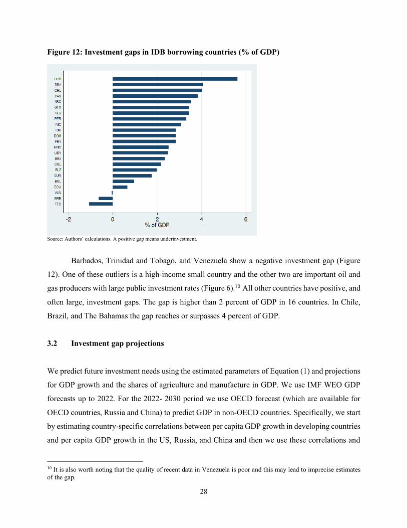
Figure 12: Investment gaps in IDB borrowing countries (% of GDP)

Source: Authors’ calculations. A positive gap means underinvestment.

Barbados, Trinidad and Tobago, and Venezuela show a negative investment gap (Figure

12). One of these outliers is a high-income small country and the other two are important oil and

gas producers with large public investment rates (Figure 6).10 All other countries have positive, and

often large, investment gaps. The gap is higher than 2 percent of GDP in 16 countries. In Chile,

Brazil, and The Bahamas the gap reaches or surpasses 4 percent of GDP.

3.2 Investment gap projections

We predict future investment needs using the estimated parameters of Equation (1) and projections

for GDP growth and the shares of agriculture and manufacture in GDP. We use IMF WEO GDP

forecasts up to 2022. For the 2022- 2030 period we use OECD forecast (which are available for

OECD countries, Russia and China) to predict GDP in non-OECD countries. Specifically, we start

by estimating country-specific correlations between per capita GDP growth in developing countries

and per capita GDP growth in the US, Russia, and China and then we use these correlations and

10 It is also worth noting that the quality of recent data in Venezuela is poor and this may lead to imprecise estimates of the gap.

29

OECD forecasts to predict GDP per capita in non-OECD countries. The shares of agriculture and

manufacturing in GDP are predicted using their 2010-2014 trend.

Table 12: Estimated Public Investment Demand 2022 Estimated demand Business as usual % GDP bill USD % GDP Gap (% GDP) Gap (bill USD)

EAP 6.3 1,472 13.2 -6.9 -1,613 ECA 7.3 461 2.9 4.4 278 LAC 7.7 578 3.6 4.1 308 MNA 8.5 227 6.4 2.1 56 SAS 7.2 352 5.4 1.8 88 SSA 7.9 201 4.4 3.5 89


Table 12 shows that by 2022 annual public investment demand in IDB borrowing countries

will increase from its current level of 6.7 percent of GDP (corresponding to $366 billion) to 7.7

percent of GDP (or $578 billion). This increase is mainly explained by structural transformation.

Projected increases in GDP per capita are likely to reduce public investment demand but, as the

economy moves away from agriculture and manufacturing into services, the demand for public

investment is projected to increase.

Assuming a business as usual scenario where public investment remains at its 2015 level

of 3.6 percent of GDP, the public investment gap projected in 2022 reaches 4.1 percent of GDP.

This implies that the annual public investment gap is expected to increase from an estimated $169

billion in 2015 (Table 11) to $308 billion by 2022. This large increase is driven by the 1-percentage

point increase in the estimated share in GDP of public investment demand, as well as the projected

increase in GDP by 2022.

Table 13: Public Investment Demand 2030 Estimated demand Business as usual % GDP bill USD % GDP Gap (% GDP) Gap (bill USD)

EAP 5.5 1,927 13.2 -7.7 -2699 ECA 7.4 814 2.9 4.5 495 LAC 8.0 911 3.6 4.4 501 MNA 8.2 333 6.4 1.8 73 SAS 7.2 532 5.4 1.8 133 SSA 8.2 328 4.4 3.8 152


30

Longer term estimates calculated using the same approach but with GDP per capita projections

obtained with the methodology explained above suggest that public investment demand in IDB

borrowing countries will reach 8 percent of GDP or $911 billion in 2030 (Table 13). With a

business as usual public investment scenario representing, as in 2015, an investment rate of 3.6

percent of GDP, the annual public investment gap reaches 4.4 percent of GDP in 2030 ($501

billion). This is almost three times larger than the current public investment gap of $169 billion.

4 Public Investment and the Sustainable Development Goals

So far, we estimated investment demand and investment gaps by using actual and projected data

on GDP growth and economic structure. However, we did not consider the possibility that countries

may try to reach certain targets as specified in the Sustainable Development Goals. In this section,

we propose a methodology that could be used to estimate the level of public investment necessary

for reaching some of the SDGs. We use the first target of the first SDG, which focuses on the

eradication of extreme poverty (i.e., people living with less than $1.25 PPP per day).11 We then

turn to two additional SDGs and compute the additional public investment gap to achieve the

reduction of child mortality under the age of 5 to 25 per thousand lives12 and the completion of

secondary school for all girls and boys.13 .

As first step, we estimate the impact of public investment on the poverty ratio. Table 14

shows that, controlling for country and year fixed effects, GDP per capita, and the agriculture and

manufacturing shares in GDP, public investment is negatively correlated with the poverty ratio.14

If we interpret these correlations as causal (which, of course, is a strong assumption), we can use

the estimates of Table 14 to back up the amount of investment necessary to reach a given poverty

target, while controlling for the projected increases in GDP per capita as well as changes in

agriculture and manufacturing shares.

11 With more data, the same approach could be applied to a larger number of indicators. 12 By 2030, end preventable deaths of newborns and children under 5 years of age, with all countries aiming to reduce under-5 mortality to at least as low as 25 per 1,000 live births 13 By 2030, ensure that all girls and boys complete free, equitable and quality secondary education leading to relevant and effective learning outcomes 14 GDP per capita is also negatively correlated with the poverty ratio, whereas the agriculture and manufacturing value-added shares in GDP do not seem to have a statistically significant impact on poverty rates.

31

Let us illustrate this procedure with an example. Consider the case of a country with a 9 percent

poverty rate (which is close to the average for LAC in the period 2010-2014). The first target of

the first SDG is: “By 2030, eradicate extreme poverty for all people everywhere, currently

measured as people living on less than $1.25 a day.” The estimates of Table 14 show that,

controlling for GDP per capita, a 1 percentage point increase in the ratio of public investment-to-

GDP is associated with a decrease in

poverty of 0.8 percentage points. They also

show that, controlling for the ratio of public

investment-to-GDP, a 1 percent increase in

GDP per capita leads to a 0.15 percentage

point reduction in poverty. Let us ignore the

changes in the shares of agriculture and

manufacturing value-added in GDP that are

statistically insignificant. Assuming the

country is projected to have an increase in GDP per capita of 50 percent by 2030, we can then

predict that this will reduce the poverty rate by 6 percentage points. To fully eradicate poverty, we

need a further reduction of 3 percentage points. This can be achieved with an increase in the ratio

of public investment-to-GDP of 2.4 percentage points (3*0.8=2.4). We can then add this 2.4

percentage point of additional public investment needed to eradicate poverty to the investment

demand projected in 2030 in Table 13. So, if the country in question had a public investment

demand of 8 percentage points, achieving this specific SDG would push the projected investment

demand in 2030 to 10.4 percent of GDP.

Table 15 provides the estimates of the public investment demand by region when we

include the public investment needs to reach the target of extreme poverty eradication to the

projected investment demand in 2030 reported in Table 13. Once we include the public investment

demand needed to reach the objective of eradicating extreme poverty, IDB borrowing members

will face a public investment demand that will increase from 8 percent of GDP projected in Table

13 to 8.2 percent of GDP ($934 billion). If public investment as a share of GDP remains at its 2015

level of 3.6 percent of GDP, then the public investment gap reaches 4.6 percent of GDP ($524

Table 14: Public investment and First SDG Dependent variable: poverty rate (%) Public Investment/GDP -0.818*** (-3.041) Ln(GDP per capita) -15.106*** (-5.635) Agriculture/GDP 0.134

(0.811) Manufacture/GDP -0.076

(-0.366) Country FE Y Year FE Y Observations 255

t-statistics in parentheses *** p<0.01, ** p<0.05, * p<0.1

32

billion). This is not much larger the 4.4 percent of GDP ($501 billion) projected for 2030 in Table

13, which did not include this specific SDG target.

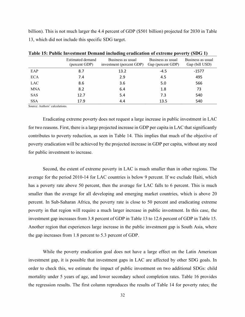
Table 15: Public Investment Demand including eradication of extreme poverty (SDG 1)

Estimated demand (percent GDP)

Business as usual investment (percent GDP)

Business as usual Gap (percent GDP)

Business as usual Gap (bill USD)

EAP 8.7 13.2 -4.5 -1577 ECA 7.4 2.9 4.5 495 LAC 8.6 3.6 5.0 566 MNA 8.2 6.4 1.8 73 SAS 12.7 5.4 7.3 540 SSA 17.9 4.4 13.5 540


Eradicating extreme poverty does not request a large increase in public investment in LAC

for two reasons. First, there is a large projected increase in GDP per capita in LAC that significantly

contributes to poverty reduction, as seen in Table 14. This implies that much of the objective of

poverty eradication will be achieved by the projected increase in GDP per capita, without any need

for public investment to increase.

Second, the extent of extreme poverty in LAC is much smaller than in other regions. The

average for the period 2010-14 for LAC countries is below 9 percent. If we exclude Haiti, which

has a poverty rate above 50 percent, then the average for LAC falls to 6 percent. This is much

smaller than the average for all developing and emerging market countries, which is above 20

percent. In Sub-Saharan Africa, the poverty rate is close to 50 percent and eradicating extreme

poverty in that region will require a much larger increase in public investment. In this case, the

investment gap increases from 3.8 percent of GDP in Table 13 to 12.6 percent of GDP in Table 15.

Another region that experiences large increase in the public investment gap is South Asia, where

the gap increases from 1.8 percent to 5.3 percent of GDP.

While the poverty eradication goal does not have a large effect on the Latin American

investment gap, it is possible that investment gaps in LAC are affected by other SDG goals. In

order to check this, we estimate the impact of public investment on two additional SDGs: child

mortality under 5 years of age, and lower secondary school completion rates. Table 16 provides

the regression results. The first column reproduces the results of Table 14 for poverty rates; the

33

second column provides results for mortality rates, and the third column for lower secondary school

completion rates.

Table 16: Public Investment and SDGs

Dependent variables:

(1) (2) (3)

Poverty Rate, % Mortality Rate, % Education Completion Rate

(Lower Secondary) Public Investment/GDP -31.563** -1.771*** 0.436** (-2.514) (-5.239) (2.056) Ln(GDP per capita) -18.788*** -24.570*** 16.896***

(-4.290) (-5.664) (5.783) Agriculture/GDP 0.134 1.181*** -0.252

(0.811) (4.778) (-1.519) Manufacture/GDP -0.076 0.963*** -0.586*** (-0.366) (2.956) (-2.794) Country FE Y Y Y Year FE Y Y Y Observations 255 468 382 R-squared 0.394 0.396 0.340 Number of id 103 124 121

t-statistics in parentheses *** p<0.01, ** p<0.05, * p<0.1

As expected increases in the ratio of public investment over GDP is correlated with

reductions in the mortality rate and increases in lower secondary education completion rates. A 1

percent increase in public investment leads to 0.18 percentage point reduction in the mortality rate,

and a 0.4 increase in the lower secondary completion rate.

In order to compute the additional public investment gap needed to achieve these two

additional goals, we calculate the investment need to reach each of the goals (poverty, mortality

under 5, and completion of lower secondary school) by 2030 as before, and then take the maximum

investment need. If public investment as a share of GDP remains at its 2015 level of 3.6 percent

of GDP in LAC, then achieving all three targets would imply a public investment gap of 6.3 percent

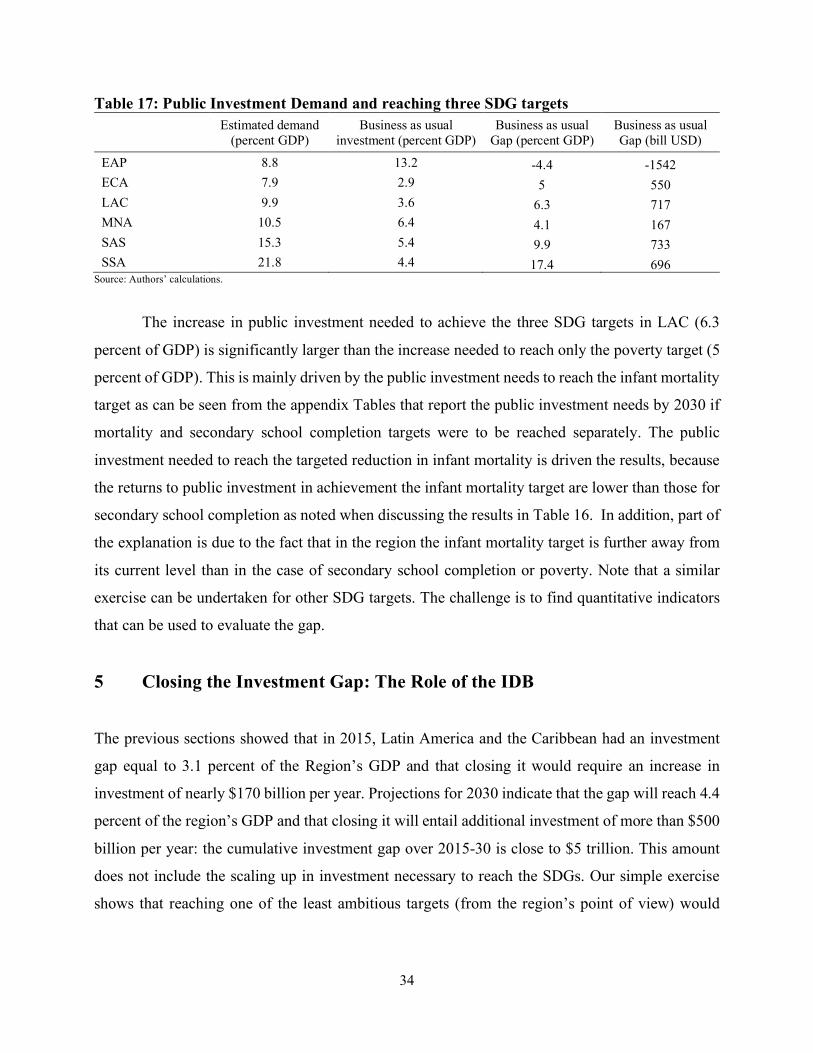
of GDP ($717 billion) (Table 17).

34

Table 17: Public Investment Demand and reaching three SDG targets Estimated demand

(percent GDP) Business as usual

investment (percent GDP) Business as usual

Gap (percent GDP) Business as usual Gap (bill USD)

EAP 8.8 13.2 -4.4 -1542 ECA 7.9 2.9 5 550 LAC 9.9 3.6 6.3 717 MNA 10.5 6.4 4.1 167 SAS 15.3 5.4 9.9 733 SSA 21.8 4.4 17.4 696


The increase in public investment needed to achieve the three SDG targets in LAC (6.3

percent of GDP) is significantly larger than the increase needed to reach only the poverty target (5

percent of GDP). This is mainly driven by the public investment needs to reach the infant mortality

target as can be seen from the appendix Tables that report the public investment needs by 2030 if

mortality and secondary school completion targets were to be reached separately. The public

investment needed to reach the targeted reduction in infant mortality is driven the results, because

the returns to public investment in achievement the infant mortality target are lower than those for

secondary school completion as noted when discussing the results in Table 16. In addition, part of

the explanation is due to the fact that in the region the infant mortality target is further away from

its current level than in the case of secondary school completion or poverty. Note that a similar

exercise can be undertaken for other SDG targets. The challenge is to find quantitative indicators

that can be used to evaluate the gap.

5 Closing the Investment Gap: The Role of the IDB The previous sections showed that in 2015, Latin America and the Caribbean had an investment

gap equal to 3.1 percent of the Region’s GDP and that closing it would require an increase in

investment of nearly $170 billion per year. Projections for 2030 indicate that the gap will reach 4.4

percent of the region’s GDP and that closing it will entail additional investment of more than $500

billion per year: the cumulative investment gap over 2015-30 is close to $5 trillion. This amount

does not include the scaling up in investment necessary to reach the SDGs. Our simple exercise

shows that reaching one of the least ambitious targets (from the region’s point of view) would

35

increase the 2030 gap by more than $20 billion and bring the cumulative gap over 2015-30 to $5.1

trillion.

To evaluate the effects the required scaling up of public investment on external and fiscal

sustainability, we conduct two simple exercises. First, we assume that countries have constant

saving rate and private investment. Given that the current account balance is equal to total savings

minus private and public investment, we estimate the current account implications of closing the

investment gap by subtracting the 2015 country-specific investment gap to the country’s current

account balance (we use the 2010-14 average).

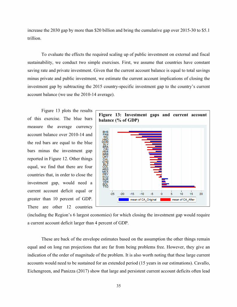
Figure 13 plots the results

of this exercise. The blue bars

measure the average currency

account balance over 2010-14 and

the red bars are equal to the blue

bars minus the investment gap

reported in Figure 12. Other things

equal, we find that there are four

countries that, in order to close the

investment gap, would need a

current account deficit equal or

greater than 10 percent of GDP.

There are other 12 countries

(including the Region’s 6 largest economies) for which closing the investment gap would require

a current account deficit larger than 4 percent of GDP.

These are back of the envelope estimates based on the assumption the other things remain

equal and on long run projections that are far from being problems free. However, they give an

indication of the order of magnitude of the problem. It is also worth noting that these large current

accounts would need to be sustained for an extended period (15 years in our estimations). Cavallo,

Eichengreen, and Panizza (2017) show that large and persistent current account deficits often lead

Figure 13: Investment gaps and current account balance (% of GDP)

36

to financial crises, high volatility, and sub-par economic growth. Hence, a systematic scaling up of

public investment will require an increase in the domestic saving rate (for a comprehensive

discussion of saving rates in Latin America and the Caribbean see Cavallo and Serebrisky, 2016).

We can examine the fiscal implications of closing the investment gap by conducting a

similar experiment. Specifically, we assume unchanged government revenues and current

expenditure and subtract from the observed fiscal balance the increase in public investment

necessary to close the public investment gap.

Figure 14 shows the results

of this exercise. The blue bars plot

the average fiscal balance over

2010-14 and the red bars are equal

to the blue bars minus the

investment gap reported in Figure

12. Other things equal, we find that

there are eight countries (including

Brazil, Argentina, Mexico, and

Colombia) that in order to close the

investment gap would need to have

a fiscal deficit greater than 6

percent of GDP and 4 other

countries where closing the investment gap would require a fiscal deficit larger than 4 percent of

GDP.

These back of the envelope estimates do not keep into account many factors (for instance,

the fact that public investment can have a positive effect on growth and fiscal revenues). However,

they illustrate that there are serious fiscal implications linked to closing the investment gap. All

large Latin American economies would need substantial fiscal deficits (going from 7.5 percent in

Brazil to 3 percent in Chile) sustained for a period of 15 years to close the investment gap.

Figure 14: Investment gaps and fiscal balance (% of GDP)

37

Scaling up public investment will require fiscal reforms but also public private partnership which

would allow the private sector to finance some investment projects that have been traditionally

financed with public funds.

The IDB can help countries in the region to close these gaps through lending and policy

advice. On the policy advice side, the Bank can help countries to design fiscal reforms aimed at

limiting the budgetary implications of scaling up public investment and creating an enabling

environment for prompting greater private sector

participation in infrastructure projects. The Bank can

also help countries to develop policies that can

promote domestic savings and therefore limit the

current account implications of scaling up public

investment (Cavallo and Serebrisky, 2016).

On the financing side, the question is the

impact of an increase in IDB lending on closing these

gaps. The horizontal bars in the top two panels of

Figure 15 plot the total public investment gap in 2014

for IDB borrowing countries and the red bars show

the share of the investment gap that could be covered

if IDB were to double its disbursements with respect

to the 2010-14 average. The top panel of the figure

shows that IDB disbursements are a small fraction of

the total investment gap of the 6 largest countries in

the Region (and these are gross disbursements, net

flows would paint an even bleaker picture).

There are, however, several small and medium sized

countries, plotted in the middle panel of Figure 15,

for which a scaling up of IDB lending could have a

significant effect in reducing the public investment gap. The bottom panel of Figure 15 shows that

Figure 15: IDB disbursements and investment gap (bill USD)

38

there are 9 countries for which IDB disbursements are close or greater than 20 of the public

investment gap. A scaling of IDB lending could have a substantial impact on public investment in

these countries.

There are two ways to interpret the data of the top panel of Figure 15. The first interpretation

is that the Bank cannot have any important effect in large countries and that it should concentrate

its lending on small countries. The second possible interpretation is that there is a large latent

demand for IDB lending. It is worth nothing that even in large countries, like Colombia and

Argentina, a doubling of IDB lending could reduce the public investment gap by nearly 8 percent.

Moreover, multilateral lending could contribute to closing the investment gap thanks to its catalytic

role for private sector financing.

One important question from IDB’s perspective is how its relative importance as a source

of funds for public investment in the

region has evolved across time. We

have therefore computed a time-

varying public investment gap by

considering not only the country

fixed effect (the time invariant gap),

but also the error term when

estimating equation (1). We then

compute the share of the public

investment gap in GDP, and the

share of IDB lending in the public

investment GAP and in GDP for

four sub-periods: 1995-1999, 2000-

2004, 2004-2009, 2010-2014. The results are reported in Figure 16. They suggest that while IDBs’

lending is relatively small with respect to the total public investment gap, since the turn of the

century its relative importance has been growing to reach 5.5 percent of the total public investment

gap in 2010-2014.

Figure 16: Investment gaps and IDB lending (% of GDP) over time

39

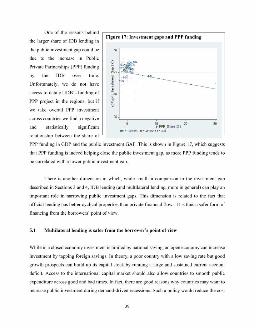
One of the reasons behind

the larger share of IDB lending in

the public investment gap could be

due to the increase in Public

Private Partnerships (PPP) funding

by the IDB over time.

Unfortunately, we do not have

access to data of IDB’s funding of

PPP project in the regions, but if

we take overall PPP investment

across countries we find a negative

and statistically significant

relationship between the share of

PPP funding in GDP and the public investment GAP. This is shown in Figure 17, which suggests

that PPP funding is indeed helping close the public investment gap, as more PPP funding tends to

be correlated with a lower public investment gap.

There is another dimension in which, while small in comparison to the investment gap

described in Sections 3 and 4, IDB lending (and multilateral lending, more in general) can play an

important role in narrowing public investment gaps. This dimension is related to the fact that

official lending has better cyclical properties than private financial flows. It is thus a safer form of

financing from the borrowers’ point of view.

5.1 Multilateral lending is safer from the borrower’s point of view

While in a closed economy investment is limited by national saving, an open economy can increase

investment by tapping foreign savings. In theory, a poor country with a low saving rate but good

growth prospects can build up its capital stock by running a large and sustained current account

deficit. Access to the international capital market should also allow countries to smooth public

expenditure across good and bad times. In fact, there are good reasons why countries may want to

increase public investment during demand-driven recessions. Such a policy would reduce the cost

Figure 17: Investment gaps and PPP funding

40

of building a country’s capital stock (factors of productions are cheaper during recessions) while

facilitating the recovery by providing a stimulus to domestic demand.

However, developing and emerging market countries have precarious access to

international finance and, as they tend to lose market access during recessions, they often

implement procyclical fiscal policies (Gavin and Perotti, 1997). Public investment is often the

adjustment variable and losing access to international financial flows can lead to budgetary cuts

which, besides deepening the recession in the short term, may also have long-term implications as

these cuts tend to concentrate on public investment (Easterly, Irwin, and Servén, 2008) and

infrastructure investment (Serebrisky et al., 2015).

Besides increasing the volatility of public investment, precarious access to international

financial markets may also reduce a country’s willingness to scale up investment by borrowing

abroad during good times when financing is available. This is because, with volatile access to

international finance, foreign borrowing is risky as highlighted by the economic literature on

original sin and sudden stops.

External debt is often denominated in foreign currency (Eichengreen, Hausmann, and

Panizza, 2007) and funding domestic investment projects that do not generate foreign earnings with

foreign currency debt can lead to dangerous currency mismatches. Another risk, highlighted by

the literature on sudden stops (Calvo, Izquierdo and Mejía, 2004, and Cavallo and Frankel, 2008),

is that countries that rely heavily on foreign savings tend to face sudden capital flight. These sudden

stops force the affected country to abruptly close its current account deficit. This outcome is usually

achieved through a combination of real exchange rate depreciation and import contraction, both of

which are typically accompanied by recessions, especially in the presence of foreign currency

debt.15

15 Because of these risks, which were at the center of the financial crises of the 1990s, many East Asia countries decided put in place policies aimed at reducing their net exposure to external debt. These policies consisted of either borrowing less or self-insuring by accumulating large foreign reserves, (Hausmann and Panizza, 2011). This was however an easy choice for East Asian countries characterized by high saving rates and no need to tap foreign markets to finance their sky-high investment rates. Things are more difficult for Latin American countries characterized by low saving rates.

41

While most multilateral lending is still denominated in foreign currency (hence, it does not

eliminate the risks linked to the presence of currency mismatches), lending by multilateral

development banks is either acyclical or countercyclical (Galindo and Panizza, 2017). It is thus

better suited for financing long-term investment projects, as it is not subject to sudden stops. It is

in this sense that lending by multilateral banks is a safer form of finance that can play an important

role for scaling up investment in emerging and developing countries. Cavallo, Eichengreen and

Panizza (2017) find that large current account deficits financed with official flows are less likely

to end with a financial crisis.

One puzzling element is that in good times, when liquidity is abundant, most Latin America

countries prefer to borrow from financial markets instead of borrowing from the multilaterals. The

standard explanation for this behavior is that when the spread between the interest rate changed by

official lenders and the rate charged by private lenders is low it is not worth to pay the higher costs

in terms of compliance linked to official lending. This way of reasoning seems myopic because it

does not keep into account the costs linked to the volatility of market finance.16 In future research,

it would be interesting to compare the total costs (interest rate + volatility) of market financing with

the total cost (interest rate + compliance) of official financing.

6 Conclusions This note provides a simple and transparent methodology for estimating public investment gaps in

developing countries together with a detailed analysis of these gaps in IDB borrowing countries.

We also develop a simple methodology for incorporating three SDG targets into our investment

gap estimates (poverty, infant mortality and lower secondary school completion).

We find that in 2015 the total public investment gap of IDB borrowers was close to $170

billion (3.1 percent of the Region’s GDP) and that the gap is expected to reach $501 billion (4.4

percent of the Region’s GDP) by 2030. If we were to add the necessary public investment needed

16 While it is true that when countries lose access to market finance, they can still get funding from the multilateral, the process is usually slow and emergency finance is often at a premium (in terms of both interest rates and conditionality) over regular lending facilities. Moreover, if multilaterals do not have enough demand in good times, their steady state balance sheet will remain small and hard to scale at time of crisis.

42

to reach the three SDGs examined, the public investment gap would reach $717 billion (6.3 percent

of the Region’s GDP) by 2030.

Most of the region’s largest economies have gaps well above 2 percent of GDP and Brazil

has a gap of 4 percent of GDP in 2015. Like all forecasting exercises, our estimates have a

substantial margin of errors and should be complemented with expert assessments of gaps in

specific areas.

Future research should focus on estimating confidence intervals for these predictions and

on building bounds that keep into account possible endogeneity problems with the methodology

described in this note. It would also be interesting to put the investment gaps on the left-hand-side

of a regressions analysis and study whether country characteristics are correlated with these gaps.

Potential control variables include private savings, the level of development, government balance,

current account balance, fiscal and monetary policy procyclicality, and the composition of public

debt. It would be also interesting to study the relationship between investment gaps and the

cyclicality of public investment spending. Finally, future research could expand our methodology

to alternative SDG targets.

43

References Afonso, António and Miguel St. Aubyn, 2016. Economic growth and public and private investment returns. Lisbon School of Economics and Management working paper 14. Abiad, Abdul, Davide Furceri, and Petia Topalova, 2016. The macroeconomics effects of public investment: Evidence from Advanced Economies. Journal of Macroeconomics 50, 226-240. Arellano, Manuel and Olympia Bover, 1995. Another Look at the Instrumental Variable Estimation of Error-Components Models, Journal of Econometrics 68, 29-51. Blundell, Richard and Stephen Bond, 1998. Initial Conditions and Moment Restrictions in Dynamic Panel Data Models. Journal of Econometrics 87, 115-143. Bourguignon, François, Carlos Diaz-Bonilla, Carlos, and Helmut Lofgren, 2008. Aid, Service Delivery, and the Millennium Development Goals in an Economy-wide Framework. The World Bank Development Economics Prospects Group. Policy Research Paper 4683. Washington,D.C.: World Bank. Calvo, Guillermo, Alejandro Izquierdo and Luis-Felipe Mejía. 2004. “On the Empirics of Sudden Stops: The Relevance of Balance-Sheet Effects.” Paper presented at the conference “Emerging Markets and Macroeconomic Volatility: Lessons from a Decade of Financial Debacles,” San Francisco, United States, Federal Reserve Bank of San Francisco, June 4-5. Cavallo, E., and J. Frankel. 2008. “Does Openness to Trade Make Countries More Vulnerable to External Crises, or Less? Using Gravity to Establish Causality.” Journal of International Money and Finance 27: 1430-1452. Cavallo, Eduardo, Barry Eichengreen, and Ugo Panizza (2017) Can countries rely on foreign saving for investment and economic development?, Review of World Economics. Cavallo, Eduardo and Tomás Serebrisky (2016) Saving for Development: How Latin America and the Caribbean Can Save More and Better, Palgrave McMillian. Dreger, Christian and Hans-Eggert Reimers, 2016. Does public investment stimulate private investment? Evidence for the Euro area. Economic Modelling 58, 154-158. Easterly, William, Timothy Irwin, and Luis Servén, 2008. "Walking up the Down Escalator: Public Investment and Fiscal Stability," World Bank Research Observer, vol. 23(1): pages 37-56. Eichengreen, Barry, Ricardo Hausmann, and Ugo Panizza, 2007., “Currency Mismatches, Debt Intolerance, and the Original Sin: Why They Are Not the Same and Why It Matters,” in Capital Controls and Capital Flows in Emerging Economies: Policies, Practices and Consequences, S. Edwards (ed.), National Bureau of Economic Research, Inc. and Chicago University Press, Chicago.

44

Fay, Marianne 2000. Financing the Future: Infrastructure Needs in Latin America, 2000-05." Policy Research Working Paper 2545. The World Bank, Washington DC. Fay, Marianne and Tito Yepes 2003. "Investing in infrastructure: what is needed from 2000 to 2010?"Policy Research Working Paper Series 3102, The World Bank. Galindo, Arturo and Ugo Panizza, 2017. "The Cyclicality of International Public Sector Borrowing in Developing Countries: Does the Lender Matter?" CEPR Discussion Papers 12243. Gavin, Michael and Roberto Perotti, 1997. “Fiscal Policy in Latin America,” in Bernanke and Rotenberg (eds.) NBER Macroeconomics Annual 1997, Volume 12: 11-72. Hausmann, Ricardo and Ugo Panizza, 2011. “Redemption or Abstinence? Original Sin, Currency Mismatches and Counter Cyclical Policies in the New Millennium,” Journal of Globalization and Development, 2(1) MDG Africa Steering Group 2008. Achieving the Millennium Development Goals in Africa: Recommendations of the MDG Africa Steering Group. Pritchett, Lant, 2000. The tyranny of concepts: CUDIE (Cumulated, depreciated, investment effort) is not capital. Journal of Economic Growth 5, 361-384. Ruiz-Nuñez, Fernanda and Zichao Wei, 2015. Infrastructure investment demands in emerging markets and developing economies. Policy Research Working Paper 7414, The World Bank, Washington, DC. Schmidt-Traub, Guido 2015 Investment Needs to Achieve the Sustainable Development Goals Understanding the Billions and Trillions* SDSN Working Paper. Paris and New York: Sustainable Development Solutions Network. Schmidt-Traub, Guido and Jeffrey Sachs. 2015. Financing for Sustainable Development: Implementing the SDGs through Effective Investment Strategies and Partnerships. SDSN Working Paper. Paris and New York: Sustainable Development Solutions Network. Serebrisky, Tomás, Ancor Suárez-Alemán, Diego Margot, Maria Cecilia Ramirez, 2015. Financing Infrastructure in Latin America and the Caribbean: How, How much and by Whom? Inter-American Development Bank.

45

Data Appendix

• Investment and capital stock data comes from the IMF Investment and Capital Stock

Dataset 2017. This dataset contains comprehensive and comparable data across countries

on public, private and total investment, as well as capital stocks for all IMF member

countries. These flows and stocks include public-private partnerships (PPPs) projects.

• Our key focus is on the public investment and the IMF dataset is comparable data across

170 countries (see Pritchett, 2000 for reasons why capital and investment flow data may

not be comparable across countries). Investment and capital stock data is computed using

PPP exchange rates to make them comparable across countries. This explains why the

investment numbers in the new IMF dataset are a bit larger than what one may be used to

observe for low-income countries.

• Data on infrastructure investment data is drawn from the Global Infrastructure Outlook

(GIO). The GIO contains infrastructure data for around 50 countries from 2007 until 2015.

• The infrastructure investment efficiency data is from the World Economic Forum and it

includes 170 countries from 2006 to 2014.

• GDP, GDP per capita, population, the share of agriculture value-added in GDP, and the

share of manufacturing value-added on GDP come from the World Bank’s World

Development Indicators 2017.

• GDP forecast data until 2022 is borrowed from the IMF’s World Economic Outlook (WEO)

and is available for 170 countries. For GDP forecasts after 2002, we use the OECD dataset,

which contains the GDP forecast for its member countries (including China and Russia)

until 2060.

• Data on poverty, child mortality under 5, and lower secondary enrollment corresponding to

SDG targets comes from World Development Indicators.

46

Appendix Tables

Appendix Table 1: Public Investment Demand including SDG infant mortality target

Region Estimated public investment demand

(% GDP)

Business as usual investment (% GDP)

Business as usual investment gap

(% GDP)

EAP 6.1 13.2 -7.1 ECA 7.9 2.9 5.0 LAC: IDB 9.9 3.6 6.3 MNA 10.5 6.4 4.1 SAS 15.3 5.4 9.9 SSA 21.5 4.4 17.1


Appendix Table 2: Public Investment Demand including SDG lower secondary education completion target

Region Estimated public investment demand

(% GDP)

Business as usual investment (% GDP)

Business as usual investment gap

(% GDP)

EAP 6.2 13.2 -7.0 ECA 7.9 2.9 5.0 LAC: IDB 8.6 3.6 5.0

MNA 8.7 6.4 2.3 SAS 8.1 5.4 2.7 SSA 9.3 4.4 4.9


investment gaps in idb borrowing...

Documents