Investment under Uncertainty, Debt and Taxes

current version, October 16, 2006

Andrea GambaDepartment of Economics, University of Verona

Verona, Italyemail:andrea.gamba@univr.it

Gordon A. SickHaskayne School of Business, University of Calgary

Calgary, Canadaemail: sick@ucalgary.ca

Carmen Aranda LeonUniversity of Navarra

Pamplona, Spainemail: sick@ucalgary.ca

Corresponding author:

Gordon A. SickHaskayne School of BusinessUniversity of CalgaryCalgary, AlbertaCanada T2N 1N4email: maranda@unav.es

Investment under Uncertainty, Debt and Taxes

Abstract

We present a capital budgeting valuation framework that takes into account bothpersonal and corporate taxation. We show broad circumstances under which taxes donot affect the martingale expectations operator. That is, the martingale operator isthe same before and after personal taxes, which we call “valuation neutrality”.

The appropriate discount rate for riskless equity-financed flows (martingale expec-tations or certainty-equivalents) is an equity rate that differs from the riskless debt rateby a tax wedge. This tax wedge factor is the after-tax retention rate for the corporatetax rate that corresponds to tax neutrality in the Miller equilibrium. We extend thisresult to the valuation of the interest tax shield for exogenous debt policy with defaultrisk. Interest tax shields accrue at a net rate corresponding to the difference betweenthe corporate tax rate that will be faced by the project and the Miller equilibriumtax rate. Depending on the financing system, interest tax shields can be incorporatedby using a tax-adjusted discount rate or by implementing an APV-like approach withadditive interest tax shields.

We also provide an illustrative real options application of our valuation approachto the case of an option to delay investment in a project, showing that the applicationof Black and Scholes formula may be incorrect in presence of personal and corporatetaxes.

Keywords: Investment under uncertainty, real options, capital structure, risk-neutralvaluation, corporate and personal taxation, default risk, interest tax shields, cost ofcapital, tax-adjusted discount rates.JEL classifications: G31, G32, C61

1

1 Introduction

Many models for valuing or optimizing capital investment decisions under uncertainty are

based on cash flows discounted at a risk-adjusted rate. However, the presence of leverage,

discretion and asymmetry forces a valuation approach based on computation of certainty-

equivalent, rather than expected, cash flows. This includes the real options approach.

The market maker who sets the relative prices of financial derivatives and their under-

lying instruments is typically taxed at the same rate on all financial instruments. Thus,

the common practice of discounting the certainty equivalent payoff of financial derivatives

(puts and calls on stocks, for example) at the riskless debt rate is appropriate. However,

we show that it is incorrect to carry this practice over to a real options setting because

the marginal investor of a capital investment project is likely to face a differential taxation

according to the type of instrument (i.e, equity or debt). In fact, the certainty equivalent

rate of return for equity funds is typically lower than that of debt funds.1

In addition, the interaction of personal and corporate taxes on various financing instru-

ments generates a net interest tax shield that may have positive or negative value. This

interaction is so often mishandled that few people recognize that it could just as likely have

a negative value as a positive value.

However, the following features commonly found in capital budgeting problems suggest

that the best valuation approach is to use certainty equivalent operators, tax-adjusted1The fact that a financial market maker does not use the same discount rate to value an investment as

a long-term capital investor would use does seem to lead to some arbitrage opportunities that we do notexplore. It may be difficult to take advantage of these arbitrage opportunities because a dynamic hedgebased on the long term capital value may generate adverse tax consequences, or may be hard to formbecause of incomplete markets.

On the other hand, it might be possible to synthesize the cash flows of a commodity producer, such asan oil company with very predictable reserves and production by a strip of forward or futures contractson oil and a strip of bonds. Both of these instruments are financial instruments and would be valued bydiscounting at the bond rate. They could be sold to an investor to replace an equity position in such afirm, and that investor may discount the flows at the riskless equity rate, which is less than the risklessdebt rate. This could represent a simple tax arbitrage.

2

discount rates for equity and a more sophisticated analysis of interest tax shields:

1. Projects are financed partially by equity and debt.

2. Personal and corporate taxes compound, and taxation of debt income differs from

that of equity income.

3. Some cash flows from a project, such as the tax advantage to debt are contingent on

the cash flows of the project and are lost in the event of default.

In this paper we first introduce a continuous-time valuation framework for cash flows

emerging in capital budgeting that takes into account personal and corporate taxes. We

show broad valuation neutrality circumstances under which taxes do not affect the equiv-

alent martingale measure.

Second, the paper shows how to adjust the value of asymmetric cash flows to com-

pute the value of debt and taxes under two different types of settings: default-free and

defaultable debt.

We can assume that debt is default-free if management constantly revises the debt level

of the firm to maintain a constant debt ratio.2 This assumption, first due to Miles and

Ezzel (1980, 1985), is popular in capital budgeting (e.g., Grinblatt and Liu (2002)), and is

considered as the benchmark case here. We find that the value of the interest tax shield can

be calculated either by an additive term that separates the value under different financing

scenarios (an adjusted present value or APV treatment), or by adjusting the discount

rate to reflect the tax wedge that separates the riskless market returns for instruments of2Stewart Myers has pointed out in private communication that if debt is continuously rebalanced to

keep a constant debt ratio, there can be no default on the debt. As the firm’s cash flows fall, its value falls,so the firm must repurchase debt and replace it with equity to keep the debt ratio constant. By the timethe firm approaches bankruptcy, there is no debt upon which to default.

In discrete time, there could be default even with a policy of rebalancing debt to keep a constant debtratio at the rebalance dates.

3

different tax classes in what we will call a tax-adjusted discount rate (TADR) approach.

Later, we assume that debt is defaultable and incorporate the effect of the probability of

default into the valuation.

The paper concludes by discussing an application of our results to a real options setting.

For clarity sake, we have selected the basic case of an option to delay an investment decision.

We demonstrate that the the project can be evaluated according to the Black, Scholes, and

Merton formula. However, using the riskless debt rate as the discount factor would be

a mistake, because the personal tax rate for bond investment income and that for stock

investment income are usually different.

The valuation of asymmetric cash flow is ubiquitous in corporate finance. To price

corporate securities, Merton (1974) sought to develop a theory for pricing bonds along

Black-Scholes lines with a significant probability of default. However, he did not include

taxes of any kind in his analysis, so the Black-Scholes setting was appropriate. Later

on, Brennan and Schwartz (1978), Leland (1994) and Leland and Toft (1996) became

aware of the importance of corporate income taxes and, accordingly, included corporate

taxation in their debt pricing and optimal capital structure models. Our work extends

this previous research by considering personal as well as corporate taxation. Kane et al.

(1984) did analyze the value of interest tax shields with personal taxes for risky debt where

the unlevered firm value could jump to zero according to a Poisson process. They did

not incorporate flexibility, so their valuation is a european option model of default. They

have a riskless rate for equity-financed flows that differs from the debt rate, but they find

that interest tax shields have a positive value. Our paper shows that interest tax shields

can have a negative or a positive value. More recently, Cooper and Nyborg (2004) model

tax- and risk-adjusted discount rates when the company follows the Miles-Ezzell leverage

policy but debt is risky, and both corporate and personal taxes are considered. Likewise,

4

Fernandez (2004, 2005), Fieten et al. (2005) and Cooper and Nyborg (2006) debate the

issue of whether or not the value of the debt tax saving is equal to the present value of tax

shields. They use a risk-adjusted discount rate settings, and a Miles-Ezzell leverage policy

while only considering corporate taxes. In contrast, we value general cash flows emerging

in capital budgeting using a certainty equivalent approach.

Our analysis goes beyond these papers in the following ways. It incorporates personal

and corporate taxes, a variety of debt policies and uses a certainty-equivalent approach to

risk. It discusses the appropriateness of various tax models. It also considers non-linear

cash flows that are not accurately valued with risk-adjusted discount rates, such as cash

flows with optionality, like real options, or asymmetric cash flows, like tax shields.

An outline of our work is as follows. In Sections 2 and Section 3, we provide an equi-

librium valuation approach in continuous-time for real and financial assets in an economy

with personal and corporate taxes, where tax rates on bonds and stocks are different. This

is the generalized Miller model. In Section 4 we present a continuous-time capital budget-

ing valuation approach for levered and unlevered real assets. Using continuous time allows

us to apply the results directly to such valuation problems (including real options), but the

results have natural interpretations in discrete time, as well. We start with the case of no

default risk, and then we consider defaultable debt with exogenous default. Debt policy

is taken as exogenous in the sense that it is not subject to optimization.3 In Section 5

we introduce the basic real option to delay an investment under the assumption that the

incremental debt to finance the real asset is issued conditional on the decision to invest.

The debt policy is still exogenous. Section 6 provides concluding remarks.3Footnotes 14 and 17 discuss how our approach can be extended to endogenous optimization of capital

structure and default decisions.

5

2 Asset valuation in a generalized Miller economy

2.1 Tax equilibrium

We assume a continuous-time Miller (1977) economy that is generalized to allow for cross-

sectional variation in corporate tax rates. In general, the personal tax rate for bond

investment income is different from the personal tax rate for stock investment income.

Miller assumes that there is cross-sectional variation in personal tax rates, but not corporate

tax rates. Thus, in his tax equilibrium, all corporations are indifferent about capital

structure, but investors have a tax-induced preference for debt or equity, leading to tax

clienteles. By allowing cross-sectional variation in corporate tax rates, as in Sick (1990),

only firms at the margin are indifferent (on a tax basis) between issuing debt and equity, and

firms with a marginal tax rate τ c below the marginal firm’s rate rate (τ c − τm = τ? < 0)

prefer to issue equity and firms with a tax rate above the marginal firm’s rate of the

marginal firm (τ? > 0) prefer to issue debt.

We assume that capital gains and coupons in bond markets are taxed at the same rate

τ b, and capital gains and dividends in equity markets are taxed at the same rate τ e, for the

marginal investor. The operators for investor or personal tax are assumed to be linear at

any date t, in the sense that income and losses from a particular investment are taxed, or

generate tax relief, at the same rate.4 On the other hand, the tax scheme for corporations

need not be linear. We allow τ c, τ b and τ e to be F-adapted stochastic processes, i.e. they

are determined as a function of the (stochastic) factors underlying the economy, but they4In general, individual investors do have a progressive tax structure, with increasing rates at increasing

levels of income. What we are assuming here is that a particular investment that the investor is pricingdoes not have income variations so large that it moves the investor to higher or lower tax brackets. Thekey assumption for this paper is that the marginal investment gains and losses (at the investor level) for aparticular asset are taxed at the same rate and that there is no kink in the tax curve as an asset goes froma gain to a loss.

Note, also, that we are speaking of the marginal tax rates of the marginal investor or firm, and assumethe reader can distinguish which “marginal” to use in any particular context.

6

must have continuous sample paths, almost surely. In general, τ b and τ e are different.

Ross (1987) established the existence of equilibrium and of an EMM for an economy with

personal taxes and a convex tax schedule. These assumptions are satisfied in our setting.

Consider a firm with tax rate τ c that is deciding whether to issue debt or equity to an

investor with tax rates τ e and τ b on equity and debt, respectively. If

(1− τ b) < (1− τ c)(1− τ e), (2.1)

then the firm has the ability and incentives to issue equity on terms that would be more

favourable to the marginal investor than debt a issue. To see this, suppose riskless debt

has a yield of rf . Then, if equation (2.1) holds, it is possible to choose a rate of return rz

for equity,5 so that the after-corporate-tax cost of equity paid by the company is less than

that of debt cost and, simultaneously, the after-all-tax rate of return for equity received by

the investor is higher than that of debt. That is, we can choose any value of rz such that

1− τ b

1− τ erf < rz < (1− τ c)rf .

On the one hand, this implies that (1−τ b)rf < (1−τ e)rz, so that the investor achieves

a higher after-all-tax return on equity than debt. On the other hand, it implies that

rz < (1 − τ c)rf , so that the cost of equity to the firm is lower than the after-tax cost of

debt. Thus, if (2.1) cannot hold for the marginal investor and the marginal firm with an

equilibrium economy, since the firm and the investor can both be better off by switching

some debt to equity.

Similarly, the marginal firm has incentives to issue (and the marginal investor has an5We set aside the risk premium for a moment, so that rz is a riskless yield. We will address this point

later on.

7

incentive to buy) debt rather than equity if

(1− τ b) > (1− τ c)(1− τ e) .

In equilibrium, there will be no further incentives for the firm to issue debt to retire

equity, or to issue equity to refund debt. Denoting the marginal firm’s tax rate by τm,

we have the Miller (1977) equilibrium relationship amongst the marginal tax rates of the

marginal investor and marginal firm:

(1− τ b) = (1− τm)(1− τ e) .

Thus, we have established the following proposition:

Proposition 1. If the marginal firm has tax rate τm, and the marginal investor has mar-

ginal tax rates τ e in equity and τ b on debt, then:

1− τm =1− τ b

1− τ e. (2.2)

Moreover, the market yields on riskless debt and equity are related by the following tax

wedge:

rz = (1− τm)rf . (2.3)

Thus, it is appropriate to refer to rz as a tax-adjusted discount rate. Equation (2.3)

provides a way to estimate the marginal tax rate τm, since rz and rf can either be observed

or derived from security prices.

The equilibrium rates of return on the money market and stock market are the same

after all taxes for the marginal investor. Defining this common after-all-tax return to be

8

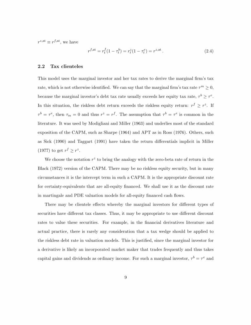
rz,at ≡ rf,at, we have

rf,at = rft (1− τ b

t ) = rzt (1− τ e

t ) = rz,at . (2.4)

2.2 Tax clienteles

This model uses the marginal investor and her tax rates to derive the marginal firm’s tax

rate, which is not otherwise identified. We can say that the marginal firm’s tax rate τm ≥ 0,

because the marginal investor’s debt tax rate usually exceeds her equity tax rate, τ b ≥ τ e.

In this situation, the riskless debt return exceeds the riskless equity return: rf ≥ rz. If

τ b = τ e, then τm = 0 and thus rz = rf . The assumption that τ b = τ e is common in the

literature. It was used by Modigliani and Miller (1963) and underlies most of the standard

exposition of the CAPM, such as Sharpe (1964) and APT as in Ross (1976). Others, such

as Sick (1990) and Taggart (1991) have taken the return differentials implicit in Miller

(1977) to get rf ≥ rz.

We choose the notation rz to bring the analogy with the zero-beta rate of return in the

Black (1972) version of the CAPM. There may be no riskless equity security, but in many

circumstances it is the intercept term in such a CAPM. It is the appropriate discount rate

for certainty-equivalents that are all-equity financed. We shall use it as the discount rate

in martingale and PDE valuation models for all-equity financed cash flows.

There may be clientele effects whereby the marginal investors for different types of

securities have different tax classes. Thus, it may be appropriate to use different discount

rates to value these securities. For example, in the financial derivatives literature and

actual practice, there is rarely any consideration that a tax wedge should be applied to

the riskless debt rate in valuation models. This is justified, since the marginal investor for

a derivative is likely an incorporated market maker that trades frequently and thus takes

capital gains and dividends as ordinary income. For such a marginal investor, τ b = τ e and

9

hence rz = rf even if they finance their positions entirely with equity.

On the other hand, for real assets, the marginal investor is likely a taxable individual

who holds shares in a corporation. If the real option is entirely financed with equity, then

it is appropriate to use a riskless rate rz < rf .

In what follows, we only require that all tax rates be between 0 and 1: 0 ≤ τ b, τ e, τ c, τm <

1.

Tax arbitrage has a tendency to make all firms behave as if they have the same tax

rate. At the corporate level, an arbitrage scheme could involve a highly taxed firm, with

τ c > τm or (1− τ b) > (1− τ c)(1− τ e), issuing debt to acquire its own equity, for example.

Or, it could involve a low-tax firm, with τ c < τm, issuing equity to buy back debt. We

assume that there are tax laws and agency costs6 that prevent a firm from undertaking

such an arbitrage transaction. Thus, there will generally be firms with τ? > 0 and firms

with τ? < 0 in this generalized Miller tax equilibrium.

It is more difficult to generate tax arbitrage opportunities that would have all investors

facing the same effective personal tax rate as that held by the marginal investor. This is

because personal tax laws identify the individual and generally change when a financial

entity (such as a corporation, mutual fund or trust) is inserted between the investor and

the investment vehicle. There will generally be investors who prefer debt to equity and

investors who prefer equity to debt in this generalized Miller tax equilibrium. Indeed,

Miller (1977) also assumed this. For example, suppose an investor pays little or no tax on

any investment (e.g. a pension fund), but the marginal investor pays higher tax on debt

than on equity. The untaxed investor would prefer the tax benefits of debt, but this will

prevent the investor from earning risk premia paid on equity investments. We assume that

any attempt to convert an equity investment with a risk premium to a debt instrument for6See for instance, Myers and Majluf (1984).

10

tax purposes is prevented by tax law.

3 Stochastic model

We assume an economy with complete financial markets that has personal and corporate

taxes. The time horizon is T , the underlying complete probability space is (Ω,F , P), where

the set of possible realizations of the economy is Ω, the σ-field of distinguishable events at T

is F , and the actual probability on F is P. We denote by F = Ft, t ∈ [0, T ] the augmented

filtration or information generated by the process of security prices, with FT = F .

3.1 Stochastic tax rates

Under many tax systems, such as the US tax code, the tax benefit of a bond coupon

payment is fully allowed only if the firm’s EBIT is greater than the coupon. If it is less, a

tax loss occurs that can be carried forward or backwards against positive taxable income.

If it is carried forward, the effective marginal tax rate is reduced by a loss of time value

of money, as observed by Leland (1994, p. 1220). We assume that the uncertainty in the

effective tax rate is caused by other cash flows of the firm that are independent of the

project’s tax rate. This allows us to model the carryforwards with a stochastic tax rate τ c.

Because the tax rate is independent of the project under consideration, all of our proofs

can be done conditional on the value of τ c, and then an expectation take over this risk. It

is quite likely that many of the valuation results can be extended to the situation where

tax rates are not independent of project cash flows.

We consider a firm that may have many projects that are independently financed with

non-recourse or project financing. Thus, default and bankruptcy events are confined to

each project and don’t affect the rest of the firm. The shocks to earnings of projects can

affect the tax rate faced by other projects. We assume that these shocks to the tax rate

11

τ c are independent of the shocks to the cash flows to the project we analyze. This would

happen for an arbitrarily small project or for one where the corporate tax rate is constant.

Similarly, we can have the marginal firm’s tax rate τm to be stochastic, but we assume

it to be independent of the project cash flows. The stochastic nature of tax rates is not

essential to achieve the results of this paper and readers may find it more convenient to

think of the tax rates as being deterministic or even constant.

Taxes introduce a risk-sharing mechanism between government and taxed investors.

This could cause a difference between the equilibrium EMM pricing measure with and

without personal taxes. Or, the EMM could differ for different tax clienteles. We will

establish a valuation neutrality principle, which says that the equilibrium pricing measure

is unchanged by the presence of taxation. For valuation purposes, this means that the

expectation (under the EMM) of the pre-tax cash flow stream of a security, discounted at

a pre-tax rate, is equal to the expectation (under the same EMM) of the after-tax cash

flow stream, discounted at an after-tax rate.

A second important issue introduced by taxation of security returns is the presence of

timing options related to taxation of capital gains, as pointed out by Constantinides (1983).

Taxation of capital gains produces timing options due to a (rational) delay of liquidation

of positions in financial securities, until a date of forced liquidation, if the accrued capital

gain is positive and the anticipation of liquidation of the position if the capital gain is

negative, to take advantage of the tax credit.

We avoid these timing options by assuming that capital gains are taxed as accrued,

as if the investor were to have a mark-to-market cash flow that induces the capital gain.

Taxation of accrued capital gains is one example of a holding-period neutral tax scheme in

which the tax scheme does not introduce any timing options related to taxation of capital

gains. Auerbach (1991), Auerbach and Bradford (2001) and Jensen (2003) describe taxa-

12

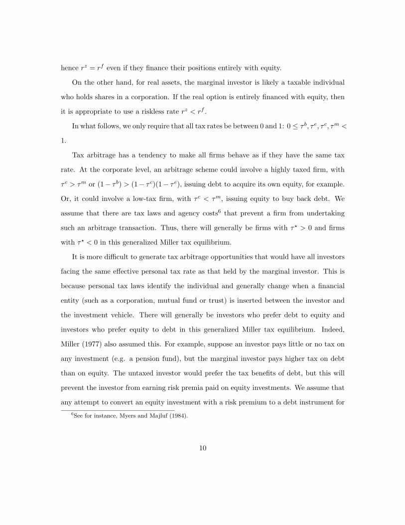
tion schemes that provide holding-period neutrality. It may be that our results generalize

to these other tax schemes as well, but that is a topic for future research.

3.2 EBIT and asset-price dynamics

Suppose the process for EBIT, under the actual probability measure is

dXt = g(Xt, t)dt + σ(Xt, t)dZt . (3.1)

Consider a project of value V = V (Xt, t) that pays equity holders the after-corporate-

tax cash flow at the rate

Y (Xt, τct , t), 0 ≤ t ≤ θp, (3.2)

where the project life is θp ≤ ∞. For an unlevered firm, Y (Xt, τct , t) = Xt(1 − τ c

t ). For a

levered firm, we will break out interest payments and interest tax shields by having a more

general form for Y in equation (4.2).

Since the EBIT process is not traded, we will value the claim to the equity-financed

stream Y by using an after-all-tax version of the consumption CAPM, as developed in

Constantinides (1983, Theorem 6) and used by others, such as Kane et al. (1984). Ross

(2005) also uses a general equilibrium after-all-tax model to get the market price of risk.7

Then we will calculate a sum of values of individual cash flows, as in Constantinides (1978).

To keep the notation convenient, suppose the market risk premium for the diffusion dZ is

λ in an after-tax consumption CAPM.8

7We would get the same results with replication arguments using a traded security. Interestingly, thehedge ratios used for the replication do not need a tax adjustment.

8That is, suppose a security has price P following

dP = µ(P )dt + σ(P )dZ

and pays a dividend at the rate Pδ(P ). Then, by the after-tax consumption CAPM, we have the instanta-

13

By Ito’s lemma, the after-all-tax wealth gain to the equity investor follows the process

(σ2(X, t)

2∂2V

∂X2+ g(X, t)

∂V

∂X+

∂V

∂t+ Y (X, τ c

t , t))

(1− τ e)dt

+ σ(X, t)∂V

∂X(1− τ e)dZt .

Here we take advantage of the fact that the capital gains are taxed as accrued to the

investor and at the same rate as the dividend distribution Y .

Taking expectations under the actual probability measure P, the expected after-all-tax

growth rate in wealth from the investment is

(σ2(X, t)

2∂2V

∂X2+ g(X, t)

∂V

∂X+

∂V

∂t+ Y (X, τ c

t , t))

(1− τ e) . (3.3)

In the after-tax consumption CAPM equilibrium, this must equal the riskless rate after

tax plus the risk premium

(1− τ e)(

rz + λ∂V

∂X

σ(X, t)V

)V . (3.4)

Equating (3.3) and (3.4) and simplifying yields the following proposition:

Proposition 2. Under the assumptions of this section, including personal taxation, the

neous required rate of return:„µ(P )

P+ δ(P )

«(1− τe) = rz(1− τe) + λ

σ(P )

P(1− τe) .

Since dividends and capital gains are taxed at the same rate in our model, the factor (1 − τe) factors outand this becomes the same as a pretax consumption CAPM:

µ(P )

P+ δ(P ) = rz + λ

σ(P )

P.

14

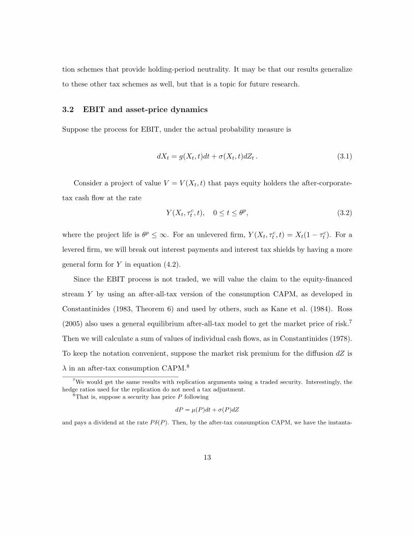
value of an equity-financed real asset satisfies the fundamental after-all-tax PDE:

(12σ2(X, t)

∂2V

∂X2+ g(X, t)

∂V

∂X+

∂V

∂t

)(1− τ e)

+ Y (Xt, τct , t)(1− τ e) = rz,atV (3.5)

where the risk-neutral growth rate is

g(X, t) ≡ g(X, t)− λσ(X, t) , (3.6)

whenever 0 ≤ t ≤ θp.

We also have the equivalent pretax PDE:

12σ2(X, t)

∂2V

∂X2+ g(X, t)

∂V

∂X+

∂V

∂t+ Y (Xt, τ

ct , t) = rzV , (3.7)

where the risk-neutral growth rate g is the same as defined in (3.6).

Proposition 3. If the assumptions of Proposition 2 hold and the project has residual

terminal value at time θp of

Vθp = V (Xθp , θp) = TV(Xθp , θp) , (3.8)

then

V (Xt, t) = Bzt Et

[∫ θp

t

Y (Xs, s)Bz

s

ds +TV(Xθp , θp)

Bzθp

](3.9)

15

where the money market account for riskless equity is

Bzu = exp

(∫ u

0rzsds

). (3.10)

Proof. Since the capital gains on changes in V are taxed as accrued, there is no personal

tax on the final distribution of TV(Xθp , θp) to the investor. We can use the Feynman-Kac

solution9 to the PDE (3.7) to obtain the result.

Characterizing the value as the expectation of a discounted stream of payoffs is very

useful, because it allows us to value projects by Monte Carlo simulation, even if they are

american real options where the manager can adjust strategies in response to the arrival

of information.

3.3 Valuation neutrality

Note that the risk-neutral growth rate g and hence the risk-neutral expectation operator

E is the same for the pre-personal-tax and after-all-tax valuation models. This means that

taxation affects the valuation only through the cashflow process and the discount rate, but

it does not affect the risk premium or certainty-equivalent calculation.10

We refer to this principle as valuation neutrality.9See, for example, Duffie (2001, pp. 340–346).

10Ross (1987) shows that there is a martingale pricing operator in the presence of taxes. His resultsare general and, in our setting, establish a risk-neutral expectation operator (or, equivalently, a certainty-equivalent operator) after all taxes, as well as risk-neutral expectation operators for debt flows beforepersonal tax and for equity flows before personal tax. There is no immediate guarantee that these pricingoperators are related or equivalent. Sick (1990) raised this question in a discrete-time setting and showedthat the certainty equivalent operators associated with these pricing operators are all identical to eachother. That is, taxes and tax shields do not generate a risk premium. Proposition 2 extends this result tocontinuous time.

16

3.4 After-all-tax valuation

The mark-to-market taxation of capital gains results in a cash-flow stream that is similar

to a dividend stream, and this has to be considered if we want to compute values from

after-all-tax cash flows.

Proposition 4. Under the assumptions of Propositions 2 and 3, the value of the real asset

satisfies the following expectation:

Vt = Bz,att Et

[∫ θp

t

(1− τ eu)Y (Xu, u)Bz,at

u

du−∫ θp

t

τ eu

Bz,atu

dVu +Vθp

Bz,atθp

], (3.11)

where the after-tax money market account for riskless equity is

Bz,atu = exp

(∫ u

0rz,ats ds

). (3.12)

Proof. The proof is an extension of the proof of the Feynman-Kac result, as discussed, for

example in Duffie (1988, Section 21). We will show that the solution to the martingale

valuation (3.11), will also satisfy the fundamental valuation PDE (3.7). Then we appeal

to the uniqueness of the solution of the PDE subject to the terminal condition (3.8).

Define the differential operator D such that if a real-valued function f ∈ C2,1, then

Df(x, t) =12σ2(x, t)

∂2f(x, t)∂x2

+ g(x, t)∂f(x, t)

∂x+

∂f(x, t)∂t

. (3.13)

where 0 ≤ t ≤ θp. Define the after-all-tax discounted value of V as

W (x, θ) ≡ V (x, θ)Bz,at

θ

, (3.14)

17

for t ≤ θ ≤ θp. By equation (3.11),

W (Xt, t) = Et

[∫ θ

t

(1− τ eu)Y (Xu, u)Bz,at

u

du−∫ θ

t

τ eu

Bz,atu

dVu +Vθ

Bz,atθ

]

= Et

[∫ θ

t

(1− τ eu)Y (Xu, u)Bz,at

u

du−∫ θ

t

τ eu

Bz,atu

dVu

]+ Et [W (Xθ, θ)] . (3.15)

Thus

Et [W (Xθ, θ)]−W (Xt, t) = −Et

[∫ θ

t

(1− τ eu)Y (Xu, u)Bz,at

u

du−∫ θ

t

τ eu

Bz,atu

dVu

]= −Et

[∫ θ

t

(1− τ eu)Y (Xu, u)Bz,at

u

du−∫ θ

t

τ eu

Bz,atu

DV du

](3.16)

The second equality comes from evaluating dVu by Ito’s lemma and noting that the diffusion

term has an expectation of zero.

Applying Ito’s formula to W gives

W (Xθ, θ)−W (Xt, t) =∫ θ

tDWdu +

∫ θ

t

∂W

∂xσ(xu)dZu . (3.17)

Taking risk-neutral expectations, the second term on the right also becomes zero. The left

side is the same as the left side of equation (3.16), so we can equate the right sides, getting:

Et

[∫ θ

t

(DW +

(1− τ eu)Y (Xu, u)Bz,at

u

− τ eu

Bz,atu

DV

)du

]= 0 .

This holds for all θ ∈ [t, θp], including values arbitrarily close to t, and this can only happen

if the integrand is identically zero. Thus

DW +(1− τ e

t )Y (Xt, t)Bz,at

t

− τ et

Bz,att

DV = 0 . (3.18)

18

Now, we can evaluate DW by substituting the definition (3.14) for W , expanding the

differential operator and applying the product rule and chain rule:

DW =12σ2(x, t)

∂2W

∂x2+ g(x, t)

∂W

∂x+

∂W

∂t

=σ2(x, t)2Bz,at

t

∂2V

∂x2+

g(x, t)Bz,at

t

∂V

∂x+

1Bz,at

t

∂V

∂t− rz

t (1− τ e)Bz,att(

Bz,att

)2 V

=1

Bz,att

DV − rzt (1− τ e)Bz,at

t

V .

Substituting for DW in equation (3.18) and simplifying gives equation (3.7), which is the

desired result.

The second term in the expectation of the martingale valuation (3.11) is the present

value of the mark-to-market capital gains taxation where the initial capital gains basis is

Vt.11 If we take the same initial basis, but assume that capital gains are only taxed when

realized, then we have the following variant of the valuation (3.11), which is constructive:

Vt = Bz,att Et

[∫ θp

t

(1− τ eu)Y (Xu, u)Bz,at

u

du +(1− τ e

T )Vθp + τ eT Vt

Bz,atθp

].

In this case, there is no simple pre-personal-tax equivalent valuation comparable to equa-

tion (3.9).

4 Valuation of levered and unlevered projects

We consider a project with life θp ≤ ∞ and EBIT following (3.1). We assume there is no

residual value at the end of the project, so TV(Xθp , θp) = 0.11It may be more natural to take the basis to be V0, since we allow t to vary. This just adds another

term to (3.11) for the valuation of the capital gains from 0 to t, and we omit it for brevity.

19

4.1 Valuation of an unlevered project

For this section, suppose Y (Xt, τct , t) = Xt(1− τ c

t ) is the unlevered earnings before interest

but after corporate tax. The risk-neutral drift g(X, t) is given in (3.6). The value of the

unlevered project U(x, t) is given by Proposition 3:

U(x, t) = Bzt Et

[∫ θp

t

Xs(1− τ cs )

Bzs

ds

](4.1)

for 0 ≤ t ≤ θp.

4.2 Valuation of a levered project

The sum of the values of the debt and equity claims against a project is called its Adjusted

Present Value or APV. Suppose the firm is financed with debt paying a coupon at the rate

Rt = R(Xt, t). This can be a fixed coupon, or a growing or amortizing coupon. It can also

be a risky coupon, where payments are a function of EBIT, X. We could have the coupon

depend on another random variable, but for simplicity, we keep the dimensionality of the

risk to one. The debt matures at time θd ≤ θp with a promised principal repayment of P

to the bondholders.

For t ≤ θd, the cash flow to equity-holders is at the rate (Xt − Rt)(1 − τ ct )(1 − τ e

t )

and that to debt-holders is at the rate Rt(1− τ bt ). After the debt is retired, the project is

financed completely with equity and we can keep the same representation of cash flow to

equity holders by setting Rt = 0 for θd < t ≤ θp. Thus, the total after-all-tax cash flow

from the project to the equity and debt investors is (dropping the common subscript t):

X(1− τ c)(1− τ e) + R(1− τ b) = (X(1− τ c) + τ∗R) (1− τ e) (4.2)

≡ Y (X, τ c)(1− τ e) ,

20

for 0 ≤ t ≤ θd, where the net rate of interest tax shield benefits is τ? = τ c − τm and τm is

the marginal tax rate defined in (2.2). This formula has the following important features:

1. The term τ∗R is the interest tax shield.

2. The factor (1 − τ e) emerges on the right side of the first equality. In effect, the tax

shield accrues to equity investors and is taxed at their marginal rate.12

3. We can define the “after-corporate-tax levered cash flow” Y = X(1 − τ c) + τ∗R by

the last equality, since the factor (1− τ e) is common in the second equality.

Note that τ? = τ c − τm is the rate at which net tax shields accrue to investors. The

traditional literature is based on interest tax shields having positive value, which requires

τ? > 0. However, since τ? is based on the difference between the firm’s tax rate τ c and the

marginal firm’s tax rate τm, interest tax shields could just as easily have negative value

as they have positive value. For high-tax firms, they have positive value, and for low-tax

firms, they have negative value.

Since we have an after-all-tax cash flow that is taxed at the personal equity rate, we

can apply Proposition 3 to obtain the following valuation result:

Proposition 5. The APV, incorporating the value of the tax shield, satisfies the funda-

mental PDE:

12σ2(X, t)

∂2V

∂X2+ g(X, t)

∂V

∂X+

∂V

∂t+ Xt(1− τ c

t ) + τ∗t Rt = rzt V. (4.3)

12Sick (1990) was the first to point out this fact, but it has been observed by others, such as Ross (2005).One interpretation of (4.2) is the following: the interest tax shield can be interpreted as a swap of debt forequity. The swap is valued by the marginal investor, who is indifferent between receiving cash flow fromequities and cash flows from bonds. At t = 0, the firm swaps B dollars of riskless or zero-beta equity claimsfor an equivalent amount (at the market value) of debt, so, the initial net change in investment for investorsis equal to 0. At every coupon date, the firm avoids having to remit the required rate of return rzB to equityholders, but must pay rf (1− τ c)B to debt-holders. The net gain for equity-holders is rzB − rf (1− τ c)B,which can be rewritten using the generalized Miller equilibrium (2.3) as rfB(τ c − τm).

21

with boundary conditions V (θd, Xθd) = U(θd, Xθd) and U(θp, Xθp) = 0, and is

V (x, t) = Bzt Et

[∫ θd

t

Xs(1− τ cs ) + τ∗s Rs

Bzs

ds +U(θd, Xθd)

Bzθd

]

= U(x, t) + Bzt Et

[∫ θd

t

τ∗s Rs

Bzs

ds

], (4.4)

for 0 ≤ t ≤ θd. The second term in the right side is the value of the stream of interest tax

shields.

In line with Cooper and Nyborg (2006) and in contrast to Fernandez (2004), equation

(4.4) implies that the value of interest tax shield can be calculated by an additive term

in an adjusted present value or APV treatment. Equation (4.4) also implies that when

computing the APV from the total cash flows generated by a company, the appropriate

tax-adjusted discount rate (TADR) is the riskless equity rate of return, rz, no matter what

its capital structure is. In particular, it is inappropriate to discount the interest tax shield

at a debt rate, which is an error commonly seen in the literature.13

4.3 APV with specific debt policies

Now we assume the corporation has an exogenous capital structure policy. Models with

endogenous capital structure include Fisher et al. (1989), Mauer and Triantis (1994), Gold-

stein et al. (2001), Christensen et al. (2002), Dangl and Zechner (2003), Titman and

Tsyplakov (2006), Strebulaev (2006), Hennessy and Whited (2005, 2006) but we will not

consider these here.14 They do not establish any relationship between pre-tax and post-tax13Even under the assumption on personal and corporate taxation Mello and Parsons (1992), Mauer

and Triantis (1994), Goldstein et al. (2001), and Titman and Tsyplakov (2006) use rf as the tax-adjusteddiscount rate (TADR).

14Capital budgeting valuation with endogenous financial decisions entails the solution of a dynamicprogramming problem, where debt is a control variable. In this case, our approach could be extendedto the use of a Hamilton-Jacobi-Bellman equation for optimization (as opposed to the partial differentialvaluation equation) of the problem, without modifying our model of personal and corporate taxation. A

22

valuation operators as we do here.

One exogenous policy is the constant debt policy of Modigliani and Miller (1958), which

can generate bankruptcy. We will take the bankruptcy threshold to be exogenous. Another

is the constant proportional debt policy of Miles and Ezzel (1985), which does not have

default risk if debt is revised continuously and the unlevered cash flow is non-negative, as

in a lognormal diffusion. Only in the case of a proportional debt policy, can we find a

tax-adjusted discount rate ρ that can be applied to unlevered flows to correctly compute

the value of levered flows.

4.4 APV with a riskless debt policy

In this section we assume that management maintains a riskless debt policy by continuously

buying and selling bonds in the open market as the firm value rises and falls. If the firm

value falls, the bondholders can tender their bonds to management at a market price that

rationally anticipates no default. Thus, they do not suffer a loss and the coupon rate for

corporate bonds would be the risk free rate. One policy that achieves this is the policy of

Miles and Ezzel (1980, 1985), which is that the firm maintains a constant debt ratio L.

We assume the debt consists of floating rate coupon bonds for a term θd ≤ θp, at

the end of which the debt is retired at par. If the project and debt are perpetual θd =

θp = ∞, the firm issues consol bonds, which are never retired. The coupon is set at the

instantaneous riskless rate, so the bonds are always priced at par. That is, the coupon

flow is Rt = rft D(x, t), which is an adapted process, and D(x, t) only varies because of the

bonds issues or repurchases by management in response to changes in x, and not because

of interest-rate or default risk. When the firm maintains a constant debt ratio, we always

have D(x, t) = LV (x, t).

similar situation applies to endogenous default, as noted in footnote 17.

23

By replacing this condition in equation (4.3) we obtain

12σ2(X, t)

∂2V

∂X2+ g(X, t)

∂V

∂X+

∂V

∂t+ Xt(1− τ c

t ) = ρtV (4.5)

where

ρt = rzt − τ∗rf

t L = (1− L)rzt + L(1− τ c

t )rft (4.6)

is the tax-adjusted riskless cost of capital.15 It is the cost of capital under the equivalent

martingale measure that incorporates the effect of interest tax shield and that does depend

on the level of debt. This is a continuous-time extension of the tax-adjusted rate of return in

Sick (1990). Our result is in accordance with the common practice of computing the NPV

by discounting the expected free cash flows under the actual probability at the weighted

average cost of capital (a risk-adjusted discount rate). Here, we use risk-neutral valuation,

which allows for stochastic betas, as in many real option problems. Thus, we remove the

risk premium from the discount rate and use risk-neutral expectations instead. However,

we can still use the weighted average to capture interest tax shields.

Applying conditions V (θd, Xθd) = U(θd, Xθd) and U(θp, Xθp) = 0, and considering that,

for t > θd, D ≡ 0 (since R ≡ 0), we can use Proposition 2 to calculate the APV of the

project as:

V (x, t) = Bwt Et

[∫ θd

t

Xs(1− τ cs )

Bws

ds

]+ Bz

t Et

[U(θd, Xθd)

Bzθd

], (4.7)

for 0 ≤ t ≤ θd, where Bwt = exp

∫ t0 ρudu is the time-t value of one dollar accrued at the

tax-adjusted riskless discount rate. Comparing Equation (4.7) to (4.4) clarifies the role of

the tax-adjusted CE cost of capital, ρt, as the stochastic instantaneous discount rate that

generates the levered asset value when applied to the unlevered cash flow process.16 In15Grinblatt and Liu (2002) have an analogous definition, although they limit the analysis to the less

general setting with constant rate of returns and with τm = 0.16Grinblatt and Liu (2002) have an analogue definition of WACC, although they limit the analysis to a

24

particular, the randomness of ρt derives from the randomness of rzt and rf

t , but not from

the leverage ratio. Hence, equation (4.7) provides a time-consistent pricing operator for

levered cash flows.

4.5 APV with defaultable debt

If debt is riskless, the value of the project is monotonically increasing (if τ? > 0) or

decreasing (if τ? < 0) in the debt ratio L, so we would need some other constraints such

as agency costs or laws to prevent the debt ratio from going to its limits of 0 and 1. If

default can happen, then we have a tradeoff between the value of tax shields for a firm

with (τ? > 0) and the deadweight losses from bankruptcy, which can result in an internal

optimal capital structure. When τ? < 0, both the tax shields and the default costs draw

down firm value as debt increases, and there is no internal optimal capital structure.

We assume there is a given barrier of coupon coverage, xD, such that default occurs

when the EBIT process Xt first hits the barrier from above.17 In this case, the bond-holders

file for bankruptcy and receive an equity claim to the project assets, net of bankruptcy

costs, which are the fraction α of the unlevered asset value at the time of default.

As long as the project is solvent (i.e., Xu > xD ∀u ≤ t), equation (4.2) gives the total

after-all-tax cash of the project. If the firm defaults at date t, the tax shield is lost over

the interval t ≤ u ≤ θp. Moreover, the deadweight bankruptcy cost αU(t, xD) is lost.

Proposition 6. Define TD ≡ infs ∈ [t, θd], Xs = xD

to be the random time of default

and let χA be the indicator function for event A.18 Denote x ∧ y ≡ minx, y. The APV,

incorporating the value of the interest tax shield, satisfies equation (4.3) with boundary

less general setting with constant rate of returns and with τm ≡ 0.17The extension of our valuation approach to the case of endogenous default would entail the application

of the valuation principles presented in Sections 2 and 3 to the partial differential equation for equity witha free boundary, as opposed to a known xD. See Leland (1994) and Titman and Tsyplakov (2006) for adiscussion about plausible values for xD.

18χA(ω) = 1 if ω ∈ A, χA(ω) = 0 otherwise.

25

conditions V (θd, x) = U(θd, x) and U(θp, x) = 0 and V (s, xD) = (1 − α)U(s, xD) for all

t ≤ s ≤ θd ≤ θp. For x > xD, we have

V (x, t) = U(x, t) + Bzt Et

[∫ TD∧θd

t

τ?s Rs

Bzs

ds

]

− αBzt Et

[χ∃s∈[t,θd],Xs=xD

U(TD, xD)Bz

TD

]. (4.8)

Proof. The APV satisfies equation (4.3) when the firm is solvent (while Xt > xD). The

terminal date TD ∧ θd = minTD, θd is now stochastic, so the standard Feynman-Kac

solution for the PDE (4.3) has to be replaced by a generalized result where the continuation

region on which the PDE holds is an open bounded set. Such a result is in Dynkin (1965,

Theorem 13.14) or Lamberton and Lapeyre (1996, Theorem 5.1.9).

The second term on the right-hand-side of equation (4.8) is the value of the interest

tax shield, taking into account the risk it is lost after the project defaults on the debt. The

third term is the value of the bankruptcy costs incurred at the date of default.

In the last section we also need D, the market value of corporate bonds, in the general-

ized Miller equilibrium economy. As above, R is the coupon payment and P the principal

payment (face value) paid back at maturity θd. Under the assumption of exogenous default

at the threshold xD, debt is a contingent claim on X, the EBIT of the firm. The next

proposition determines the value of defaultable debt in the generalized Miller equilibrium.

Proposition 7. The market value of debt satisfies

12σ2(X, t)

∂2D

∂X2+ g(X, t)

∂D

∂X+

∂D

∂t+ Rt = rfD (4.9)

with boundary conditions D(θd, Xθd) = P , D(s, xD) = (1−α)U(s, xD) for all t ≤ s ≤ θd ≤

26

θp and, assuming x > xD, is

D(x, t) = Bft Et

[∫ TD∧θd

t

Rs

Bfs

ds

]+ Bf

t Et

[χ∀s∈[t,θd],Xs>xD

P

Bfθd

]

+ (1− α)Bft Et

[χ∃s∈[t,θd],Xs=xD

U(TD, xD)

BfTD

](4.10)

where TD ≤ θd is the first time Xt = xD.

Proof. The valuation PDE (4.9) for D comes from the same argument we used in the proof

of Proposition 2. That is, the expected after-all-tax payments to bondholders under the

actual probability measure P satisfies:

(12σ2(X, t)

∂2D

∂X2+ g(X, t)

∂D

∂X+

∂D

∂t+ Rt

)(1− τ b) . (4.11)

In the after-tax consumption CAPM equilibrium, this must equal the riskless rate after

tax plus the risk premium

(rf + λ

∂D

∂X

σ(X, t)D

)(1− τ b)D . (4.12)

Equating (4.11) and (4.12), cancelling the common factor and simplifying yields equa-

tion (4.9).

Using the same extension to the Feynman-Kac result used in the proof of Proposition 6,

the solution of this PDE subject to the boundary conditions is (4.10).

Note that the market price of volatility risk λ is the same in the debt market as it is in

the equity market, because we derived both from an after-all-tax equilibrium perspective

where debt and equity cash flows are on an equal tax footing. Thus, the risk neutral

probability distribution is the same for debt and equity markets, so we can use the same

27

expectation E to value risky debt flows and risky equity flows even at the market level

before personal tax is considered.

5 Valuation of real options with debt financing and taxes

This section addresses real options valuation under the general framework introduced in

Section 2, assuming that the tax shield may be valued according to the analysis of Section 4.

In particular, we will differentiate our analysis according to the cases of default-free debt

and defaultable debt.

Here we restrict ourselves to the basic real option to delay an investment decision,

although our approach can be applied to a broader class of real options.19 We then assume

that we have the opportunity to delay investment in a project, under the EMM. The

project has life θp (possibly, θp = ∞), so that the project starts from the date the option

is exercised, TI , and ends at TI + θp. The cost to implement the project is I (an adapted

process) and we have the opportunity to delay the investment until date θo (possibly,

θo = ∞).20

We assume that the capital expenditure to implement the project is also partially

financed with incremental debt, and the incremental debt is issued if and when the option

to invest is exercised.21 This assumption is realistic since there would be no reason to raise

capital before investment. The optimal exercise policy depends on Xt, the EBIT process,19See Dixit and Pindyck (1994) and Trigeorgis (1996) for general discussions of real options.20To simplify our analysis, we assume perfect information of shareholders and equity-holders and the

absence of agency costs between shareholders and equity-holders and equity-holders and management.Hence, investment is implemented under a first-best investment policy (i.e., a policy aiming at maximizingthe total project/firm value as opposed to a policy in the sole interest of shareholders) by the managers.The role of agency costs of debts on investment decisions have been analyzed among others by Mello andParsons (1992), Mauer and Ott (2000) and Childs et al. (2005).

21Mauer and Ott (2000) and Childs et al. (2005) assume that the incremental investment is financedonly with equity. Their assumption is included in our framework by posing that no incremental debt isissued at the time the investment decision is made.

28

and consequently the date when the firm will issue debt is a stopping time. Issuance

of incremental debt is contingent on the decision to invest, so the financing decision is

influenced by the investment decision. Conversely, the investment decision is influenced by

the financing decision, since the former is made if the return from the project compensates

its financing cost. The debt policy is alternatively the one in Section 4.4 (default-free) or

the one in Section 4.5 (defaultable). The debt has term θd, so that it is issued at TI and

is paid-back at TI + θd.

The value of the levered project, at the date it is implemented, is V (t, Xt) from equation

(4.4) in the case with default-free debt or from equation (4.8) with defaultable debt. In

case default is possible, given the above assumption that debt is issued conditional on the

investment decision, we assume that default can happen only after the investment date.

Let Π denote the payoff of the option at the exercise date,

Π(t, Xt) = maxV (t, Xt)− I, 0, (5.1)

and let F (t, Xt) denote the value of the investment project including the time-value of the

option to postpone the decision.

Proposition 8. The value of the option to delay investment satisfies equation

12σ2(Xt, t)

∂2F

∂X2+ g(Xt, t)

∂F

∂X+

∂F

∂t= rzF. (5.2)

with boundary condition F (TI , XTI) = Π(TI , XTI

), and is

F (t, x) = Bzt sup

TI

Et

[Π(TI , XTI

)Bz

TI

], (5.3)

where TI ≤ θo is the investment (stopping) time, i.e., the first time F (t, Xt) = Π(t, Xt).

29

Proof. The proof that F satisfies equation (5.2) is the same as for the proof of Proposition 5.

The solution in (5.3) is derived using standard results (see Duffie (2001, pp. 182–186)).

From equation (5.3) it is worth stressing that, while the option to delay investment is

still alive, the appropriate CE discount factor to be applied to its expected payoff is the

one for equity flows, Bz. Obviously, this CE discount factor is independent of both the

current capital structure, in case the investment option is owned by an ongoing firm, and

the capital structure after the project is implemented.

In addition, equation (5.3) suggests that the option to invest in a marginal project

(i.e., a project with corporate tax rate, τ c, equal to the marginal tax rate, τm, and no tax

shield τ? = 0) is evaluated according to Black, Scholes, and Merton’s formula, but using

rz instead of rf . Note that in our setting, since a project cannot be all-debt financed, rf

can only be used in the special case where τ e = τ b (which implies τm = 0).

6 Concluding Remarks

We have shown how to implement the value of interest tax shields in a real options setting

and investigated the implications of these on the valuation of an investment option.

First, we had to study interest tax shields more rigourously than is common in the

literature because the differential taxation of debt and equity income at the personal level

has the effect of making interest tax shields less valuable than is commonly believed.

Indeed, for firms with low tax rates, interest tax shields can have negative value. In a

generalized Miller tax equilibrium, there will be marginal firms and investors who are

indifferent between the tax implications of debt and equity. Their tax rates can be used to

determine the differential rate of return on riskless debt and riskless equity that is needed

to sustain such a tax equilibrium.

30

This allowed us to characterize interest tax shields in terms of the difference between a

firm’s tax rate and the marginal firm’s tax rate.

Having cash flows at a pre-corporate tax level, after-corporate tax level and an after-

all-tax level leads to natural questions of the level at which cash flows should be valued.

The most appropriate valuation occurs at the after-all-tax level for the marginal investor.

Unfortunately, such cash flows are not readily observable. Fortunately, we have been able

to show that if there is linear taxation at the personal level, a linear valuation operator after

all taxes leads to a linear valuation operator after corporate tax but prior to personal tax.

Moreover, the certainty-equivalent operators or risk-neutral expectation operators of these

pretax and after-tax cash flows are the same. The only difference in valuation is the choice

of discount rates: a riskless equity rate is correctly used to discount risk-neutral expected

equity flows, a riskless debt rate is correctly used to discount risk-neutral expected debt

flows and an after-all-tax rate is used to discount risk-neutral expected flows after all tax.

In terms of the fundamental pde for valuing risky payoffs or interest tax shields, this

means that the only change needed to reflect that the flows go to equity or debt investors

is to change the riskless discount rate in the risk-neutral required return. The coefficients

corresponding to risk adjustments are the same for the equity and debt pde, despite the

differential taxation.

This allows us to value interest tax shields with and without default risk on the debt and

extend theses results to the real option to invest. We showed that the riskless equity rate

is the appropriate tax-adjusted discount rate when computing the value of the company

(APV) from total cashflows. In particular, it is inappropriate to discount the interest tax

shield at a debt rate. We showed that real options should be evaluated according to Black,

Scholes, and Merton’s formula but applying the risless equity rate as discount factor. Note

that using the general formula where the riskless debt rate is used to discount the certainty

31

equivalent payoff would also be inappropriate.

In our view, there is considerable opportunity for additional work along the lines of

the framework we have presented here. First, other neutral taxation schemes could be

analyzed. Second, our approach can be applied to a broader class of real options. Finally,

other related issues, such as credit spreads of corporate bonds, can also be studied in the

context of our framework.

32

References

Auerbach, A. J. (1991). Retrospective capital gain taxation. American Economic Review,

81(1):167–178.

Auerbach, A. J. and Bradford, D. (2001). Generalized cash flow taxation. Technical Report

8122, National Boreau of Economic Research.

Black, F. (1972). Capital market equilibrium with restricted borrowing. Journal of Busi-

ness, 45:444–455.

Brennan, M. and Schwartz, E. (1978). Corporate income taxes, valuation, and the problem

of optimal capital structure. Journal of Business, 51(1):103–114.

Childs, P. D., Mauer, D. C., and Ott, S. H. (2005). Interactions of corporate financing and

investment decisions: The effects of agency conflicts. Journal of Financial Economics,

76:667–690. presented at the 4th Annual Conference on Real Options, University of

Cambridge as Interaction of Corporate Financing and Investment Decisions: The Effect

of Growth Options to Exchange or Expand.

Christensen, P. O., Flor, C. R., Lando, D., and Miltersen, K. R. (2002). Dynamic capital

structure with callable debt and debt renegotiations. Technical report, Norvegian School

of Economics and Business Administration.

Constantinides, G. M. (1978). Market risk adjustment in project valuation. Journal of

Finance, 33(2):603–616.

Constantinides, G. M. (1983). Capital market equilibrium with personal tax. Econometrica,

51:611–636.

33

Cooper, I. and Nyborg, K. (2004). Tax-adjusted discount rates with investor taxes and

risky debt. Technical report, LBS Institute of Finance - Working Paper No. 429.

Cooper, I. and Nyborg, K. (2006). The value of tax shields IS equal to the present value

of tax shields. Journal of Financial Economics, 81(1):215–225.

Dangl, T. and Zechner, J. (2003). Credit risk and dynamic capital structure choice. Tech-

nical Report 4132, CEPR.

Dixit, A. and Pindyck, R. (1994). Investment Under Uncertainty. Princeton University

Press, Princeton, NJ.

Duffie, D. (1988). Security Markets: Stochastic Models. Academic Press, London.

Duffie, D. (2001). Dynamic Asset Pricing Theory. Princeton University Press, Princeton

- NJ, third edition.

Dynkin, E. B. (1965). Markov Processes, volume II. Academic Press.

Fernandez, P. (2004). The value of tax shields is NOT equal to the present value of tax

shields. Journal of Financial Economics, 73:145–165.

Fernandez, P. (2005). Reply to “Comment on the value of tax shields is NOT equal to the

present value of tax shields”. Quarterly Review of Economics and Finance, 45(1):188–

192.

Fieten, P., Kruschwitz, L., Laitenberger, J., Loffler, A., Tham, J., Velez-Pareja, I., and

Wonder, N. (2005). Comment on “The value of tax shields is NOT equal to the present

value of tax shields”. Quarterly Review of Economics and Finance, 45(1):184–187.

Fisher, E. O., Heinkel, R., and Zechner, J. (1989). Dynamic capital structure choice:

Theory and tests. Journal of Finance, 44:19–40.

34

Goldstein, R., Ju, N., and Leland, H. (2001). An EBIT-based model of dynamic capital

structure. Journal of Business, 74(4):483–512.

Grinblatt, M. and Liu, J. (2002). Debt policy, corporate taxes, and discount rates. Technical

report, Anderson School at UCLA.

Hennessy, C. A. and Whited, T. M. (2005). Debt dynamics. Journal of Finance, 60(3):1129–

1165.

Hennessy, C. A. and Whited, T. M. (2006). How costly is external financing? evidence

from a structural estimation. Journal of Finance, forthcoming.

Jensen, B. A. (2003). On valuation before and after tax in no arbitrage models: tax

neutrality in the discrete time model. Technical report, Dept. of Finance - Copenhagen

Business School.

Kane, A., Marcus, A. J., and McDonald, R. L. (1984). How big is the tax advantage to

debt? The Journal of Finance, 39(3):841–853.

Lamberton, D. and Lapeyre, B. (1996). Introduction to Stochastic Calculus Applied to

Finance. Chapman & Hall, London, UK.

Leland, H. E. (1994). Corporate debt value, bond covenants, and optimal capital structure.

Journal of Finance, 49(4):1213–1252.

Leland, H. E. and Toft, K. B. (1996). Optimal capital structure, endogenous bankruptcy,

and the term structure of credit spreads. Journal of Finance, 51(3):987–1019.

Mauer, D. C. and Ott, S. H. (2000). Agency costs, underinvestment, and optimal capital

structure. In Brennan, M. J. and Trigeorgis, L., editors, Project flexibility, Agency, and

Competition, pages 151–179. Oxford University Press, New York, NY.

35

Mauer, D. C. and Triantis, A. J. (1994). Interaction of corporate financing and investment

decisions: a dynamic framework. Journal of Finance, 49:1253–1277.

Mello, S. A. and Parsons, J. E. (1992). Measuring the agency cost of debt. Journal of

Finance, 47(5):1887–1904.

Merton, R. C. (1974). On the pricing of corporate debt: The risk structure of interest

rates. Journal of Finance, 29:449–470.

Miles, J. A. and Ezzel, J. R. (1980). The weighted average cost of capital, perfect capital

markets, and project life: a clarification. Journal of Financial and Quantitative Analysis,

15(3):719–730.

Miles, J. A. and Ezzel, J. R. (1985). Reformulating tax shield valuation: a note. Journal

of Finance, 40(5):1485–1492.

Miller, M. H. (1977). Debt and taxes. Journal of Finance, 32:261–275.

Modigliani, F. and Miller, M. H. (1958). The cost of capital, corporation finance and the

theory of investment. American Economic Review, 48:261–297.

Modigliani, F. and Miller, M. H. (1963). Corporate income taxes and the cost of capital:

a correction. American Economic Review, 53:433–443.

Myers, S. C. and Majluf, N. (1984). Corporate financing and investment decisions when

firms have information that investors do not have. Journal of Financial Economics,

5:187–221.

Ross, S. A. (1976). The arbitrage theory of capital asset pricing. Journal of Economic

Theory, 13:341–360.

36

Ross, S. A. (1987). Arbitrage and martingales with taxation. Journal of Political Economy,

95:371–393.

Ross, S. A. (2005). Capital structure and the cost of capital. Journal of Applied Finance,

15(1).

Sharpe, W. F. (1964). Capital asset prices: A theory of market equilibrium under condition

of risk. Journal of Finance, 19:425–442.

Sick, G. (1990). Tax-adjusted discount rates. Management Science, 36:1432–1450.

Strebulaev, I. A. (2006). Do tests of capital structure theory mean what they say? Journal

of Finance, forthcoming.

Taggart, R. A. (1991). Consistent valuation and cost of capital with corporate and personal

taxes. Financial Management, 20(3):8–20.

Titman, S. and Tsyplakov, S. (2006). A dynamic model of optimal capital structure. Tech-

nical Report FIN-03-06, McCombs School of Business - University of Texas at Austin.

Trigeorgis, L. (1996). Real Options: managerial flexibility and strategy in resource alloca-

tion. MIT Press, Cambridge, MA.

37