NASA TECH N I CA L NOTE ||y"^QJ|| j^ASA TN D-4957

OS -^-----^^ l-IBBB 5T t--^^ S

LOAN COPY; RETURN TOAFWL (WLIL-2)

KIRTLAND AFB, N MEX

INVISCID FLOW ANALYSIS OFTWO PARALLEL SLOT JETSIMPINGING NORMALLY ON A SURFACE

by Richard T. Gedney and Robert Siegel\’

Lewis Research CenterCleveland, Ohio

NATIONAL AERONAUTICS AND SPACE ADMINISTRATION WASHINGTON, D. C. DECEMBER 1968

1

https://ntrs.nasa.gov/search.jsp?R=19690004984 2018-08-28T22:00:38+00:00Z

II TECH LIBRARY KAFB, NM

D13177?NASA TN D-4yo -i

INVISCID FLOW ANALYSIS OF TWO PARALLEL SLOT JETS

IMPINGING NORMALLY ON A SURFACE

By Richard T. Gedney and Robert Siegel

Lewis Research CenterCleveland, Ohio

NATIONAL AERONAUTICS AND SPACE ADMINISTRATION

For sole by the Clearinghouse for Federal Scientific and Technical InformationSpringfield, Virginia 22151 CFSTI price $3.00

ABSTRACT

Conformal mapping was applied to obtain the flow pattern for two parallel jets of

finite width originating from infinity and impinging normally on a plate. The ratio of the

half spacing between the jets to the jet width (S/H) is the single parameter governing the

flow. Analytical expressions and graphs are given for the free streamlines, internal

streamlines, and pressure coefficient along the plate for various values of the S/H ratio.

A portion of each jet flows outward along the plate and the remaining flow is a recircula-

tion back toward infinity along the axis between the jets. The amount of recirculation is

given as a function of the S/H ratio.

ii

INVISCID FLOW ANALYSIS OF TWO PARALLEL SLOT JETS

IMPINGING NORMALLY ON A SURFACE

by Richard T. Gedney and Robert Siegel

Lewis Research Center

SUMMARY

Conformal mapping was applied to obtain the flow pattern for two parallel inviscidjets of finite width originating from infinity and impinging normally on a plate. Theboundaries of the flow consist of the plate and free streamlines separating the jets andthe fluid surrounding them. The mapping procedure yields a solution of Laplace’s equa-tion for the stream and potential functions in the jet flow region. The position of the freestreamlines bounding the flow as well as the internal streamlines are uniquely determinedby the mapping procedure.

The ratio of the half spacing between the jets to the jet width (S/H) is the single pa-rameter governing the flow. Analytical expressions and graphs are given for the freestreamlines, internal streamlines, and pressure coefficient along the plate for variousvalues of S/H. A portion of each jet flows outward along the plate and the remaining flowis a recirculation back toward infinity along the axis between the jets. The amount of re-circulation is given as a function of S/H.

The solution provides the potential flow distribution that is required to compute theboundary layer and heat transfer along the plate. Such computations are of interest inlaminar impingement cooling or heating applications.

INTRODUCTION

Several industrial operations employ single and multiple jets of a variety of crosssections impinging on surfaces for cooling and heating purposes. The annealing of sheetmetal, the tempering of glass and the drying of paper are some of the important applica-tions. In addition, ground effect machines and vertical take-off aircraft utilize impingingjets. Because of these many applications, the understanding of jet impingement featuresis important. The current analysis considers the effects of two plane parallel jets of

equal width impinging on a flat surface. These slot jets are considered to originate at an

infinite distance from the surface and be perpendicular to it.

The classical inviscid incompressible solution for flow originating from a single slot

jet at infinity and impinging on a flat surface is given in reference 1. This solution shows

that the velocity of the incoming jet is constant until approximately two jet widths away

from the surface. Therefore, we can expect that the solution with the flow originating

from infinity would yield essentially the same results as for a jet originating at uniform

velocity from a nozzle at a finite distance larger than two jet widths away from the sur-

face.

Experimental pressure distributions along the surface for a single slot jet when the

jet and surrounding fluid are both air are reported in reference 2. The reference 1

theory is found to be in good agreement with experimental results provided the ratio of

the nozzle distance from the surface, to the jet width is 2 to 4 and the jet Reynolds num-

ber is small enough (of order Re == 5500). (No pressure data above 5500 was published

in ref. 2. ) When the jet is too far from the plate, entrainment of the surrounding fluid

becomes significant. When the jet nozzle is too close to the plate, the jet exit velocity

becomes nonuniform as it is affected by the pressure buildup of the fluid striking the

plate. When the jet Reynolds number is too high, the fluid may be highly turbulent at the

nozzle exit. The experimental results thus indicate that if one is careful to keep the

cited restrictions in mind, limited information for the impingement region can be ob-

tained by the study of inviscid jets flowing from infinity.

Little theoretical work has been done for the case of multiple impinging jets and this

is the reason for the study of the two slot jet configuration considered herein. The shape

of the free streamline boundaries, the internal flow streamlines, the amount of flow

that is recirculated, and the surface pressure distributions are found. Results are

presented for various ratios of the half spacings between the jets to the jet width (S/H).

SYMBOLS

A dimensionless distance in t plane between points 7 and 8

a point of maximum velocity along wall, fig. 2

B, C, D, E coefficients defined in eqs. (12) and (14)

b point where v 0 on free streamline, fig. 2

C pressure coefficient, (p PJ/ l^p.V^Jg gravitational acceleration

H width of undisturbed jet, fig. 1

2

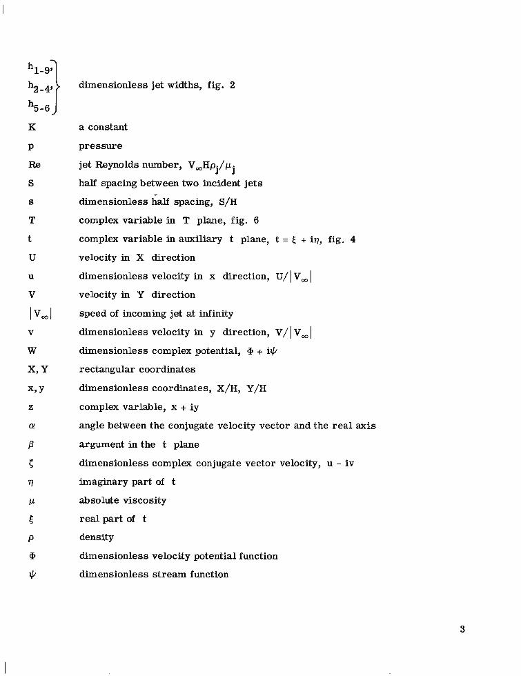
"1-9’’hn_4, dtmensionless jet widths, fig. 2

VG^K a constant

p pressure

Re jet Reynolds number, V^Sp./p..

S half spacing between two incident jets

s dtmensionless half spacing, S/H

T complex variable in T plane, fig. 6

t complex variable in auxiliary t plane, t ^ + IT], fig. 4

U velocity in X direction

u dimensionless velocity in x direction, U/1 V^V velocity in Y direction

|Vool speed of incoming jet at infinity

v dimensionless velocity in y direction, V/1 V^W dimensionless complex potential, $ + v^

X, Y rectangular coordinates

x, y dimensionless coordinates, X/H, Y/H

z complex variable, x + iy

a angle between the conjugate velocity vector and the real axis

ft argument in the t plane

^ dimensionless complex conjugate vector velocity, u iv

f] imaginary part of t

p. absolute viscosity

^ real part of t

p density

$ dimensionless velocity potential function

\p dimensionless stream function

3

Subscripts:

a atmosphere outside jet

j jet

0 refers to the origin

1, 2, 3^4, 5, 6, > these numbers refer to the points so labeled in fig. 2

7, 8, 9jinfinity

ANALYSIS

Configuration

The slot jet configuration that was analyzed is shown in figure 1. It consists of two

parallel jets each of the same width H and spaced 2S apart. The jets originate at

Y + and flow downward until they impinge on the horizontal plane at Y 0. The jet

velocities at infinity are uniform across the jet width and have the magnitude |v^| The

plane at Y 0 is normal to the jet axes. As the jets impinge on the flat plate the flow

from each jet divides into two parts. One part of each jet flows outward along the plate

to infinity. The other parts of each jet impact each other, forming a vertical column

moving upward along the positive Y axis. Since the jets are of equal width and velocity,

the flow is symmetric about the Y axis. Therefore, the configuration will be analyzed

by considering the flow in the first quadrant of the X-Y plane.

Assumptions

It is important to be aware of the basic assumptions employed in this jet analysis.

The flow is considered steady, inviscid, irrotational, and incompressible. The fluid

surrounding the jets is stationary and of constant pressure. Further, the boundary be-

tween the jets and the surrounding fluid is considered a slipline so there is no entrain-

ment of surrounding fluid into the jet. As a result, the slipline is also a streamline.

This slipline boundary will hereafter be referred to as the free streamline. The assump-

tion that the pressure along the free streamline is constant requires not only stationary

surrounding fluid but also neglect of gravity effects. The neglect of gravity in the jet0

flow solution is equivalent to saying that the jet Froude number Voo/gH, which is the

ratio of inertia forces to body forces, is large.

4

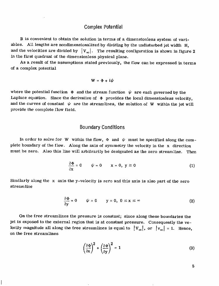
Complex Potential

It is convenient to obtain the solution in terms of a dimensionless system of vari-ables. All lengths are nondimensionalized by dividing by the undisturbed jet width H,and the velocities are divided by V^ The resulting configuration is shown in figure 2in the first quadrant of the dimensionless physical plane.

As a result of the assumptions stated previously, the flow can be expressed in termsof a complex potential

W $ + ii^

where the potential function $ and the stream function i// are each governed by theLaplace equation. Since the derivative of $ provides the local dimensionless velocity,and the curves of constant ^ are the streamlines, the solution of W within the jet willprovide the complete flow field.

Boundary Conditions

In order to solve for W within the flow, $ and ^ must be specified along the com-plete boundary of the flow. Along the axis of symmetry the velocity in the x directionmust be zero. Also this line will arbitrarily be designated as the zero streamline. Then

9+/-= 0 i^ 0 x 0, y ^ 0 (1)3x

Similarly along the x axis the y-velocity is zero and this axis is also part of the zerostreamline

-8*!’ 0 i// 0 y 0, 0 < x ^ (2)9y

On the free streamlines the pressure is constant; since along these boundaries thejet is exposed to the external region that is at constant pressure. Consequently the ve-locity magnitude all along the free streamlines is equal to |VoJ, or (v^[ 1. Hence,on the free streamlines

(^ . (^ l (3)W \ay/

5

To determine the magnitudes of the stream functions on the free streamlines the

Cauchy-Riemann equation

^L a$ -v9x 9y

is applied. Then between points 5 and 6 on figure 2

^ 0 f^ -v dx f^ -1 dx -^.6 ^^ (4)

In a similar manner

^1-2 ^1-Q <5)

The asymptotic coordinates for the jet at its origin in figure 2 are

ho 4x s + s + yo (6)2 2

hq 4x. s s y, (7)

2 2 4

The amount of mass flow from each jet which is deflected toward the axis of symmetry,and toward the outside is not known a priori. As a result, the coordinates for points 1

and 5 cannot be completely specified in advance. Therefore, the remaining coordinates

for the free streamlines are expressed implicitly as

^ Ve^ y5 (8)

x^ y^ h^g(s) (9)

The functions hr_c(s) and h,_q(s) as well as the shape of the free streamlines (the con-

stant i^ and i^- lines) must be determined.

Conformal Mapping Method

The derivative of the potential W provides the complex conjugate of the vector ve-

locity within the jet flow region.

6

^. u iv ^dz

By integrating, it is evident that the physical plane is related to the potential plane bymeans of an integration involving ^

z y^"1 dW + constant (10)

The solution of equation (10) to determine the jet configuration in the z plane subject tothe boundary conditions discussed in the previous section will be carried out by a tech-

nique whose development is generally attributed to Helmholtz and Kirchhoff (see ref. 1).As will be shown subsequently, the flow region in the W and ^ planes is known fromavailable information. In order to integrate equation (10) these W and ^ regions are

mapped conformally into an intermediate t plane. Once the W(t) and ^(t) transforma-tion functions are known, they can be substituted into equation (10) and z as a function

of t can be computed. Then the z(t) function can be used to express W(t) and C(t) im-plicity in terms of z and thus solve the problem.

Hodograph ^ to auxiliary t plane transformation. The hodograph (^ u iv)plane is shown in figure 3. The free streamlines (’^1 0 and V^ i-) because of their

property of having constant velocity magnitude are represented by the arcs 1-2 and 4-5of the unit circle in the hodograph. The flow along the horizontal wall where v 0 is

represented by 7-a-8-9, while the axis of symmetry where u 0 becomes the line 6-7on the ^ plane. It should be noted that there are two stagnation points. Point 8 rep-resents the coordinate about which each jet divides. Point 7 represents the stagnationpoint formed by the portions of each jet that impact at the origin of the z plane. In the

z plane, point 8 may for some conditions fall on the axis of symmetry between 6 and 7rather than lying on the real axis. This occurs when the spacing s is sufficiently small

and will be discussed in detail in the section RESULTS AND DISCUSSION.The domains representing the jet flow regions in the z and ^ planes are simply

connected schlicht (sometimes referred to as simple) domains whose boundaries consist

of more than one point. By Riemann’s mapping theorem (ref. 3) these two domains are

conformally equivalent and the conformal map ^ ^(z) exists. Strictly speaking ^(z)need be conformal only within the domain and not at every boundary point. Throughoutthis report we will follow the custom that the mapping will be referred to as conformaleven though there are points on the boundary where this is not true.

Since the ^ domain has the properties described in the previous paragraph it in

turn can be mapped conformally onto the simply-connected schlicht domain consisting ofthe interior of the unit semicircle in the auxiliary t-plane as shown in figure 4. The

mapping is performed so that the free streamline arcs 1-2 and 4-5 transform to the half

7

circle with unit radius, and the straight line segments 6-7 and 7-8-9 go respectively into

-1 < t < 0 and 0 < t < 1 on the real axis. This is accomplished by the transformation

(ref. 4)

.1/2(. 0 ^ |t| < 1

^t (t A) (11)

At 1 0 == |A| 1

where A corresponds to the distance in the t plane between the stagnation points 7

and 8. The points t 0 and t A where ^ 0 represent the two stagnation points.

This transformation has caused the straight lines which compose the multiple piece

boundary 6-7-8-9 to become one straight line segment in the t plane.

The conjugate velocity ^ is now in terms of t, the variable in which equation (10)will eventually be integrated.

Complex potential W to auxiliary t plane transformation. The complex potential

W $ + ii^ must also be expressed in terms of t before the integration can be per-

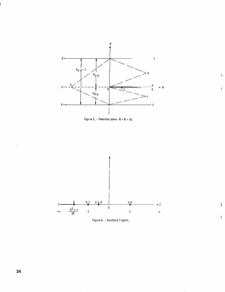
formed. The flow region in the W plane is shown in figure 5. The streamlines are

parallel and the free streamlines form the upper and lower boundaries of the region at

^ h, Q and hc c, respectively. The flow can be visualized as entering at the left and

flowing toward the right between the free streamlines. The dotted streamline 3-8 is the

line between the two portions the jet divides into as a result of the impact. The value of

$ at point 8 is arbitrarily taken as zero; this is permissible as will be shown.

The well-known Schwarz-Christoffel transformation (ref. 5) can be used to map a

polygon onto the upper half plane. The flow region in the W plane can be considered a

degenerate form of the dashed polygon, shown in figure 5. The points 5-6, 1-9, and

2-3-4 are formed by taking points c, d and e, respectively to infinity. In traveling

around this polygon the change in exterior angle at each of points 9-1, 2-3-4, and 5-6 is

+ir and the change at point 8 is -v for a total change of 2v. Therefore, we use the de-

generate Schwarz-Chrostoffel function

/ B(T TjdTW(T) ------------------- + r (12)

T Ti_g)(T T2_3_4)(T T5_g)

to conformally map the interior of the region in the W plane onto the upper half T plane

shown in figure 6. The polygon in the W plane is unfolded so that its entire boundary

becomes the real axis in the T plane. Point 7 in the W plane is transformed to infinity

in the T plane.

The final step of mapping the W plane into the t-plane is performed by the function

8

T 1 ^ 1^ (13)2 ^ t/

which conformally maps the upper half T plane into the unit semicircle shown in fig-ure 4. Once the necessary constants are determined for the W mapping function in

equation (12), W(t) can be found by eliminating T by use of equation (13). Then W(t)and S(t) from equation (11) can be substituted into the z equation (10) so it can be inte-

grated.

Using partial fractions and simplifying the notation by letting Tq o_4 be T,, the

integrand of equation (12) becomes (note that there are sufficient degrees of freedom in

the transformation so that Ti n and Tc o have been fixed at -1 and +1, respectively):

_________TiT8_________ _C_^^_

^^_ (14)(T Ti_n)(T Tg_o_4)(T Tg_g) T + 1 T To T 1

where

1 + TnC -____-

2(1 + T3)

TK ^D -__2T1 ^

1 ToE ----8-

2(1 T3)

The position Tn can be found in terms of the parameter A which is the position of t,,

on figure 4. From equation (13)

^ K^i) (15)

The quantity To can also be found in terms of A. From equation (13)

Tg 1 ftg + ^\ (16a)3 3 V 3 W

From equation (11) at point 3, ^ i so that

9

^(to A)i -"--"--- (16b)

^ 1

If to is eliminated from (16a) and (16b) the result iso

T, A 2A 1 (17)2

Equations (15) and (17) are substituted into C, D, and E to give

C -i- (18a)2A

D --2-- (18b)A(A 3)

E ^A + ^ (18c)2A(A 3)

Equation (14) is substituted into the integral of equation (12) and the integration is carried

out to give

W BC ln(T + 1) + BD ln(T To) + BE ln(T 1) + K

The constant K is determined from the arbitrarily imposed condition W 0 at T To.This gives

W =Bcfln(T+ 1) ln(Tg + 1)] + BD[ln(T To) ln(Tg To)] + BE[m(T 1) ln(Tg 1)1 (19)

The coefficients will now be related to the jet widths hg_g and h- o. To do this

the imaginary part of W is utilized

i^=Bc[arg(T+ 1) arg(Tg+ l)]+BDfarg(T To) arg(Tg To)] +BEfarg(T 1) arg(Tg 1)1

Since To + 1, To To, and To 1 are all real and negative, this becomes

^ Bc[arg(T + 1) ff] + BD[arg(T To) v} + BE[arg(T 1) 7r] (20)

10

In the region between Tg_g and T^, ^ 0 and T > 1 > T, > -1. Hence

0 BC(0 TT) + BD(0 7r) + BE(0 ir)

or

BC + BD + BE 0 (21a)

On the free streamline between points 4 and 5, equation (4) gives ^4 1- -h,- , andsince 1 > T > To > -1,

-hg_g BC(0 v) + BD(0 ir) + BE(TT -n)

or

h^ fiBC + BD --- (21b)71-

On the free streamline between points 2 and 1, equation (5) gives i^ h, q, andsince l > To > T > -l

h^_g BC(0 7]-) + BD(7T 77-) + BE(7T IT)

or

hi aBC --1^9 (21c)

7T

From continuity

hl-9 + VG 1 (22)

Equations (21a), (21b), (21c), and (22) give

hi n heBC -LZ BD and BE o"b (23)

IT n TT

From the relation B 1/irD, B can be found by using D from equation (18b)

B A(A 3) (24)2ff

11

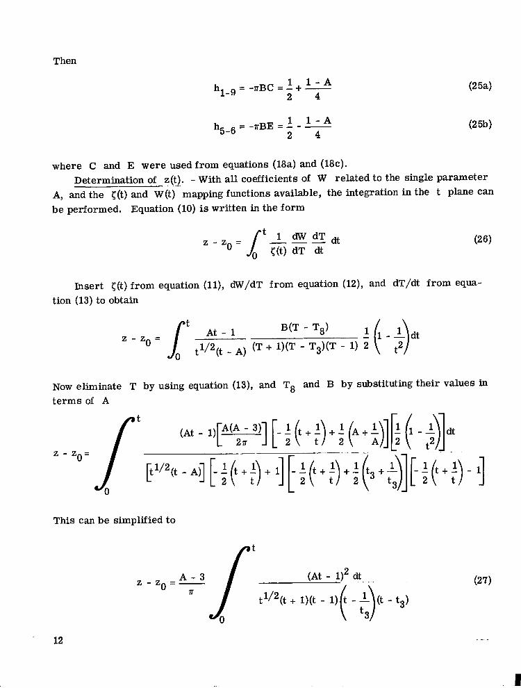
Then

h< ^-^rBC l+ ^- A (25a)

1-H 2 4

h. -TTBE A 1-^ (25b)5-6 2 4

where C and E were used from equations (18a) and (18c).Determination of z(t). With all coefficients of W related to the single parameter

A, and the ^(t) and W(t) mapping functions available, the integration in the t plane can

be performed. Equation (10) is written in the form

z z_ y’-L ^ ^ dt (26)0 JQ S(t) dT dt

Insert ^(t) from equation (11), dW/dT from equation (12), and dT/dt from equa-

tion (13) to obtain

z z, r ^i- B(T ^ i fi 4t7o t17^ A) (T + 1)(T ^ 1) 2 \ t2/

Now eliminate T by using equation (13), and Tg and B by substituting their values in

terms of A

/ (At 1)?^ ^j f- A ft . l^ l /A ^M 1 (l A dti 2, ]\_ 2 \ t 2 \ AJ] 2 \ ^tf

7 ’7 ^^

rtv^ A^ f- i ft . i^ iT 1 ^ 1^ 1^^ [- l ^t . l\ ^L -] \. 2 \ t ] 2\ t 2\3 t^ i 2\ i ]

This can be simplified to

rz z^ A^ / (At ^ ^

(27)

/ tV^t + iKt D^t A-Vt tg)

^ V t3/12

1

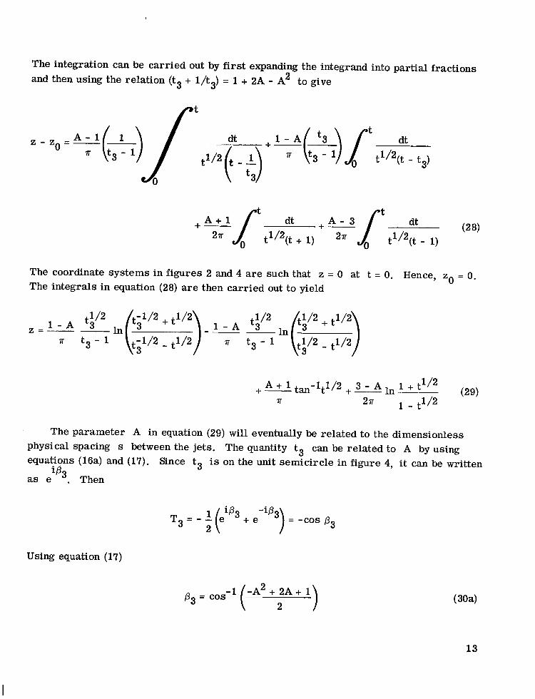
The integration can be carried out by first expanding the integrand into partial fractionsand then using the relation (tg + 1/tg) 1 + 2A A2 to give

r^ ^ ^J.(_+/- \ I _^t___

^l^/_t3 ^ />t dt- ^ 1) I W A - ^3 ^ t^t t^)

</ \ W

. Aj^ /t dt , A^3 />t dt

21r ^ tV^t . 1) 2^ t1/2^ 1)

The coordinate systems in figures 2 and 4 are such that z 0 at t 0. Hence, z.. 0.The integrals in equation (28) are then carried out to yield

1 A ^ As172-^ 1 A ^ (^ - ^\z 1-" -&-- ln( -3------ 1 A -3__ in /-3______v t3 l Vt-^ t1/2 / v t3 l Vt1/2- !1/2 /

\ ’ / \ o /

,. A_tA tai.^t1/2 + l^-A in l-t^ (29)TT 2ir

^ ^1/2

The parameter A in equation (29) will eventually be related to the dimensionlessphysical spacing s between the jets. The quantity to can be related to A by usingequations (16a) and (17). Since tg is on the unit semicircle in figure 4, it can be written

if3nas e ". Then

1 / i^g -1/3.AT3 -(e + e 3 -cos ^3

\ /

Using equation (17)

,3 cos-1 (-A2^ ’) (30a)

13

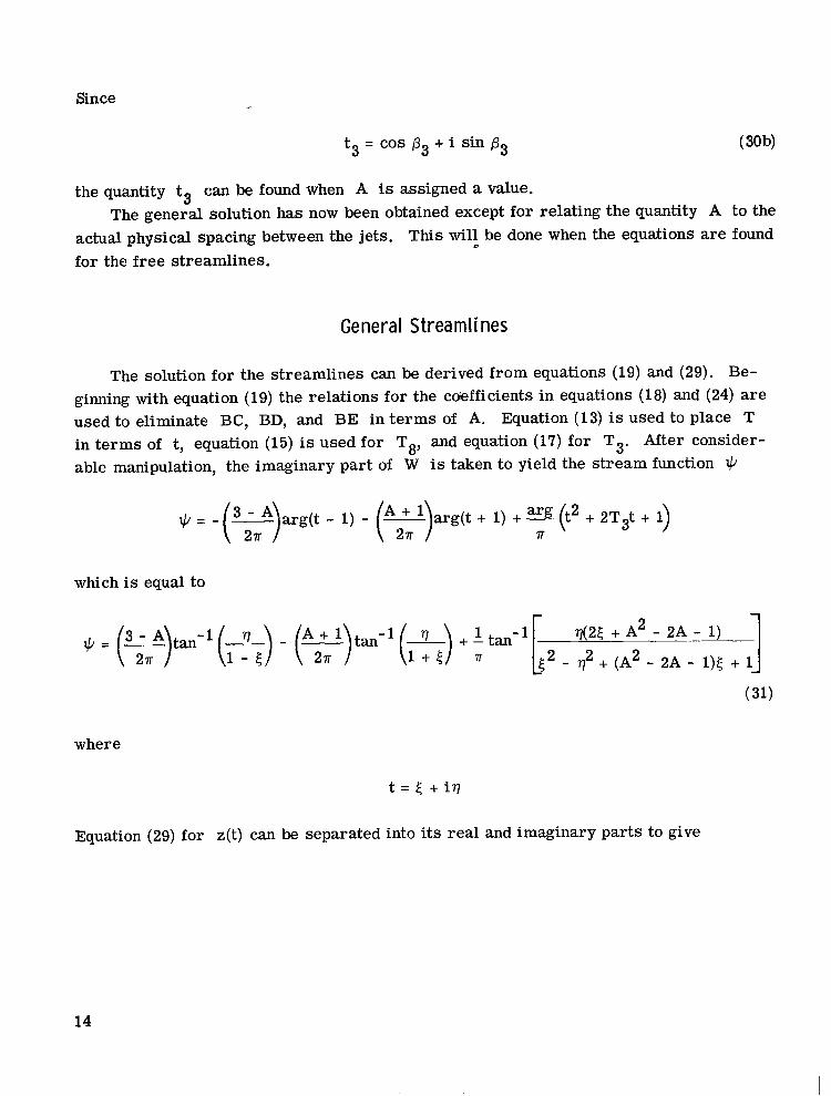
Since

tg cos /3o + i sin /3g (30b)

the quantity to can be found when A is assigned a value.

The general solution has now been obtained except for relating the quantity A to the

actual physical spacing between the jets. This will be done when the equations are found

for the free streamlines.

General Streamlines

The solution for the streamlines can be derived from equations (19) and (29). Be-

ginning with equation (19) the relations for the coefficients in equations (18) and (24) are

used to eliminate BC, BD, and BE in terms of A. Equation (13) is used to place T

in terms of t, equation (15) is used for Tg, and equation (17) for Tg. After consider-

able manipulation, the imaginary part of W is taken to yield the stream function ^V, -/l^argd 1) f^arg^ + 1) +^ (t2 + 2Tgt + l)

\ 2-ir \ 2ir v

which is equal to

^ t^tan-1 l-H-\ fA-LlVan-1 f^-\ , 1 tan-1 ---^ . A2 2A 1)

\ 27T / \l U \ 27T / \1 + U 7T ^ ^ ^ ^2. 2A 1)^ + 1_

(31)

where

t ^ + i?7

Equation (29) for z(t) can be separated into its real and imaginary parts to give

14

, l + ltl -^ltl^ cosf^ , 2|t| l/2 cos(^)x 3 ^1 in ^ . ^tan-1 --_____W

Y 4ff / l + ltl ^ltl^ cos^ V 27r / ^ N\2/_ L

i; / /9 /3 + /3.X /, /2 ^ j6A/2 t 1/2 sin ---3\ /2 t 1/2 sin ---" N

+ t?^_ _________2_ tar^1_________2_ (32)

^ ^ \ 1 |t| / ^ \ 1 I1! /

1^ ^ -.

il 2|t| l/2 sin^| /l . ltl ^ltl^ sin ^Y;; y (^\t^-1 ^ .. ^ logf-----------,---2-}\ ^ 1 M V 4^ Vl + ltl ^ltl^ sin^\ v-

1 /2 /’3 ^1 + t + 2 t 1/2 cos ---"’_____\ 2 /

l . ltl ^ltl^ cos ^3)\ + ^- log ---------v 2 / (33)

27r 1 /2 fl3 + ^\1 + t + 2 t 1/2 cos ---_____________\ 2 /

i . ltl altl^ cos^)\ 2 /

Equations (31) to (33) represent a set of parametric equations for determining ^ as

a function of x and y. The i^ constant lines can be found by determining the f, and

77 values from equation (31) for a specific i^. Then these values of ^ and i] are sub-

l stituted into equations (32) and (33) to obtain the corresponding x ajid y coordinates.

Free Streamlines

Equations (32) and (33) become the equations for the free streamlines by substituting

|t| 1 which gives

15

i.

/I + cos &\x ^A In _____n .^ (34)

47r V l cos ^ / 4

\ 2/-

/’3 ^3\l + cos^1 cosf^ , /l . sinA

y -L m \ 2 ; 3^A /Aj_A\ ,J____2 ^ (35)2ff

l . cos^) 4 V 4- / V - f /\ 2 / L x 2/-1

/’8 + ^^\1 cos(---"

\ 2 /

for

ir ^ ^ > /3g

and

(I + cos Ax 3-^-A In ----2 | + AJ-A + i (36)

477 cos ^ / 4

2/_

//3, i8\1 + cos -"--

\ 2 / J/^ ^\ / /A’

1 cos /l + sin p\y ^ ln ----L^_^L ^ 3^A

/Aj_l\ iJ____2_ \^2T

l . cos^) 4 ^^. V1 81^/_____\ 2 /

//3o + ^\1 cos -"--

\ 2 /_

16

{ for

1. ;3g s /3 ^ 0

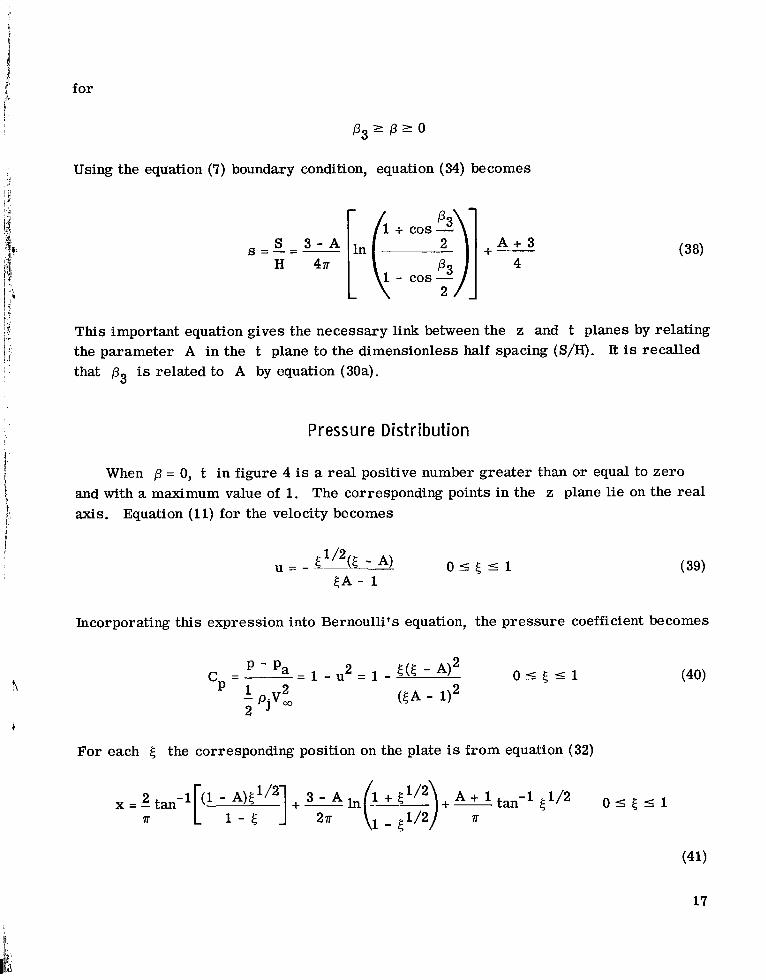
Using the equation (7) boundary condition, equation (34) becomes

I /l ^ cos ^\"I s ^ -^A In _____2- 1 + AJ-3 (38)t H 4ir I ;3, / 4I \1 cos -3 /

\ 2 /_

This important equation gives the necessary link between the z and t planes by relating

the parameter A in the t plane to the dimensionless half spacing (S/H). It is recalled

that /3o is related to A by equation (30a).

Pressure Distribution

When /3 0, t in figure 4 is a real positive number greater than or equal to zero

and with a maximum value of 1. The corresponding points in the z plane lie on the real

axis. Equation (11) for the velocity becomes

1/2u ^--(t-lA) 0 < ^ ^ 1 (39)

^A 1

Incorporating this expression into Bernoulli’s equation, the pressure coefficient becomes

Cp pa^ l u2= l ^ A)2 0 - ^ 1 (40)

’ p

1?^ (,A 1)2

For each ^ the corresponding position on the plate is from equation (32)

x ^ tan-^^ ^^I .^A ln^ ^^V A^A tan-1 ^/2 0 - ^ 1TT L 1 ^ J 2lT \^ ^./2f 7T

(41)

17

1

RESULTS AND DISCUSSION

As shown in the analysis, the configuration of the jet flow depends on only one pa-

rameter, the dimensionless half spacing (S/H) between the jets. The analytical solution

came out more conveniently in terms of A which is related to S/H by means of equa-

tions (38) and (30a). The results will consist of a set of plots for various S/H of the

free streamlines, the wall pressure coefficient, and some of the streamline patternswithin the jets.

To compute the free streamlines, a value for A is first chosen. The quantity ;3ois then found from equation (30a) and the jet spacing is found from equation (38). Equa-tions (34) to (37) can then be used to compute the free streamlines. The pressure coef-

ficient is found by letting ^ vary between 0 and 1 in equations (40) and (41). This gives

C and the corresponding x values along the wall.The streamline pattern within the jets is computed from equations (31) to (33). An

arbitrary pair of ^ and f] values are chosen which correspond to a point within the unit

semicircle of figure 4 (i. e. |t v ^ + rr < 1). The value of the stream function is

then computed from equation (31). The physical coordinates x and y corresponding to

this value of ip are then found from equations (32) and (33). By doing this for numerous

[t[ points within the unit semicircle, the entire streamline pattern can be mapped.

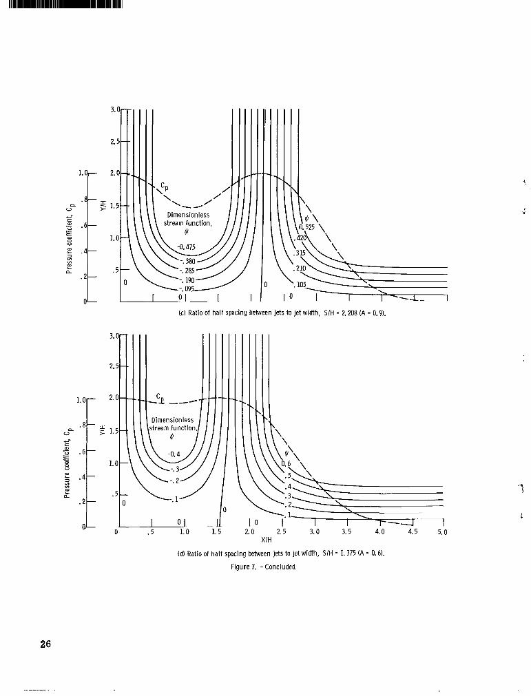
Figure 7 shows the results for several jet spacings corresponding to positive values

of A. For positive A the stagnation point 8 lies on the x axis as shown in figure 2.Figure 7 (a) shows the configuration for a large spacing between jets; in this case the

spacing between the two jets is about 6 jet widths (half-spacing S/H 3. 132). Each jet

acts practically independently and divides so that half of the flow goes toward x +o

and half toward x 0 where the portions of the two jets merge to form a jet one width

wide moving toward y +. The incident fluid stream is not influenced by the plate

until it is within about two jet widths from the plate.

The pressure coefficient in figure 7 (a) is unity at the two stagnation points where

there is complete recovery of the velocity energy for the inviscid conditions considered

here. At X/H 5, C 0, indicating that the flow has completely turned and the veloc- /"i

ity magnitude along the wall is V^The other three parts of figure 7 show similar jet patterns as the jet spacing is de-

creased which causes the stagnation point 8 to move closer to the stagnation point 7.Figure 7(d) shows a typical streamline pattern, and in this instance in the region of

X/H 0. 8 the C decreases only a small amount from unity. This shows that the re-

gion near the wall between the two stagnation points is essentially a stagnation region.

The low velocity in this region is evidenced by the wide spacing between the streamlines

ip -0. 1 and i^ 0.

Figure 8 shows the flow configuration when A 0 which causes all the stagnation

18

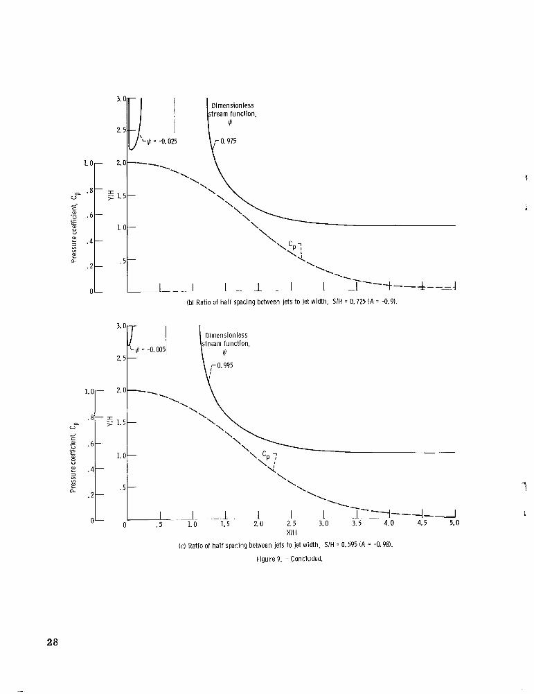
^points to coincide at the origin. This corresponds to a half spacing of 1. 379 jet widths.

? A further decrease in jet spacing below that of figure 8 produces the series of flowpatterns in figure 9. Here the dividing streamline \p 0 ends at a stagnation point alongthe y axis of symmetry. Part of the jet is turned and moves back toward y + with-

out penetrating very close to the wall. As the spacing is further decreased the streamflowing back along the y-axis is diminished in width and is formed further away from the

wall. m figure 9(c) there is practically no backward circulation and the two jets have

I; almost merged to form a single jet of width 2H centered about the y-axis.

It. The percent of recirculation up the y-axis, as a function of dimensionless half spac-ji ing (S/H), can be determined from equations (25b), (30a), and (38). A plot of the per-

centage recirculation 100 hg_ g as a function of S/H is shown in figure 10. Note that

when S/H 0. 5, the two jets have merged into a single one and there is no recirculatingflow.

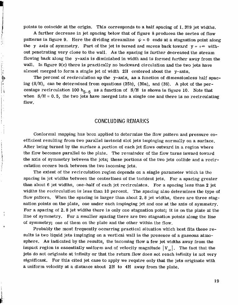
CONCLUDING REMARKS

Conformal mapping has been applied to determine the flow pattern and pressure co-

efficient resulting from two parallel inviscid slot jets impinging normally on a surface.After being turned by the surface a portion of each jet flows outward in a region wherethe flow becomes parallel to the plate. The remainder of the flow turns inward toward

the axis of symmetry between the jets; these portions of the two jets collide and a recir-

culation occurs back between the two incoming jets.

The extent of the recirculation region depends on a single parameter which is the

spacing in jet widths between the centerlines of the incident jets. For a spacing greaterthan about 6 jet widths, one-half of each jet recirculates. For a spacing less than 2 jet

widths the recirculation is less than 10 percent. The spacing also determines the type of

flow pattern. When the spacing is larger than about 2. 8 jet widths, there are three stag-nation points on the plate, one under each impinging jet and one at the axis of symmetry.For a spacing of 2. 8 jet widths there is only one stagnation point; it is on the plate at the

line of symmetry. For a smaller spacing there are two stagnation points along the line

of symmetry; one of them on the plate and the other within the flow.Probably the most frequently occurring practical situation which best fits these re-

sults is two liquid jets impinging on a vertical wall in the presence of a gaseous atmo-sphere. As indicated by the results, the incoming flow a few jet widths away from the

impact region is essentially uniform and of velocity magnitude V The fact that the

jets do not originate at infinity or that the return flow does not reach infinity is not verysignificant. For this cited jet case to apply we require only that the jets originate with

a uniform velocity at a distance about 2H to 4H away from the plate.

19

L

The pressure distribution along the plate for the cited liquid jet in air is of practical

value. Portions of the pressure distribution can be used for calculating the boundary

layer and heat transfer between the plate and jet. In the case where 1 < S/H < 2. 5, the

pressure coefficient should be valid from X/H 0 to X/H ^ 4. Beyond X/H ^ 4, the

entrainment effects and wall boundary layer become significant and the flow approaches a

viscous wall jet. As the jet spacing is increased beyond 2. 5; the entrainment effects on

the recirculating portion of the jet, at small X/H, will significantly affect the C in-

validating the inviscid analysis in the region of the stagnation point (point 7) at X 0.

When the jet and surrounding fluid are the same, entrainment effects can invalidate

the C solution throughout the stagnation zone regions. The incoming jet interacts with

the recirculating portion to retard the incoming jet flow. As a result the C will be /

less than 1 at the stagnation points. This has been experimentally shown in reference 6.

The analytical techniques used to solve the current jet flow can be used for the solu-

tion o"f any problem governed by Laplace’s equation with boundaries consisting of straight

surfaces and free streamlines. For instance, the solidification of a flowing liquid on a

cold surface has recently been analyzed in reference 7 using these techniques.

Lewis Research Center,National Aeronautics and Space Administration

Cleveland, Ohio, September 25, 1968,129-01-07-07-22.

REFERENCES

1. Milne-Thomson, L. M. Theoretical Hydrodynamics. The Macmillan Co. 1938.

2. Gardon, Robert; and Akfirat, J. Cahit: The Role of Turbulence in Determining the

Heat-Transfer Characteristics of Impinging Jets. Int. J. Heat Mass Transfer, vol.

8, Oct. 1965, pp. 1261-1272.

3. Nehari, Zeev: Conformal Mapping. McGraw-Hill Book Co. me. 1952.

4. Birkhoff, Garrett; and Zarantonello, E. H. Jets, Wakes, and Cavities. Academic

Press, Inc. 1957.

5. Churchill, Ruel V. Complex Variables and Applications. Second ed. McGraw-Hill

Book Co. me. 1960.

6. Gardon, Robert; and Akfirat, J. Cahit: Heat Transfer Characteristics of Impinging

Two-Dimensional Air Jets. J. Heat Transfer, vol. 88, no. 1, Feb. 1966, pp. 101-

108.

20

J

^7. Siegel, Robert: Conformal Mapping for Steady Two-Dimensional Solidification on a

Cold Surface in Flowing Liquid. NASA TN D-4771, 1968.fI

IIit!’

1.^!1*!

i1^

!I

21

L

Velocity of in-coming jetat

infinity,

-^ V

Width of ^s^\.undisturbed I’C^ ^m ^^^^1

jet, -^-s, f ^’^>^. "r "^ ^"4

^So ^>’

^s--^ ^^^ Spacing between two.>< ^^ /, ’<^^ incident jets, 2S

Figure 1. Impingement of two parallel jets on horizontal plane.

Dimensionlesshalf spacing,

y^v ^^6 5 Dimensionless Dimensionlessjet width, jet width,

"5-6 "2-4 1

^ Dimensionlessstream function,

’"4-5’ -"5^ ’^Point where ^ 1’1-2’+ "1-9v 0 on h^.gfree stream- \

\ line, b -^ / N^______^^----I ---^ ""---------^------^ \ x

’-Point of maximumvelocity along wall, a

figure 2. Jet flow in first quadrant of dimensionless z-plane.

22

1

.Velocity

w y -yX

^!.’i 4,3,2

^1’!isi’t

^ ----^ ^-------u"i

I

Figure 3. Hodograph plane I, u iv.

t

T’

It ^---~^^3,4

5,6 /_______7 / ^8 9\1______.- ^Figure 4. Auxiliary t-plane, $+ iii ’Itle’P.

23

Ill

2 t >-h2. / ^/ ^1-9 ^>d

^/ ^

J3-^ ^^^^^ 93--<.-^-----;----8 ’^ ^ -g ^

’^ h5-6 ^^>c4------------r ^^- -- ’’""---------5

Figure 5. Potential plane W $ + i(t.

8 9,1 2,3,4 5,67-----.---------^------------’s--------- ^7 1

^- -.

Figure 6. -Auxiliary T-plane.

24

^A

t3.0|-

^ Dimensionless

!’ stream function,2.5- ip,

^-0.49875

t T ""^ /""^t "- ’’-I L’ K / \I g ’ \ ^ / / \\I .4 \ \ / / ^ -0.50125^ \ \tt I v^^, ^^^/ Y^_^a - ’ ^-^ ^\-| ,L ___^|j (a) Ratio of half spacing between jets to jet width, S/H 3.132 (A 0.995).

I ’-"r Dimensionlessstream function,

2.5- ’.

^ ^-0.495 ^ ((,= 0.505

I ’"r 2-0’^ ^--^i. \ /’ \

^ \-8 -= \ / \

^ ? 1.5- \ / \5 A \ \ / / \ \ Cn-6 \ \ / / \ \P7I 4

1’0-’ \ v-^ / \ \s ^___________. .. 5- ^----------0 ___________I v^

0 .5 1.0 1.5 2.0 2.5 3.0 3.5 4.0 4.5 5.0X/H

(b) Ratio of half spacing between jets to jet width, S/H 2.698 (A 0.98).

Figure 7. Jet configurations for sufficiently large spacings so that all stagnation points are on wall.

25

I;

3.0,-T-

2.5-

1. 2.0 .-- --,

^’^ / ^\8--

5- ^^ \>- ’> \^- Dimensionless ili \.5 6 stream function, / / \( 575 \

I 5 \, Y^--23S^^/ y \ .210^^S^’20 V^-.190-^,^ \

105 ^^^-.^^^--.095----^ ~~---I~~~^^.----------0 \ O l^ 1^~------ 1^-4-,---1

(c) Ratio of half spacing between jets to jet width, S/H 2.208 (A 0.9).

3.0-

2.5-

Dimensionless ^i; stream function, \

^ \ ’r \\\^ \\\ / / / / \ \\ \s 6 _\ \\\^y// / \ \\\\ \

2 ’o ^-1 \ ^^’^^^^lo ^-^..^ ^__________o _______o_\ ll o I""-T---I ’" 1~---J---1

0 .5 1.0 1.5 2.0 2.5 3.0 3.5 4.0 4.5 5.0X/H

(d) Ratio of half spacing between jets to jet width, S/H 1.775 (A 0.6).

Figure 7. Concluded.

26

II

I 3()

;’ 2 5 O’l’ension-1< less stream;lt function,

|, ^

I -8 -^ A // / \V0 75s ^ ^AW// \ \YvI s -6 ’^ / v Vv6^P g 1.0- / \ \ .5 \ "S<^

|" 0 .5 LO 1.5 2.0 2.5 3.0 3.5 4.0 4.5

I:’ X/H

|( Figures. Jet configuration when all stagnation points coincide. Ratio of half spacing between jets1; to jet width, S/H 1.379(A=0>.

Dimensionlessstream function,

1i3oi"

2.5

o o 1 --^^rj0 .5 1.0 1.5 2.0 2.5 3.0 3.5 4.0 4.5

X/H

(a) Ratio of half spacing between jets to jet width, S/H 0.997 (A -0.6).

Figure 9. Jet configuration when jet spacing is sufficiently small so that there is a stagnation pointon the line of symmetry.

27

t

i

3.0H-Dimensionless

(stream function.(?

2.5 -/

j’^-ili’ -0.025 \ -0.975v

2.0--^^ \

0&8- 5- ^^K"s \ ^^^| .6 \ ^^^^^^^i 1.0- \

\\4\ L,,\\

25

"^o

_____1 ^T’~-^--4.-=-l

(b) Ratio of half spacing between jets to jet width, S/H 0.725 (A -0.9).

^rr Dimensionless/ (stream function,’-ill -0.005 \ in

2.5-\ /-0.995

.- 8-

^ - ^ ^K| -6- ^^_________________________% i. o \ ^ -78 \

.4- \C5 \

^ .2--5 "^^1 ^1~-~:-1----^---^0 .5 1.0 1.5 2.0 2.5 3.0 3.5 4.0 4.5 5.0

X/H

(c) Ratio of half spacing between jets to jet width, S/H 0.595 (A -0.98).

Figure 9. -Concluded.

28

’?I

50i- ^-------

40- /

| 30- /g- /cz’ /

/

^ /

I 20- //

.5 1.0 1.5 2.0 2.5 3.0 3.5Half spacing between jets, S/H

Figure 10. Percent of flow recirculating back along Y-axis as function of half spacingbetween jets.

,;

\

{ NASA-Langley, 1968 12 E-4528 29

^;’

NATIONAL AERONAUTICS AND SPACE ADMINISTRATION POSTAGE AND FEES PAID

r> r- WS.A/- NATIONAL AERONAUTICS ANDWASHINGTON, D.C. 20546 SPACE ADMINISTRATION

OFFICIAL BUSINESS FIRST CLASS MAIL

.N]

^f

If Undeliverable (Section 158POSTMASTER, postal Manual) Do Not Return

"The aeronautical and space activities of the United States shall beconducted so as to contribute to the expansion of human knowl-edge of phenomena in the atmosphere and space. The Administrationshall provide for the widest practicable and appropriate dissemination

of information concerning its activities and the results thereof"--NATIONAL AERONAUTICS AND SPACE ACT OF 1958

NASA SCIENTIFIC AND TECHNICAL PUBLICATIONS

TECHNICAL REPORTS: Scientific and TECHNICAL TRANSLATIONS: Information

technical information considered important, published in a foreign language considered

complete, and a lasting contribution to existing to merit NASA distribution in English.knowledge.

SPECIAL PUBLICATIONS: Information

TECHNICAL NOTES: Information less broad derived from or of value to NASA activities.

in scope but nevertheless of importance as a Publications include conference proceedings,contribution to existing knowledge, monographs, data compilations, handbooks,

sourcebooks, and special bibliographies.TECHNICAL MEMORANDUMS:Information receiving limited distribution TECHNOLOGY UTILIZATION ^because of preliminary data, security classifica- PUBLICATIONS: Information on technologytion, or other reasons, used by NASA that may be of particular

interest in commercial and other non-aerospaceCONTRACTOR REPORTS: Scientific and applications. Publications include Tech Briefs,technical information generated under a NASA Technology Utilization Reports and Notes,contract or grant and considered an important ^j Technology Surveys.contribution to existing knowledge.

Details on the availability of these publications may be obtained from:

SCIENTIFIC AND TECHNICAL INFORMATION DIVISION

NATIONAL AERONAUTICS AND SPACE ADMINISTRATIONWashinston, D.C. 20546