I/O-Efficient Algorithms for Computing Contour Maps on Terrains

Pankaj K. Agarwal∗

CS DepartmentDuke University

Durham, NC

pankaj@cs.duke.edu

Lars Arge†

MADALGO‡

CS Department

University of Aarhus

Aarhus, Denmark

large@daimi.au.dk

Thomas Mølhave§

MADALGO

CS Department

University of Aarhus

Aarhus, Denmark

thomasm@daimi.au.dk

Bardia Sadri¶

CS Department

University of Toronto

Toronto, ON, Canada

sadri@cs.toronto.edu

Abstract

A terrain M is the graph of a continuous bivariate function. We assume that M is representedas a triangulated surface with N vertices. A contour (or isoline) of M is a connected componentof a level set of M. Generically, each contour is a closed polygonal curve; at “critical” levelsthese curves may touch each other or collapse to points. We present I/O-efficient algorithms forthe following two problems related to computing contours of M:

(i) Given a sequence `1 < · · · < `s of real numbers, we present an I/O-optimal algorithm thatreports all contours of M at heights `1, . . . , `s using O(sort(N) + T/B) I/Os, where T isthe total number of edges in the output contours, B is the “block size,” and sort(N) isthe number of I/Os needed to sort N elements. The algorithm uses O(N/B) disk blocks.Each contour is generated individually with its composing segments sorted in clockwiseor counterclockwise order. Moreover, our algorithm generates information on how thecontours are nested.

(ii) We can preprocess M, using O(sort(N)) I/Os, into a linear-size data structure so that allcontours at a given height can be reported using O(logB N + T/B) I/Os, where T is theoutput size. Each contour is generated individually with its composing segments sorted inclockwise or counterclockwise order.

∗Supported by NSF under grants CNS-05-40347, CFF-06-35000, and DEB-04-25465, by ARO grants W911NF-04-1-0278 and W911NF-07-1-0376, by an NIH grant 1P50-GM-08183-01, by a DOE grant OEG-P200A070505, and bya grant from the U.S.–Israel Binational Science Foundation. Supported by NSF under grants EIA-01-31905, CCR-02-04118, and DEB-04-25465, by an ARO grant W911NF-04-1-0278, and by a grant from the U.S.–Israel BinationalScience Foundation.†Supported in part by the US Army Research Office through grant W911NF-04-01-0278, by an Ole Roemer

Scholarship from the Danish National Science Research Council, a NABIIT grant from the Danish Strategic ResearchCouncil, and by the Danish National Research Foundation.‡Center for Massive Data Algorithmics — a Center of the Danish National Research Foundation.§Supported in part by an Ole Roemer Scholarship from the Danish National Science Research Council, a NABIIT

grant from the Danish Strategic Research Council, and by the Danish National Research Foundation.¶Work performed primarily when this author was at Duke University and supported by NSF under grants CNS-

05-40347, CFF-06-35000, and DEB-04-25465, by ARO grants W911NF-04-1-0278 and W911NF-07-1-0376, by anNIH grant 1P50-GM-08183-01, by a DOE grant OEG-P200A070505, and by a grant from the U.S.–Israel BinationalScience Foundation. Supported by NSF under grants EIA-01-31905, CCR-02-04118, and DEB-04-25465, by an AROgrant W911NF-04-1-0278, and by a grant from the U.S.–Israel Binational Science Foundation.

1

(a) (b)

Figure 1: Examples of equidistant contours of a terrain. (a) Rendered on a perspective view ofthe terrain in 3d. (b) Projected onto the 2d plane.

1 Introduction

Motivated by a wide range of applications, there is extensive work in many research communitieson modeling, analyzing, and visualizing terrain data. A three-dimensional (digital elevation) modelof a terrain is often represented as a two-dimensional uniform grid, with a height associated withevery grid point, or a triangulated xy-monotone surface; the latter is also known as triangulatedirregular network (TIN). A contour (or isoline) of a terrain M is a connected component of alevel set of M. Contour maps (aka topographic maps), consisting of contour lines at regular heightintervals, are widely used to visualize a terrain and to compute certain topographic informationof a map; this representation goes back to at least the eighteenth century [19]. In this paper wepropose efficient algorithms for computing contour maps as well as computing contours at a givenlevel.

With the recent advances in mapping techniques and equipment, such as the laser based LIDARtechnology, hundreds of millions of points on a terrain, at sub-meter resolution with very highaccuracy (∼10-15 cm), can be acquired in a short period of time. The terrain models generatedfrom these data sets are too large to fit in main memory and thus reside on disks. Transfer of databetween disk and main memory is often the bottleneck in the efficiency of algorithms for processingthese massive terrain models (see e.g. [12]). We are therefore interested in developing efficientalgorithms in the two-level I/O-model [3]. In this model, the machine consists of a main memoryof size M and an infinite-size disk. A block of B consecutive elements can be transferred betweenmain memory and disk in one I/O operation (or simply I/O). Computation can only take place onelements in main memory, and the complexity of an algorithm is measured in terms of the number ofI/Os it performs. Over the last two decades, I/O-efficient algorithms and data structures have beendeveloped for several fundamental problems, including sorting, graph problems, geometric problems,and terrain modeling and analysis problems. See the recent surveys [4, 24] for a comprehensive

review of I/O-efficient algorithms. Here we mention that sorting N elements takes Θ(NB logM/B

NB

)I/Os, and we denote this quantity by sort(N).

Related work. A natural way of computing a contour K of a terrain M is simply to start atone triangle of M intersecting the contour and then tracing out K by walking through M untilwe reach the starting point. If we have a starting point for each contour of a level set of M, for agiven level `, we can compute all contours of that level set in time linear on the size of the output

2

in the internal-memory model. The so-called contour tree [9] encodes a “seed” for each contour ofK. Many efficient internal-memory algorithms are known for computing a contour tree; see e.g. [9].Hence, one can efficiently construct a contour map of K. This approach of tracing a contourhas been extended to higher dimensions as well, e.g., the well-known marching-cube algorithm forcomputing iso-surfaces [16].

An O(sort(N)) algorithm in the I/O-model was recently proposed by Agarwal et al. [2] forconstructing a contour tree of M, so one can quickly compute a starting point for each contour.However, it is not clear how to trace a contour efficiently in the I/O-model, since a naive im-plementation requires O(T ) instead of O(T/B) I/Os, to trace a contour of size T . Even using aprovably optimal scheme for blocking a planar (bounded degree) graph, so that any path can betraversed I/O-efficiently [1, 17], one can only hope for an O(T/ log2B) I/O solution. Nevertheless,I/O-efficient algorithms have been developed for computing contours on a terrain. Chiang andSilva [11] designed a linear-size data structure for storing a TIN terrain M on disk such that allT edges in the contours at a query level ` can be reported in O(logB N + T/B) I/Os, but theiralgorithm does not sort the edges along each contour. Agarwal et al. [1] designed a data structurewith the same bounds so that each contour at level ` can be reported individually, with its edgessorted in either clockwise or counterclockwise order. However, while the space and query boundsof these structures are optimal, preprocessing them takes O(N logB N) I/Os. This bound is morethan a factor of B away from the desired O(sort(N)) bound. Thus using this structure one canat best hope for an O(N logB N + T/B) I/O algorithm to compute a contour map; here T is thetotal size of all the output contours. We refer the reader to the tutorial [18] and references thereinfor a review of practical algorithms for contour and iso-surface extraction problems, and to [12, 15]for a sample of I/O-efficient algorithms for problems arising in terrain modeling and analysis.

Our results. Let M be a terrain represented as a triangulated surface (TIN) with N vertices. Fora contour K of M, let F (K) denote the set of triangles intersecting K. We prove (in Section 3) thatthere exists a total ordering ‘/’ on the triangles of M that has the following two crucial properties:

(C1) For any contour K, if we visit the triangles of F (K) in / order, we visit them along K ineither clockwise or counter clockwise order.

(C2) For any two contours K1 and K2 on the same level set of M, F (K1) and F (K2) are notinterleaved in / ordering, i.e., suppose the first triangle of F (K1) in / appears before that ofF (K2), then either all of the triangles in F (K1) appear before F (K2) in /, or all triangles ofF (K2) appear between two consecutive triangles of F (K1) in /.

We call such an ordering a level-ordering of the triangles of M. We show that / can be computedusing O(sort(N)) I/Os. Next, we present two algorithms that rely on this ordering.

Computing a contour map. Given as input a sorted list `1 < · · · < `s of levels in R, we presentan algorithm (Section 4) that reports all contours of a terrain M at levels `1, . . . , `s usingO(sort(N)+T/B) I/Os and O(N/B) blocks of space, where T is the total number of edges inthe output contours. Each contour is generated individually with its edges sorted in clockwiseor counterclockwise order. Moreover, our algorithm reports how the contours are nested; seeSection 4 for details.

Answering a contour query. We can preprocess M, using O(sort(N)) I/Os, into a linear-sizedata structure so that all contours at a given level can be reported using O(logB N + T/B)I/Os, where T is the output size. Each contour is generated individually with its edges sortedin clockwise or counterclockwise order (Section 4.5).

3

regular minimum saddle maximum splitting a 2-fold saddle

Figure 2: Link of a vertex; lower link is depicted by filled circles and bold edges. The type of avertex is determined by its lower link.

2 Preliminaries

Let M = (V,E, F ) be a triangulation of R2, with vertex, edge, and face (triangle) sets V , E, andF , respectively. We assume that V contains a vertex v∞, set at infinity, and that each edge {u, v∞}is a ray emanating from u. The triangles in M incident to v∞ are unbounded. Let h : R2 → Rbe a continuous height function with the property that the restriction of h to each triangle of Mis a linear map. Given M and h, the “graph” of h is a terrain M = (M, h) which describes anxy-monotone triangulated surface in R3 whose triangulation is induced by M. That is, vertices,edges, and faces of M are in one-to-one correspondence with those of M. With a slight abuse ofnotation, in what follows we write V , E, and F , to respectively refer to the sets of vertices, edges,and triangles of both the terrain M and its underlying plane triangulation M.

For convenience we assume that h(u) 6= h(v) for all vertices u 6= v, and that h(v∞) = −∞.Within each bounded triangle f ∈ F , h is uniquely determined as the linear interpolation of theheight of the vertices of f . This is not the case for an unbounded face f since interpolation usingh(v∞) = −∞ is undefined; in which case to determine h on f an extra parameter, such as theheight of a point in f , is needed.

For a given terrain M and a level ` ∈ R, the `-level set of M, denoted by M`, is defined ash−1(`) =

{x ∈ R2 | h(x) = `

}. Equivalently, M` is the vertical projection of M ∩ z` on the

xy-plane, where z` is the horizontal plane z = `. The closed `-sublevel and `-superlevel sets of Mare defined respectively as M≤` = h−1((−∞, `]) and M≥` = h−1([`,+∞)), and the open `-subleveland `-superlevel sets M<` and M>` are M≤` \M` and M≥` \M`, respectively. For any R ⊆ R2,let M(R) denote the subset of the surface M whose vertical projection into the xy-plane is R, i.e.M(R) = {(x, y, z) ∈M : (x, y) ∈ R}. We shall also use the shorthand notations of M`, M<`, etc,for M(M`), M(M<`), etc, respectively.

In much of what follows we need to compare the heights of two neighboring vertices of a terrainM. To simplify the exposition we “orient” each edge of M toward its higher endpoint, and treat Mas a directed triangulation in which a directed edge (u, v) indicates that h(u) < h(v).

The dual graph M∗ = (F ∗, E∗, V ∗) of the triangulation M is defined as the planar graph thathas a vertex f∗ ∈ F ∗ for each face f ∈ F , called the dual of f . For any directed edge e ∈ E, thereis a directed dual edge e∗ = (f∗1 , f

∗2 ) ∈ E∗ where f1 and f2 are the faces to the left and to the right

of e respectively. The graph M∗ is naturally embedded in the plane as follows: the vertex f∗ isplaced inside the face f and e∗ is is drawn as a curve that crosses e but no other edges of M. Avertex v ∈ V leads to a dual face v∗ in M∗ that is bounded by the duals of the edges incident to v.The dual of M∗ is M itself. For a given subset V0 of V , we use the notation V ∗0 to refer to the setof duals to the vertices in V0, i.e., V ∗0 = {v∗ : v ∈ V0}. A similar notation is also used for subsetsof F or E.

Links and critical points. For a vertex v of M, the link of v, denoted by Lk(v), is the cycle in Mconsisting of the vertices adjacent to v, as joined by the edges from the triangles incident upon v.

4

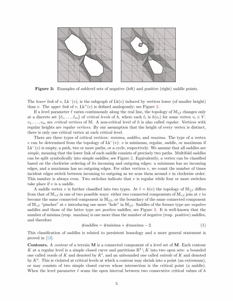
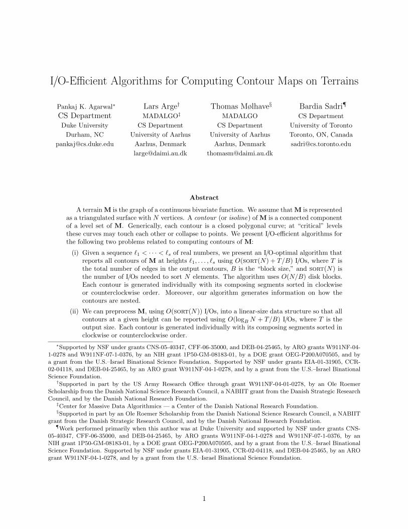
Figure 3: Examples of sublevel sets of negative (left) and positive (right) saddle points.

The lower link of v, Lk−(v), is the subgraph of Lk(v) induced by vertices lower (of smaller height)than v. The upper link of v, Lk+(v) is defined analogously; see Figure 2.

If a level parameter ` varies continuously along the real line, the topology of M≤` changes onlyat a discrete set {`1, . . . , `m} of critical levels of h, where each `i is h(vi) for some vertex vi ∈ V .v1, . . . , vm are critical vertices of M. A non-critical level of h is also called regular. Vertices withregular heights are regular vertices. By our assumption that the height of every vertex is distinct,there is only one critical vertex at each critical level.

There are three types of critical vertices: minima, saddles, and maxima. The type of a vertexv can be determined from the topology of Lk−(v): v is minimum, regular, saddle, or maximum ifLk−(v) is empty, a path, two or more paths, or a cycle, respectively. We assume that all saddles aresimple, meaning that the lower link of each saddle consists of precisely two paths. Multifold saddlescan be split symbolically into simple saddles; see Figure 2. Equivalently, a vertex can be classifiedbased on the clockwise ordering of its incoming and outgoing edges: a minimum has no incomingedges, and a maximum has no outgoing edges. For other vertices v, we count the number of timesincident edges switch between incoming to outgoing as we scan them around v in clockwise order.This number is always even. Two switches indicate that v is regular while four or more switchestake place if v is a saddle.

A saddle vertex v is further classified into two types. At ` = h(v) the topology of M≤` differsfrom that of M<` in one of two possible ways: either two connected components of M<` join at v tobecome the same connected component in M≤`, or the boundary of the same connected componentof M<` “pinches” at v introducing one more “hole” in M≤`. Saddles of the former type are negativesaddles and those of the latter type are positive saddles; see Figure 3. It is well-known that thenumber of minima (resp. maxima) is one more than the number of negative (resp. positive) saddles,and therefore

#saddles = #minima + #maxima− 2. (1)

This classification of saddles is related to persistent homology and a more general statement isproved in [13].

Contours. A contour of a terrain M is a connected component of a level set of M. Each contourK at a regular level is a simple closed curve and partitions R2 \K into two open sets: a boundedone called inside of K and denoted by K i, and an unbounded one called outside of K and denotedby Ko. This is violated at critical levels at which a contour may shrink into a point (an extremum),or may consists of two simple closed curves whose intersection is the critical point (a saddle).When the level parameter ` scans the open interval between two consecutive critical values of h

5

Figure 4: Red and blue contours in a level-set of a terrain.

the contours of M` change continuously and the topology of M` remains unchanged. However, at acritical level the contours that contain the corresponding critical point undergo topological changes.Let K1 and K2 be two contours at levels `1 and `2 respectively with `1 < `2. We regard K1 and K2

as “the same” if K1 continuously deforms into K2 (without any topological changes), as z` sweepsM in the interval [`1, `2].

Following [1], we call a contour K in M` blue if, “locally”, M<` lies in K i, and red otherwise; seeFigure 4. Every blue contour is born as a single point at a minimum. Conversely, a blue contour isborn at every minimum except at v∞. Because of being placed at infinity, a red contour is born atv∞. Likewise, a red contours “dies” by shrinking into a single point at a maximum, and conversely,some red contour dies at every maximum. Two contours, with at least one of them being blue,merge into the same contour at a negative saddle. The resulting contour is red if one of the mergingcontours is red, and blue otherwise. A contour splits into two contours at a positive saddle. A redcontour splits into two red contours while a blue contour splits into one red and one blue contour.

Two contours Ki and Kj of a level set M` are called neighbors if no other contour K of M`

separates them, i.e., one of Ki and Kj is contained in K i and the other in Ko. If Ki is neighborto Kj and Ki ⊂ K i

j , then Ki is called a child of Kj . If Ki ⊂ Koj and Kj ⊂ Ko

i then Ki is called asiblings of Kj . It can be verified that all children of a red (resp. blue) contour are blue (resp. red)contours while all siblings of a red (resp. blue) contour are red (resp. blue) contours.

We conclude this section by making a key observation, which is crucial for our main result.Each regular contour of M corresponds to a cycle in M∗: let K be a contour in an arbitrary levelset M`, and let F (K) (resp. E(K)) denote the set of faces (resp. edges) of M that intersect K.If K is a red (resp. blue) contour, all the edges in E(K) are oriented toward K i (resp. Ko).Consequently, the vertices in F ∗(K) are linked by the edges in E∗(K) into a cycle in M∗. We referto this cycle as the representing cycle of K. We use C(K,M) to denote the circular sequence oftriangles dual to the representing cycle of K in M. The sequence in C(K,M) is oriented clockwise(resp. counterclockwise) if K is blue (resp. red); see Figure 5.

6

(a) (b)

Figure 5: (a) Orientation of the edges in the plane triangulation M of a terrain. Critical pointsand a contour K in a regular level set are shown. (b) the dual M∗ of M. The representing cycle ofK in M∗ is shown with bold edges. Triangles in C(K,M) are shaded.

3 Level-ordering of Triangles

In this section we present our main result, i.e. the existence of a level-ordering on triangles ofany terrain M, i.e., an ordering that satisfies conditions (C1) and (C2). We begin by proving theexistence of a level-ordering for terrains that do not have saddle vertices. We call such terrainsbasic. Next we prove certain structural properties of terrains and show that any arbitrary terraincan be transformed into a basic terrain through a surgery that effectively “preserves” the contoursof the original terrain. We then argue that a level-ordering on the transformed terrain correspondsto a level-ordering on the original one.

3.1 Basic terrain

Let M be a basic terrain. The above discussion and (1) imply that M has one (global) minimum,v, which coincides with v∞, and one (global) maximum, v, and that every level set consists of asingle red contour. At v this contour collapses into a single point.

Lemma 3.1 Let P ⊂ E be a directed (monotone) path in M from v to v. Then every cycle of M∗contains exactly one edge from P ∗. In particular, the graph M∗ \ P ∗ obtained from deleting theedges in P ∗ from M∗ is acyclic.

Proof. We claim that v is reachable in M from every vertex v ∈ V . Recall that v is the onlylocal maximum in M and that every other vertex has at least one outgoing edge. If one starts atv and follows an arbitrary outgoing edge at each step, the height of the vertex at which we arriveis greater than that of the previous one. This process can only stop at v. By a similar argument,every vertex v ∈ V is reachable from v.

Consider an arbitrary cycle C∗ in M∗. In the plane drawing of M∗, C∗ is a Jordan curve. LetV0 ⊂ V be the set of vertices that are contained in the inside of C∗ (equivalently, V ∗0 ⊂ V ∗ is theset of faces of M∗ whose union is bounded by C∗). Let C ⊂ E be the set of edges in M dual tothose in C∗. Since C∗ is a cycle, the edges in C are either all oriented from V0 to V \V0 or all fromV \ V0 to V0.

The former case cannot happen because v∞ 6∈ V0 and every vertex in V is reachable from v∞. Ifall edges of C are oriented from V \ V0 to V0, then v ∈ V0 because otherwise v cannot be reachable

7

from the vertices of V0. Since v ∈ V0 and v∞ ∈ V \ V0, |P ∩C| ≥ 1. There is no edge directed fromV0 to V \ V0, so once P reaches a vertex of V0 it cannot leave V0, implying that |P ∩C| = 1. Thus,every cycle of M∗ is destroyed by the removal of the edges in P ∗, implying that M∗ \ P ∗ is acyclic.�

Let P be the path from v to v as defined in Lemma 3.1. The graph M∗ \ P ∗ has all of thevertices of M∗. Thus every face f of M is represented by f∗ in M∗ \ P ∗. Let ≺ be the a binaryrelation on F (triangles in M) defined as f1 ≺ f2 if (f∗1 , f

∗2 ) ∈ E∗ \P ∗. Since by Lemma 3.1 M∗ \P ∗

is acyclic, ≺ is a partial order on F . We call ≺ the adjacency partial order induced by the acyclicgraph M∗ \ P ∗. A linear extension of ≺ is any total order / on F that is consistent with ≺, i.e.f1 ≺ f2 implies f1 / f2. Such a linear extension can be obtained by topological sorting of M∗ \ P ∗.By definition, the existence of a directed path from f∗i to f∗j in M∗ \ P ∗ implies that fi / fj . Thuscondition (C1) of the definition of level ordering holds for /. Since in a basic terrain each levelconsists of only one contour, condition (C2) holds trivially. This results the following statement.

Corollary 3.2 Let M be a basic terrain, and let P be a directed (monotone) path from v to vin M. Let / be a linear extension of the adjacency partial order induced by M∗ \ P ∗. Then / is alevel-ordering of the triangles of M.

3.2 Red and blue cut-trees

Consider now a non-basic terrain with saddle vertices. We first introduce the notions of ascending(red) and descending (blue) cut-trees of M as subgraphs of the triangulation M, which we lateruse to turn M into a basic terrain M. Contours of each level set of M will then be encoded in acorresponding level set of M which consists of a single contour.

A descending (resp. ascending) path on M from a vertex v ∈ V is a path v0, v1, . . . , vr wherev0 = v and h(vi) < h(vi−1) (resp. h(vi) > h(vi−1)) for i = 1, . . . , r. For each negative saddle v, letP1(v) = u0, u1, . . . , ur and P2(v) = w0, . . . , ws be two descending paths from v such that ur and wsare both minima and u1 and w1 belong to different connected components of Lk−(v). Furthermoreassume that for any two negative saddles u and w, if Pi(u) = u0, . . . , ur and Pj(w) = w0, . . . , ws,for some i, j ∈ {1, 2}, and uk = wl for some 1 ≤ k ≤ r and 1 ≤ l ≤ s, then uk+1 = wl+1; in otherwords, descending paths from different vertices can join but then cannot diverge. Such a set ofpaths always exist: one can assign such paths to negative saddles in the increasing order of theirheights. At any negative saddle u, we follow a descending paths through each of the two connectedcomponents of Lk−(u) until it either reaches a minimum or joins a path already assigned to alower negative saddle. Let P (u) = P1(u) ∪ P2(u) for any negative saddle u. Since P1(u) \ {u} andP2(u) \ {u} are contained in different connected components of M<h(u), the underlying undirectedgraph of P (u) is a simple path. For a positive saddle u, P1(u) and P2(u) are defined similarly usingascending paths that start at different connected components of Lk+(u) and end in maxima.

We define the descending (blue) cut-tree T = (V , E) of M to be the union of the paths P (u)over all negative saddles u. Similarly, we define the ascending (red) cut-tree T = (V , E) of M to bethe union of all the paths P (u) over all positive saddles u. It is, of course, not clear that T and Tare trees but this and some of their other properties are proven below.Remark. The definitions of red and blue cut-trees are closely related to the notions of split andjoin trees in the context of contour trees [21]. Intuitively the contour tree is the result of contractingeach contour of M into a single point 1 and is topologically a connected collection of simple curves

1Taking the terrain M as a topological space with the usual topology of R2 and defining an equivalence relation∼ between points on M as x ∼ y if and only if x and y are on the same contour (connected component of some levelset), the contour tree M∼ of M is the quotient space of M modulo ∼.

8

uvx

y

v

v

u v

xy

v

v

Figure 6: A terrain for which the join tree cannot be embedded as a subgraph of the underlyingtriangulation in such a way that the edges are realized by ascending paths. Level sets of saddles aredepicted in dotted lines. The contour tree of the terrain on the left is shown on the right. Noticethat there is no directed (ascending) path from x to y on the terrain.

whose endpoints correspond to the critical points of M. These curves can only intersect at theirendpoints and thus realize the edges of a graph on a set of vertices that correspond to the criticalpoints of M. It can be shown that this graph is always connected and acyclic — hence the namecontour tree.2 Each point on a curve realizing an edge represents a contour at some height. Theheights of points along any edge of the contour tree vary monotonically from one end to the other.The contour tree is often described as the union of two of its subtrees, namely the merge and splittrees. The join tree is the minimal connected subtree of the contour tree that contains minima andnegative saddles and the split tree is defined analogously using maxima and positive saddles.

The similarity between the notions of blue (resp. red) cut-tree and join (resp. split) tree natu-rally poses the question of whether our cut-trees can be replaced by their contour tree counterparts.We emphasize here that our cut-trees are subgraphs of the triangulation M and this plays a crucialrole in our algorithms. It is possible to draw the contour tree on the terrain in such a way that thevertices coincide with their corresponding critical points and edges are realized by monotonicallyascending curves on the terrain. It is easy to observe that if one can realize each edge of the joinor split tree as a monotonically ascending path in M then it is indeed possible to simply use themerge or split trees in place of our cut-trees. However, this is not always possible as the terraindepicted in Figure 6 demonstrates.

Lemma 3.3 The underlying undirected graph of a blue (resp. red) cut-tree T (resp. T) has nocycles.

Proof. We prove the claims for blue cut-tree. The argument for red cut-tree can be made symmet-rically. Let u1, . . . , ur be the list of all negative saddles of M in the increasing order of their heights.Let T0 be the empty graph and for each i = 1, . . . , r, let Ti =

⋃ij=1 P (uj); Ti−1 is a subgraph of

Ti, and Tr = T. We prove by induction on i that the underlying undirected graph of each Ti isa forest. This trivially holds for T0. Assume now that the underlying undirected graph of Ti isa forest. By construction, adding P (ui+1) connects two distinct connected components of Ti, onecontained in each of the two distinct connected components of M<h(ui+1) that join at ui+1.

Moreover, once each of P1(ui+1) or P2(ui+1) reaches a vertex of Ti, it continues by following a

2Indeed such graphs, known generally as Reeb graphs [22], can be obtained from arbitrary continuous real valuedfunctions defined on more general topological spaces such as arbitrary manifolds. Contour trees are Reeb graphs ofterrains as determined by their height functions.

9

Figure 7: Cutting a triangulation along a tree.

path contained in Ti, and therefore does not introduce a cycle within the corresponding connectedcomponent of Ti. �

For a set U ⊆ R2, let T(U) (resp. T(U)) be the union of the paths P (u) for all negative (resp.positive) saddles u ∈ U . In particular, T = T(R2) and T = T(R2).

Lemma 3.4 For a blue (resp. red) contour K, the underlying undirected graph T(K i) (resp.T(Ko)) connects all of the minima in K i (resp. Ko). A symmetric statement holds regarding Tand maxima by switching “red” and “blue”.

Proof. We prove the lemma for T and blue contours. The other cases are similar. Let K be ablue contour in Mλ for some λ ∈ R. We show that for each ` ∈ R, the minima in each connectedcomponent of U` = M<` ∩K i are connected by T(U`). The statement of the lemma then followsby taking ` to be larger than the height of all vertices in K i and from the fact that in that case U`consists of a single component.

To prove the lemma we sweep ` from −∞ toward +∞ and verify the claim for U`. Every time` reaches the height of a minimum in K i, a new connected component is added to U`. The lemmaholds for this new component since it originally has only a single minimum which is vacuouslyconnected by T(U`) to every other minimum in that component. The validity of the claim as `continues to raise can only be altered when ` reaches the height of a negative saddle u in K i atwhich two connected components U1 and U2 of U<`, where ` = h(u), join at u. At this time thepath P (u) is added to T(U`). The crucial observation here is that because K is a blue contour, nodescending path started at a vertex u ∈ K i can reach Ko. Thus the endpoints of P (u) have to beminima in K i. In other words P (u), which reaches a minimum in U1 and another in U2, connectsT(U1) and T(U2) as desired. �

Corollary 3.5 The underlying undirected graphs of T and T are trees. Moreover, all minima arevertices of T and all maxima are vertices of T.

We conclude this discussion by mentioning a property of T and T that follows from theirconstructions.

Lemma 3.6 Let u be a vertex of T (resp. T). If u is a positive (resp. negative) saddle, then uhas two outgoing (resp. incoming) edges in T (resp. T) — one to each connected component ofthe upper (resp. lower) link of u in M. If u is a regular vertex or a negative saddle, then u hasone outgoing (resp. incoming) edge. Finally, if u is a maximum (resp. minimum), then it has nooutgoing (resp. incoming) edges.

3.3 Surgery on terrain

Let T be a red cut-tree for M. Consider the following combinatorial operation on M. First weduplicate every edge e of T, thus creating a face fe that is bounded by the two copies of e. We then

10

(a) (b) (c)

Figure 8: (a) A red (ascending) cut-tree marked T marked on the terrain M of Figure 5. (b)Construction of the graph M0: the terrain is cut along T and a new maximum v is inserted in theopened face. On the right, a blue cut-tree of M0 is marked. (c) Construction of the graph M: theterrain is cut open on the red cut-tree and a new maximum is inserted.

perform an Eulerian tour on the subgraph of M induced by the copies of the edges of T in whichat each vertex the next edge of the tour is the first unvisited edge of the subgraph in clockwiseorder, relative to the previous edge of the tour. We then combine all of the faces fe into a singleface f that is bounded by this Eulerian tour by making as many copies of each vertex as its degreein T (or equivalently the number of times the tour has passed through it) and connecting non-treeedges incident on u to appropriate copies of u; see Figure 7. Geometrically, the above modificationof the terrain triangulation can be interpreted as “puncturing” the plane along the edges of T andintroducing a new face f bounded by the 2|E| edges in the Euler tour.

We then subdivide f by placing a new vertex v inside it and connecting v via incoming edges(u, v) to every vertex u on the boundary of f . The result is a triangulation M0 = (V0, E0, F0); seeFigures 8 (a) and (b). The newly added triangles are all incident to v, and we refer to them asv-triangles. The edge e opposite to v in a v-triangle f (which is a copy of a T edge) is called thebase of f and f is said to be based at e. One can modify the plane drawing of M into a (singular)plane drawing of M0, that has faces of zero area and edges that bend and overlap, by jamming allthe new faces and edges in the (zero-area) hole that results from cutting the plane along T.

M0 can be regarded as the triangulation of a terrain M0: Fary’s theorem [14] can be used tostraight-line embed M0 while preserving all its faces and the height function of M induces a heightfunction on triangles of M0 that are also in M. The height of v is then chosen to be higher thanthe heights of all vertices of M and is used to linearly interpolate a height function on v-triangles.

Lemma 3.7 M0 has no positive saddles and exactly one maximum, namely v. The minima of M0

are precisely those of M. Each negative saddle of M0 is a copy of a negative saddle of M, and onlyone copy of each negative saddle of M is a negative saddle of M0.

Proof. For a vertex u 6∈ T, Lk(u) is the same in M and M0 modulo taking copies of T vertices asidentical. In particular, minima of M stay minima in M0. Thus it suffices to consider v and copiesof T vertices. Clearly, v is a maximum. Let u be a vertex of T, and let u′ be a copy of u in M0.Let e′1 and e′2 be copies of T edges that enter and leave u′, respectively, in the Eulerian tour of T.Both of these edges remain incident to u′ in M0. Let v′1 and v′2 be other endpoints of e′1 and e′2 inM0, respectively. Let vi and ei, i = 1, 2, be the vertex and edge in M corresponding to v′i and e′i,respectively. Lk(u′) consists of a path π(u′) from v′1 to v′2 followed by v. Moreover, e′1 and e′2 arethe only edges incident on u′ that are copies of T edges, and π(u′) is also a path in Lk(u) in M,

11

modulo taking copies of T vertices as identical.First, u′ cannot be a maximum because u′ is adjacent to v. It cannot be a minimum either

because then π(u′) ⊆ Lk+(u) and e1 and e2 are outgoing edges from u in T connected to somecomponent of Lk+(u), which contradicts Lemma 3.6. Next, if Lk+(u′) is not connected, then itscomponent U not containing v does not contain v′1 and v′2 either and thus u lies in the interior ofthe path π(u′). Then U is also a connected component of Lk+(u) in M. Unless u is a negativesaddle, by Lemma 3.6, there is an outgoing edge in T from u to a vertex in U , contradicting thefact that e′1 and e′2 are the only edges adjacent to u′ that are copies of T edges. Hence, unless u isa negative saddle, Lk+(u′) is connected and u′ is a regular vertex in M0.

Finally, suppose u is a negative saddle, with two components U1 and U2 in Lk+(u). By Lemma3.6, u has exactly one outgoing edge e in T. Without loss of generality assume that e is connectedto U1. Then U2 will appear as a connected component of the upper link of exactly one copy u′ of u,namely if U ⊆ π(u′), and u′ will be a negative saddle in M0. The upper link of all other copies of uwill be connected — consisting of v and possibly a portion of U1. Consequently, one copy of everynegative saddle of M becomes a negative saddle in M0 and other copies become regular vertices.This completes the proof of the lemma. �

Next we perform a similar surgery on M0 only using a blue cut-tree T of M0. As above, theidea is to slice the plane along T and insert a new vertex v in the resulting face and connect vto every copy u of a vertex in T by an outgoing edge (v, u). We call the resulting triangulationM = (V , E, F ). A slight technicality arises in this case as a result of the fact that v∞ is a minimumof M0 which by Corollary 3.5 is a vertex of T. As it will become clear later, we only need to treatv symbolically below v∞ by connecting them by an edge oriented toward v∞. We conclude, usingthe same argument as in Lemma 3.7, the following:

Lemma 3.8 M does not have saddle vertices.

Lemma 3.9 If (f∗1 , f∗2 ) is an edge of M∗, then there is a path from f∗1 to f∗2 in M∗.

Proof. If f1 and f2 are adjacent in M then (f∗1 , f∗2 ) is an edge in M∗. Thus we only need to consider

the case in which an edge e shared by f1 and f2 in M is an edge of T or T (or both). Suppose e is anedge of T. In constructing M0, e is duplicated to create two edges e1 and e2, respectively, incidentto f1 and f2. Let φ1 and φ2 respectively be the v-triangles based at e1 and e2. By construction, f1is to the left and φ1 to the right of e1 and therefore (f∗1 , φ

∗1) is an edge in M∗. Similarly (φ∗2, f

∗2 ) are

edges in M∗. Consider the subgraph of M∗ induced by v-triangles. Since all the edges incident to vare incoming, their duals make a cycle in M∗ which includes φ∗1 and φ∗2. Since there is a path fromφ∗1 to φ∗2 on this cycle and there are edges from f∗1 to φ∗1 and from φ∗2 to f∗2 in M∗, we get a pathfrom f∗1 to f∗2 . It is easy to observe that the same argument extends to neighboring M trianglesthat are separated by the edges of T or both T and T. �

3.4 Encoding of contours in the resulting basic terrain

Although we argued above that M can be realized and therefore treated as the triangulation of aterrain M, to relate the level sets of M to those of M, in the rest of this section we use a degeneraterealization of M as a surface in R3 that differs from what a straight-line embedding of M results.This substantially simplifies the arguments that follow. We shall realize the v- and v-triangles asvertical curtains: An upward (resp. downward) extending curtain based at a segment pq in R3 isthe convex hull of two infinite rays shot in positive (resp. negative) direction of the z-axis from thepoints p and q respectively. A curtain can be regarded as a vertical (orthogonal to the xy-plane)triangle that has a vertex at infinity.

12

Figure 9: Left: The red cut-tree T of a terrain is drawn using heavier segments on the terrainM. Middle: The terrain is sliced along T and v-triangles are represented by upward extendingcurtains. Note that each edge e of T results two overlapping curtains one based at each of the two(overlapping) copies of e that results from cutting the terrain along T. Right: A contour of theresulting terrain (dashed) overlapping itself on v-triangles.

We realize M by preserving the geometry of every triangles that existed in M and representingv-triangles (resp. v-triangles) as upward (resp. downward) extending curtains based at segmentscorresponding to the edges of T (resp. T) on M; see Figure 9. Note that in this realization ofM, the two copies of each T or T edge overlap as do the segments that represent them on M andtherefore the curtains tha realize their corresponding v- or v-triangles also overlap. Although inthis sense M is not the graph of a bivariate function, it can still be regarded as a (self-overlapping)piece-wise linear surface in R3 and a level set M` of it can be defined as the projection into thexy-plane of the set M` = M ∩ z`. Let T and T respectively be shorthands for M(T) and M(T).Note that T and T are also contained in M, although under the topology of this surface they are(self-overlapping) closed curves that correspond to Eulerian traversals of T and T on M.

Since every triangle of M is also in M and is geometrically realized by the same triangle in bothM and M, M` ⊆ M` for all ` ∈ R and M` \M` ⊂ T ∪ T (with some abuse of notation we write Tand T to refer the red and blue cut-trees as subgraphs M as well as their drawings as subsets ofR2). In other words M` consists of the contours of M` together with fragments of the red and bluecut-trees.

Lemma 3.10 Let K0 be a blue (resp. red) contour in a level set M` and let K1, . . . ,Kr be itschildren. Let R be the interior of K i

0 \ (K i1 ∪ · · · ∪K i

r). Then M` ∩R = T ∩R (resp. T ∩R).

Proof. We prove the lemma for the case where K0 is blue. The proof for the case where it is red issymmetric. Let Q and Q respectively be shorthands for M(R) and M(R). By definition, Q ⊆ Q.Since K0 is a blue contour of M, Q is entirely below the plane z`. Since Q and Q differ only incurtains based at T or T segments, z` ∩ Q is contained in such curtains. On the other hand anycurtain whose intersection with Q intersects z` has to be extending upward from some segment ofT that intersects Q. Thus M` ∩R ⊆ T. Conversely, any segment of T that intersects Q is the baseof an upward extending curtain which intersects z`. Thus T ∩R ⊆ M`. �

Let us fix a regular level ` of h and and let K1, . . . ,Kt be the contours in M`. For sim-plicity, we virtually add an infinitely large contour K0 that bounds the entire plane. Let K` ={K0,K1, . . . ,Kt}. Consider the set R` = {R0, R1, . . . , Rt} of the connected component of R2 \M`.The boundary of each Ri, i ≥ 0, consists of a set B(Ri) = {Ki0 ,Ki1 , . . . ,Kir(i)} ⊆ K` of r(i)contours in which Ki1 , . . . ,Kir(i) are the children of Ki0 in the arrangement of contours in K`.

For any R ∈ R` we construct an undirected graph G`(R) = (VR, ER) as follows. By Lemma3.10, M` ∩ R is contained in exactly one of T or T; let T denote that tree. The vertex set VR ofG`(R) consists of all the vertices of T that are contained in R together with one auxiliary vertexvK associated with every contour K ∈ B(R). The edge set ER of G`(R) consists of an edge {u, v}corresponding to each edges (u, v) of T whose endpoints u and v are both in R together with an edge

13

{v, vK} for any edge of T that crosses a contour K ∈ B(R) and its endpoint in R is v. Equivalently,G`(R) is obtained from the subgraph of T that is induced by those edges of T that intersect R, byidentifying all vertices that are contained in each component R′ 6= R of R` that is separated fromR by a contour K ∈ B(R) into a single vertex vK .

Lemma 3.11 For any R ∈ R` the graph G`(R) as defined above is a tree.

Proof. Let K0,K1, . . . ,Kr be the contours bounding R and let K0 be the parent of K1, . . . ,Kr. Weprove the lemma for the case where K0 is blue. The proof for the case where it is red is symmetric.We prove that the existence of a cycle in G`(R) implies the existence of a cycle in the underlyingundirected graph of T which contradicts Corollary 3.5. Consider any contour Kj , j ≥ 1 and let

e1 = (u1, v1) and e2 = (u2, v2) be two edges of T that intersect Kj . Since Kj is red, v1, v2 ∈ K ij .

Since e1 is an edge of T, v1 is followed in T by an ascending path that ends at a maximum. Sinceno ascending path can leave K i

j , T reaches a maximum v′1 in K ij through v1. Similarly, T reaches a

maximum v′2 in K ij through v2. Lemma 3.4 implies that v′1 and v′2 are connected by a path in the

underlying undirected graph of T that is contained in K ij . In other words, any two branches of T

that enter K ij meet in K i

j . Thus if we contract every edge of T whose endpoints are both outsideR, we precisely get the graph G`(R). The proof of the lemma follows from the fact that the resultof contracting a tree edge is a tree. �

We next combine the graphs G`(R), R ∈ R` into a graph G` by identifying, for any two com-ponents R1 and R2 that share a contour K in their boundaries, the two auxiliary vertices vKassociated to K in G`(R1) and G`(R2). The acyclic structure of the hierarchy of red and bluecontours together with Lemma 3.11 result the following statement.

Corollary 3.12 The graph G` is a tree.

Let P be a v-v path in M. Since M is a basic terrain (does not have saddle vertices), byLemma 3.1 M∗ \ P ∗ is acyclic. Let ≺ be the adjacency partial order on F induced by M∗ \ P ∗.Since F ⊂ F , ≺ is also a partial order when restricted to F .

Lemma 3.13 Let / be a linear extension of ≺ on F . If K and K ′ are two contours of a level setM` and f1, f2 ∈ F (K) and f ′1, f

′2 ∈ F (K ′) are such that f1 / f

′1 / f2, then f1 / f

′2 / f2.

Proof. Since M is a basic terrain, M` consists of a single contour. Let C∗ = C(K,M∗) be therepresenting cycle of M` in M∗. If f1, f2 ∈ F (K) for some contour K in M` and the edge commonto f1 and f2 does not belong to either of T or T, then (f∗1 , f

∗2 ) is an edge in C∗. By Lemma 3.1,

C∗ has exactly one edge in P ∗. Thus C∗ \ P ∗ is a path Q∗ that is exactly one edge short of C∗.Let G` be the tree of Corollary 3.12. We map the path Q∗ in M` into a walk W in G` as follows:

Each vertex f∗ of Q∗ is mapped to a pair (u, v) where either u and v are neighboring vertices inG` or u = v. Specifically, if f ∈ M`(K), then f∗ is mapped into (vK , vK) where vK is the vertexof G` that represents K. Otherwise, f∗ is dual to of some v- or v-triangle f in M that intersectsM`. Let e = (u, v) be the edge in M at (a copy of) which f is based in M. If the edge e does notintersect M`, it is contained in G`(R) (as an undirected edge) for precisely one R ∈ R`, in whichcase we map f∗ to (u, v). On the other hand, if e intersects M` at a contour K, then by Lemma3.10 there will be precisely one edge {vK , v} in G` where v is an endpoint of e, in which case wemap f∗ into (v, vK). It can be verified that the set of pairs in the image of Q∗ under this mappingis indeed a walk W in G`. Since M` goes thorough any segment s at most twice, each edge of G`appears at most twice in W .

14

Figure 10: Contours of M` (left) versus those of M` (right).

For f1 / f′1 / f2 to hold, Q∗ must visit f∗1 , f ′1

∗ and f∗2 in this order. Assume without loss ofgenerality that f ′1 / f

′2. In order for f1 / f

′2 / f2 not to hold, one must have f2 / f

′2 which means Q∗

must visit f ′2∗ after f∗2 . But this corresponds to going from K to K ′, then back to K and then again

to K ′. Since each of K and K ′ are represented by a vertex in G` this would mean that W goesthorugh vK , vK′ , and again vK in this order. Corollary 3.12 implies then that W has to traversesome edge of G` at least three times, a contradiction. �

Lemmas 3.9 and 3.13 respectively prove that the total order / has properties (C1) and (C2) ofa level-ordering .

Theorem 3.14 For any terrain M with triangulation M, there is exists a level level-ordering ofthe triangles of M.

4 Contour Algorithms

In this section we describe I/O-efficient algorithms for computing contour maps as well as an I/O-efficient data structure for answering contour queries.

4.1 Level-ordering of terrain triangles

We describe an I/O-efficient algorithm for computing, given a terrain M, the triangulation M ofthe simplified terrain M, and a monotone path P from v to v in M. We can then compute alevel-ordering of the triangles of M in O(sort(N)) I/Os using an existing I/O-efficient topologicalsorting algorithm for planar DAGs [8]. This induces a level-ordering on the triangles of M.

Computing the red cut-tree. The first step in computing M is to compute a red (ascending)cut-tree T of M. The I/O-efficient topological persistence algorithm of Agarwal et al. [2] candetermine the type (regular, minimum, negative saddle, . . . ) of every vertex of M in O(sort(N))I/Os. Moreover, for every vertex v ∈M, it can also compute, within the same I/O bound, a vertexfrom each connected component of Lk+(v). Since each saddle of M is assumed to be simple, Lk+(v)has at most two connected components.

To compute T, we apply the time-forward processing technique [10] using a priority queue Q:we scan the vertices of M in the increasing order of their heights. We store a subset of vertices inQ, namely the upper endpoints of the edges of T whose lower endpoints have been scanned. Thepriority of a vertex v in Q is its height h(v). Suppose we are scanning a vertex v of M and u isthe lowest priority vertex in Q. If h(v) < h(u) and v is not a positive saddle, we move to a new

15

vertex in M. Otherwise, i.e. if h(u) = h(v) or v is a positive saddle, we choose a vertex w fromeach connected component of Lk+(v), which we have already computed in the preprocessing step.We add the edge (v, w) to T and add w to Q. Since each operation on Q can be performed in

O(

1B logM/B N/B

)I/Os, T can be computed in O(sort(N)) I/Os.

Adding the blue cut-tree. The second step in computing M is to compute a blue cut-tree T ofM0. However, we can compute T directly on M if we ensure that T and T do not cross each other,even though they can share edges. This property can be ensured by choosing the ascending anddescending edges, in T and T, respectively, out of each vertex v, more carefully. Specifically, weuse the following rule:

1. On an ascending path, the edge following (u, v) is (v, w) where (v, w) is the first outgoingedge out of v after (u, v) in clockwise order, and

2. On a descending path, the edge following (v, u) is (w, v) where (w, v) is the first incomingedge of v after (v, u) in counterclockwise order.

It can be verified that T and T do not cross. One can therefore compute T precisely in the sameway as T directly on M.

Computing a monotone v-v path P . While computing T we also compute a descending pathstarting at the lowest positive saddle v1 of M as though v1 were another negative saddle. This pathP , which ends at a T vertex v0, together with (v, v0) and (v1, v) serves as a monotone path in Mconnecting v to v.

Generating M∗ \ P ∗. The topological sorting algorithm of Arge et al. [8] takes as input a planardirected acyclic graph, represented as a list of vertices along with the list of edges incident uponeach vertex in circular order. Given M, T, T, and P , we need to compute such a representationof M∗ \ P ∗. Since each face in M is a triangle, M∗ is 3-regular. It is easy to compute the circularorder of edges incident upon a vertex of M∗ whose dual triangle is neither a v- or v-triangle, noradjacent to a copy of a T or T edge. The main task is then to compute these the v- and v-triangles.This can be accomplished by computing the Eulerian tours of T and T, which takes O(sort(N))I/Os [8]. Putting everything together, we obtain the main result of this paper.

Theorem 4.1 Given a terrain M with triangulation M, a level-ordering of the triangles of M canbe computed in O(sort(N)) I/Os, where N is the number of vertices of M.

4.2 Contour maps of basic terrains

Let L = {`1, . . . , `s} be a set of input levels with `1 < · · · < `s. Given a basic terrain M, the goal isto compute the contour map of M for levels in L. Since M is simple, each M`i consists of a singlecontour. Generating the segments of M`i in clockwise or counterclockwise order is equivalent tolisting the triangles of M that the contour M`i intersects in that order, i.e. reporting C(M`,M).

Our algorithm uses a buffer tree B to store the triangles of M that intersect a level set. Thebuffer tree [5] is a variant of B-tree, which propagates updates from the root to the leaves in alazy manner, using buffers attached to the internal nodes of the tree. As a result, a sequence of Nupdates (inserts and deletes) can be performed in amortized O(sort(N)) I/Os. Moreover, one canperform a flush operation on a buffer tree that results in the writing of all its stored elements onthe disk in sorted order. Flushing a tree with T elements takes O(T/B) I/Os.

It is more intuitive to describe the algorithm as a plane sweep of M in R3. At the first step, thealgorithm computes a level-ordering / of the terrain triangles using Corollary 3.2. Then starting

16

at ` = −∞, the algorithm sweeps a horizontal plane z` in the positive z-direction. A target level `∗is initially set to `1. At any time the algorithm maintains the list of triangles of M that intersectthe sweeping plane in a buffer tree B ordered by /. Whenever the sweep plane encounters thebottom-most vertex of a triangle f , we insert f into B; f is deleted again from B when the planereaches the top-most vertex of f . When the sweep plane z` reaches the target level `∗ (or ratherthe lowest vertex of height `∗ or more when the sweeping is implemented discretely), we flush thebuffer tree. The generated list of triangles (vertices of M∗) are precisely the set of triangles in Mthat intersect z`∗ ordered by /. Corollary 3.2 implies that the output is exactly C(M`∗ ,M). Thealgorithm then raises the target level `∗ to the next level in L and continues.

Level-ordering of the terrain triangles takes O(sort(N)) I/Os (Theorem 4.1). Preprocessingfor the sweep algorithm consists of sorting the vertices in their increasing order of heights whichcan also be done in O(sort(N)) I/Os. During the sweep each update on the buffer tree takesO( 1

B logM/B N/B) amortized I/Os [5]. Thus all the O(N) updates can be performed in O(sort(N))I/Os in total. Each flushing operation takes O(T ′/B) I/Os, where T ′ is the number of trianglesin B. If a triangle is in B but has been deleted, it is not in B after the flushing operation, so a“spurious” triangle is flushed only once.

Hence, the total number of I/Os is O(sort(N) + T/B), where T is the output size. Finally, inaddition to storage used for the terrain the algorithm uses O(N/B) blocks to store the buffer treeand thus uses O(N/B) blocks in total.

4.3 Generalization to arbitrary terrains

Given a general terrain M with saddles, one can still compute by Theorem 4.1 a level-ordering ofthe triangles of M in O(sort(N)) I/Os. If one runs the algorithm of the previous section on M theoutput generated for each input level `i is C(M`i , M). Running the algorithm on M is equivalentto running it on M but ignoring all v and v-triangles by omitting their insertions into the buffertree. Consequently, the produced output for level `i is the same sequence of triangles only with vand v-triangles omitted. By Theorem 3.14 this is a subsequence R = 〈f1, . . . , fk〉 of C(M`i , M))in which C(K,M) of each contour K in M`i appears as a subsequence RK . Thus all one needsto do is to extract the subsequence RK and write it separately in the same order as it appears inR. Property (C2) of a level-ordering allows this to be done in O(k/B) I/Os: if in scanning thesequence R from left to right some elements of RK are later followed by elements of RK′ , then theappearance of another element of RK , indicates that no more elements from RK′ remain.

We thus scan the sequence R from left to right and push the scanned triangles into a stack SF .Every time the last element of a contour is pushed into the stack, the triangles of that contour makea suffix of the list of elements stored in SF . At such a point, we pop all the elements correspondingto the completed contour and write them to the disk. To find out when a contour is completed andhow many elements on the top of stack belong to it, we keep a second stack SE of edges. For anytriangle f ∈ F (M`i), two of the edges of f intersect M`i . With respect to the orientation of theseedges, f is to the right of one of them and to the left of the other one which we respectively callthe left and right edges of f at level `i. If e∗ = (f∗j , f

∗j+1) is an edge of the representing cycle of

a contour in M`i , then e is the right edge of fj and left edge fj+1 at level `i. We therefore checkwhen scanning a triangle fj whether its left edge is the same as the right edge of the triangle ontop of SF and insert fj into SF if this is the case. Otherwise, we compare the left edge of fj withthe edge on top of SE . If they are not the same, we are visiting a new contour and we insert theleft edge of fj into SE and fj into SF . Otherwise, fj is the last triangle of its contour. Thereforewe write it to the disk and successively pop and write to disk enough triangles from SF until theleft edge of a popped triangle matches the right edge of fj . We also pop this edge from SE . In

17

this algorithm each scanned triangle is pushed to the stack once and popped once. In a standardI/O-efficient stack implementation this costs O(k/B) I/Os.

Theorem 4.2 Given any terrain M with N vertices and a list L = {`1, . . . , `s} of levels with`1 < · · · < `s, one can compute using O(sort(N) + T/B) I/Os the contour map of M for levels inL, where T is the total number of produced segments.

4.4 Extracting nesting of contours

In addition to reporting each contour individually, a number of applications call for computinghow various contours are nested within each other. We produce this information by returning theparent of each contour in a computed contour map.

The parent-child relationship between individual contours in a contour map of a terrain M canbe read from the contour tree of M. Each contour in a contour map corresponds to a point onsome edge of the contour tree. Two contours K and K ′ in the map are neighbors (either siblingsor parent and child) if and only if their corresponding points on the contour tree can be connectedby a path that does not pass through a point corresponding to a third contour K ′′ 6= K,K ′ in thegiven contour map. Each edge of the contour tree can be colored red or blue according to the colorof the contours it represents (all contours represented by the points on the same edge of the contourtree have the same color). By the assumption that all saddles are simple, internal nodes of thecontour tree which correspond to saddles all have degree three. It can be verified that at a joining(negative) saddle only two color combinations on the edges incident to the saddles are possible.The same holds for a splitting (positive) saddle. In each case, using the edges colors, and usingthe corresponding patterns in which contours of various colors can merge or split, one can uniquelydetermine one of the edges incident to the saddle that carries contours that are parents to thosecarried by the other two. We “orient” this edge at each saddle away from and the other two towardthe saddle. The resulting orientation on the contour-tree is equivalent to orienting each blue edgetoward its higher end and each red edge toward its lower end. With this orientation of the contourtree a contour K will be the parent of a contour K ′, if the path between points representing K andK ′ on the contour tree follows the orientation of the edges of the tree.

The algorithm of Arge et al. [2] for computing the contour tree can return the color of each edgeon the generated tree. Thus if a contour tree of the terrain is available, by oriented the edges of thetree to point toward the neighboring edge and one can determine the edge of the contour tree onwhich each contour in a computed contour map is represented, one can determine the parent-childrelationship between individual contours in O(sort(N) + T/B) I/Os, where T is the number ofcontours in the given contour map, through a pre-order traversal of the oriented contour tree.

To facilitate finding of the edge the contour tree that carries a contour in the given map, insteadof the the contour tree, we compute the augmented contour-tree [2]. The augmented contour tree ofa terrain replaces each edge of the contour tree with a monotonically ascending path whose verticesare the vertices of the terrain. Every regular vertex of the terrain appears precisely once in one ofthese paths. All the properties of contour tree are also valid for the augmented contour tree. Westore in each vertex u of the terrain a pointer to each of the (at most two if u is a saddle and oneif u is regular) edges in the augmented contour tree that have u as the lower endpoint. To locatethe edge in the augmented contour tree corresponding to a computed contour K, we scan the listof triangles that intersect K and determine the vertices u and u′ of these triangles respectivelyhighest below and lowest above the level of K. Since there are no vertices between u and u′,shifting K down or up between h(u) and h(u′) does not change the set of triangles it intersectsand therefore its homology class. Consequently, uu′ is an edge of the augmented contour tree. All

18

that is needed then is to located the pointer to the contour tree edge stored at u that matches uu′.Since the augmented contour tree of a terrain of size N can be computed in O(sort(N)) I/Os [2],we summarize the above discussion as follows:

Theorem 4.3 For a contour map consisting of T contours of a terrain with N triangles, whereeach contour is given as a list of triangles that intersect it together with its level, one can reportfor each contour in the map a pointer to its parent in O(sort(N) + T/B) I/Os.

4.5 Answering contour queries

The sweep algorithm described in the previous section can easily be modified to construct a lin-ear space data structure that given a query level ` can report the contours in the level set M`

I/O-efficiently. Unlike the previously known structure for this problem [1], our structure can beconstructed in O(sort(N)) I/Os. To obtain the structure we simply replace the buffer tree B witha partially persistent B-tree [6, 23]. To build the structure, we sweep M by a horizontal plane inthe same way as we did in the algorithm of Section 4.2, inserting the triangles when the sweepplane reaches their bottom-most vertex, without checking for them to intersect any target levels,and deleting them when the sweep plane passes their top-most vertex. There will also be no needto flush the tree.

Since O(N) updates can be performed on a persistent B-tree in sort(N) I/Os [20, 7], thesweeping of the terrain require O(sort(N)) I/Os. A persistent B-tree allows us to query anyprevious version of the structure and in particular produce the list of the elements stored in thetree in O(logB N+T/B) I/Os when T is the number of reported elements. Therefore we can obtainM` in the same bound, simply by querying the structure for the triangles it contained when thesweep-plane was at height ` and then utilize Theorem 3.14 and the contour extraction algorithmdiscussed above to extract individual contours of M`.

Theorem 4.4 Given a terrain M with N vertices, one can construct in O(sort(N)) I/Os a linearsize data structure, such that given a query level `, one can report contours of M` in O(logB(N) +T/B)) I/Os where T is the size of the query output. Each contour is reported individually, and theedges of each contour are sorted in clockwise order.

5 Conclusions

We defined level-ordering of terrain triangles and proved that every terrain has a level ordering thatcan be computed I/O-efficiently. Based on this, we provided algorithms that compute contours ofa given terrain within similar I/O bounds. An immediate question is whether this approach canbe generalized to triangulated surfaces of arbitrary genus with arbitrary piecewise linear functionsdefined on them. Notice that the problem is valid even if the input surface is not embedded in R3.Another interesting open problem for surfaces that are embedded in R3 is computing of level setsor answering contour queries for a height function defined by a variable z direction: is it possible topreprocess a given triangulated surface embedded in the three space so that for any given direction,the contours of the height function for that direction can be computed I/O-efficiently?

19

References

[1] P. K. Agarwal, L. Arge, T. M. Murali, K. R. Varadarajan, and J. S. Vitter, I/O-efficient algo-rithms for contour-line extraction and planar graph blocking, Proc. 9th ACM-SIAM Sympos.Discrete Algorithms, 1998, pp. 117–126.

[2] P. K. Agarwal, L. Arge, and K. Yi, I/O-efficient batched union-find and its applications toterrain analysis, Proc. 22nd Annu. ACM Sympos. Comput. Geom., 2006, pp. 167–176.

[3] A. Aggarwal and J. S. Vitter, The input/output complexity of sorting and related problems,Commun. ACM, 31 (1988), 1116–1127.

[4] L. Arge, External memory data structures, in: Handbook of Massive Data Sets (J. Abello,P. M. Pardalos, and M. G. C. Resende, eds.), Kluwer Academic Publishers, 2002, pp. 313–358.

[5] L. Arge, The buffer tree: A technique for designing batched external data structures, Algo-rithmica, 37 (2003), 1–24.

[6] L. Arge, A. Danner, and S.-H. Teh, I/O-efficient point location using persistent B-trees, Proc.Workshop on Algorithm Engineering and Experimentation, 2003.

[7] L. Arge, K. H. Hinrichs, J. Vahrenhold, and J. S. Vitter, Efficient bulk operations on dynamicR-trees, Algorithmica, 33 (2002), 104–128.

[8] L. Arge, L. Toma, and N. Zeh, I/O-efficient topological sorting of planar dags, Proc. 15thAnnu. ACM Sympos. Parallel Algorithms and Architectures, 2003, pp. 85–93.

[9] H. Carr, J. Snoeyink, and U. Axen, Computing contour trees in all dimensions, ComputationalGeometry: Theory and Applications, 24 (2003), 75–94.

[10] Y.-J. Chiang, M. T. Goodrich, E. F. Grove, R. Tamassia, D. E. Vengroff, and J. S. Vitter,External-memory graph algorithms, Proc. 6th ACM-SIAM Sympos. Discrete Algorithms, 1995,pp. 139–149.

[11] Y.-J. Chiang and C. T. Silva, I/O optimal isosurface extraction, Proc. IEEE Visualization,1997, pp. 293–300.

[12] A. Danner, T. Mølhave, K. Yi, P. K. Agarwal, L. Arge, and H. Mitasova, TerraStream:From elevation data to watershed hierarchies, Proc. ACM Sympos. on Advances in GeographicInformation Systems, 2007, 212–219.

[13] H. Edelsbrunner, D. Letscher, and A. Zomorodian, Topological persistence and simplification,Discrete Comput. Geom., 28 (2002), pp. 511–533.

[14] I. Fary, On straight lines representation of planar graphs, Acta Sci. Math. Szeged, 11 (1948),229–233.

[15] M. Isenburg, Y. Liu, J. Shewchuk, and J. Snoeyink, Streaming computation of Delaunaytriangulations, Proc. of SIGGRAPH, 2006, pp. 1049–1056.

[16] W. Lorensen and H. Cline, Marching cubes: a high resolution 3d surface construction algo-rithm, Comput. Graph., 21 (1987), 163–170.

20

[17] M. H. Nodine, M. T. Goodrich, and J. S. Vitter, Blocking for external graph searching, Algo-rithmica, 16 (1996), 181–214.

[18] C. Silva, Y. Chiang, J. El-Sana, and P. Lindstrom, Out-of-core algorithms for scientific visu-alization and computer graphics, Visualization’02, 2002. Course Notes for Tutorial 4.

[19] R. A. Skelton, Cartography, History of Technology, 6 (1958), 612–614.

[20] J. van den Bercken, B. Seeger, and P. Widmayer, A generic approach to bulk loading multi-dimensional index structures, Proc. International Conference on Very Large Databases, 1997,pp. 406–415.

[21] M. van Kreveld, R. van Oostrum, C. Bajaj, V. Pascucci, and D. Schikore, Contour trees andsmall seed sets for isosurface traversal, Proc. 13th Annu. ACM Sympos. Comput. Geom., 1997,pp. 212–219.

[22] G. Reeb, Sur les points singuliers dune forme de Pfaff complement integrable ou dune fonctionnumerique. Comptes Rendus de LAcademie des Sciences, Paris 222 (1946), 847-849.

[23] P. J. Varman and R. M. Verma, An efficient multiversion access structure, IEEE Transactionson Knowledge and Data Engineering, 9 (1997), 391–409.

[24] J. S. Vitter, External memory algorithms and data structures: Dealing with MASSIVE data,ACM Computing Surveys, 33 (2001), 209–271.

21