ionolab-map: an automatic spatial interpolation algorithm...

Turk J Elec Eng & Comp Sci(2018) 26: 1933 – 1945© TÜBİTAKdoi:10.3906/elk-1611-231

Turkish Journal of Electrical Engineering & Computer Sciences

http :// journa l s . tub i tak .gov . t r/e lektr ik/

Research Article

IONOLAB-MAP: An automatic spatial interpolation algorithm for total electroncontent

Muhammet Necat DEVİREN1,2,∗, Feza ARIKAN2

1TÜBİTAK Defense Industries Research and Development Institute (SAGE), Mamak, Ankara, Turkey2Department of Electrical and Electronics Engineering, Faculty of Engineering, Hacettepe University,

Ankara, Turkey

Received: 23.11.2016 • Accepted/Published Online: 13.12.2017 • Final Version: 27.07.2018

Abstract: Investigation of the variability of total electron content (TEC) is one of the most important parametersof the observation and monitoring of space weather, which is the main cause of signal disturbance in space-basedcommunication, positioning, and navigation systems. TEC is defined as the total number of electrons on a ray path.The Global Positioning System (GPS) provides a cost-effective solution for the estimation of TEC. Due to various physicaland operational disturbances, TEC may have temporal and spatial domain gaps. Global ionospheric maps (GIMs) provideworldwide TEC with 1- to 2-h temporal resolution and 2.5◦ ×5◦ spatial resolution in latitude and longitude, respectively.The GIM-TEC with the highest possible accuracy can be obtained 10 days after the recording of the signals. Therefore,a high-resolution and accurate interpolation of TEC is necessary to image and monitor the regional distribution of TECin near-real time. In this study, a novel spatiotemporal interpolation algorithm with automatic gridding is developed for2-D TEC imaging by data fusion of GPS-TEC and GIM-TEC. The algorithm automatically implements optimum spatialresolution and desired temporal resolution with universal kriging with linear trend for midlatitude regions and ordinarykriging for other regions. The theoretical semivariogram function is estimated from GPS network data using a Maternfamily, whose parameters are determined with a particle swarm optimization algorithm. The developed algorithm isapplied to the Turkish National Permanent GPS Network (TNPGN-Active), a dense midlatitude GPS network. For thefirst time in the literature, high spatial resolution TEC maps are obtained between May 2009 and May 2012 with a 2.5-min temporal update period. These TEC maps will be used to investigate the spatiotemporal variability of the ionosphereover the diurnal and annual trend structure, including seasonal anomalies and geomagnetic and seismic disturbances overionosphere.

Key words: Ionosphere, total electron content, kriging, global positioning system, 2D interpolation, optimization

1. IntroductionThe ionosphere is an important layer for short-wave and satellite communication, navigation, positioning, andguidance systems. In order to compensate for phase and amplitude errors in the signals, the structure of theionosphere must be understood and its variability must be continuously monitored [1].

One of the most important parameters for monitoring the variability of the ionosphere is total electroncontent (TEC). TEC is defined as the total number of electrons in a cylinder with a cross-sectional area of 1m2 along a ray path. The unit of TEC is TECU, and 1 TECU equals 1016 electrons/m2 .

The Global Positioning System (GPS) provides cost-effective solutions for estimating TEC [2,3]. The∗Correspondence: [email protected]

1933

DEVİREN and ARIKAN/Turk J Elec Eng & Comp Sci

space and time variability of the ionosphere can be investigated by observing the variability of GPS-TEC.Unfortunately, due to various physical or operational disturbances, GPS network stations are sparse in spaceand the recorded data may have temporal gaps.

In order to obtain regular and dense TEC values in a given region, TEC can be interpolated spatially,which is called a TEC map.

A widely used source of TEC maps are the global ionosphere maps (GIMs) on the International GNSSService (IGS) website (ftp://igscb. jpl.nasa.gov). The resolution of a GIM is 2.5◦ ×5◦ in latitude and longitude,respectively, with 1 to 2 h of temporal resolution [4]. Although GIMs provide a general and global distributionof TEC, spatiotemporal resolution is not sufficient to capture local and regional variability. Therefore, a reliable,automatic, robust, and near-real time mapping tool is necessary for monitoring the regional ionosphere.

In the literature, several methods are used for TEC mapping. Although inverse distance weighting(IDW), multiquadratic function fitting, spline methods, and spherical cap harmonic analysis do not include anystatistical information on the nature of the ionosphere, these methods have low computational complexity andare easy to implement [5–11]. A neural network is a powerful method when extrapolation is considered. However,this method has high computational complexity [5,12]. The TEC mapping technique, on the basis of a Kalmanfilter data assimilation scheme, suffers from similar drawbacks, and small-scale variability of the ionospherecan be missed due to its low temporal resolution [13]. Kriging is proven to be a strong candidate for regionalmapping of TEC [9,14–19]. One of the most important advantages of kriging over the other listed mappingtechniques is its inherent inclusion of the spatial correlated structure of TEC, whereas its main drawback isits dependence on uniform distributions of samples and its choice of semivariogram function. In [19,20], it wasshown that kriging gives the lowest error when the ionospheric trend is known. In [20], it was shown that thetrend of TEC for a midlatitude region can be modeled by a linear function. Therefore, in [14–16], universalkriging with linear trend (UK1) was applied to a midlatitude region. In order to capture the spatiotemporalvariability fully, the Matern family is used for the estimation of the theoretical semivariogram function. Themajor problem with this application is the possible sparsity or nonuniform distribution of GPS stations, whichcauses depleted data sets. In such cases, the number of samples in the experimental semivariogram may decreasesignificantly and the estimation of the theoretical semivariogram function may not be reliable. Additionally,clustered or nonuniform distribution GPS stations may cause errors in kriging interpolation [19,20].

In this study, an automatic regional 2-D imaging algorithm for TEC, namely IONOLAB-MAP, is in-troduced. IONOLAB-MAP is developed to produce robust TEC interpolation by fusing the data from a GPSnetwork and a GIM so that the missing or depleted data sets can be interpolated, resulting in a robust andreliable estimation of semivariogram functions. In this way, TEC maps reconstructed using kriging algorithms,with semivariograms estimated from the Matern family, can have spatial resolutions that are defined accordingto the number of spatial samples in a denser data set. The error variance bounds in the new algorithm indicatethat the TEC maps can achieve the highest possible accuracy and spatial resolution. The algorithm can beused as a module with a user-friendly function structure, where the user needs to define only the date, time,and region borders. The predetermined GPS station coordinates and GPS recording directories can be providedwithin the inputs of the function. IONOLAB-MAP and error variance maps are generated automatically, andthe outputs are saved in a predetermined format in a user-defined directory.

In Section 2, the interpolation of the missing GPS-TEC values is detailed. The developed algorithm isprovided in Section 3 along with details on universal and ordinary kriging. The implementation of the algorithmover a TNPGN-active regional GPS network is presented in Section 4.

1934


2. Spatiotemporal interpolation of missing TECGPS-TEC can be disrupted for a certain period due to various physical and operational disturbances. Therefore,interrupted TEC estimates must be corrected to monitor the ionosphere for 24 h. In this study, TEC valuesare corrected by using the GIM-TEC estimates as completely as possible, as detailed in [14–16].

The spatial interpolation technique aims to interpolate the missing TEC value of any station from itsneighbors within a given radius. The full derivation of the spatial interpolation technique is provided in [15,16].TEC values of a given station u for a day d and time t can be defined as zu;d;t . The estimate of the missingTEC value, zu;d;t , can be obtained by using TEC values of the neighbors of the station u within Rr km radiuson day d and time t as follows:

zu;d;t =

Nu;Rr∑v=1

αu;d;t;Rr (v) zv;d;t;Rr (1)

where αu;d;t;Rr (v) is the interpolation coefficient of the v th neighbor of the station u ; Nu;Rr is defined as thenumber of neighbors used for the interpolation of TEC within Rr km radius; and zv;d;t;Rr

denotes the TECvalue of the v th neighbor.

The interpolation coefficient of the v th neighbor, αu;d;t;Rr (v) , can be obtained by solving the followingminimization problem:

ds∑dn=di

∥∥∥∥∥∥zu;dn;t −Nu;Rr∑v=1

αu;d;t;Rr (v) zv;d;t;Rr

∥∥∥∥∥∥2

2

(2)

from day di to day ds prior to day d . The minimization in Eq. (2) can be obtained in closed form, and theinterpolation coefficients can be obtained as:

α =

(ds∑

dn=di

zTv;dn;t zv;dn;t

)−1 ( ds∑dn=di

zv;dn;t zv;dn;t

)(3)

where α denotes the optimized interpolation coefficient vector and is given as:

α =[αu;d;t;Rr (1) · · · αu;d;t;Rr

(v) · · · αu;d;t;Rr (Nu;Rr )]T (4)

The TEC vector of the neighbors on day dn can be expressed as:

zv;dn;t =[z1;dn;t;Rr

· · · zv;dn;t;Rr· · · zNu;Rr ;dn;t;Rr

]T (5)

Using Eq. (2), any missing TEC value can be calculated from its neighbors. The interpolation coefficients areobtained from Eq. (3), as given in detail in [15,16].

3. Automatic regional mappingTEC maps require a higher and denser distribution in order to capture spatial ionospheric variability. Higherresolution TEC distributions can be obtained by regional GPS networks, where more advanced mapping methodscan be implemented for any desired time interval. Kriging, which is known as the best linear unbiased estimator(BLUE), is one of the advanced mapping techniques widely used in the literature for the interpolation of

1935


geophysical signals [17,19,20]. In order to reduce kriging errors, samples must be distributed uniformly [19,21].Thus, TEC values are redistributed over a new grid structure. The arrangement of grid points is detailed inthe next section.

3.1. Underlying grid structure

Any grid structure with the desired density can be placed over the region of interest, and the TEC estimates ofeach grid point can be calculated with interpolation methods.

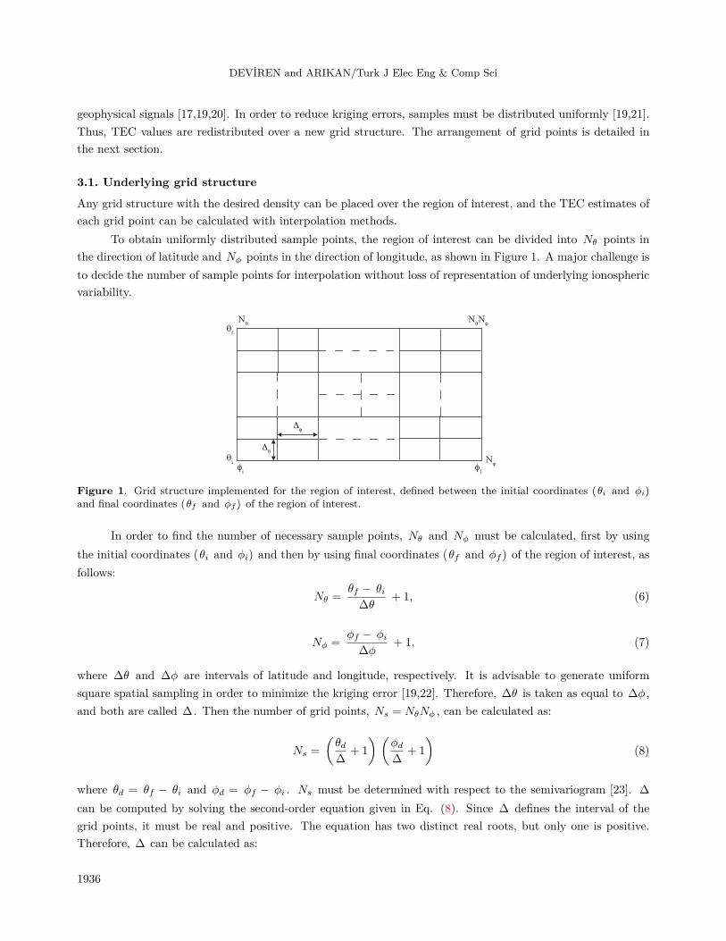
To obtain uniformly distributed sample points, the region of interest can be divided into Nθ points inthe direction of latitude and Nϕ points in the direction of longitude, as shown in Figure 1. A major challenge isto decide the number of sample points for interpolation without loss of representation of underlying ionosphericvariability.

θ

f

θi

φf

φi

Nθ

NθN

φ

Nφ

Δθ

Δφ

Figure 1. Grid structure implemented for the region of interest, defined between the initial coordinates (θi and ϕi)and final coordinates (θf and ϕf ) of the region of interest.

In order to find the number of necessary sample points, Nθ and Nϕ must be calculated, first by usingthe initial coordinates (θi and ϕi) and then by using final coordinates (θf and ϕf ) of the region of interest, asfollows:

Nθ =θf − θi∆θ

+ 1, (6)

Nϕ =ϕf − ϕi

∆ϕ+ 1, (7)

where ∆θ and ∆ϕ are intervals of latitude and longitude, respectively. It is advisable to generate uniformsquare spatial sampling in order to minimize the kriging error [19,22]. Therefore, ∆θ is taken as equal to ∆ϕ ,and both are called ∆ . Then the number of grid points, Ns = NθNϕ , can be calculated as:

Ns =

(θd∆

+ 1

) (ϕd

∆+ 1

)(8)

where θd = θf − θi and ϕd = ϕf − ϕi . Ns must be determined with respect to the semivariogram [23]. ∆

can be computed by solving the second-order equation given in Eq. (8). Since ∆ defines the interval of thegrid points, it must be real and positive. The equation has two distinct real roots, but only one is positive.Therefore, ∆ can be calculated as:

1936


∆ =(θd + ϕd) +

√(θd + ϕd)

2+ 4 θd ϕd (Ns − 1)

2 (Ns − 1). (9)

TEC estimates can be obtained using the interpolation algorithm on a redistributed uniform grid. Universalkriging with linear trend (UK1) and ordinary kriging algorithms are provided in the next section.

3.2. Automatic regional mapping using UK1 algorithmThe UK1 algorithm estimates TEC, zK , using the linear combination TEC samples, zs , at any position in

space, x =[θ ϕ

]T , where θ and ϕ denote latitude and longitude, respectively. zK can be calculated as:

zK (x) =

Nu∑nu=1

λnuzs (xnu

) (10)

where xnu=[θnu

ϕnu

]T defines the measurement points. Weight λnuat nu sample point is obtained by

solving the constrained optimization [14–17,19,20].The strength of the statistical correlation as a function of distance in kriging can be calculated by using

a semivariogram function. Since the experimental semivariogram may be computed only for certain pairs atirregular distances, h , a theoretical model is usually fitted to obtain a continuous function for all possible h

values. In the literature, typical theoretical semivariogram functions are chosen as exponential, Gaussian, andspherical [14,15].

In the case of the ionosphere, TEC values vary significantly with respect to time and one semivariogramfunction may not represent this complicated variability. Therefore, in this study, the theoretical semivariogramfunction is chosen to be the Matern family, which includes all the above-listed functions and is given as:

γM (h) =

{0 , h = 0

c0 + σ20

[2hν

(2d)ν Γ(ν) Kν(h/d)]

, h > 0

}(11)

where c0 is the nugget effect; σ20 is the partial sill; Kν(•) is the modified Bessel function of the second kind

and order ν ; and, finally, d is defined as the range [14–16]. Different correlation models can be obtained bychanging the smoothing parameter, ν .

Parameters c0 , σ20 , ν , and d can be obtained by using the particle swarm optimization (PSO) method

due to its heuristic nature. The advantages of PSO are its relative ease in implementation and convergencespeed for manipulating optimum points with few parameters [14–16,23].

The UK1 algorithm can be repeated for any desired temporal interval. Since the parameters of theMatern semivariogram function are obtained using PSO, the UK1 maps are obtained automatically with highspatial resolution for any desired time interval.

3.3. Automatic regional mapping using ordinary kriging algorithm

The ordinary kriging (OK) algorithm estimates TEC using the linear combination TEC samples at any positionin space x , as shown in Eq. (10). The main difference between UK1 and OK comes from the underlying trendestimation. OK assumes that TEC over a region has a fixed yet unknown trend. Unlike the UK1 algorithm,

1937


the experimental semivariogram is calculated directly over the TEC values for the OK algorithm. The Maternsemivariogram is chosen as the theoretical semivariogram function. By running the PSO algorithm several times,the parameters of the Matern function can be obtained with minimum cost with respect to the experimentalsemivariogram. Then the weights of the sample points given in Eq. (10) are obtained with respect to the OKalgorithm by solving the constrained optimization.

The OK algorithm can be repeated for any desired temporal interval. Since the parameters of theMatern semivariogram function are obtained using PSO, OK maps are obtained automatically with high spatialresolution for any desired time interval. In the next section, the results of the developed algorithms are explainedfor automatic mapping of TEC.

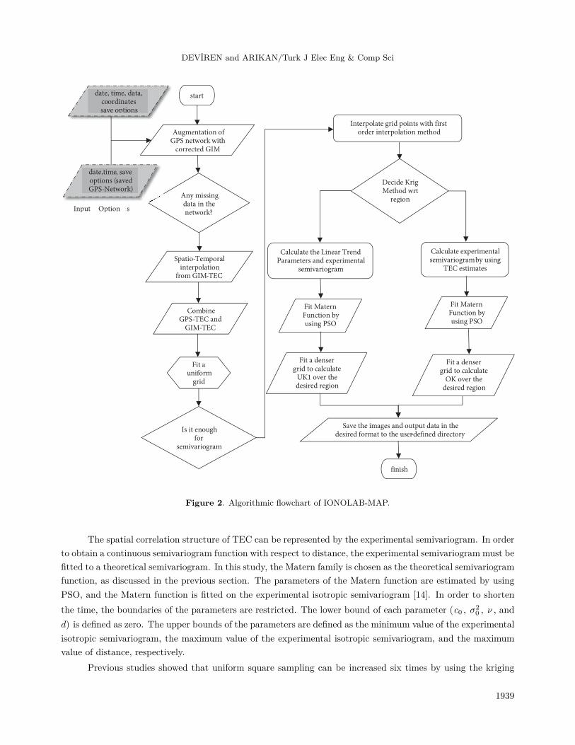
4. ResultsIn this study, a user-friendly, robust, reliable, and automatic regional spatial interpolation algorithm, calledIONOLAB-MAP, is developed. The outlined algorithm of IONOLAB-MAP, given in Figure 2, can be appliedto any GPS network. This algorithm operates with two different input options. GPS-TEC can be obtainedfrom a directory or given as an input. Before the augmentation of the GPS network with GIM-TEC, the valuesare checked and possible erroneous values are corrected using the methods given in [2,12,24]. For the purposeof reducing instabilities in kriging that occur in the inverse operation [19,20], GPS-TEC is augmented withcorrected GIM-TEC. After augmentation of GPS-TEC with GIM-TEC, the missing GPS-TECs are recoveredwith the spatiotemporal interpolation method given in Section 2. In order to reduce kriging errors, a uniformgrid structure is constituted over the given region. TEC estimates of the uniformly distributed grid points arecalculated using a first-order interpolation algorithm. With respect to the region, the algorithm chooses thekriging method automatically and high-resolution TEC maps are generated. Finally, the outputs are saved ina predetermined format in a user-defined directory.

In this study, IONOLAB-MAP is applied to the Turkish National Permanent GPS Network (TNPGN-Active). The TNPGN-Active network is composed of 144 GNSS stations, which have continuously operatedsince May 2009. TEC is estimated as IONOLAB-TEC, whose temporal resolution is 2.5 min [2,12,24]. However,the typical temporal resolution of GIM is 2 h. In order to equalize the temporal resolution of GIM-TECwith IONOLAB-TEC, GIM-TECs are interpolated by C-spline [15,16]. Then IONOLAB-TEC is augmentedwith corrected GIM-TEC, and the missing IONOLAB-TEC values are recovered based on the spatiotemporalinterpolation method provided in [15,16]. The disrupted IONOLAB-TEC values are interpolated with oneneighborhood (Nu;Rr

= 1) and one day (di = ds = d − 1) at a given time. Any TNPGN-Active station issurrounded by four GIM points. The disrupted IONOLAB-TEC of any TNPGN station is estimated from fourseparate GIM points. The new value of the missing IONOLAB-TEC is calculated by taking the median of thesefour different GIM-TEC values, temporally interpolated for the desired hour.

Before the kriging algorithm is implemented, the uniformly distributed grid structure given in Section 3.1is placed over Turkey. A common yet unsubstantiated practice is to limit estimation to lags with a minimumof 30 pairs in order to calculate the experimental semivariogram [17]. The number of grid points (Ns) isdetermined to provide minimum pairs. Then the TEC estimates of each grid point are calculated using theIDW algorithm. Hence, the TEC of each grid point is calculated from the weighted average of the sparser data.

As indicated previously, the underlying trend function must be known to process the UK1 algorithm.Previous studies show that the trend of TEC for a midlatitude region can be modeled by a linear function [25].Hence, in this study, the trend of the TNPGN-Active is chosen as linear [14–16].

1938


Augmentat on of GPS network w th

corrected GIM

Spat o-Temporal nterpolat on

from GIM-TEC

Any m ss ng data n the network?

start

Comb ne GPS-TEC and

GIM-TEC

F t a un form

gr d

Is t enough for

sem var ogram

Interpolate gr d po nts w th f rst order nterpolat on method

date,t me, save opt ons (saved GPS-Network)

date, t me, data, coord nates save opt ons

Dec de Kr g Method wrt

reg on

Calculate the L near Trend Parameters and exper mental

sem var ogram

Calculate exper mentalsem var ogramby us ng

TEC est mates

F t Matern Funct on by us ng PSO

F t Matern Funct on by us ng PSO

F t a denser gr d to calculate

UK1 over the des red reg on

F t a denser gr d to calculate

OK over the des red reg on

Save the mages and output data n the des red format to the user-def ned d rectory

f n sh

Input Opt on s

Figure 2. Algorithmic flowchart of IONOLAB-MAP.

The spatial correlation structure of TEC can be represented by the experimental semivariogram. In orderto obtain a continuous semivariogram function with respect to distance, the experimental semivariogram must befitted to a theoretical semivariogram. In this study, the Matern family is chosen as the theoretical semivariogramfunction, as discussed in the previous section. The parameters of the Matern function are estimated by usingPSO, and the Matern function is fitted on the experimental isotropic semivariogram [14]. In order to shortenthe time, the boundaries of the parameters are restricted. The lower bound of each parameter (c0 , σ2

0 , ν , andd) is defined as zero. The upper bounds of the parameters are defined as the minimum value of the experimentalisotropic semivariogram, the maximum value of the experimental isotropic semivariogram, and the maximumvalue of distance, respectively.

Previous studies showed that uniform square sampling can be increased six times by using the kriging

1939


algorithm [19,20]. Thus, in this study, in order to obtain denser TEC maps, TEC estimates are redistributedon a high spatial resolution (six times larger) grid structure. The number of grid points, N

′

s , can be found asN

′

s = 6Ns after the kriging algorithm. TEC estimation of each new grid point is calculated using UK1, givenin Section 3.2, and the IONOLAB-MAP is generated. Lastly, IONOLAB-MAP and data can be saved in apredetermined format.

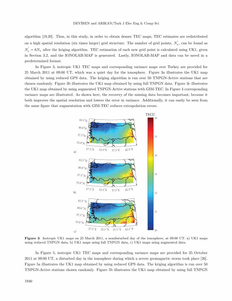
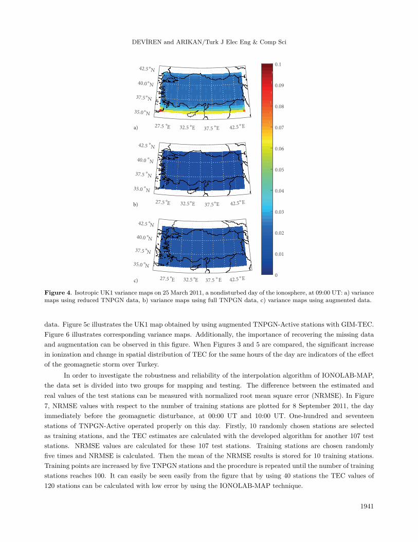
In Figure 3, isotropic UK1 TEC maps and corresponding variance maps over Turkey are provided for25 March 2011 at 09:00 UT, which was a quiet day for the ionosphere. Figure 3a illustrates the UK1 mapobtained by using reduced GPS data. The kriging algorithm is run over 50 TNPGN-Active stations that arechosen randomly. Figure 3b illustrates the UK1 map obtained by using full TNPGN data. Figure 3c illustratesthe UK1 map obtained by using augmented TNPGN-Active stations with GIM-TEC. In Figure 4 correspondingvariance maps are illustrated. As shown here, the recovery of the missing data becomes important, because itboth improves the spatial resolution and lowers the error in variance. Additionally, it can easily be seen fromthe same figure that augmentation with GIM-TEC reduces extrapolation errors.

27.5 ° E 32.5° E 37.5° E 42.5° E

35.0 ° N

37.5 ° N

40.0 ° N

42.5 ° N

20

21

22

23

24

25

26

TECU

27.5 ° E 32.5° E 37.5° E 42.5° E

35.0 ° N

37.5 ° N

40.0 ° N

42.5 ° N

42.5 ° E 37.5 ° E 32.5 ° E 27.5 ° E

35.0 ° N

37.5 ° N

40.0 ° N

42.5 ° N

a)

b)

c)

Figure 3. Isotropic UK1 maps on 25 March 2011, a nondisturbed day of the ionosphere, at 09:00 UT: a) UK1 mapsusing reduced TNPGN data, b) UK1 maps using full TNPGN data, c) UK1 maps using augmented data.

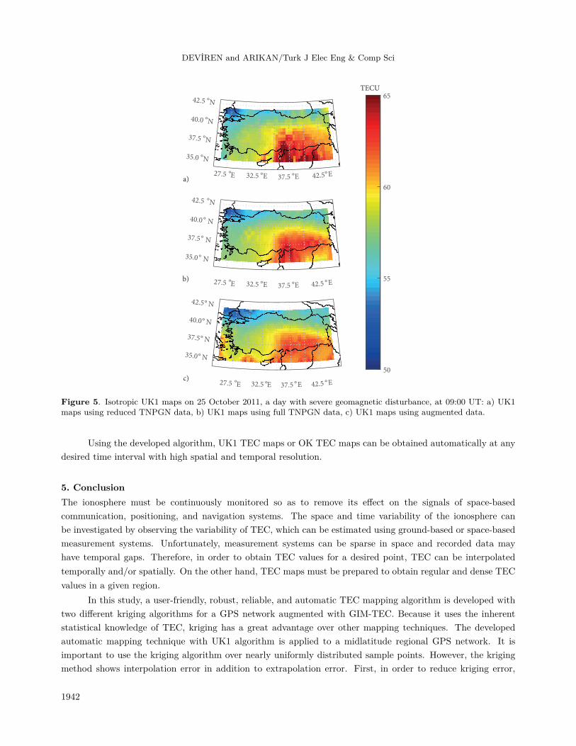
In Figure 5, isotropic UK1 TEC maps and corresponding variance maps are provided for 25 October2011 at 09:00 UT, a disturbed day in the ionosphere during which a severe geomagnetic storm took place [26].Figure 5a illustrates the UK1 map obtained by using reduced GPS data. The kriging algorithm is run over 50TNPGN-Active stations chosen randomly. Figure 5b illustrates the UK1 map obtained by using full TNPGN

1940


27.5 ° E 32.5 ° E 37.5 ° E 42.5 ° E

35.0° N

37.5° N

40.0° N

42.5° N

0

0.01

0.02

0.03

0.04

0.05

0.06

0.07

0.08

0.09

0.1

27.5 ° E 32.5° E 37.5° E 42.5° E

35.0 ° N

37.5 ° N

40.0 ° N

42.5 ° N

27.5 ° E 32.5 ° E 37.5 ° E 42.5 ° E

35.0 ° N

37.5 ° N

40.0 ° N

42.5 ° N

a)

b)

c)

Figure 4. Isotropic UK1 variance maps on 25 March 2011, a nondisturbed day of the ionosphere, at 09:00 UT: a) variancemaps using reduced TNPGN data, b) variance maps using full TNPGN data, c) variance maps using augmented data.

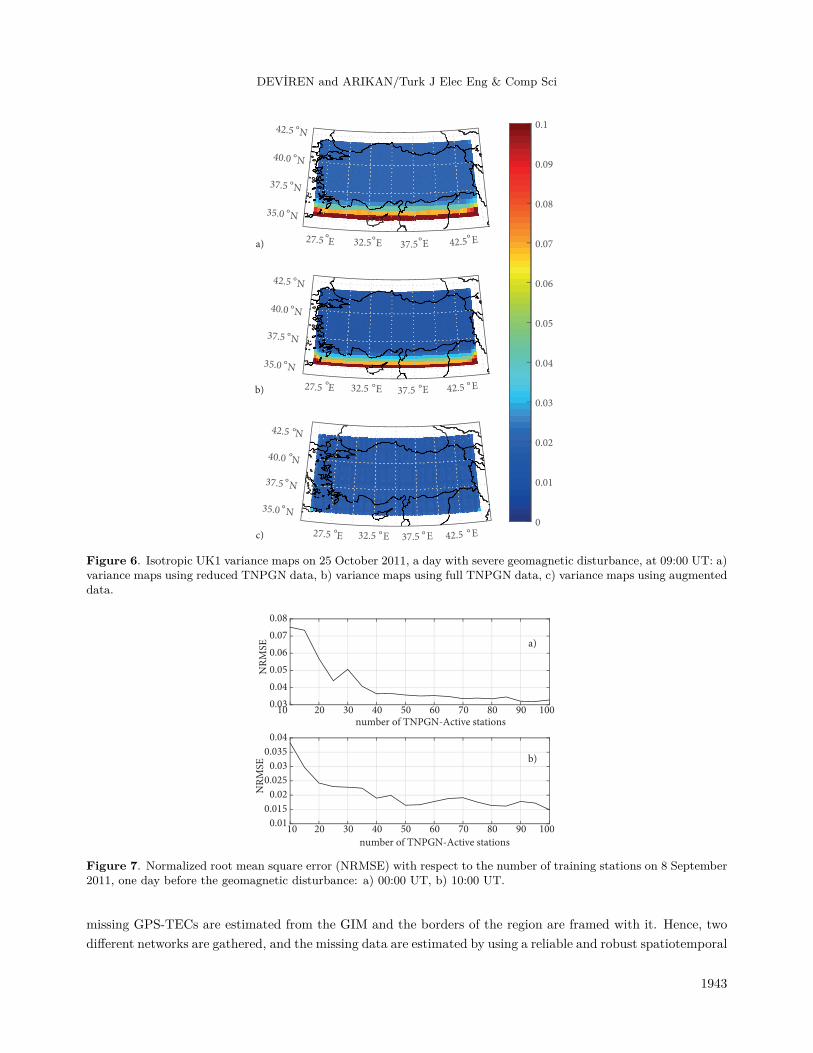
data. Figure 5c illustrates the UK1 map obtained by using augmented TNPGN-Active stations with GIM-TEC.Figure 6 illustrates corresponding variance maps. Additionally, the importance of recovering the missing dataand augmentation can be observed in this figure. When Figures 3 and 5 are compared, the significant increasein ionization and change in spatial distribution of TEC for the same hours of the day are indicators of the effectof the geomagnetic storm over Turkey.

In order to investigate the robustness and reliability of the interpolation algorithm of IONOLAB-MAP,the data set is divided into two groups for mapping and testing. The difference between the estimated andreal values of the test stations can be measured with normalized root mean square error (NRMSE). In Figure7, NRMSE values with respect to the number of training stations are plotted for 8 September 2011, the dayimmediately before the geomagnetic disturbance, at 00:00 UT and 10:00 UT. One-hundred and seventeenstations of TNPGN-Active operated properly on this day. Firstly, 10 randomly chosen stations are selectedas training stations, and the TEC estimates are calculated with the developed algorithm for another 107 teststations. NRMSE values are calculated for these 107 test stations. Training stations are chosen randomlyfive times and NRMSE is calculated. Then the mean of the NRMSE results is stored for 10 training stations.Training points are increased by five TNPGN stations and the procedure is repeated until the number of trainingstations reaches 100. It can easily be seen easily from the figure that by using 40 stations the TEC values of120 stations can be calculated with low error by using the IONOLAB-MAP technique.

1941


27.5 ° E 32.5 ° E 37.5 ° E 42.5° E

35.0 ° N

37.5 ° N

40.0 ° N

42.5 ° N

50

55

60

65TECU

27.5 ° E 32.5 ° E 37.5 ° E 42.5 ° E

35.0° N

37.5° N

40.0° N

42.5 ° N

27.5 ° E 32.5 ° E 37.5 ° E 42.5 ° E

35.0° N

37.5° N

40.0° N

42.5° N

a)

b)

c)

Figure 5. Isotropic UK1 maps on 25 October 2011, a day with severe geomagnetic disturbance, at 09:00 UT: a) UK1maps using reduced TNPGN data, b) UK1 maps using full TNPGN data, c) UK1 maps using augmented data.

Using the developed algorithm, UK1 TEC maps or OK TEC maps can be obtained automatically at anydesired time interval with high spatial and temporal resolution.

5. ConclusionThe ionosphere must be continuously monitored so as to remove its effect on the signals of space-basedcommunication, positioning, and navigation systems. The space and time variability of the ionosphere canbe investigated by observing the variability of TEC, which can be estimated using ground-based or space-basedmeasurement systems. Unfortunately, measurement systems can be sparse in space and recorded data mayhave temporal gaps. Therefore, in order to obtain TEC values for a desired point, TEC can be interpolatedtemporally and/or spatially. On the other hand, TEC maps must be prepared to obtain regular and dense TECvalues in a given region.

In this study, a user-friendly, robust, reliable, and automatic TEC mapping algorithm is developed withtwo different kriging algorithms for a GPS network augmented with GIM-TEC. Because it uses the inherentstatistical knowledge of TEC, kriging has a great advantage over other mapping techniques. The developedautomatic mapping technique with UK1 algorithm is applied to a midlatitude regional GPS network. It isimportant to use the kriging algorithm over nearly uniformly distributed sample points. However, the krigingmethod shows interpolation error in addition to extrapolation error. First, in order to reduce kriging error,

1942


27.5 ° E 32.5° E 37.5° E 42.5° E

35.0 ° N

37.5 ° N

40.0 ° N

42.5 ° N

0

0.01

0.02

0.03

0.04

0.05

0.06

0.07

0.08

0.09

0.1

27.5 ° E 32.5 ° E 37.5 ° E 42.5 ° E

35.0 ° N

37.5 ° N

40.0 ° N

42.5 ° N

27.5 ° E 32.5 ° E 37.5 ° E 42.5 ° E

35.0 ° N

37.5 ° N

40.0 ° N

42.5 ° N

a)

b)

c)

Figure 6. Isotropic UK1 variance maps on 25 October 2011, a day with severe geomagnetic disturbance, at 09:00 UT: a)variance maps using reduced TNPGN data, b) variance maps using full TNPGN data, c) variance maps using augmenteddata.

number of TNPGN-Active stations

10 20 30 40 50 60 70 80 90 100

NR

MS

E

0.03

0.04

0.05

0.06

0.07

0.08

number of TNPGN-Active stations

10 20 30 40 50 60 70 80 90 100

NR

MS

E

0.01

0.015

0.02

0.025

0.03

0.035

0.04

b)

a)

Figure 7. Normalized root mean square error (NRMSE) with respect to the number of training stations on 8 September2011, one day before the geomagnetic disturbance: a) 00:00 UT, b) 10:00 UT.

missing GPS-TECs are estimated from the GIM and the borders of the region are framed with it. Hence, twodifferent networks are gathered, and the missing data are estimated by using a reliable and robust spatiotemporal

1943


interpolation technique. Therefore, the novel mapping algorithm, which differs from other mapping techniquesby using the estimation algorithm, operates with minimum error in all circumstances. In order to calculate theexperimental semivariogram, the first-order interpolation method is used for grid points, which are arrangedautomatically. Then the Matern function is fitted on the experimental isotropic semivariogram using a nonlinearoptimization routine, PSO. Additionally, grid size is arranged to optimize the number of sample points, and thealgorithm automatically switches between universal and ordinary kriging according to the region. Hence, highspace-time resolution automatic kriging maps are obtained and the outputs can be saved in the desired formatin the user-defined directory.

Acknowledgment

This study was supported by the grants of TÜBİTAK 115E915 and TÜBİTAK 114E541 and the joint TÜBİTAK112E568 and RFBR 13-02-91370-CT a projects.

References

[1] Moon Y. Evaluation of 2-dimensional ionosphere models for national and regional GPS networks in Canada. MSc,University of Calgary, Calgary, Canada, 2004.

[2] Arıkan F, Erol CB, Arıkan O. Regularized estimation of vertical total electron content from GPS data for a desiredtime period. Radio Sci 2004; 39: 1-10.

[3] Komjathy A. Global ionospheric total electron content mapping using the Global Positioning System. PhD, Uni-versity of New Brunswick, Fredericton, Canada, 1997.

[4] Hernández-Pajares M, Juan JM, Sanz J, Orus R, Garcia-Rigo A, Feltens J, Komjath A, Schaer SC, Krankowski A.The IGS VTEC map: a reliable source of ionospheric information since 1998. J Geodesy 2009; 83: 263-275.

[5] Yılmaz A, Akdoğan KE, Gürün M. Regional TEC mapping using neural networks. Radio Sci 2009; 44: RS3007.

[6] Habarulema JB, McKinnell LA, Cilliers PJ. Prediction of global positioning system total electron content usingneural networks over South Africa. J Atmos Sol-Terr Phy 2007; 69: 1842-1850.

[7] Hardly RL. Multiquadratic equations of topography and other irregular surfaces. J Geophys Res 1971; 76: 1905-1915.

[8] Jin S, Wang J, Zhang H, Zhu W. Real-time monitoring and prediction of ionospheric electron content by means ofGPS. Chinese Astron Astr 2004; 28: 331-337.

[9] Wielgosz P, Brzezinska D, Kashani I. Regional ionosphere mapping with kriging and multiquadratic method. JGlob Pos Sys 2003; 2: 48-55.

[10] Ghoddousi-Fard R, Héroux P, Danskin D, Boteler D. Developing a GPS TEC mapping service over Canada. AdvSpace Res 2011; 9: S06D11.

[11] Bouya Z, Terkildsen M, Neudegg D. Regional GPS-based ionospheric TEC model over Australia using sphericalcap harmonic analysis. In: ICSU 2010 COSPAR Scientific Assembly; 15–18 July 2010; Bremen, Germany. Paris,France: International Council for Science. p. 4.

[12] Arıkan F, Yılmaz A, Arıkan O, Sayın I, Gürün M, Akdoğan KE, Yıldırım SA. Space weather activities of IONOLABGroup: TEC mapping. In: EGU 2009 General Assembly; 19–24 April 2009; Vienna, Austria. Munich, Germany:EGU. p. 6962.

[13] Aa E, Huang W, Yu S, Liu S, Shi L, Gong J, Chen Y, Shen H. A regional ionospheric TEC mapping technique overChina and adjacent areas on the basis of data assimilation. J Geophys Res 2015; 120: 5049-5061.

1944


[14] Deviren MN, Arıkan F, Arıkan O. Automatic regional mapping of total electron content using a GPS sensor networkand isotropic universal kriging. In: IEEE 2013 International Conference on Information Fusion; 9–12 July 2013;İstanbul, Turkey. New York, NY, USA: IEEE. pp. 1664-1669.

[15] Deviren MN. Estimation of space-time random field for total electron content (TEC) over Turkey. MSc, HacettepeUniversity, Ankara, Turkey, 2013.

[16] Deviren MN, Arıkan F, Arıkan O. Spatio-temporal interpolation of total electron content using a GPS network.Radio Sci 2013; 48: 302-309.

[17] Olea RA. Geostatistics for Engineers and Earth Scientists. New York, NY, USA: Springer, 1999.

[18] Orús R, Hernández-Pajares M, Juan JM, Sanz J. Improvement of global ionospheric VTEC maps by using kriginginterpolation technique. J Atmos Sol-Terr Phy 2005; 67: 1598-1609.

[19] Sayın I. Total electron content mapping using kriging and random field priors. MSc, Hacettepe University, Ankara,Turkey, 2008.

[20] Sayın I, Arıkan F, Arıkan O. Regional TEC mapping with random field priors and kriging. Radio Sci 2008; 43:RS5012.

[21] Yfantis EA, Flatman GT, Behar JV. Efficiency of kriging estimation for square, triangular, and hexagonal grids.Math Geol 1987; 19: 183-205.

[22] Schaer S. Mapping and predicting the Earth’s ionosphere using the Global Positioning System. PhD, University ofBern, Bern, Switzerland, 1999.

[23] Haupt RL, Haupt SE. Practical Genetic Algorithms. 2nd ed. New York, NY, USA: Wiley, 2004.

[24] Arıkan F, Sezen U, Gulyaeva TL, Çilibaş O. Online, automatic, ionospheric maps:IRI-PLAS-MAP. Adv Space Res2015; 55: 2106-2113.

[25] Toker C, Gökdağ YE, Arıkan F, Arıkan O. Application of modified particle swarm Optimization method forparameter extraction of 2-D TEC mapping. In: EGU 2012 General Assembly; 22–27 April 2012; Vienna, Austria.Munich, Germany: EGU. p. 7501.

[26] Blanch, E, Marsal S, Segarra A, Torta JM, Altadill D, Curto JJ. Space weather effects on Earth’s environmentassociated to the 24–25 October 2011 geomagnetic storm. Adv Space Res 2013; 11: 153-168.

1945

ionolab-map: an automatic spatial interpolation algorithm...

Documents