ionospheric disturbance on gnss receivers and other systems
TRANSCRIPT

Improving landfill monitoring programswith the aid of geoelectrical - imaging techniquesand geographical information systems Master’s Thesis in the Master Degree Programme, Civil Engineering
KEVIN HINE
Department of Civil and Environmental Engineering Division of GeoEngineering Engineering Geology Research GroupCHALMERS UNIVERSITY OF TECHNOLOGYGöteborg, Sweden 2005Master’s Thesis 2005:22
Obs.1 Obs.2Mid.Obs.
SilentIonosphere
FluctuatingIonosphere
GPS Signals
δ1
Δ2
δ2Δm
Δ1
Ionospheric Disturbance on GNSSReceivers and Other Systems
Master’s thesis in Radio and Space Science
WEIHUA WANG
Department of Earth and Space SciencesChalmers University of TechnologyGothenburg, Sweden 2015


THESIS FOR THE DEGREE IN MASTER OF SCIENCE
Ionospheric Disturbance on GNSS Receiversand Other Systems
Weihua Wang
Department of Earth and Space SciencesChalmers University of Technology
Gothenburg, Sweden 2015

Ionospheric Disturbance on GNSS Receivers and Other SystemsWeihua Wang
c© Weihua Wang, 2015.
Supervisor: Per Jarlemark, SP Technical Research Institute of SwedenExaminer: Jan Johansson, Department of Earth and Space Sciences
Master of Science ThesisDepartment of Earth and Space SciencesResearch Group of Space Geodesy and GeodynamicsChalmers University of TechnologySE-412 96 GothenburgTelephone +46 31 772 1000
iii

Dedicated to my parents Hanxing Wang and Fang Wang
iv

Ionospheric Disturbances on GPS Receivers and Other SystemsWeihua WangDepartment of Earth and Space SciencesChalmers University of Technology
Abstract
Equatorial ionospheric plasma irregularities are generated at the magneticequator areas after sunset due to plasma instabilities. Its impact on the GPS(Global Positioning System) signals, both amplitude and phase, often resultsin a degraded performance of the GPS receivers. Based on observational dataobtained from dual-frequency GPS receivers at two triangular observationalnetworks in south Brazil, ionospheric variability over one full year range(2013) is studied through the Total Electron Content (TEC) distribution.Small-scaled local TEC variations of the region of two observational networksare also presented. From characterization of the local TEC variations, it isthought to be primarily related to the local Equatorial Plasma Bubbles’(EPBs) activities due to the Equatorial Ionospheric Anomaly (EIA).
Keywords: GPS signals, TEC, equatorial plasma irregularities.
v

Acknowledgements
The author would like to sincerely thank Professor Jan Johansson of ChalmersUniversity of Technology, and Dr. Per Jarlemark at SP Technical ResearchInstitute of Sweden for their significant and kind help in theoretical guidance,simulations, supervision and comments on this project.
Weihua Wang, Gothenburg, May 2015

List of Abbreviations
BRDC Broadcast Ephemeris Data
C/A-code Coarse/acquisition code
CDMA Code Division Multiple Access
DOP Dilution Of Precision
EIA Equatorial Ionospheric Anomaly
EPBs Equatorial Plasma Bubbles
ESA European Space Agency
IOC Initial Operational Capability
FOC Full Operational Capability
GLONASS Globalnaya Navigazionnaya Sputnikovaya Sistema
GNSS Global Navigation Satellite System
GPS Global Positioning System
GRT Generalized Rayleigh-Taylor
IAACs Ionosphere Associate Analysis Centers
IBGE Instituto Brasileiro de Geografia e Estatstica
IGS International GNSS Service
IOC Initial Operational Capability
IONEX format IONospheric map EXchange ASCII format
IPP Ionospheric Pierce Point
JPL Jet Propulsion Laboratory
LOS Line Of Sight
LSTIDs Large Scale Traveling Ionospheric Disturbances
MCS Master Control Station
vii

MSTIDs Medium Scale Traveling Ionospheric Disturbances
NBI Narrow-band Interference
NASA National Aeronautics and Space Administration
P-code Precision code
PRN Pseudo-random Noise
SAA South Atlantic Anomaly
SID Sudden Ionospheric Disturbance
SPENVIS Space Environment Information System
STEC Slant Total Electron Content
SV Space Vehicles
TEC Total Electron Content
TECU Total Electron Content Unit
TID Traveling Ionospheric Disturbance
TOA Time Of Arrival
UERE User Equivalent Range Error
UT Universal Time
VTEC Vertical Total Electron Content
viii

Contents
List of Figures x
List of Tables xii
1 Introduction 1
2 GPS Background 22.1 GPS Overview . . . . . . . . . . . . . . . . . . . . . . . . . . . 22.2 GPS Segments . . . . . . . . . . . . . . . . . . . . . . . . . . . 32.3 GPS Signals . . . . . . . . . . . . . . . . . . . . . . . . . . . . 62.4 Code Pseudo-range Measurements . . . . . . . . . . . . . . . . 82.5 Carrier Phase Measurements . . . . . . . . . . . . . . . . . . . 112.6 Doppler Measurements . . . . . . . . . . . . . . . . . . . . . . 122.7 Errors and Biases . . . . . . . . . . . . . . . . . . . . . . . . . 13
3 Ionosphere Background 163.1 Height Characteristics . . . . . . . . . . . . . . . . . . . . . . 173.2 Ionosphere Variation Types . . . . . . . . . . . . . . . . . . . 18
3.2.1 General Variations of Global Scale . . . . . . . . . . . 183.2.2 Specific Variations Around Tropical Areas . . . . . . . 19
4 Signal Propagation through the Ionosphere 234.1 Some Fundamentals of Wave Propagation . . . . . . . . . . . 234.2 Ionospheric Refraction . . . . . . . . . . . . . . . . . . . . . . 25
5 Methodology of Obtaining the Ionospheric Variability 30
6 Data Set 33
7 Results and Discussion 367.1 swTEC Analysis . . . . . . . . . . . . . . . . . . . . . . . . . 367.2 Correlation Study . . . . . . . . . . . . . . . . . . . . . . . . . 39
ix

7.3 Comparison of TEC and swTEC . . . . . . . . . . . . . . . . 407.4 Conclusion . . . . . . . . . . . . . . . . . . . . . . . . . . . . . 437.5 Future Work . . . . . . . . . . . . . . . . . . . . . . . . . . . . 44
References 45
Appendix A Methodology for Estimating the Ionospheric Vari-ability I
Appendix B Observational Data Set IV
x

List of Figures
2.1 Illustration of satellite positioning via an intersection of threespheres, where the clock icons represent orbital satellites. . . . 3
2.2 GPS constellation of 24 satellites. . . . . . . . . . . . . . . . . 32.3 Initial deployment of GPS control sites. . . . . . . . . . . . . . 52.4 Major components of a GPS receiver, redrawn from [1]. . . . . 52.5 GPS segments illustration, redrawn from [2]. . . . . . . . . . . 62.6 An illustration of the pseudo-range measurements (Note: ∆t
= signal propagation time), redrawn from [3]. . . . . . . . . . 92.7 Major components of GPS errors and biases, redrawn from [3]. 132.8 Good and bad satellite geometry illustration. . . . . . . . . . . 15
3.1 Illustration of the ionospheric layers in daytime and nighttime. 173.2 World geomagnetic inclination in South American regions [4]. 213.3 Main magnetic field at Earth’s surface in June 2014 [5]. . . . . 223.4 SPENVIS simulation of SAA at 550 km. Note that values in
the index bar are logarithmic. . . . . . . . . . . . . . . . . . . 22
4.1 Ionospheric single layer model illustration, redrawn from [1]. . 27
5.1 An illustration of linear interpolation. . . . . . . . . . . . . . . 31
6.1 Map of the eight selected Brazilian observational sites. . . . . 34
7.1 Local ionospheric variability comparison for the two observa-tional networks of a whole 2013 year. . . . . . . . . . . . . . . 37
7.2 Histogram plot showing the occurrence frequency of the swTECunit. Median value: 1.4392 (top) and 0.9677 (below). . . . . . 38
7.3 Whole year range correlation plot. . . . . . . . . . . . . . . . . 397.4 Correlation plot from April to August. . . . . . . . . . . . . . 397.5 Illustration of plasma bubble observation. . . . . . . . . . . . . 407.6 Whole year TEC and swTEC comparison. . . . . . . . . . . . 417.7 Spacial high-pass filtering effect can be resolved by the local
observational network. . . . . . . . . . . . . . . . . . . . . . . 43
xi

List of Tables
2.1 Basic characteristic features of the GPS [1] . . . . . . . . . . . 42.2 The GPS satellite signals [1] . . . . . . . . . . . . . . . . . . . 82.3 The navigation message format [6] . . . . . . . . . . . . . . . . 82.4 Sources of User Equivalent Range Errors [6] . . . . . . . . . . 15
3.1 MSTIDs and LSTIDs . . . . . . . . . . . . . . . . . . . . . . . 20
B.1 Specific date used from IBGE website each Thursday . . . . . IV
xii

Chapter 1
Introduction
Intense ionospheric disturbance can lead to unwanted terrestrial consequencessuch as malfunctioning satellite communications and navigation, as well aselectric power grids. As the GNSS (Global Navigation Satellite System) ra-dio signal propagating through the atmosphere, ionospheric variation will notonly affect the signal velocity, resulting in phase advance and group delay,but also bend the signal. Strong amplitude fading and phase distortion dueto violent ionospheric disturbances will degrade the navigation performancea lot. Therefore, understanding the causes and mitigating the impact of theionospheric disturbance is quite important.
Equatorial regions in Brazil can sometimes experience severe problems as-sociated with ionospheric irregularities, mainly due to influences of the solaractivities, daily and seasonal variations due to movement of the Earth, andabnormal distribution of the geomagnetic field. However, still need to fur-ther investigate, the ionospheric variations over Brazilian territory seems itmay influence applications such as the calculation of the atomic time scalefor satellite-based timing services and positioning at aviation traffic control.
The main purpose of this project is to study the ionospheric variability overBrazil. Characterization of the electron distribution variations, representedby the Total Electron Content (TEC), are analyzed from both temporal andspatial point of view, based on local observational data continuously recordedfrom geographically distributed GNSS receivers in southern Brazil. In ad-dition, equatorial ionospheric anomaly, supposed to be closely related withactivities of the Equatorial Plasma Bubbles (EPBs), has been preliminary ex-plored and compared with outcome from the Vertical Total Electron Content(VTEC) map produced by the Ionosphere Working Group of InternationalGNSS Service (IGS).
1

Chapter 2
GPS Background
2.1 GPS Overview
The satellite-based Global Positioning System (GPS) can provide precisecontinuous positioning, timing information and speed to any user equippedwith a GPS receiver near the Earth surface. The GPS operates independentof weather conditions or geospatial restrictions as long as unobstructed line-of-sight (LOS) communication links to four or more GPS satellites are setup [3]. Basic features of the GPS are displayed in Table 2.1 [1].
The fundamental idea behind GPS is to measure the distances between aGPS receiver and several simultaneously LOS satellites. Since a user wantto utilize the GPS satellite constellation to perform positioning and naviga-tion, information about the satellite coordinates must be known in advance.Then the time of arrival (TOA) measurement, which aims to measure thesignal propagation time between the satellite and the receiver, is performed.By multiplying the signal propagation time with the speed of the light, thesatellite-to-receiver range can be computed. Finally, position of the receivercan be achieved by applying several TOA measurements with respect to mul-tiple visible satellites.
Theoretically, three distances between the GPS receiver and three simulta-neously visible satellites can be used to solve the user’s 3D position (latitude,longitude and altitude). In this case, location of the receiver is resulting froman intersection of three spheres. Each has a radius of one receiver-to-satelliterange and is centered on that particular satellite. A fourth satellite is addedto solve the receiver clock offset [7]. In practice, more than four satellitesare always visible for reliability and availability purposes. Figure 2.1 showsthat a specific position can be determined from an intersection of the threespheres.
2

Figure 2.1: Illustration of satellite positioning via an intersection of threespheres, where the clock icons represent orbital satellites.
2.2 GPS Segments
GPS consists of three segments, namely the space, control and user segment.The space segment includes on-orbit operational satellites, or space vehicles(SV) in GPS jargon, and its constellation. Initially 24 active SVs, geometryof the constellation is carefully designed such that four satellites are placedin each of six inclined orbital planes. As a result, more than four GPS satel-lites are simultaneously visible anywhere on the ground worldwide, as longas a LOS propagation is fulfilled. This constellation was known as the initialoperational capability (IOC) and is illustrated in Figure 2.2 by a MATLABsimulation. Since the GPS achieved its full operational capability (FOC)
Figure 2.2: GPS constellation of 24 satellites.
3
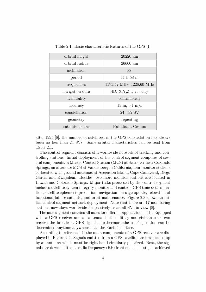
Table 2.1: Basic characteristic features of the GPS [1]
orbital height 20220 km
orbital radius 26600 km
inclination 55◦
period 11 h 58 m
frequencies 1575.42 MHz, 1228.60 MHz
navigation data 4D: X,Y,Z,t; velocity
availability continuously
accuracy 15 m, 0.1 m/s
constellation 24 - 32 SV
geometry repeating
satellite clocks Rubidium, Cesium
after 1995 [8], the number of satellites, in the GPS constellation has alwaysbeen no less than 24 SVs. Some orbital characteristics can be read fromTable 2.1.
The control segment consists of a worldwide network of tracking and con-trolling stations. Initial deployment of the control segment composes of sev-eral components: a Master Control Station (MCS) at Schriever near ColoradoSprings, an alternate MCS at Vandenberg in California, four monitor stationsco-located with ground antennas at Ascension Island, Cape Canaveral, DiegoGarcia and Kwajalein. Besides, two more monitor stations are located inHawaii and Colorado Springs. Major tasks processed by the control segmentincludes satellite system integrity monitor and control, GPS time determina-tion, satellite ephemeris prediction, navigation message update, relocation offunctional failure satellite, and orbit maintenance. Figure 2.3 shows an ini-tial control segment network deployment. Note that there are 17 monitoringstations nowadays worldwide for passively track all SVs in view [8].
The user segment contains all users for different application fields. Equippedwith a GPS receiver and an antenna, both military and civilian users canreceive the broadcast GPS signals, furthermore the user’s position can bedetermined anytime anywhere near the Earth’s surface.
According to reference [1] the main components of a GPS receiver are dis-played in Figure 2.4. Signals emitted from a GPS satellite are first picked upby an antenna which must be right-hand circularly polarized. Next, the sig-nals are down-shifted at radio frequency (RF) front end. This step is achieved
4

0 60 120 180 240 300 360−90
−60
−30
0
30
60
90
Longitude
Latit
ude
Master Control StationMonitor StationGround Antenna
Figure 2.3: Initial deployment of GPS control sites.
by a mixer which combines the incoming RF signals with a sinusoidal signalgenerated from a local oscillator, resulting in intermediate frequency (IF)signals. The down-converted IF signals are immediately forwarded to a sig-nal processor where algorithms of signal tracking and cross correlation areperformed. The received signals tracking from all visible satellites, at thisstep, are isolated, identified by their codes, and assigned for further process-ing. The microprocessor controls the receiver’s operation, including digitalsignal processing, decoding of the broadcast navigation message, control ofthe signal processor, on-line positions and velocities computation, and so on.The user communication part serves as a bridge between the user and themicroprocessor, with common tasks such as accepting commands from theuser, displaying of computing results and so on. Data logger and memorydevices store the data for further post-processing. Power supply provides lowvoltage DC power for the entire GPS receiver.
In conclusion, the space and control segments are developed and operatedby the U.S. Air Force. Each GPS receiver of the user segment utilizes the
AntennaPreamplifier Data logger
PowerSupply
SignalProcessor
Oscillator Usercommunication
MicroprocessorNavigation
solution
Figure 2.4: Major components of a GPS receiver, redrawn from [1].
5

Spread Spectrum
Ranging Signals & Navigation Data
Clock & Ephemeris
Space Segment
User Segment
Control Segment
Figure 2.5: GPS segments illustration, redrawn from [2].
broadcast satellite signals to acquire its 3D position and the current timeinformation. The three segments of GPS are collectively illustrated in Fig-ure 2.5.
2.3 GPS Signals
Generally, signal emitted from each satellite includes several components:two sine waves, three digital codes and a navigation message. The L-band(radio spectrum range between 1 and 2 GHz) sine waves, also known as carrierfrequencies, are coherently derived from the fundamental frequency of 10.23MHz (see Eq.(2.1)) which is generated by the space-borne highly accurateatomic oscillator. Accessibility of the L1 and L2 carrier allows for correctingthe ionospheric delay error which will be discussed in later chapters.
L1 : 154× 10.23 MHz = 1575.42 MHz
L2 : 120× 10.23 MHz = 1227.60 MHz (2.1)
The digital codes and navigation message are transmitted by each satel-lite on both carriers. In order to minimize the signal interference amongadjacent satellites and to save the scarce frequency resource, code divisionmultiple access (CDMA) is used so that all GPS satellites transmit with thesame frequency. Moreover, spread spectrum technique which resists against
6

narrow-band interference (NBI, typically emanates from radio stations ormobile phones), noise and jamming is used for security and power-savingpurposes. Both the carriers and the codes are used primarily to measure therange from the satellite transmitter to the GPS receiver.
The carriers are modulated with pseudo-random noise (PRN) codes, orpseudo-random binary sequences. The noise-like property of the PRN codesresult in a very low correlation with any other sequence generated by othersatellites or with the sequence itself but at different time. In addition, thecorrelation of the PRN code with the NBI, or with the thermal noise, is alsovery low which strengthen the noise resistance ability. Another advantage ofthe PRN code lie in its periodicity, hence certain mathematical expressionexists in order to generate the same PRN code. This makes satellite-to-receiver distance calculation feasible. In theory, if both the transmitter andthe receiver generate exactly the same PRN code, a very high correlationbetween the replica sequence generated by the local GPS receiver and thetransmitted sequence produced by the satellite could be achieved as long asboth clocks of the receiver and the transmitter are synchronized.
Traditional GPS satellites transmit two navigation codes known as coarseacquisition code (C/A-code) and precision code (P-code). Both digital codesare in fact the PRN codes. Historically, the P-code is modulated onto boththe L1 and L2 carriers, while the C/A-code is only available on the L1 car-riers. Although relatively less precise compared with that of the authorizedP-code, less complexity of the C/A-code enable all users to use it for rangemeasurement. The P-code is the principal navigation ranging code. How-ever, it is so long and complex so that a GPS receiver could not directlyacquire and synchronize with it alone. In real application, the receiver wouldfirst lock onto the simple C/A-code and then, after extracting informationof the current time and approximate position coordinates, synchronize withthe P-code later. A third code type, known as the P(Y)-code, is utilizedwherever the anti-spoofing mode of operation is required. The P(Y)-code isencrypted by multiplying the P-code with highly classified W-code [9]. Thisindicates that the primary users of the P(Y)-code belong to the U.S. militarysections. A summary of the GPS signal types are listed at Table 2.2 [1].
With a bitrate of 50 bits per second (bps), the navigation message trans-mitted by every satellite includes all the necessary information about theoperational satellites and the constellation, such as ‘health’ status, orbitalelements, clock behavior and other system parameters. Additionally, an al-manac is also provided which offers the approximate data for each activesatellite [8]. Each complete navigation message contains five sub-frames. Abrief description of each sub-frame can be read from Table 2.3 [6].
7

Table 2.2: The GPS satellite signals [1]
Atomic clock fundamental frequency 10.23 MHz
L1 carrier signal 154 × 10.23 MHz
L1 frequency 1575.42 MHz
L1 wavelength 19.0 cm
L2 carrier signal 120 × 10.23 MHz
L2 frequency 1227.60 MHz
L2 wavelength 24.4 cm
P-code frequency (chipping rate) 10.23 MHz (Mbps)
P-code wavelength 29.31 m
P-code period 266 days; 7 days/satellite
C/A-code frequency 1.023 MHz
C/A-code wavelength 293.1 m
C/A-code period 1 milisecond
data signal frequency 50 bps
data signal cycle length 30 second
Table 2.3: The navigation message format [6]
Subframe Description
1 Satellite clock, GPS time relationship
2-3 Ephemeris (precise satellite orbit)
4-5 Almanac component (network synopsis, error correction)
2.4 Code Pseudo-range Measurements
When satellites-to-receiver ranges are measured, we have to address severalissues regarding the GPS observables, Basically, the observations include twomethods, namely the pseudo-range measurements and the carrier phase mea-surements. One effect is due to the Doppler shift and can be considered inmeasurements where accurate velocity computations are required [10].
8

Δt
Satellite binary code
Identical code generated in receiver
Figure 2.6: An illustration of the pseudo-range measurements (Note: ∆t =signal propagation time), redrawn from [3].
The pseudo-range measurements determine the distance between the satel-lite transmitter and antenna of the receiver through measuring the GPS sig-nal propagation time between the two.
According to [3] the idea behind the pseudo ranging is quite straightfor-ward. First, let us assume that both the GPS satellite and the receiver areperfectly synchronized with each other at a certain instant. In other words,when the moderated signal with the PRN code is emitted from the satellite,the C/A-code or the P-code are precisely aligned with the space-borne clock.Meanwhile, an exact replica of the PRN code is generated by the receiver,accurately matched with the receiver clock. A short time later, the GPS sig-nal is picked up by the receiver’s antenna. By a maximum cross correlationanalysis of the received PRN code with the local replica, the signal propaga-tion time can be acquired. Furthermore, the satellite-to-receiver range canbe computed through a multiplication of the signal propagation time withthe velocity of the radio wave. A brief illustration of this ranging idea canbe seen in Figure 2.6.
In real applications, both clocks can not be perfectly synchronized. Be-cause the calculated range is not the correct range due to time biases. Thisis why ‘pseudo’ range is used. Besides the clock offsets, error sources corre-sponding to the propagation medium and the signal multi-path also result indeviation between measured pseudo-range and the true geometric distance.Note that the signal transmission path is slightly longer than the true geo-metric distance due to refraction of the atmosphere.
The mathematical derivation found in Equation (2.2) - (2.7) follows from[11]. Let us derive the pseudo-range expression under the simplest scenario,then more practical representation can be obtained by adding the error sourceterms. In a vacuum medium and error-free case, the pseudo-range equals thegeometric satellite-to-receiver distance. An expression of the pseudo-rangefollows:
Rsr = (tr − ts)C (2.2)
9

where Rsr is the pseudo-range between the receiver r and the satellite s; tr is
the signal reception time at the receiver, while ts is the signal emission timeat the satellite transmitter; and C is the speed of light.
By introducing the clock biases, the pseudo-range can be modified to
Rsr = (tr − ts)C − (∆tr −∆ts)C (2.3)
where ∆tr and ∆ts are clock offsets for the receiver and the satellite, re-spectively. The satellite clock bias, ∆ts, can be calculated by the receiverimplicitly from the GPS navigation message. More precise satellite clock in-formation can be obtained from data centers of the IGS.
The geometric distance between the satellite and the receiver can be easilycomputed as
ρsr(tr, ts) =
√(xr − xs)2 + (yr − ys)2 + (zr − zs)2 (2.4)
where (xr, yr, zr) and (xs, ys, zs) refer to coordinate vector of the groundreceiver and the satellite, respectively. Both the coordinate vectors are func-tions of time, which implies that the geometric distance is indeed a functionof two time variables, namely tr and ts. Moreover, the emission time ofts is unknown in practice, but it can be presented in terms of the signalpropagation time ∆t as
ts = tr −∆t (2.5)
The geometric distance in terms of the signal reception time and the prop-agation time can be expressed as
ρsr(tr, ts) = ρsr(tr, tr −∆t) (2.6)
Taking various error source terms into account, the pseudo-range modelcan be completed with the geometric distance as well as several correctionterms,
ρsr(tr, ts) = ρsr(tr, tr −∆t)− (∆tr −∆ts)C + ∆ion+∆tro + ∆mul + ∆tide+
∆rel + ε (2.7)
where the clock biases between the receiver clock offset and the satellite clockoffset are scaled by the vacuum velocity of light C. Two transmission mediuminduced errors due to the ionospheric effect and the tropospheric effect aredenoted by ∆ion and ∆tro, respectively. The multi-path effect, ∆mul, wouldresult in two or more propagation paths when the GPS signals approachthe receiver. The Earth tidal effect, denoted as ∆tide, is responsible fordisplacement of the receiver due to astronomical gravity. Relativistic effectsof the time dilation, gravitational frequency shift, and eccentricity effectsare all included in the relativistic effect factor, ∆rel. Uncertainty in GPSreceivers due to remaining systematic errors are denoted as ε.
10
2.5 Carrier Phase Measurements
The carrier phase measurements utilize the phase difference between the re-ceived satellite signal and the replica carrier generated by the local receiverat the reception time. The phase term conventionally has the unit of cyclewhich refers to a full carrier wave. By shifting the receiver-generated phaseto align with the received phase, the range would simply be the sum of thetotal number of full carrier cycles plus fractional cycle at the receiver [3],multiplied by the carrier wavelength. Recall from Table 2.2 that the wave-length of the L1 carrier is 19 cm which is much shorter than the wavelengthof the PRN code, for example 29.31 m for the P-code. This implies that thecarrier phase approach can achieve far more accurate measurements than thepseudo-range because of the short wavelength (implies high resolution) of thecarrier itself.
The total number of full carrier cycles between the receiver and the satellitecannot be determined because of the initial carrier phase ambiguity. There-fore, measuring the carrier phase is equal to count the full carrier waves andfractional phase received [9].
The mathematical derivation found in Equation (2.8) - (2.15) follows from[11]. Let us first try to derive a carrier phase expression from the simplestcase of a vacuum medium and an error-free scenario. The measured phasecan be presented by
Φsr = Φr(tr)− Φs(tr) +N s
r (2.8)
where r and s are the receiver and the satellite, respectively. tr refers to theGPS signal reception time. Φr represents the phase term of the receiver,while Φs represents the phase term of the satellite at the reception time. N s
r
refers to the phase ambiguity.According to the fact that the received signal phase term of the satellite
exactly equals to the emitted signal phase term at the satellite transmitter[12]:
Φs(tr) = Φse(tr −∆t) (2.9)
where Φse denotes the phase term at satellite emission time, and ∆t is the
GPS signal propagation time. We may rewrite Equation (2.8) as
Φsr(tr) = Φr(tr)− Φs
e(tr −∆t) +N sr (2.10)
Note that a relation among time, phase and frequency obeys
t =Φ
f(2.11)
11

The geometric distance, denoted as ρsr(tr, tse), between the satellite at the
emission time tse and the GPS antenna at the reception time tr is calculatedby
ρsr(tr, tse) = ∆t · C (2.12)
Combine Equation (2.10), (2.11) and (2.12) yields
Φsr(tr) =
ρsr(tr, tse)f
C+N s
r (2.13)
Now taking various error effects into account, the measured carrier phasemodel can be completed with the geometric range between the satellite andthe receiver plus or minus several rectification terms
Φsr(tr) =
ρsr(tr, tse)
λ− f(∆tr −∆ts) +N s
r −∆ion
λ+
+∆tro
λ+
∆tide
λ+
∆mul
λ+
∆rel
λ+ε
λ(2.14)
Or
λΦsr(tr) = ρsr(tr, t
se)− (∆tr −∆ts)C + λN s
r −∆ion+
+ ∆tro + ∆tide + ∆mul + ∆rel + ε (2.15)
where the difference between the receiver clock offset and the satellite clockoffset is scaled by the vacuum velocity of light C. The ambiguity of the carrierphase (integer number) is scaled by the carrier wavelength. The atmosphericeffects contain both the ionospheric and the tropospheric contribution of ∆ion
and ∆tro, separately. The Earth tide effects are represented by ∆tide. Themulti-path effect, the relativistic effects, and remaining errors are referred by∆mul, ∆rel, ε, respectively. Equation (2.15) is easy to use in real applicationbecause all terms have units of length in meter.
2.6 Doppler Measurements
The Doppler effect describes frequency shift of a signal due to relative motionbetween the transmitter and the receiver. The Doppler shift count, denotedas D, due to relative motion between the GPS satellites and a GPS receivercan be modeled in Equation (2.16) [11]. It should be noted that the Dopplershift effect will not be significant, because of the high altitude of the GPSsatellites [3].
D =dρsr(tr, t
se)
λt− f dβ
dt+ ∆f + ε (2.16)
12

where ρsr(tr, tse) is the geometric distance; β is the clock error term of (∆tr −
∆ts); ∆f is the frequency correction term due to the relativistic effects andε is the remaining error.
2.7 Errors and Biases
GPS measurements are affected by several types of errors and biases. De-pending on the origination of error sources, it is classified into four mainaspects, namely the satellites, the receiver, the signal propagation mediumand the satellite geometry effects [3]. Figure 2.7 shows the main types oferrors and biases.
Errors and biases stemming from the satellites mainly include ephemeriserrors and satellite clock errors. The ephemeris errors represent a discrep-ancy between the expected and actual orbital position of a GPS satellite.These errors can be caused by perturbation of the gravitational field or un-certainties of the solar radiation pressure [9]. Over a period of time, thespace-borne atomic oscillator will drift out of stability and thus induce thesatellite clock error. Thereby, performance of the satellite clock must be con-tinually monitored by the ground control/monitor stations, and clock offsetsare compensated within the navigation message.
Errors and biases coming from the receivers mainly include receiver clockerrors, multi-path errors, system noise or delays. The GPS receivers use farless accurate crystal quartz clock for cost purpose, therefore, the receiverclock errors are much larger than the satellite clock errors. It can be re-
Ion.
Trop.
1
Ephemeris error
Clock error
2
Clock error
Multipath error
System noise/delay
3
Ionospheric delay
Tropospheric delay
4
Geometric effects
Figure 2.7: Major components of GPS errors and biases, redrawn from [3].
13

moved from differencing between the satellites [3], or be reduced by externalaccurate timing offered by local reference stations. The multi-path effectsresult from the possibility that more than one propagation paths could reachthe GPS receiver. This error is highly depended on the surrounding environ-ment around the receiver antenna. Except from developing good multi-pathmodels a good countermeasure is to choose an observational site where nomajor reflecting objects is in the vicinity of the receiver antenna. Last butnot the least, the system noise or delays contribution refer to the noise offsetoriginating from a mismatching receiving antenna, the thermal noise from apre-amplifier, and the delay terms ranging from transmission cable delay tointrinsic software and hardware response delay, and so on.
Errors or biases caused by the propagation medium include the ionosphericdelay and the tropospheric delay. The dispersive ionosphere not only bendsthe GPS signal propagation path but also changes the speed as the GPSsignal propagates through various ionospheric layers. The ionospheric delayis proportional to the number of electrons along the GPS signal transmissionpath. Properties of the ionosphere and its influence on the passing signalswill be discussed in detail in later chapters. Unlike the ionosphere, the tro-posphere is an electrically neutral region. Therefore, the tropospheric delayis frequency-independent, compared to the frequency-dependent ionosphericdelay. As the signals propagating through the troposphere, factors such asatmospheric pressure, temperature, and humidity should be taken into ac-count when estimating the tropospheric delay [9].
Satellite geometry describes the geometric position of the GPS satellitesfrom the receiver’s point of view. Good satellite geometry can be the casewhen the GPS satellites are spread out over the horizon seen by the receiver,whereas bad satellite geometry can be the distribution when the visible GPSsatellites are close together or even positioned almost in line from the receiverperspective. It is easily understood that satellites in a poor geometry cannotprovide as much information as satellites that are in a good geometry. Toillustrate this, two satellites are separated far apart in Figure 2.8 (a), thusthe blue colored uncertainty area is small resulting in a good satellite geom-etry. In Figure 2.8 (b), however, two satellites that are closely located leadsto a large uncertainty area, which corresponds to a bad satellite geometry.Dilution of precision (DOP) values are used to indicate the quality of thesatellite geometry. Lower DOP value indicates a higher satellite geometryquality, and vice versa [13].
Other errors and biases mainly include the site displacement effects, therelativistic effect, hardware delays, antenna adjustment induced error, androunding error. The site displacement effects represent periodic movementsof the GPS station, which result from the solid Earth tides, ocean loading,
14

a b
Figure 2.8: Good and bad satellite geometry illustration.
and polar motion [11]. The hardware delays can occur both at the satelliteand the receiver. The satellite hardware delay refers to a time delay betweensignal generation by the signal generator and signal transmission by the an-tenna. The receiver hardware delay refers to the time difference betweensignal reception at the receiver antenna and the signal processing devices,for example digital correlator. Hardware delays are frequency-dependent.The difference between the delays on the L1 and L2 is called inter-frequencybias. One way to calibrate the hardware delays is to use the GPS observa-tions collected at reference stations with precisely known coordinates [3].
A convenient way of examining the GPS measuring accuracy can resort tothe User Equivalent Range Error (UERE). It refers to the error of a compo-nent in the distance from the receiver to a satellite. These UERE errors aregiven as ± errors hence implying that they are zero mean errors. Major errorsources and their effects in terms of the UERE are listed in Table 2.4 [6].
Table 2.4: Sources of User Equivalent Range Errors [6]
Source Effect (m)
Signal arrival C/A ±3
Signal arrival P(Y) ±0.3
Ionospheric effects ±5
Tropospheric effects ±0.5
Ephemeris errors ±2.5
Satellite clock errors ±2
Multipath effect ±1
15

Chapter 3
Ionosphere Background
Ionosphere is one part of the Earth’s upper atmosphere that extends itselffrom about 60 km until more than 1000 km in altitude. The ionized mediumis mainly produced by X-rays and Ultraviolet (UV) rays from the solar radi-ation. Cosmic rays, which originate from sources throughout the Milky Wayand the universe, provide an incidence of charged particles for ionization tosome limit extent. Neutral gas molecules within ionosphere bombarded byhigh energetic particles will further been stripped off one or more electrons.These ‘free’ electrons are negatively charged, while the molecules that losethe electrons become positively charged ions. Overall, the ionosphere is con-sidered to be neutral because of equal amount of electrons and ions.
Propagation speed of the GNSS electromagnetic signals in the ionospheredepends on its electron density, which is typically driven by two main pro-cesses. During the day, generated electrons and ions make the plasma densityraises. During the night, cosmic rays still ionize the ionosphere, althoughnot as strong as the Sun does during the day. At night, a reverse processto ionization known as plasma recombination takes place such that the ‘free’electrons are captured by positive ions to form new neutral particles. There-fore, it leads to a reduction in the electron density.
The ionosphere can bend, reflect and attenuate radio waves, thus it influ-ences radio communication applications. Specifically, the ionosphere bouncesradio waves back when radio frequencies are below about 30 MHz, enablinga long-distance communication on the Earth. At higher frequencies, likethose used by the GPS satellites, however, radio waves will pass through theionosphere, enabling radio communication between satellites and the Earth.Although the ionosphere itself occupies less than 0.1% of the total mass ofthe atmosphere [14], it is extremely important for mankind to study its prop-erties.
16

3.1 Height Characteristics
The ionosphere is classified into D, E and F layers based on what wavelengthof solar radiation is absorbed in that region most frequently.
D layer is the lowest layer in altitude. It does not have a fixed starting andstopping point, but includes the ionization that happens below about 90 km.Hard X-rays (wavelength smaller than 1 nm) can be absorbed at this layerdue to ionization of molecular N2 and O2 [15]. Recombination is importantfor this layer because relative high gas density implies that the gas moleculesand ions are closer together. Therefore, net ionization is low. Generally thislayer has very little influence on GNSS signals.
E layer stretches up to about 150 km above the ground. Soft X-rays (wave-length between 1 and 10 nm) and far UV are absorbed here with ionizationof molecular O2 [15]. This layer is characterized by irregularities in theplasma density at high latitude regions. E layer becomes weakened at night.
Earth
D Layer
E Layer
F1 Layer
F2 Layer
E layer
F Layer
Figure 3.1: Illustration of the iono-spheric layers in daytime and night-time.
Topmost F layer begins above 150km and can extends to about 1000km. It is the region where extremeUV (wavelength between 10 and 100nm) absorption is performed [15]. Asaltitude raises, light ions such as H+
2
and He2+2 become dominant. Being
the densest plasma layer, it effects theGNSS signals the most significant [16].
Figure 3.1 shows a general layer dis-tribution compared in day and night.During the night, only the F and E lay-ers remain. In detail, the D layer candisappear due to heavy recombination.Ionization in the E layer is low becauseprimary source of the solar radiationno longer presents. In fact, the verti-cal structure of the E layer is primarilydetermined by the competitive effectsof ionization and recombination. TheF layer is the only layer of significantionized and can be considered as onelayer, known as the F2, at night. Dur-ing the day, the D layer is created and the E layer becomes enhanced dueto much more strongly ionization. Meanwhile, the heavily ionized F layercould further develop an additional, relative weaker ionized region known as
17
the F1 layer. The F2 layer remains both day and night can be used for highfrequency radio communications [17].
3.2 Ionosphere Variation Types
Ionospheric density is highly depended on the amount of emitted radiationfrom the Sun. Therefore, the Sun and its activity or relative movement ofthe Earth orbiting the Sun will mainly result in ionospheric variation. Thereexists four main classes of regular variations, namely daily, seasonal, 11-year and 27-day variation. Here ‘regular’ implies that the variation could beperiodically predicted easily. Besides regular variations, sudden-burst solaractivities and character of the geomagnetic field distribution can also lead tospecial ionospheric phenomena, some of which are difficult to predict. Theionospheric variation in the tropical area are tightly related to ionosphericstorms, travelling ionospheric disturbance, sudden ionospheric disturbance,ionospheric scintillation, geomagnetic field distribution and South AtlanticAnomaly induced influence.
3.2.1 General Variations of Global Scale
For the daily effect, local ionospheric variation are directly related to rotationof the Earth around its axis. In general, diurnal variation can be describedas an increase of ionospheric particles right after the sunrise with a maxi-mization at about 2 hours after the local noon, followed by slow decline inthe rest of the day until the dawn.
Seasonal variations are directly related to the Earth orbiting around theSun. Local winter hemisphere faces away from the Sun results in less receivedsolar radiation, on the contrary, local summer hemisphere results in more re-ceived solar radiation. Seasonal variations of the D, E, and F1 layers aremainly determined by the highest angle of the Sun, thus the ionization den-sity of these layers are highest in the summer and lowest in the winter [18].The F2 layer, however, shows an opposite pattern. Ionization density in F2layer reaches greatest in the winter and lowest in the summer. The seasonalvariation also depends on the temperature, the colder the temperature theless effective recombination rate for molecular N2 and O2. As a result, ion-ization density presents greatest in the winter [19].
The 11-year effect relates with the solar cycle. Solar activities periodicchange about every 11 years with regard to the number of sunspots, flares,coronal mass ejections and the levels of solar radiation, et cetera. When so-lar activities strengthened, flux of short-wavelength solar radiation, ranging
18

from the X-rays to UV rays, booms. Besides high energetic radiation flux,associated magnetic variation interacting with the geomagnetic field can fur-ther imposes severe magnetic fields’ fluctuation. Overall consequences of theenhanced solar activities are responsible for an increase of ionization densityfor all the ionospheric layers.
The 27-day alteration is due to rotation of the Sun around its axis. As theSun rotates, the sunspots are visible from the Earth with a 27-day intervals.This solar induced period results in variation of the ionospheric layers with aday-to-day bias, making precise prediction of the ionization density difficult.Long time observational record shows that the fluctuation in the F2 layer arethe greatest among all the layers.
3.2.2 Specific Variations Around Tropical Areas
The ionospheric storms are associated with solar activities such as flares andcoronal mass ejections. Released from the Sun, streams of energetic particles(mainly electrons and protons) and magnetospheric energy incident upon theEarth will cause disturbances of the ‘quiet-time’ ionosphere [20]. The iono-spheric storms tend to generate large turbulent on the ionospheric densitydistribution, expressed by the TEC (see below chapter), and the ionosphericcurrent system [21]. An intense ionospheric storm can last for one day orso and would result in serious consequences such as disrupting satellite com-munications. Therefore, it is important to monitor or even early warning itsbehavior.
The traveling ionospheric disturbances (TIDs) are common ionosphericphenomena that gravity waves propagate horizontally in the neutral atmo-sphere [22]. It can cause perturbations on the TEC measurements. Researchhave shown that the solar eclipses, geomagnetic storms and solar terminatorare responsible for the observed TIDs. Based on physic characteristic suchas wavelength, velocity and period, TIDs are classified into medium scaleTIDs (MSTIDs) and large scale TIDs (LSTIDs). The MSTIDs are thoughtto originate from sources of thunderstorm activity, seismic events and shearsin the jet streams [23]. The LSTIDs usually generate from geomagnetic dis-turbances. During violent geomagnetic storms, the normally high latitudeoriginated LSTIDs can propagate into mid-latitudes, the equatorial areas andeven into the opposite hemisphere. Table 3.1 lists general properties of thetwo types of TIDs [24].
The sudden ionospheric disturbances (SIDs) are generated due to enhancedsolar flare events. Specifically, the solar flare event produces an abnormal in-tense burst of hard X-rays and UV radiation, which are not absorbed bythe F2, F1 and E layers, but instead causes a sudden increase in the plasma
19

Table 3.1: MSTIDs and LSTIDs
TID Wavelength Horizontal phase velocity Period
(km) (m/s) (minutes)
Medium Scaled 100 - 1000 100 - 300 < 60
Large Scaled > 1000 100 - 300 60 - 180
density of the D layer. Such ionospheric anomalies can occur without warn-ing and may prevail for any length of time, from a few minutes to severalhours. When the SIDs occurred all ground stations facing the Sun are moreor less affected. The SIDs often interferes with telecommunication systemsoperating in the upper medium frequency (MF) and lower high frequency(HF) ranges [25].
The ionospheric scintillation describes a manifestation of small-scale inho-mogeneities in the density and movement of the free electrons in the iono-sphere. It affects the GPS signals via diffraction and refraction. Therefore,the received signals present random amplitude and phase fluctuation. In se-vere scintillation case, navigation errors or even navigation failure may occurwhen the receiver’s phase lock loops are unable to track loops of the GPSsignals. The ionospheric scintillation generally presents its most frequent andmost intense in the sub-equatorial regions, located on average about 15◦ sur-rounding the geomagnetic equator. Plasma bubbles are thought to be a maininduction for the ionospheric scintillation in equatorial and high-latitude ar-eas. The primary disturbance region is typically in the F-layer at altitudesbetween 250 and 400 km [26].
The equatorial plasma bubbles (EPBs) are ionospheric irregularities of de-pleted plasma density. Ionospheric turbulence and scintillation are thoughtto be correlate with the EPBs activities. With longitudinal scale of hundredsof kilometers [27], the EPBs most frequently begin growth in the geomagneticequator, approximate 1 to 2 hours after the local sunset when the recombi-nation process prevails. An initial perturbation on the bottom side of theF1 layer can rise the low density plasma vertically to the topside ionosphereby the effect of buoyancy. Regarding the movement of the EPBs, on theone hand, they accumulate to peak altitude where the density inside thebubbles are balanced to that of the surroundings, on the other hand, theyextend and diffuse along the geomagnetic field lines due to pressure gradi-ents and gravity action. However, larger amplitudes can be reached whenthe EPBs approach the high electron density region of the Equatorial Iono-spheric Anomaly (EIA) crests which are located 20◦ north and south of thegeomagnetic equator. Figure 3.2 shows a partial region of world geomagnetic
20

Figure 3.2: World geomagnetic inclination in South American regions [4].
inclination in 2015 where the geomagnetic latitude is clearly different fromthe geographic latitude.
Research have shown that possible perturbations include the non-linearevolution of the Generalized Rayleigh-Taylor (GRT) instability, growth ofstrong gravity waves, penetration electric fields, the TIDs and other insta-bilities. In the pre-midnight hours, the dominant perturbation is widelybelieved to be the gravity waves [27–29]. The GRT instability creates in-tense polarization electric fields, causing the depleted plasma inside to E ×B drift upward to the topside ionosphere [30]. As the bubbles diffuse alongthe geomagnetic field lines to low latitudes, they drift eastward. Velocityof the eastward EPBs slowly decrease before midnight in the local time andbecome dilution and vanishing thereafter.
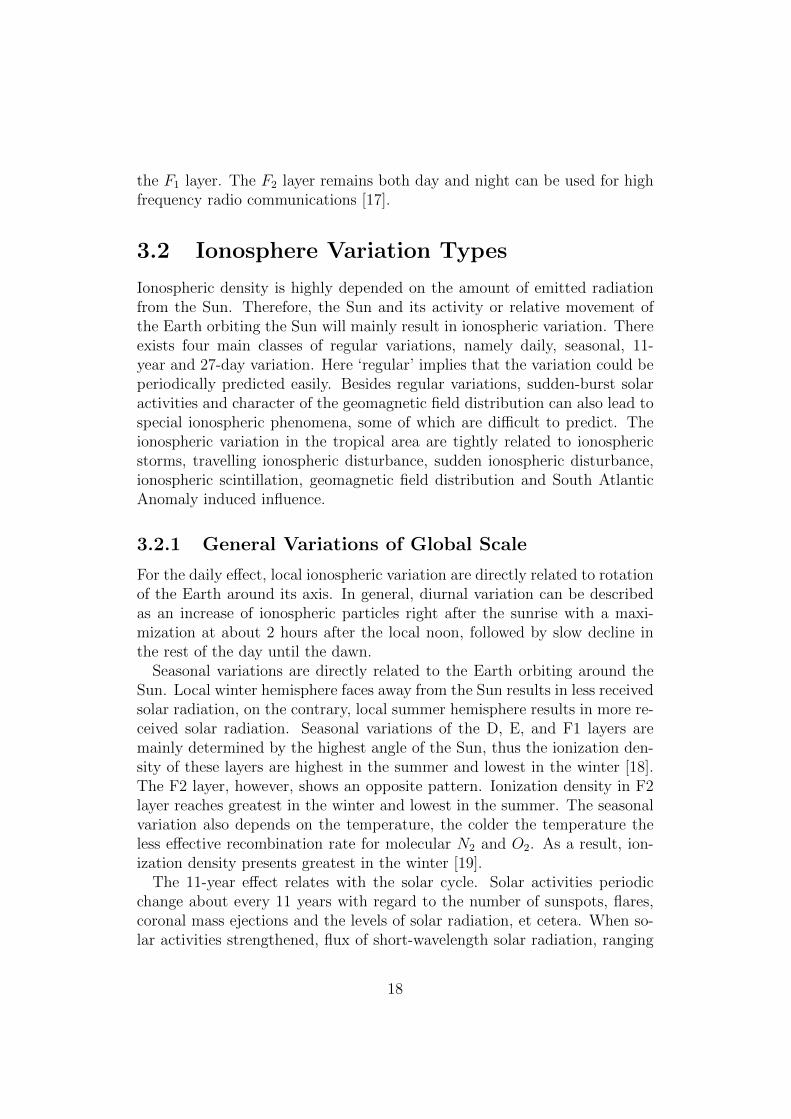
The South Atlantic Anomaly (SAA) results from the fact that the Earth’smagnetic field, the geographic center and poles are not perfectly aligned [31].The Earth is surrounded by a pair of concentric donut-shaped Van Allen ra-diation belts which trap and preserve charged particles from the solar winds.The geomagnetic field at the SAA is the weakest all over the world, seenfrom Figure 3.3, and the Earth’s inner Van Allen radiation belt at this re-gion comes closest to the Earth surface dropping down to an altitude ofabout 200 km [32]. The result is that, for a given altitude, higher-than-usuallevels of radiation can be found. Research has shown that greater TEC val-ues at local noon in the longitude sectors over and near the SAA have beenobserved [33]. Developed by European Space Agency (ESA), software ofSpace Environment Information System (SPENVIS) provides good modelsfor space environment analysis [34], a simulation, illustrated in Figure 3.4,shows that Brazil is mainly covered within the SAA region.
21
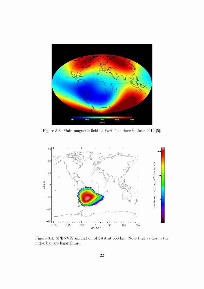
Figure 3.3: Main magnetic field at Earth’s surface in June 2014 [5].
Figure 3.4: SPENVIS simulation of SAA at 550 km. Note that values in theindex bar are logarithmic.
22
Chapter 4
Signal Propagation through theIonosphere
The mathematical expressions derived below follows from [1], [35–38]. Unlessotherwise indicated or cited clearly, most of the derivation can be done stepby step without too much difficulty.
4.1 Some Fundamentals of Wave Propagation
The relation between wavelength λ, the frequency f , and the propagationvelocity v is
v = λ · f (4.1)
Units for λ, f and v are meters (m), Hertz (Hz, oscillations per second), andmeters per second (m/s), respectively.
Relation between angular frequency ω and frequency f is
ω = 2πf (4.2)
The phase constant or wave number k can be expressed in terms of wave-length λ
k =2π
λ(4.3)
The wave propagation velocity v follows with expressions that
v = λ · f =λ
P=ω
k(4.4)
23

where P , reciprocal of the frequency, is the period of a wave.A periodic wave can be modeled by a sinusoidal function in space and
time.
y = Asin2π
(t
P+ Φ0
)(4.5)
where y is the magnitude at time t; Φ0 is the initial phase of the wave at tof 0, and A is the amplitude of the wave. The phase at time t is then
Φ =t
P+ Φ0 (4.6)
2πΦ is referred to phase angle φ. Inserting Equation (4.2) into Equation(4.5) has
y = Asin(ωt+ φ0) (4.7)
The relation between time, phase and frequency follows [1]
t =Φ
f(4.8)
Equation (4.8) gives a fundamental relation between the phase of a periodicwave and the corresponding time reading at the satellite clock, and can beconsidered to be the definition equation of a clock.
Propagation velocity, c, of an electromagnetic (EM) wave in a medium ofvacuum is
c =λvacP
= λvac · f =ω
kvac(4.9)
The propagation velocity in a non-vacuum medium is characterized by therefractive index n
n =c
v=λvacλ
=k
kvac(4.10)
The propagation velocity of the EM waves in a dispersive medium dependson the frequency. From Equation (4.10), it is easy to conclude that the indexof refraction (or refractivity) depends on the frequency or the wavelength ina dispersive medium.
The velocity dispersion is defined by
dv
dλ(4.11)
24

In a dispersive medium, different propagation velocities for sinusoidal wavesand groups of waves can be observed. Thus, concepts of phase velocity, vph,and group velocity, vgr, are introduced.
The phase velocity is the propagation velocity for a single EM wave withuniform wavelength and it is given by,
vph = λ · f (4.12)
For GPS, the carrier waves L1 and L2 are propagating with this velocity.The group velocity is the propagation velocity of a group of EM waves,
generated by a superposition of different waves with different frequencies. Itis given by
vgr = − dfdλλ2 (4.13)
According to [35]. This velocity has to be considered for GPS code measure-ments.
The relation between phase velocity and group velocity is described byRayleigh equation as
vgr = vph − λdvphdλ
(4.14)
Expressed in terms of the refraction index,
ngr = nph + fdn
df(4.15)
Derivation of Equation (4.14) and (4.15) can be found in [36].
4.2 Ionospheric Refraction
Propagation of radio signals within the ionosphere is primarily affected by‘free’ electrons and ions. Since the ionosphere is a dispersive medium withrespect to the GPS signal, refraction index of the phase can be expanded asa power series [1]
nph = 1 +c2
f 2+c3
f 3+c4
f 4+ ... (4.16)
The coefficient ci does not depend on the carrier frequency but on the quan-tity of electron density Ne along the propagation range. By dropping off the
25

series expansion terms above the quadratic order, the phase refractive indexis approximated as
nph = 1 +c2
f 2(4.17)
Differentiating above equation on both side gives
dnph = −2c2
f 3df (4.18)
Then, inserting Equation (4.17) and (4.18) into Equation (4.15) produces
ngr = 1− c2
f 2(4.19)
A comparison between Equation (4.17) and Equation (4.19) reveals that onlyan opposite sign exists for the group and the phase refractivity.
The formula of dispersion relates the refractive index n in an ionizedmedium with electron density Ne [37]
n = 1− neC2e2
πf 2me
(4.20)
where e is the elementary charge, me is the mass of an electron.An explicit derivation of index of refraction can be found in [38] as
n = 1− C ·Ne
f 2(4.21)
with C = 40.3. Equation (4.21) implies that the index of refraction is inverseproportional to the frequency squared. Reviewed from Equation (4.10), timedelay of a propagation signal relates with the index of refraction. Therefore,Equation (4.21) further indicates that signals with higher frequencies are lessinfluenced by the ionosphere.
The quadratic term coefficient of c2 can be estimated from Equation (4.21)to be
c2 = −40.3Ne [Hz2] (4.22)
Therefore, phase refractive index holds as
nph = 1− 40.3Ne
f 2(4.23)
26

Equation (4.23) indicates that a rough correction can be made for the delayin signal propagation if the an a priori electron density is known. Similarly,group refractive index holds as
ngr = 1 +40.3Ne
f 2(4.24)
Combining the relationship of ngr > nph with non-negative electron densityNe gives vgr < vph. As a result, the group and the phase velocity are delayedand advanced, respectively. In other words, GPS code measurements aredelayed and the carrier waves’ phases are advanced.
To quantitatively describe the ionosphere of the Earth, the TEC is used. Itis defined as the total number of electrons integrated between the receiver rand the satellite s, along a column with a cross section of one meter squared[36]. Mathematical expression is
TEC =
∫ s
r
Ne(l)dl (4.25)
where Ne(l) denotes the varying electron density along the integration path.Usually, the TEC is measured in TEC units (TECU) where
1 TECU = 1016 electron per m2 (4.26)
RE
EU
IPP
S
hion
Figure 4.1: Ionospheric single layermodel illustration, redrawn from [1].
Usually, the vertical total electroncontent (VTEC) is used instead ofthe slant TEC (STEC) for comparisonamong sets of TEC data. The relationbetween the VTEC and STEC are nor-mally expressed using a mapping func-tion.
A common used model is known asthe single layer model, see Figure 4.1.In this model it is assumed that allfree electrons are compressed in a thinspherical shell at a given height hion(usually in a range between 300 and400 km). The point of intersection be-tween the signal path and the layeris referred to as the ionospheric piercepoint (IPP). Zenith angle, α, is the an-gle spanned cross the signal path anda line extended from the center of the
27

Earth to the IPP. The relation between the VTEC, STEC, the elevation an-gle E, the given height hion and the radius of the Earth RE can be found inEquation (4.27) and (4.28) [36]
V TEC = STEC · cosα (4.27)
where the zenith angle
α = arcsin
(RE
RE + hioncosE
)(4.28)
The signal delay due to the ionosphere, denoted as dion [m], is given bythe difference between the actual signal path and the geometrical distancebetween the satellite and the receiver
dion =
∫ s
r
npds0 −∫ s
r
ds0 =
∫ s
r
(np − 1)ds0 (4.29)
Note that the true geometric range along a straight path between the satelliteand the receiver can be obtained from the subtrahend item.
The phase refractive index nph from Equations (4.23) yields the phase delayas
dion,ph =
∫ s
r
(1− 40.3Ne
f 2
)ds−
∫ s
r
ds0 (4.30)
The group refractive index ngr from Equation (4.24) yields the group delayas
dion,gr =
∫ s
r
(1 +
40.3Ne
f 2
)ds−
∫ s
r
ds0 (4.31)
Both the phase delay and the group delay equations can be further sim-plified by integrating the first term along the geometric straight path ds0.Review the TEC definition and substitute it into the phase and group delay,
dion,ph = −40.3 · TECf 2
and dion,gr =40.3 · TEC
f 2(4.32)
For LOS situation as shown in Figure 4.1, the zenith angle must be takeninto account because the propagation path range in ionosphere varies withan altering zenith angle. By introducing the zenith angle term, the phasedelay and the group delay can be modified to
dion,ph = − 1
cosα
40.3 · V TECf 2
and dion,gr =1
cosα
40.3 · V TECf 2
(4.33)
28

Only a difference in sign with respect to the above two expressions. Ex-tracting the common components
dion =1
cosα
40.3
f 2V TEC (4.34)
Such notation helps to omit the subscripts of ‘ph’ or ‘gr’ by taking the correctmodels. It implies that the ionospheric influence for the code pseudo-rangemeasurement is modeled by +dion and for the phase by −dion.
29

Chapter 5
Methodology of Obtaining theIonospheric Variability
Ionospheric phenomena like plasma bubbles would result in scintillation whichis thought to be primarily responsible for GPS signal distortion of phase andamplitude. Other direct consequences like loss of lock on GPS receivers andavailable GPS satellite number decrement can further limit the GPS trackingperformance and degrade the navigational accuracy. Therefore, to analyzethe temporal and spatial distribution of the plasma bubbles in Brazil is avery important issue.
The ionospheric effects can be studied by the dual-frequency ionospheremeasuring model. The difference between the L1 and L2 carrier frequencyof the GPS signal forms a so called L4-combination which could removeall frequency independent components. Recall the phase observable modeldiscussed in Chapter 2.5. A simple differential combination of both phasepseudo-ranges can be formed as [11]
λl1Φl1 − λl2Φl2 = ρp(fl1)− ρp(fl2) + λl1N1 − λl2N2 + λl1µl1 − λl2µl2 (5.1)
where Φl1 and Φl2 are the L1 and L2 phase pseudo-ranges (in units of cy-cles), ρp(fl1) and ρp(fl2) are ionospheric effects on the phase for the L1 andL2 carriers, N1 and N2 refer to the phase ambiguities of the L1 and L2 car-riers, µl1 and µl2 include signal multi-path and receiver measurement noisefor both carriers. The satellite L1-L2 biases are in common considered tobe constant in a few hours. Variation of the receiver inter frequency biasesis considered to be relatively small at constant receiver temperatures [39].Thus, both the satellite L1-L2 biases and the receiver inter frequency biasescontribution can be omitted here. Offset term of λl1N1−λl2N2 due to phaseambiguities remains constant, as long as no cycle slips occur which indicatea continuous of phase measurement. Consequently, an expression for the
30

Obs.1 Obs.2Mid.Obs.
SilentIonosphere
FluctuatingIonosphere
GPS Signals
δ1
Δ2
δ2Δm
Δ1
Figure 5.1: An illustration of linear interpolation.
slant ionospheric delay variations containing only error sources from signalmulti-path and measurement noise is achieved.
A simple exaggerated illustration of how interpolated value and measureddelay value could be applied to reflect the local ionospheric variation is shownin Figure 5.1, where only direction along the longitude is considered. Threeobservatories, namely observatory 1, middle observatory, and observatory 2,are equally spaced. As altitude of the GPS satellites are far more greaterthan the distance between adjacent observatories, green colored GPS sig-nals, emitted from the same satellite, can assumed to be parallel receivedby the three sites. Here, only the ionospheric delays are considered. Delayscaused by all frequency independent effects such as geometrical satellite-to-receiver distance and signal delay in the troposphere can be removed by theL4-combination. While, delays caused by other effects such as the inter fre-quency biases, phase ambiguity, signal multi-path and so on are omitted hereto simplify the discussion.
First, let us consider an ideal case where the ionosphere remains no fluctu-ation, corresponding to the blue line in the Figure 5.1. Only features of longwavelengths are present in this case. In this case, the middle site sees themean of the ionospheric delays of sites 1 and 2. In other words, the differencebetween measured ionospheric delay at the middle observatory (denoted as∆m) and expected ionospheric delay interpolated from other two observato-ries (denoted as ∆1 and ∆2) is zero.
Next, let us consider the case where the ionosphere no longer keeps still-ness. At a certain moment, all the three sites see a fluctuating ionosphere,
31

corresponding to red curve in the Figure 5.1. At this snapshot moment, as-sumed that the middle observatory see the slant ionospheric delay the sameas that of the none fluctuation case, however, the other two observatoriesclearly see different ionospheric delays greatly influenced by the undulatingionosphere. Here the notation of δ1 and δ2 merely imply a decrease and anincrease amount of ionosphere density, respectively. Meanwhile, comparedto the ionospheric delay under the none-fluctuation case, decrement iono-sphere density seen by the observatory 1 leads to a shorter ionospheric delay,whereas increment ionosphere density seen by the observatory 2 leads toa longer ionospheric delay. Therefore, the difference between the measuredionospheric delay at the middle observatory and the expected ionospheric de-lay interpolated from the other two observatories can not be zero any more.In other words, the difference contains information about the variability ofthe electron content at the observatory 1 and 2 right at that snapshot mo-ment. If many snapshot moments are involved, variability of the electroncontent distribution can be further acquired.
According to [40], in real application, the L4-combination is applied forthe three surrounding sites at the vertices of the triangular observationalnetwork to interpolate an estimated L4 value for the inner site. The in-terpolation is performed via bilinear interpolation along both latitude andlongitude direction. The bilinear interpolation is just an extension of linearinterpolation on a two dimensional grid scale. The weighted term of each sitecan be determined during the bilinear interpolation procedure as long as lat-itude and longitude components of each sites are known in advance. Further,the difference between the interpolated value and the measured L4 value atthe inner site are computed. For comparison purpose, it is reasonable toscale the difference into the zenith direction. This procedure is taken for allobserved satellites in order to obtain a distribution of the ionospheric varia-tion. Because the differences can yield both positive and negative outcomes,it makes sense to use the hourly root-mean-squared (rms) values. Finally,the obtained rms values are converted into the TEC units for analysis andcomparison.
The ionospheric spatial variability due to short wave term at the local smallscale is here denoted as swTEC, in order to differentiate from the long waveinduced TEC values estimated by data set of the IGS Ionosphere WorkingGroup. Both the swTEC and TEC have the same units, denoted as TECU.Note that the contributions from the multi-path and measurement noise canfurther be eliminated using a model presented in [41]. Detailed descriptionabout the methodology was referenced from [40] and can be read at AppendixA.
32

Chapter 6
Data Set
Data sets utilized in this project mainly includes observational data fromBrazilian ground stations, navigation data from the GPS satellites and globalVTEC maps data from the IGS Ionosphere Working Group.
Original observational data set can be downloaded directly from the offi-cial website of Brazilian Institute of Geography and Statistics or IBGE (Por-tuguese: Instituto Brasileiro de Geografia e Estatstica), as it provides obser-vational information within Brazilian territory. The selected ground stationsare distributed around geographical coordinates of 50◦ West and 22.5◦ South.They are divided into two triangular observational networks surrounding oneadditional station each to measure the L4-combination. Figure 6.1 shows theeight observational sites. Represented by blue dots, all sites are located in thesouthern part of Brazil where the ground GPS receiver network is relativelydense. Triangular network 1 includes surrounding stations of ILHA, ROSA,OURI with PPTE as the centering station. Triangular network 2 includessurrounding stations of SPBO, SPJA, MGIN with EESC as the centeringstation. The triangular network 2 located east of the triangular network 1is relatively smaller in scale. Such spatial difference can be visible in thecharacteristics of the local swTEC variation, discussed in next chapter.
Basically, observational data recorded each Thursday are chosen for awhole 2013 year study. Occasionally data are missing from one or moresites in the network. Therefore, data collected one day before or after thedata-missing-Thursday are selected instead. Detail information about whichdate’s data are chosen for both triangular networks are listed in AppendixB.
The format of the observational data has to be converted for further anal-ysis. The first-hand downloaded observational data have type name of com-pressed (zipped) folder, i.e., extension of ‘zip’. After decompression two typeof files can be acquired, one with type of ‘13N’, the other with ‘13O’. Here
33

only the files with ‘13O’ are preserved for further MATLAB analysis. Next,the ‘13O’ files are converted to ‘Text’ files via a batch program.
The daily satellite navigation messages come from the GPS broadcastephemeris data (BRDC) files. And they can be found from the websiteof NASA’s Archive of Space Geodesy Data. One advantage of the BRDCfile lies in that it is one navigation file offered by worldwide individual obser-vational stations and has already been merged into the non-redundant dailyGPS broadcast ephemeris which can be exploited by users rather than themultiple complex individual navigation files.
The merged BRDC file has a format of ‘brdcDDD0.YYn.Z’, where the
EESC
ILHA
MGINOURI
PPTEROSA SPBO
SPJA
−20
−10
−65 −60 −55 −50 −45 −40lon
lat
Figure 6.1: Map of the eight selected Brazilian observational sites.
three digits of ‘D’ and two digits of ‘Y’ are denoted for days and year, re-
34
spectively; ‘n’ indicates the satellite navigation information; ‘Z’ refers to thecompact format. Here take one example, a file name of ‘brdc0160.10n.Z’means that this navigation file is dedicated for navigation information of the16th day of the year 2010.
Before imported into MATLAB, file format conversion needs to be per-formed for those original downloaded navigation files. First step is to per-form a decompression operation. As a result, files with type of ‘13N’ aregenerated. Next step is to convert the ‘13N’ files into ‘Text’ files, which canbe realized by a simple batch program.
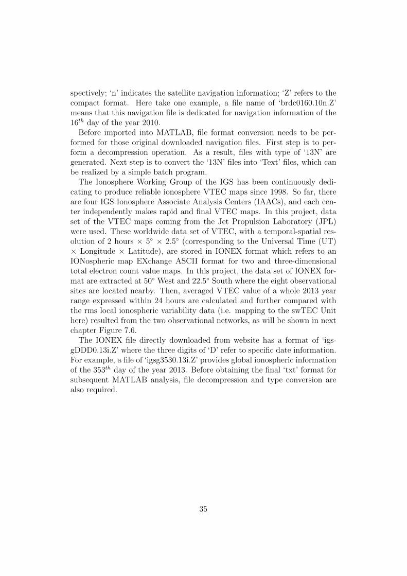
The Ionosphere Working Group of the IGS has been continuously dedi-cating to produce reliable ionosphere VTEC maps since 1998. So far, thereare four IGS Ionosphere Associate Analysis Centers (IAACs), and each cen-ter independently makes rapid and final VTEC maps. In this project, dataset of the VTEC maps coming from the Jet Propulsion Laboratory (JPL)were used. These worldwide data set of VTEC, with a temporal-spatial res-olution of 2 hours × 5◦ × 2.5◦ (corresponding to the Universal Time (UT)× Longitude × Latitude), are stored in IONEX format which refers to anIONospheric map EXchange ASCII format for two and three-dimensionaltotal electron count value maps. In this project, the data set of IONEX for-mat are extracted at 50◦ West and 22.5◦ South where the eight observationalsites are located nearby. Then, averaged VTEC value of a whole 2013 yearrange expressed within 24 hours are calculated and further compared withthe rms local ionospheric variability data (i.e. mapping to the swTEC Unithere) resulted from the two observational networks, as will be shown in nextchapter Figure 7.6.
The IONEX file directly downloaded from website has a format of ‘igs-gDDD0.13i.Z’ where the three digits of ‘D’ refer to specific date information.For example, a file of ‘igsg3530.13i.Z’ provides global ionospheric informationof the 353th day of the year 2013. Before obtaining the final ‘txt’ format forsubsequent MATLAB analysis, file decompression and type conversion arealso required.
35

Chapter 7
Results and Discussion
7.1 swTEC Analysis
Ionospheric variability of the two triangular observational networks in termsof swTEC TECU for a whole year range of 2013 is shown in Figure 7.1.These swTEC values are converted from the rms delay differences calculatedfrom the bilinear interpolation and the measured L4-combination value ateach inner site. Note that the swTEC amount of the observational network1 and 2 are colored by blue and red, respectively.
Both observational networks exhibit a similar tendency regarding the iono-spheric variation. The swTEC amount of both networks show high valuesfrom October to March (corresponding to Spring and Summer of the South-ern Hemisphere). Yet relative small swTEC values exist in the rest of theyear. This notable seasonal discrepancy of the ionospheric variation mainlyrelates to the seasonal solar radiation due to the Earth orbiting around theSun. Intense solar radiation flux in Spring and Summer can result in moreactive production of the ionospheric plasma irregularities or bubbles. Re-search has shown that activities of the plasma bubbles take place primarilyfrom September to March in Brazil [42]. Therefore, presence or absence ofthe plasma bubble activities throughout the year can be used to interpretthe ionospheric variation tendency shown in Figure 7.1.
The two observational networks show a relatively clear difference re-garding ionospheric variation. The swTEC variations of the observationalnetwork 1 is generally higher than the network 2. In other words, beingthe same selected days, observational network 1 generally presents higherswTEC value than that of the observational network 2. For example, thereare several days in Figure 7.1 that the swTEC are over 6 units for the obser-vational network 1, whereas no swTEC value are greater than 6 units for the
36

0 42 84 126 168 210 252 294 3360
1
2
3
4
5
6
7
8
9
10
Days
sw
TE
C (
TE
CU
)Whole year swTEC comparison
Network of PPTE,ILHA,ROSA,OURI
Network of SPBO,SPJA,EESC,MGIN
Figure 7.1: Local ionospheric variability comparison for the two observationalnetworks of a whole 2013 year.
observational network 2. This can be more obviously viewed from histogramplot in Figure 7.2. In addition, median value for both observational networksare calculated and compared.
Possible reason for this small-scale inhomogeneities is thought to be mainlyrelate to the spatial filtering effect. The relative larger spatial scale of theobservational network 1 indicates a less high-pass filtering ability in spatialas compared to that of the observational network 2. Thus, more fluctuationsof swTEC can be seen for the observational network 1. Whether such localswTEC variations are significantly different at different locations in Brazilrequires a consequent study with more observational networks involved.
The MSTIDs have been observed over low altitude range (220-300 km) inthe Brazilian territory. Features of the MSTIDs in Brazil have been summa-rized in research paper [43], from which a seasonal behavior of the MSTIDsshows a peak occurrence rate during the local Brazilian Winter time. Inaddition, most of the occurrences are observed during solar minimum yearswhereas no events are optically recorded during solar maximum. Therefore,
37

0 2 4 6 8 100
200
400
600
800
1000
TECU
Num
bers
Histogram plot of the first observational network
0 1 2 3 4 5 60
200
400
600
800
1000
TECU
Num
bers
Histogram plot of the second observational network
Figure 7.2: Histogram plot showing the occurrence frequency of the swTECunit. Median value: 1.4392 (top) and 0.9677 (below).
the MSTIDs could possibly be one contribution source for the swTEC varia-tion, especially during the local Winter period in solar minimum conditions.However, the swTEC contribution due to the MSTIDs as well as backgroundnoise can only result in small variation units which can be confirmed fromsmall variations of the local Winter part in the Figure 7.1 for both observa-tional networks.
Whether other ionospheric phenomenon such as the ionospheric stormsor the SIDs have inconvenient influence on the swTEC still needs furtherverification. Because both the ionospheric storms and SIDs are closely re-lated to the solar flare activities, correlation study can be made between theswTEC and records of the solar flare variation to further reveal how muchcontribution are coming from the solar flare activities.
38
7.2 Correlation Study
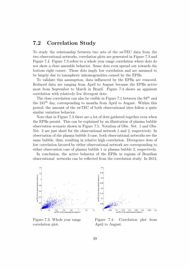
To study the relationship between two sets of the swTEC data from thetwo observational networks, correlation plots are generated in Figure 7.3 andFigure 7.4. Figure 7.3 refers to a whole year range correlation where dots donot show a close assemble behavior. Some dots even spread out towards thebottom right corner. Those dots imply low correlation and are assumed tobe largely due to ionospheric inhomogeneities caused by the EPBs.
To validate this assumption, data influenced by the EPBs are removed.Reduced data are ranging from April to August because the EPBs activemost from September to March in Brazil. Figure 7.4 shows an apparentcorrelation with relatively few divergent dots.
The close correlation can also be visible in Figure 7.1 between the 94th andthe 241th day, corresponding to months from April to August. Within thisperiod, the amount of the swTEC of both observational sites follow a quitesimilar variation behavior.
Note that in Figure 7.3 there are a lot of dots gathered together even whenthe EPBs persist. This can be explained by an illustration of plasma bubbleobservation scenario shown in Figure 7.5. Notation of Obs. Net. 1 and Obs.Net. 2 are just short for the observational network 1 and 2, respectively. Inobservation of the plasma bubble 3 case, both observational networks see thesame bubble, thus, resulting in relative high correlation. Divergence dots oflow correlation favored by either observational network are corresponding toeither observation case of plasma bubble 1 or plasma bubble 2, respectively.
In conclusion, the active behavior of the EPBs in regions of Brazilianobservational networks can be reflected from the correlation study. In 2013,
0 0.2 0.4 0.6 0.8 1 1.2 1.40
0.2
0.4
0.6
0.8
1
1.2
1.4
swTEC of the observational network 1
sw
TE
C o
f th
e o
bserv
ational netw
ork
2
Figure 7.3: Whole year rangecorrelation plot.
0 0.05 0.1 0.15 0.2 0.25 0.3 0.35 0.40
0.05
0.1
0.15
0.2
0.25
0.3
0.35
0.4
swTEC of the observational network 1
sw
TE
C o
f th
e o
bserv
ational netw
ork
2
Figure 7.4: Correlation plot fromApril to August.
39

Obs.Net.1
Plasma Bubble 3
Plasma Bubble 1Plasma Bubble 2
Obs.Net.2
Figure 7.5: Illustration of plasma bubble observation.
non-active period of the EPBs roughly starts from the middle of April untilthe end of August.
7.3 Comparison of TEC and swTEC
Expressed within a 24-hours time interval, the whole year TEC and swTECvariation are compared and illustrated in Figure 7.6. The TEC amount esti-mated from data set of the IGS Ionosphere Working Group, plotting in greencurve, can be read from the right Y-axis, while the swTEC amount estimatedfrom data set of the two local observational networks can be read from theleft Y-axis. Differences between these two estimations are quite obvious.
The evaluation of the TEC curve shown in Figure 7.6 is fairly straightfor-ward. The amount of the TEC begins to increase right after the local sunriseeach day until it reaches its maximum about two hours after the middaywhen the ionized electron density also reaches its daily maximum. After-wards, the amount of the TEC begins to decay continually until to the dawnof the next day. This 24-hours TEC variation explicitly agree with the factthat the ionization increases the amount of electron during the day, whileprevailing recombination declines the amount of electron during the night.
The behavior of the local swTEC variation for both observational net-works, however, show a different tendency where the amount of the swTECbegins to quickly climb up after about 19 o’clock at local time. Then, peakvalues are reached for both observational networks at vicinity of the localmidnight. Followed by a decay phase lasts until about two hours after the lo-
40

0 5 10 15 20 25
0.5
1
1.5
2
2.5
3
3.5
sw
TE
C (
TE
CU
)
Hours
Ionospheric Variability comparison of TEC and swTEC
0 5 10 15 20 25
10
20
30
40
50
60
70
TE
C (
TE
CU
)
TEC
swTEC of the network 1
swTEC of the network 2
Figure 7.6: Whole year TEC and swTEC comparison.
cal sunrise. The amount of the local swTEC remains relatively steady withinthe whole morning. Small increases are visible during the afternoon for bothobservational networks until to the local sunset. Main reason for such kindof the swTEC behavior is thought to relate to the generation and vanishmentof the EPBs during the night time.
The growth phase of the EPBs begins at approximate one to two hoursafter the local sunset at or near the geomagnetic equator. Then, the EPBsextend to low latitudes along the geomagnetic field lines due to pressuregradients. Around the local pre-midnight (one to two hours before the lo-cal midnight), the bubbles become gradually diluted and usually move tothe east. The two observational networks are not located at the geomag-netic equator but beyond 20 degrees south of the geomagnetic latitude (seefrom Figure 3.2). As the plasma bubbles move along the magnetic field linestowards low latitude regions, the plasma density accumulation results in con-centration gradient which also points to the low latitudes [27]. Such plasmadiffusion takes some time to arrive the region where the two observationalnetworks located. Therefore, it makes sense that the crest of the plasma
41

bubbles is observed at the time slightly before the local midnight.From the Figure 7.6 both the swTEC curves fluctuate within two TECU.
Another possible contribution may involve the MSTIDs which are usually ob-served with amplitudes of about one TECU. The spatial scale of the MSTIDscharacterized by hundred of kilometers also matches the scale of the two tri-angular observational networks. However, the extent of the MSTIDs con-tributing to the swTEC in the observational regions still requires furtheranalysis.
Similarly, the LSTIDs may contribute for the green colored TEC values.Research has reported that the amplitude associated with the LSTIDs canbe observed greater than 10 TECU during strong magnetic storms [44]. InBrazilian ionospheric variability case, intense day time ionization combineswith tropical ionospheric phenomena, for instance the daytime scintillations,as well as influence of the geomagnetic field distribution and the SAA. Thesephenomena can together pull up the TECU, far greater than those valuescalculated from the mid-latitude or high-latitude areas. Therefore, it maynot surprise to see relative large TEC amount obtained in Brazilian areafrom data set of the IGS Ionosphere Working Group. However, to what ex-tent could the LSTIDs contribute to the TEC amount still requires furtherinvestigation.
It should be pointed out that the local swTEC evaluation has superior tem-poral and spatial resolution. It has mentioned in previous data set chapterthat the IGS VTEC maps are sampled with 2 hours in time by 5◦ in longitudeand 2.5◦ in latitude, which maybe sufficient for a global TEC investigation.However, the IGS VTEC maps do not contain enough resolution for the localswTEC variation study. Therefore, less accuracy can be introduced regardingthe local small-scale TEC variation evaluation done by the IGS IonosphereWorking Group’s data set. In other words, the bilinear interpolation methodused by both the triangular observational networks performs a better localsmall-scale TEC variability computation than those VTEC maps producedfrom data set of the IGS Ionosphere Working Group.
It is obvious that in Figure 7.6, the swTEC amount of the two obser-vational networks are quite small compared to the TEC amount in a largedimensional scale. This is due to the spacial high-pass filtering effect on thetrue electron density variations from where the small-scaled highly fluctu-ation parts of the ionospheric variability can be captured by the two localobservational networks. Illustration of spacial high-pass filtering effect isshown in Figure 7.7. The blue colored oscillation curve corresponds to spa-cial high frequency terms of the ionospheric variability, whereas the blackcolored varying curve corresponds to the spacial low frequency terms of theionospheric variability in a relative large scale dimension. In other words, the
42

Figure 7.7: Spacial high-pass filtering effect can be resolved by the localobservational network.
small-scaled ionospheric variability due to activities of the EPBs can be re-solved and recorded by the local observational network, while the large-scaledvariation can be reflected from the data of IGS VTEC map.
7.4 Conclusion
This project presents a whole year ionospheric variability study at local sitesin Southern part of Brazil. The analysis has been performed for two nearbyobservational networks with spatial scale of hundred kilometers, matchingwith the spacial scale of the plasma bubbles which are normally of 100 kilo-meters in dimension. Results of the analysis show that the whole year iono-spheric variation tendency is strongly affected by the annual active periodof the EPBs from September to March. Daily behavior of the local swTECvariability has tight connection with the emergence and vanishment of theEPBs during the night time. Compared to the VTEC map data offered bythe IGS Ionosphere Working Group, the methodology applied in this projectyields fine local results for the small scale ionospheric variability. Because thelocal ionospheric variation details can be resolved by the spatial high-passfiltering effect performed by the observational networks.
43

7.5 Future Work
Future work may include several aspects of improvement:1). Due to sudden bursts of the tropical ionospheric irregularities, the
data sampled each Thursday may have lost some useful ionospheric variationinformation. Thus, perform a ‘truely’ whole year rms delay error analysis(then converted to TECU) including successive days may reveal some morefeatures.
2). Select more triangular observational networks to track the the localvariation of the ionospheric intensity. Further ground stations may comefrom the eastern regions of Brazil. Thus, traces of the plasma bubbles canbe studied in detail.
3). Integrate other GNSS receivers with the Russian GLONASS (Glob-alnaya Navigazionnaya Sputnikovaya Sistema) signal enabled can providesupplement for those lost observational data records. GNSS signals from theEuropean GALILEO system can offer a better resolution.
4). The IGS Ionosphere Working Group plan to reduce the temporalinterval from 2 hours to 1 hour in the near future, thus chose data with finetemporal-spatial resolution provided by the IGS Ionosphere Working Groupcan produce a better global VTEC map in Brazil.
5). Try to find a method to separate the ionospheric variation made bythe EPBs and the MSTIDs or other equatorial ionospheric phenomena andfind out to what extent these phenomena can contribute to the ionospherevariation.
6). A correlation study can be performed between the swTEC and thesolar flare variation to further reveal how much of TECU can be contributedfrom the solar flare activities.
44

References
[1] G. Seeber, Mathematik : Satellite Geodesy : Foundations, Methods, andApplications, ch. 2,7, pp. 44,54,212,220,235. Berlin: Walter de Gruyter,2nd ed., October 2008.
[2] P. Enge and F. van Diggelen, “GPS: An Introduction to SatelliteNavigation, With an Interactive Worldwide Laboratory Using Smart-phones.” https://class.coursera.org/gpslab-001, November 2014.Retrieved September 17, 2015.
[3] A. El-Rabbany, Introduction to GPS: The Global Positioning System.Artech House, 2nd ed., August 2006.
[4] National Geospatial-Intelligence Agency, “Maps of Magnetic Ele-ments from the WMM2015.” https://www.ngdc.noaa.gov/geomag/
WMM/image.shtml, May 2015. Retrieved October 8, 2015.
[5] ESA, “June 2014 Magnetic Field.” http://www.esa.int/
spaceinimages/Images/2014/06/June_2014_magnetic_field, June2014. Retrieved September 17, 2015.
[6] Wikipedia, “GPS Signals.” http://en.wikipedia.org/wiki/GPS_
signals#Navigation_message, November 2014. Retrieved April 17,2015.
[7] E. D. Kaplan and C. Hegarty, Understanding GPS: Principles and Appli-cations. Artech House Mobile Communications, Artech House, 2nd ed.,November 2006.
[8] U.S. Naval Observatory, “USNO NAVSTAR Global Positioning Sys-tem.” http://www.usno.navy.mil/USNO/time/gps/gps-info. Re-trieved April 16, 2015.
[9] J. Johansson, “Lecture Notes of Satellite Positioning,” tech. rep.,Chalmers University of Technology, November 2010.
45

[10] M. S. Grewal, L. R. Weill, and A. P. Andrews, Global Positioning Sys-tems, Inertial Navigation, and Integration. John Wiley & Sons.
[11] G. Xu, GPS Theory, Algorithms and Applications, ch. 4,5, pp. 37,41,51.Springer, 2007.
[12] A. Leick, GPS Satellite Surveying. New York: John Wiley, 1st ed., 1995.
[13] R. B. Langley, “Dilution of Precision.” http://www.nrem.iastate.
edu/class/assets/nrem446_546/week3/Dilution_of_Precision.
pdf, May 1999. Retrieved September 23, 2015.
[14] National Earth Science Teachers Association, “The Iono-sphere.” http://www.windows2universe.org/earth/Atmosphere/
ionosphere.html, 2012. Retrieved March 23, 2015.
[15] Wikipedia, “Ionosphere.” https://en.wikipedia.org/wiki/
Ionosphere, October 2015. Retrieved November 1, 2015.
[16] J. K. Hargreaves, The Upper Atmosphere and Solar-Terrestrial Rela-tions. Cambridge University Press, 3rd ed., May 1992.
[17] LUXORION Project, “Ionospheric Perturbations.” http://www.
astrosurf.com/luxorion/qsl-perturbation.htm. Retrieved October10, 2015.
[18] Integrated Publishing, “Variations In The Ionosphere.” http://www.
tpub.com/neets/book10/40h.htm. Retrieved October 19, 2015.
[19] S. Skone, “Lecture Notes of ENGO 633,” tech. rep., University of Cal-gary, 2007.
[20] M. J. Buonsanto, “Ionospheric Storms – A Review,” Space Science Re-views, vol. 88, pp. 563–601, March 1999.
[21] X. Pi, “Ionospheric Storms.” http://iono.jpl.nasa.gov/storm.
html. Retrieved March 19, 2015.
[22] A. Coster and T. Tsugawa, “The Impact of Traveling Ionospheric Dis-turbances on Global Navigation Satellite System Services .” http://
www.ursi.org/proceedings/procga08/papers/fgp1.pdf. RetrievedOctober 13, 2015.
[23] Z. T. Katamzi and L.-A. McKinnell, “Observations of Traveling Iono-spheric Disturbances Associated with Geomagnetic Storms,” IEEE 2011XXXth URSI General Assembly and Scientific Symposium, 2011.
46

[24] Y. Memarzadeh, Ionospheric Modeling for Precise GNSS Applications.PhD thesis, Netherlands Geodetic Commision, 2009.
[25] National Oceanic and Atmospheric Administration, “Sudden Iono-spheric Disturbance (SID).” http://www.ngdc.noaa.gov/stp/
space-weather/ionospheric-data/sids/documentation/readme_
sudden-ionospheric-disturbances.pdf, March 2014. RetrievedOctober 13, 2015.
[26] IPS Radio and Space Services, Bureau of Meteorology, AustralianGovernment, “About Ionospheric Scintillation.” http://www.sws.bom.
gov.au/Satellite/6/3. Retrieved March 21, 2015.
[27] M. A. Hei, R. A. Heelis, and J. P. McClure, “Seasonal and Longitu-dinal Variation of Large-scale Topside Equatorial Plasma Depletions,”Journal of Geophysical Research - Space Physics, vol. 110, December2005.
[28] D. Shvarts, U. Alon1, D. Ofer, R. L. McCrory, and C. P. Verdon, “Non-linear Evolution of Multi-mode Rayleigh–Taylor Instability in Two andThree Dimensions,” in Proceedings of the Fifth International Workshopon Compressible Turbulent Mixing, World Scientific, 1996.
[29] A. Taori, J. J. Makela, and M. Taylor, “Mesospheric Wave Signaturesand Equatorial Plasma Bubbles: A Case Study,” Journal of GeophysicalResearch: Space Physics (1978-2012), vol. 115, June 2010.
[30] M. C. Kelley, J. J. Makela, O. de La Beaujardire, and J. Retterer, “Con-vective Ionospheric Storms: A Review,” Reviews of Geophysics, vol. 49,pp. 445–446, June 2011.
[31] Mori, “The South Atlantic Anomaly.” http://www.
bibliotecapleyades.net/ciencia/ciencia_earthchanges49.htm,November 2007. Retrieved June 1, 2015.
[32] E. Stassinopoulos, “Forty–Year Drift and Change of The SAA,” tech.rep., NASA Goddard Spaceflight Center, 2007.
[33] A. Kapusta, A. J. Coster, and P. J. Erickson, “The South AtlanticAnomaly and Its Influence on The Total Electron Content Distribution,”American Geophysical Union, Fall Meeting 2006, December 2006.
[34] M. Kruglanski, E. D. Donder, N. Messios, L. H. Emmanuel Gamby,and S. Calders, “SPENVIS Homepage.” www.spenvis.oma.be/, Octo-ber 2013. Retrieved March 17, 2015.
47

[35] M. Bauer, Vermessung und Ortung mit Satelliten. Wichmann, 3rdedn. ed., 1994.
[36] B. Hofmann-Wellenhof, H. Lichtenegger, and J. Collins, Global Posi-tioning System: Theory and Practice, ch. 6, pp. 97–98,102. Springer,5th revised ed., 2001.
[37] K. Davies, Ionospheric Radio. IEEE Electromagnetic Waves Series 31,London: Peter Peregrinus, 1990.
[38] L. R. Hartmann, G., “Range Errors Due to Ionospheric and Tropo-spheric Effects for Signal Frequencies Above 100 MHz,” Bull. Geod.,vol. 58, pp. 109–136, 1984.
[39] C. Rieck, P. Jarlemark, K. Jaldehag, and J. Johansson, “Thermal Influ-ence on the Receiver Chain of GPS Carrier Phase Equipment for Timeand Frequency Transfer,” IEEE International Frequency Control Sym-posium and PDA Exhibition Jointly with the 17th European Frequencyand Time Forum, vol. 13, pp. 326–331, 2003.
[40] T. R. Emardson, P. O. J. Jarlemark, J. M. Johansson, and S. Schfer,“Spatial Variability In The Ionosphere Measured With GNSS Net-works,” Radio Science, vol. 48, pp. 646–652, 2013.
[41] R. Emardson, P. Jarlemark, S. Bergstrand, T. Nilsson, and J. M. Johans-son, “Measurement Accuracy In Network–RTK,” tech. rep., SP Boras,2009.
[42] L. F. C. de Rezende, E. R. de Paula, I. J. Kantor, and P. M. Kintner,“Mapping and Survey of Plasma Bubbles Over Brazilian Territory,”Journal of Navigation, vol. 60, pp. 69–81, 2007.
[43] D. C. M. Amorim, A. A. Pimenta, J. A. Bittencourt, and P. R. Fagundes,“Longterm Study of Medium-scale Traveling Ionospheric DisturbancesUsing O I 630 nm Allsky Imaging and Ionosonde Over Brazilian LowLatitudes,” Journal of Geophysical Research. A. Space Physics, vol. 116,2011.
[44] J. Jakobsen, Kinematic GNSS: Ionospheric Variations and Character-istics of Multipath. PhD thesis, University of Copenhagen, 2010.
[45] P. O. J. Jarlemark, T. R. Emardson, J. M. Johansson, and G. Elgered,“Ground–Based GPS for Validation of Climate Models: The Impactof Satellite Antenna Phase Center Variations,” IEEE Transactions onGeoscience and Remote Sensing, vol. 48, pp. 3847–3854, 2010.
48

Appendix A
Methodology for Estimatingthe Ionospheric Variability
The measurement of the small scale ionospheric spatial variability of swTEC,denoted as σ4l, is based on the deviation between interpolated and ‘true’measured ionospheric electron content, 4l, at the center of a triangular ob-servational network. The4l can be obtained by forming the L4-combinationvia the carrier phase measurement model and eliminating the non ionosphericcontributions.
According to the carrier phase measurement model, the phase observed bya single GPS receiver at L1 and L2 carrier can be modeled as:
ΦL1 =ρ
λL1
+NL1 + fL1(∆tsL1 + ∆trL1) +lL1i
λL1
+ltλL1
+ µL1 (A.1)
ΦL2 =ρ
λL2
+NL2 + fL2(∆tsL2 + ∆trL2) +lL2i
λL2
+ltλL2
+ µL2 (A.2)
where Φ is the measured phase in fraction of cycles; λ is the wavelength ofcarrier signal; ρ is the true geometrical satellite-to-receiver distance; N isthe phase ambiguity parameter which is the integer number of cycles; f isthe carrier frequency; ∆ts and ∆tr refer to the satellite and receiver clockbias respectively; li and lt refer to the signal delay in the ionosphere andtroposphere respectively; and µ contains the signal multi-path and receivermeasurement error.
By combining the above equations, a new expression, which removes allfrequency independent terms such as the geometrical distance (ρ) as well asthe signal delay in the troposphere (lt), is achieved.
λL1ΦL1 − λL2ΦL2 = lL1i − lL2
i + λL1NL1 − λL2NL2+C(∆tsL1 −∆tsL2 + ∆trL1 −∆trL2) + λL1µL1 − λL2µL2
(A.3)
I

where C refers to the speed of the light in vacuum. As can be seen inEquation (A.3), the difference regarding the ionospheric effect between thetwo frequencies is however produced. Thus this combination can be used toderive the TEC along the LOS propagation in the ionosphere.
Based on Equation (A.3), the slant ionospheric delay can be obtained. Areorganized form of equation shows
Θsp ≡ κ(λL1φ
L1 − λL2φL2) = Is + n+ τs + τr + µ (A.4)
where Is is the slant TEC and κ is the scaling factor between L4 measure-ments and the TEC. This derived L4-combination, Θs
p, contains informationabout the ionosphere but also potential non-ionospheric variations from themulti-path and measurement noise, µ; the receiver inter frequency L1-L2bias, τr; the satellite inter frequency L1-L2 bias, τs; and the phase ambigui-ties, n.
Two assumptions should be noted here. One is that the GPS receivers haveconstant temperatures, thus the receiver L1-L2 bias variation is consideredto be relatively small [39]. The satellite L1-L2 biases are generally consideredto be constant over several hours. The phase ambiguity term is by definitionconstant over satellite passes. Therefore, by applying the time average of Θs
p
over a satellite passage we can form a new variable with the time-averagedvalue removed containing only contributions from the ionosphere, I, as wellas the multi-path and measurement noise µ.
Θs = Θsp − a
{Θsp
}(A.5)
where the time averaged term
a{
Θsp
}= a {Is + n+ τs + τr + µ} = Ism + n+ τs + τr + µm (A.6)
The method during the analysis procedure is based on by using obser-vations of the slant ionospheric delay from the three sites in a triangularobservational network in order to interpolate the expected ionospheric de-lay for a site at the center. Therefore, for each site in a triangle the L4-combination for a specific satellite observation can be formed. By applyingthe L4-combination to each of the three surrounding sites at the vertices ofthe triangular network, an expected L4-combination at the inner site can beinterpolated. The interpolation is performed through bilinear interpolationalong both latitude and longitude components of plane coordinates. The dif-ference between the interpolated and measured L4 values, at the inner site,is calculated as
4Θs = Θs −Θsi (A.7)
II

where
Θsi =
3∑n=1
anΘsn,
3∑n=1
an = 1 (A.8)
The weights of an can be uniquely determined during the bilinear interpola-tion as long as both the latitude and longitude components of each site areknown in advance. And n just refers to the three surrounding sites.
The next step followed is to map the L4 deviations to the zenith direction,
Θ =Θs
mi(ε)(A.9)
where mi is the mapping function
mi(ε) =R + h√
(R + h)2 −R2cos2ε(A.10)
and ε is the observational elevation angle; R is the radius of the earth and h isthe height of the ionosphere, usually between ranges of 300 km and 400 km,represented as a thin shell. The interpolation operation and the mapping tothe zenith result in a 4Θ containing the seeking ionospheric electron contentdeviation 4l.
Now all available 4Θ values from all visible satellites during one hour canbe employed to construct the hourly rms values. To guarantee continuity ofthe integer number of cycles in the measured carrier phase, only cycle slipfree satellites with passage time longer than 1 hour are utilized. In orderto receive LOS GPS signals, satellite observation elevation angle above 20◦
are chosen. In fact, the duration of the satellite passes we use is typically acouple of hours in this project.
σ4Θ =
√∑ 4Θ2
N(A.11)
This rms value contains contribution from the ionosphere, I, and the multi-path and measurement noise, µ. Since these contributions can be assumedto be uncorrelated, a squared term of swTEC can be written as
σ24l = σ2
4Θ − σ24µ (A.12)
The expected contribution from the multi-path and measurement noisecan be removed according to a model discussed in [41] and [45].
Last, the ionospheric variability σ4l can be obtained from Equation (A.12).
III

Appendix B
Observational Data Set
This part describes how the observational data were selected from the IGBEwebsite. For the during of year 2013, 155 days’ data are used in this investiga-tion. Basically, data of each Thursday were used to produce the ionosphericvariation. Specifics regarding the data can be found in Table B.1.
According to calendar of the year 2013, the first Thursday should be Jan-uary 3rd, however, station of MGIN lost data on that day. The same stationalso lost data the following day. Therefore, the 5th day was chosen to repre-sent the first week data.
Data sampled every 7 days go smoothly from 10th day (second Thursday)to 52th day. Then, instead of the 59th day, the 60th day was selected. Thisis because at the very beginning we downloaded the observational data fromthe NASA website instead of the IBGE website and there was no observa-tional data record for the ILHA station at the 59th day in NASA website,thus the next day was chosen. When we realized the downloading error we
Table B.1: Specific date used from IBGE website each Thursday
Date
5th 10th 17th 24th 31th 38th 45th 52th
60th 66th 73th 80th 87th 94th 101th 108th
115th 122th 129th 136th 143th 150th 157th 164th
171th 178th 185th 192th 199th 206th 213th 220th
227th 234th 241th 248th 255th 262th 269th 274th
283th 290th 297th 304th 311th 318th 325th 331th
339th 346th 353th 360th
IV

still decided to use the navigation file of the 60th day, but selected the ob-servational data from the IBGE website. Data of the 60th day leads to anunexpected outcome because this specific day yielded large rms delay differ-ences which imply strong local ionospheric variability occurred (see ‘Result’chapter Figure 7.1).
Next, data sampled every 7 days go smoothly from 66th day to 360th day,the last Thursday (26 of December). Specific data lost are:
(1) Missing data for the SPJA station at 276th day. Same happened at275th day for this station, therefore, data of 274th day was selected instead.
(2) Missing data for the ILHA station at 332th day, thus data of 331th daywas used instead.
Besides data sampled every 7 days through the whole year, another twotwo-months-datasets were collected and processed for supplementary pur-pose. One dataset starts from the 30th day to the 89th day with a missingdata at the 61th day (at this time, data set of the 59th day were included).Another starts from the 283th day to the 346th day with a missing data atthe 332th day. Both missing data result in discontinuities (need to zoom into see clearly) in the plot of Figure 7.1.
V