IPS9 in R: Bootstrap Methods and Permutation Tests(Chapter 16)

Bonnie Lin and Nicholas Horton (nhorton@amherst.edu)July 22, 2018

Introduction and background

These documents are intended to help describe how to undertake analyses introduced as examples in theNinth Edition of Introduction to the Practice of Statistics (2017) by Moore, McCabe, and Craig.

More information about the book can be found here. The data used in these documents can be found underData Sets in the Student Site. This file as well as the associated R Markdown reproducible analysis sourcefile used to create it can be found at https://nhorton.people.amherst.edu/ips9/.

This work leverages initiatives undertaken by Project MOSAIC (http://www.mosaic-web.org), an NSF-fundedeffort to improve the teaching of statistics, calculus, science and computing in the undergraduate curriculum.In particular, we utilize the mosaic package, which was written to simplify the use of R for introductorystatistics courses. A short summary of the R needed to teach introductory statistics can be found in themosaic package vignettes (http://cran.r-project.org/web/packages/mosaic). A paper describing the mosaicapproach was published in the R Journal: https://journal.r-project.org/archive/2017/RJ-2017-024.

For those less familiar with resampling, the mosaic resampling vignette may be a useful additional reference(https://cran.r-project.org/web/packages/mosaic/vignettes/Resampling.pdf).

Chapter 1: Looking at data – distributions

This file replicates the analyses from the (online-only) Chapter 16: Bootstrap Methods and PermutationTests.

First, load the packages that will be needed for this document:library(mosaic)library(readr)

Section 16.1: The bootstrap idea

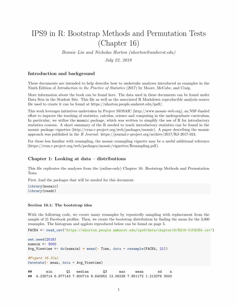
With the following code, we create many resamples by repeatedly sampling with replacement from thesample of 21 Facebook profiles. Then, we create the bootstrap distribution by finding the mean for the 3,000resamples. The histogram and qqplots reproduced below can be found on page 5.FACE4 <- read_csv("https://nhorton.people.amherst.edu/ips9/data/chapter16/EG16-01FACE4.csv")

set.seed(2018)numsim <- 3000Avg_Viewtime <- do(numsim) * mean(~ Time, data = resample(FACE4, 21))

#Figure 16.3(a)favstats(~ mean, data = Avg_Viewtime)

## min Q1 median Q3 max mean sd n## 4.235714 6.977143 7.800714 8.640952 13.06238 7.851172 1.213376 3000

1

## missing## 0

gf_histogram(~ mean, data = Avg_Viewtime) %>%gf_labs(x = "Mean time of resamples (in minutes)", y = "Count")

0

100

200

300

4 6 8 10 12

Mean time of resamples (in minutes)

Cou

nt

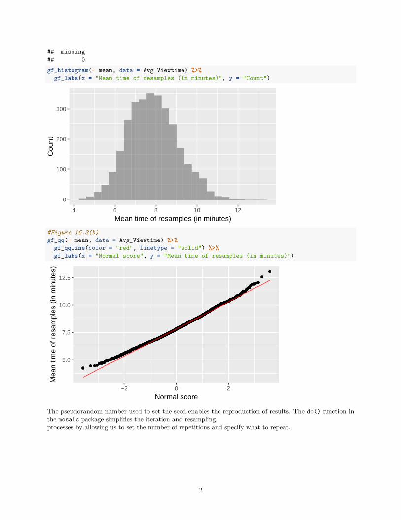
#Figure 16.3(b)gf_qq(~ mean, data = Avg_Viewtime) %>%

gf_qqline(color = "red", linetype = "solid") %>%gf_labs(x = "Normal score", y = "Mean time of resamples (in minutes)")

5.0

7.5

10.0

12.5

−2 0 2

Normal score

Mea

n tim

e of

res

ampl

es (

in m

inut

es)

The pseudorandom number used to set the seed enables the reproduction of results. The do() function inthe mosaic package simplifies the iteration and resamplingprocesses by allowing us to set the number of repetitions and specify what to repeat.

2

Section 16.2: First steps in using the bootstrap

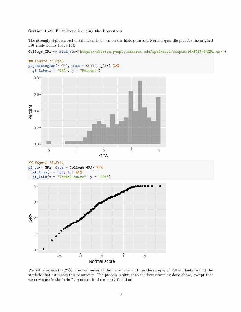
The strongly right skewed distribution is shown on the histogram and Normal quantile plot for the original150 grade points (page 14):College_GPA <- read_csv("https://nhorton.people.amherst.edu/ips9/data/chapter16/EG16-04GPA.csv")

## Figure 16.8(a)gf_dhistogram(~ GPA, data = College_GPA) %>%

gf_labs(x = "GPA", y = "Percent")

0.0

0.2

0.4

0.6

0.8

0 1 2 3 4

GPA

Per

cent

## Figure 16.8(b)gf_qq(~ GPA, data = College_GPA) %>%

gf_lims(y = c(0, 4)) %>%gf_labs(x = "Normal score", y = "GPA")

0

1

2

3

4

−2 −1 0 1 2

Normal score

GPA

We will now use the 25% trimmed mean as the parameter and use the sample of 150 students to find thestatistic that estimates this parameter. The process is similar to the bootstrapping done above, except thatwe now specify the “trim” argument in the mean() function:

3

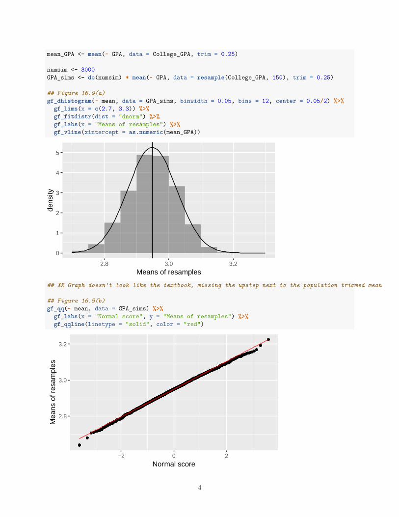
mean_GPA <- mean(~ GPA, data = College_GPA, trim = 0.25)

numsim <- 3000GPA_sims <- do(numsim) * mean(~ GPA, data = resample(College_GPA, 150), trim = 0.25)

## Figure 16.9(a)gf_dhistogram(~ mean, data = GPA_sims, binwidth = 0.05, bins = 12, center = 0.05/2) %>%

gf_lims(x = c(2.7, 3.3)) %>%gf_fitdistr(dist = "dnorm") %>%gf_labs(x = "Means of resamples") %>%gf_vline(xintercept = as.numeric(mean_GPA))

0

1

2

3

4

5

2.8 3.0 3.2

Means of resamples

dens

ity

## XX Graph doesn't look like the textbook, missing the upstep next to the population trimmed mean

## Figure 16.9(b)gf_qq(~ mean, data = GPA_sims) %>%

gf_labs(x = "Normal score", y = "Means of resamples") %>%gf_qqline(linetype = "solid", color = "red")

2.8

3.0

3.2

−2 0 2

Normal score

Mea

ns o

f res

ampl

es

4

## XX Graph doesn't look like the textbook one, missing outliers

Since the seed has been previously set, we do not need to set the seed in this code chunk again.

To find the 95% confidence interval for the population trimmed mean as the book does on page 16, we cantype:confint(GPA_sims, level = 0.95)

## name lower upper level method estimate## 1 mean 2.791954 3.091326 0.95 percentile 2.949605

## XX The textbook reports 2.794, 3.106 and the standard error is 0.078.## Now wondering if the GPA_sims is the right data

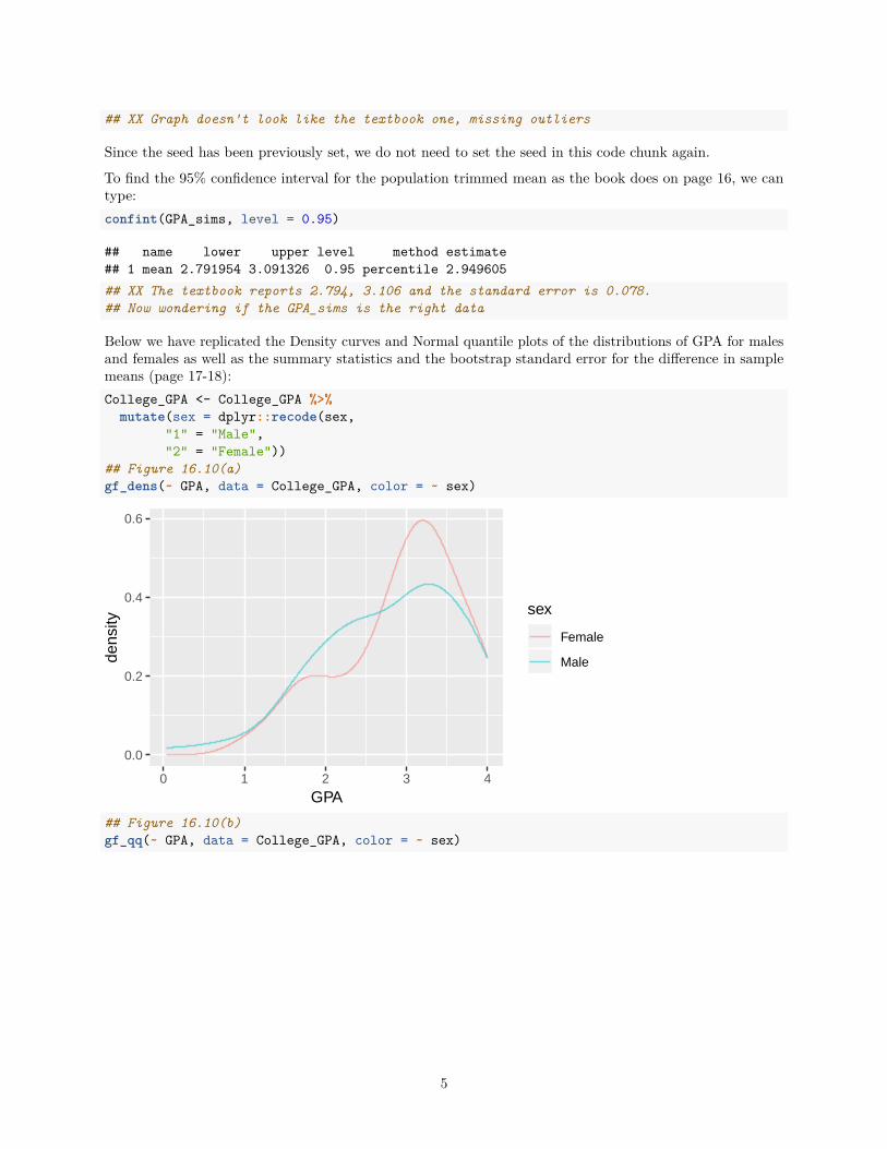
Below we have replicated the Density curves and Normal quantile plots of the distributions of GPA for malesand females as well as the summary statistics and the bootstrap standard error for the difference in samplemeans (page 17-18):College_GPA <- College_GPA %>%

mutate(sex = dplyr::recode(sex,"1" = "Male","2" = "Female"))

## Figure 16.10(a)gf_dens(~ GPA, data = College_GPA, color = ~ sex)

0.0

0.2

0.4

0.6

0 1 2 3 4

GPA

dens

ity

sex

Female

Male

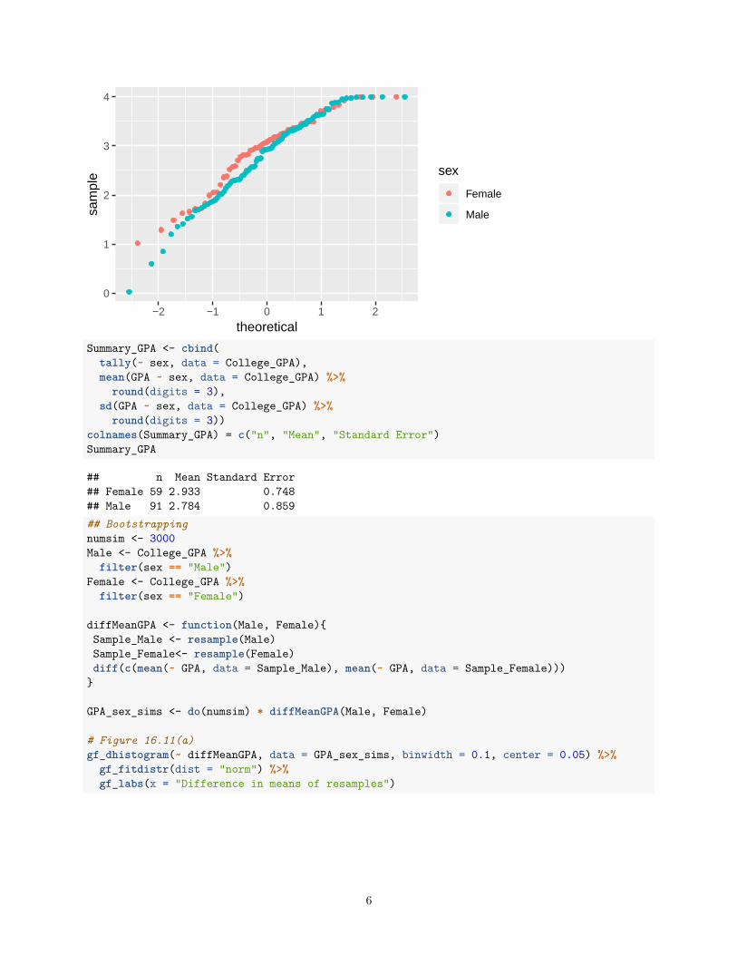
## Figure 16.10(b)gf_qq(~ GPA, data = College_GPA, color = ~ sex)

5

0

1

2

3

4

−2 −1 0 1 2

theoretical

sam

ple sex

Female

Male

Summary_GPA <- cbind(tally(~ sex, data = College_GPA),mean(GPA ~ sex, data = College_GPA) %>%

round(digits = 3),sd(GPA ~ sex, data = College_GPA) %>%

round(digits = 3))colnames(Summary_GPA) = c("n", "Mean", "Standard Error")Summary_GPA

## n Mean Standard Error## Female 59 2.933 0.748## Male 91 2.784 0.859

## Bootstrappingnumsim <- 3000Male <- College_GPA %>%

filter(sex == "Male")Female <- College_GPA %>%

filter(sex == "Female")

diffMeanGPA <- function(Male, Female){Sample_Male <- resample(Male)Sample_Female<- resample(Female)diff(c(mean(~ GPA, data = Sample_Male), mean(~ GPA, data = Sample_Female)))

}

GPA_sex_sims <- do(numsim) * diffMeanGPA(Male, Female)

# Figure 16.11(a)gf_dhistogram(~ diffMeanGPA, data = GPA_sex_sims, binwidth = 0.1, center = 0.05) %>%

gf_fitdistr(dist = "norm") %>%gf_labs(x = "Difference in means of resamples")

6

0

1

2

3

−0.4 −0.2 0.0 0.2 0.4 0.6

Difference in means of resamples

dens

ity

# Figure 16.11(b)gf_qq(~ diffMeanGPA, data = GPA_sex_sims) %>%

gf_labs(x = "Normal score", y = "Difference in means of resamples") %>%gf_qqline(linetype = "solid", color = "red")

−0.2

0.0

0.2

0.4

0.6

−2 0 2

Normal score

Diff

eren

ce in

mea

ns o

f res

ampl

es

We resample separatelyfrom the two samples, so that each of our 3000 resamples consists of two group resamples, one of size91 drawn with replacement from the male data and one of size 59 drawn with replacement from the femaledata.

XX No data for Example 16.7 (page 20) “Do all daily numbers have an equal payoff”

Section 16.3: How accurate is a bootstrap distribution?

Section 16.4: Bootstrap confidence intervals

Up to this point, we have demonstrated the use of the bootstrap to find confidence intervals of the samplemean, trimmed mean, and the difference between two means.

Now we will bootstrap the confidence intervals for the correlation coefficient, as introduced on page 35.

7

LAUND24 <- read_csv("https://nhorton.people.amherst.edu/ips9/data/chapter16/EG16-10LAUND24.csv")

# Figure 16.19gf_point(Rating ~ PricePerLoad, data = LAUND24)

30

40

50

60

10 20 30

PricePerLoad

Rat

ing

# Figure 16.20(a)numsim <- 5000cor_LAUND24 <- cor(Rating ~ PricePerLoad, data = LAUND24)LAUND_sims <- do(numsim) * cor(Rating ~ PricePerLoad, data = resample(LAUND24))gf_dhistogram( ~ cor, data = LAUND_sims, binwidth = 0.05, center = 0.025) %>%

gf_fitdistr(dist = "dnorm") %>%gf_labs(x = "Correlation coefficient of resamples") %>%gf_vline(xintercept = cor_LAUND24)

0

1

2

3

4

0.4 0.6 0.8

Correlation coefficient of resamples

dens

ity

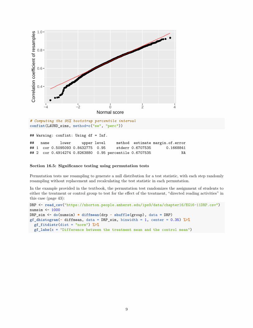
# Figure 16.20(b)gf_qq(~ cor, data = LAUND_sims) %>%

gf_labs(x = "Normal score", y = "Correlation coefficient of resamples") %>%gf_qqline(linetype = "solid", color = "red")

8

0.4

0.6

0.8

1.0

−4 −2 0 2 4

Normal score

Cor

rela

tion

coef

ficie

nt o

f res

ampl

es

# Computing the 95% bootstrap percentile intervalconfint(LAUND_sims, method=c("se", "perc"))

## Warning: confint: Using df = Inf.

## name lower upper level method estimate margin.of.error## 1 cor 0.5095093 0.8432775 0.95 stderr 0.6707535 0.1668841## 2 cor 0.4914274 0.8263880 0.95 percentile 0.6707535 NA

Section 16.5: Significance testing using permutation tests

Permutation tests use resampling to generate a null distribution for a test statistic, with each step randomlyresampling without replacement and recalculating the test statistic in each permutation.

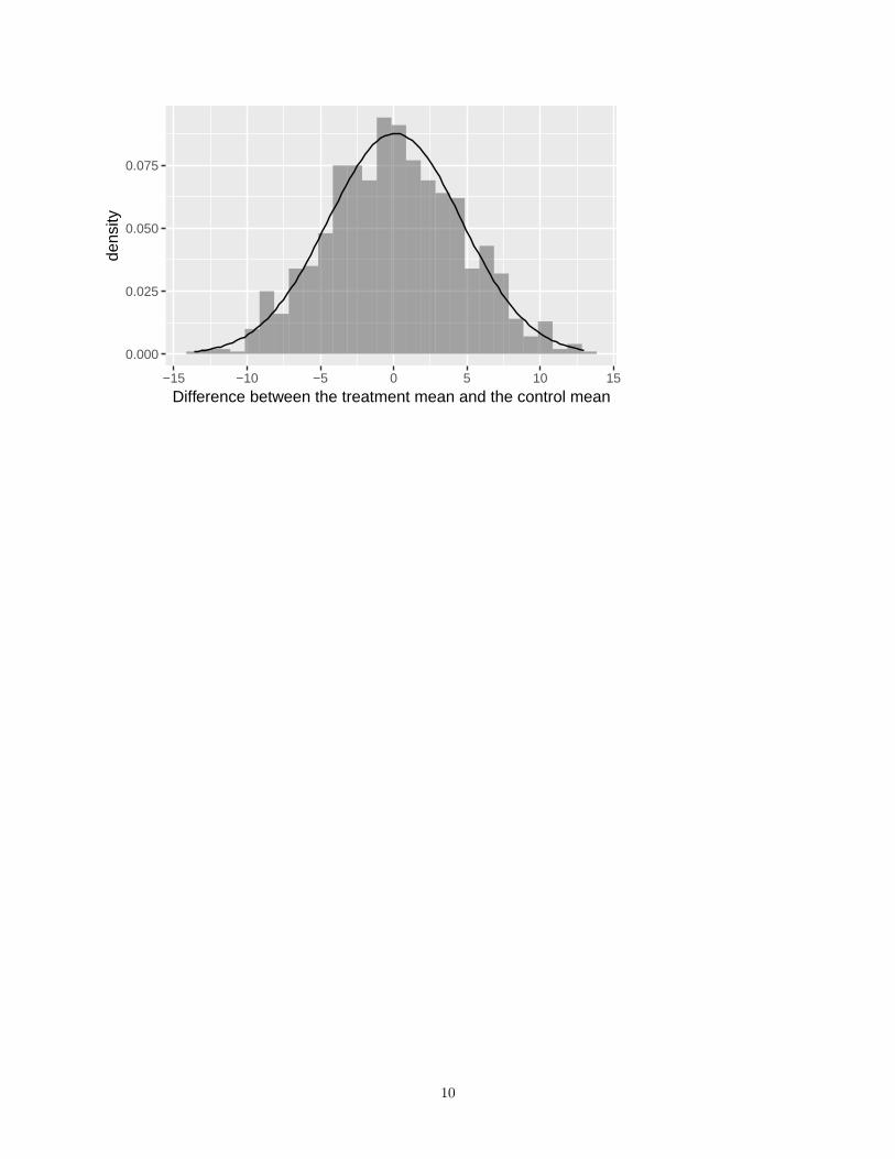
In the example provided in the textbook, the permutation test randomizes the assignment of students toeither the treatment or control group to test for the effect of the treatment, “directed reading activities” inthis case (page 43):DRP <- read_csv("https://nhorton.people.amherst.edu/ips9/data/chapter16/EG16-11DRP.csv")numsim <- 1000DRP_sim <- do(numsim) * diffmean(drp ~ shuffle(group), data = DRP)gf_dhistogram(~ diffmean, data = DRP_sim, binwidth = 1, center = 0.35) %>%

gf_fitdistr(dist = "norm") %>%gf_labs(x = "Difference between the treatment mean and the control mean")

9

0.000

0.025

0.050

0.075

−15 −10 −5 0 5 10 15

Difference between the treatment mean and the control mean

dens

ity

10