iron fertilization in the ocean and consequences for the ... fertilization in the ocean and...

Iron fertilization in the ocean and consequences for theglobal carbon cycle

Eric-Martial Takam Takougang ([email protected])African Institute for Mathematical Sciences (AIMS)

Supervised by Irina MarinovWoods Hole Oceanographic Institution (WHOI)

Co-supervised by Mark TadrossClimate System Analysis Group, University of Cape Town

May 24, 2007

Abstract

It has been suggested that fertilizing the ocean with iron can stop the continuing increase ofatmospheric carbon dioxide by enhancing the biological uptake of carbon. This would decreasethe surface ocean partial pressure of carbon dioxide, thus forcing the absorbtion of carbon dioxidefrom the atmosphere. Using a five-box model of the ocean circulation, we study the responseof the ocean due to iron fertilization and its consequences for the carbon dioxide atmosphericpartial pressure. We simulate the fertilization in the North Atlantic, the low latitudes and theSouthern Ocean, assuming a strong productivity in each area of experimentation. We find thatthe Southern Ocean is the most effective area for reducing atmospheric carbon dioxide, witha drop of 28 ppm in carbon dioxide atmospheric partial pressure after 150 years of continuousfertilization.

i

Contents

Abstract i

1 Introduction 1

2 Iron fertilization in the ocean 2

2.1 The ocean as the major CO2 container . . . . . . . . . . . . . . . . . . . . . . 2

2.1.1 The solubility pump . . . . . . . . . . . . . . . . . . . . . . . . . . . . 2

2.1.2 The biological pump . . . . . . . . . . . . . . . . . . . . . . . . . . . . 3

2.2 The role of iron . . . . . . . . . . . . . . . . . . . . . . . . . . . . . . . . . . 5

2.3 The concept of iron fertilization . . . . . . . . . . . . . . . . . . . . . . . . . . 7

2.3.1 A bit of history . . . . . . . . . . . . . . . . . . . . . . . . . . . . . . . 7

2.3.2 What is iron fertilization? . . . . . . . . . . . . . . . . . . . . . . . . . 8

2.4 Some iron fertilization experiments . . . . . . . . . . . . . . . . . . . . . . . . 8

3 Modeling the ocean circulation 10

3.1 Two-box model of the ocean carbon cycle . . . . . . . . . . . . . . . . . . . . 10

3.2 Three-box model of the ocean carbon cycle . . . . . . . . . . . . . . . . . . . . 12

3.3 Five-box model of the ocean carbon cycle . . . . . . . . . . . . . . . . . . . . . 15

4 Simulation of iron fertilization with a five-box model 20

4.1 Running the simulation . . . . . . . . . . . . . . . . . . . . . . . . . . . . . . 20

4.2 Discussion of the results . . . . . . . . . . . . . . . . . . . . . . . . . . . . . . 23

4.2.1 Fertilisation in the low latitude . . . . . . . . . . . . . . . . . . . . . . 23

4.2.2 Fertilization in the North Atlantic . . . . . . . . . . . . . . . . . . . . . 23

4.2.3 Fertilization in the Southern Ocean . . . . . . . . . . . . . . . . . . . . 25

4.3 Sensitivity studies of the ocean . . . . . . . . . . . . . . . . . . . . . . . . . . 26

5 Conclusion 30

Bibliography 33

ii

1. Introduction

In the aftermath of the industrial boom of the late nineteenth century, human activities such asfossil fuel burning, cement production and tropical deforestation have led to an increase in theemission of carbon dioxide into the atmosphere. An increase from 280 ± 10 ppm before theindustrial revolution to 373 ppm in 2002 has been observed[1], meaning a spectacular jump of 93± 10 ppm in less than 200 years. This jump is similar to that of the transition from the glacialto the interglacial period, with the difference that the glacial-interglacial changes occurred overhundred of thousands of years [1].

The growth of carbon dioxide in the atmosphere leads to an increase of the earth’s temperature,due to its nature as a greenhouse gas. It acts by trapping the reflected radiation from the earthand thus making the earth warmer. A direct consequence is the observed rising of the sea levelat an average rate of 1 to 2 mm/year over the past 100 years resulting from the melting oficebergs at high latitudes. This rise is significantly larger than the rate averaged over the lastseveral thousand years and causes several climatic problems like floods and hurricanes which bringdisaster to the population. The increase of the earth’s temperature and its consequences is calledglobal warming and constitutes a challenge for the scientific community of this century. It isnecessary to find a solution to this problem.

In the late 1980s, the oceanographer John Martin [2] showed the role of iron in boosting thephotosynthesis process at the ocean surface. The micro-organisms responsible are phytoplankton.They fix the dissolved carbon to form organic matter, thus forcing more carbon dioxide from theatmosphere to be trapped in the ocean. Martin suggested the possibility of sequestering enormousquantities of carbon dioxide from the atmosphere by seeding vast areas of open ocean with ironand thus decreasing the quantity of carbon dioxide in the atmosphere.

This revolutionary idea has gripped the attention of the scientific community as a possible solutionagainst global warming. Several experiments have been carried out, during which a bloom ofphytoplankton was observed, thereby confirming the effect of iron in boosting photosynthesis.However, due to the short time scale of those experiments (a few weeks), it was difficult toconclude anything about the drop of atmospheric carbon dioxide and its effect in the ocean afterseveral years of fertilization. Considering the time scale of the ocean circulation (the overturningcirculation of the ocean has a time scale of order 1000 years [3]), the best way to test this ideais perhaps by modelling.

Using a five-box model of the ocean circulation, we will simulate the fertilization experiment inthree areas of the sea surface: the North Atlantic, the low latitudes and the Southern Ocean.We will try to find the response of the ocean and of the atmospheric carbon dioxide after a fewhundred years of simulation. We compare the results in each fertilization zone to determine themost effective zone for sequestering CO2.

1

2. Iron fertilization in the ocean

2.1 The ocean as the major CO2 container

About 70% of the world’s surface is covered by oceans. Carbon dioxide is more present in theocean than in the atmosphere. Indeed, if we look at the pre-industrial ocean-atmosphere carbon,98.5% of the total CO2 is found in the ocean and only 1.5% in the atmosphere. By contrast, wefind only 0.6% of world’s oxygen in the ocean [4]. The reasons for the large amount of CO2 inthe oceans are its high solubility, (which is thirty times that of oxygen) [1], the chemical reactionsit undergoes with water to give carbonate and bicarbonate ions, and biochemical reactions withmicro-organisms in the sea. CO2 is a greenhouse gas which acts by trapping the reflected radiationfrom the Earth. The more CO2 trapped in the ocean, the colder the climate.

Observations show that the concentration of DIC (dissolved inorganic carbon) increases from thesurface to deep ocean. The DIC is the sum of the concentrations of CO2, bicarbonate (HCO−

3 )and carbonate (CO2−

3 ) ions:

DIC = [CO2] + [HCO−3 ] + [CO2−

3 ]. (2.1)

Carbon dioxide in the ocean undergoes the following reactions:

CO2 + H2O ⇔ H2CO3 ⇔ H+ + HCO−3 ⇔ 2H+ + CO2−

3 , (2.2)

which gives 88% of HCO−3 , 10.9% of CO2−

3 and only 0.5% of CO2 for the total DIC [1].

We have around 1970 umol1/kg of DIC at the surface and 2280 umol/kg in deep ocean [1], whichis approximately 12% lower at surface than at depth[4] [5]. This surface to deep difference is dueto the biological and the solubility pumps [5], which we shall now discuss

2.1.1 The solubility pump

The net transport of DIC from the surface to the deep ocean due to temperature and salinity iscalled the solubility pump. This mechanism is driven by two factors:

• The thermohaline circulation due to the formation of deep water at high latitudes where thewater is cooler and denser with high salinity. The thermohaline circulation is an overturningcirculation in which the warm water flows polewards and is subsequently converted into coolwater that sinks and flows towards the equator in the interior (see figure 2.1). In the NorthAtlantic, we have the North Atlantic Deep Water (NADW) which penetrates southwardat depths between 1500m and 2500m [1]. In the Southern Ocean we have the AntarcticBottom Water (AABW) which flows northwards into the Indian, Pacific and Atlantic basinsupwelling at 3500 m [6]. Radiocarbon measurements show that the thermohaline circulationturns over all the deep water in the ocean every 600 years [6] or 1000 years [3].

1One umol=10−6 mol

2

Section 2.1. The ocean as the major CO2 container Page 3

Figure 2.1: NASA schematic view of ocean circulation. The light shows the general movement ofthe surface water and the dark coloured path shows the movement of deep water. The numbersshow the position of: 1. The Gulf Stream, which transports heat from the tropics to northernEurope; 2. North Atlantic Deep Water formation which results from strong cooling; 3. AntarcticBottom Water formation due to sea ice production around Antarctica.

• The solubility of carbon dioxide is a strong inverse function of sea water temperature. Thismeans that carbon dioxide is more soluble at high latitudes which are cooler than at lowlatitudes. Consequently, at high latitudes the formation of deep water together with thehigher solubility of carbon dioxide results in the transportation of carbon dioxide from thesurface to the deep ocean.

2.1.2 The biological pump

The biological pump is a suite of biological processes that transport carbon from the surface zoneto the ocean’s interior. It includes the carbonate and the soft tissue pump:

• The carbonate pump is related to the formation of calcium carbonate CaCO3 from calcium(Ca2+) and carbonate ions (see equation 3.4) at the sunlit surface. Calcium carbonateforms the shells of micro-organisms living at the sea surface such as coccolithophores,foraminiferans or pteropods.

Ca2+ + CO2−3 ⇔ CaCO3 (2.3)

Calcium carbonate dissolves at a rate dependent upon local carbonate chemistry. As thisprocess is slower than the synthesis process, and because the particulate material is sinking,

Section 2.1. The ocean as the major CO2 container Page 4

the carbonate pump transports material from the surface of the ocean to its depths.

• The soft tissue pump transports the dissolved organic carbon formed by photosynthesis byphysical processes such as downwelling or sinking. Remineralization converts organic matterback into dissolved inorganic matter deep in the ocean. This leads to a net transport ofDIC from the surface to the depth (see figure 2.2).

Figure 2.2: The soft tissue pump: part of the organic matter produce by photosynthesis isremineralized at the surface, where CO2 returns back to the atmosphere, and another part sinksinto the ocean interior.

Photosynthesis is a process by which plants, phytoplankton and some bacteria use the energyfrom sunlight to produce glucose, with the release of oxygen. It is arguably the most importantbiochemical pathway known; nearly all life depends on it. The conversion of unusable sunlightenergy into usable chemical energy is associated with the action of the green pigment called

Section 2.2. The role of iron Page 5

chlorophyll. The equation of photosynthesis is:

6CO2 + 6H2O ⇔ C6H12O6 + 6O2, (2.4)

with C6H12O6 representing the organic matter.

The organisms responsible for photosynthesis at the ocean surface are phytoplankton. In additionto CO2 and water, they need nutrients such as phosphorus, nitrogen and iron to produce organicmatter. The reaction is presented as follows [7]:

↙ Fe106CO2 + 16HNO3 + H3PO4 + 78H2O ⇔ C106H75O42N16P + 150O2,

(2.5)

with nitrogen in the form of HNO3 and phosphorus in the form of H3PO4. The organic matterof composition C106H75O42N16P is built with a stoichiometric ratio of C, N, P and O2 as:C:N:P:O2 = 106:16:1:150[7]. The stoichiometric ratio between a suite of elements is the ratio ofthese elements in the organic matter. Recent research has expanded this ratio as: C:N:P:O2:Fe= 106:16:1:150:0.001. This means that each unit of iron can fix 106,000 units of carbon, 16,000units of nitrate and 1,000 units of phosphate.

The quantity of iron needed is very small compared to the quantity of phosphate or nitrate; butwithout iron, phytoplankton will not survive.

2.2 The role of iron

An observation of the annual phosphate as well as the annual nitrate (see figures 2.3 and 2.4) levelsat the ocean surface shows that these nutrients are not uniformly distributed. We have areas whereconcentrations of nitrate and phosphate are close to zero and others with high concentration. Theareas with the highest concentrations are the Southern Ocean and the Subarctic Pacific with 1.5to 2.0 umol/kg, followed by the Arctic zone with 1.0 umol/kg. Normally, we expect those regionsto be biologically very active and to have the highest population of plankton. Curiously, someof them have a very weak population of phytoplankton. This can be seen by observing figures2.3, 2.4 and 2.5 which shows that the Southern Ocean, the Surbarctic Pacific and the EquatorialPacific, all regions of high nutrients concentrations, are very poor in chlorophyll (pigmentationdue to photosynthesis carried by phytoplankton). Those regions are described as High NutrientsLow Chlorophyll (HNLC). The reason for this is the limited quantity of iron in these regions. Thisis due to the large distance between them and the large deserts (Kalahari, Sahara and Arabiandeserts) which consequently cannot supply enough iron as they do for the rest of the ocean [10].The North Atlantic is at the same latitude as the Subarctic Pacific but is supplied with quantitiesof iron dust from the Sahara desert in Africa. Consequently the North Atlantic is not an HNLCregion. Iron comes into the ocean in the form of dust transported by wind and plays a vital roleas a micronutrient for photosynthesis and the growth of phytoplankton.

Section 2.2. The role of iron Page 6

Figure 2.3: Observed annual mean phosphate concentration at the ocean surface in umol/kg [8]

Figure 2.4: Observed annual mean nitrate concentration at the ocean surface in umol/kg. Thisimage clearly shows the high levels of nitrate in the subarctic Pacific, the equatorial Pacific andthe Southern Ocean [8].

Section 2.3. The concept of iron fertilization Page 7

Figure 2.5: This chlorophyll map shows the concentration of chlorophyll in phytoplankton. Thepurple areas near the equator show low chlorophyll levels; yellow and brown areas indicate increasedlevels; and red indicates high levels. We can see the low level of chlorophyll in the Subarctic Pacific,the Equatorial Pacific and the Southern Ocean [9].

2.3 The concept of iron fertilization

The previous observation led to the idea that one could improve the growth of phytoplanktonby fertilizing the surface ocean with iron, and as a consequence, extract more CO2 from theatmosphere.

2.3.1 A bit of history

The oceanographer John Martin was the first to propose the idea of iron fertilization in orderto manage global warming when he declared in the late 1990s: “Give me half a tanker of ironand I’ll give you another ice age” [11] His studies indicated that it was indeed a scarcity ofiron micronutrients that was limiting phytoplankton growth in some area of the ocean like theSouthern Ocean. He also gave an explanation for the glacial-interglacial climate change as beingthe consequence of a bloom of phytoplankton due to higher concentration of iron dust in theocean. Martin hypothesized that restoring high levels of plankton photosynthesis could slow oreven reverse global warming by sequestering enormous volumes of CO2 in the Ocean [11].

A few months after the eruption of Mount Pinatudo in 1991 in the Philippines, the environmentalscientist Andrew Watson analysed global data from the eruption and calculated that it depositedapproximately 4 × 1010g of iron dust into the Southern Ocean [12]. The minerals were washed

Section 2.4. Some iron fertilization experiments Page 8

into the oceans, where the iron fertilized the plankton which enabled them to fix and metabolisemore CO2. This fertilization event generated an observed global increase of O2 and decline ofCO2 in the atmosphere [12], perhaps showing the evidence of Martin’s hypothesis.

2.3.2 What is iron fertilization?

As we said before, iron fertilization consists of adding iron to the upper ocean to enhance thegrowth of phytoplankton and, as a consequence, boost photosynthesis to fix more CO2 andslow down global warming. This CO2 contributes to the formation of organic matter which isexpected to sink to the deep ocean. In fact, just approximately 30% of this carbon-rich biomasssinks below 200 meters into the colder water strata below the thermocline [4]. Part of this fixedcarbon continues falling into the abyss and the rest is dissolved and remineralized. However at thisdepth, the carbon is suspended in the deep ocean and effectively isolated from the atmospherefor centuries. Most of this sinking happens at high latitudes because that is where the deep wateris formed.

NASA and NOAA estimate a decline of the phytoplankton population in the last 25 years ofat least 6%. Simply returning this population to its previous levels of health and activity couldtherefore annually sequester 2 to 3 billion more tons of CO2 than are being removed today.

Iron fertilization targets are areas that have persistently high levels of major nutrients, suchas nitrate and phosphate, but are also weakly photosynthetic (HNLC) regions. An importantexample is the Southern Ocean, which has the largest repository of unused macronutrients insurface water, and plays a key role in the formation of intermediate and deep water [13]. Theseareas might represent a non-negligible ratio of about 16% of the total surface ocean [14].

2.4 Some iron fertilization experiments

Some experiments have been performed to test the efficiency of iron fertilization. These experi-ments consisted of adding quantities of iron nutrients in the form of iron sulfate to some of theHNLC areas. For example,

• the SEEDS field experiments in the Western and Eastern subarctic North Pacific [15],

• the SERIES experiment in the Northeast Subarctic Pacific [16],

• the SOIREE experiment in the Polar Southern Ocean [13],

• the experiments in the Equatorial Pacific Ocean [17].

The majority of these experiments have resulted in the study of only the evolution phase of thebloom except in the Northeast Subarctic Pacific where an increase in POC (particulate organiccarbon) flux at 50 m depth has been observed [16]. All of these showed arguably the importanceof iron in boosting phytoplankton growth and the consequent fixation of more nutrient and CO2

Section 2.4. Some iron fertilization experiments Page 9

in the biomass at the ocean surface. However, little is known about the net effect on the air-seacarbon dioxide flux and atmospheric pCO2.

The scientific community is divided about the efficiency of iron fertilization. The entrepreneurMichaels [11] claims that he can cancel out the world contribution to atmospheric CO2 increasesfrom burning fossil fuel by fertilizing 16 million square miles of the Southern Ocean with 8.1million tons of iron [11]. Supporters of this idea also think that the growth of phytoplanktonpopulation will have a positive impact on the food chain by providing more food for other species.

On the other hand, some researchers think that this is not the best idea. As the populationof phytoplankton grow due to iron nutrient, other species like zooplankton grows also by eatingthe phytoplankton. Therefore, the biomass remains at the surface from where all the fixed CO2

returns back to the atmosphere following decomposition by bacteria. At present it is difficult topredict the consequences in the ocean ecology due to iron fertilization.

The previous experiments were performed in a relatively small area compared to the total surfaceof the ocean, typically ten by ten kilometers and usually lasting only few weeks . This makesprediction of the ocean response based on these experiments difficult.

In order to learn more, we will next model the carbon cycle in the context of simple box modelswith circulation. Our models are similar to the three-box model of Sarmiento and Toggweiler [3],or that of Siegenthaler and Wenk [5].

3. Modeling the ocean circulation

Phenomena such as the thermohaline and thermocline circulations, the Antarctic Bottom Wateras well as the North Atlantic Deep Water and the surface ocean movements driven by windssuch as the Gulf Stream, make the understanding and prediction of ocean features difficult. Oneattempt to study this is perhaps by modeling, providing that the model takes into considerationthe most importants characteristics of the ocean, depending on the research problem.

Restricting ourselves to iron fertilization experiments, a good model should take into considerationthe difference in concentration of DIC, PO3 and NO4 from the surface to the deep ocean. Thiscan be done by separating the ocean into boxes, each box representing a particular part of theocean. The simplest such model is a two-box model.

3.1 Two-box model of the ocean carbon cycle

In a two-box model, the ocean is divided into two parts: the surface and the deep ocean. Thisdivision is controlled by the difference in concentration of elements such as DIC, PO3 and NO4

which play a key role in the global carbon cycle. Observations show that the concentration ofthose elements increases from the surface to the deep ocean and is driven by two factors knownas the biological and solubility pumps (see section 2.1).

The model takes into account (figure 3.1) the net biological uptake from the surface to the deepocean and the mixing terms between the reservoirs.

Taking Vs and Vd to be respectively the volume of the surface and deep ocean in m3, DICs, O2s

and PO4s respectively the concentration of dissolved inorganic carbon, oxygen and phosphate atthe surface box in umol/m3 and finally DICd, O2s and PO4s respectively the dissolved inorganiccarbon, oxygen and phosphate at the deep box, we have:

1. In the surface box

The equations of time rate of change of DIC, PO4, O2 are:

VsdDICs

dt= υ(DICd −DICs)− FDIC + φCO2 ,

VsdO2s

dt= υ(O2d −O2s)− FO2 + φO2 ,

VsdPO4s

dt= υ(PO4d − PO4s)− FPO4 ,

(3.1)

with FDIC and FPO4 the biological sinks due to photosynthesis, φCO2 and φO2 respectivelythe net flux of carbon dioxide and oxygen into the ocean due to gas exchange with theatmosphere:

φCO2 = KβCO2(pCO2atm − pCO2ocean), (3.2)

10

Section 3.1. Two-box model of the ocean carbon cycle Page 11

Figure 3.1: Two-box model of the Ocean. F represents the net biological uptake from the surfaceto the deep box. K and υ in m3/s respectively represent the mixing term or vertical exchangerate between the surface box and the atmosphere and between the surface box and the deep box.

φO2 = KβO2(pO2atm − pO2ocean). (3.3)

pCO2atm, pO2atm, pCO2ocean and pO2ocean represent the partial pressure of carbon dioxideand oxygen in the atmosphere and in the ocean. βCO2 and βO2 are respectively the solubilityof carbon dioxide and oxygen in mol/m3 · atm.

2. In the deep box

The equations of time rate of change of DIC, PO4, O2 are:

VddDICd

dt= υ(DICs −DICd) + FDIC ,

VddPO4d

dt= υ(PO4s − PO4d) + FPO4 ,

VddO2d

dt= υ(O2s − PO2d) + FO2 .

(3.4)

Section 3.2. Three-box model of the ocean carbon cycle Page 12

At steady state, the system of equations 3.4 becomes the system of equations 3.5:υ(DICd −DICs) = FDIC ,

υ(PO4d − PO4s) = FPO4 ,

υ(O2d − PO2s) = FO2 .

(3.5)

DIC, PO4 and O2 are in stoichiometric ratio of C:P:O2=117:1:-170 [3] such that:

O2d −O2s = rP : O2 × (PO4d − PO4s), (3.6)

with rP:O2 the stoichiometric ratio between phosphate and oxygen. From equation 3.6 we canfind the concentration of oxygen in the deep ocean.

Taking O2s=234 mmol/m3, PO4d=2.1 mmol/m3 and using P:O2=-170 [1], we obtain:

O2d = 234− 170× (2.1− 0) (3.7)

= −123mmol/m3. (3.8)

This result (equation 3.7) is clearly wrong because it is impossible to have a negative concentrationof oxygen in the ocean. The conclusion is that our model is incorrect. Why?

We assumed that the concentration of nutrients is uniform at the ocean surface. This is incorrect,because at high latitudes we find much more unutilized nutrients, known as preformed nutrients[1] than at low latitudes. From figures 2.2 and 2.3 we observe that the concentration of phosphateand nitrate at high latitudes ranges from 1.5 to 2.0 umol/l , whereas in low-latitude oceans it isclose to zero. This difference is related to chemical and physical processes in which both regionsare involved. Additionally, the North Atlantic Deep Water (NADW) and the Antarctic BottomWater (AADW) currents driven by the thermohaline circulation (section 2.2), result in the surfaceto deep differences in oxygen, nutrients and DIC.

We then need to modify our model to consider the thermohaline circulation and the differencein nutrients between the low and high-latitude surface oceans. We divide the surface ocean intotwo regions (the low-latitudes and the high-latitudes), thus creating a three-box model.

3.2 Three-box model of the ocean carbon cycle

This model was described by Sarmiento and Toggweiller in 1984 [3] to show the importance ofthe thermohaline circulation and the high-latitude surface ocean in the decrease of carbon dioxideatmospheric partial pressure (pCO2) during the last ice age. From this model, Sarmiento andToggweiller suggested that the decrease of pCO2 during the last ice age was the response to anincrease in the net high-latitude productivity coupled with a possible decrease of the thermohalineoverturning.

The model (figure 3.2) is made up of:


1. a box representing the low-latitude surface ocean of thickness 100 m [3],

2. a box representing the high-latitude surface ocean, denser and cooler of thickness 250 m.It represents 16 % of the whole surface ocean,

3. a box representing the deep ocean to which all materials from the surface sink, and getremineralized after a certain period of time.

Figure 3.2: Three-box model of the ocean: Pl and Ph represent the sinking particle and dissolvedinorganic matter flux from the low latitudes and the high latitudes in mol/s. Kl and Kh arerespectively the gas exchange coefficient between the low-latitude surface and the atmosphereand between the high-latitude surface and the atmosphere. T is the thermohaline circulation andf is the vertical exchange rate between the high-latitude and the deep ocean in m3/s.

We consider that most of the interactions between the surface and the deep ocean in terms ofsolubility happen at the high latitudes.

Taking Vl, Vh and Vd to be respectively the volume of the low-latitude surface, high-latitudesurface and deep ocean in m3, φCO2l

, φO2l, φCO2h

are φO2hthe net flux of carbon dioxide and

oxygen into the ocean, due to gas exchange with the atmosphere at low and high latitudes, theequations of time rate of change of DIC, PO4, O2 are:

1. In the first box:


VldDICl

dt= −PlDIC + T (DICd −DICl) + φCO2l

,

VldO2l

dt= −PlO2 + T (O2d −O2l) + φO2l

,

VldPO4l

dt= −PlPO4 + T (POd − POl).

(3.9)

2. In the second box:

VhdDICh

dt= f(DICd −DICh) + T (DICl −DICh)

−PhDIC + φCO2h,

VhdO2h

dt= f(O2d −O2h) + T (O2l −O2h)

−PhO2 + φO2h,

VhdPO4h

dt= f(PO4d − PO4h) + T (POl − POh)− PhPO4 .

(3.10)

3. In the third box

VddDICd

dt= (T + f)(DICh −DICd) + PhDIC + PlDIC ,

VddO2d

dt= (T + f)(O2h −O2d) + PhO2 + PlO2 ,

VddPO4d

dt= (T + f)(PO4h − PO4d) + PhPO4 + PlPO4 .

(3.11)

The net fluxes of carbon dioxide and oxygen in the ocean at the low latitudes are given by:

φCO2l= KlβCO2(pCO2atm − pCO2oceanl), (3.12)

φO2l= KlβO2(pOatm − pO2oceanl). (3.13)

The net flux at the high latitudes is:

φCO2h= KhβCO2(pCO2atm − pCO2oceanh), (3.14)

φO2h= KhβO2(pO2atm − pO2oceanh). (3.15)

At steady state, the system of equation 3.11 becomes:(T + f)(DICd −DICh) = PhDIC + PlDIC ,

(T + f)(O2d −O2h) = PhO2 + PlO2 ,

(T + f)(PO4d − PO4h) = PhPO4 + PlPO4 .

(3.16)

Section 3.3. Five-box model of the ocean carbon cycle Page 15

Now let us evaluate the concentration of oxygen in the deep ocean. From equation 3.16 we canwrite:

O2d =PhO2 + PlO2

T + f+ O2h. (3.17)

Using the stoichiometric ratio between oxygen and phosphate, O2:P and taking O2h=316 mmol/m3,PO4h=1.3 mmol/m3 [1]

O2d = O2h + rO2 : P (PO4d − PO4h)= 316− 170× (2.1− 1.3)= 180mmol/m3.

(3.18)

This is close to the observed value and shows the viability of the model [1]. From equation 3.9for the time rate of change of phosphate in the first box at steady state, and equation 3.11 forphosphate, we have:

PO4h =TPO4l + fPO4d − PhPO4

T + f. (3.19)

If we strengthen the biological pump by increasing PhPO4 , PO4h decreases, meaning that thereis more uptake of DIC from the second to the third box. Also a variation of P or f implies avariation of PO4h.

This model shows the importance of the high-latitude ocean in the uptake of carbon dioxide fromthe surface to the ocean interior, and also the role of the thermohaline circulation. As we saidbefore, Sarmiento and Toggweiller [3] showed using this model that the drop in pCO2 during thelast ice age was the consequence of a strong biological pump. This must have resulted as shownby equation 3.19 in a decrease of PO4h. Also it happens that, for the DIC to be stored for a longtime in the deep ocean, it is necessary to have a slow circulation so that the DIC in the oceaninterior will not return quickly to the surface where it will escape back to the atmosphere.

Now we know the reason for the cool weather during the last ice age. The question is tounderstand the phenomenon responsible for it. One idea is that the strength of the biologicalpump during the last ice age was due to the presence of more iron dust in the ocean [1][11].Unfortunately, this model cannot provide us with more insight about iron fertilization experiments.We need to move to a more detailed one. Specifically, we need to separate the high latitude boxinto two, the North Atlantic and the Southern Ocean, because of their different responses to ironfertilization. The result is a five-box model that we shall discuss below.

3.3 Five-box model of the ocean carbon cycle

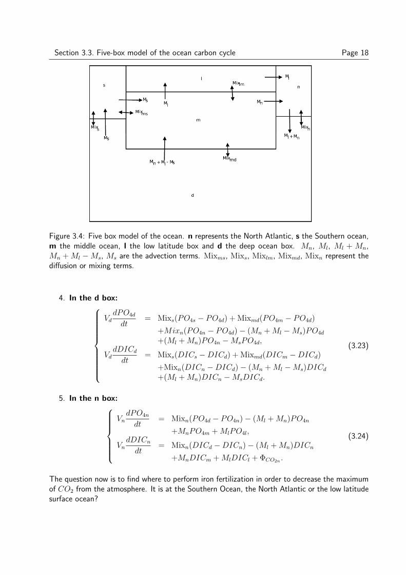
The boxes include (figure 3.4):

1. The s box for the Southern Ocean, where the water from the interior upwells carryingdissolved materials to the surface and creates the Antarctic Bottom Water (AABW) current.Part of this water from the interior advects in the middle ocean.


2. The l box for the low-latitude surface ocean. Here the water is warmer and the photo-synthesis process is more effective because of the presence of more light. Meanwhile, thepopulation of plankton in this area is not so high because of the lack of nutrients. It is alsothe area where the exchange rate between the atmosphere and the surface ocean is moreimportant. Gases such as carbon dioxide and oxygen are released back to the atmosphereeasily.

3. The n box for the North Atlantic. Here the water from the surface sinks to the deepocean, because of the difference in density (due to the temperature and salinity) , carryingdissolved materials from the surface to the deep.

4. The d box for the deep ocean. Here the dissolved organic matter can remain for a thousandyears [3] before being carried back to the surface by the overturning ocean circulation knownas the thermohaline circulation.

5. Finally the m box, for the middle ocean. This part of the ocean is called the thermocline(see figure 3.3). It is a transition layer between the mixed layer (or surface layer) atthe surface and the deep water layer, based on temperature. In the thermocline, thetemperature decreases rapidly from the mixed layer temperature to the much colder deepwater temperature. The mixed layer and the deep water layer are relatively uniform intemperature while the thermocline constitutes a transition between the two.

The circulation pattern of our model is as follows. Water from the deep upwells to the SouthernOcean. It is then advected to the middle ocean, from where it goes to the North Atlantic andsinks back to the deep ocean. Considering mass conservation, the equations for phosphate (PO4)and DIC are as follows:

1. In the s box:Vs

dPO4s

dt= Mixs(PO4d − PO4s) + Mixms(PO4m − PO4s)

+Ms(PO4d − PO4s),

VsdDICs

dt= Mixs(DICd −DICs) + Mixms(DICm −DICs)

+Ms(DICd −DICs) + ΦCO2s .

(3.20)

2. In the l box:Vl

dPO4l

dt= Mixlm(PO4m − PO4l) + Ml(PO4m − PO4l),

VldDICl

dt= Mixlm(DICm −DICl) + Ml(DICm −DICl)

+ΦCO2l.

(3.21)


Figure 3.3: A simple temperature - depth ocean water profile. We can see that temperaturedecreases with increasing depth. The thermocline is the layer of water where the temperaturechanges rapidly with depth. This temperature-depth profile is what we might expect to find inlow to middle latitudes.

3. In the m box:

VmdPO4m

dt= Mixms(PO4s − PO4m) + Mixlm(PO4l − PO4m)

+Mixmd(PO4d − PO4m) + (Mn + Ml −Ms)PO4d

+MsPO4s −MlPO4m −MnPO4m,

VmdDICm

dt= Mixms(DICs −DICm) + Mixlm(DICl −DICm)

+Mixmd(DICd −DICm) + (Mn + Ml −Ms)DICd

+MsDICs −MlDICm −MnDICm.

(3.22)


Figure 3.4: Five box model of the ocean. n represents the North Atlantic, s the Southern ocean,m the middle ocean, l the low latitude box and d the deep ocean box. Mn, Ml, Ml + Mn,Mn + Ml −Ms, Ms are the advection terms. Mixms, Mixs, Mixlm, Mixmd, Mixn represent thediffusion or mixing terms.

4. In the d box:

VddPO4d

dt= Mixs(PO4s − PO4d) + Mixmd(PO4m − PO4d)

+Mixn(PO4n − PO4d)− (Mn + Ml −Ms)PO4d

+(Ml + Mn)PO4n −MsPO4d,

VddDICd

dt= Mixs(DICs −DICd) + Mixmd(DICm −DICd)

+Mixn(DICn −DICd)− (Mn + Ml −Ms)DICd

+(Ml + Mn)DICn −MsDICd.

(3.23)

5. In the n box:Vn

dPO4n

dt= Mixn(PO4d − PO4n)− (Ml + Mn)PO4n

+MnPO4m + MlPO4l,

VndDICn

dt= Mixn(DICd −DICn)− (Ml + Mn)DICn

+MnDICm + MlDICl + ΦCO2n .

(3.24)

The question now is to find where to perform iron fertilization in order to decrease the maximumof CO2 from the atmosphere. It is at the Southern Ocean, the North Atlantic or the low latitudesurface ocean?


From the circulation pattern of our model, it appears that the warm water from the low latitudesas well as the middle ocean water are advected into the North Atlantic. In this area (the NorthAtlantic), the water which carries nutrients and DIC from the low latitude and middle ocean sinksinto the deep ocean. The result is the transportation of nutrients and DIC in the deep ocean.From this fact, the probability for the Particulate Organic Carbon (POC) from iron fertilizationin this region to sink in the deep ocean is high and could result in a net decrease of pCO2 in theatmosphere.

Another important region for iron fertilization could be the Southern Ocean. Here the upwellingof deep water with nutrients and DIC makes this area rich in nutrients. The nutrients can befixed into organic matter after photosynthesis. The organic matter will then sink or move, drivenby the thermocline in the middle ocean or perhaps in the North Atlantic, and return back intothe deep ocean. Since the overturning circulation of the ocean is relatively long (1000 years [3]),this could result in a transportation of DIC in the ocean interior.

For the low-latitude zone to be efficient, it is necessary that the advection term Ml be very high.Otherwise, all the POC produced by iron fertilization would be converted back into dissolvedorganic matter in the surface or sometimes the middle ocean and all the fixed carbon dioxide willreturn back to the atmosphere. This phenomenon is amplified by the fact that the water here iswarm and therefore less soluble for carbon dioxide.

Thus, the best area to experiment with iron fertilization seems to be the North Atlantic and theSouthern Ocean.

In the next section, using a code obtained with the use of the systems of equations 3.20, 3.21,3.22, 3.23, 3.24, we will simulate the iron fertilization experiment in the North Atlantic, the lowlatitudes and the Southern Ocean. We could therefore verify our hypothesis and give an answerto the question of where to do the experiment.

4. Simulation of iron fertilization with afive-box model

We are going to test the efficiency of iron fertilization in the ocean with the five-box model. Weconsider the ocean and the atmosphere together as a system in which the total concentration ofcarbon remains constant. This means that if the concentration of carbon dioxide decreases inthe atmosphere, it increases in the ocean and vice versa.

We will perform the simulation by forcing the concentration of nutrients at the ocean surfaceto decrease to zero. This is an exaggeration of what happens when enough iron is added atthe surface of the ocean[13]. Our experiments thus provide an upper limit to the effect ofadding enough iron to the ocean surface. The experiment will be performed in the SouthernOcean (experiment 1), the low-latitude surface ocean (experiment 2) and the North Atlantic(experiment 3). The analysis of the numerical output obtained will enable us to find an answerto our question: where should we perform iron fertilization to get atmospheric pCO2 to decreasemost?

4.1 Running the simulation

First of all, we set the values of the mixing and advection coefficients to be:

Mn = 10 Sv1, Ms = 10 Sv, Mixs = 0 Sv, Mixlm = 100 Sv, Mixn= 5 Sv, Mixms = 40 Sv, Mixmd

= 0 Sv, Ml = 0 Sv. This shows that the mixing terms between the Southern and the deep ocean,the middle and the deep ocean as well as the low latitude and the North Atlantic are neglected.The nutrients (phosphate) and DIC are initialized to their mean concentration values, which are:PO4 = 2.17 umol/kg and DIC = 2280 umol/kg. The partial pressure of carbon dioxide in theatmosphere is initialised to it pre-industrial value of 278 ppm [1]. We run the code in three steps:

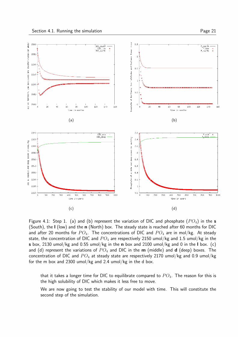
1. We initialised the concentration of phosphate and DIC to be the same and equal to theirmean values everywhere in the ocean. The goal of this step is to redistribute their values ineach box according to their different properties. After running the code for 1000 time stepsfor DIC and phosphate (PO4) in the deep and middle box, each time step representingone year and 160 time steps in the South, the North and the low latitudes box, each timestep representing 1 month, we plot the curve of DIC and PO4 with respect to time (figure4.1). At this stage, we fixed the partial pressure of carbon dioxide in the atmosphere to beconstant with time. The concentrations of PO4 and DIC obtained at steady state for eachbox are close to the real values measured in the ocean. These values increase from thesurface to the depth and constitute a good approximation to the actual ocean behaviour.The steady state is obtained faster for the surface ocean (North Atlantic, Southern Oceanand low latitude ocean) than for the middle and the deep ocean. This is due to the factthat the ocean interior is bigger and takes a longer time to adjust. Another observation is

11 Sv = 106m3/s

20

Section 4.1. Running the simulation Page 21

(a) (b)

(c) (d)

Figure 4.1: Step 1. (a) and (b) represent the variation of DIC and phosphate (PO4) in the s(South), the l (low) and the n (North) box. The steady state is reached after 60 months for DICand after 20 months for PO4. The concentrations of DIC and PO4 are in mol/kg. At steadystate, the concentration of DIC and PO4 are respectively 2150 umol/kg and 1.5 umol/kg in thes box, 2130 umol/kg and 0.55 umol/kg in the n box and 2100 umol/kg and 0 in the l box. (c)and (d) represent the variations of PO4 and DIC in the m (middle) and d (deep) boxes. Theconcentration of DIC and PO4 at steady state are respectively 2170 umol/kg and 0.9 umol/kgfor the m box and 2300 umol/kg and 2.4 umol/kg in the d box.

that it takes a longer time for DIC to equilibrate compared to PO4. The reason for this isthe high solubility of DIC which makes it less free to move.

We are now going to test the stability of our model with time. This will constitute thesecond step of the simulation.

Section 4.1. Running the simulation Page 22

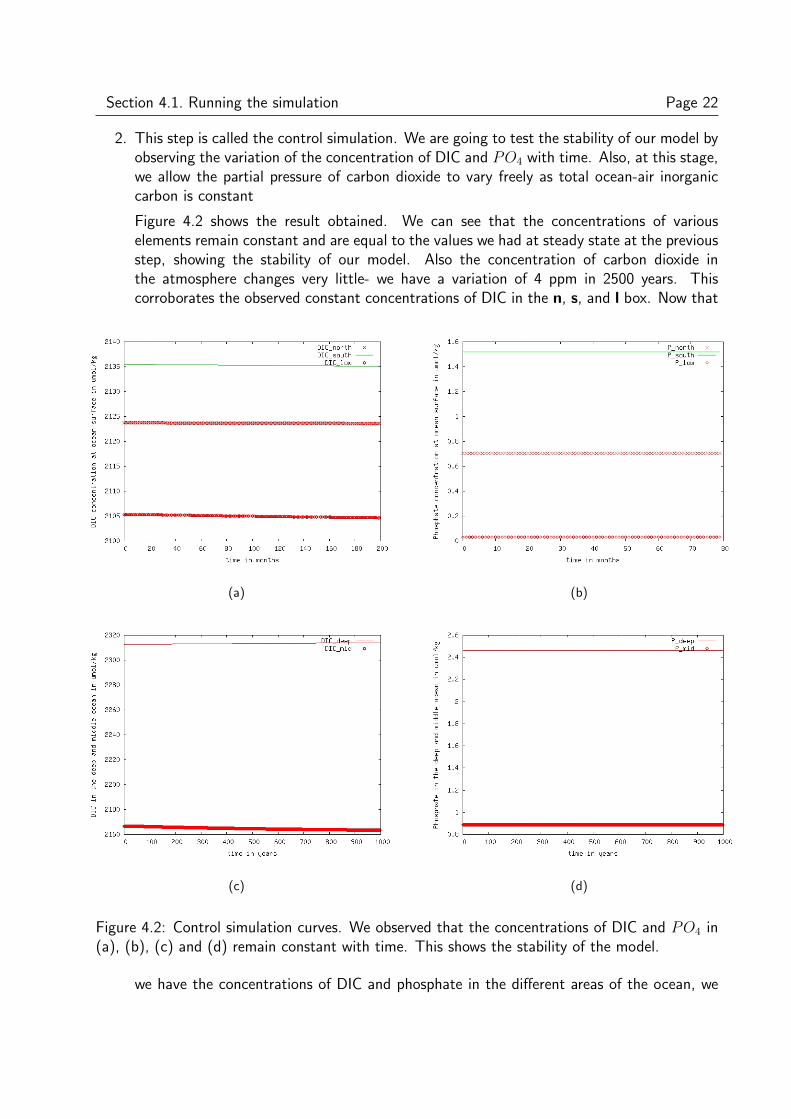
2. This step is called the control simulation. We are going to test the stability of our model byobserving the variation of the concentration of DIC and PO4 with time. Also, at this stage,we allow the partial pressure of carbon dioxide to vary freely as total ocean-air inorganiccarbon is constant

Figure 4.2 shows the result obtained. We can see that the concentrations of variouselements remain constant and are equal to the values we had at steady state at the previousstep, showing the stability of our model. Also the concentration of carbon dioxide inthe atmosphere changes very little- we have a variation of 4 ppm in 2500 years. Thiscorroborates the observed constant concentrations of DIC in the n, s, and l box. Now that

(a) (b)

(c) (d)

Figure 4.2: Control simulation curves. We observed that the concentrations of DIC and PO4 in(a), (b), (c) and (d) remain constant with time. This shows the stability of the model.

we have the concentrations of DIC and phosphate in the different areas of the ocean, we

Section 4.2. Discussion of the results Page 23

can start our fertilization experiment. This will constitute the final step.

3. The values of DIC and phosphate obtained at steady state during the previous step are usehere as initial values. We force nutrients (phosphate) to zero, by imposing a strong pro-ductivity of organic matter due to photosynthesis. This productivity is set by the followingequation:

production =PO4surface − P ∗

4t, (4.1)

where PO4surface is the concentration of phosphate at the surface in umol/kg and P ∗ isthe observed PO4 concentration. For the fertilization experiment, we set P ∗ = 0 in theregion of depletion, while setting P ∗ to its observed value in the rest of the ocean. Figures4.3 and 4.4 show the curves of DIC and phosphate (PO4) we obtained after simulatingthe fertilization in the North Atlantic, the low-latitudes surface ocean and the SouthernOcean. We can see that the effect of the productivity is to decrease gradually the nutrientconcentration in each fertilization area. The concentration of DIC and PO4 in the deepocean remains constant. This is due to the fact that the deep ocean represents more than80% of the total ocean volume. As a consequence, it acts like a reservoir. The supplyof nutrients from the surface due to fertilization is less significant compared to the totalquantity of nutrients in the deep ocean.

4.2 Discussion of the results

4.2.1 Fertilisation in the low latitude

Figure 4.5 shows a decrease in pCO2 from 278 ppm to 274 ppm after 2500 years of simulation,when the curve achieves steady state. This result shows that fertilization in the low latitudessurface ocean is not efficient. The reason for this is the poor concentration of nutrients. Fromchapter 2 we learnt that concentrations of phosphate and nitrate in this area are close to zero,due to the high mixing with the middle ocean, resulting in the transportation of nutrients into theocean interior ( the mixing term between the low and the middle ocean is 100 Sv and representsthe highest exchange rate). As a consequence, the population of phytoplankton is very low despitethe presence of enough light and iron brought by the dust from large deserts such as the Sahara.Our result suggests that an addition of iron will simply be a waste.

4.2.2 Fertilization in the North Atlantic

Figure 4.6 (a) shows the variation of atmospheric CO2 after depletion in the n box. We observea decrease of 35 ppm in the partial pressure of CO2 from 280 to 245 ppm at steady state. Itis difficult to have a better result because of the advection from the middle ocean (Mn = 10Sv) which brings back nutrients at the surface and thus decreases the overall productivity of thearea. Meanwhile, this result is much better than what we had for the low latitudes where nothingsignificant happens.


Figure 4.3: Variation of PO4 and DIC due to fertilization. We can observe the depletion ofnutrients in the n box. In the l box everything remains constant.

We have 267 ppm of atmospheric partial pressure after 150 years of fertilization, which is 6 ppmcloser to the 260 ppm observed after the last ice age [5]. This result is pretty good; but it is thebest? We are now going to test the fertilization in the Southern Ocean.


4.2.3 Fertilization in the Southern Ocean

The variation of the atmospheric CO2 in the s box is shown in figure 4.6 (b). The graph shows avariation of the partial pressure, from 278 ppm to 246 ppm at steady state. We can decomposethis in three parts: firstly, we have a strong drop from 278 ppm to 255 ppm, with a slope closeto the vertical, during the first hundred years. Then, the curve becomes smoother with a dropof the partial pressure from 255 ppm to 247 ppm after 1500 years. For the last part of the curvethe slope is close to the horizontal, meaning that it is approaching steady state. These successivechanges can be explained by the DIC behaviour in the Southern Ocean (see figure 4.4). Sincethe advection from the deep to the middle ocean is zero (Mn + Ml − Ms = 10 − 10 = 0),all the sinking water from the North Atlantic is advected in the Southern ocean, bringing moreDIC. Part of this moves to the middle ocean and another part equilibrates after a period of timewith the DIC taken up by the biological pump. Due to the difference in time frame, when theSouthern Ocean is fertilized, the DIC is removed quickly during the first year (see figure 4.4)and equilibrates later with that advected from the ocean interior, corresponding to the change ofslope for the atmospheric pCO2 (figure 4.6 (b)).

We observe a decrease of the partial pressure from 278 ppm to 250 ppm over 150 years, whichgives a drop of 28 ppm on figure 4.6 (b). This is more than the double what we had for theNorthern Atlantic simulation, and shows the strength of the fertilization in the Southern Ocean.

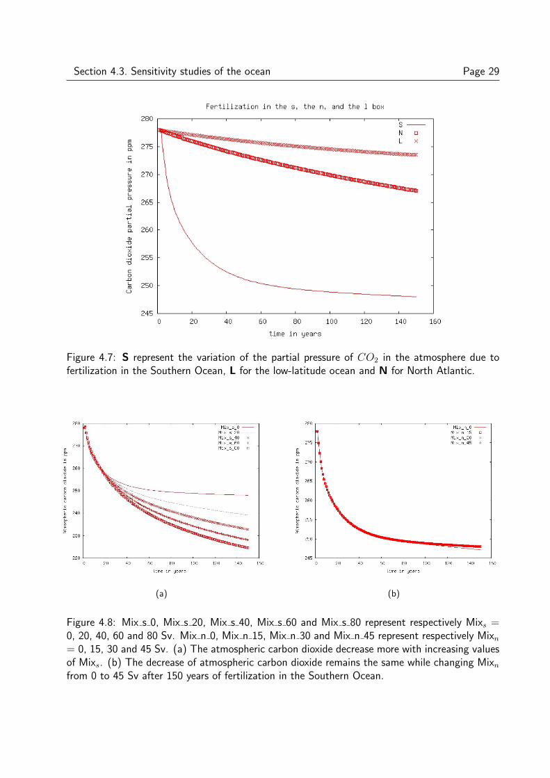
Figure 4.7 shows atmospheric pCO2 decreasing in all three fertilization scenarios for 150 years.The efficiency of the Southern Ocean in sequestering atmospheric pCO2 is more than twice thatof the North Atlantic.

It appears that the uptake of CO2 in the Southern Ocean is very efficient for the the first 500years of fertilization, as compared to the North Atlantic and the low latitudes. In particular,after 150 years of experiment, we have a drop of 28 ppm of atmospheric pCO2 for the SouthernOcean, only 11 ppm for the North Atlantic and almost nothing for the low latitudes. Meanwhile,after 2500 years of fertlization, when both curves have reached steady state, we observe thesame drop of atmospheric pCO2 for the North Atlantic and the Southern Ocean, but this timeframe is not interesting because it is very long. The reasons that the Southern Ocean and theNorth Atlantic are more efficient in the absorption of atmospheric CO2 is that they are areas ofdeep water formations and contain more unutilized nutrients compared to the low-latitude surfaceocean. The more the nutrients at the ocean surface, the stronger the biological production andthe taken up of CO2 from the atmosphere to the ocean.

Consequently, fertilization in the Southern Ocean presents the fastest solution in the uptake ofCO2 in the atmosphere and is therefore the most effective.

Trough out this study, we have consider the parameters of the ocean (mixings and advectionsterms) to be constants. What happens if those parameters change? It is clear today that, thechange of climate during the glacial-intergalacial period was not only a consequence of a strongproductivity of the ocean surface due to iron dust, but also a change in the mixings and advectionsterms between the high latitudes surface ocean and the deep ocean. We are now going to testthe behaviour of atmospheric carbon dioxide after a change in the ocean parameter. This is calledthe sensitivity studies.

Section 4.3. Sensitivity studies of the ocean Page 26

4.3 Sensitivity studies of the ocean

We perform Southern Ocean fertilization for a range of Mixs (0, 20 Sv, 40 Sv, 60 Sv, 80 Sv)and Mixn (0, 15 Sv, 30 Sv, 45 Sv) values. Figures 4.8 (a) and (b) show the output of thesimulation. It appears that increasing mixing between the Southern and deep ocean boxes resultsin a decrease of the atmospheric partial pressure of CO2, meaning that more carbon dioxide istaken up from the atmosphere by the ocean. Atmospheric pCO2 decreases by 33 ppm for Mixs

= 0, by 40 ppm for Mixs = 20 Sv and by 55 ppm for Mixs = 80 Sv.

After 150 years, changing mixing between the North Atlantic and the deep ocean (Mixn) has littleimpact on atmospheric pCO2. Meanwhile, a change may occur after a longer time frame. Thisdifference in the sequestration of carbon dioxide after changing Mixs and Mixn can be explainedby the size of the Southern Ocean which represents 0.22 % of the total surface ocean, and whichis very big compared to the 0.01% for the North Atlantic and by the larger quantities of nutrientsat the Southern Ocean surface compared to the North Atlantic. Therefore, the Southern Oceancontains and transports more nutrients and DIC than the North Atlantic. A change of in SouthernOcean parameters results in a more significant atmospheric CO2 drawdown.

The values of the parameters that we chosen for the fertilization simulation, Mixs = 0 andMixn = 5 Sv were guessed and are not probably the most suitables ones. However, our resultssuggest the critical importance of the Southern Ocean in the absorption of carbon dioxide fromthe atmosphere.


Figure 4.4: Variation of PO4 and DIC due to fertilization. We observe the depletion of nutrientsin the s box. In the m and the d box, the concentration of phosphate (Pmid, Pdeep) and DIC(DICmid, DICdeep) is almost constant after 200 years. For the fertilization in the s box, weobserve an increase of the concentration of DIC from 10 months onward. This is due to theupwelling of DIC from the deep (Ms = 10 Sv) which balances with the uptake of DIC due tofertilization.


(a) (b)

Figure 4.5: We can see that the variation of CO2 is the same in the control simulation (a) andin the fertilization of the low latitudes surface ocean (b).

(a) (b)

Figure 4.6: (a) We have a decrease of the partial pressure of 11 ppm after 150 years and 35 ppmafter 2500 years, which is very much greater than the 4 ppm drop during the control simulation(figure 4.5 (a)). (b) We observe a decrease of the partial pressure of 28 ppm after 150 years, and35 ppm after 2500 years.


Figure 4.7: S represent the variation of the partial pressure of CO2 in the atmosphere due tofertilization in the Southern Ocean, L for the low-latitude ocean and N for North Atlantic.

(a) (b)

Figure 4.8: Mix s 0, Mix s 20, Mix s 40, Mix s 60 and Mix s 80 represent respectively Mixs =0, 20, 40, 60 and 80 Sv. Mix n 0, Mix n 15, Mix n 30 and Mix n 45 represent respectively Mixn

= 0, 15, 30 and 45 Sv. (a) The atmospheric carbon dioxide decrease more with increasing valuesof Mixs. (b) The decrease of atmospheric carbon dioxide remains the same while changing Mixn

from 0 to 45 Sv after 150 years of fertilization in the Southern Ocean.

5. Conclusion

From our study it appears that the low-latitude surface ocean is not an area to be considered forthe fertilization experiments. This area, despite the presence of sunlight and enough iron broughtnaturally by large deserts, has the lowest abundance of nutrients and chlorophyll (see chapter 2.2).An addition of iron will simply be a waste. The Northern Atlantic is more interesting in that itis possible to sequester up to 11 ppm of atmospheric CO2 in 150 years. The Southern Oceanis the most suitable area with a decrease of CO2 partial pressure in the atmosphere of 28 ppmafter 150 years of continuous fertilization. Meanwhile, for a longer time frame, both the NorthAtlantic and the Southern Ocean give the same results (we have a drop of 35 ppm of atmosphericpCO2 after 2500 years). The reasons that the Southern Ocean and the North Atlantic are moreefficient is that they are areas of deep water formation and contain more unutilized nutrients,which could be used during fertilization to fix more pCO2 than at the low-latitude surface. TheSouthern Ocean is more efficient than the North Atlantic because it is bigger and has the highestsurface nutrients. For each experiment, we forced a strong biological productivity, dropping theconcentration of nutrients to zero in the area of fertilization. It is very difficult to achieve thatin reality but such simulations give an understanding of the ocean behaviour. The results weobtained are the outcome of the assumptions we made for the values of the mixing and theadvection parameters. A change of these values may result in a different response of the ocean.

Despite the uncertainty about the mixing parameters, the Southern Ocean has a key role inthe sequestration of carbon dioxide, because of its high surface nutrient concentration and itsimportant role in the formation of deep water.

It is now clear that if we consider seeding the ocean with iron as a quick solution to stop globalwarming, the Southern Ocean is the zone to consider, though we cannot predict, for a given period,the quantity of CO2 which will be removed from the atmosphere because of the simplicity ofour model. Another question then arises: for how long should we do the experiment? In otherwords, if we stop the fertilization would the partial pressure of CO2 in the atmosphere returnto its previous value? What would happen to all that iron and what would be the ecologicalconsequences? These are the questions we cannot give an answer to now, but shall consider forfurther studies.

30

Acknowledgements

I would like to take this opportunity to express my profound support and commitment to all thepeople who believe in the development of Africa through science.

I hereby express my special gratitude to the entire AIMS staff. I am very grateful to them forhaving given me the opportunity to study various aspects of science at a cutting-edge level.

Special thanks to Dr. Irina Marinov for providing me with material and enough of her time, andto Dr. Mark Tadross who accepted to guide me on this document.

Thanks also to my family and to all my relatives for their permanent support.

31

Bibliography

[1] I. Marinov and J. L. Sarmiento. The Ocean Carbon Cycle and Climate. Kluwer Academics,2004.

[2] J. H. Martin. Glacial-interglacial co2 change: the iron hypothesis. Paleoceanography, 5:1–13,1990.

[3] J. L. Sarmiento and J. R. Toggweiler. A new model for the role of the oceans in determiningatmospheric pco2. Nature, 308:1928–1950, 1984.

[4] J. L. Sarmiento and C. O. James. Three-dimensional simulations of the impact of southernocean nutrient depletion on atmospheric co2 and ocean chemistry. Limnology and Oceanog-raphy, 36:621–624, 1991.

[5] U. Siegenthaler and T. Wenk. Rapid atmospheric co2 variations and ocean circulation.Nature, 308:624–626, 1984.

[6] J. R. Toggweiler and M. K. Robert. Ocean circulation: Thermohaline circulation.http://cdiac.ornl.gov/oceans/GLODAP/glodap−pdfs/Thermohaline.web.pdf.

[7] J. L. Sarmiento and N. Gruber. Ocean biogeochemical dynamics. Princeton University press,2004.

[8] Noaa- nesdis- national oceanographic data center. http://www.nodc.noaa.gov/cgi-bin/OC5/WOA05F/woa05f.pl.

[9] Ocean color viewed from space. http://vathena.arc.nasa.gov/curric/oceans/ocolor/index.html.

[10] Espere climate encyclopedia. http://espere.mpch-mainz.mpg.de/documents/pdf/.

[11] P. Lam and S. W. Chisholm. Iron fertilization of oceans: Reconciling commercial claimswith published models. An unpublish paper, 2002.

[12] A. J. Watson. Volcanic iron, co2, ocean productivity and climate. Nature, 385:587–588,1997.

[13] P. W. Boyd, A. J. Watson, C. S. Law, E. R. Abraham, T. Trull, R. Murdoch, D. C. E.Bakker, A. R. Bowie, K. O. Buesseler, H. Chang, M. Charette, P. Croot, K. Downing,R. Frew, M. Gall, M. Hadfield, J. Hall, M. Harvey, G. Jameson, J. Laroche, M. Liddicoat,R. Ling, M. T. Maldonado, R. M. Mckay, S. Nodder, S. Pickmere, R. Primore, S. Rintoul,K. Safi, P. Sutton, R. Strzepek, K. Tanneberg, S. Turner, A. Waite, and J. Zeldis. A mes-ophytoplankton bloom in the polar southern ocean stimulated by iron fertilization. Nature,407:695–702, 2000.

[14] T. H. Peng and W. S. Broecker. Factor limiting the reduction of atmospheric co2 by ironfertilization. Limnology and Oceanography, 36:1919–1927, 1991.

32

BIBLIOGRAPHY Page 33

[15] Preliminary results of subarctic pacific iron experiment for ecosystem dynamics study (seeds)in 2001 and 2002. http://www.maff.go.jp/mud/476.html.

[16] P. W. Boyd, R. Strzepek, S. Takeda, G. Jackson, C. S. Wong, R. M. Mckay, C. Law,H. Kiyosawa, H. Saito, N. Sherry, K. Johnson, J. Gower, and N. Ramaiah. The evolution andtermination of an iron-induced mesoscale bloom in the northeast subarctic pacific. Limnologyand Oceanography, pages 1872–1886, 2005.

[17] Z. S. Kolber, R. T. Barber, K. H. Coale, S. E. Fitzwater, R. M. Greene, K. S. Johnson,S. Lindley, and P. G. Falkowski. Iron limitation of phytoplankton photosynthesis in theequatorial pacific ocean. Nature, 371:145–149, 1994.

iron fertilization in the ocean and consequences for the ... fertilization in the ocean and...

Documents