irreversibility, uncertainty, and...

Journal of Economic Literature Vol. XXIX (September 1991), pp. 1110-1148

Irreversibility, Uncertainty, and Investment

By ROBERT S. PINDYCK

Massachusetts Institute of Technology

My thanks to Prabhat Mehta for his research assistance, and to Ben Bernanke, Vittorio Corbo, Nalin Kulatilaka, Robert McDonald, Louis Serven, Andreas Solimano, and two anonymous referees for helpful comments and suggestions. Financial support was provided by MIT's Center for Energy Policy Research, by the World Bank, and by the National Science Foundation under Grant No. SES-8618502. Any errors are mine alone.

I. Introduction

DESPITE ITS IMPORTANCE to economic growth and market structure, the

investment behavior of firms, industries, and countries remains poorly understood. Econometric models have had limited success in explaining and predict- ing changes in investment spending, and we lack a clear explanation of why some countries or industries invest more than others.

One problem with existing models is that they ignore two important characteristics of most investment expenditures. First, the expenditures are largely irreversible; that is, they are mostly sunk costs that cannot be recovered. Second, the investments can be delayed, giving the firm an opportunity to wait for new information to arrive about prices, costs, and other market conditions before it commits resources.

As an emerging literature has shown, the ability to delay an irreversible invest-

ment expenditure can profoundly affect the decision to invest. It also undermines the theoretical foundation of standard neoclassical investment models, and in- validates the net present value rule as it is usually taught to students in business school: "Invest in a project when the present value of its expected cash flows is at least as large as its cost." This rule and models based on it-are incorrect when investments are irreversible and decisions to invest can be postponed.

Irreversibility may have important implications for our understanding of aggregate investment behavior. It makes investment especially sensitive to various forms of risk, such as uncertainty over the future product prices and operating costs that determine cash flows, uncertainty over future interest rates, and uncertainty over the cost and timing of the investment itself. Irreversibility may therefore have implications for macroeconomic policy; if a goal is to stimulate investment, stability and credibility

1110

This content downloaded from 18.7.29.240 on Wed, 5 Nov 2014 09:36:58 AMAll use subject to JSTOR Terms and Conditions

http://www.jstor.org/page/info/about/policies/terms.jsp

Pindyck: Irreversibility, Uncertainty, and Investment 1111

could be much more important than tax incentives or interest rates.

What makes an investment expenditure a sunk cost and thus irreversible? Usually it is the fact that the capital is firm or industry specific, that is, it cannot be used productively by a different firm or in a different industry. For example, most investments in marketing and ad- vertising are firm specific, and hence are clearly sunk costs. A steel plant is industry specific-it can only be used to produce steel. Although in principle the plant could be sold to another steel company, its cost should be viewed as mostly sunk, particularly if the industry is competitive. The reason is that the value of the plant will be about the same for all firms in the industry, so there is likely to be little gained from selling it. (If the price of steel falls so that a plant turns out, ex post, to have been a "bad" investment, it will also be viewed as a bad investment by other steel companies, so that the ability to sell the plant will not be worth much.)

Even investments that are not firm or industry specific are often partly irreversible because of the "lemons" problem. For example, office equipment, cars, trucks, and computers are not industry specific, but have resale value well below their purchase cost, even if new. Irreversibility can also arise because of government regulations or institutional arrangements. For example, capital controls may make it impossible for foreign (or domestic) investors to sell assets and reallocate their funds. And investments in new workers may be partly irreversible because of high costs of hiring, training, and firing.

Firms do not always have an opportunity to delay investments. For example, there can be occasions in which strategic considerations make it imperative for a firm to invest quickly and thereby preempt investment by existing or po-

tential competitors. (Richard Gilbert 1989 surveys the literature on strategic aspects of investment.) But in most cases, delay is at least feasible. There may be a cost to delay-the risk of entry by other firms, or simply foregone cash flows-but this cost must be weighed against the benefits of waiting for new information.

An irreversible investment opportunity is much like a financial call option. A call option gives the holder the right, for some specified amount of time, to pay an exercise price and in return receive an asset (e.g., a share of stock) that has some value. Exercising the option is irreversible; although the asset can be sold to another investor, one cannot retrieve the option or the money that was paid to exercise it. A firm with an investment opportunity likewise has the option to spend money (the "exercise price") now or in the future, in return for an asset (e.g., a project) of some value. Again, the asset can be sold to another firm, but the investment is irreversible. As with the financial call option, this option to invest is valuable in part because the future value of the asset obtained by investing is uncertain. If the asset rises in value, the net payoff from investing rises. If it falls in value, the firm need not invest, and will only lose what it spent to obtain the investment opportunity.

How do firms obtain investment opportunities? Sometimes they result from patents, or ownership of land or natural resources. More generally, they arise from a firm's managerial resources, tech- nological knowledge, reputation, market position, and possible scale, all of which may have been built up over time, and which enable the firm to productively undertake investments that individuals or other firms cannot undertake. Most important, these options to invest are valuable. Indeed, for most firms, a substantial part of their market value is attributable to their options to invest and grow in



1112 Journal of Economic Literature, Vol. XXIX (September 1991)

the future, as opposed to the capital they already have in place. (For discussions of growth options as sources of firm value, see Stewart Myers 1977; W. Carl Kester 1984; and my 1988 article.)

When a firm makes an irreversible investment expenditure, it exercises, or "kills," its option to invest. It gives up the possibility of waiting for new information to arrive that might affect the desir- ability or timing of the expenditure; it cannot disinvest should market conditions change adversely. This lost option value is an opportunity cost that must be included as part of the cost of the investment. As a result, the NPV rule "Invest when the value of a unit of capital is at least as large as its purchase and installation cost" must be modified. The value of the unit must exceed the purchase and installation cost, by an amount equal to the value of keeping the investment option alive.

Recent studies have shown that this opportunity cost of investing can be large, and investment rules that ignore it can be grossly in error.1 Also, this opportunity cost is highly sensitive to uncertainty over the future value of the project, so that changing economic conditions that affect the perceived riskiness of future cash flows can have a large impact on investment spending, larger than, say, a change in interest rates. This may help to explain why neoclassical investment theory has failed to provide good empirical models of investment behavior.

This paper has several objectives. First, I will review some basic models of irreversible investment to illustrate the option-like characteristics of investment opportunities, and to show how optimal investment rules can be obtained from methods of option pricing, or alternatively from dynamic programming. Be- sides demonstrating a methodology that can be used to solve a class of investment problems, this will show how the resulting investment rules depend on various parameters that come from the market environment.

A second objective is to survey briefly some recent applications of this methodology to a variety of investment problems, and to the analysis of firm and industry behavior. Examples will include the effects of sunk costs of entry, exit, and temporary shutdowns and restartups on investment and output decisions, the implications of construction time (and the option to abandon construction) for the value of a project, and the determinants of a firm's choice of capacity. I will also show how models of irreversible investment have helped to explain the preva- lence of "hysteresis," that is, the ten- dency for an effect (such as foreign sales in the U. S.) to persist well after the cause that brought it about (an appreciation of the dollar) has disappeared.

Finally, I will briefly discuss some of the implications that the irreversibility of investment may have for policy. For example, given the importance of risk, policies that stabilize prices or exchange rates may be particulary effective ways of stimulating investment. Similarly, a major cost of political and economic instability may be its depressing effect on investment.

Section II uses a simple two-period example to illustrate how irreversibility can affect an investment decision, and how option pricing methods can be used to value a firm's investment opportunity,

1 See, for example, Robert McDonald and Daniel Siegel (1986), Michael Brennan and Eduardo Schwartz (1985), Saman Majd and Pindyck (1987), and Pindyck (1988). Ben Bernanke (1983) and Alex Cukierman (1980) have developed related models in which firms have an incentive to postpone irreversible investments so that they can wait for new information to arrive. However, in their models, this information makes the future value of an investment less uncertain; we will focus on situations in which information arrives over time, but the future is always uncertain.




t=0 t= 1 t=2

P1 = $150 - P2= 150 -

q

P( = $100

(1--q P1 = $50 -- P2 = 50

Figure 1. Price of Widgets

and determine whether or not the firm should invest. Section III then works through a basic continuous-time model of irreversible investment that was first examined by McDonald and Siegel (1986). Here a firm must decide when to invest in a project whose value follows a random walk. I first solve this problem using option pricing methods and then by dynamic programming, and show how the two approaches are related. Section IV extends this model so that the price of the firm's output follows a random walk, and the firm can (temporarily) stop producing if price falls below variable cost. I show how both the value of the project and the value of the firm's option to invest in the project can be determined, and derive the optimal investment rule and examine its properties.

Sections III and IV require the use of stochastic calculus, but I explain the basic techniques and their application in the Appendix. However, readers who are less technically inclined can skip directly to Section V. That section surveys a number of extensions that have appeared in the literature, as well as other applications of the methodology, including the analysis of hysteresis. Section VI dis- cusses policy implications and suggests future research, and Section VII concludes.

II. A Simple Two-Period Example The implications of irreversibility and

the option-like nature of an investment

opportunity can be demonstrated most easily with a simple two-period example. Consider a firm's decision to invest irreversibly in a widget factory. The factory can be built instantly, at a cost I, and will produce one widget per year forever, with zero operating cost. Currently the price of widgets is $100, but next year the price will change. With probability q, it will rise to $150, and with probability (1 - q) it will fall to $50. The price will then remain at this new level forever. (See Figure 1.) We will assume that this risk is fully diversifiable, so that the firm can discount future cash flows using the risk-free rate, which we will take to be 10 percent.

For the time being we will set I = $800 and q = .5. (Later we will see how the investment decision depends on I and q.) Given these values for I and q, is this a good investment? Should we invest now, or wait a year and see whether the price goes up or down? Suppose we invest now. Calculating the net present value of this investment in the standard way, we get

00

NPV -800 + E 100/(1. 1)t t=O

- 800 + 1,100 = $300.

The NPV is positive; the current value of a widget factory is V0 = 1,100 > 800. Hence it would seem that we should go ahead with the investment.

This conclusion is incorrect, however, because the calculations above ignore a




cost-the opportunity cost of investing now, rather than waiting and keeping open the possibility of not investing should the price fall. To see this, calculate the NPV of this investment opportunity, assuming instead that we wait one year and then invest only if the price goes up:

NPV = (. 5)[ -800/1.1 + > 150/(1. 1)t] t=1

= 425/1.1 = $386.

(Note that in year 0, there is no expenditure and no revenue. In year 1, the $800 is spent only if the price rises to $150, which will happen with probability .5.) The NPV today is higher if we plan to wait a year, so clearly waiting is better than investing now.

Note that if our only choices were to invest today or never invest, we would invest today. In that case there is no option to wait a year, and hence no opportunity cost to killing such an option, so the standard NPV rule would apply. We would likewise invest today if next year we could disinvest and recover the $800 should the price fall. Two things are needed to introduce an opportunity cost into the NPV calculation-irreversibility, and the ability to invest in the future as an alternative to investing today. There are, of course, situations in which a firm cannot wait, or cannot wait very long, to invest. (One example is the anticipated entry of a competitor into a market that is only large enough for one firm. An- other example is a patent or mineral resource lease that is about to expire.) The less time there is to delay, and the greater the cost of delaying, the less will irreversibility affect the investment decision. We will explore this point again in Section III in the context of a more general model.

How much is it worth to have the flexibility to make the investment decision

next year, rather than having to invest either now or never? (We know that having this flexibility is of some value, because we would prefer to wait rather than invest now.) The value of this "flexibility option" is easy to calculate; it is just the difference between the two NPVs, that is, $386 - $300 = $86.

Finally, suppose there exists a futures market for widgets, with the futures price for delivery one year from now equal to the expected future spot price, $100.2 Would the ability to hedge on the futures market change our investment decision? Specifically, would it lead us to invest now, rather than waiting a year? The answer is no. To see this, note that if we were to invest now, we would hedge by selling short futures for five widgets; this would exactly offset any fluctuations in the NPV of our project next year. But this would also mean that the NPV of our project today is $300, exactly what it is without hedging. Hence there is no gain from hedging, and we are still better off waiting until next year to make our investment decision.

A. Analogy to Financial Options

Our investment opportunity is analogous to a call option on a common stock. It gives us the right (which we need not exercise) to make an investment expenditure (the exercise price of the option) and receive a project (a share of stock) the value of which fluctuates stochastically. In the case of our simple example, next year if the price rises to $150, we exercise

2 In this example, the futures price would equal the expected future price because we assumed that the risk is fully diversifiable. (If the price of widgets were positively correlated with the market portfolio, the futures price would be less than the expected future spot price.) Note that if widgets were storable and aggregate storage is positive, the marginal convenience yield from holding inventory would then be 10 percent. The reason is that because the futures price equals the current spot price, the net holding cost (the interest cost of 10 percent less the marginal convenience yield) must be zero.




our option by paying $800 and receive an asset that will be worth V1 = $1,650 (= 115O0/i.it). If the price falls to $50, this asset will be worth only $550, so we will not exercise the option. We found that the value of our investment opportunity (assuming that the actual decision to invest can indeed be made next year) is $386. It will be helpful to recalculate this value using standard option pricing methods, because later we will use such methods to analyze other investment problems.

To do this, let Fo denote the value today of the investment opportunity, that is, what we should be willing to pay today to have the option to invest in the widget factory, and let F1 denote its value next year. Note that F1 is a random variable; it depends on what happens to the price of widgets. If the price rises to $150, then F1 will equal S150/(1. 1)t - $800 = $850. If the price falls to $50, the option to invest will go unexercised, so that F1 will equal 0. Thus we know all possible values for F1. The problem is to find Fo, the value of the option today.

To solve this problem, we will create a portfolio that has two components: the investment opportunity itself, and a certain number of widgets. We will pick this number of widgets so that the portfolio is risk-free, that is, so that its value next year is independent of whether the price of widgets goes up or down. Because the portfolio will be risk-free, we know that the rate of return one can earn from holding it must be the risk-free rate. By setting the portfolio's return equal to that rate, we will be able to calculate the current value of the investment opportunity.

Specifically, consider a portfolio in which one holds the investment opportunity, and sells short n widgets. (If widgets were a traded commodity, such as oil, one could obtain a short position by bor- rowing from another producer, or by going short in the futures market. For the

moment, however, we need not be con- cerned with the actual implementation of this portfolio.) The value of this portfolio today is (Do = Fo - nP0 = Fo - 100n. The value next year, (I4 = F1 - nPI, depends on P1. If P1 = 150 so that F1 = 850, (DI = 850 -150n. If P1 = 50 so that F1 = 0, DI = -50n. Now, let us choose n so that the portfolio is risk- free, that is, so that (DI is independent of what happens to price. To do this, just set

850 - 150n =-50n,

or, n = 8.5. With n chosen this way, (DI = -425, whether the price goes up or down.

We now calculate the return from holding this portfolio. That return is the capital gain, (DI - (DO, minus any pay- ments that must be made to hold the short position. Because the expected rate of capital gain on a widget is zero (the expected price next year is $100, the same as this year's price), no rational investor would hold a long position unless he or she could expect to earn at least 10 percent. Hence selling widgets short will require a payment of . IPo = $10 per widget per year.3 Our portfolio has a short position of 8.5 widgets, so it will have to pay out a total of $85. The return from holding this portfolio over the year is thus (DI (Do - 85 = (- (Fo -

nP0) -85 = -425 - Fo + 850 -85 =

340 -Fo. Because this return is risk-free, we

know that it must equal the risk-free rate, which we have assumed is 10 percent, times the initial value of the portfolio, (Do= Fo - nP0:

340 - Fo= .1(Fo - 850).

'This is analogous to selling short a dividend-paying stock. The short position requires payment of the dividend, because no rational investor will hold the offsetting long position without receiving that dividend.




We can thus determine that Fo = $386. Note that this is the same value that we obtained before by calculating the NPV of the investment opportunity under the assumption that we follow the optimal strategy of waiting a year before deciding whether to invest.

We have found that the value of our investment opportunity, that is, the value of the option to invest in this project, is $386. The payoff from investing (exercising the option) today is $1,100 -

$800 = $300. But once we invest, our option is gone, so the $386 is an opportunity cost of investing. Hence the full cost of the investment is $800 + $386 = $1,186 > $1,100. As a result, we should wait and keep our option alive, rather than invest today. We have thus come to the same conclusion as we did by comparing NPVs. This time, however, we calculated the value of the option to invest, and explicitly took it into account as one of the costs of investing.

Our calculation of the value of the option to invest was based on the construction of a risk-free portfolio, which requires that one can trade (hold a long or short position in) widgets. Of course, we could just as well have constructed our portfolio using some other asset, or combination of assets, the price of which is perfectly correlated with the price of widgets. But what if one cannot trade widgets, and there are no other assets that "span" the risk in a widget's price? In this case one could still calculate the value of the option to invest the way we did at the outset-by computing the NPV for each investment strategy (invest today versus wait a year and invest if the price goes up), and picking the strategy that yields the highest NPV. That is essentially the dynamic programming approach. In this case it gives exactly the same answer, because all price risk is diversifiable. In Section III we will explore this connection between option pricing

and dynamic programming in more detail.

B. Changing the Parameters

So far we have fixed the direct cost of the investment, 1, at $800. We can obtain further insight by changing this number, as well as other parameters, and calculating the effects on the value of the investment opportunity and on the investment decision. For example, by going through the same steps as above, it is easy to see that the short position needed to obtain a risk-free portfolio depends on I as follows:

n = 16.5 - .011.

The current value of the option to invest is then given by

Fo = 750 - .4551.

The reader can check that as long as I > $642, Fo exceeds the net benefit from investing today (rather than waiting), which is V0 - I = $1,100 -1. Hence if I > $642, one should wait rather than invest today. However, if I = $642, Fo = $458 = V0 - 1, so that one would be indifferent between investing today and waiting until next year. (This can also be seen by comparing the NPV of investing today with the NPV of waiting until next year.) And if I < $642, one should invest today rather than wait. The reason is that in this case the lost revenue from waiting exceeds the opportunity cost of closing off the option of waiting and not investing should the price fall. This is illustrated in Figure 2, which shows the value of the option, Fo, and the net payoff, V0 - 1, both as functions of 1. For I > $642, Fo = 750 - .4551 > V0 - 1, so the option should be kept alive. How- ever, if I < $642, 750 - .4551 < V0 - 1, so the option should be exercised, and hence its value is just the net payoff, Vo - I.

We can also determine how the value




L,100 , a . l l l l l

L,000_ \

900 - Vo- I -

800 2 4

700 __\-

F00oI Fo r) F ~~~750-.4551 I

3000 -

200: -

100 _

0 200 400 600 562 800 1000

Figure 2. Option to Invest in Widget Factory

of the investment option depends on q, the probability that the price of widgets will rise next year. To do this, let us once again set I = $800. The reader can verify that the short position needed to obtain a risk-free portfolio is independent of q, that is, n= 8.5. The payment required for the short position, however, does depend on q, because the expected capital gain on a widget depends on q. The expected rate of capital gain is [E(P1) - PO]IPO = q - .5, so the required payment per widget in the short position is .1 -

(q - .5) = .6 - q. By following the same steps as above, it is easy to see that the value today of the option to invest is Fo = 773q. This can also be written as a function of the current value of the project, V0. We have V0 = 100 + 2(1OOq + 50)/(1. 1)t = 600 + lOOOq, so

Fo = .773Vo - 464. Finally, note that it is better to wait rather than invest today as long as Fo > V0 - I, or q < .88.

There is nothing special about the particular source of uncertainty that we in-

troduced in this problem. There will be a value to waiting (i.e., an opportunity cost to investing today rather than waiting for information to arrive) whenever the investment is irreversible and the net payoff from the investment evolves stochastically over time. Thus we could have constructed our example so that the uncertainty arises over future exchange rates, factor input costs, or government policy. For example, the payoff from investing, V, might rise or fall in the future depending on (unpredictable) changes in policy. Alternatively, the cost of the investment, I, might rise or fall, in response to changes in materials costs, or to a policy change, such as the granting or taking away of an investment subsidy or tax benefit.

In our example, we made the unrealis- tic assumption that there is no longer any uncertainty after the second period. In- stead, we could have allowed the price to change unpredictably each period. For example, we could posit that at t = 2,




if the price is $150, it could increase to $225 with probability q or fall to $75 with probability (1 - q), and if it is $50 it could rise to $75 or fall to $25. Price could rise or fall in a similar way at t = 3, 4, and so on. One could then work out the value of the option to invest, and the optimal rule for exercising that option. Although the algebra is messier, the method is essentially the same as for the simple two-period exercise we carried out above. (This is the basis for the bino- mial option pricing model. See John Cox, Stephen Ross, and Mark Rubinstein 1979 and Cox and Rubinstein 1985 for detailed discussions.) Rather than take this approach, in the next section we extend our example by allowing the payoff from the investment to fluctuate continuously over time.

The next two sections make use of continuous-time stochastic processes, as well as Ito's Lemma (which is essentially a rule for differentiating and integrating functions of such processes). These tools, which are becoming more and more widely used in economics and finance, provide a convenient way of analyzing investment timing and option valuation problems. I provide an introduction to the use of these tools in the Appendix for readers who are unfamiliar with them. Those readers might want to review the Appendix before proceeding. (Introduc- tory treatments can also be found in Rob- ert Merton 1971; Gregory Chow 1979; John Hull 1989; and A. G. Malliaris and William Brock 1982.) Readers who would prefer to avoid this technical material al- together can skip directly to Section V, although they will miss some insights by doing so.

III. A More General Problem of Investment Timing

One of the more basic models of irreversible investment is that of McDonald

and Siegel (1986). They considered the following problem: At what point is it optimal to pay a sunk cost I in return for a project whose value is V, given that V evolves according to a geometric Brownian motion:

dV = otVdt + aVdz (1)

where dz is the increment of a Wiener process, that is, dz = E(t)(dt)"2, with E(t) a serially uncorrelated and normally distributed random variable. Equation (1) implies that the current value of the project is known, but future values are log- normally distributed with a variance that grows linearly with the time horizon. (See the Appendix for an explanation of the Wiener process.) Thus although information arrives over time (the firm ob- serves V changing), the future value of the project is always uncertain.

McDonald and Siegel pointed out that the investment opportunity is equivalent to a perpetual call option, and deciding when to invest is equivalent to deciding when to exercise such an option. Thus, the investment decision can be viewed as a problem of option valuation (as we saw in the simple example presented in the previous section). I will rederive the solution to their problem in two ways, first using option pricing (contingent claims) methods, and then via dynamic programming. This will allow us to compare these two approaches and the assumptions that each requires. We will then examine the characteristics of the solution.

A. The Use of Option Pricing

As we have seen, the firm's option to invest, that is, to pay a sunk cost I and receive a project worth V, is analogous to a call option on a stock. Unlike most financial call options, it is perpetual-it has no expiration date. We can value this option and determine the optimal exercise (investment) rule using the




same methods used to value financial options. (For an overview of option pricing methods' and their application, see Cox and Rubinstein 1985; Hull 1989; and Scott Mason and Merton 1985.)

This approach requires one important assumption, namely that stochastic changes in V are spanned by existing assets. Specifically, it must be possible to find an asset or construct a dynamic portfolio of assets (i.e., a portfolio whose holdings are adjusted continuously as asset prices change), the price of which is perfectly correlated with V. This is equivalent to saying that markets are suffi- ciently complete that the firm's decisions do not affect the opportunity set available to investors. The assumption of spanning should hold for most commodities, which are typically traded on both spot and futures markets, and for manufactured goods to the extent that prices are correlated with the values of shares or portfo- lios. However, there may be cases in which this assumption will not hold; an example might be a new product unre- lated to any existing ones.

With the spanning assumption, we can determine the investment rule that maximizes the firm's market value without making any assumptions about risk preferences or discount rates, and the investment problem reduces to one of contingent claim valuation. (We will see shortly that if spanning does not hold, dynamic programming can still be used to maximize the present value of the firm's expected flow of profits, subject to an arbitrary discount rate.)

Let x be the price of an asset or dynamic portfolio of assets perfectly correlated with V, and denote by Pvm the correlation of V with the market portfolio. Then x evolves according to

dx = [Lxdt + uxdz,

and by the capital asset pricing model (CAPM), its expected return is pt =

r + 4)pvmO,c where r is the risk-free rate and 4) is the market price of risk. We will assume that a-, the expected percentage rate of change of V, is less than its risk-adjusted return Vt. (As will become clear, the firm would never invest if this were not the case. No matter what the current level of V, the firm would always be better off waiting and simply holding on to the option to invest.) We denote by 8 the difference between It and cx, that is, 8 = - at.

A few words about the meaning of 8 are in order, given the important role it plays in this model. The analogy with a financial call option is helpful here. If V were the price of a share of common stock, 8 would be the dividend rate on the stock. The total expected return on the stock would be pt = 8 + a-, that is, the dividend rate plus the expected rate of capital gain.

If the dividend rate 8 were zero, a call option on the stock would always be held to maturity, and never exercised prema- turely. The reason is that the entire return on the stock is captured in its price movements, and hence by the call option, so there is no cost to keeping the option alive. But if the dividend rate is positive, there is an opportunity cost to keeping the option alive rather than exercising it. That opportunity cost is the dividend stream that one forgoes by holding the option rather than the stock. Because 8 is a proportional dividend rate, the higher the price of the stock, the greater the flow of dividends. At some high enough price, the opportunity cost of forgone dividends becomes high enough to make it worthwhile to exercise the option.

For our investment problem, pt is the expected rate of return from owning the completed project. It is the equilibrium rate established by the capital market, and includes an appropriate risk premium. If 8 > 0, the expected rate of




capital gain on the project is less than Vt. Hence 8 is an opportunity cost of delaying construction of the project, and instead keeping the option to invest alive. If 8 were zero, there would be no opportunity cost to keeping the option alive, and one would never invest, no matter how high the NPV of the project. That is why we assume 8 > 0. On the other hand, if 8 is very large, the value of the option will be very small, because the opportunity cost of waiting is large. As 8 -) oc, the value of the option goes to zero; in effect, the only choices are to invest now or never, and the standard NPV rule will again apply.

The parameter 8 can be interpreted in different ways. For example, it could reflect the process of entry and capacity expansion by competitors. Or it can simply reflect the cash flows from the project. If the project is infinitely lived, then equation (1) can represent the evolution of V during the operation of the project, and 5V is the rate of cash flow that the project yields. Because we assume 8 is constant, this is consistent with future cash flows being a constant proportion of the project's market value. 4

Equation (1) is, of course, is an abstrac- tion from most real projects. For example, if variable cost is positive and the project can be shut down temporarily when price falls below variable cost, V will not follow a log-normal process, even if the output price does. Nonetheless, equation (1) is a useful simplification that

will help to clarify the main effects of irreversibility and uncertainty. We will discuss more complicated (and hopefully more realistic) models later.

B. Solving the Investment Problem

Let us now turn to the valuation of our investment opportunity, and the optimal investment rule. Let F = F(V) be the value of the firm's option to invest. To find F(V) and the optimal investment rule, consider the return on the following portfolio: Hold the option, which is worth F(V), and go short dF/dV units of the project (or equivalently, of the asset or portfolio x). Using subscripts to denote derivatives, the value of this portfolio is P = F - FvV. Note that this portfolio is dynamic; as V changes, Fv may change, in which case the composition of the portfolio will be changed.

The short position in this portfolio will require a payment of 6VFv dollars per time period; otherwise no rational investor will enter into the long side of the transaction. (To see this, note that an investor holding a long position in the project will demand the risk-adjusted return ptV, which includes the capital gain plus the dividend stream 8V. Because the short position includes Fv units of the project, it will require paying out 8VFv.) Taking this into account, the total return from holding the portfolio over a short time interval dt is

dF - FVdV - 8VFvdt.

We will see shortly that this return is risk-free. Hence to avoid arbitrage possibilities it must equal r(F - FvV)dt:

dF - FVdV - 6VFvdt = r(F - FvV)dt. (2)

To obtain an expression for' dF, use Ito's Lemma:

dF = FVdV + (1/2)Fv(dV)2. (3)

4A constant payout rate, 8, and required return, ji, imply an infinite project life. Letting CF denote the cash flow from the project,

T T

VO= CFte-1tdt fAVOe(R-8)te-1tdt, 0 0

which implies T = oo. If the project has a finite life, equation (1) cannot represent the evolution of V during the operating period. However, it can represent its evolution prior to construction of the project, which is all that matters for the investment decision. See Majd and Pindyck (1987, pp. 11-13), for a detailed discussion of this point.




(Ito's Lemma is explained in the Appen- dix. Note that higher-order terms vanish.) NoW substitute (1) for dV, with ox replaced by > - 8, and (dV)2 = cr2V2dt into equation (3):

dF = ( - )VFvdt + crVFvdz + (1/2)cu2V2Fvdt. (4)

Finally, substitute (4) into (2), rearrange terms, and note that all terms in dz can- cel out, so the portfolio is indeed risk- free:

(1/2)U2 V2Fw + (r - 5)VFV -rFO= . (5)

Equation (5) is a differential equation that F(V) must satisfy. In addition, F(V) must satisfy the following boundary conditions:

F(O) = 0. (6a)

F(V*) = V* - I. (6b)

FV(V*) = 1. (6c)

Condition (6a) says that if V goes to zero, it will stay at zero-an implication of the process (1)-so the option to invest will be of no value. V* is the price at which it is optimal to invest, and (6b) just says that upon investing, the firm receives a net payoff V* - I. Condition (6c) is called the "smooth pasting" condition. If F(V) were not continuous and smooth at the critical exercise point V*, one could do better by exercising at a different point.5

To find F(V), we must solve equation (5) subject to the boundary conditions (6a-6c). In this case we can guess a func- tional form, and determine by substitu- tion if it works. It is easy to see the solution to equation (5) that also satisfies condition (6a) is

(7) F(V) = aV3

where a is a constant, and ,3 is given by6

= 1/2 - (r - )/cr2 + {[r - 6)/U2 - 1/2]2 + 2r/cu2}1/2. (8)

The remaining boundary conditions, (6b) and (6c), can be used to solve for the two remaining unknowns: the constant a, and the critical value V* at which it is optimal to invest. By substituting (7) into (6b) and (6c), it is easy to see that

V*= PI/(P- 1) (9)

and a = (V* - I)/(V*)3. (10)

Equations (7-10) give the value of the investment opportunity, and the optimal investment rule, that is, the critical value V* at which it is optimal (in the sense of maximizing the firm's market value) to invest. We will examine the character- istic of this solution below. Here we simply point out that we obtained this solution by showing that a hedged (risk-free) portfolio could be constructed consisting of the option to invest and a short position in the project. However, F(V) must be the solution to equation (5) even if the option to invest (or the project) does not exist and could not be included in the hedge portfolio. All that is required is spanning, that is, that one could find or construct an asset or dynamic portfolio of assets (x) that replicates the stochastic dynamics of V. As Merton (1977) has shown, one can replicate the value function with a portfolio consisting only of the asset x and risk-free bonds, and be-

5Avinash Dixit (1988) provides a heuristic deriva- tion of this condition.

'The general solution to equation (5) is

F(V) = a1VP' + a2V02,

where I31 = 1/2 - (r- 2

+ {[(r - 8) - 1/2]2 + 2rl(/2}"12 > 1,

and P2= 1/2- (r- 8)/u2 - {[(r - 8)(J2- 1/2]2 + 2rl/o2}'12 < 0.

Boundary condition (6a) implies that a2 = 0, so the solution can be written as in equation (7).




cause the value of this portfolio will have the same dynamics as F(V), the solution to (5), F(V) must be the value function to avoid dominance.

As discussed earlier, spanning will not always hold. If that is the case, one can still solve the investment problem using dynamic programming. This is shown below.

C. Dynamic Programming

To solve the problem by dynamic programming, note that we want a rule that maximizes the value of our investment opportunity, F(V):

F(V) = max EJ[(VT- I)e 1T] (11)

where Et denotes the expectation at time t, T is the (unknown) future time that the investment is made, ,u is the discount rate, and the maximization is subject to equation (1) for V. We will assume that ,u > a-, and as before denote 8 = ,u- (x.

Because the investment opportunity, F(V), yields no cash flows up to the time T that the investment is undertaken, the only return from holding it is its capital appreciation. As shown in the Appendix, the Bellman equation for this problem is therefore

uF = (1/dt)E,dF. (12)

Equation (12) just says that the total in- stantaneous return on the investment opportunity, ,uF, is equal to its expected rate of capital appreciation.

We used Ito's Lemma to obtain equation (3) for dF. Now substitute (1) for dV and (dV)2 into equation (3) to obtain the following expression for dF:

dF = cxVFvdt + zrVFvdz + (1/2)o2V2Fwvdt.

Because Et(dz) = 0, (lldt)EtdF = oaVFv + (1/2)u 2V2FW, and equation (12) can be rewritten as:

(1/2)cu2V2Fw + acVFv - = 0

or, substituting ac = - 8,

(1/2)cu2V2Fv + (Vt- 8)VFV - VF= 0. (13)

Observe that this equation is almost identical to equation (5); the only difference is that the discount rate ,u replaces the risk-free rate r. The boundary conditions (6a-6c) also apply here, and for the same reasons as before. (Note that (6c) follows from the fact that V* is chosen to maximize the net payoff V* - I.) Hence the contingent claims solution to our investment problem is equivalent to a dynamic programming solution, under the assumption of risk neutrality.7

Thus if spanning does not hold, we can still obtain a solution to the investment problem, subject to some discount rate. The solution will clearly be of the same form, and the effects of changes in u- or 8 will likewise be the same. One point is worth noting, however. Without spanning, there is no theory for determining the "correct" value for the discount rate ,u (unless we make restrictive assumptions about investors' or managers' utility functions). The CAPM, for example, would not hold, so it could not be used to calculate a risk-adjusted discount rate.

D. Characteristics of the Solution

Assuming that spanning holds, let us examine the optimal investment rule given by equations (7-10). A few numeri-

'This result was first demonstrated by Cox and Ross (1976). Also, note that equation (5) is the Bell- man equation for the maximization of the net payoff to the hedge portfolio that we constructed. Because the portfolio is risk-free, the Bellman equation for that problem is

rP = -- VFv + (jIdt)EtdP. (i)

That is, the return on the portfolio, rP, equals the per period cash flow that it pays out (which is negative, because iVFV must be paid in to maintain the short position), plus the expected rate of capital gain. By substituting P = F - FvV and expanding dF as before, one can see that (5) follows from (i).




2.0 ' I '

1.8

1.6 -

1.4-

1.2-

5~1.0 I 4.1 0 =.3

0.8-

O I I _ 1/ 1 l I I I ~ ~ ~~~~~~~~~~I I

0.6 0.2

0.4- =0

0.2-

0 0.00 0.40 0.80 1.20 1.60 2.00 2.40 2.80

v

Figure 3. F(V) for a = 0.2, 0.3

Note: 8 = 0.04, r = 0.04,1 = 1

cal solutions will help to illustrate the results and show how they depend on the values of the various parameters. As we will see, these results are qualitatively the same as those that come out of standard option pricing models. Unless otherwise noted, in what follows we set r = .04, 8 = .04, and the cost of the investment, I, equal to 1.

Figure 3 shows the value of the investment opportunity, F(V), for r = .2 and .3. (These values are conservative for many projects; in volatile markets, the standard deviation of annual changes in a project's value can easily exceed 20 or 30 percent.) The tangency point of F(V) with the line V - I gives the critical value of V, V*; the firm should invest only if V ? V*. For any positive or, V* > L. Thus the standard NPV rule, "Invest when the value of a project is at least as great as its cost," must be modified to

include the opportunity cost of investing now rather than waiting. That opportunity cost is exactly F(V). When V < V*, V < I + F(V), that is, the value of the project is less than its full cost, the direct cost I plus the opportunity cost of "killing" the investment option.

Note that F(V) increases when of increases, and so too does the critical value V*. Thus uncertainty increases the value of a firm's investment opportunities, but decreases the amount of actual investing that the firm will do. As a result, when a firm's market or economic environment becomes more uncertain, the stock market value of the firm can go up, even though the firm does less investing and perhaps produces less! This should make it easier to understand the behavior of oil companies during the mid-1980s. During this period oil prices fell, but the perceived uncertainty over future oil




2.0 ,I , l

1.8 -

1.6-

1.4 -

1.2 -

> 1.0 _

0.8 -

0.6 - 6=.04

0.4 -6= 08

0.2 -

0 0.00 0.40 0.80 1.20 1.60 2.00 2.40 2.80

V

Figure 4. F(V) for 8 = 0.04, 0.08

Note: a = 0.2, r= 0.04, 1 = 1

prices rose. In response, oil companies paid more than ever for offshore leases and other oil-bearing lands, even though their development expenditures fell and they produced less.

Finally, note that our results regarding the effects of uncertainty involve no assumptions about risk preferences, or about the extent to which the riskiness of V is correlated with the market. Firms can be risk-neutral, and stochastic changes in V can be completely diversifiable; an increase in cr will still increase V* and hence tend to depress investment.

Figures 4 and 5 show how F(V) and V* depend on 8. Observe that an increase in 8 from .04 to .08 results in a decrease in F(V), and hence a decrease in the critical value V*. (In the limit as 8 -* co, F(V) ->O for V < I, and V* -, as Figure 5 shows.) The reason is that

as 8 becomes larger, the expected rate of growth of V falls, and hence the expected appreciation in the value of the option to invest and acquire V falls. In effect, it becomes costlier to wait rather than invest now. To see this, consider an investment in an apartment building, where 5V is the net flow of rental income. The total return on the building, which must equal the risk-adjusted market rate, has two components-this income flow plus the expected rate of capital gain. Hence the greater the income flow rela- tive to the total return on the building, the more one forgoes by holding an option to invest in the building, rather than owning the building itself.

If the risk-free rate, r, is increased, F(V) increases, and so does V*. The reason is that the present value of an investment expenditure I made at a future time T is Ie- rT, but the present value of




7 I I I ,

6

5

4

3

2

1~~~~~~~~~~~

o L I I X I 0.00 0.04 0.08 0.12 0.16 0.20 0.24 0.28 0.32

6

Figure 5. V* as a Function of 8

Note: a = 0.2, r = 0.04, I = 1

the project that one receives in return for that expenditure is Ve 8T. Hence with a fixed, an increase in r reduces the present value of the cost of the investment but does not reduce its payoff. But note that while an increase in r raises the value of a firm's investment options, it also results in fewer of those options being exercised. Hence higher (real) interest rates reduce investment, but for a different reason than in the standard model.

IV. The Value of a Project and the Decision to Invest

As mentioned earlier, equation (1) ab- stracts from most real projects. A more realistic model would treat the price of the project's output as a geometric random walk (and possibly one or more factor input costs as well), rather than making the value of the project a random

walk. It would also allow for the project to be shut down (permanently or temporarily) if price falls below variable cost. The model developed in the previous section can easily be extended in this way. In so doing, we will see that option pricing methods can be used to find the value of the project, as well as the optimal investment rule.

Suppose the output price, P. follows the stochastic process:

dP = c.Pdt + rPdz. (14)

We will assume that (x < ,u, where ,u is the market risk-adjusted expected rate of return on P or an asset perfectly correlated with P. and let 8 = ,u- ( as before. If the output is a storable commodity (e.g., oil or copper), 8 will represent the net marginal convenience yield from storage, that is, the flow of benefits (less storage costs) that the marginal stored unit




provides. We assume for simplicity that 8 is constant. (For most commodities, marginal convenience yield in fact fluctuates as the total amount of storage fluctuates.)

We will also assume the following: (i) Marginal and average production cost is equal to a constant, c. (ii) The project can be costlessly shut down if P falls below c, and later restarted if P rises above c. (iii) The project produces one unit of output per period, is infinitely lived, and the (sunk) cost of investing in the project is L.

We now have two problems to solve. First, we must find the value of this project, V(P). To do this, we can make use of the fact that the project itself is a set of options.8 Specifically, once the project has been built, the firm has, for each future time t, an option to produce a unit of output, that is an option to pay c and receive P. Hence the project is equivalent to a large number (in this case, infinite, because the project is assumed to last indefinitely) of operating options, and can be valued accordingly.

Second, given the value of the project, we must value the firm's option to invest in it, and determine the optimal exercise (investment) rule. This will boil down to finding a critical P*, where the firm in- vests only if P - P. As shown below, the two steps to this problem can be solved sequentially by the same methods used in the previous section.9

A. Valuing the Project

If we assume that uncertainty over P is spanned by existing assets, we can

value the project (as well as the option to invest) using contingent claim methods. Otherwise, we can specify a discount rate and use dynamic programming. We will assume spanning and use the first approach.

As before, we construct a risk-free portfolio: long the project and short Vp units of the output. This portfolio has value V(P) - VpP, and yields the instanta- neous cash flow j(P - c)dt - 5VpPdt, where j = 1 if P c so that the firm is producing, and j = 0 otherwise. (Recall that 6VpPdt is the payment that must be made to maintain the short position.) The total return on the portfolio is thus dV - VpdP + j(P - c)dt - 6VpPdt. Be- cause this return is risk-free, set it equal to r(V - VpP)dt. Expanding dV using Ito's Lemma, substituting (14) for dP, and rearranging yields the following differential equation for V:

(1/2)&P2VPP + (r - 5)PVp - rV + j(P - c) = 0. (15)

This equation must be solved subject to the following boundary conditions:

V(0) = 0. (16a) V(c-) = V(c+). (16b)

VP(c-)= Vp(c+). (16c) lim V = PI - clr. (16d)

P -c o

Condition (16a) is an implication of equation (14); that is, if P is ever zero it will remain zero, so the project then has no value. Condition (16d) says that as P becomes very large, the probability that over any finite time period it will fall below cost and production will cease becomes very small. Hence the value of the project approaches the difference between two perpetuities: a flow of revenue (P) that is discounted at the risk-adjusted rate li but is expected to grow at rate (x, and a flow of cost (c), which is constant and hence is discounted at the risk-free

8This point and its implications are discussed in detail in McDonald and Siegel (1985).

9Note that the option to invest is an option to purchase a package of call options (because the project is just a set of options to pay c and receive P at each future time t). Hence we are valuing a compound option. For examples of the valuation of compound financial options, see Robert Geske (1979) and Peter Carr (1988). Our problem can be treated in a simpler manner.




400 I ' I '

350 -

300 -

250-

200 -=.4

150-

100

50- 0

0 0 2 4 6 8 10 12 14 16 18 20

p

Figure 6. V(P) for a = 0, 0.2, 0.4

Note: 8 = .04, r= .04, c= 10

rate r. Finally, conditions (16b) and (16c) say that the project's value is a continuous and smooth function of P.

The solution to equation (15) will have two parts, one for P < c, and one for P -c. The reader can check by substitu- tion that the following satisfies (15) as well as boundary conditions (16a) and (16d):

w A2Pr 2 + plb-Clr , P ' C

where:1?

31 = 1/2 - (r- )/u2 + {[(r-)/U2 - 1/2]2 + 2r/ 2}"/2

and

12 = 1/2 - (r - )u2

-{[(r- b)/U2 - 1/2]2 + 2r/u 2}/2.

The constants A1 and A2 can be found by applying boundary conditions (16b) and (16c):

Al- r - 132(r-

A1 =r P(13 8- ) c(l-2).

2 r-(r - P2)

The solution (17) for V(P) can be interpreted as follows: When P < c, the project is not producing. Then, A1PP' is the value of the firm's options to produce in the future, if and when P increases. When P - c, the project is producing. If, irrespective of changes in P. the firm

10 By substituting (17) for V(P) into (15), the reader can check that PI and 32 are the solutions to the following quadratic equation:

(1/2)g2pl(p3 -1) + (r - 8)PI - r = 0.

Because V(O) = 0, the positive solution (1I > 1) must apply when P < c, and the negative solution (12 <

0) must apply when P > c. Note that P is the same as 1 in equation (8).




400

350 -

300 -

250-

8= .02 200

150- / .04

100-

50 =~~~~~~~~~~~~~ .08

0 0 2 4 6 8 10 12 14 16 is 20

p

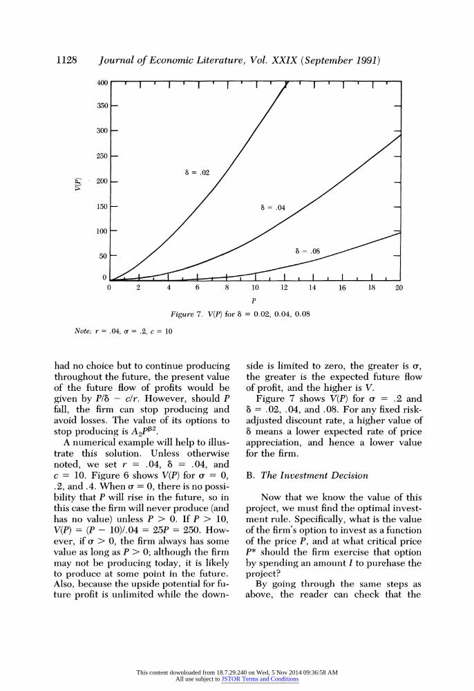
Figure 7. V(P) for 8 = 0.02, 0.04, 0.08

Note: r = .04, cr = .2, c = 10

had no choice but to continue producing throughout the future, the present value of the future flow of profits would be given by Plb - clr. However, should P fall, the firm can stop producing and avoid losses. The value of its options to stop producing is A2P2.

A numerical example will help to illustrate this solution. Unless otherwise noted, we set r = .04, 8 = .04, and c = 10. Figure 6 shows V(P) for cr = 0, .2, and .4. When r = 0, there is no possibility that P will rise in the future, so in this case the firm will never produce (and has no value) unless P > 0. If P > 10, V(P) = (P - 10)/.04 = 25P = 250. How- ever, if a > 0, the firm always has some value as long as P > 0; although the firm may not be producing today, it is likely to produce at some point in the future. Also, because the upside potential for future profit is unlimited while the down-

side is limited to zero, the greater is a, the greater is the expected future flow of profit, and the higher is V.

Figure 7 shows V(P) for a = .2 and 8 = .02, .04, and .08. For any fixed risk- adjusted discount rate, a higher value of 8 means a lower expected rate of price appreciation, and hence a lower value for the firm.

B. The Investment Decision

Now that we know the value of this project, we must find the optimal investment rule. Specifically, what is the value of the firm's option to invest as a function of the price P, and at what critical price P* should the firm exercise that option by spending an amount I to purchase the project?

By going through the same steps as above, the reader can check that the




500 . I I I I

400

300

200 > 22t}}10 0 ~~~~~F(P) </

0 0 t - 8 < 1lI 1 1 20 1 4V4 1 2 I 0

-100 0 4 8 12 16 20 24 28

P*= 23.8 p

Figure 8. V(P) -I and F(P) for a = 0.2, 8 = 0.04

Note: r = .04, c= 10, I = 100

value of the firm's option to invest, F(P), must satisfy the following differential equation:

(1/2)u2P2Fpp + (r - 8)PFp - rF = 0. (18)

F(P) must also satisfy the following boundary conditions:

F(0) = 0. (19a)

F(P*) = V(P*) - I. (19b)

Fp(P*) = Vp(P*). (19c)

These conditions can be interpreted in the same way as conditions (6a-6c) for the model presented in Section III. The difference is that the payoff from the investment, V, is now a function of the price P.

The solution to equation (18) and boundary condition (19a) is

F(P) = [aP 'I, P ' P* (20) V(P - I>,P>P*

where 1P is given above under equation (17). To find the constant a and the critical price P*, we use boundary conditions (19b) and (19c). By substituting equation (20) for F(P) and equation (17) for V(P) (for P - c) into (19b) and (19c), the reader can check that the constant a is given by

a = 2A2 (p*)(P2-PI) + j (P*)(l-P) (21)

and the critical price P* is the solution to

A2(PI - 12) (p*)P2

+ P* -I = 0. (22)

Equation (22), which is easily solved numerically, gives the optimal investment



700 ! I '

600

500

400

300

200

100

0

-100 l 10 20 t30

P:,0= 14.0 P __ 2 = 23.8 P*:,4 = 34.9

Figure 9. V(P) - I and F(P) for r = 0.0, 0.2, 0.4

Note: r = .04, 8 = .04, c = 10, I = 100

500 , I I , . I I

400 =.04

300

200

100

-10 0 4 8 12 16 20 24 28 f 32

p P 04 = 23.8 PL 08 = 29.2

Figure 10. V(P) - I and F(P) for 8 = 0.04, 0.08

Note: r = .04, r = .2, c = 10, I = 100




rule. (The reader can check first, that (22) has a unique positive solution for P* that is larger than c, and second, that V(P*) > I, so that the project must have an NPV that exceeds zero before it is optimal to invest.)

This solution is shown graphically in Figure 8, for a = .2, 8 = .04, and I = 100. The figure plots F(P) and V(P) - . Note from boundary condition (19b) that P* satisfies F(P*) = V(P*) - I, and note from boundary condition (19c) that P* is at a point of tangency of the two curves.

The comparative statics for changes in a or 8 are of interest. As we saw before, an increase in a results in an increase in V(P) for any P. (The project is a set of call options on future production, and the greater the volatility of price, the greater the value of these options.) But although an increase in ar raises the value of the project, it also increases the critical price at which it is optimal to invest, that is, aP*/&o. > 0. The reason is that for any P, the opportunity cost of investing, F(P), increases even more than V(P). Hence as with the simpler model presented in the previous section, increased uncertainty reduces investment. This is illustrated in Figure 9, which shows F(P) and V(P) - I for u = 0, .2, and .4. When u - 0, the critical price is 14, which just makes the value of the project equal to its cost of 100. As u is increased, both V(P) and F(P) increase; P* is 23.8 for u = .2 and 34.9 for u = .4.

An increase in 8 also increases the critical price P* at which the firm should invest. There are two opposing effects. If 8 is larger, so that the expected rate of increase of P is smaller, options on future production are worth less, so V(P) is smaller. At the same time, the opportunity cost of waiting to invest rises-the expected rate of growth of F(P) is smaller-so there is more incentive to exercise the investment option, rather than keep it alive. The first effect domi-

nates, so that a higher 8 results in a higher Pt. This is illustrated in Figure 10, which shows F(P) and V(P) - I for 8 = .04 and .08. Note that when 8 is increased, V(P) and hence F(P) fall sharply, and the tangency at P* moves to the right.

This result might at first seem to con- tradict what the simpler model of Section III tells us. Recall that in that model, an increase in 8 reduces the critical value of the project, V*, at which the firm should invest. But while in this model P* is higher when 8 is larger, the corresponding value of the project, V(P*), is lower. This can be seen from Figure 11, which shows P* as a function of a for 8 = .04 and .08, and Figure 12, which shows V(P*). If, say, cu is .2 and 8 is increased from 0.4 to .08, P* will rise from 23.8 to 29.2, but even at the higher P*, V is lower. Thus V* = V(P*) is declining with 8, just as in the simpler model.

This model shows how uncertainty over future prices affects both the value of a project and the decision to invest. As discussed in the next section, the model can easily be expanded to allow for fixed costs of temporarily stopping and restarting production, if such costs are important. Expanded in this way, models like this can have practical application, especially if the project is one that produces a traded commodity, like copper or oil. In that case, ou and 6 can be determined directly from futures and spot market data.

C. Alternative Stochastic Processes

The geometric random walk of equation (14) is convenient in that it permits an analytical solution, but one might be- lieve that the price, Pa is better repre- sented by a different stochastic process. For example, one could argue that over the long run, the price of a commodity will follow a mean-reverting process (for which the mean reflects long-run mar-




50

45

40

= .08

30-

25 - 8 =.04

20 -

15

10 _

5

0 I I 0 0.2 0.4

Ur

Figure 11. P* vs. a for 8 = 0.04, 0.08

1,000 ,

900

800

700

600

> 500

400 -

300 -

200 -

100,

0 0 0.2 0.4

Figure 12. V(P*) vs. or for 8 = 0.04, 0.08




ginal cost, and might be time-varying). Our model can be adapted to allow for this or foV alternative stochastic processes for P. However, in most cases numerical methods will then be necessary to obtain a solution.

As an example, suppose P follows the mean-reverting process:

dP/P = X(P - P)dt + adz. (23)

Here, P tends to revert back to a "normal" level P (which might be long-run marginal cost in the case of commodity like copper or coffee). By going through the same arguments as we did before, it is easy to show that V(P) must then satisfy the following differential equation:

(1/2)o2P2Vpp + [(r - ,- X)P + XP]PVp

-rV +j(P-c) = O (24)

together with boundary conditions (16a- 16c). The value of the investment option, F(P), must satisfy

(1/2)o2P2Fpp + [(r - - X)P + XP]PFp -rF= O (25)

with boundary conditions (19a-19c). Equations (24) and (25) are ordinary differential equations, so solution by numerical methods is relatively straightfor- ward.

V. Extensions

The models presented in the previous two sections are fairly simple, but illustrate how a project and an investment opportunity can be viewed as a set of options, and valued accordingly. These insights have been extended to a variety of problems involving investment and production decisions under uncertainty. This section reviews some of them.

A. Sunk Costs and Hysteresis

In Sections III and IV, we examined models in which the investment expendi-

ture is a sunk cost. Because the future value of the project is uncertain, this creates an opportunity cost to investing, which drives a wedge between the current value of the project and the direct cost of the investment.

In general, there may be a variety of sunk costs. For example, there may be a sunk cost of exiting an industry or aban- doning a project. This could include severance pay for workers, land reclama- tion in the case of a mine, and so on.11 This creates an opportunity cost of shutting down, because the value of the project might rise in the future. There may also be sunk costs associated with the operation of the project. In Section IV, we assumed that the firm could stop and restart production costlessly. For most projects, however, there are likely to be substantial sunk costs involved in even temporarily shutting down and restarting.

The valuation of projects and the decision to invest when there are sunk costs of this sort have been studied by Brennan and Schwartz (1985) and Dixit (1989a). Brennan and Schwartz (1985) find the effects of sunk costs on the decision to open and close (temporarily or permanently) a mine, when the price of the resource follows equation (14). Their model accounts for the fact that a mine is subject to cave-ins and flooding when not in use, and a temporary shutdown requires expenditures to avoid these possibilities. Likewise, reopening a temporarily closed mine requires a substantial expenditure. Finally, a mine can be permanently closed. This will involve costs of land rec- lamation (but avoids the cost of a temporary shutdown).

" Of course the scrap value of the project might exceed these costs. In this case, the owner of the project holds a put option (an option to "sell" the project for the net scrap value), and this raises the project's value. This has been analyzed by Myers and Majd (1985).




Brennan and Schwartz obtained an analytical solution for the case of an infinite resource stock. (Solutions can also be obtained when the resource stock is finite, but then numerical methods are required.) Their solution gives the value of the mine as a function of the resource price and the curent state of the mine (i.e., open or closed). It also gives the decision rule for changing the state of the mine (i.e., opening a closed mine or temporarily or permanently closing an open mine). Finally, given the value of the mine, Brennan and Schwartz show how (in principle) an option to invest in the mine can be valued and the optimal investment rule determined, using a contingent claim approach like that of Sec- tion IV. 12

By working through a realistic example of a copper mine, Brennan and Schwartz showed how the methods discussed in this paper can be applied in practice. But their work also shows how sunk costs of opening and closing a mine can explain the "hysteresis" often observed in extrac- tive resource industries: During periods of low prices, managers often continue to operate unprofitable mines that had been opened when prices were high; at other times managers fail to reopen seemingly profitable ones that had been closed when prices were low. This insight is further developed in Dixit (1989a, 1991), and is discussed below.

Dixit (1989a) studies a model with sunk costs k and 1, respectively, of entry and exit. The project produces one unit of output per period, with variable cost w. The output price, P, follows equation (14). If ar = 0, the standard result holds: Enter (i.e., spend k) if P - w + pk, and

exit if P ' w - pl, where p is the firm's discount rate. 13 However, if a > 0, there are opportunity costs to entering or exiting. These opportunity costs raise the critical price above which it is optimal to enter, and lower the critical price below which it is optimal to exit. (Further- more, numerical simulations show that r need not be large to induce a significant effect.)

These models help to explain the prev- alence of hysteresis-effects that persist after the causes that brought them about have disappeared. In Dixit's model, firms that entered an industry when price was high may remain there for an extended period of time even though price has fallen below variable cost, so they are losing money. (Price may rise in the future, and to exit and later reenter in- volves sunk costs.) And firms that leave an industry after a protracted period of low prices may hesitate to reenter, even after prices have risen enough to make entry seem profitable. Similarly, the Brennan and Schwartz model shows why many copper mines built during the 1970s when copper prices were high were kept open during the mid-1980s when copper prices had fallen to their lowest levels (in real terms) since the Great Depression.

The fact that exchange rate movements during the 1980s left the U. S. with a persistent trade deficit at the end of that decade can also be seen as a result of hysteresis. For example, Dixit (1989b) models entry by Japanese firms into the U. S. market when the exchange rate follows a geometric Brownian motion.

12 Jerey MacKie-Mason (1990) developed a related model of a mine that shows how nonlinear tax rules (such as a percentage depletion allowance) affect the value of the operating options as well as the investment decision.

13 As Dixit points out, one would find hysteresis if, for example, the price began at a level between w and w + pk, rose above w + pk so that entry occurred, but then fell to its original level, which is too high to induce exit. However, the firm's price expectations would then be irrational (because the price is in fact varying stochastically).




Again, there are sunk costs of entry and exit. The Japanese firms are ordered according to their variable costs, and all firms are price takers. As with the models discussed above, the sunk costs com- bined with exchange rate uncertainty create opportunity costs of entering or exiting the U.S. market. As a result, there will be an exchange rate band within which Japanese firms neither enter nor exit, and the U.S. market price will not vary as long as exchange rate fluctuations are within this band. Richard Baldwin (1988) and Baldwin and Paul Krugman (1989) developed related models that yield similar results. These models help to explain the low rate of exchange rate passthrough observed during the 1980s, and the persistence of the U. S. trade deficit even after the dollar depreciated. (Baldwin 1988 also provides empirical evidence that the over- valuation of the dollar during the early 1980s was indeed a hysteresis-inducing shock.)

Sunk costs of entry and exit can also have hysteretic effects on the exchange rate itself, and on prices. Baldwin and Krugman (1989), for example, show how the entry and exit decisions described above feed back to the exchange rate. In their model, a policy change (e.g., a reduction in the money supply) that causes the currency to appreciate sharply can lead to entry by foreign firms, which in turn leads to an equilibrium exchange rate that is below the original one. (These ideas are also discussed in Krugman 1989.) Similar effects occur with prices. In the case of copper, the reluctance of firms to close down mines during the mid-1980s, when demand was weak, allowed the price to fall even more than it would have otherwise.

Finally, sunk costs may be important in explaining the dependence of consumer spending, particularly for durable

goods, on income and wealth. Most pur- chases of consumer durables are at least partly irreversible. Poksang Lam (1989) developed a model that accounts for this, and shows how irreversibility results in a sluggish adjustment of the stock of durables to income changes. Sanford Gross- man and Guy Laroque (1990) study consumption and portfolio choice when consumption services are generated by a durable good and a transaction cost must be paid when the good is sold. Un- like in standard models (e.g., Merton 1971), optimal consumption is not a smooth funciton of wealth; a large change in wealth must occur before a consumer changes his holdings of durables and hence his consumption. As a result, the consumption-based CAPM fails to hold (although the market portfolio-based CAPM does hold).

B. Sequential Investment

Many investments occur in stages that must be carried out in sequence, and sometimes the payoffs from or costs of completing each stage are uncertain. For example, investing in a new line of aircraft begins with engineering, and continues with prototype production, testing, and final tooling stages. And an investment in a new drug by a pharmaceutical company begins with research that (with some probability) leads to a new compound, continues with extensive testing until FDA approval is obtained, and concludes with the construction of a production facility and marketing of the product.

Sequential investment programs like these can take substantial time to complete five to ten years for the two examples mentioned above. In addition, they can be temporarily or permanently aban- doned midstream if the value of the end product falls, or the expected cost of completing the investment rises. Hence




these investments can be viewed as compound options; each stage completed (or dollar invested) gives the firm an option to complete the next stage (or invest the next dollar). The problem is to find a contingent plan for making these sequential and irreversible expenditures

Majd and Pindyck (1987) solve this problem for a model in which a firm in- vests continuously (each dollar spent buys an option to spend the next dollar) until the project is completed, investment can be stopped and later restarted costlessly, and there is a maximum rate at which outlays and construction can proceed (i.e., it takes "time to build"). The payoff to the firm upon completion is V, the value of the operating project, which follows the geometric Brownian motion of equation (1). Letting K be the total remaining expenditure required to complete the project, the optimal rule is to keep investing at the maximum rate as long as V exceeds a critical value V*(K), with dV*/dK < 0. Using the methods of Sections III and IV, it is straight- forward to derive a partial differential equation for F(V, K), the value of the investment opportunity. Solutions to this equation and its associated boundry conditions, which are obtained by numerical methods, yield the optimal investment rule V*(K). 4

These solutions show how time to build magnifies the effects of irreversibility and

uncertainty. The lower the maximum rate of investment (i.e., the longer it takes to complete the project), the higher is the critical V*(K) required for construction to proceed. This is because the project's value upon completion is more uncertain, and the expected rate of growth of V over the construction period is less than p, the risk-adjusted rate of return (8 is positive). Also, unlike the model of Section III where the critical value V* declines monotonically with 8, with time to build, V* will increase with 8 when 8 is large. The reason is that while a higher 8 increases the opportunity cost of waiting to begin construction, it also reduces the expected rate of growth of V during the construction period, so that the (risk-adjusted) expected payoff from completing construction is reduced. Fi- nally, by computing F(V, K) for different maximum rates of investment, one can value construction time flexibility, that is, what one would pay to be able to build the project faster.'5

In the Majd-Pindyck model, investment occurs as a continuous flow; that is, each dollar spent gives the firm an option to spend another dollar, up to the last dollar, which gives the firm a completed project. Often, however, sequential investments occur in discrete stages, as with the aircraft and pharmaceutical examples mentioned above. In these cases, the optimal investment rules can be found by working backward from the

14 Letting k be the maximum rate of investment, this equation is

'/2u2V2Fvv + (r - 8)VFv - rF - x(kFK + k) = 0

where x = 1 when the firm is investing and 0 otherwise. F(V, K) must also satisfy the following boundary conditions:

F(V, 0) = V, limv ),O FV(V, K) = e bKlk

F(O, K) = 0 and F(V, K) and FV(V, K) continuous at the boundary V*(K). For an overview of numerical methods for solving partial differential equations of this kind, see Geske and Kuldeep Shastri (1985).

15 The production decisions of a firm facing a learning curve and stochastically shifting demand is another example of this kind of sequential investment. Here, part of the firm's cost of production is actually an (irreversible) investment, which yields a reduction in future costs. Because demand fluctuates, the future payoffs from this investment are uncertain. Majd and Pindyck (1989) introduce stochastic demand into a learning curve model, and derive the optimal production rule. They show how uncertainty Over future demand reduces the shadow value of cumulative production generated by learning, and thus raises the critical price at which it is optimal for the firm to produce.




completed project, as we did with the model of Section IV.

To see how this can be done, consider a two-stage investment in new oil production capacity. First, reserves of oil must be obtained, through exploration or outright purchase, at a cost 11. Second, development wells (and possibly pipe- lines) must be built, at a cost 12. Let P be the price of oil and assume it follows the geometric Brownian motion of equation (14). The firm thus begins with an option, worth F1(P), to invest in reserves. Doing so buys an option, worth F2(P), to invest in development wells. Making this investment yields production capacity, worth V(P).

Working backward to find the optimal investment rules, first note that as in the model of Section IV, V(P) is the value of the firm's operating options, and can be calculated accordingly. Next, F2(P) can be found; it is easy to show that it must satisfy equation (18) and boundary conditions (19a-19c), with 12 replacing I, and P* becoming the critical price at which the firm should invest in development wells. Finally, F1(P) can be found. It also satisfies (18) and (19a-19c), but with F2(P) replacing V(P) in (19b) and (19c), 1 replacing I, and P** replacing P*. (P** is the critical price of oil at which the firm should invest in reserves.) If marginal production cost is constant and there is no cost to stopping or restarting production, an analytical solution can be obtained. 16

In this example there is no time to build; each stage (obtaining reserves, and building development wells) can be completed instantly. For many projects each stage of the investment takes time, and the firm can stop investing in the middle

of a stage. Then the problem must be solved numerically, using a method like the one in Majd and Pindyck (1987).17

In all of the models discussed so far, no learning takes place, in the sense that future prices (or project values, V) are always uncertain, and the degree of uncertainty depends only on the time horizon. For some sequential investments, however, early stages provide information about costs or net payoffs in later stages. Synthetic fuels was a much de- bated example of this; oil companies ar- gued that demonstration plants were needed (and deserved funding by the government) to determine production costs. The aircraft and pharmaceutical investments mentioned above also have these characteristics. The engineering, prototype production, and testing stages in the development of a new aircraft all provide information about the ultimate cost of production (as well as the aircraft's flight characteristics, which will help determine its market value). Likewise, the R & D and testing stages of the development of a new drug determine the effi- cacy and side effects of the drug, and hence its value.

Kevin Roberts and Martin Weitzman (1981) developed a model of sequential investment that stresses this role of information gathering. In their model, each stage of investment yields information that reduces the uncertainty over the value of the completed project. Because the project can be stopped in midstream, it may pay to go ahead with the early stages of the investment even though ex ante the net present value of the entire project is negative. Hence the use of a simple net present value rule can reject

16 James Paddock, Siegel, and James Smith (1988) value oil reserves as options to produce oil, but ignore the development stage. Octavio Tourinho (1979) first suggested that natural resource reserves can be valued as options.

17 In a related paper, Carliss Baldwin (1982) ana- lyzes sequential investment decisions when investment opportunities arrive randomly, and the firm has limited resources to invest. She values the sequence of opportunities, and shows that a simple NPV rule will lead to overinvestment.




projects that should be undertaken. This is just the opposite of our earlier finding that a simple NPV rule can accept projects that should be rejected. The crucial assumption in the Roberts-Weitzman model is that prices and costs do not evolve stochastically. The value of the completed project may not be known (at least until the early stages are completed), but that value does not change over time, so there is no gain from waiting, and no opportunity cost to investing now. Instead, information gathering adds a shadow value to the early stages of the investment. 18

This result applies whenever information gathering, rather than waiting, yields information. The basic principle is easily seen by modifying our simple two-period example from Section II. Suppose that the widget factory can only be built this year, and at a cost of $1,200. However, by first spending $50 to research the widget market, one could determine whether widget prices will rise or fall next year. Clearly one should spend this $50, even though the NPV of the entire project (the research plus the construction of the factory) is negative. One would then build the factory only if the research showed that widget prices will rise.

C. Incremental Investment and Capacity Choice

So far we have examined decisions to invest in single, discrete projects, for example, the decision to build a new factory or develop a new aircraft. Much of

the economics literature on investment, however, focuses on incremental investment; firms invest to the point that the cost of the marginal unit of capital just equals the present value of the revenues it is expected to generate. The cost of the unit can include adjustment costs (re- flecting the time and expense of installing and learning to use new capital) in addition to the purchase cost. In most models, adjustment costs are a convex function of the rate of investment, and are thus a crucial determinant of that rate. (For an overview, see Stephen Nickell 1978 or the more recent survey by An- drew Abel 1990.)

Except for work by Kenneth Arrow (1968) and Nickell (1974), which is in a deterministic context, this literature generally ignores the effects of irreversibility. As with discrete projects, irreversibility and the ability to delay investment decisions change the fundamental rule for investing. The firm must include as part of the total cost of an incremental unit of capital the opportunity cost of investing in that unit now rather than waiting.

Giuseppe Bertola (1989) and Pindyck (1988) developed models of incremental investment and capacity choice that account for irreversibility. In Pindyck's model, the firm faces a linear inverse demand function, P = 0(t) - yQ, where 0 follows a geometric Brownian motion, and has a Leontief production technology. The firm can invest at any time at a cost k per unit of capital, and each unit of capital gives it the capacity to produce up to one unit of output per period. The investment problem is solved by first determining the value of an incremental unit of capital, given 0 and an existing capital stock, K, and then finding the value of the option to invest in this unit and the optimal exercise rule. This rule is a function K*(0)- invest whenever K < K*(o) which determines the firm's

'8 Weitzman (1981) used this model to evaluate the case for building demonstration plants for synthetic fuel production, and found that learning about costs could justify these early investments. Much of the debate over synthetic fuels has had to do with the role of government, and in particular whether subsidies (for demonstration plants or for actual production) could be justified. These issues are discussed in Paul Joskow and Pindyck (1979) and Richard Schmalensee (1980).




optimal capital stock. Pindyck shows that an increase in the variance of 0 increases the value of an incremental unit of capital (that unit represents a set of call options on future production), but increases the value of the option to invest in the unit even more, so that investment requires a higher value of 0. Hence a more volatile demand implies that a firm should hold less capital, but have a higher market value. 19

In Bertola's model, the firms' net revenue function is of the form AK'-Z, with O < 3 < 1. (This would follow from a Cobb-Douglas production function and an isoelastic demand curve.) The demand-shift variable Z and the purchase price of capital follow correlated geometric Brownian motions. Bertola solves for the optimal investment rule, and shows that the marginal profitability of capital that triggers investment is higher than the user cost of capital as conventionally measured. The capital stock, K, is nonsta- tionary, but Bertola finds the steady-state distribution for the ratio of the marginal profitability of capital to its price. Irre- versibility and uncertainty reduce the mean of this ratio; that is, on average capital intensity is higher. Although the firm has a higher threshold for investment, this is outweighed on average by low outcomes for Z.

The finding that uncertainty over future demand can increase the value of a marginal unit of capital is not new. All that is required is that the marginal revenue product of capital be convex in price. This is the case when the unit of capital can go unutilized (so that it represents a set of operating options). But as Richard

Hartman (1972) pointed out, it is also the case for a competitive firm that combines capital and labor with a linear homoge- neous production function. Hartman shows that as a result, price uncertainty increases the firm's investment and capital stock.

Andrew Abel (1983) extends Hartman's result to a dynamic model in which price follows a geometric Brownian motion and there are convex costs of adjusting the capital stock, and again shows that uncertainty increases the firm's rate of investment. Finally, Ricardo Caballero (1991) introduces asymmetric costs of adjustment to allow for irreversibility (it can be costlier to reduce K than to increase it), and shows that again price uncertainty increases the rate of investment. However, the Abel and Caballero results hinge on the assumptions of constant returns and perfect competition, which make the marginal revenue product of capital independent of the capital stock. Then the firm can ignore its future capital stock (and hence irreversibility) when deciding how much to invest today. As Ca- ballero shows, decreasing returns or im- perfect competition will link the marginal revenue products of capital across time, so that the basic result in Pindyck (1988) and Bertola (1989) holds.20

The assumption that the firm can invest incrementally is extreme. In most industries, capacity additions are lumpy, and there are scale economies (a 400 room hotel usually costs less to build and operate than two 200 room hotels).

19 This means that the ratio of a firm's market value to the value of its capital in place should always exceed one (because part of its market value is the value of its growth options), and this ratio should be higher for firms selling in more volatile markets. Kester's (1984) study suggests that this is indeed the case.

20 Even if firms are perfectly competitive and have constant returns, stochastic fluctuations in demand will depress irreversible investment if there can be entry by new firms in response to price increases. See Pindyck (1990b) for a discussion of this point. Also, Abel, Bertola, Caballero, and Pindyck examine the effects of increased demand or price uncertainty holding the discount rate fixed. As Roger Craine (1989) points out, an increase in demand uncertainty is likely to be accompanied by an increase in the systematic riskiness of the firm's capital, and hence an increase in its risk-adjusted discount rate.




Hence firms must decide when to add capacity, and how large an addition to make. This problem was first studied in a stochastic setting by Alan Manne (1961). He considered a firm that must always have enough capacity to satisfy demand, which grows according to a simple Brownian motion with drift. The cost of adding an amount of capacity x is kXa, with 0 < a < 1; the firm must choose x to minimize the present value of expected capital costs. Manne shows that with scale economies, uncertainty over demand growth leads the firm to add capacity in larger increments, and increases the present value of expected costs.

In Manne's model (which might apply to an electric utility that must always satisfy demand) the firm does not choose when to invest, only how much. Most firms must choose both. Pindyck (1988) determined the effects of uncertainty on these decisions when there are no scale economies in construction by extending his model to a firm that must decide when to build a single plant and how large it should be. 21 As with Manne's model, uncertainty increases the optimal plant size. However, it also raises the critical demand threshold at which the plant is built. Thus demand uncertainty should lead firms to delay capacity additions, but makes those additions larger when they occur.

Sometimes capacity choice is accompanied by a technology choice. Consider a firm that produces two products, A and B, with interdependent demands that

vary stochastically. It can produce these products by (irreversibly) installing and utilizing product-specific capital, or by (irreversibly) installing a more costly flexible type of capital that can be used to produce either or both products. The problem is to decide which type and how much capital to install. Hua He and Pin- dyck (1989) solve this for a model with linear demands by first valuing incremental units of capital (output-specific and flexible), and then finding the optimal investment rule, and hence optimal amounts of capacity. By integrating the value of incremental units of specific and flexible capital, one can determine the preferred type of capital, as well as the value (if any) of flexibility.

In all of the studies cited so far, the stochastic state variable (the value of the project, the price of the firm's output, or a demand- or cost-shift variable) is specified exogenously. In a competitive equilibrium, firms' investment and output decisions are dependent on the price process, but also collectively generate that process. Hence we would like to know whether firms' decisions are consistent with the price processes we specify.

At least two studies have addressed this issue. Steven Lippman and Richard P. Rumelt (1985) model a competitive industry where firms face sunk costs of entry and exit, and the market demand curve fluctuates stochastically. They find an equilibrium consisting of optimal investment and production rules for firms (with uncertainty, they hold less capacity), and a corresponding process for market price. John Leahy (1989) extends Dixit's (1989a) model of entry and exit to an industry setting in which price is endogenous. He shows that price will be driven by demand shocks until an entry or exit barrier is reached, and then entry or exit prevent it from moving further. Hence price follows a regulated Brownian motion. Surprisingly, it makes

21 The firm has an option, worth G(K, 0), to build a plant of arbitrary size K. Once built, the plant has a value V(K, 0) (the value of the firm's operating options), which can be found using the methods of Section IV. G(K, 0) will satisfy equation (18), but with boundary conditions G(K*, 0*) = V(K*, 0*) - kK* and GO(K*,0*) = VO(K*, 0*), where 0* is the critical 0 at which the plant should be built, and K* is its optimal size. See the Appendix to Pindyck (1988).




no difference whether firms take entry and exit into account, or simply assume that price will follow a geometric Brownian motion; the same entry and exit barriers result. This suggests that models in which price is exogenous may provide a reasonable description of industry investment and capacity.

VI. Investment Behavior and Economic Policy

Nondiversifiable risk plays a role in even the simplest models of investment, by affecting the cost of capital. But the findings summarized in this paper sug- gest that risk may be a more crucial determinant of investment. This is likely to have implications for the explanation and prediction of investment behavior at the industry- or economy-wide level, and for the design of policy.

The role of interest rates and interest rate stability in determining investment is a good example of this. Jonathan Inger- soll and Ross (1988) have examined irreversible investment decisions when the interest rate evolves stochastically, but future cash flows are known with certainty. As with uncertainty over future cash flows, this creates an opportunity cost of investing, so that the traditional NPV rule will accept too many projects. Instead, an investment should be made only when the interest rate is below a critical rate, r*, which is lower than the internal rate of return, r?, which makes the NPV zero. Furthermore, the difference between r* and ro grows as the volatility of interest rates grows.

Ingersoll and Ross also show that for long-lived projects, a decrease in expected interest rates for all future periods need not accelerate investment. The reason is that such a change also lowers the cost of waiting, and thus can have an am- biguous effect on investment. This suggests that the level of interest rates may

be of only secondary importance as a determinant of aggregate investment spending; interest rate volatility may be more important.

In fact, investment spending on an aggregate level may be highly sensitive to risk in various forms: uncertainties over future product prices and input costs that directly determine cash flows, uncertainty over exchange rates, and uncertainty over future tax and regulatory policy. This means that if a goal of macroeconomic policy is to stimulate investment, stability and credibility may be more important than the particular levels of tax rates or interest rates. Put another way, if uncertainty over the economic environment is high, tax and related incentives may have to be very large to have any significant impact on investment.

Similarly, a major cost of political and economic instability may be its depressing effect on investment. This is likely to be particularly important for the devel- oping economies. For many LDCs, investment as a fraction of GDP has fallen dramatically during the 1980s, despite moderate economic growth. Yet the success of macroeconomic policy in these countries requires increases in private investment. This has created a catch-22 that makes the social value of investment higher than its private value. The reason is that if firms do not have confidence that macro policies will succeed and growth trajectories will be maintained, they are afraid to invest, but if they do not invest, macro policies are indeed doomed to fail. It is therefore important to understand how investment might depend on risk factors that are at least partly under government control, for example, price, wage, and exchange rate stability, the threat of price controls or expropria- tion, and changes in trade regimes.22

22 Caballero and Vittorio Corbo (1988), for example, have shown how uncertainty over future real exchange rates can depress exports.




The irreversibility of investment also helps to explain why trade reforms can turn out to be counterproductive, with a liberalization leading to a decrease in aggregate investment. As Rudiger Dorn- busch (1987) and Sweder Van Wijnber- gen (1985) have noted, uncertainty over future tariff structures, and hence over future factor returns, creates an opportunity cost to committing capital to new physical plants. Foreign exchange and liquid assets held abroad involve no such commitment, and so may be preferrable even though the expected rate of return is lower.23 Likewise, it may be difficult to stem or reverse capital flight if there is a perception that it may become more difficult to take capital out of the country than to bring it in.

Irreversibility is also likely to have policy implications for specific industries. The energy industry is an example. There, the issue of stability and credibility arises with the possibility of price controls, "windfall" profit taxes, or related policies that might be imposed should prices rise substantially. Investment decisions must be made taking into account that price is evolving stochastically, but also the probability that price may be capped at some level, or otherwise regulated.

A more fundamental problem is the volatility of market prices themselves. For many raw commodities (oil is an example), price volatility rose substantially in the early 1970s, and has been high

since. Other things equal, we would expect this to increase the value of land and other resources needed to produce the commodity, but have a depressing effect on construction expenditures and production capacity. Most studies of the gains from price stabilization focus on adjustment costs and the curvature of demand and (static) supply curves. (See Da- vid Newbery and Joseph Stiglitz 1981 for an overview.) The irreversibility of investment creates an additional gain which must be accounted for.

The existing literature on these effects of uncertainty and instability is a largely theoretical one. This may reflect the fact that models of irreversible investment under uncertainty are relatively complicated, and so are difficult to translate into well-specified empirical models. In any case, the gap here between theory and empiricism is disturbing. While it is clear from the theory that increases in the volatility of, say, interest rates or exchange rates should depress investment, it is not at all clear how large these effects should be. Nor is it clear how important these factors have been as explanators of investment across countries and over time. Most econometric models of aggregate economic activity ignore the role of risk, or deal with it only implicitly. A more explicit treatment of risk may help to better explain economic fluctuations, and especially investment spending.24 But sub-

23 But Van Wijnbergen is incorrect in claiming (1985, p. 369) that "there is only a gain to be obtained by deferring commitment if uncertainty decreases over time so that information can be acquired about future factor returns as time goes by." He bases his analysis on the models of Bernanke (1983) and Cukierman (1980), in which there is indeed a reduction in uncertainty over time. But as we have seen from the models in Sections III and IV of this paper, this is not necessary. In those models, the future value of the project or price of output is always uncertain, but there is nonetheless an opportunity cost to committing resources.

24 sharp jumps in energy prices in 1974 and 1979-80 clearly contributed to the 1975 and 1980- 82 recessions. They reduced the real incomes of oil- importing countries, and caused adjustment problems-inflation and further drops in income due to rigidities that prevented wages and nonenergy prices from quickly equilibrating. But energy shocks also raised uncertainty over future economic conditions; it was unclear whether energy prices would fall or keep rising, what impact higher energy prices would have on the marginal products of various types of capital, how long-lived the inflationary impact of the shocks would be, and so on. Much more volatile exchange rates and interest rates also made the economic environment more uncertain, especially in 1979-82. This may have contributed to the decline




stantial empirical work is needed to determine whether the theoretical models discussed in this paper have predictive power. 25

One step in this direction is the recent paper by Bertola and Caballero (1990). They solve the optimal irreversible capital accumulation problem for an individ- ual firm with a Cobb-Douglas production function, and then characterize the behavior of aggregate investment when there are both firm-specific and aggregate sources of uncertainty. Their model does well in replicating the behavior of postwar U.S. investment.

Simulation models may provide another vehicle for testing the implications of irreversibility and uncertainty. The structure of such a model might be similar to the model presented in Section IV, and parameterized so that it "fits" a particular industry. One could then calculate predicted effects of observed changes in, say, price volatility, and compare them to the predicted effects of changes in interest rates or tax rates. Models of this sort could likewise be used to predict the effect of a perceived possible shift in the tax regime, the imposition of price controls, and so on. Such models may also be a good way to study uncertainty of the "peso problem" sort.

VII. Conclusions.

I have focused largely on investment in capital goods, but the principles illustrated here apply to a broad variety of problems involving irreversibility. For example, as Dornbusch (1987) points out, the same issues arise in labor markets, where firms face high (sunk) costs of hir-

ing, training, and sometimes firing workers. (Samuel Bentolila and Bertola 1990 have recently developed a formal model that explains how hiring and firing costs affect employment decisions.)

Another important set of applications arises in the context of natural resources and the environment. If future values of wilderness areas and parking lots are uncertain, it may be better to wait before irreversibly paving over a wilderness area. Here, the option value of waiting creates an opportunity cost, and this must be added to the current direct cost of destroying the wilderness area when doing a cost-benefit analysis of the parking lot. This point was first made by Ar- row and Anthony Fisher (1974) and Claude Henry (1974), and has since been elaborated upon in the environmental economics literature.26 It has become especially germane in recent years because of concern over possible irreversible long-term environmental changes such as ozone depletion and global warm- ing.

While this insight is important, actually measuring these opportunity costs can be difficult. In the case of a well- defined project (a widget factory), one can construct a model like the one in Section IV. But it is not always clear what the correct stochastic process is for, say, the output price. Even if one accepts equation (14), the opportunity cost of investing now (and the investment rule) will depend on parameters, such as a

and r, that may not be easy to measure. The problem is much greater when applying these methods to investment deci-

in investment spending that occurred, a point made by Bernanke (1983) with respect to changes in oil prices. Also, see Paul Evans (1984) and John Tatom (1984) for discussions of the effects of increased interest rate volatility.

25 See Pindyck (1990a) for a more detailed discussion of this issue.

26Recent examples are Fisher and W. Michael Hanemann (1987) and Hanemann (1989). This concept of option value should be distinguished from that of Schmalensee (1972), which is more like a risk premium that is needed to compensate risk-averse consumers because of uncertainty over future valua- tions of an environmental amenity. For a recent discussion of this latter concept, see Mark Plummer and Hartman (1986).




sions involving resources and the environment. Then one must model, for example, the stochastic evolution of soci- ety's valuation of wilderness areas.

On the other hand, models like the ones discussed in this paper can be solved (by numerical methods) with alternative stochastic processes for the rel- evant state variables, and it is easy to determine the sensitivity of the solution to parameter values, as we did in Sec- tions III and IV. These models at least provide some insight into the importance of irreversibility, and the ranges of opportunity costs that might be implied. Obtaining such insight is clearly better than ignoring irreversibility.

APPENDIX

This appendix provides a brief introduction to the tools of stochastic calculus and dynamic programming that are used in Sections III and IV. For more detailed introductory discussions, see Stuart Dreyfus (1965), Merton (1971), Chow (1979), Malliaris and Brock (1982), or Hull (1989). For more rigorous treatments, see Harold Kushner (1967) or Wendell Flem- ing and Raymond Rishel (1975). I first discuss the Wiener process, then Ito's Lemma, and finally stochastic dynamic programming.

Wiener Processes A Wiener process (also called a Brownian motion)

is a continuous-time Markov stochastic process whose increments are independent, no matter how small the time interval. Specifically, if z(t) is a Wiener process, then any change in z, Az, corresponding to a time interval At, satisfies the following conditions:

(i) The relationship between Az and At is given by

AZ = Et t

where Et is a normally distributed random variable with a mean of zero and a standard deviation of 1.

(ii) Et iS serially uncorrelated, that is, E(EtE,) = 0 for t $4 s. Thus the values of Az for any two different intervals of time are independent, so z(t) follows a Markov process.

Let us examine what these two conditions imply for the change in z over some finite interval of time T. We can break this interval into n units of length At each, with n = T/At. Then the change in z over this interval is given by

n z(s + T) -_z(s) = E i(At)1/2

,=1

Because the Ei's are independent of eacn other, the change z(s + T) - 'z(s) is normally distributed with

mean 0, and variance nAt = T. This last point which follows from the fact that Az depends on Ai and not on At, is particulary important; the variance of the change in a Wiener process grows linearly with the time interval.

Letting the At's become infinitesimally small, we write the increment of the Wiener process as dz = E(t)(dt)"2. Because E(t) has zero mean and unit standard deviation, E(dz) = 0, and E[(dz)2] = dt. Finally, consider two Wiener processes, zl(t) and z2(t). Then we can write E(dz,dz2) = p12dt, where P12 is the coefficient of correlation between the two processes.

We often work with the following generalization of the Wiener process:

dx = a(x, t)dt + b(x, t)dz. (A. 1)

The continuous-time stochastic process x(t) repre- sented by equation (A. 1) is called an Ito process. Consider the mean and variance of the increments of this process. Because E(dz) = 0, E(dx) = a(x, t)dt. The variance of dx is equal to E{[dx - E(dx)]2} =

b2(x, t)dt. Hence we refer to a(x, t) as the expected drift rate of the Ito process, and we refer to b2(x, t) as the variance rate.

An important special case of (A. 1) is the geometric Brownian motion with drift. Here a(x, t) = ox, and b(x, t) = ax, where ot and a are constants. In this case (A.1) becomes

dx = otxdt + uxdz. (A.2)

(This is identical to equation (1) in Section III, but with V replaced by x.) From our discussion of the Wiener process, we know that over any finite interval of time, percentage changes in x, Ax/x, are normally distributed. Hence absolute changes in x, Ax, are log-normally distributed. We will derive the expected value of Ax shortly.

An important property of the Ito process (A. 1) is that while it is continuous in time, it is not differentiable. To see this, note that dxldt includes a term with dzldt = E(t)(dt)-2, which becomes infinitely large as dt becomes infinitesimally small. However, we will often want to work with functions of x (or z), and we will need to find the differentials of such functions. To do this, we make use of Ito's Lemma.

Ito's Lemma

Ito's Lemma is mostly easily understood as a Taylor series expansion. Suppose x follows the Ito process (A. 1), and consider a function F(x, t) that is at least twice differentiable. We want to find the total differential of this function, dF. The usual rules of calculus define this differential in terms of first-order changes in x and t: dF = F,dx + Ftdt, where subscripts denote partial derivatives, that is, F, = aF/ax, and so on. But suppose that we also include higher-order terms for changes in x:

dF = F,dx + Ftdt + (1I2)F,,(dx)2 (A.3) + (116)Fxxl(dX)3 + ., .

In ordinary calculus, these higher-order terms all vanish in the limit. To see whether that is the case here, expand the third and fourth terms on the right-




hand side of (A.3). First, substitute (A. 1) for dx to determine (dx)2:

(dx)2 = a2(:X, t)(dt)2 + 2a(x, t)b(x, t)(dt)312 + b2(x, t)dt.

Terms in (dt)312 and (dt)2 vanish as dt becomes infini- tesimal, so we can ignore these terms and write (dx)2 = b2(x, t)dt. As for the fourth term on the right- hand side of (A.3), every term in the expansion of (dx)3 will include dt raised to a power greater than 1, and so will vanish in the limit. This is likewise the case for any higher-order terms in (A.3). Hence Ito's Lemma gives the differential dF as

dF = F,dx + Ftdt + (1I2)Fxx(dx)2, (A.4)

or, substituting from (A. 1) for dx,

dF = [Ft + a(x, t)F, + ?/2b2(x, t)Fx]dt (A 5) +b (x, t)F,dz.

We can easily extend this to functions of several Ito processes. Suppose F = F(xl, . . ., xm, t) is a function of time and the m Ito processes, x,. Xm, where

dxi = ai(x., xm, t)dt (A. 6) + bi(x1 . Xm t)dzi, i = 1, m

and E(dzidzj) = pg.dt. Then, letting Fi denote aF/ax, and FY- denote a2lIax,jaxp Ito's Lemma gives the differential dF as

dF = Ftdt + E Fidxi + 1/2E E Fiidx,dx, (A. 7) 1 i J

or, substituting for dxi:

dF = [Ft + ai(xl, . t)F,

+ 1/2 b2(x1, t)F, (A. 8)

+ p pjb(xi, t)bj(xl, . t)FI,]dt i?J

+ E b(xl,. t)Fidzi.

Example: Geometric Brownian Motion. Let us return to the process given by equation (A.2). We will use Ito'si Lemma to find the process followed by F(x) = log x. Because Ft = 0, Fx = lIx, and F = -l/x2, we have from (A. 4):

dF = (llx)dx - (112x2)(dx)2 = oLdt + adz - ?/2a 2dt (A.9)

= (Ot - ?/2u 2)dt + adz.

Hence, over any finite time interval T, the change in log x is normally distributed with mean (ot - ?/2a 2)T and variance au2T.

The geometric Brownian motion is often used to model the prices of stocks and other assets. It says returns are normally distributed, with a standard deviation that grows with the square root of the holding period.

Example: Correlated Brownian Motions. As a second example of the use of Ito's Lemma, consider a function F(x, y) = xy, where x and y each follow geometric Brownian motions:

dx = cLxdt + ouxdz, dy = oL,ydt + uyydzy

with E(dz,dzy) = p. We will find the process followed by F(x, y), and the process followed by G = log F.

Because F = Fyy = 0 and F"y = 1, we have from (A.7):

dF = xdy + ydx + (dx)(dy). (A. 10)

Now substitute for dx and dy and rearrange:

dF = (ox + oty + puruy)Fdt (A. 1) + (u,dz, + uydzy)F.

Hence F also follows a geometric Brownian motion. What about G = log F? Going through the same steps as in the previous example, we find that

dG = (ox + ofy) - 1/2u 2 - ?/2U2 )dt +u1z od .(A. 12)

From (A. 12) we see that over any time interval T, the change in lo~ F is normally distributed with mean (Ot + Ot - 1/2 - 1/2 2)T and variance (uw + +

2puxuy)f'1.

Stochastic Dynamic Programming Ito's Lemma also allows us to apply dynamic pro-

gramming to optimization problems in which one or more of the state variables follow Ito processes. Consider the following problem of choosing u(t) over time to maximize the value of an asset that yields a flow of income fl = fl [x(t), u(t)]:

max Eo H[x(t),u(t)]e-tdt, (A. 13)

where x(t) follows the Ito process given by

dx = a(x, u)dt + b(x, u)dz. (A. 14) Let J be the value of the asset assuming u(t) is

chosen optimally,

J(x) = max Etf H [x(T),u(T)]e 1`dT. (A.15)

Because time appears in the maximand only through the discount factor, the Bellman equation (the fundamental equation of optimality) for this problem can be written as

,J= max (A.16) " [H(x, ta) + (Ildt)EtdJ].

Equation (A. 16) says that the total return on this asset, ,uJ, has two components, the income flow fl(x, u), and the expected rate of capital gain, (1/ dt)EtdJ. (Note that in writing the expected capital gain, we apply the expectation operator Et, which eliminates terms in dz, before taking the time derivative.) The optimal u(t) balances current income against expected capital gains to maximize the sum of the two components.

To solve this problem, we need to take the differential dJ. Because J is a function of the Ito process x(t), we apply Ito's Lemma. Using equation (A.4),

dJ = J,dx + ?2J,x(dx)2. (A. 17)

Now substitute (A. 14) for dx into (A. 17):




dJ = [a(x, u)J, + 1/2b2(x, u)J,J]dt + b(x, u)J,dz. (A. 18)

Using this expression for dJ, and noting that E(dz) = 0, we can rewrite the Bellman equation (A. 16) as

,J = max [H(x, u) + a(x, u)Jh

+ ?/b2(x, u)JXJ. (A. 19)

In principle, a solution can be obtained by going through the following steps. First, maximize the expression in curly brackets with respect to u to obtain an optimal u* = u*(x, J, J,,). Second, substitute this u* back into (A. 19) to eliminate u. The resulting differential equation can then be solved for the value function J(x), from which the optimal feedback rule U*(x) can be found.

Example: Bellman Equation for Investment Prob- lem. In Section III we examined an investment timing problem in which a firm had to decide when it should pay a sunk cost I to receive a project worth V, given that V follows the geometric Brownian motion of equation (1). To apply dynamic programming, we wrote the maximization problem as equation (11), in which F(V) is the value function, that is, the value of the investment opportunity, assuming it is optimally exercised.

It should now be clear why the Bellman equation for this problem is given by equation (12). Because the investment opportunity yields no cash flow, the only return from holding it is its expected capital appreciation, (1/dt)EtdF, which must equal the total return ,uF, from which (12) follows. Expanding dF using Ito's Lemma results in equation (13), a differential equation for F(V). This equation is quite general, and could apply to a variety of different problems. To get a solution F(V) and investment rule V* for our problem, we also apply the boundary conditions (6a-6c).

Example: Value of a Project. In Section IV we examined a model of investment in which we first had to value the project as a function of the output price P. We derived a differential equation (15) for V(P) by treating the project as a contingent claim. Let us rederive this equation using dynamic programming.

The dynamic programming problem is to choose an operating policy (j = 0 or 1) to maximize the expected sum of discounted profits. If the firm is risk-neutral, the problem is

max EoJ j[P(t) - c]e-'dt, (A.20) J=0, I 0

given that P follows the geometric Brownian motion of equation (14). The Bellman equation for the value function V(P) is then

rV = max [j(P - c) + (lldt)EtdV]. (A.21) J=O, 1

By Ito's Lemma, (1/dt)E,dV = ?/2u2P2Vpp + otPVp. Maximizing with respect to j gives the optimal operating policy, j = 1 (i.e., operate) if P > c, and j = 0 (i.e., do not operate) otherwise. Substituting a r - 8 and rearranging gives equation (15).

REFERENCES

ABEL, ANDREW B. "Optimal Investment Under Un- certainty," Amer. Econ. Rev., Mar. 1983, 73(1), pp. 228-33.

. "Consumption and Investment," in Hand- book of monetary economics. Eds.: BENJAMIN

FRIEDMAN AND FRANK HAHN. NY: North-Holland, 1990, pp. 726-78.

ARROW, KENNETH J. "Optimal Capital Policy with Irreversible Investment," in Value, capital and growth, papers in honour of SirJohn Hicks. Ed.: JAMES N. WOLFE. Edinburgh: Edinburgh U. Press, 1968, pp. 1-19.

ARROW, KENNETH J. AND FISHER, ANTHONY C. "Envi-

ronmental Preservation, Uncertainty, and Irre- versibility," Quart. J. Econ., May 1974, 88(2), pp. 312-19.

BALDWIN, CARLISS Y. "Optimal Sequential Invest- ment When Capital Is Not Readily Reversible," J. Finance, June 1982, 37(3), pp. 763-82.

BALDWIN, RICHARD. "Hysteresis in Import Prices: The Beachhead Effect," Amer. Econ. Rev., Sept. 1988, 78(4), pp. 773-85.

BALDWIN, RICHARD AND KRUGMAN, PAUL. "Persistent Trade Effects of Large Exchange Rate Shocks," Quart. J. Econ., Nov. 1989, 104(4), pp. 635-54.

BENTOLILA, SAMUEL AND BERTOLA, GIUSEPPE. "Firing Costs and Labor Demand: How Bad Is Eurosclero- sis?" Rev. Econ. Stud., July 1990, 57(3), pp. 381- 402.

BERNANKE, BEN S. "Irreversibility, Uncertainty, and Cyclical Investment," Quart. J. Econ., Feb. 1983, 98(1), pp. 85-106.

BERTOLA, GIUSEPPE. "Irreversible Investment." unpublished working paper, Priinceton U., 1989.

BERTOLA, GIUSEPPE AND CABALLERO, RICARDO J. "Ir-

reversibility and Aggregate Investment." unpublished, Princeton U., June 1990.

BRENNAN, MICHAEL J. AND SCHWARTZ, EDUARDO S.

"Evaluating Natural Resource Investments," J. Bus., Apr. 1985, 58(2), pp. 135-57.

CABALLERO, RICARDO J. "Competition and the Non- Robustness of the Investment-Uncertainty Rela- tionship," Amer. Econ. Rev., Mar. 1991, 81(1), pp. 279-88.

CABALLERO, RICARDO AND CORBO, VIrroRIo. "Real Exchange Rate Uncertainty and Exports: Multi- Country Empirical Evidence." Columbia U. Dept. of Economics Discussion Paper No. 414, Dec. 1988.

CARR, PETER. "The Valuation of Sequential Exchange Opportunities," J. Finance, Dec. 1988, 43(5), pp. 1235-56.

CHOW, GREGORY C. "Optimal Control of Stochastic Differential Equation Systems," J. Econ. Dynam. Control, May 1979, 1, pp. 143-75.

Cox, JOHN C. AND Ross, STEPHEN A. "The Valuation of Options for Alternative Stochastic Processes," J. Finan. Econ., Jan./Mar. 1976, 3(1/2),, pp. 145- 66.

COX, JOHN C.; Ross, STEPHEN A., AND RUBINSTEIN, MARK. "Option Pricing: A Simplified Approach," J. Finan. Econ., Sept. 1979, 7(3), pp. 229-63.




Cox, JOHN C. AND RUBINSTEIN, MARK. Options markets. Englewood Cliffs, NJ: Prentice-Hall, 1985.

CRAINE, ROGER. "Risky Business: The Allocation of Capital," J. Monet. Econ., Mar. 1989, 23(2), pp. 201-18.

CUKIERMAN, ALEX. "The Effects of Uncertainty on Investment under Risk Neutrality with Endoge- nous Information," J. Polit. Econ., June 1980, 88(3), pp. 462-75.

DIXIT, AVINASH. "A Heuristic Argument for the Smooth Pasting Condition." Unpub., Princeton U., Mar. 1988.

. "Entry and Exit Decisions under Uncer- tainty,"J. Polit. Econ., June 1989a, 97(3), pp. 620- 38.

"Hysteresis, Import Penetration, and Ex- change Rate Pass-Through," Quart. J. Econ., May I989b, 104(2), pp. 205-28.

. "Investment and Hysteresis." Unpub. Princeton U., June 1991.

DORNBUSCH, RUDIGER. "Open Economy Macroeco- nomics: New Directions." NBER Working Paper No. 2372, Aug. 1987.

DREYFUS, STUART E. Dynamic programming and the calculus of variations. NY: Academic Press, 1965.

EVANS, PAUL. "The Effects on Output of Money Growth and Interest Rate Volatility in the United States," J. Polit. Econ., Apr. 1984, 92, pp. 204- 22.

FISHER, ANTHONY C. AND HANEMANN, W. MICHAEL.

"Quasi-Option Value: Some Misconceptions Dis- pelled," J. Environ. Econ. Manage., June 1987, 14(2), pp. 183-90.

FLEMING, WENDELL H. AND RISHEL, RAYMOND W.

Deterministic and stochastic optimal control. NY: Springer-Verlag, 1975.

GESKE, ROBERT. "The Valuation of Compound Op- tions," J. Finan. Econ., Mar. 1979, 7(1), pp. 63- 81.

GESKE, ROBERT AND SHASTRI, KULDEEP. "Valuation

by Approximation: A Comparison of Alternative Option Valuation Techniques," J. Finan. Quant. Anal., Mar. 1985, 20(1), pp. 45-71.

GILBERT, RICHARD J. "Mobility Barriers and the Value of Incumbency," Handbook of industrial or- ganization. Vol. I. Eds.: RICHARD SCHMALENSEE

AND ROBERT WILLIG. NY: North-Holland, 1989. GROSSMAN, GENE M. AND SHAPIRO, CARL. "Optimal

Dynamic R&D Programs," RandJ. Econ., Winter 1986, 17, pp. 581-93.

GROSSMAN, SANFORD J. AND LAROQUE, GUY. "Asset

Pricing and Optimal Portfolio Choice in the Pres- ence of Illiquid Durable Consumption Goods," Econometrica, Jan. 1990, 58(1), pp. 25-51.

HANEMANN, W. MICHAEL. "Information and the Con- cept of Option Value," J. Environ. Econ. Manage., Jan. 1989, 16(1), pp. 23-37.

HARTMAN, RICHARD. "The Effects of Price and Cost Uncertainty on Investment," J. Econ. Theory, Oct. 1972, 5(2), pp. 258-66.

HE, HUA AND PINDYCK, ROBERT S. "Investments in Flexible Production Capacity." MIT, Sloan School

of Management Working Paper No. 2102-89. Mar. 1989.

HENRY, CLAUDE. "Investment Decisions under Un- certainty: The 'Irreversibility Effect,'" Amer. Econ. Rev., Dec. 1974, 64(6), pp. 1006-12.

HULL, JOHN. Options, futures, and other derivative securities. Prentice-Hall, 1989.

INGERSOLL, JONATHAN E., JR. AND Ross, STEPHEN

A. "Waiting to Invest: Investment and Uncer- tainty." unpublished, Yale U., Oct. 1988.

JOSKOW, PAUL L. AND PINDYCK, ROBERTS. "Synthetic Fuels: Should the Government Subsidize Noncon- ventional Energy Supplies?" Regulation, Sept. 1979, pp. 18-24.

KESTER, W. CARL. "Today's Options for Tomorrow's Growth," Harvard Bus. Rev., Mar./Apr. 1984, 62(2), pp. 153-60.

KRUGMAN, PAUL R. Exchange rate instability. Cam- bridge: MIT Press, 1989.

KUSHNER, HAROLD J. Stochastic stability and control. NY: Academic Press, 1967.

LAM, POK-SANG. "Irreversibility and Consumer Du- rables Expenditures," J. Monet. Econ., Jan. 1989, 23(1), pp. 135-50.

LEAHY, JOHN. "Notes on an Industry Equilibrium Model of Entry and Exit." unpublished, Princeton U., Nov. 1989.

LIPPMAN, STEVEN A. AND RUMELT, RICHARD P. "In- dustry-Specific Capital and Uncertainty." Unpubl- ished, UCLA, Sept. 1985.

MAcKIE-MASON, JEFFREY K. "Some Nonlinear Tax Effects on Asset Values and Investment Decisions Under Uncertainty," J. Public Econ., forthcoming 1990.

MAJD, SAMAN AND PINDYCK, ROBERT S. "Time to Build, Option Value, and Investment Decisions," J. Finan. Econ., Mar. 1987, 18(1), pp. 7-27.

. "The Learning Curve and Optimal Produc- tion under Uncertainty," RAND J. Econ., Autumn 1989, 20(3), pp. 331-43.

MALLIARIS, A. G. AND BROCK, WILLIAM A. Stochastic methods in economics andfinance. NY: North-Hol- land, 1982.

MANNE, ALAN S. "Capacity Expansion and Probabil- istic Growth," Econometrica, Oct. 1961, 29, pp. 632-49.

MASON, Scorr AND MERTON, ROBERT C. "The Role of Contingent Claims Analysis in Corporate Fi- nance," in Recent advances in corporatefinance. Eds: EDWARD I. ALTMAN AND MARTI G. SUBRAHMA-

NYAM. Richard D. Irwin, 1985, pp. 7-54. McDONALD, ROBERT AND SIEGEL, DANIEL R. "Invest-

ment and the Valuation of Firms When There Is an Option to Shut Down," Int. Econ. Rev., June 1985, 26(2), pp. 331-49.

. "The Value of Waiting to Invest," Quart. J. Econ., Nov. 1986, 101(4), pp. 707-27.

MERTON, ROBERT C. "Optimum Consumption and Portfolio Rules in a Continuous-Time Model," J. Econ. Theory, Dec. 1971, 3(4), pp. 373-413.

. "On the Pricing of Contingent Claims and the Modigliani-Miller Theorem," J. Finan. Econ., Nov. 1977, 5(2), pp. 241-49.

MYERS, STEWART C. "Determinants of Corporate Bor-




rowing, "J. Finan. Econ., Nov. 1977, 5(2), pp. 147- 75.

MYERS, STEWART C. AND MAJD, SAMAN. "Calculating Abandonment Value Using Option Pricing The- ory," MIT Sloan School of Management Working Paper No. 1462-83, Jan. 1985.

NEWBERY, DAVID AND STIGLITZ, JOSEPH. The theory of commodity price stabilization. NY: Oxford U. Press, 1981.

NICKELL, STEPHEN J. "On the Role of Expectations in the Pure Theory of Investment," Rev. Econ. Stud., Jan. 1974, 41(1), pp. 1-19.

. The investment decisions offirms. NY: Cam- bridge U. Press, 1978.

PADDOCK, JAMES L.; SIEGEL, DANIEL R. AND SMITH,

JAMES L. "Option Valuation of Claims on Real As- sets: The Case of Offshore Petroleum Leases," Quart. J. Econ., Aug. 1988, 103(3), pp. 479-508.

PINDYCK, ROBERT S. "Irreversible Investment, Ca- pacity Choice, and the Value of the Firm," Amer. Econ. Rev., Dec. 1988, 78(5), pp. 969-85.

. "Irreversibility and the Explanation of In- vestment Behavior," in Stochastic models and option values. Eds.: D. LUND AND B. 0KSENDAL.

Amsterdam: North-Holland, 1990a. . "A Note on Competitive Investment Under

Uncertainty," unpub., M.I.T., July 1990b. PLUMMER, MARK L. AND HARTMAN, RICHARD C. "Op-

tion Value: A General Approach," Econ. Inquiry, July 1976, 24(3), pp. 455-71.

ROBERTS, KEVIN AND WEITZMAN, MARTIN L. "Fund- ing Criteria for Research, Development, and Ex- ploration Projects," Economnetrica, Sept. 1981, 49(5), pp. 1261-88.

SCHMALENSEE, RICHARD. "Option Demand and Con- sumer's Surplus: Valuing Price Changes under Un- certainty," Amer. Econ. Rev., Dec. 1972, 62(5), pp. 813-24.

. "Appropriate Government Policy Toward Commercialization of New Energy Supply Tech- nologies," Energy J., July 1980, 1, pp. 1-40.

TATOM, JOHN A. "Interest Rate Variability: Its Link to the Variability of Monetary Growth and Eco- nomic Performance," Fed. Res. Bank St. Louis Rev., Nov. 1984, 66(9), pp. 31-47.

TOURINHO, OCTAVIo A. "The Valuation of Reserves of Natural Resources: An Option Pricing Ap- proach," unpublished PhD diss., U. of California, Berkeley, 1979.

VAN WIJNBERGEN, SWEDER. "Trade Reform, Aggre- gate Investment and Capital Flight," Econ. Lett., 1985, 19, pp. 369-72.

WEITZMAN, MARTIN WITH NEWEY, WHITNEY AND RA- BIN, MICHAEL. "Sequential R & D Strategy for Syn- fuels," BellJ. Econ., Autumn 1981, 12(2), pp. 574 90.



irreversibility, uncertainty, and...

Documents