Irrigation scheduling for efficient water use in dry climates

Photo H. Linner

Master thesis. Jamal Abubaker Supervisor: Harry Linner

Swedish University of Agricultural Sciences Department of Soil Sciences Division of Hydrotechnics

Table of contents Page 1 Abstract 7 2 Sammanfattning 7 3 Introduction 7 4 Aim 7 5 Background 8 6 The extent of total hot dry regions in the world 8 7 General irrigation problems in dry climate 9 8 Irrigation management 9 9 Definition of irrigation scheduling technique 9 10 Establishing irrigation scheduling 10 10.1 Application depth 10 10.2 Duration of irrigation application 11 10.3 Field capacity (FC) 11 11 Start of scheduling 12 11.1 Determine the time of irrigation 12 11.1.1 Monitoring the soil 13 11.1.2 Monitoring the crop 21 11.1.3 Monitoring the weather 22 11.2 Crop water requirement 22 12 Evapotranspiration definitions 22 13 Factors affecting evapotranspiration 23 14 Determining evapotranspiration (ET) 23 14.1 Soil water balance 24 14.2 Energy balance and microclimatological methods 24 15 Reference evapotranspiration 24 16 Calculation of reference evapotranspiration 25 16.1 FAO-Penman-Monteith method 26 16.2 Pan evaporation method 28 16.2.1 Class A pan (Circular Pan) 28 16.2.2 Class B pan, (Square pan, Sunken Colorado Pan) 29 16.2.3 Pan Coefficient (Kpan) 29 16.3 Blaney-Criddle method 31 17 Crop coefficient Kc 34 17.1 Main factors affecting Kc 35 17.2 Estimating Kc for different stages 36 17.3 Crop coefficient curve 36 18 Crop water use and growth stage 37 19 Irrigation scheduling of a barley crop by using water budget method 39 20 Effect of irrigation systems on irrigation scheduling efficiency 42 21 Choosing irrigation method 42 21.1 Surface, sprinkler or drip irrigation 43 21.2 Basin, furrow or border irrigation 43 22 Forecasting schedules 44 23 Conclusions 44 24 References 45

ACKNOWLEDGEMENTS

I would like to take this opportunity to thank all the people at Department of Soil Sciences, especially Professor Harry Linner, my excellent supervisor for his assis-tance by accepting me as student in international master program. Thank you for generously have guided me through this project with your great knowledge and ex-pertise and for your constant belief in me. I would like to thank my wonderful parents for continuous support and for love, whom I will never able to thank enough. As I want to thank all my friends including those I left in Libya and friends in Uppsala.

1 Abstract In this report the importance of irrigation scheduling in dry climate is shown, how it can save water and energy; how this method can improve crop yield by supplying the right amount of water at the right time. It is shown how irrigation scheduling and irri-gation technology together increase the irrigation efficiency. 2 Sammanfattning I rapporten redovisas hur man med en väl anpassad bevattning kan spara vatten och energi i torra klimat. Rapporten visar hur avkastningen kan förbättras genom att rätt mängd vatten tillförs vid rätt tidpunkt. Väl anpassad bevattning kan i kombination med bra bevattningsteknologi öka bevattningseffektiviteten i torra klimat 3 Introduction The water requirement has been increasing more and more especially in agriculture. The agricultural sector makes use of 75% of the water withdrawn from river, lakes and aquifers (Wallace, 2000). In recent years irrigated land has developed rapidly. Water increasingly often becomes a limiting factor for food production especially in dry climates. In dry climates water sources are very limited since the amount of rain-fall is very low. For example in southern Libya the amount of rainfall is about 19 mm year. As the total size of the hot dry areas in the world is about 45-50 million square kilometers (Dregne, 1976) which means one third of the total land area of the world. In dry climate the availability of water for irrigation of crops is limited, which restricts the possibility for cultivation of crops. For that reason a lot of research has been done to develop methods to protect water and using less amount of fresh water as far as possible without effects on crops yield, and to increase water use efficiency in irrigation without any negative effects on crop yields. Thus irrigation scheduling is one of the best methods which can help us to realize these aims. The irrigation scheduling consists of two parts; the first part is to deter-mine the water requirement (the right amount of water). This can be done by different methods, like determine the amount of evapotranspiration of the crop. The second part is to estimate the right time to supply the water to plants. There are several methods that can be used to decide when to irrigate crops. 4 Aim The main aim of this report is to show the possibilities of irrigation scheduling in dry climate, how these scheduling methods can increase crop yield and irrigation effi-ciency and how we can avoid the common irrigation problems like salinity, water logging, nutrient leaching, increased level of water table, and how it can contribute to protect the water and increase the crop yields.

7

5 Background Irrigation scheduling involves determining both the timing of irrigation and the quan-tity of water to apply. It is an essential daily management practice for a farm manager growing irrigated crops. Proper timing of irrigation can be done by monitoring the soil water content or monitoring the crop in the field. Plant stress responses provide the most direct measure of identifying the plant demand for water. However, it should be noted that while plant stress indicators provide a direct measure of when water is re-quired, they do not provide a direct volumetric measure of the volume of water re-quired to be applied. The crop water requirement is defined as amount of water required to compensate the evapotranspiration loss from the cropped field (Allen et al., 1998). Many researchers describe it as the total water needed for evapotranspiration. Therefore, the water requirement can be decided by determining the actual evapotranspiration. The crop water requirement can be related to the amount of water used by a reference crop. The reference crop typically is grass or alfalfa that is well irrigated and cov-ers 100 % of the ground. The reference evapotranspiration ETo includes the water evaporated from the soil surface and the water transpired by the plants. The daily reference evapotranspiration ETo can also be calculated from daily climate data like temperature, wind speed, sunshine and relative humidity. There are several methods used to calculate or measure ETo. The most common methods are Penman method, Pan Evaporation and Blaney-Criddle method. The climate data can be obtain-ned from a weather station. The actual evapotranspiration can be calculated by multiplying the calculated refer-ence evapotranspiration with a crop coefficient factor, Kc. The crop coefficient factor values represent the crop type and its characteristics and the development of the crop. The successful irrigation scheduling requires good understanding to the knowledge of soil water holding capacity, crop water use, and crop sensitivity to moisture stress at different growth stages. This requires consideration about the effective rainfall, and availability of irrigation water (Waskom, 1994). 6 The extent of total hot dry regions in the world In dry regions the water sources are very limited, as the amount of rainfall is very small or maybe there is no rainfall at all. Main source of water to irrigate the crops in these regions is ground water. Therefore irrigation scheduling is very important in these regions to protect the water and to increase its efficiency as far as possible. Around the world the total dry area is about 46 million km2. The Geographic coordi-nates of hot dry regions in the world is between 10o-50oN and 15o-50oS. Most of this area is in Africa compared to the other continents (Dregne, 1976). The area of the total hot dry regions in the world and the distribution between continents is shown in Table 1

8

Table 1. Total area of hot dry regions in the world without cold dry regions (Dregne, 1976)

Continent The total dry area (million km2)

Percentage of total land area of each continent

Africa Asia Australia America Europe

17.66 14.41 6.25 7.20 0.64

59.2 33.0 82.1 34.2 6.6

Total 46.16

7 General irrigation problems in dry climate The irrigation scheduling can help to avoid several problems. The most common irrigation problems are the following (Jensen et al., 1990b):

- water loss by percolation - soil salination - low crop yield - erosion and sedimentation - socio-economic and institutional issues - human health - water availability for irrigation

8 Irrigation management Proper irrigation management requires that growers assess their irrigation needs by taking measurements of various physical parameters. Some use sophisticated equip-ment while others use estimation by common sense approaches. Whichever method used, each has its merits and limitations. In developing any irrigation management strategy, two questions are common: "When do I irrigate?" and "How much do I apply?”. Proper irrigation scheduling based on timely measurements or estimations of soil moisture content and crop water needs, is one of the most important practices for irri-gation management. A number of devices, techniques, and computer methods are available to assist producers in determining when water is needed and how much is required. 9 Definition of irrigation scheduling technique Irrigation scheduling methods are based on two approaches, soil measurements and crop monitoring (Hoffman et al., 1990). Irrigation scheduling involves determining both the timing of irrigation and the quantity of water to apply. Intelligent scheduling requires knowledge of soil water initially available to the plant. This knowledge enables estimating the earliest date at which the next irrigation should be applied for efficient irrigation with the particular system, before water stress affects crop produc-tion. Improved irrigation scheduling can reduce irrigation costs and increase crop quality.

9

10 Establishing irrigation scheduling Establishing irrigation scheduling requires knowledge about availability of water sup-ply, crop water use or evapotranspiration (ET), irrigation and effective rainfall, soil water-holding capacity and current available soil moisture content. This information is the main factor to decide when to apply water and how much water to apply. This often results in lower energy and water use and optimum crop yield, and increases irrigation efficiency. The amount of water applied is determined by using a criterion to determine irrigation need and a strategy to prescribe how much water to apply in any situation. The most common irrigation criteria are soil moisture content and soil moisture tension. The critical soil water content can be found at different level. For many crops irrigation should start when soil water content drops below 50 % of the total available soil moisture. Irrigation scheduling techniques can be based on soil water measurement, meteoro-logical data or monitoring plant stress. Conventional scheduling methods are to meas-ure soil water content or to calculate or measure evapotranspiration rates. In dry climate the irrigation is often planned so that the soil reservoir is filled com-pletely. In humid areas the irrigations planned so that the soil reservoir is not filled completely in order to maintain space for future rainfall.

To understand how to manage irrigation water by scheduling, we must understand some key words, like application depth, soil capacity and application time. 10.1 Application depth Application depth means the amount of water used when irrigating. It is often ex-pressed in millimetres. The control of infiltration and runoff, which is a common problem for farmers, is essential to effectively control the depths of the water to be applied (Tron et al., 1988; Pereira, 1996). The root depth is assumed to increase linearly as a function of time, so it is important to consider the root depth at each stage of growth. Different plants have different root depth, which means different application depth. Actually, the application depth is also related to the type of irrigation system. The irrigation systems are controlling the distribution and infiltration of water by supply-ing the water to the field and duration of application each day, which is affecting irri-gation depth. Also field capacity or the water holding capacity is very important to know the soil water available at different depth. The water holding capacity is depending on the soil texture types. Different types of soil have different water holding capacities. Table 2 is presenting different available water holding capacities based on soil texture and the depth. Depth units are sometimes used to refer to the amount of water required for irrigation. Depth units (mm) are used because soil water holding capacity is typically measured

10

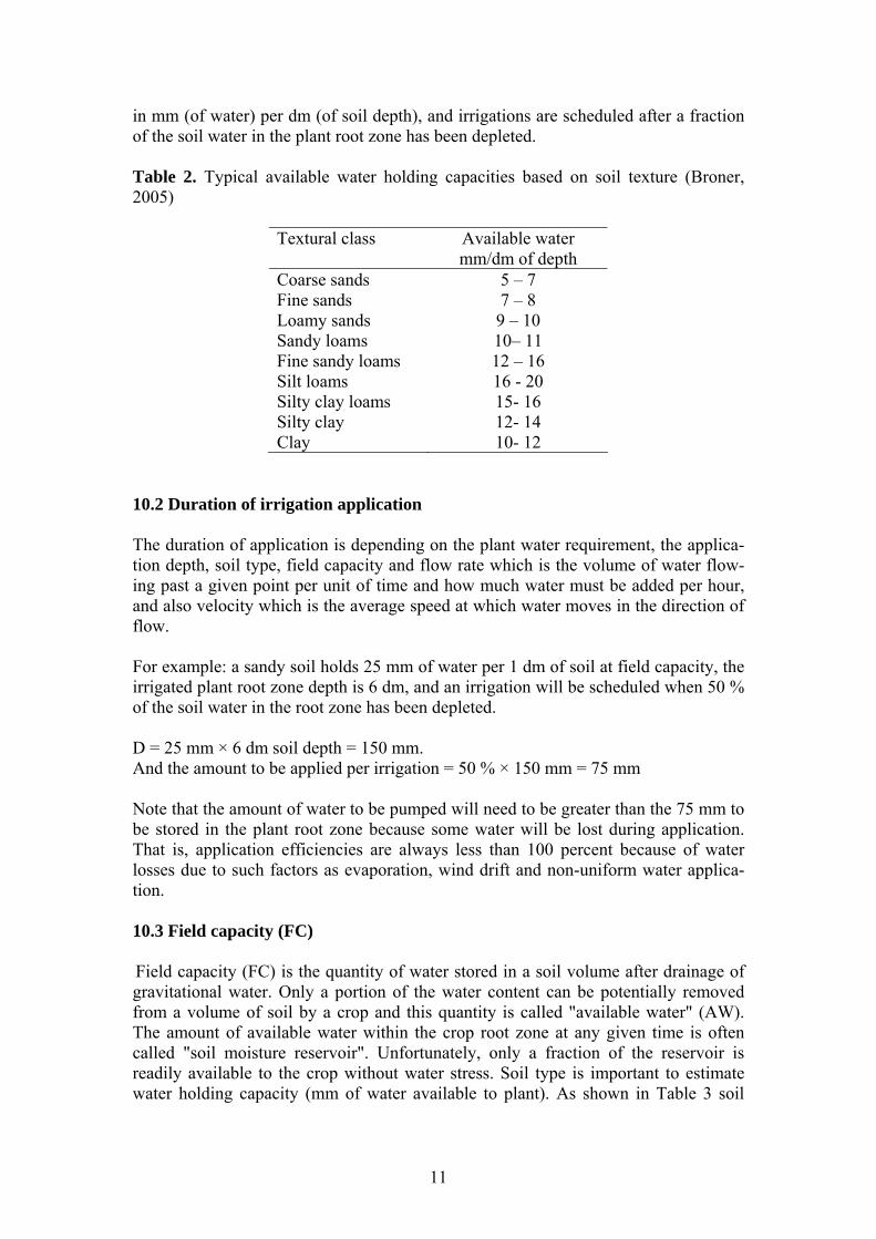
in mm (of water) per dm (of soil depth), and irrigations are scheduled after a fraction of the soil water in the plant root zone has been depleted. Table 2. Typical available water holding capacities based on soil texture (Broner, 2005)

Textural class Available water mm/dm of depth

Coarse sands 5 – 7 Fine sands 7 – 8 Loamy sands 9 – 10 Sandy loams 10– 11 Fine sandy loams 12 – 16 Silt loams 16 - 20 Silty clay loams 15- 16 Silty clay 12- 14 Clay 10- 12

10.2 Duration of irrigation application The duration of application is depending on the plant water requirement, the applica-tion depth, soil type, field capacity and flow rate which is the volume of water flow-ing past a given point per unit of time and how much water must be added per hour, and also velocity which is the average speed at which water moves in the direction of flow. For example: a sandy soil holds 25 mm of water per 1 dm of soil at field capacity, the irrigated plant root zone depth is 6 dm, and an irrigation will be scheduled when 50 % of the soil water in the root zone has been depleted.

D = 25 mm × 6 dm soil depth = 150 mm. And the amount to be applied per irrigation = 50 % × 150 mm = 75 mm

Note that the amount of water to be pumped will need to be greater than the 75 mm to be stored in the plant root zone because some water will be lost during application. That is, application efficiencies are always less than 100 percent because of water losses due to such factors as evaporation, wind drift and non-uniform water applica-tion. 10.3 Field capacity (FC) Field capacity (FC) is the quantity of water stored in a soil volume after drainage of gravitational water. Only a portion of the water content can be potentially removed from a volume of soil by a crop and this quantity is called "available water" (AW). The amount of available water within the crop root zone at any given time is often called "soil moisture reservoir". Unfortunately, only a fraction of the reservoir is readily available to the crop without water stress. Soil type is important to estimate water holding capacity (mm of water available to plant). As shown in Table 3 soil

11

texture influences the water holding capacity of soils shows the field capacity of dif-ferent soil texture. Heavy soils with slow infiltration properties are prone to water logging (Whitfield et al., 1986). A low hydraulic conductivity often means poor aeration. Phythophtora root rot occurs under poor drainage. Soil parameters influence the depth at which vine roots grow and amount of water held within the vine root zone. For example, sandy areas, due their relatively large grain size, have a low water holding capacity, whereas soils with higher clay content have a higher water-holding capacity. We can use soil samples to measure the level of soil water or its status, but soil sam-pling by itself does not provide forecast of the irrigation time and water amount of next irrigation (Heermann et al., 1990). Table 3. Values for available water holding capacity according to Jensen et al., (1990a, p.21) Texture class Field capacity

mm/dm Wilting point

mm/dm Available capacity

mm/dm Sand 12 4 8 Loamy Sand 14 6 8 Sandy Loam 23 10 13 Loam 26 12 15 Silt Loam 30 15 15 Silt 32 15 17 Silty Clay Loam 34 19 15 Silty Clay 36 21 15 Clay 36 21 15

11 Start of scheduling The goal of irrigation scheduling is to make the most efficient use of water and energy by applying the right amount of water to cropland at the right time and in the right place. Proper irrigation scheduling requires a lot of information about the soil and the crop. The soil properties can be very important parameter to determine the water status in the root zone, which is related to the amount of water. Also the crop infor-mation is important when we determine the water requirement.

To getting started with irrigation scheduling, there are two important factors which is shown below:

- Determine the time of irrigation. - Calculate water requirement.

11.1 Determine the time of irrigation Determine the time of irrigation means decide when we should supply the water to the field. The time of irrigation plays a crucial role for crop yield and water efficiency.

12

Adding water too late or too early means in both cases losing water and energy, and finally decreased crop yield. Therefore there are many techniques and technologies that can forecast the timing and amount of irrigation water to supply:

1) Monitoring the soil 2) Monitoring the crop 3) Monitoring the weather conditions

11.1.1 Monitoring the soil Monitoring the soil moisture status is one of the most important methods to establish the time for irrigation. Periodic observations of the soil water status can be used to adjust the calculated soil water depletion. Soil water can be measured by methods that determine the soil water content or the soil water potential. Soil water content is the amount of water per volume of soil or weight of dry soil. Soil water potential is the force necessary to remove the next increment of water from the soil (Shock, 2006). Methods used in monitoring soil water status are shown below:

- Tensiometer measurements - Nuclear methods - Hand feel and appearance of soil - Gravimetric soil moisture sampling - Electrical resistance blocks - Water budget approach - TDR (Time Domain Reflectometers)

All of these methods are used in the field, just the fourth one is a laboratory method.

11.1.1.1 Tensiometers A tensiometer is an instrument used to measure the soil water potential, which is re-lated of soil moisture status. A tensiometer consists of a manometer and a closed tube connected at the end with special ceramic tip. After irrigation, as soil moisture is depleted by evaporation or root extraction, the ten-siometers register increase in tension and properly interpreted, can help to forecast when the plant might begin to suffer stress. A tensiometer measures the soil water ten-sion that can be related to the soil water content as shown in Figure 1. The measured value indicate the energy that is needed to exert by the plant to extract water from the soil. Generally, soil water tension increases with decreased soil water content, this means high readings for dry soils and low for wet soils. Van der Gulik (2006) shows that, for most soil types, readings less than 10 cbars indicate a wet soil; above 50 cbars indicate a dry soil. The tensiometers are available in various lengths, allo-wing the monitoring of soil moisture tension at various depths. To install a tensiometer make sure that the ceramic tip of a tensiometer is soaked for 24 hours in a container of water. Preferably an algaecide prevent algae growth from clouding the water in the tensiometer column. Also make sure that the ceramic tip of the tensiometer has good contact with the surrounding soil.

13

Figure 1. A diagram of typical tension and water amount for sand, clay and loam soils. From Edward et al., ( 2001).

In general the tensiometer should be monitored at lest once or twice a week, and by plotting the reading on the graph it will be more helpful to see the change in the soil water tension. But with high soil water tension the tensiometer should monitored daily. The irrigation scheduling can be done with tensiometer by using trigger levels, taking into account different types of irrigation systems and soil types. Table 4 indi-cates the range the tensiometer should read to keep the soil moisture at optimum lev-els when using a drip irrigation system. For other irrigation systems normally higher levels are recommended before irrigation start. Table 4. Soil moisture range for drip/trickle and micro-jet system (Tam, 2006)

Soil moisture tension (cbars) Soil type Low (wet) High (dry)

Sand 10 15 Loamy sand 10 15 Sandy loam 15 20 Loam 25 30

With different irrigation systems the moisture level can be maintained by adjusting the set time and the length of time the zone is irrigated. If the soil is always wet or dry, adjust the amount of time the zone is irrigated to bring the soil moisture to the optimal level. Generally, tensiometers can be used in all types of soils if they are not too dry. When heavy clay soils dries, the tension often exceeds maximum reading (80 cbars),

The advantages of tensiometers are:

1) They are low cost. 2) They are easy to install and reasonable simple to maintain. 3) They can operate for long periods of time if properly maintained. 4) They can be easily adapted to automatic measurement by using pressure trans-

ducers or electric switch. 5) They can be operated in frozen soils with ethylene glycol.

14

The disadvantages are: 1) Tensiometers function to about 80 cbars, which is a small part of the entire

range of available water for most soils (no problem in sandy soil). Tensiome-ters are better suited for use on sandy soils, where they monitor most of the available moisture range. In heavy soils, large amounts of available moisture occur outside the detection limits of the tensiometer.

2) They measure soil water tension directly rather than soil water content (know-ledge of the soil water characteristic curve is required to determine water con-tent).

3) They display hysteretic behaviour. 4) They are subject to breakage during installation or by farming activities. 5) They require regular maintenance depending on the range of measurements. 6) They disturb the soil above the measurement point and can allow infiltration

of irrigation water or rainfall along the stem. 11.1.1.2 Nuclear methods Nuclear techniques depend on measuring the behaviour of sub-atomic particles in soils. Sub-atomic particles are released from a low-level radioactive source in the soil or on the surface of the soil. Changes in the properties of these particles or changes induced by these particles are then monitored. These methods require calibration for different soils since the behaviour of the particles does not necessarily depend on the presence of water alone. For irrigation management, the neutron probe is the most commonly used instrument of this type. The neutron probe is measuring soil water status, as it provides the opportunity of re-peated soil water measurements at the same location within the field. Neutron scat-tering was first successfully used from measuring soil water content in the 1950’s (Evett et al., 1995). The neutron probe must be calibrated to give the total volume of water per unit depth in the soil profile. With the neutron scattering method, a source of fast neutrons and a detector of ther-mal neutrons are employed. Fast neutrons are released in the soil from a radioactive source. The fast neutrons impact hydrogen atoms in the soil resulting in emissions of thermal neutrons. Thermal neutrons are then detected. Three processes are involved in the application: 1) fast neutron emission from a radioactive source; 2) moderation of the neutrons to thermal velocities by collisions in the soil medium and backscattering towards the instrument; 3) selective detection and counting of thermal neutrons at a point close to the source. Since most of the hydrogen atoms present in the soil are in water, this is very effective means of estimating soil content. Two energy neutron sources are used with this technique, americium-beryllium (Am-Be) and radium-beryllium (Ra-Be). Am-Be is the one used in most types of neutron probes (depth probe and surface probe) that are available commercially for soil water measurement. The depth probe is generally a small cylinder that can be lowered into the soil through an access tube to the depth at which the water content is to be deter-mined. The surface probe is placed directly on the surface of the soil and measures the average water content of the top few centimeters of soil. The readings obtained from both types of probes are averages of soil water in the volume of soil around the probe (approximately 150 mm in radius).

15

The neutron probe is a reliable method of observing changes in the soil water content. Neutron probe sites need to be installed in replications to account for the spatial varia-bility in soil conditions. Soil water content can be accurately measured with this de-vice. However, the neutron probe needs to be site calibrated. The neutron probe measures total water within the soil profile, depending on the soil type, plant available water varies as percentage of total water (approximately 50 percent for sand). The advantages of the neutron scattering method are:

1) It is non-destructive. 2) It is possible to obtain the profile of water content in soil. 3) Water can be measured in any phase. 4) The system can be automated for one site to monitor spatial and temporal soil

water. 5) Measurement is directly related to soil water.

The disadvantages are: 1) Cost is relatively high. 2) The measurement depends on the geo-chemical properties of the soil. 3) Care must be taken to avoid radiation hazard. 4) Proper calibration is needed. 5) Depth resolution is questionable (at near surface) 6) It is labour intensive.

11.1.1.3 Hand feel and appearance of soil Some methods are expensive and difficult to get, but there are other very cheap meth-ods like “hand feel method”. By this method we can estimate soil moisture by ob-taining a handful of soil and squeeze tightly. If it forms a ball, bounce three times lightly in your palm. The relative soil moisture can be determined for the different soils by using Table 5. This method, however, has some serious disadvantages:

1) it is non-quantitative and subjective, 2) it does not give any lead time for irrigation, 3) it is subject to misuse such as: only looking at the surface soil in a limited

area, Given these limitations, the “feel” method is not recommended as the sole means of irrigation scheduling, but should still be used as verification of other methods.

16

Table 5. Water availability for different soils, numbers in parentheses are available water content expressed as cm of water per 3 dm of soil depth. Based on Van der Gulik (2006)

Feel or appearance of soil Available water Sand Sandy Loam Loam/Silt Loam Clay Loam/Clay

> 100 % Free water ap-pears when soil is bounced in hand

Free water is re-leased with kneading

Free water can be squeezed out

Puddles; free water forms on surface

100 % Upon squeezing, no free water appears on soil, but wet outline of ball is left on hand (2.5 cm)

Appears very dark. Upon squeezing, no free water ap-pears on soil, but wet outline of ball is left on hand. Makes short rib-bon. (3.75 cm)

Appears very dark. Upon squeezing, free water appears on soil, but wet outline of ball is left on hand. Will ribbon about 2.5 cm. (5 cm)

Appears very dark. Upon squeezing, no free water appears on soil, but wet outline of ball is left on hand. Will ribbon about 5 cm. (7.5 cm)

75 - 100 % Tends to stick together slightly sometimes forms a weak ball with pressure. (2 -2.5 cm)

Quite dark. Forms weak ball, breaks easily. Will not slick. (3 – 3.75 cm)

Dark coloured. Forms a ball, is very pliable, slicks readily if high in clay. (3.75 – 5 cm)

Dark coloured. Easily ribbons our between fingers, has slick feeling (4.75 – 6.25 cm)

50 – 75 % Appears to be dry, will not form a ball with pressure. (1.25 – 2 cm)

Fairly dark. Tends to form ball with pressure but sel-dom holds to-gether. (2 – 3 cm)

Fairly dark. Forms a ball somewhat plastic, will sometimes slick slightly with pressure. (2.5 – 3.75 cm)

Fairly dark. Forms a ball, ribbons out be-tween thumb and forefinger. (3 – 4.75 cm)

25 – 50 % Appears to be dry, will not form a ball with pressure. (0.5 – 1.25 cm)

Light coloured. Appears to be dry, will not form a ball (1 – 2 cm)

Lightly coloured. Somewhat crumbly, but holds together with pressure. (1.25 – 2.5 cm)

Slightly dark. Some-what pliable, will ball under pressure. (1.5 – 3 cm)

0 – 25 % Dry, loose, sin-gle- grained, flows through fingers. (0 – 0.5 cm)

Very slightly col-oured. Dry loose, flows through fin-gers. (0 – 1 cm)

Slightly coloured. Pow-dery, dry sometimes slightly crusted, but easily broken down into powdery condition (0 – 1.25 cm)

Slightly coloured. Hard, baked, cracked, sometimes has loose crumbs on surface. (0 – 1.5 cm)

11.1.1.4 Gravimetric soil moisture sample Is traditional method and consists of using a soil probe or auger to remove samples for weighing. The weighing is done before and after drying in an oven at 105o C for twenty- four hours or longer. The volumetric water content of the soil is computed as follows:

w

b

d

dw

www

ρρ

θ ⋅−

= (1)

where θ is the soil water content (cm3/cm3), ww is the weight of the soil sample at wet or field condition (g), wd is the weight of the soil simple after drying (g), ρb is the dry

17

bulk density of the soil (g/cm3), ρw is the density of water (1.0 g/cm3). When using this method, it is necessary to know the bulk density of the soil. The size and number of samples affect the final result (Hillel, 1980). 11.1.1.5 Electrical resistance blocks Electrical resistance block is another method used to measure soil water to help de-cide when irrigation is needed. Electrical resistance block reading can also help elimi-nate irrigation when soil water is adequate (Alam and Rogers, 2001). Avoiding unnecessary irrigation will also help prevent environmental degradation and loss of nitrogen (nitrate) fertilizer. Electrical resistance blocks are installed during the growing season at several soil depths and determine the amount of water at each depth. Soil water readings can be used to schedule irrigations or assist with checkbook methods. The electrical resistance varies between the electrodes according to water content. Higher soil water content gives less resistance. The blocks must be installed in the field after the crop has emerged. To get successful installation we must make sure the black has good contact with the soil at the bottom. The location of the block in the field is depending on the kind of irrigation system. When installing the block it is better to avoid low or high spots and changing slopes, and the area must be at a represent plant population. It is very important when we installing the block in the field considering the effective root zone of the crop, to placing the block at the right depth. Alam and Rogers (2001) shows the effective root zone for deep rooting crops such as corn, sorghum, alfalfa and wheat can be as much as 180 cm. The active root depth is the upper portion of the root zone where plants get most of their water. However, the most active portion is above 90 to 120 cm. Water at depth greater than this may be lost to deep percolation. The management of active root zone can be done by using two blocks. The upper block placed at about one-fourth to one-third depth of the root zone. While the lower block will be at two-thirds to three-fourths of the active root zone. This means block depth would be 30 to 45 cm for the shallow block and 75 to 90 cm for deep block (Figure 2). In some cases the block should not be placed as deep as crop root. For example sugar, soybeans and field beans have effective root zone between 75-90 cm, so the suggestion of block installation depth for two is 30 and 60 cm. To getting started with irrigation scheduling by using block resistance method we must have information about the soil water-holding capacity to make full use of the data obtained from gypsum blocks. The management allowable depletion level is 50 percent of total available water for the soil types. The irrigation may be started before reaching this level to avoid stress for the area that receives water later. Different soils have different water holding capacity and different readings. Sandy loams with a water holding capacity of 15 mm per dm soil depth turn on the water at a meter reading indicating tension 60 centibars. On clay loams and silty clay loams or soils with water holding capacity of 20 mm per dm or greater, start irrigation at 70 to 80 centibars.

18

Figure 2. Location of electrical resistance blocks in relation to the active root zone. A is 1/4 to 1/3 of active root zone; B is 2/3 to 3/4 of active root zone. Based on Alam and Rogers (2001). 11.1.1.6 Water budget approach Water budget method is based on climate data. In a water budget, the crop root zone is visualized as a reservoir of available water. There are two factors adding to the reser-voir, rainfall and irrigation. Water is removed from reservoir through crop water con-sumption, transpiration, and evaporation from the soil surface. Generally, water budget is like a bank account, irrigation and rainfall are deposits to the account and daily crop water use is a withdrawal from the account. Available soil moisture stored in the root zone is then like the balance in the account. With this method we must cal-culate how much water is being taken out of the soil to determine how much water has to be added to keep the moisture balance within the optimal range. The main re-quirement for scheduling irrigation with the water budget approach is that you have accurate estimates of daily crop water use. The daily crop water use can be estimated from percent crop cover and maximum evapotranspiration rate derived from climatic data (Tan, 1990). As an example Tan (1990) has used water budget approach for scheduling irrigation of tomatoes. The type of the soil was loamy sand. In the study, the root depth before flowering was 30 cm and after flowering 60 cm. Maximum total water available and allowable depletion can be calculated. To start to calculate maximum total water available in the root zone of tomatoes, we must know the available water capacity of the soil type that we have in our field. From Table 6, available water capacity of loamy sand is 7- 10 mm/dm. The total maximum available water is calculated at 30 cm and 60 cm depths as following: Maximum available water = appropriate available water × rooting depth Available water before flowering = 10 mm cm-1 × 3 dm = 30 mm, available water after flowering = 10 mm cm-1 × 6 dm = 60 mm

19

Table 6. Ranges in available water capacity and intake rate for various soil textures (Tan and Layne, 1990)

Soil texture Available water capacity mm of water/dm of soil

Intake rate mm/hr

Sands 5 – 8 12 – 20 Loamy sand 7 – 10 7 – 12 Sandy loam 9 – 12 7 – 12 Loam 13 – 17 7 – 12 Silt loam 14 – 17 4 – 7 Silty clay loam 15 – 20 4 – 7 Clay loam 15 – 18 4 – 7 Clay 15 – 17 2 – 5

As we know the available soil water for the crop and the allowable depletion should not exceed 50 % for the total available water. So we can calculate the allowable water depletion by multiply 50 % by available soil water. Allowable water depletion before tomato is flowering = 50 % × 30 mm = 15 mm Allowable water depletion after tomato is flowering = 50 % × 60 mm = 30 mm 11.1.1.7 TDR (Time Domain Reflectometry) TDR is a volumetric field methods and a dielectric method. The instrument is used to measure soil water content, bulk electrical conductivity, and rock mass deformation. TDR determinations involve measuring the propagation of electromagnetic waves or signals. Propagation constants for electromagnetic waves in soil, such as velocity and attenuation, depend on soil properties, especially water content and electrical conduc-tivity. The propagation of electrical signals in soil is influenced by soil water content and electrical conductivity. The dielectric constant, measured by TDR, provides a good measurement of this soil water content. A TDR instrument requires a device capable of producing a series of precisely timed electrical pulses with a wide range of high frequencies. The pulses travel along a transmission line (TL) that is built in a coaxial cable and a probe. The TDR probe usually consists of 2-3 parallel metal rods that are inserted into the soil acting as waveguides in a similar way as an antenna used for television reception. At the same time, the TDR instrument uses a device for measuring and digitizing the energy (voltage) level of the TL at intervals down to around 100 picoseconds. When the electromagnetic pulse traveling along the TL finds a discontinuity (i.e., probe-waveguides surrounded by soil) part of the pulse is reflected. This produces a change in the energy level of the TL. Thereby the travel time is determined by analyzing the digitized energy levels (Muñoz-Carpena, 2004). Time domain reflectometry lends itself to automated monitoring of soil water content (Heimovaara and Bouten, 1990; Evett, 1994) with numbers of soil probes rising to the several tens or even hundreds in a single measurement system.

20

In arid areas there are two uncertainties remain for use of TDR sensors. First, TDR sensors have not previously been used in hyper-arid environments. Second, TDR sensors depend largely on soil properties, soil salinity and soil temperature (Dalton et al., 1984; Wraith and Or, 1999).

Advantages - Accuracy - Soil specific-calibration is usually not required - Easily expanded by multiplexing - Wide variety of probe configurations - Minimal soil disturbance - Relatively insensitive to normal salinity levels - Can provide simultaneous measurements of soil electrical conductivity

Drawbacks - Relatively expensive equipment due to complex electronics - Potentially limited applicability under highly saline conditions or in highly

conductive heavy clay soils - Soil-specific calibration required for soils having large amounts of bound water

(i.e. those with high organic matter content, volcanic soils etc.) - Relatively small sensing volume (about 3 cm radius around length of waveguides) 11.1.2 Monitoring the crop Irrigation scheduling methods, it can be used by concentrate on the water status of the crop root zone profile. As direct measurements of plant water status (leaf water potential) can also be used for scheduling irrigation. (Heermann et al., 1990). In addition to, or as an alternative to monitoring the soil, it is possible to monitor the water status of the plants. As in the case of soil moisture, numerous methods have been proposed over the year to monitor the state of water in the plant. Included among these are techniques to estimate transpiration using excised leaves, observations of stomatal aperture, monitoring stem diameter, pressure-cell and psychrometric meas-urements of leaf water potential, and more. Perhaps the most comprehensive are measurements of total plant transpiration and photosynthesis, using portable tents with transparent plastic walls. There are also practical methods as the monitoring of crop canopy temperature by remote sensing with an infrared radiation thermometer (Jackson, 1982). Still the most common way to monitor the crop is by the tried and true method of direct visual inspection An experienced agronomist or farmer who knows his crop can detect early signs of thirst by the appearance of the foliage, especially during the period of peak transpiration demand (usually at midday). Another method to determining the irrigation time is called Crop Water Stress Index (CWSI). This method can be used to measure crop water status and also to improve irrigation scheduling. The crop water stress index (CWSI), derived from canopy-air temperature differences versus the air vapour pressure deficit (AVPD), was found to

21

be a promising tool for quantifying crop water stress (Jackson et al., 1981; Idso et al., 1982; Jackson, 1982).

CWSI = llaculac

llacac

TTTTTTTT

)()()()(

−−−−−− (2)

where (Tc-Ta) is the measured temperature difference. Tc= the canopy temperature (oC). Ta = the air temperature (oC). ll = the non- water stressed baseline (lower baseline) ul = the non-transpiring upper baseline.

11.1.3 Monitoring the weather This method can give meteorological information which is used to measure the amount of evapotranspiration as it varies over time and to set the quantity of irrigation accordingly (Hillel, 1990). The timing of irrigation can then by determined in refer-ence to the soil’s effective storage capacity or its moisture tension (or residual wet-ness), or in reference to the status of the crop. 11.2 Crop water requirement Calculation of crop water requirements and crop irrigation requirements can be car-ried out from basic information from the crops selected and should include, average planting date and average harvesting data (FAO, 1996). Standard information on crop coefficient, rooting depth, depletion level and yield response factors, and length of individual growth stages are needed. The water requirements are different from one crop to another. Although growing crops are continuously using water, the rate of water use depends on (1) the kind of crop, (2) the degree of maturity and (3) atmospheric condition, such as radiation, tem-perature, wind, and humidity. The rate of growth at different soil water contents varies with different soils and crops. During early stages of growth the water needs are gen-erally low, but they increase rapidly during the maximum growing period to the frui-ting stage. During the later stages of maturity, water use decreases as the crops ripen (Schwab et al., 1995). 12 Evapotranspiration definitions Evapotranspiration (ET) is the sum of evaporation and plant transpiration. Evapora-tion accounts for the movement of water to the air from sources such as the soil, can-opy interception, and water bodies. Transpiration accounts for the movement of water within a plant and the subsequent loss of water as vapour through stomata in its leaves. Evapotranspiration plays an important role in the water cycle. The driving force of evaporation process is the difference between the water vapour pressure at the evaporating surface and vapour pressure of the surrounding atmos-phere. As the evaporation is requiring energy to change the water molecules from liq-uid to vapour, the source of this energy is solar radiation and temperature. Some fac-tors effecting evaporation process are wind speed, solar radiation, air temperature, air humidity, water available and the degree of shading of the crop canopy.

22

With transpiration the driving force is the difference between water vapour inside the leaf and the atmosphere. Factors effecting transpiration are solar radiation, wind speed, air humidity, air temperature, crop characteristics and soil water content (Allen et al., 1998). 13 Factors affecting evapotranspiration The amount of water that plants transpire varies greatly geographically and over time. There are a number of factors that determine transpiration rates:

Temperature: Transpiration rates go up as the temperature goes up, especially during the growing season, when the air is warmer due to stronger sunlight and warmer air masses. Higher temperatures cause the plant cells which control the openings (sto-mata) where water is released to the atmosphere to open, whereas colder temperatures cause the openings to close.

Relative humidity: As the relative humidity of the air surrounding the plant rises the transpiration rate falls. It is easier for water to evaporate into dryer air than into more saturated air.

Wind and air movement: Increased movement of the air around a plant will result in a higher transpiration rate. This is somewhat related to the relative humidity of the air, in that as water transpires from a leaf, the water saturates the air surrounding the leaf. If there is no wind, the air around the leaf may not move very much, raising the humidity of the air around the leaf. Wind will move the air around, with the result that the more saturated air close to the leaf is replaced by drier air.

Soil-moisture availability: When moisture is lacking, plants can begin to senescence (premature ageing, which can result in leaf loss) and transpire less water.

Type of plant: Plants transpire water at different rates. Some plants which grow in arid regions, such as cacti and succulents, conserve precious water by transpiring less water than other plants.

14 Determining evapotranspiration (ET) When we start to determine evapotranspiration process, we must understand that when the plant is small, the main process causing loss of water from the soil to the atmosphere is evaporation process. But after the plant has grown up and developed, and completely covers the soil then the main process is transpiration. The evaporation process can be determined by the fraction of the solar radiation reaching the soil sur-face. This fraction decreases over the growing period as the crop develops and the crop canopy shades more and more the ground area. There are more or less accurate methods for estimating ET. The selection of method depends on the availability of data for use in calculating ET. To calculate actual ET there are some methods that can be used in this way as following:

23

14.1 Soil water balance Evapotranspiration can be determined by using the soil water balance method by measuring the various components of the soil water balance (Heermann, 1985). The equation can be written as;

ET = I + P – RO – DP + CR ± ∆ SF ± ∆ SW (3) where I is the irrigation water supplied (mm), P is the rainfall, RO is surface runoff, DP is the deep percolation which recharge water table. CR is the capillary rise, the capillary rise is important in case shallow water table. ∆ SF is subsurface flow in (SFin) or out flow (SFout) of the root zone. ∆ SW is change in the soil water content. In this approach evapotranspiration is determined as a residual term and, all the other components given in the above equation have to be either measured or estimated. Generally it is accepted that the water balance approach yield an acceptable degree of error in evapotranspiration estimation if performed on longer periods e.g. 10 days or a month. One of the widely used techniques on basis of the water balance approach is the lysimeter method. A lysimeter is an artificial soil volume which can be used to deter-mine the actual evaporation in a natural environment by accurately measuring the other components of the water balance; i.e. precipitation, soil moisture storage and deep percolation. 14.2 Energy balance and microclimatological methods This method is based on the determination of energy which is used in evaporation of water. Because the evaporation of water requires large amounts of energy, as the en-ergy arriving at the surface must equal the energy leaving the surface for the same time period (Allen et al., 1998). The equation for an evaporation surface can be written as:

Rn-G-λET-H = 0 (4) where Rn is the net radiation, H the sensible heat, G the soil heat flux and λ ET the latent heat fluxes. There are different equations used to estimate the potential evapotranspiration with good accuracy, especially in arid climates, like Penman (1948, 1963) equation. Fac-tors such as data availability, the intended use, and the time scale required by the problem must be considered when choosing the evapotranspiration calculation tech-nique (Shih et al., 1983). 15 Reference evapotranspiration Reference evapotranspiration refers to the expected water use from a uniform green cover crop surface such as grass. There have been traditionally two types of reference crops (grass and alfalfa). But some times alfalfa has been preferred as reference crop because alfalfa has aerodynamic roughness closer to most field crops. There are the

24

several methods used to estimate reference evapotranspiration from reference crops. Actual crop water use is generally less and is determined by using a crop coefficient which relates actual evapotranspiration (ETc) to ETo. The calculation of reference evapotranspiration is a very common method used to calculate the crop water requirement, which is a need for irrigation scheduling design. The reference evapotranspiration rate from a reference surface (hypothetical grass or alfalfa surface with specific characteristics), with an assumed crop height of 0.12 m, with a fixed surface resistance of 70 sm-1 and an albedo of 0.23 is closely resembling the evapotranspiration from an extensive surface of green grass of uniform height, actively growing, well-watered, and completely shading the ground (Irmak and Ha-man, 2003). Both grass and alfalfa have been used as reference crop, but researchers generally agree that a clipped grass provides a better representation of reference evapotranspi-ration than does alfalfa. This is mainly because of two reasons, first the characteristics of the grass are better known and defined, and the second reason is that the grass crop has more planting areas than alfalfa throughout the world and measured evapotranspi-ration rates of grass are more readily available and accessible as compared to the measured alfalfa evapotranspiration. The following nomenclature is often used for reference evapotranspiration data (Van der Gulik, 2001): ETo – evapotranspiration calculated using grass as the reference crop ETr – evapotranspiration calculated using alfalfa as the reference crop ETp – evapotranspiration measured from a pan or atmometer. Reference evapotranspiration can be calculated from meteorological data by using different methods, like FAO-Penman-Monteith, Pan Evaporation and Blaney-Criddle. 16 Calculation of reference evapotranspiration Most of methods used to calculate reference evapotranspiration require some climate data and geographic information as well to calculate ETo. Different methods have dif-ferent procedures. The explanation of some of these methods is shown below. From reference evapotranspiration we can calculate the actual evapotranspiration ETc for different crops by multiplying reference evapotranspiration in crop coefficient Kc as is show in next equation.

ETc = ETo × Kc (5) - ETc actual evapotranspiration [mm] - ETo reference evapotranspiration [mm] - Kc crop coefficient ( some crop characteristic through different growth stage)

25

16.1 FAO-Penman-Monteith method Penman-Monteith equation is a combination equation that has generally been accepted as a scientifically sound formulation for estimation of reference ETo. This equation is expressed as combined function of radiation, maximum and minimum temperature, vapour pressure, and wind speed (Hatfield, 1990). The Penman-Monteith method is considered to offer the best results with minimum possible error in relation to a living grass reference crop. Penman-Monteith combination method is new standard for reference evapotranspira-tion with calculation of various parameters. By defining the reference crop as a hypothetical crop with an assumed height of 0.12 m having a surface resistance of 70 sm-1 and an albedo of 0.23, closely resembling the evaporation of an extension surface of green grass of uniform height, actively growing and adequately watered (Allen et al. 1998). The expression of the Penman-Monteith equation is shown below. The Penman equa-tion is combined to different equations, each equation has expression of some factors used to determine ETo.

Penman method has derived from combination equation; the equation 6 is introducing resistance factors. The resistance factor distinguishes between aerodynamic resistance and surface resistance. The aerodynamic resistance describes the resistance from the vegetation upward and involves friction from air blowing over vegetative surfaces. The surface resistance describe the resistance of vapour flow through stomata opening, total leaf area and soil surface.

λET =

⎟⎟⎠

⎞⎜⎜⎝

⎛++Δ

−+−Δ

a

s

a

aspan

rr

ree

cpGR

1

)()(

γ (6)

where Rn is the net radiation, G is the soil heat flux, (es - ea) represents the vapour pressure deficit of the air, pa is the mean air density at constant pressure, cp is the spe-cific heat of the air, ∆ represents the slope of the saturation vapour pressure tempera-ture relationship, γ is the psychrometric constant, and rs and ra are the (bulk) surface and aerodynamic resistances. The aerodynamic resistance is the determination of transfer of heat and water vapour from the evaporating surface into the air above the canopy.

ra = z

oh

h

om

m

uKz

dzIn

zdz

In

2

⎥⎦

⎤⎢⎣

⎡ −⎥⎦

⎤⎢⎣

⎡ −

(7)

26

where ra aerodynamic resistance [sm-1] zm height of wind measurements [m] zh height of humidity measurements [m] d zero plane displacement height [m] zom roughness length governing momentum transfer [m] zoh roughness length governing transfer of heat and vapour [m] K von Karman’s constant, 0.14 [-] uz wind speed at height z [m s-1] The bulk surface resistance describe the resistance of vapour flow through the tran-spiring crop and evaporation soil surface when the vegetation does not completely cover the soil surface.

rs = active

l

LAIr

(8)

where rs surface resistance [s m-1] rl bulk stomatal resistance of the well-illuminated leaf [s m-1] LAIactive active (sunlit) leaf area index [m2 (leaf area) per m2 (soil surface)] After the Penman method is updated by FAO in May 1990, the Penman Monteith

equation is written as the following:

ETo = )34.01(

)(273

900)(408.0

2

2

uy

eeuT

yGR asn

++Δ

−+

+−Δ (9)

ETo reference evapotranspiration [mm day-1] Rn net radiation at the crop surface [MJ m-2 day-1] G soil heat flux density [MJ m-2 day-1] T mean daily air temperature at 2 m height [oC] u2 wind speed at 2 m height [m s]-1

es saturation vapour pressure [KPa] ea actual vapour pressure [KPa] es – ea saturation vapour pressure deficit [KPa] ∆ slope vapour pressure curve [KPa oC-1] γ psychrometric constant [KPa oC-1]

The equation uses standard climatological records of solar radiation (sunshine), air temperature, humidity and wind speed. To ensure the integrity of computations, the weather measurement should be made at 2 m (or converted to that height) above an extensive surface of green grass, shading the ground and not short of water. By using the Penman equation we can calculate ETo for the whole year (as shown in Figure 3). The advantage of Penman method is that the method is reasonable accurate and that data are available from meteorological stations. The disadvantage of this method is that, estimated potential ET for reference crop, actual ET for various crops estimated with crop coefficients and Kc varies with local conditions, also often the data needed are not available.

27

ETo Penman of South Libya in 2003

2,77 3,855,78

7,649,12

10,47 9,76 8,837,69

6,254,28

2,55

11,35

14,9

18,9

23,55

27,65

31,6 31 30,4528,5

25,2

19,65

11,85

0

5

10

15

20

25

30

35

Janu

ary

Febr

uary

Mach

April

MayJu

ne July

Augus

t

Septem

ber

Octobe

r

Novem

ber

Decem

ber

Eto mmMean T

Figure 3. ETo graph by Penman method for southern Libya in 2003 (own cal-culation).

16.2 Pan evaporation method The most practical method for determining reference evapotranspiration ETo is the pan evaporation method. This approach combines the effects of temperature, humid-ity, wind speed and sunshine.

The evaporation from the pan is very near to evapotranspiration of grass that is taken as an index of ETo for calculating actual evapotranspiration ETc. The pan direct read-ings (Epan) are related to the ETo with the aid of the pan coefficient (Kpan), which depends on the type of pan, its location (surrounding with or without ground cover vegetation) and the climate (humidity and wind speed). ETo = Epan × Kpan (10) From ETo we can calculate crop water requirement (ETc) by determining the specific pan crop coefficient (Kc). To start to determine pan Evaporation (Epan) we must understand how we can use this method. Actually, there are different types of pans used to determining the evapora-tion rate. The most common types are circular pan or square pan. 16.2.1 Class A pan (Circular Pan) This kind of pan is very common to determining evaporation rate. The circular pan is usually 120.7 cm in diameter and 25 cm deep. It is made of galvanized iron or Monel metal (0.8 mm). The pan is mounted on a wooden open frame platform which is 15 cm above ground level. The soil built up to within 5 cm of the bottom of the pan. The pan must be level.

28

The pan is filled with water to 5 cm below the rim, and the water level should be not allowed to drop to more than 7.5 cm below the rim. The water should be regularly renewed, at least weekly, to eliminate extreme turbidity. The pan, if galvanized, is painted annually with aluminium paint. Screens over the pan are not a standard requirement and should preferably not be used. Pans should be protected by fences to keep animals from drinking (Allen et al., 1998). The site should preferably be under grass, 20 by 20 m, open on all sides to permit free circulation of the air. It is preferable that stations be located in the center or on the leeward side of large cropped fields. Pan readings are taken daily in the early morning at the same time that precipitation is measured. Measurements are made in stilling well that is situated in the pan near one edge. The stilling well is a metal cylinder of about 10 cm in diameter and some 20 cm deep with a small hole at the bottom. 16.2.2 Class B pan, (Square pan, Sunken Colorado Pan) The square pan is 92 cm square and 46 cm deep, made of 3 mm thick iron, placed in the ground with rim 5 cm above the soil level. Also, the dimensions 1 m square and 0.5 m deep are frequently used. The pan is painted with black tar paint. The water level is maintained at or slightly below ground level, i.e., 5 -7.5 cm below the rim. The measurements are taken similarly to those for the circular pan. The siting and environment requirements are also similar to those for circular and square pan. Some-times the square pan is preferred in crop water requirement studies, as these pans gives a better direct estimation of reference evapotranspiration than does the circular pan. The disadvantage is that maintenance is more difficult and leaks are not always visible.

So we can calculate the reference evapotranspiration (ETo) by multiplying pan evapo-ration (Epan) with pan coefficient (Kpan) as shown in equation (10). Kpan is the special coefficient to adjust the Epan to reference evapotranspiration; this coefficient is depending on the type of pan if it is circular or sunken pan, pan envi-ronment (fallow or cropped), wind speed and humidity. Pan evaporation method is real-time evaporation method and relatively easy. The dis-advantage of this method is that the data are influenced by pan placement and type, as water in pan stores and releases water differently than crop. 16.2.3 Pan Coefficient (Kpan) The pan coefficient is used to adjust the pan evaporation measurement. There are dif-ferent pan coefficients. The selecting of pan coefficient is depending on the type of pan and the size and state of the upwind buffer zone (fetch) and also the ground cover in the field, as also humidity should be checked. The siting of the pan and the pan en-vironment also influence the results, for instance if the pan is placed in fallow rather than cropped fields.

29

This situation was considered by Allen et al. (1998) in two cases; the first case where the pan was sited on short green grass cover and surrounded by fallow soil and the second case where the pan was sited on fallow soil and surrounded by green crop. These cases are affecting the water vapour, because the first case the air contains more vapour.

There are special tables showing pan coefficient (Kpan) for both circular pan and square pan, for different pan siting and environment and different levels of mean rela-tive humidity and wind speed, for more details see Allen et al. (1998). As an example of the use of pan coefficient table, if the daily pan evaporation meas-ured was 8.5 mm with pan class A, the pan was located in a grassed area with about 100 m of grass surrounding the pan, daily wind speed was strong (estimated to be more than 5 m/s, and humid conditions prevailed (daily minimum relative humidity was greater than 40%, as typical of most days)), Kpan would be read as 0.8. ETo would then be calculated as the multiple of 0.8 times 8.5 mm/day, which equals 6.8 mm/day. To calculate typical pan coefficient (Kpan) there are some equations presented as fol-lowing bellow. These equations are used to calculate Kpan. pan coefficient equation of circular pan where pan is placed with green fetch:

Kpan = 0.108 – 0.0286 u2 + 0.0422 ln(FET) + 0.1434 ln(RHmean) – 0.000631 [ln(FET)]2 ln(RHmean) (11)

pan coefficient equation of circular pan where pan is placed with dry fetch: Kpan = 0.61 + 0.00341 RHmean – 0.000162 u2 RHmean – 0.00000959 u2 FET + 0.00327 u2 ln(FET) – 0.00289 u2 ln(86.4 u2) – 0.0106 ln(86.4 u2) ln(FET) + 0.00063 [ln(FET)]2ln(86.4u2) (12)

pan coefficient of square pan where pan is placed with green fetch: Kpan = 0.87 + 0.119 ln(FET) – 0.0157 [ln(86.4 u2)]2 ln(86.4u2) ln(FET) RHmean (13)

pan coefficient of square pan where pan is placed with dry fetch: Kpan = 1.145 – 0.080 u2 + 0.000903(u2)2 ln(RHmean) – 0.0964 ln(FET) + 0.0031 u2 ln(FET) + 0.0015[ln(FET)]2ln(RHmean) (14)

where Kpan is pan coefficient, u2 average daily wind speed at 2 m height (m s-1) RHmean average daily relative humidity [%] = (RHmax + RHmin)/2 FET fetch, or distance of the identified surface type ( grass or short green agri-culture crop and dry crop or bare soil)

For example: measured pan evaporation data from the field were 8.2, 7.5, 7.6, 6.8, 7.6, 8.9 and 8.5 mm/day and the circular pan is installed in a green area, the wind speed was 1.9 m/s and mean relative humidity was 73 %. Determine the reference evapotranspiration during these 7 days. The pan coefficient was 0.85 which is calcu-lated from equation (11), so reference evapotranspiration is computed as following:

30

ETo = Epan × Kpan, Kpan = 0.85 Ep of the first day = 8.2 mm/day. ETo = 8.2 × 0.85 = 6.97 mm

By the same procedure we can calculate reference evapotranspiration of the other days. By pan evaporation Class A method the reference evapotranspiration can be calcu-lated for the whole year, as shown in the Figure 4.

ETo by Pan evaporation Class A (south Australia in 2005)

-50

0

50

100

150

200

250

300

0 2 4 6 8 10 12 14

Months

Average Temp

Average Wind Km/day

ETo mm

Total rainfall mm/month

Figure 4. The reference evapotranspiration for Renmark weather station in Australia 2005 (own calculation). Data obtained from web site of Depart-ment of Primary Industries and Resources, South Australia (PIRSA, 2007).

The pan evaporation is a practical method to estimate reference evapotranspiration. It is also reported that pan evaporation is a more satisfactory method of estimating ref-erence crop evapotranspiration than other methods for rice (Azhar et al., 1992). 16.3 Blaney-Criddle method The Blaney-Criddle equation is one of the simplest methods for estimating reference evapotranspiration by using measured data on temperature only. The Blaney-Criddle is not very accurate. Brouwer et al. (1986) shows that this method is less accurate: in windy, dry, and sunny areas where the ETo is up to some 60 % (underestimated), while in calm, humid, clouded areas, the ETo is up to some 40 %. (Overestimated) The Blaney-Criddle equation is only recommended for purpose of evapotranspiration estimation based on determinations of mean temperature. The formula is shown in equation 15: To determine the mean temperature we need the daily maximum and minimum tem-perature. The Blaney-Criddle method always refers to mean monthly values, both for the temperature and the ETo. If for example, it is found that mean temperature in

31

March is 28 oC, it means that during the whole of March the mean daily temperature is 28 oC (Brouwer et al., 1986). The calculation of maximum and minimum tempera-ture is shown in equations 16 and 17:

ETo = p(0.46 T mean + 8) (15)

where ETo is reference crop evapotranspiration (mm/day) T mean = mean daily temperature (oC) p = mean daily percentage of annual daytime hours

T max = monththeofdaysofnumber

monththeduringvaluesTallofsum max (16)

T min = monththeofdaysofnumber

monththeduringvaluesTallofsum min (17)

T mean = 2

minmax TT + (18)

To determine the mean daily percentage of annual daytime hours (P) there is a special table which is presented below. To use Table 7 we must have some information about latitude of the area (the number of degrees north or south of the equator). Table 7. Mean daily percentage of annual daytime hours for different latitude (Brouwer et al., 1986)

North Jan Feb Mar Apr May June July Aug Sept Oct Nov Dec Latitude South July Aug Sept Oct Nov Dec Jan Feb Mar Apr May June

60o 0.15 0.20 0.26 0.32 0.38 0.41 0.40 0.34 0.28 0.22 0.17 0.13 55 0.17 0.21 0.26 0.32 0.36 0.39 0.38 0.33 0.28 0.23 0.18 0.16 50 0.19 0.23 0.27 0.31 0.34 0.36 0.35 0.32 0.28 0.24 0.20 0.18 45 0.20 0.23 0.27 0.30 0.34 0.35 0.34 0.32 0.28 0.24 0.21 0.20 40 0.22 0.24 0.27 0.30 0.32 0.34 0.33 0.31 0.28 0.25 0.22 0.21 35 0.23 0.25 0.27 0.29 0.31 0.32 0.32 0.30 0.28 0.25 0.23 0.22 30 0.24 0.25 0.27 0.29 0.31 0.32 0.31 0.30 0.28 0.26 0.24 0.23 25 0.24 0.26 0.27 0.29 0.30 0.31 0.31 0.29 0.28 0.26 0.25 0.24 20 0.25 0.26 0.27 0.28 0.29 0.30 0.30 0.29 0.28 0.26 0.25 0.25 15 0.26 0.26 0.27 0.28 0.29 0.29 0.29 0.28 0.28 0.27 0.26 0.25 10 0.26 0.27 0.27 0.28 0.28 0.29 0.29 0.28 0.28 0.27 0.26 0.26 5 0.27 0.27 0.27 0.28 0.28 0.28 0.28 0.28 0.28 0.27 0.27 0.27 0 0.27 0.27 0.27 0.27 0.27 0.27 0.27 0.27 0.27 0.27 0.27 0.27

32

Table 8. Calculation result of reference evapotranspiration of dry climate (Libya-Sebha) using Blaney-Criddle method (own calculation)

Month Maximum temperature

oC

Minimum temperature

oC

Mean tem-perature oC

Latitude ETo mm

January 17.7 5.0 11.35 0.33 4.4 February 22.1 7.7 14.9 0.25 3.7

March 26.0 10.5 18.25 0.27 4.4 April 31.6 15.5 23.55 0.29 5.5 May 36.0 19.3 27.65 0.31 6.4 June 40.0 23.2 31.60 0.32 7.2 July 38.8 23.2 31.00 0.32 7.1

August 37.7 23.2 30.45 0.30 6.6 September 36.0 21.0 28.50 0.28 5.9

October 32.7 17.7 25.20 0.25 4.9 November 26.6 12.7 19.65 0.23 3.9 December 16.6 7.1 11.85 0.22 3.0

ETo by Blaney-criddle method of South Libya in 2003

11,35

14,9

18,25

23,55

27,65

31,6 31 30,4528,5

25,2

19,65

11,85

4,4 3,7 4,4 5,5 6,4 7,2 7,1 6,6 5,9 4,9 3,9 3

0

5

10

15

20

25

30

35

Janu

ary

Februa

ryMarc

hApri

lMay

June Ju

ly

Augus

t

Septem

ber

Octobe

r

Novem

ber

Decem

ber

T mean

Eto mm

Figure 5. Reference evapotranspiration of Southern Libya in 2003 calculated by Blaney-Criddle method. The climate data from FAO (2003) (own calcula-tion).

In Table 8, calculation of reference evapotranspiration ETo by using Blaney-Criddle method is presented. The dry region is called Sebha, which is situated in the south of Libya, located at 27.01 N and 14.26 E, the elevation of this region is 432 m. The south of Libya has a tropical climate characterized by very low rainfall of about 19 mm/year. Sunshine duration is about 8.5 to 9.5 hours from January to April while it is increasing gradually between 10 to 12 hours from May to August, decreasing again between 8 to 9 hours from September to December. The lowest net radiation is around 13.7 MJ/m2/d in December and the highest is 28.4 MJ/m2/d in July, and between 15.2-27.2 MJ/m2/d in the other months.

33

The average air temperature in that region is around 22.9 oC. The maximum tem-perature of this region is about 40 oC in June and the minimum temperature is about 5 oC in January. The climate data that were collected from the Cropwat 4 Windows program which has climate data for 140 countries. For more details about Cropwat 4 Windows program see FAO (2003). 17 Crop coefficient Kc Once the reference ET has been determined, a crop coefficient must be applied to adjust ETo value for local conditions and type of crop being irrigated. The actual evapotranspiration is determined by the crop coefficient approach whereby the effect of the various weather conditions are incorporated into ETo and the crop characteris-tics into the crop coefficient. The crop coefficient takes into account the crop type and crop development to adjust the ETo for that specific crop. As we know, different crops have different properties, the crop coefficient value is different from one crop to another depending on their characteristics and their properties and resulting different water use. The reference ET is a measurement of the water use for that reference crop. In case of ETo grass is used as the reference. However other crops may not use the same amount of water as grass due to changes in rooting depth, crop growth stages and plant physi-ology. To start to calculate crop coefficient for the crop that we need to calculate its ETc, we must identify the crop growth stages, determining their lengths, and selecting the cor-responding Kc coefficient for each stage. This information can be found Allen et al. (1998). The growing season is divided into four stages as illustrated in Figure 6 and described as following: The length of each of these stages depends on the climate, latitude, ele-vation and planting date

Initial stage The length of initial stage is different from plant to another. At initial stage the crop cover is less 10 percent, soil surface is mostly bare.

Crop development stage Crop cover is from 10 percent to effective full cover which is 70 or 80 percent ends at affective full cover. Effective full cover for many crops occurs at the initiation of flowering.

Mid-season stage The mid-season stage runs from effective full cover to the start of maturity. At the mid-season Kc reaches its maximum value.

Late stage Form start of maturation to full maturity or harvest.

For annual crops, during the crop’s germination and establishment, most of the ET occurs as evaporation from the soil surface. As the foliage develop the transpiration increases. For perennial crops a similar pattern may occur as the plant starts to grow

34

new shoots and develop fruit. The percentage of canopy cover will determine the rate of evapotranspiration (ET). Maximum ET occurs when the canopy cover is about 60-70 % for tree crops and 70-80 % for field and row crops. The maximum canopy cover often coincides with the time of year that sun radiation and air temperature are at their greatest. The maximum ET therefore occurs during mid season. 17.1 Main factors affecting Kc There are some important factors affecting crop coefficient at each stage: Crop type

Different crops have different properties, which makes the crop coefficient differ-ent from one crop to another. The most important crop properties, affecting Kc are crop height, aerodynamic properties and leaf and stomata properties. Kc can be larger than 1 if we have crops with full growth, especially with tall crops as maize, sorghum and sugarcane. Also the leaf side and the leaf resistances are affecting Kc. For example lower side of the leaf will have relatively smaller Kc values. Some crops that close their sto-mata during the day like pineapples have very small crop coefficients.

Climate The main climate parameters which are affecting crop coefficient Kc values are wind speed and relative humidity. When the wind speed increase and relative humidity decreases Kc will increase. More humid climates with lower wind speed will have lower values for Kc.

Soil evaporation The soil evaporation has big effect at the initial stage period. At initial stage the crop is small and scarcely shades the ground so most of the ET occurs as evapora-tion from the soil surface, but when the crop grow and develop, and cover the soil surface than the crop transpiration becomes large and relatively the soil evapora-tion becomes small. When the soil is wet by irrigation or rain, the evaporation from the soil surface will be considerable and Kc values increase.

Crop growth stage As the crop grows and develops, the evapotranspiration will be different during the various growth stages. At each stage the crop has different characteristics re-lated to its growing stage, which is making the crop coefficient values different. At initial stage the leaf area is small and evapotranspiration is predominately in the form of soil evaporation. Therefore the Kc during the initial stage is large when the soil is wet. During the crop development stage, the Kc value corresponds to amounts of ground cover and plant development. So full crop cover gives high crop coeffi-cient values. These values will vary, depending on the crop, frequency of wetting and whether the crop uses more water than the reference crop at full ground cover. At mid-season stage the Kc reaches its maximum value. Because at mid-season stage the crop arrive to full cover and start to mature. At late season stage the Kc value reflects crop and water management practices. The Kc end value is high if the crop is frequently irrigated until harvested fresh. If

35

the crop is allowed to senesce and to dry out in the field before harvest, the Kc end value will be small.

17.2 Estimating Kc for different stages The crop coefficient values can be obtained from Allen et al (1998) for standard climates, which has lists of typical values for Kc ini , Kc mid , and Kc end for various agriculture crops. These typical values expected for average Kc under a standard climate condition, which is defined as a sub-humid climate with average daytime minimum relative humidity 45 % and having calm to moderate wind speeds averaging 2 m/s. When we have typical climate which has more or less relative humidity than 45 % or wind speed more or less than 2 m/s, the Kc must be modified

≈

. For more details about the Kc calculation of different stages see Allen et al (1998). 17.3 Crop coefficient curve A crop coefficient curve is allowing determination of Kc values for any period during the growing season. To construct crop coefficient curve first divide the growing period into four general growth stages (initial, crop development, mid-stage and late season). Then determine the length of the growth stages and the crop coefficient for each stage. The initial stage value must be adjusted by multiply it with fraction of soil surface wetted (fw in Table 9) depending on irrigation methods or precipitation. Table 9. Common values of fraction (fw) of soil surface wetted by irrigation or precipitation (Allen et al., 1998) Wetting event fw Precipitation 1.0 Sprinkler irrigation 1.0 Basin irrigation 1.0 Border irrigation 1.0 Furrow irrigation (every furrow), narrow bed 0.6-1.0 Furrow irrigation (every furrow), wide bed 0.4-0.6 Furrow irrigation (alternated furrows) 0.3-0.5 Trickle irrigation 0.3-0.4 At development stage and end stage the crop coefficient can be estimated for each day by using equation 19. The crop coefficient for initial stage and mid-season is constant and equal to the Kc value of the growth stage under consideration. But at development stage and end season the Kc varies linearly between the Kc at the end of previous stage and Kc at the beginning of the next stage which is Kc end in the case of the late season stage:

)()(

))((cprevcnext

stage

prevcprevci KK

LLi

KK −⎥⎥⎦

⎤

⎢⎢⎣

⎡ −+= (19)

where: Kci crop coefficient on day i i length or day number within the growing season.

36

Lstage length of the stage under consideration [days] ∑(Lprev) sum of the length of all previous stages [days] Kcnext crop coefficient of the next stage Kcprev crop coefficient of the previous stage

Table 10 shows the crop coefficient values of the barley crop and the length of each stage. Table 10. Length of growth stages and crop coefficient Kc for the barley crop (Allen et al., 1998)

Growth stage Length growth stage Crop coefficient Kc Initial stage 15 day 0.3 Development stage 30 day 1.15 Mid stage 65 day 1.15 End stage 40 day 0.25

The construction of crop coefficient curve can be done by computer by using a spread-sheet program. Figure 6 shows the crop coefficient curve of the barley crop at different growing stages, the crop coefficient for each day can by derived from the graph during the growing season.

Crop Coefficient Curve of Barley

0

0,2

0,4

0,6

0,8

1

1,2

1,4

0 20 40 60 80 100 120 140 160

Lenght of growing season

Kc

Figure 6. Crop coefficient curve for barley at different stages during the growing season (own calculation). Data from Allen et al., 1998.

18 Crop water use and growth stage The crop water use is known as actual evapotranspiration ETc, which is the actual amount of water that is taken up by the plant from the soil by the root system. Actual crop water use is directly related to ET. As shown before the crop water use can be determined by multiplying the reference evapotranspiration ETo by a crop coefficient Kc (equation 5), which takes into account the difference in ET between the crop and reference evapotranspiration.

37

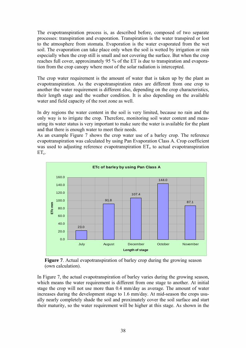
The evapotranspiration process is, as described before, composed of two separate processes: transpiration and evaporation. Transpiration is the water transpired or lost to the atmosphere from stomata. Evaporation is the water evaporated from the wet soil. The evaporation can take place only when the soil is wetted by irrigation or rain especially when the crop still is small and not covering the surface. But when the crop reaches full cover, approximately 95 % of the ET is due to transpiration and evapora-tion from the crop canopy where most of the solar radiation is intercepted. The crop water requirement is the amount of water that is taken up by the plant as evapotranspiration. As the evapotranspiration rates are different from one crop to another the water requirement is different also, depending on the crop characteristics, their length stage and the weather condition. It is also depending on the available water and field capacity of the root zone as well. In dry regions the water content in the soil is very limited, because no rain and the only way is to irrigate the crop. Therefore, monitoring soil water content and meas-uring its water status is very important to make sure the water is available for the plant and that there is enough water to meet their needs. As an example Figure 7 shows the crop water use of a barley crop. The reference evapotranspiration was calculated by using Pan Evaporation Class A. Crop coefficient was used to adjusting reference evapotranspiration ETo to actual evapotranspiration ETc.

ETc of barley by using Pan Class A

23.0

91.8

107.4

144.0

87.1

0.0

20.0

40.0

60.0

80.0

100.0

120.0

140.0

160.0

July August December October November

Length of stage

ETc

mm

Figure 7. Actual evapotranspiration of barley crop during the growing season (own calculation).

In Figure 7, the actual evapotranspiration of barley varies during the growing season, which means the water requirement is different from one stage to another. At initial stage the crop will not use more than 0.4 mm/day as average. The amount of water increases during the development stage to 1.6 mm/day. At mid-season the crops usu-ally nearly completely shade the soil and proximately cover the soil surface and start their maturity, so the water requirement will be higher at this stage. As shown in the

38

Figure 7 it is about 4.0 mm/day. At the end-season the water use decreased to be 3.5 mm/day. 19 Irrigation scheduling of a barley crop by using water budget method Water budget method is considering soil water storage reservoir as a bank. This reser-voir can hold a limited amount of water that is available for crops. At the same time, adding too much water to this soil reservoir will cause loss of water as deep percola-tion. When the crop evapotranspiration or the crop water use has been calculated, it is pos-sible to estimate the status of the soil reservoir and irrigation time by using the water balance equation (Nyvall, 2004): (Equation 20)

CSWC = PSWC + EP + IRR – ETc – DP (20)

where CSWC = current soil water content (today) [mm] PSWC = previous soil water content (yesterday) [mm] EP = effective precipitation since yesterday [mm] IRR = irrigation since yesterday [mm] ETc = crop evapotranspiration [mm] DP = deep percolation, water lost beyond the root zone [mm]

Each parameter in this equation describes the important factors that are determining the irrigation of the crops in the field. The crop root zone can be visualized as a reser-voir where water is temporarily stored for use by the crop. Inputs to that reservoir occur from both rainfall and irrigation. Since rainfall is very limited in dry regions the inputs occur mainly from irrigation. If the capacity of the soil-water reservoir (the volume of water stored in the crop root zone) and the daily rates of ET extraction from that reservoir are known, the date of the next irrigation and the amount of water to be applied can be determined. Thus, ET and soil-water storage capacity in the plant root zone is the basic information needed to use the water budget method for irriga-tion scheduling. The irrigation scheduling by water budget method consist of different steps as fol-lowing: - Determine soil water storage capacity, available soil moisture, maximum allow-

able deficit and the depth of root zone over the growing season. - Determine effective precipitation of rainfall by collected daily rainfall from cli-

mate station. In dry climate when rainfall is less than 5 mm, it does not add any moisture to the reservoir as most of it is evaporated before entering the soil, so in this case the effective rainfall is zero. If rainfall is over 5 mm, only 75 % of it will be considered as effective precipitation (Van der Gulik, 2004).

EP = (RAIN – 5) × 0.75 (21) where EP= effective rainfall [mm] and RAIN = rainfall [mm]

- Determine the net depth of irrigation water applied, which is the application rate and the length of the irrigation time. This step can be done when irrigation occurs.

39

- Determine daily crop evapotranspiration rates as explained in the calculation part of evapotranspiration above.

- Calculate water balance by start to obtain the current soil water storage (CSWC) by adding effective precipitation (EP) and net depth irrigation (IRR) to the previ-ous soil water storage (PSWC) and subtracting actual evapotranspiration ETc from it.

The next example shows daily water budget method of a barley crop. The crop starts growing the first of July and grows until the 27th of November in 2005. The location of this example is South Australia and the data to calculate evapotranspiration of the crop were obtained from Renmark Station. The total amount of rainfall was about 265 mm/year. Type of the soil was sandy loam which has soil water storage 125 mm m-1. The allowable soil water deficit of the barley was 50 %. The soil water storage was determined depending on the root depth. At initial stage the root depth was assumed to be 0.45 m. At development and mid-season the root depth was assumed to be 1.05 m and the late season 1.2 m. So related to the root depth the soil water storage each stage can be calculated as shown below: - At initial stage the soil water storage SWS

= root depth (m) × available soil water capacity (mm) = 0.45 m × 125mm = 56.25 mm

The allowable soil water deficit, AD = 50 % So the maximum soil water deficit = 56.25 × 50 % = 28.13 mm Therefore, during the initial stage which is 15 days the soil water storage should not exceed 56.25 mm as total storage at 0.45 m depth and the maximum deficit not ex-ceed 50 % which is 28.13 mm.

- At development and mid-season the crop growing and the root depth increase to about 1.05 m. Therefore:

The soil water storage = 1.05 × 125 mm = 131 The maximum soil water deficit = 131.25 mm × 50% = 65.7 mm.

- At the end season the crop become mature and its roots become bigger than the

other stages, related to that the soil water storage most be increased as well to about 1.20 m. So The soil water storage = 1.20 m × 125 mm = 150 mm The maximum soil water deficit = 150 mm × 50% = 75 mm

During each stage the soil water storage, SWS, must be adjusted related to the root depth and the maximum soil water deficit should not exceed 50 % from the total soil water storage at each stage. Therefore, when 50 % of 56.25 mm from the soil water storage at initial stage has been depleted from the soil, a total of 28.13 mm can be added by irrigation system and similar with the other stages.

40

Since actual evapotranspiration ETc of the barley was calculated daily the crop water requirement during the growing season is known. The rainfall must also be considered to calculate effective rainfall. Even if it is very limited, some time maybe we have high rainfalls which can be stored in the soil. After having considered all information that is needed for water budget method, we can calculate water budget for the whole season. It is important to start the water budget calculation after a thorough irrigation that fills the entire root zone. Then we can start with full soil water storage. Table 11 shows the calculation of irrigation scheduling of barley by using water budget method. Table 11. Example of irrigation scheduling calculation of barley crop by using water budget method (own calculation)

Date Previous soil water

storage PSWS +

Effective precipita-

tion EP +

Net Irriga-tion IRR -

Crop water use ETc =

Current soil water

storage CSWS

Initial stage * 2005-07-01 56.25 0 0 0.4 55.85

2005-07-02 55.85 0 0 0.6 55.25 2005-07-03 55.25 0 0 0.4 54.85 2005-07-04 54.85 0 0 0.3 54.55 Development stage ** 2005-07-16 54.2 0 77.05 0.6 130.65 2005-07-17 130.65 0 0 0.7 129.95 2005-07-18 129.95 0 0 0.4 129.55 2005-07-19 129.55 0 0 0.4 129.15

* At initial stage which is 15 day, we assumed the root depth 0.45 m and related to the soil water capacity of sandy loam which is 125 mm/m. The soil water storage at 0.45 m depth should be 56.25 mm. During the initial stage we must subtract daily crop water use from previous water soil storage PSWS. And we must irrigate when 50% of previous soil water storage has been depleted, which is 28.12mm.

** At development stage (30 day) the root depth increases to 1.05m and soil water storage must be increased to 131.25 mm. when the development stage start at 16th of July, the previous soil water storage was 54.2mm per root depth at initial stage which is 0.45m. Therefore we have to add 77.05mm by irrigation to adjust the previous soil water storage to 131.25 mm. during the development stage we subtract daily crop water use from previous soil water storage, as we said we must irrigate when almost 50% of previous soil water storage has been depleted. At mid season which is 65 day, we assumed the soil water storage is 131.25 mm and like we did at the initial and development stage daily crop water use is subtracted and we must irrigate when 50% of the previous soil water storage has been depleted. The same with the end stage, but we assumed the root depth almost 1 m. therefore the previous soil water storage is 125mm. Effective rainfall was considered during 8 days during the whole season.

The irrigation scheduling using the water budget method is based on estimation and should therefore be checked with soil moisture periodically. It is also important to monitor soil water content in the field and compare the calculated soil water content

41

to the actual measured water use once a week or every second week, and correct the calculated water balance when necessary (Van der Gulik, 2004). In Figure 8 the irrigation scheduling of barley during the growing season by using water budget method is illustrated.

Irrgation Scheduling of The Barley by Using Water Budget Method

0

20

40

60

80

100

120

140

1 10 19 28 37 46 55 64 73 82 91 100 109 118 127 136 145

Growing Length

Previous Soil WaterStorage PSWS

Effective Precipitation EP

Net Irrigation IRR

Crop Water Use Etc

Current Soil WaterStorage CSWS

Figure 8. Irrigation scheduling of barley crop by water budget method (own calculation).

From Figure 8 we can see that the crop was irrigated 7 times during the whole season. The crop was irrigated when 50 % of soil water storage is depleted. The effective pre-cipitation was considered by adding the effective amount of rainfall to the soil stor-age. 20 Effect of irrigation systems on irrigation scheduling efficiency The irrigation scheduling is good technology to decide how much water and when should we irrigate, but this method does not have high efficiency without considering the type of irrigation system. The efficiency of the irrigation scheduling is increasing by choosing the right irrigation system. As an example of how irrigation system has affected the crop yield, Komilov et al (2003) showed that drip irrigation system has increased the yield of cotton by 0.65 t ha-1 compared with surface irrigation. That means the water use efficiency was higher for drip irrigation than for furrow irriga-tion. 21 Choosing irrigation method To choose irrigation method, we must know the advantage and disadvantage of the various methods and which method suits the local conditions best. Unfortunately, in

42

many cases there is no single best solution: all methods have their advantages and dis-advantages (Brouwer et al., 1988). 21.1 Surface, sprinkler or drip irrigation The suitability of the various irrigation methods, i.e. surface, sprinkler or drip irriga-tion depends mainly on the following factors:

• Natural conditions: like soil type, slope, climate, water availability, water quality.

• Type of crop: surface irrigation can be used for all types of crops. Sprinkler and drip irrigation have high capital investment per hectare and are suitable for high value cash crops, such as vegetables and fruit trees. Drip irrigation is suited for irrigating individual plants or trees.

• Type of technology: the type of technology affects the choice of irrigation methods. In general, drip and sprinkler irrigation are technically more compli-cated methods compared to the surface irrigation.

• Previous experience with irrigation: the choice of irrigation method also depends on the irrigation tradition within the region or the country. Often it will be easier to improve the traditional irrigation method than to introduce a totally new method.

• Required labour inputs: surface irrigation requires a much high labour input - for construction, operation and maintenance- than sprinkler or drip irrigation. Surface irrigation requires accurate land levelling; regular maintenance and high level of farmers’ organization to operate the system compared to sprink-ler or drip irrigation.

• Costs and benefits: the estimation of cost of the irrigation method must in-clude cost of construction and installation and also the cost of operation and maintenance. These costs should be compared with the expected benefits.

• Which surface irrigation method is most suitable? There are some important factors that can help us to determine which surface irrigation method is suit-able (basin, furrow or border irrigation).

natural circumstances (slope, soil type) type of crop required depth of irrigation application level of technology previous experience with irrigation required labour inputs

21.2 Basin, furrow or border irrigation These techniques of irrigation are all defined as surface irrigation system. Each one has typical efficiency values which are presented in the Table 12. Table 12. Efficiency of different surface irrigation techniques (Keller, 1992) Surface irrigation technique Efficiency (%) Basin 70- 90 Border 70- 85 Furrow 65- 85

43

22 Forecasting schedules The forecast of water status is based on the forecasting of the evapotranspiration and rainfall. The length of time between irrigations will vary depending upon crop spe-cies, soil characteristics, location, time of year, temperature, and any particular micro environmental effects such as shade. Generally, if rain is forecasted in the next two days delay irrigation by forecast the climate data and crop coefficient. Generally the crop coefficient increases during the crop development stage, and then gradually decreases as the crop matures. It is difficult to include the rain in the irrigation scheduling, because sometimes the amount of rainfall is different from location to other location. The most common way of including rainfall in irrigation scheduling programs is to forecast the expected date of the next irrigation with different rainfall amounts (Heermann et al., 1990). In dry climate the amount of rainfall is very limited which often means that it can be neglected. Sometimes in some dry regions there is no rainfall at all during the grow-ing seasons. The measurement of rainfall is however very important in humid, semi humid or semiarid areas. There the rainfall might provide part of the water require-ments during the irrigation season (Phocaides, 2000). To increase the accuracy of the irrigation scheduling, rainfall should be measured for each scheduled field because the amounts may be highly variable. 23 Conclusions Irrigation scheduling is the key element to proper management of irrigation system by applying the correct amount of water at the right time to meet the requirement of water to the plants. Most crops will recover overnight from temporary wilting if less than 50 percent of the plant available water has been depleted. Therefore, the allowable depletion vol-ume generally recommended is maximum 50 percent. However, the recommended volume may range from 40 percent or less in sandy soils to more than 60 percent in clayey soils. The allowable depletion is also dependent on the type of crop, its stage of develop-ment, and its sensitivity to drought stress. For example, the allowable depletion recommended for some drought-sensitive crops (vegetable crops in particular) is only 20 percent during critical stages of development. On the other hand the allowable de-pletion may approach 70 percent during non-critical periods for drought-tolerant crops such as soybeans or cotton (Evans et al., 1996). When the irrigation scheduling is designed according to historical climate data or estimated by computer program, it is important to look at the crop in the field for colour change or measuring soil water status to make sure that the estimation is right, because this kind of scheduling does not take into account weather extremes which are different from year to year.

44

Irrigation scheduling technology is more readily accepted and implemented by irrigators with the use of automatic monitoring and prediction capacities (Heermann et al., 1990). The irrigation scheduling is more efficient when considering the irrigation method. By selected the right irrigation system we can control the flow rate and the distribution of the water in the field. 24 References Alam, M. & Rogers, D. H. 2001. Scheduling irrigation by electrical resistance blocks.

Kansas State University Agricultural Experiment Station and Cooperative Exten-sion Service. L-901 (Revised). [Online]. Available from: http://www.oznet.ksu.edu/library/ageng2/l901.pdf. [4 March 2007].

Allen, R. G., Pereira, L. S., Raes, D. & Smith, M. 1998. Crop evapotranspiration -Guidelines for computing crop water requirements. Rome: FAO. 300 pp. [Online] Available from: http://www.fao.org/docrep/X0490E/x0490e00.htm. [3 March 2007].

Azhar, A. H., Murty, V. V. N. & Phien, H. N. (1992) Modeling irrigation schedules of lowland rice with stochastic rainfall. Journal of Irrigation and Drainage Engi-neering. ASCE. Vol, 188(1) 36-55.

Broner, I. 2005. Irrigation Scheduling: The water balance approach. Colorado State University CSU, Cooperative Extension – Agriculture. No, 4,707. [Online] Avail-able from: http://www.ext.colostate.edu/pubs/crops/04707.html. [4 March 2007].

Brouwer, C., Prins, K., Kay, M. & Heibloem, M. 1988. Irrigation water management: Irrigation Methods. FAO. Irrigation water management, Training manual 5. [Online] Available from: http://www.fao.org/docrep/S8684E/S8684E00.htm. [5 March 2007].

Brouwer, C & Heibloem, M. 1986. Irrigation water management: Irrigation water needs. Food and Agriculture Organization of the United Nations. FAO. Irrigation water management, Training manual 3. Available from: http://www.fao.org/docrep/S2022E/S2022E00.htm. [5 March 2007].

Dalton, F. N., Herkelrath, W. N., Rawlins, D. S. & Rhodes, J. D. 1984. Time-domain reflectometry: Simultaneous measurement of soil water content and electrical conductivity with a single probe. Science. Vol 224(4652) 989-990.

Dregne, H. E. 1976. Soils of arid regions. Developments in Soil Science, 6. Elsevier Sci. Pub. Co. Amsterdam.

Edward, C. & Martin, P. 2001. Methods of determining when to irrigate. The Univer-sity of Arizona. College of Agriculture & Life Sciences,. Cooperative Extension. [Online]. Available from: http://cals.arizona.edu/pubs/water/az1220/. [4 March 2007].

Evans, R., Cassel, D. K. & Sneed, R. E. 1996. Soil, water, and crop characteristics important to irrigation scheduling. North Carolina Cooperative Extension Service. AG 452-1. [Online]. Available from: http://www.bae.ncsu.edu/programs/extension/evans/ag452-1.html. [7 March 2007].

45

Evett, S. R. 1994. TDR-Temperature arrays for analysis of field soil thermal proper-ties. In: Proceedings of the Symposium on Time Domain Reflectome-try in Environmental, Infrastructure and Mining Applications, Sept. 7-9, 1994. Northwestern University, Evanston, Illinois. USDA. of Interior, Bureau of Mines, Special Publication SP 19-94. [Online]. Available from: http://www.cprl.ars.usda.gov/Soil%20Water%20Papers_Presentations/tdrsym.pdf [31 March 2007]

Evett, S. R. & Steiner, J. L. 1995. Precision of neutron scattering and capacitance type soil water content gauges from field calibration. Soil Science Society of America Journal, 59(4).961-968. [Online]. Available from: http://www.cprl.ars.usda.gov/Soil%20Water%20Papers_Presentations/NP_CAP.PDF. [31 March 2007].

FAO. 1996. Irrigation scheduling: From theory to practice –Proceedings. Food and Agriculture Organization of United Nations. ICID-CIID. Water Reports 8. Rome. ISBN 92-5-103968-2. [Online]. Available from: http://www.fao.org/docrep/W4367E/W4367E00.htm#Contents. [31 March 2007].

FAO. 2003. Cropwat. Land and Water development division. http://www.fao.org/landandwater/aglw/cropwat.stm

Hatfield, J. I. 1990. Methods of estimating evapotranspiration. In: Stewart, B. A., & Nielsen, D. R. (editors) Irrigation of Agricultural Crops: Agronomy 30. American Society of Agronomy. Madison.

Heermann, D. F. 1985. ET in irrigation management. In Proceedings of the National Conference on Advances in Evapotranspiration. ASAE Publication 14-85. p 323-334.

Heermann, D. F., Martin, D. L., Jackson, R. D., & Stegman, E. C. 1990. Irrigation scheduling controls and techniques. In: Stewart, B. A., & Nielsen, D. R (editors) Irrigation of Agricultural Crops. Agronomy 30. American Society of Agronomy. Madison.

Heimovaara, T. J. & Bouten, W. (1990) A computer-controlled 36-channel time do-main reflectometry system for monitoring soil water contents. Water Resources Research. Vol 26(10)2311-2316

Hoffman, G. J., Howell, T. A. & Solomon, K. H., 1990. Management of farm irriga-tion system. American Society of Agriculture Engineers. St. Joseph, Mi. (USA). ISBN 0-929355-11, ISSN 3. p 1094.

Hillel, D. 1980. Fundamentals of soil physics. Academic Press, New York. 385p. ISBN-13: 978-0-12-348560-1.

Hillel, D. 1990. Role of irrigation in agricultural systems. In: Stewart, B. A., & Niel-sen, D. R. (editors) Irrigation of Agricultural Crops: Agronomy 30. American So-ciety of Agronomy. Madison

Idso, S. B., Reginato, R. J. & Farah, S. M. 1982. Soil and atmosphere-induced plant water stress in cotton as inferred from foliage temperature. Water Resources Re-search. Vol 18, No 4, 1143-1148. ISSN 0043-1397.

Irmak, S. & Haman, D. Z.. 2003. Evapotranspiration: potential or reference. Univer-sity of Florida, IFAS Extension. ABE 343. [Online]. Available from: http://edis.ifas.ufl.edu/AE256. [7 March 2007].

46

Jackson, R. D., Idso, S. B., Reginato, R. J. & Pinter, P. J. 1981. Canopy temperature as a crop water stress indicator. Water Resource Research. Vol 17. No 4. 1133-1138.

Jackson, R. D. 1982. Canopy temperature and crop water stress. Advance in irrigation volume 1, Academic Press, New York. p 43-85.

Jensen, M. E., Burman, R. D. & Allen, R. G (editors). 1990a. Evapotranspiration and irrigation water requirements. ASCE Manuals and Reports on Engineering Prac-tice, No. 70. ISBN-10: 0872627632. ISBN-13: 9780872627635.

Jensen, M. E., Rangeley, W. R., & Dieleman, P. J. 1990b. Irrigation trends in world agriculture. In: Stewart, B. A & Nielsen, D. R (editors) Irrigation of Agriculture Crops. Agronomy 30. American Society of Agronomy. Madison.

Keller, J. 1992. Irrigation scheme design for sustainability. Advances in planning, de-sign and management of irrigation systems as related to sustainable land use. Leu-ven, Belgium. pp 217-234.

Komilov, B., Ibragimov, N., Esanbekov, Y., Evett, S. & Lee, H. 2003. Irrigation scheduling study of drip irrigated cotton by use of soil moisture neutron probe. Proceedings of the national workshop “Developing cotton and winter wheat agro-technologies, 24-25 December 2002, UNCGRI, Tashkent ,Uzbekistan. [Online]. Available from: http://www.cprl.ars.usda.gov/wmru/pdfs/PaperDripIrrigatedCotton2002-3_as_published.pdf. [7 March 2007].

Muñoz-Carpena, R. 2004. Field devices for monitoring soil water content. University of Florida. Institute of Food and Agricultural Sciences.. Bulletin 343. [Online]. Available from: http://edis.ifas.ufl.edu/AE266. [7 March 2007].

Nyvall, J. 2004. Sprinkler irrigation scheduling using a water budget method. British Columbia Ministry of Agriculture, Food and Fisheries. Water Conservation Fact-sheet.. [Online]. Available from: http://www.agf.gov.bc.ca/resmgmt/publist/500series/577100-3.pdf [7 March 2007].

Penman H L (1948) Natural evaporation from open water, bare soil and grass. Pro-ceedings. Royal Society, London, United Kingdom. Series A193 120-146.

Penman H L (1963) Vegetation and hydrology. Technical Communication No. 53. Commonwealth Bureau of Soils, Harpenden, United Kingdom.

Pereira, L. 1996. Surface irrigation systems. In: Sustainability of irrigated agriculture. L.S. Pereira, R.A. Feldes, J.R. Gilley and B. Lesaffre (eds.). NATO ASI Series, Kluwer Academic Publishers, Dordrecht. Vol 312. p 269-290. ISSN 0304-9930.

Phocaides, A. 2000. Technical Handbook on Pressurized Irrigation techniques. Food and Agriculture Organization of the United Nations. Rome. [Online]. Available from: ftp://ftp.fao.org/agl/aglw/docs/pressirrig.pdf. [8 March 2007].

PIRSA.(2007). Weather data for IRES v2 users. Department of Primary Industries and Resources, South Australia [Online] Available from http://www.pir.sa.gov.au/pages/agriculture/horticulture/iresweather.htm:sectID=643&tem pID=1 [24 May 2007]

Ramadan, K. 1995. Libyan soils. Department of soil sciences, Alfath University. Na-tionality Organization of Science Research.

47

Schwab, G. O., Fangmeier, D. D. & Elliot, W. J. 1995. Soil and water management systems. Publisher Wiley, J., and Inc, S. ISBN-10: 0471109738. p 255-272.

Shih, S. F., Allen, L. H., Jr., Hammond, L. C., Jones, J. W. & Rogers, J. S. 1983. Ba-sin wide water requirement estimation in southern Florida. Transactions of the ASAE. Vol 26. No 3. p 760-766.

Shock, C. 2006. Efficient irrigation scheduling. Oregon State University, Malheur Agricultural Experiment Station. Information for Sustainable Agriculture. [Online]. Available from: http://www.cropinfo.net/irrigschedule.htm. [7 March 2007].

Tam, S. 2006. Irrigation scheduling with tensiometers. Ministry of Agriculture and Lands. Water Conservation Factsheet. [Online]. Available from: http://www.al.gov.bc.ca/resmgmt/publist/500series/577100-2.pdf. [8 March 2007].

Tan, C. S. 1990. Irrigation scheduling for tomatoes - water budget approach. Ministry of Agriculture Food and Rural Affairs. Factsheet. [Online]. Available from: http://www.omafra.gov.on.ca/english/crops/facts/90-049.htm. [7 March 2007].

Tan, C. S. & Layne, R. E. C. 1990. Irrigation scheduling for fruit crops. Ministry of Agriculture Food and Rural Affairs. Factsheet [Online]. Available from: http://www.omafra.gov.on.ca/english/crops/facts/90-069.htm. [7 March 2007].

Tron, G., Peyremorte, P. & Berthomé, P. 1988. Développement des moyens pour améliorer la conduite des irrigations de surface: Conduite des arrosages en systèmes gravitaires modernisés. Etud. RNED-HA, SCP, Cemagref, 121 p.

Van der Gulik, T. & Nyvall, J. 2001. Crop coefficients for use in irrigation Schedul-ing. British Columbia, Ministry of Agriculture, Food and Fisheries. Water Con-servation Factsheet. [Online]. Available from: http://www.agf.gov.bc.ca/resmgmt/publist/500series/577100-5.pdf. [7 March 2007].

Van der Gulik, T. 2004. Trickle irrigation scheduling using evapotranspiration data. British Columbia, Ministry of Agriculture, Food and Fisheries.. Water Coservaton Factsheet. [Online]. Available from: http://www.agf.gov.bc.ca/resmgmt/publist/500series/577100-4.pdf. [7 March 2007].

Van der Gulik, T. 2006. Irrigation scheduling techniques. British Columbia, Ministry of Agriculture and Lands. Water Conservation Factsheet.. [Online]. Available from: http://www.agf.gov.bc.ca/resmgmt/publist/500series/577100-1.pdf. [7 March 2007].

Wallace, J. S. 2000. Increasing agricultural water use efficiency to meet future food production. Agriculture Ecosystems & Environment.82, 105-119. [Online]. Avail-able from: http://www.cse.polyu.edu.hk/~cekslam/Paper/science28.pdf. [7 March 2007].

Waskom, R. M. 1994. Best management practices for irrigation management. Colo-rado State, University Cooperative Extension. Bulletin #XCM-173. [Online]. Available from: http://www.ext.colostate.edu/Pubs/crops/xcm173.pdf. [7 March 2007].

Whitfield, D. M., Wright,G. C., Gyles, O. A. & Taylor, A. J. 1986. Growth of Lu-cerne (Medicago sativa L.) in response to frequency of irrigation and gypsum ap-

48

plication on heavy clay soil. Irrigation Science. 7, 37-52. [Online] Available from: http://www.springerlink.com/content/w4xgg58372302365/fulltext.pdf. [22 March 2007]

Wraith, J. M. & Or, D. 1999. Temperature effects on soil bulk dielectric permittivity measured by time domain reflectometry: Experiment. Water Resources Research. Vol 35. I ssue 2. p 371- 384.

49