WORKING PAPER 6/2006

Is Economic Growth Sustainable? Environmental Quality of Indian States Post

1991

Sacchidananda Mukherjee Research Scholar

and

Vinish Kathuria

Associate Professor

MADRAS SCHOOL OF ECONOMICS Gandhi Mandapam Road

Chennai 600 025 India

March 2006

Is Economic Growth Sustainable? Environmental Quality Of Indian States Post 1991

Sacchidananda Mukherjee*

Research Scholar

and

Vinish Kathuria Associate Professor

.

_____________________ * Corresponding author Tel.: +91-44-2235 2157; 2230 0304; 2230 0307; Cell: +91 9840699343 Fax: +91-44-2235 2155; 2235 4847 E-mail address: sachs.mse@gmail.com

WORKING PAPER 6/2006 March 2006 Price : Rs.35

MADRAS SCHOOL OF ECONOMICS Gandhi Mandapam Road Chennai 600 025 India Phone: 2230 0304/ 2230 0307/2235 2157 Fax : 2235 4847 /2235 2155 Email : info@mse.ac.in Website: www.mse.ac.in

IS ECONOMIC GROWTH SUSTAINABLE? ENVIRONMENTAL QUALITY OF INDIAN STATES POST 1991

Sacchidananda Mukherjee* and

Vinish Kathuria

Abstract This study is an attempt to investigate the relationship between environmental quality and per capita NSDP (i.e., Environment Kuznets Curve, EKC) of 14 major Indian States in the light of their very high economic growth in the post-liberalisation period. The analysis involves first ranking the States on the basis of their environmental quality, and then checking the relationship. The analysis captures both temporal and spatial aspects of environmental quality by ranking the States in two time periods – (i) early 1990s (1990 - 1996) and (ii) late 1990s (1997 - 2001). The results indicate that the relationship between environmental quality and per capita NSDP is slanting S-shaped. Except Bihar all other States are on the upward sloping curve of the EKC. The results suggest that the economic growth is mostly at the cost of environmental quality. ________________

* Acknowledgement

We are grateful to Prof. Paul P. Appasamy, for his encouragement to take up this study. Our discussions with Prof. U. Sankar and Prof. Ramprasad Sengupta led to a substantial improvement in this paper. Earlier version of the paper has been presented at the International Conference on ‘Environment and Development: Developing Countries Perspective’ held in Jawaharlal Nehru University, New Delhi, April 7-8, 2005. We wish to thank the conference participants for their useful comments and observations. The usual disclaimers nevertheless apply.

1. Introduction

The nineties have been watershed in the economic history of India,

as the country embarked on liberalisation process in 1991. The liberalisation

not only induced various States to enhance their production capacities but

also facilitated restructuring of their economic activities. However, inter-State

disparities in natural resources endowments have played a crucial role in this

restructuring. Based on inter- and intra-sectoral differences in economic

activities, different States have put different level of stress on their natural

resources. The liberalisation process and emphasis to grow faster has

resulted in on an average nearly 7-8 per cent growth rates of different States

in the 1990s against 3-4 per cent average growth during the 1980s.1

However, in their pursuit to grow rapidly, most of the Indian States seem to

have neglected key environmental and natural resources concerns, which in

turn has resulted in large-scale depletion of natural resources and rapid

degradation of the environment (see for example, Nadkarni, 2000; Kothari,

1996 among others for evidence).

For a country, having high dependence on natural resources,

managing and protecting the environment is the key to ensure

environmental and economic sustainability. In fact, this is also one of the

Millennium Development Goals (MDGs) of the United Nations.2

Economic growth plays a crucial role for socio-economic

development. However, economic development and environmental

sustainability are not supplementary to each other. Sustained development is

elusive without sustainable environment, especially for developing countries

1 Source: EPWRF (2003). See Table 7 of the paper for State-wise growth rate during the 1990s. 2 It is to be noted that among 18 Targets of the MDGs, six (Targets 2, 5, 8, 9 and 10) are directly linked to sustainability and sustainable development issues (see http://www.developmentgoals.org/ for these goals).

2

like India, Kenya where a large section of the society depends on natural

resources for livelihood, directly or indirectly (Dasgupta, 2001). Unlike

developed countries, developing countries do not have adequate financial

resources to tackle the problem of natural resource depletion or degradation.

Hence it is imperative that developing countries should protect their natural

resources, rather than searching for solutions after depletion and

degradation. The natural resource degradation, if not checked, will result in

large-scale poverty and destitution, and can hamper the very process of

socio-economic development of the populace (Agarwal, 1995 and Nadkarni,

2000).

Under this backdrop, the main objective of this study is to see - how

the States have performed after economic liberalisation with respect to the

protection of environmental quality? To investigate the issue, the study first

captures inter-State variations in the environmental situations by ranking the

States according to their environmental quality. Once the environmental

status of different States is found, the study then tests whether economic

development has any relationship with environmental quality or not?

The analysis is based on various secondary environmental

information available for 14 major Indian States for the time period 1990 to

2001. In order to fathom the change in environmental quality due to

liberalisation process, the period is bifurcated into two sub-periods - early

1990s (1990-1996) and late 1990s (1997-2001). For both the sub-periods,

63 environmental indicators have been clustered under 8 broad

environmental groups. To rank the States under each group Principal

Component Analysis (PCA) method of factor analysis has been used. The

ranks obtained by an individual State across the different environmental

criteria are then added using Borda Rule to get the final environmental

3

quality (EQ) score. Finally, we compare the EQ scores of the States with their

per capita Net State Domestic Product (PCNSDP) to verify the Environmental

Kuznets Curve (EKC)3 hypothesis using a multivariate regression analysis.

The analysis shows that for early 1990s, the better performing

States with respect to environmental quality are Andhra Pradesh (AP),

Orissa, Kerala and West Bengal (WB), and for the late 1990s are Madhya

Pradesh (MP), Orissa, Bihar and Uttar Pradesh (UP). For both the sub-

periods, Haryana, Punjab, Gujarat, Karnataka are some of the poor

performing States in terms of environmental quality. During the late 1990s,

MP, Maharashtra, Bihar and UP have improved their rankings, whereas AP,

WB and Tamilnadu (TN) have lost their earlier positions.

The relationship between economic development, measured by the

PCNSDP at constant (1993-94) prices, and the EQ score shows non-linearity

as predicted in EKC. Some of the States having low PCNSDP have better

environmental quality, however other States like Maharashtra, Gujarat, TN,

WB and Karnataka are on the upward sloping curve of the EKC and may

continue to degrade environment if continue to grow at the same pace.

The remaining paper is organised as follows: Section 2 gives a brief

literature review of environmental ranking at country level, followed by

studies carried out to test Environmental Kuznets Curve (EKC) hypothesis.

Section 3 gives methodology, data sources and description of the variables.

Section 4 provides the results and analysis of environmental quality of

different States, whereas Section 5 gives the results for EKC hypothesis.

Paper concludes with Section 6.

3 Environmental Kuznets Curve (EKC) originates from the works of Simon Kuznets. The original Kuznets curve show how income inequality changes as income in a country rises, wherever EKC shows how environmental quality change with change in income in a country.

4

2. Literature Review

2.1 Environmental Sustainability Index - A Review

As a scientific tool to measure environmental performance across the

geographical area, ranking on the basis of construction of environmental

index has always been an important area of research both for individual

researchers (see for example, Rogers et al., 1997; Adriaanse et al., 1995;

Adriaanse, 1993 among others) and various development agencies (WWF,

2002; CBD/UNEP, undated; The Fraser Institute by Jones et al., 2002;

RIVM/UNEP, undated).

Most of these studies, especially by the multilateral agencies,

compute the index on yearly basis, which has significant developmental and

environmental policy implications. However these studies differ considerably

in their scope, coverage area, methodology and in the selection of variables

for the construction of an index.4

The most recent index of environmental sustainability has been

constructed by Esty et al. (2005) for 146 countries. The main objective of the

study is to provide a composite profile of national environmental stewardship

in the protection of environment over the next several decades. It is based

on a compilation of 21 indicators that derive information from 76 underlying

data sets covering all aspects of environment.5

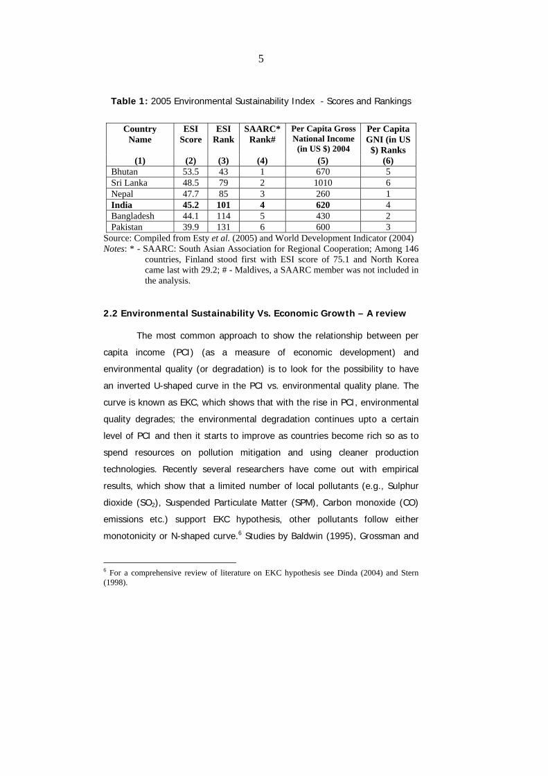
Table 1 gives the details of the scores and ranks obtained by the South Asian

countries in the 2005 Environmental Sustainability Index (ESI). It shows that

India’s position is 101st, whereas other South Asian countries like Bhutan, Sri

Lanka and Nepal are far ahead in terms of Environmental Sustainability. 4 For more details see http://farmweb.jrc.cec.eu.int/ci/Indexes.htm. 5 See Esty et al. (2005) for details about these indicators.

5

Table 1: 2005 Environmental Sustainability Index - Scores and Rankings

Country Name

ESI Score

ESI Rank

SAARC* Rank#

Per Capita Gross National Income

(in US $) 2004

Per Capita GNI (in US

$) Ranks (1) (2) (3) (4) (5) (6)

Bhutan 53.5 43 1 670 5 Sri Lanka 48.5 79 2 1010 6 Nepal 47.7 85 3 260 1 India 45.2 101 4 620 4 Bangladesh 44.1 114 5 430 2 Pakistan 39.9 131 6 600 3

Source: Compiled from Esty et al. (2005) and World Development Indicator (2004) Notes: * - SAARC: South Asian Association for Regional Cooperation; Among 146

countries, Finland stood first with ESI score of 75.1 and North Korea came last with 29.2; # - Maldives, a SAARC member was not included in the analysis.

2.2 Environmental Sustainability Vs. Economic Growth – A review

The most common approach to show the relationship between per

capita income (PCI) (as a measure of economic development) and

environmental quality (or degradation) is to look for the possibility to have

an inverted U-shaped curve in the PCI vs. environmental quality plane. The

curve is known as EKC, which shows that with the rise in PCI, environmental

quality degrades; the environmental degradation continues upto a certain

level of PCI and then it starts to improve as countries become rich so as to

spend resources on pollution mitigation and using cleaner production

technologies. Recently several researchers have come out with empirical

results, which show that a limited number of local pollutants (e.g., Sulphur

dioxide (SO2), Suspended Particulate Matter (SPM), Carbon monoxide (CO)

emissions etc.) support EKC hypothesis, other pollutants follow either

monotonicity or N-shaped curve.6 Studies by Baldwin (1995), Grossman and

6 For a comprehensive review of literature on EKC hypothesis see Dinda (2004) and Stern (1998).

6

Krueger (1995), Selden and Song (1994), Panayotou (1993), Shafiq and

Bandyopadhyay (1992) and Pezzey (1989) based on ambient concentration

of pollutants support EKC hypothesis. Similarly, studies conducted by Bruvoll

and Medin (2003); de Bruyn et al. (1998) and Carson et al. (1997),

considering the actual emission of pollutants instead of their ambient

concentration also support the EKC hypothesis.

However most of the studies on EKC have considered only a few

pollutants, and have come out with individual pollutant wise EKC. Choosing

few pollutants and verifying the EKC might not be true reflection of economic

activity and its polluting nature. This is because of two reasons - (a) the

economic activity, which generates that pollutant, may not have significant

impact on the economy to substantially influence the PCI or vice versa; and

(b) ambient concentration of pollutant is not only function of its actual

emission but also depends on several other factors which influence its

dispersion and assimilation.7 Therefore instead of single pollutant, if we take

a composite indicator of pollutants, it would show the actual environmental

quality. The only study that has looked into the environment quality as a

whole is by Jha and Bhanu Murthy (2001). The authors construct an

environmental degradation index (EDI) for 174 countries and compare that

with human development index (HDI) instead of PCI. The study finds inverse

link between EDI and HDI and do not find supporting evidence for inverted

U-shaped EKC. The study shows that an inverted N-shaped global EKC does

indeed exist.

The present study attempts to establish the EKC relationship

between per capita NSDP and environmental quality as a whole instead of

using only selected pollutants.

7 Refer Kathuria (2004, 2002) indicating the relevance of other factors in influencing ambient air quality.

7

3. Methodology, Data Sources and Descriptions of the Variables

3.1 Methodology

The depletion and degradation of natural resources and

environmental pollution is mainly an environmental management aspect,

whereas the endowments of natural resources (forests, land and water) are

mostly driven by the geographical location of the State and the prevailing

climatic and ecological situations. As a result, human activities have limited

impact on latter. However, the two effects (endowment effect and efficiency

in natural resource management effect) can be segregated by the change in

the natural resource position with reference to a base year. As for example,

comparing the forest resources (simply by taking the percentage of

geographical area under forests land) between Madhya Pradesh and

Rajasthan may show Madhya Pradesh standing apart from Rajasthan, but it

will be erroneous to conclude that forest conservation practices of Madhya

Pradesh are better as compared to Rajasthan. This is because Rajasthan is

endowed with very little forest resources. However, if we take the change in

the forest area (as a percentage of geographical area) during any two

periods and rank them, one can infer about their forest conservation

practices. This study considers the environmental management efficiency

effect, besides taking into consideration the size effect of the States.

3.2 Steps Involved

The analysis is carried out in three steps. In Step 1, after

normalisation of the indicators, Principal Component Analysis (PCA) method

of factor analysis is used to construct a composite indicator for an

environmental group.8 For each environmental group, the first factor score is

used to rank the States. The underlying assumption is that with all the

8 Each environmental group constitutes a large number of environmental indicators (refer Appendix 2) from which a composite indicator is derived.

8

indicators of a group taken together, the set determines situation of the

State with respect to that variable (environmental quality). In other words,

all the indicators of a variable when combined for a certain State should

reflect the environmental status of the State with respect to that particular

criterion. For example, the ambient condition of air pollution in a State is not

manifested by only SPM concentration, but by the concentration of all the

pollutants (SO2, Oxides of nitrogen (NOx), SPM) in both - residential and

industrial areas.

In Step 2, based on Borda rule,9 a broad environmental quality score

(EQSi) is constructed by adding the ranks obtained by each State with

respect to the individual environmental groups. If Eij is the rank of the ith

State with respect to jth environmental variable (group), then EQSi of the ith

State for 8 environmental groups is:

∑=

=8

1jiji EEQS

In Step 3, the States are ranked according to their EQSi, where

environmental quality rank (EQRANK) of the ith State is the rank of the State

with respect to EQSi over i=1 to 14.

In the second part of the paper, EKC hypothesis is tested by running

multivariate regression equation using EQS as dependent variable and log of

per capita income (LNPCI) as independent variable. Since the relation

between the two is inverted U-shape, the non-linearity is accounted for by

taking a square of the income term (LNPCI2). The literature suggests that

the pollution (or environmental quality) is affected not only by the income

but also by a number of other variables like share of agriculture in GDP or

what proportion of employment is dependent on primary sector or population

density or awareness etc. (see for example Aldy, 2004; Andreoni and

9 The Borda Rule or Borda rank is the rank order scoring rule for ordinal aggregation. The rule can also be viewed as voting rule, where under each environmental criterion (voter), the States are ranked (voted) from high to low EQ. The rule invariably yields a complete ranking of alternatives (see Dasgupta, 2001).

9

Levinson, 2001 and Grossman and Krueger, 1995 among others10). Thus,

following equation is estimated to establish the EKC hypothesis:

ititititit XLNPCILNPCIEQS εγββα ++++= 210 (1)

where, i=1 to 14 and t is the two time periods for which data is pooled and εi

is the error term and εi ~ N(0,1), iid; Xi captures all other explanatory

variables (e.g., share of agriculture in GSDP (AGR), workers in agricultural

sector (AGRWRK), rural literacy rate (LITRU), extent of urbanization (URB),

share of manufacturing (MFG)). The saddle point of the EKC is obtained from

first order condition of equation 1.

⎟⎟⎟

⎠

⎞

⎜⎜⎜

⎝

⎛ −== Λ

ΛΛ

1

0

2exp)exp(*

β

βLNPCIPCI

3.3 Data and Variables

As indicated, the study considers 14 major Indian States – viz.,

Andhra Pradesh (AP), Bihar (BH), Gujarat (GUJ), Haryana (HR), Karnataka

(KAR), Kerala (KER), Madhya Pradesh (MP), Maharashtra (MH), Orissa (OR),

Punjab (PB), Rajasthan (RAJ), Tamilnadu (TN), Uttar Pradesh (UP) and West

Bengal (WB) – for which environmental information are available for the two

broad time periods – (a) early 1990s (1990-1996); and (b) late 1990s (1997-

2001). Since the data for various environmental indicators are available for

different time points, which are not necessarily falling within the time period

selected for our analysis, we have taken only those indicators which have at

10 It is to be noted that these relationships are easy to conceptualise, if one is trying to find relationship between a particular environment indicator (say CO2) and income. However, for a composite index, the relationship is difficult to predict. For example, increased urbanisation may lead to increased urban air pollution, but may also lead to fall in non-point source pollution, if the city is adequately covered with water and sanitation. In those circumstances, the relationship is more of exploratory.

10

least two observations, and one of these observations falling within the

boundary of our two time periods.

This analysis is mostly based on the State level secondary

information available in various published government reports and

databases. Appendix 1 gives the list of various sources used for the analysis.

The indicators have been normalised using appropriate measures of

size/scale of the States – geographical area, population and Gross State

Domestic Product (GSDP) at current prices. After an extensive literature

review and based on the data availability at the State level, for both the

periods 63 environmental status indicators are grouped under 8 broad

environmental variables as given in Table 2. Appendix 2 gives the

descriptions of the groups and different indicators used to form each group.

Table 2: Descriptions of the Environmental Groups

Groups Group Descriptions Number of Indicators

AIRPOL Air Pollution 6

INDOOR Indoor Air Pollution Potential 6

GHGS Green House Gases (GHGs) Emissions 4

ENERGY Pollution from Energy Generation and Consumption 12

FOREST Depletion and Degradation of Forest Resources 11

WATER Depletion and Degradation of Water Resources 10

NPSP Nonpoint Source Water Pollution Potential 7

LAND Pressure and Degradation of Land Resources 7

Total 63

11

3.4 Construction of Variables for EKC

As the second part of the paper involves verifying EKC, various

control variables have been used. The share of agriculture in GSDP (AGR)

has been computed as the average for the period 1993-94 to 1995-96 for

period 1 and average for 1997-98 to 1999-2000 for period 2. The average is

taken to smoothen out uneven fluctuations. AGRWRK is the agricultural

workers (including cultivators and agricultural labourers) as a percentage of

total workers. LITRU is the percentage of rural literate population (defined as

7 years and above). Apart from this, Urbanisation (URB), i.e., extent of

people living in urban areas and share of Manufacturing in GSDP (MFG) are

also included.

3.5 Estimation Issues

For factor analysis, Varimax (with Kaiser normalisation) method of

factor rotation11 is applied using SPSS Statistical Software (Version 9.05).

The Kaiser-Meyer-Olkin (KMO) measure12 of sampling adequacy criteria has

been used to select a set of indicators for the factor analysis. Test statistics

indicate that in most cases it is greater than 0.60 and Bartlett's test of

sphericity13 is also significant at 0.01 level in most cases.

To verify the EKC hypothesis, multivariate OLS regressions are

carried out with EQS as dependent variable and log PCNSDP, log PCNSDP2

and other controlling variables. The estimation is carried out by pooling the

data for both the periods with a dummy variable for period 2.

11 Factor analysis attempts to identify underlying variables/ factors, that explain the pattern of correlations within a set of observed variables. The need for PCA is because some of the variables in a group may be correlated; dropping them will result in loosing vital information. 12 KMO measure of sampling adequacy tests whether the partial correlations among variables are small or not. 13 Bartlett's test of sphericity tests whether the correlation matrix is an identity matrix, which would indicate that the factor model is inappropriate. The tests are significant at 0.01 level, thus indicating model appropriateness.

12

4. Results – Constructing Environmental Quality Scores

4.1 Environmental Ranking of States during early 1990s

Table 3 gives the EQ score and ranking of 14 major Indian states for

period 1. It shows that during the early 1990s, Orissa, AP, Kerala and WB

are the four better performing States with respect to environmental quality.

On the other hand, Haryana, Punjab, Gujarat and Maharashtra are the four

worst performing States. AP and Orissa have the highest EQ ranking, as both

the States have done well in almost all the aspects of EQ. Except in indoor

air pollution control, Haryana has done badly in almost all other criteria.

From the table it is evident that different States have different strengths and

weaknesses in managing various aspects of environmental quality. For

instance, in early 1990s Kerala has managed air and indoor air pollution well,

whereas WB has done well in water resource management and so on.

Table 3: Ranks obtained by States for different EQ Criteria – Early 1990s

Criteria AIRPOL INDOOR GHGS ENERGY FOREST WATER NPSP LAND EQ Score EQRANK

State (1) (2) (3) (4) (5) (6) (7) (8) (9) (10)

Andhra Pradesh 4 3 4 3 1 4 12 3 34 1 Bihar 10 13 1 1 11 5 6 6 53 6

Gujarat 12 11 8 12 8 8 9 12 80 12

Haryana 6 9 12 13 7 12 13 14 86 14 Karnataka 7 5 13 9 10 10 7 2 63 9

Kerala 1 1 14 7 6 6 4 5 44 3

Madhya Pradesh 14 6 2 6 14 3 2 10 57 7

Maharashtra 8 12 9 11 13 9 3 11 76 11

Orissa 2 7 5 4 12 2 1 1 34 1 Punjab 9 10 11 14 2 14 14 8 82 13

Rajasthan 11 4 10 10 9 11 5 13 73 10

Tamilnadu 3 2 6 8 5 13 10 4 51 5

Uttar Pradesh 13 8 3 5 3 7 11 7 57 7

West Bengal 5 14 7 2 4 1 8 9 50 4

Note: EQ Score is obtained using Borda Rule

13

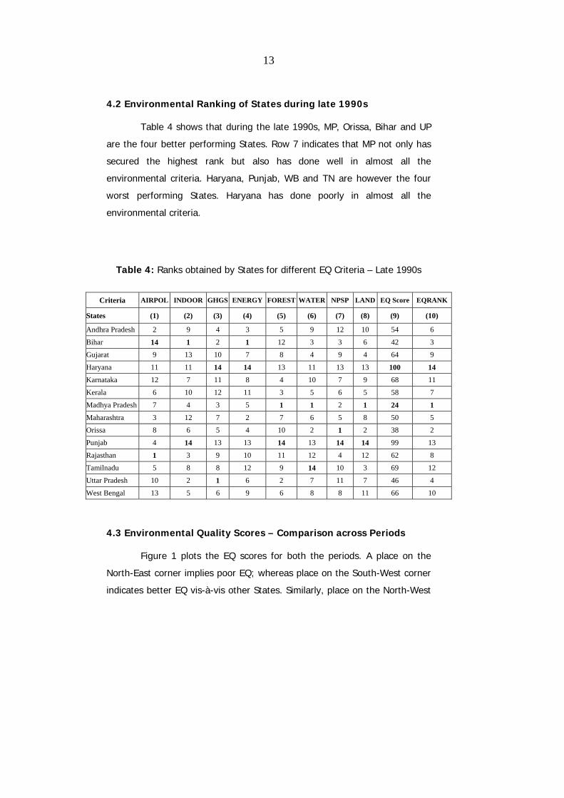
4.2 Environmental Ranking of States during late 1990s

Table 4 shows that during the late 1990s, MP, Orissa, Bihar and UP

are the four better performing States. Row 7 indicates that MP not only has

secured the highest rank but also has done well in almost all the

environmental criteria. Haryana, Punjab, WB and TN are however the four

worst performing States. Haryana has done poorly in almost all the

environmental criteria.

Table 4: Ranks obtained by States for different EQ Criteria – Late 1990s

Criteria AIRPOL INDOOR GHGS ENERGY FOREST WATER NPSP LAND EQ Score EQRANK

States (1) (2) (3) (4) (5) (6) (7) (8) (9) (10)

Andhra Pradesh 2 9 4 3 5 9 12 10 54 6

Bihar 14 1 2 1 12 3 3 6 42 3

Gujarat 9 13 10 7 8 4 9 4 64 9

Haryana 11 11 14 14 13 11 13 13 100 14 Karnataka 12 7 11 8 4 10 7 9 68 11

Kerala 6 10 12 11 3 5 6 5 58 7

Madhya Pradesh 7 4 3 5 1 1 2 1 24 1 Maharashtra 3 12 7 2 7 6 5 8 50 5

Orissa 8 6 5 4 10 2 1 2 38 2

Punjab 4 14 13 13 14 13 14 14 99 13

Rajasthan 1 3 9 10 11 12 4 12 62 8

Tamilnadu 5 8 8 12 9 14 10 3 69 12

Uttar Pradesh 10 2 1 6 2 7 11 7 46 4

West Bengal 13 5 6 9 6 8 8 11 66 10

4.3 Environmental Quality Scores – Comparison across Periods

Figure 1 plots the EQ scores for both the periods. A place on the

North-East corner implies poor EQ; whereas place on the South-West corner

indicates better EQ vis-à-vis other States. Similarly, place on the North-West

14

corner means EQ has degraded in the State and position on the South-East

corner means improvement in EQ over the period.

Figure 1: Environmental Quality Scores over Periods

Environmental Q uality (EQ ) Scores over Periods

HRPB

GUJ

MH

RAJ

KAR

UPBH

TNWB

KERAP

OR

MP

10

20

30

40

50

60

70

80

90

100

110

20 30 40 50 60 70 80 90 100EQ Score - Early 1990s

EQ S

core

- La

te 1

990s

The figure shows that Orissa has done well in both the periods with

respect to environmental quality. During late 1990s EQ Scores of AP, Kerala,

WB, and TN have gone up substantially, which implies that environmental

quality of these States has degraded during the period. For Punjab and

Haryana, the environmental quality has degraded further during late 1990s.

EQ Scores of MP, BH, UP, Rajasthan, Maharashtra and Gujarat has declined

as compared to the earlier scores. The environmental quality improvement

for MP is quite substantial, whereas for Karnataka, it has remained

unchanged. Based on the plot, it can be concluded that States like Haryana

and Punjab need special attention to check their environmental degradation.

15

5. Results – Testing for Environmental Kuznets Curve

5.1. Economic Development Vs. Environmental Quality

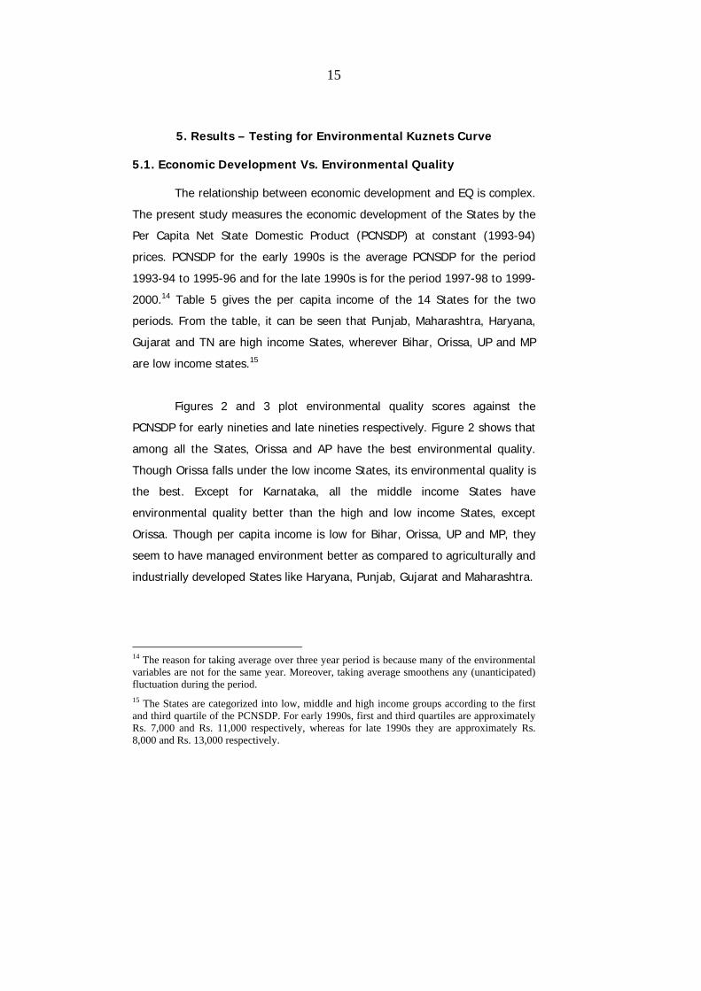
The relationship between economic development and EQ is complex.

The present study measures the economic development of the States by the

Per Capita Net State Domestic Product (PCNSDP) at constant (1993-94)

prices. PCNSDP for the early 1990s is the average PCNSDP for the period

1993-94 to 1995-96 and for the late 1990s is for the period 1997-98 to 1999-

2000.14 Table 5 gives the per capita income of the 14 States for the two

periods. From the table, it can be seen that Punjab, Maharashtra, Haryana,

Gujarat and TN are high income States, wherever Bihar, Orissa, UP and MP

are low income states.15

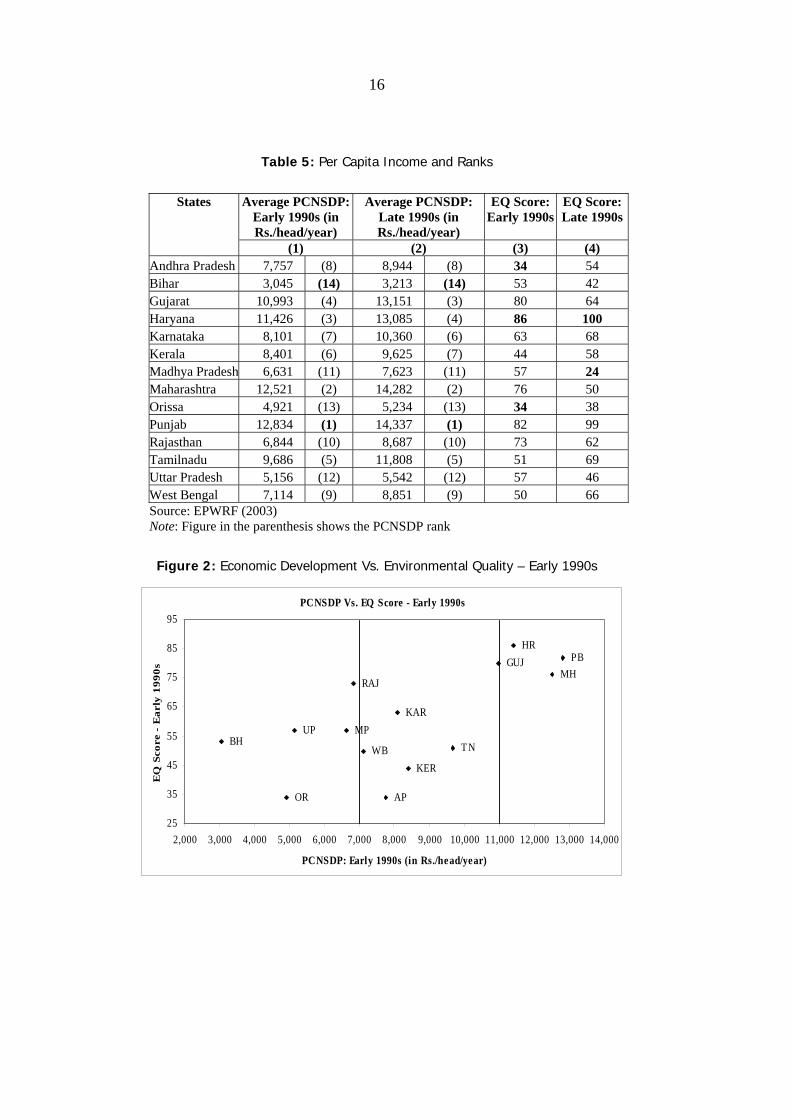
Figures 2 and 3 plot environmental quality scores against the

PCNSDP for early nineties and late nineties respectively. Figure 2 shows that

among all the States, Orissa and AP have the best environmental quality.

Though Orissa falls under the low income States, its environmental quality is

the best. Except for Karnataka, all the middle income States have

environmental quality better than the high and low income States, except

Orissa. Though per capita income is low for Bihar, Orissa, UP and MP, they

seem to have managed environment better as compared to agriculturally and

industrially developed States like Haryana, Punjab, Gujarat and Maharashtra.

14 The reason for taking average over three year period is because many of the environmental variables are not for the same year. Moreover, taking average smoothens any (unanticipated) fluctuation during the period. 15 The States are categorized into low, middle and high income groups according to the first and third quartile of the PCNSDP. For early 1990s, first and third quartiles are approximately Rs. 7,000 and Rs. 11,000 respectively, whereas for late 1990s they are approximately Rs. 8,000 and Rs. 13,000 respectively.

16

Table 5: Per Capita Income and Ranks

States Average PCNSDP: Early 1990s (in Rs./head/year)

Average PCNSDP: Late 1990s (in Rs./head/year)

EQ Score: Early 1990s

EQ Score: Late 1990s

(1) (2) (3) (4) Andhra Pradesh 7,757 (8) 8,944 (8) 34 54 Bihar 3,045 (14) 3,213 (14) 53 42 Gujarat 10,993 (4) 13,151 (3) 80 64 Haryana 11,426 (3) 13,085 (4) 86 100 Karnataka 8,101 (7) 10,360 (6) 63 68 Kerala 8,401 (6) 9,625 (7) 44 58 Madhya Pradesh 6,631 (11) 7,623 (11) 57 24 Maharashtra 12,521 (2) 14,282 (2) 76 50 Orissa 4,921 (13) 5,234 (13) 34 38 Punjab 12,834 (1) 14,337 (1) 82 99 Rajasthan 6,844 (10) 8,687 (10) 73 62 Tamilnadu 9,686 (5) 11,808 (5) 51 69 Uttar Pradesh 5,156 (12) 5,542 (12) 57 46 West Bengal 7,114 (9) 8,851 (9) 50 66 Source: EPWRF (2003) Note: Figure in the parenthesis shows the PCNSDP rank

Figure 2: Economic Development Vs. Environmental Quality – Early 1990s

PCNSDP Vs. EQ Score - Early 1990s

BH

OR AP

UP MP

WBKER

TN

KAR

RAJ

GUJHR

MHPB

25

35

45

55

65

75

85

95

2,000 3,000 4,000 5,000 6,000 7,000 8,000 9,000 10,000 11,000 12,000 13,000 14,000

PCNSDP: Early 1990s (in Rs./head/year)

EQ

Sco

re -

Ear

ly 1

990s

17

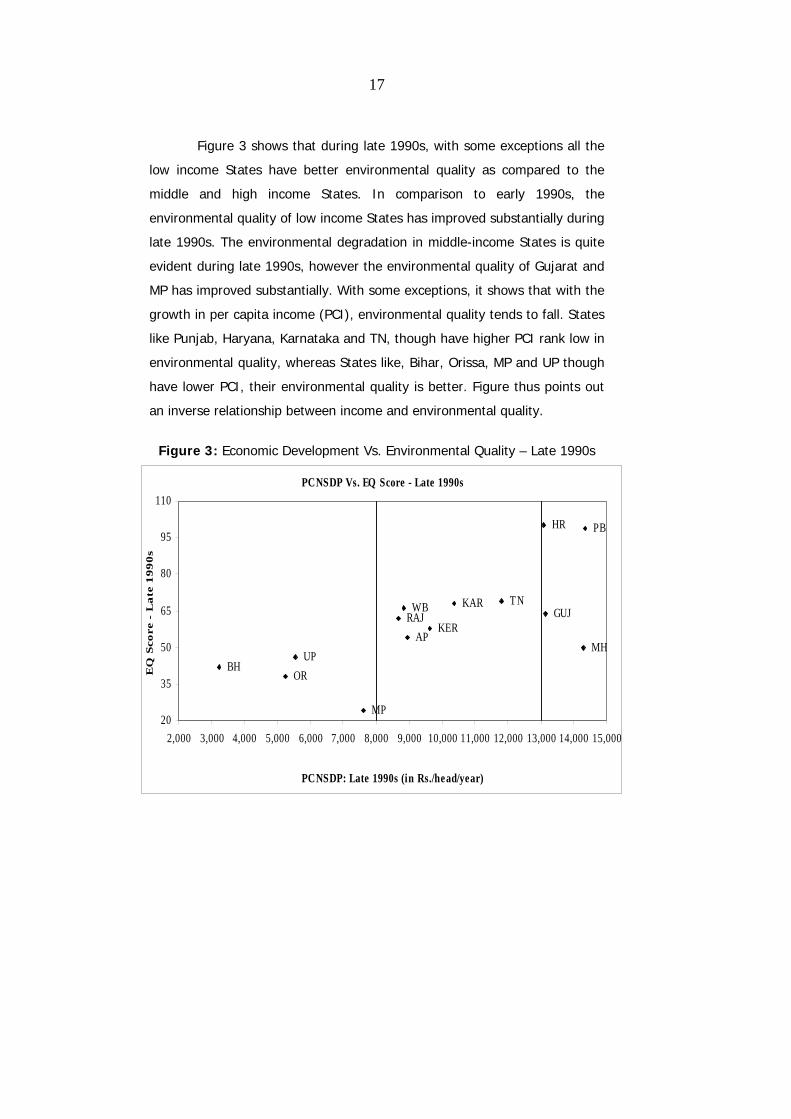
Figure 3 shows that during late 1990s, with some exceptions all the

low income States have better environmental quality as compared to the

middle and high income States. In comparison to early 1990s, the

environmental quality of low income States has improved substantially during

late 1990s. The environmental degradation in middle-income States is quite

evident during late 1990s, however the environmental quality of Gujarat and

MP has improved substantially. With some exceptions, it shows that with the

growth in per capita income (PCI), environmental quality tends to fall. States

like Punjab, Haryana, Karnataka and TN, though have higher PCI rank low in

environmental quality, whereas States like, Bihar, Orissa, MP and UP though

have lower PCI, their environmental quality is better. Figure thus points out

an inverse relationship between income and environmental quality.

Figure 3: Economic Development Vs. Environmental Quality – Late 1990s

PCNSDP Vs. EQ Score - Late 1990s

MP

BHOR

UP

RAJ

MH

GUJ

APKER

TNKARWB

PBHR

20

35

50

65

80

95

110

2,000 3,000 4,000 5,000 6,000 7,000 8,000 9,000 10,000 11,000 12,000 13,000 14,000 15,000

PCNSDP: Late 1990s (in Rs./head/year)

EQ

Sco

re -

La

te 1

99

0s

18

5.2 Verification for the EKC hypothesis for Indian States

To verify the EKC hypothesis, multivariate OLS regressions are

carried out.16 Before moving to estimation of EKC, it needs to be stated that

recent studies verifying EKC have used higher order specifications instead of

quadratic (see for example, Aldy, 2004). These researchers have argued that

one of the reasons for getting a peak outside the estimated function is

because of use of quadratic specification, which is restrictive. The present

study also suffers from the same limitation, as it could not use higher order

specifications due to data inadequacy. As a consequence, the restricted

regression function may give us only the first saddle point and not the

subsequent saddle point.

Table 6 reports the results and the saddle point for different variants

of model. From the table, it can be seen that there is non-linearity with

respect to per capita income (rows 2 and 3). With respect to controlling

variables, it can be easily seen that with the growing share of agriculture in

GSDP (AGR), the EQ declines. This is because with the rise in agricultural

intensity, pressure on land, water and forest resources start mounting up; as

a result EQ degrades. Similarly, increased share of workers in agriculture

(AGRWRK) also puts pressure on agricultural land and results in

environmental degradation.17 With respect to LITRU, as the rural literacy rate

increases EQS declines, which implies that spread of schooling and hence

literate population may be putting pressure on administration to manage

pollution and natural resources better.

16 Urbanisation, Share of Manufacturing in GSDP and Population Density though are important determinants of EQ, could not be used as they are found to be highly correlated with other explanatory variables. 17 Given high correlation between AGR and AGRWRK (≈ 0.5), they have been used interchangeably in the model.

19

Table 6: Verification of EKC

(Dependent Variable: Environmental Quality Score, EQS) (N=28) Explanatory Variable Coefficient Coefficient Coefficient Coefficient Coefficient Coefficient

2148.5* 2245.8* 1779.3* 2115.5* 1737.9* 2335.7* 1 Constant (1102.91) (1163.34) (965.44) (1058.27) (976.04) (1096.91)

-501.0* -529.2* -435.5* -495.7* -427.6* -551.4* 2 LNPCI (254.17) (270.33) (218.08) (243.6) (220.04) (253.41)

29.8* 31.8* 26.9* 29.9* 26.3* 32.9* 3 LNPCI2

(14.6) (15.45) (12.34) (13.93) (12.46) (14.58) 0.8* 0.9* 4 AGR

(0.39) (0.36) 0.27 0.4* 5 AGRWRK

(0.39) (0.18) -0.22 -0.26 -0.39* 6 LITRU

(0.36) (0.2) (0.19) 7 Adjusted R2 0.4 0.5 0.5 0.5 0.5 0.5 8 F-statistic 11.1 7.0 8.9 9.2 11.0 9.3

9 Durbin-Watson statistic 1.6 1.6 1.6 1.7 1.6 1.6

10 1st Saddle Point (Rs.) 4,462 4,135 3,234 3,989 3,347 4,343 Notes: Figure in the parenthesis shows White heteroskedasticity consistent standard error. * - Coefficient is significant at 10% level.

Row 10 giving the saddle point indicates that the point varies from

Rs. 3,234 to Rs. 4,462. This is the first saddle point showing a particular

PCNSDP above which environmental quality starts to decline. However,

except Bihar all other States already have PCNSDP higher than the saddle

point indicating that the States are on decreasing environmental quality. This

also suggests that EKC follows a slanting S-shaped curve, where

environmental quality may improve after reaching a particular per capita

income.

In Figure 4, both the actual and estimated EQS are plotted against

PCNSDP.18 The figure shows that after a certain point with the increase in

PCNSDP, EQS rises. The estimated second order polynomial trend shows

18 With the following specification ),( 2

ititit PCNSDPPCNSDPfEQS =

20

that, except Bihar all the other States have PCNSDP above the saddle point.

However, Orissa, AP and MP having low PCNSDP have comparatively better

environmental quality. Both Haryana and Punjab have high PCNSDP,

however their level of environmental degradation is also high. As compared

to Haryana and Punjab, Maharashtra and Gujarat have lower EQSs, but

maintain high PCNSDP. Both Rajasthan and Kerala are exceptions, as Kerala

maintains comparatively better environmental quality with a high level of

PCNSDP as compared to Rajasthan and vice versa.

Figure 4: PCNSDP vs. Actual & Estimated EQS

PCNSDP VS. Actual and Estimated EQS

68

BH1

BH2

PB2HR2

MP2

AP1OR1

MH2KER1

RAJ1

MP1UP1

GUJ2

HR1

10

20

30

40

50

60

70

80

90

100

110

2,000 4,000 6,000 8,000 10,000 12,000 14,000 16,000

PCNSDP (in Rs.)

EQS

& E

ST(E

QS)

EQS EST(EQS)

5.3 Economic Growth Vs. Environmental Degradation

The last part of the paper looks into what effect economic growth

has on change in environmental quality? To investigate, growth in GSDP is

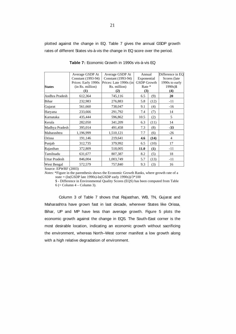
21

plotted against the change in EQ. Table 7 gives the annual GSDP growth

rates of different States vis-à-vis the change in EQ score over the period.

Table 7: Economic Growth in 1990s vis-à-vis EQ

States

Average GSDP At Constant (1993-94) Prices: Early 1990s

(in Rs. million)

Average GSDP At Constant (1993-94)

Prices: Late 1990s (in Rs. million)

Annual Exponential

GSDP Growth Rate *

Difference in EQ Scores (late

1990s to early 1990s)$

(1) (2) (3) (4) Andhra Pradesh 612,364 745,116 6.5 (9) 20 Bihar 232,983 276,883 5.8 (12) -11 Gujarat 561,660 738,047 9.1 (4) -16 Haryana 233,666 291,792 7.4 (7) 14 Karnataka 435,444 596,862 10.5 (2) 5 Kerala 282,050 341,209 6.3 (11) 14 Madhya Pradesh 395,014 491,458 7.3 (8) -33 Maharashtra 1,196,999 1,510,121 7.7 (6) -26 Orissa 191,146 219,641 4.6 (14) 4 Punjab 312,735 379,992 6.5 (10) 17 Rajasthan 372,809 518,005 11.0 (1) -11 Tamilnadu 631,677 807,387 8.2 (5) 18 Uttar Pradesh 846,004 1,003,749 5.7 (13) -11 West Bengal 572,579 757,840 9.3 (3) 16 Source: EPWRF (2003) Notes: *Figure in the parenthesis shows the Economic Growth Ranks, where growth rate of a

state = (ln(GSDP late 1990s)-ln(GSDP early 1990s))/3*100 $ - Difference in Environmental Quality Scores (EQS) has been computed from Table 6 (= Column 4 – Column 3).

Column 3 of Table 7 shows that Rajasthan, WB, TN, Gujarat and

Maharashtra have grown fast in last decade, wherever States like Orissa,

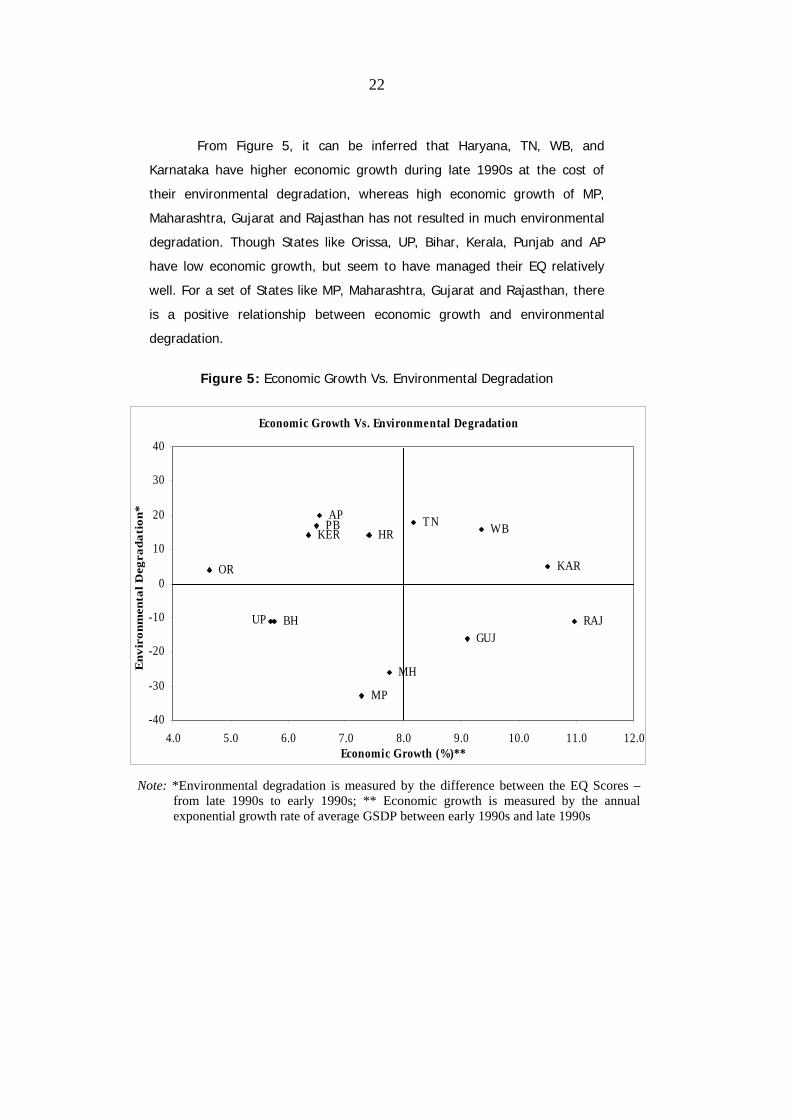
Bihar, UP and MP have less than average growth. Figure 5 plots the

economic growth against the change in EQS. The South-East corner is the

most desirable location, indicating an economic growth without sacrificing

the environment, whereas North–West corner manifest a low growth along

with a high relative degradation of environment.

22

From Figure 5, it can be inferred that Haryana, TN, WB, and

Karnataka have higher economic growth during late 1990s at the cost of

their environmental degradation, whereas high economic growth of MP,

Maharashtra, Gujarat and Rajasthan has not resulted in much environmental

degradation. Though States like Orissa, UP, Bihar, Kerala, Punjab and AP

have low economic growth, but seem to have managed their EQ relatively

well. For a set of States like MP, Maharashtra, Gujarat and Rajasthan, there

is a positive relationship between economic growth and environmental

degradation.

Figure 5: Economic Growth Vs. Environmental Degradation

Economic Growth Vs. Environmental Degradation

BHUP RAJGUJ

MH

MP

OR

PBAP

KER

KAR

WBTNHR

-40

-30

-20

-10

0

30

20

10

40

4.0 5.0 6.0 7.0 8.0 9.0 10.0 11.0 12.0Economic Growth (%)**

Env

iron

men

tal D

egra

dati

on*

Note: *Environmental degradation is measured by the difference between the EQ Scores – from late 1990s to early 1990s; ** Economic growth is measured by the annual exponential growth rate of average GSDP between early 1990s and late 1990s

23

6. Summary and Conclusions

The economic liberalisation process that began in India in 1991 has

resulted in States growing rapidly. A major consequence of this is

degradation in environmental quality. Under this backdrop this study

measures the environmental performance of 14 major Indian States by

ranking them under 8 broad environmental groups. These environmental

groups have been derived from a set of 63 environmental indicators by using

Principal Component Analysis method of factor analysis. The States are

ranked under each of the environmental groups (according to their score in

the first factor) and the ranks of the States are added up according to Borda

Rule to get the final environmental quality (EQ) score. Final environmental

ranks of the States are given on the basis of their EQ score, where States

having lower score get higher rank. The States are ranked for two time

periods - early 1990s (1990-1996) and late 1990s (1997-2001), and the

ranks are compared over period. The paper then investigates the relationship

between economic development and environmental quality (i.e.,

Environmental Kuznets Curve) using a multivariate regression analysis.

Data analysis shows that environmental ranks of the States vary

over time, which implies that environment has both spatial and temporal

dimensions. Ranking of the States across different environmental criteria

(groups) show that different States have different strengths and weaknesses

in managing various aspects of environmental quality. Thus, individual states

should adopt more focused environmental management practices based on

their local (at the most disaggregated level) environmental information

(conditions).

Results indicate that the relationship between per capita NSDP and

the environmental quality score is non-linear and follows a slanting S-shaped

curve, where barring Bihar, all the States are on the declining EQ region. The

low income States have better EQ as compared to their rich counterparts.

24

Both agriculturally and industrially developed States like Haryana, Punjab,

Gujarat and Maharashtra seem to have neglected their environmental issues.

The study could not find the point of inflexion, beyond which EQ will start

improving. However, taking a cue from developed countries and in

consonance with different MDGs (especially Target 919), there is a wide

scope to tunnel the EKC.

The study though could not compute the second inflexion point still

has wide policy implications. The quest for faster growth and aiming to

integrate with the world economy in nineties has forced many countries in

South Asia, South East Asia and Latin America to neglect their environment

and conservation of natural resources.

The study has few limitations. The analysis has been restricted to

only those 14 Indian States, for which various secondary environmental

information are available for both the periods. Thus, the analysis can be

extended by including more States. Similarly, the non-availability of data has

restricted the analysis for only two broad time periods. Subsequently this

analysis can be extended for more periods. Since a number of Indian States

are in the process of compiling environmental profile, the analysis can be

extended accordingly. Another limitation is use of only a restrictive quadratic

function to verify EKC, due to limited degree of freedom. The recent research

has attempted to include a higher order polynomial to verify EKC (see for

example, Aldy 2004). The main advantage of higher order polynomial is

finding both the saddle points, if the relation is slanting S. Thus, using more

observations can facilitate estimating a higher order polynomial and hence

second saddle point. Knowing the second saddle point also facilitate many

growing States to plan and tunnel the EKC accordingly.

19 Target 9 of MDG specifically stresses on integrating the principles of sustainable development into country policies and programmes and reverse the losses of environmental resources

25

APPENDIX – 1

Data Sources

Environmental Group

Data Sources

AIRPOL MoEF: National Ambient Air Quality Monitoring Programme Database TERI: TERI Energy Data Directory and Yearbook (TEDDY) – Various Years CSE: State of India’s Environment: The Citizens’ Fifth Report (Part II: Statistical Database)

INDOOR

RGI: Census of India 2001 – Tables on Houses, Amenities and Assets (Database Software) Garg and Shukla (2002)

GHGS RGI: Census of India 2001 – CensusInfo India 2001 (Version 1.0) – Database Software CMIE: India’s Energy Sector – Various Years TERI: TEDDY – Various Years RGI: CensusInfo India 2001 EPWRF (2003)

ENERGY

CSO: Compendium of Environmental Statistics – 2000 and 2002 FSI: State of Forest Reports – 1997, 1999 and 2001 MoEF: The State of Environment – India: 1999, 2001 CSE: Citizens’ Fifth Report RGI: CensusInfo India 2001

FOREST

EPWRF (2003) MoWR: Annual Report – Various Years CMIE: India’s Agriculture Sector – Various Years MoEF: National Rivers Water Quality Monitoring (NRWQM) Programme Database MoA: Annual Report – Various Years

WATER

CSE: Citizens’ Fifth Report CMIE: India’s Agriculture Sector – Various Years MoA: Annual Report – Various Years DoAHD&F: Livestock Census Data – 1992, 1997 and 2003 NPSP

RGI: Census of India 2001 – Tables on Houses, Amenities and Assets (Database Software)

LAND CMIE: India’s Agriculture Sector – Various Years

26

Notes:

CMIE: Centre for Monitoring Indian Economy, Mumbai

CSE: Centre for Science and Environment, New Delhi

CSO: Central Statistical Organisation, Ministry of Statistics and Programme

Implementation, Government of India (GoI), New Delhi.

DoAHD&F: Department of Animal Husbandry, Dairying & Fisheries, MoA, GoI,

New Delhi.

EPWRF: Economic and Political Weekly Research Foundation, Mumbai

FSI: Forest Survey of India, Ministry of Environment and Forest, GoI,

Dehradun

MoA: Ministry of Agriculture, (GoI), New Delhi

MoEF: Ministry of Environment and Forests, (GoI), New Delhi

MoWR: Ministry of Water Resources, (GoI), New Delhi

RGI: Office of the Registrar General, Director of Census Operation, Ministry

of Home Affairs, (GoI), New Delhi.

TERI: The Energy Resources Institute, New Delhi

27

APPENDIX – 2

DESCRIPTIONS OF ENVIRONMENTAL GROUPS (VARIABLES) & INDICATORS

AIR POLLUTION (12 indicators) • Maximum Concentration of NO2, SO2 and SPM in Residential and

Industrial Area (µg/m3): 1995 and 1999

INDOOR AIR POLLUTION POTENTIAL (12 indicators) • Monthly Per-Capita Expenditure (MPCE) on Bio-Fuels as a Percentage of

Total Expenditure on Fuels (%) for Rural and Urban Area: 1993-1994 and 1999-2000

• Percentage of Rural and Urban Households using Bio-fuels (Firewoods and chips, Dung cake) for cooking (%): 1993-1994 and 1999-2000

• Percentage of Rural and Urban Households Using Unsafe (Wood, Cowdung cake, others) Fuels: 1991

• Percentage of Rural and Urban Households using Unsafe Fuels for cooking (Firewood, Crop residue and Cow dung cake): 2001

GREEN HOUSE GASES EMISSIONS (8 indicators) • CO2 Equivalent GHGs (CO2, CH4, N2O) Emissions (100 Kg. /Person):

1990 and 1995

• CO2 Equivalent GHGs (CO2, CH4, N2O) Emissions (100 Tons/Rs. Crore of NSDP at Factor Cost (Current Prices)): 1990 and 1995

• CO2 Equivalent GHGs (CO2, CH4, N2O) Emissions (1000 Tons/Rs. Per Capita NSDP at Factor Cost (Current Prices)): 1990 and 1995

• Other GHGs (NOx, SO2) Emissions (10 Tons/Rs. Per Capita NSDP at Factor Cost (Current Prices)): 1990 and 1995

POLLUTION FROM ENERGY GENERATION AND CONSUMPTION (24 indicators) • Change in Electricity Sales to Agriculture as a Percentage of Total

Electricity Sales (Percentage points): 1990-91 to 1995-96 and 1995-96 to 1998-99

• Percentage Change in Number of Energised Pumpsets (%): 1990-91 to 1995-96 and 1995-96 to 1998-99

28

• Change in the Share of Thermal Electricity in Gross Electricity Generated (Percentage Points): 1990-91 to 1995-96 and 1995-96 to 1998-99

• Change in Per Capita Consumption of LPG, MG, K, HSD, LDO (Kg./Person): 1990-91 to 1995-96 and 1995-96 to 1998-99

• Change in Per Capita Consumption of Electricity (KWh/Person): 1990-91 to 1995-96 and 1995-96 to 1998-99

• Change in Per Capita Generation of Thermal Electricity (KWh/person): 1990-91 to 1995-96 and 1995-96 to 1998-99

• Energy Intensity of Agriculture (100 kWh/Lakh Rs.): 1995-96 and 1999-2000

• Percentage of Rural and Urban Households Having Access to Electricity: 1991 and 2001

• MPCE on Fuel & Lighting (Rs./month/head) Rural and Urban Areas: 1993-94 and 1999-2000

• Annual Percentage Increase in Motor Vehicles Number (given geographical area) during 1991-92 to 1995-96 and 1995-96 to 2000-2001

DEPLETION AND DEGRADATION OF FOREST RESOURCES (22 indicators) • Change in Dense Forest as a Percentage of Total Forest Area (in

percentage points) during 1995 to 1997 and 1999 to 2001

• Change in Open Forest as a Percentage of Total Forest Area (in percentage points) during 1995 to 1997 and 1999 to 2001

• Change in Total Forest Area as a Percentage of Geographical Area (in percentage points) during 1995 to 1997 and 1999 to 2001

• Change in Forest Area Per Thousand Person (in Sq. per 1000 Person) during 1995 to 1997 and 1999 to 2001

• Recorded Forest Area as a Percentage of Geographical Area (%): 1995 and 2001

• Common Property Forest Area* as a percentage of Total Forest Area: 1995 and 2001

• Common Property Forest Area* as a percentage of Geographical Area (%): 1995 and 2001

• Common Property Forest Area* Per 1000 Person (Sq. Km. Per 1000 Person): 1995 and 2001

• Percentage of Geographical Area under National Park (%): 1997 and 1999

29

• Percentage of Geographical Area under Wildlife Sanctuaries: 1997 and 1999

• Percentage Change in GSDP at Constant Prices from Forestry & Logging during 1993-94 to 1996-97 and 1996-97 to 1999-2000

• Note: * - Common Property Forest Area = Protected + Unclassed Forest Area

DEPLETION AND DEGRADATION OF WATER RESOURCES (20 indicators) • Percentage Share of Major & Medium Irrigation Potential Created upto

March 1992 and March 1997 to Ultimate Irrigation Potential (%)

• Percentage Share of Major & Medium Irrigation Potential Utilised upto March 1992 and March 1997 to Corresponding Potential Created (%)

• Percentage Share of Minor Irrigation Potential Created upto March 1992 and March 1997 to Ultimate Irrigation Potential (%)

• Percentage Share of Minor Irrigation Potential Utilised upto March 1992 and March 1997 to Corresponding Potential Created (%)

• Change in Percentage of Net Irrigated Area irrigated by Surface Water Sources (Canals, Tanks) during 1992-93 to 1995-96 and 1995-96 to 2000-2001 (Percentage points)

• Level of groundwater development (exploitation) (%), 1996 and 1998-99

• Change in Gross Irrigated Area (as a percentage of Gross-Cropped Area) (in percentage points): 1991-92 to 1995-96 and 1995-96 to 1998-99

• Pumsets Density (Number Per 1000 ha of Net Irrigated Area), 1994-95 and 1998-99

• Performance in Water Quality Monitoring (No of Monitoring Points for which data is available/Total No of Monitoring Point*100): 1997 and 2001

• Average Water Pollution (6=very good, 1=very bad): 1997 and 2001

NON-POINT SOURCE WATER POLLUTION POTENTIAL (14 indicators) • Fertilisers Consumption Per Hectare: (Kg./Hectares): 1995-96 and 1999-

2000

• Pesticides Consumption Per Hectare: (Kg./Hectares): 1995-96 and 1999-2000

• Change in Number of Livestock Per 1000 Hectares of Reporting Area (Number Per 1000 Hectare) during 1992 to 1997 and 1997 to 2003

30

• Change in Number of Persons Per 1000 ha of Reporting Area (Number/1000 ha) during 1991-92 to 1995-96 and 1995-96 to 1998-99

• Number of Persons Per 1000 ha of Reporting Area (Number/1000 ha): 1995-96 and 1998-99

• Change in Gross Irrigated Area (as a percentage of Gross-Cropped Area) (in percentage points): 1991-92 to 1995-96 and 1995-96 to 1998-99

• Gross Irrigated Area (Percentage of Gross-Cropped Area): 1995-96 and 1998-99

PRESSURE AND DEGRADATION OF LAND RESOURCES (14 indicators) • Change in Land Not Available for Cultivation (as a percentage of

reporting area) (in percentage points): 1991-92 to 1995-96 and 1995-96 to 1998-99

• Change in Fallow Land (as a percentage of reporting area) (in percentage points): 1991-92 to 1995-96 and 1995-96 to 1998-99

• Change in Net Sown Area (as a percentage of reporting area) (in percentage points): 1991-92 to 1995-96 and 1995-96 to 1998-99

• Change in Area Under Foodgrains (as a percentage of Gross Cropped Area) (in percentage points): 1991-92 to 1995-96 and 1995-96 to 1998-99

• Change in Gross Irrigated Area (as a percentage of Gross-Cropped Area) (in percentage points): 1991-92 to 1995-96 and 1995-96 to 1998-99

• Change in Gross Cropped Area (as a percentage of Reporting Area) (in percentage points): 1991-92 to 1995-96 and 1995-96 to 1998-99

• Change in Area Cultivated More than Once (as a percentage of Gross Cropped Area) (in percentage points): 1991-92 to 1995-96 and 1995-96 to 1998-99

31

References

Adriaanse, A., Bryant, D., Hammond, A.L., Rodeburg, E. and Woodward, R.

(1995), ‘Environmental indicators: a systematic approach to

measuring and reporting on environmental policy performance in the

context of sustainable development’, Washington D.C., World

Resources Institute.

Adriaanse, A. (1993), ‘Environmental policy performance indicators: a study

of the development of indicators for environmental policy in the

Netherlands’, The Hague, SDU Publishers.

Agarwal, Bina (1995), ‘Gender, Environment and Poverty Interlinks in Rural

India: Regional Variations and Temporal Shifts, 1971-1991’,

Discussion Paper No. 62, Switzerland, United Nations Research

Institute for Social Development.

Aldy, J.E. (2004), ‘An Environmental Kuznets Curve Analysis of U.S. State-

Level Carbon Dioxide Emissions’, Working Paper, Department of

Economics, Cambridge, USA, Harvard University.

Andreoni, J. and Levinson, A. (2001), ‘The simple analytics of the

Environmental Kuznets Curve’, Journal of Public Economics, Vol. 80,

No.1, 269-86.

Baldwin, R. (1995), ‘Does sustainability require growth?’, in Goldin, I. and

Winters, L.A. (eds.), ‘The Economics of Sustainable Development’,

Cambridge, UK, Cambridge University Press, pp. 19–47.

Bruvoll, A. and Medin, Hege (2003), ‘Factors Behind the Environmental

Kuznets Curve: A Decomposition of the Changes in Air Pollution’,

Environmental and Resource Economics, Vol. 24, No. 1, 27-48.

32

Carson, R.T., Jeon, Y. and McCubbin, D.R. (1997), ‘The relationship between

air pollution emissions and income: US Data’, Environment and

Development Economics, Vol. 2, No. 4, 433-50.

Convention on Biological Diversity (CBD): Undated, Global Biodiversity

Outlook, Montreal, Quebec, Canada, UNEP, available at

http://www.biodiv.org/gbo/annex.asp?ann=1. accessed on

12.02.2005

Dasgupta, Partha (2001), ‘Human Well-Being and the Natural Environment’,

New Delhi, Oxford University Press.

de Bruyn, S.M., van den Berg, J.C.J.M. and Opschoor, J.B. (1998), ‘Economic

growth and emissions: reconsidering the empirical basis of

environmental Kuznets curve’, Ecological Economics, Vol. 25, 161-75.

Dinda, S. (2004), ‘Environmental Kuznets Curve Hypothesis: A Survey’,

Ecological Economics, Vol. 49, 431-55.

EPWRF (2003), ‘Domestic Product of State of India: 1960-61 to 2000-01’,

Database Software.

Esty, D.C., Levy, M., Srebotnjak, T. and de Sherbinin, A. (2005), ‘2005

Environmental Sustainability Index: Benchmarking National

Environmental Stewardship’, New Haven, Yale Center for

Environmental Law & Policy.

Garg, Amit and Shukla, P.R. (2002), ‘Emission Inventory of India’, New Delhi,

Tata McGraw-Hill Publishing Company Limited.

Grossman, G.M. and Krueger, A.B. (1995), ‘Economic Growth and the

Environment’, Quarterly Journal of Economics, Vol. 110, 353-78.

Jha, Raghbendra and Bhanu Murthy, K.V. (2001), ‘An Inverse Global

Environmental Kuznets Curve’, Departmental Working Papers: 2001-

33

02, Division of Economics, RSPAS, Canberra, Australia, Australian

National University.

Jones, L., Fredricksen, L. and Wates, T. (2002), ‘Environmental indicators’,

Fifth Edition, The Fraser Institute, available at

http://www.fraserinstitute.ca/shared/readmore.asp?snav=pb &id

=314. accessed on 12.02.2005

Kathuria, Vinish (2004), ‘Impact of CNG on Vehicular Pollution in Delhi: A

Note’, Transportation Research Part D, Vol. 9, 409-17.

Kathuria, Vinish (2002), ‘Vehicular Pollution Control in Delhi, India’,

Transportation Research – Part D, Vol. 7, No. 5, 373-87.

Kothari, Ashish (1996), ‘Structural Adjustment vs. India's Environment’,

Proceedings of the Annual Meetings, Honolulu, Association for Asian

Studies.

Nadkarni, M.V. (2000), ‘Poverty, Environment, Development: A Many

Patterned Nexus’, Economic and Political Weekly, April 1, 2000,

1184-90.

Panayatou, T. (1993), ‘Empirical tests and policy analysis of environmental

degradation at different stages of economic development’, World

Employment Research Programme, Working Paper No. WP238,

Technology and Employment Programme, Geneva, International

Labour Office.

Pezzey, J. (1989), ‘Economic Analysis of Sustainable Growth and Sustainable

Development’, Environment Department Working Paper No 15,

Washington D. C., The World Bank.

Rogers, Peter, Jalal, Kazi F., Lohani, Bindu N., Owens, Gene M., Yu, Chang-

Chung, Christia, M. and Dufournaud, Jun B. (1997), ‘Measuring

34

Environmental Quality in Asia’, London, U.K., Harvard University

Press and ADB.

RIVM/UNEP: undated, ‘Global Environment Outlook (GEO-3)’, Bilthoven, The

Netherlands, National Institute of Public Health and the Environment

(RIVM), UNEP, available at http://arch.rivm.nl/env/int/geo/.

accessed on 12.02.2005

Selden, T.M. and Song, D.S. (1994), ‘Environmental quality and

development: is there a Kuznets curve for air pollution emissions?’,

Journal of Environmental Economics and Management, Vol. 27, 147-

62.

Shafik, N. and Bandyopadhyay, S. (1992), ‘Economic growth and

environmental quality: time-series and cross-country evidence’,

World Bank Policy Research Working Paper No. WPS 904,

Washington D. C., The World Bank.

Stern, D.I. (1998), ‘Progress on the Environmental Kuznets Curve’,

Environment and Development Economics, Vol. 3, 175-98.

World Development Indicator (2004), available at

http://www.worldbank.org/data /countrydata/countrydata.html

accessed on 20.02.2005.

World Wildlife Fund (WWF) (2002), ‘WWF's Living Planet Report 2002’,

Switzerland, WWF International available at

http://www.panda.org/news_facts

/publications/general/livingplanet/lpr02.cfm. accessed on

12.02.2005.