Electronic copy available at: http://ssrn.com/abstract=2349903

1

Is Financialization Killing Commodity Investments?

Adam Zaremba

Poznan University of Economics

adam.zaremba@ue.poznan.pl

Abstract

Although the financialization of commodity markets has recently become a broadly discussed

phenomenon, its implications for commodity investors remain unknown to a large extent. This paper

focuses on whether the potential benefits of passive investment strategies in the commodity futures

markets would be expected to continue with the increased financialization of the commodity futures

markets. Firstly, a regression analysis was conducted in order to examine the correlation between

financialization and the disappearance of roll yields. Secondly, after finding such a correlation, we

assume that this correlation was driven by the increased financialization causing the decline in roll

yields. Thirdly, simulation-based methods were implemented to examine the revised efficient

frontiers after accounting for the potential impact of financialization on roll yields. Empirical research

was based on returns on various asset classes and other related variables over the period between

1990 and 2012. The computations indicate that market financialization may have resulted in a decline

in expected roll returns. This decrease in roll yields, should it continue, is of a potential magnitude

that this would undermine the legitimacy of including commodity futures in traditional stock-and-bond

portfolios.

Keywords: commodities, financialization, roll yields, mean-variance spanning test, strategic asset

allocation.

JEL codes: G11, G12, G13.

Electronic copy available at: http://ssrn.com/abstract=2349903

2

Arguably, commodity futures once were thought to serve as a holy grail for hedging stock-market

portfolios. Nearly a decade ago several crucial studies raised the possibility that commodity

investments could increase the return expected on an investment portfolio while simultaneously

reducing its risk. The publications were quickly followed by an explosion of various commodity

investment vehicles and a significant inflow of capital into commodity markets. “The increase in

investor activity” was subsequently described as the “financialization” of commodity markets

[Domanski and Heath 2007]. Since then, the landscape of commodity markets has drastically changed.

Once a market of refineries, mines and farms, it has been transformed into the market of hedge funds,

exchange-traded funds and commodity advisors. Although the role of speculators was recognized

a long time ago, never before it was so important.

Effects of financialization on commodity markets are still the subject of discussion. Some researchers

believe that they have undergone a deep and structural change. The literature concerning this subject

usually indicates an increased correlation between commodities and other asset classes [TDR 2009,

Tang and Xiong 2012, Silvennoinen and Thorp 2009], and changes within the term structure of

commodity markets [Mayer 2010, Tang and Xiong 2012, Vdovenko 2013, Brunetti and Reiffen 2011,

Mou 2011]. Some research strands also revealed the emergence of price bubbles [Masters 2008,

Gilbert 2009, 2010, Einloth 2009]; however, other studies reached different conclusions in this matter

[Plante & Yucel 2011; Buyuksahin 2012; Sanders, Irwin & Merrin 2009; Aurelich, Irwin & Garcia

2013; Huntington et al. 2014; Cevik & Sedik 2011; Irwin 2013].

Financialization is a relatively new phenomenon; thus, there are still no firm answers as to whether

and how financialization may have changed commodity futures markets. Additionally, the scope of the

effects of financialization on investment conditions and opportunities in commodity markets is still

unknown even though this knowledge is crucial from the investors’ perspective.

This paper aims to investigate a single aspect of the consequences of financialization – i.e., changes in

future roll returns – and to assess implications of this phenomenon for commodity investors. The

analysis is performed from the perspective of ordinary US investors who maintain their funds in stock

Electronic copy available at: http://ssrn.com/abstract=2349903

3

and bond market. In other words, this paper makes an attempt to prove whether investing in

commodities in the view of financialization and its impact on the term structure is still economically

justified.

The paper is organized in several parts and structures as follows. First, the characteristic properties of

commodity investments are described, together with the listing of methods to obtain exposure to

commodities and the description of their key return sources. The existing literature referring to the

potential benefits of commodity investments is also reviewed. Secondly, the concept of

financialization is defined and an independent, proprietary research hypothesis is developed. The third

section includes a description of research methods and data sources. A new measure of the level of

financialization is also introduced. Further, the results of an empirical, twofold analysis are presented.

Its first stage includes the performance of a regression analysis in order to assess the potential impact

of financialization on commodity markets. In the second stage, we adjust expected commodity futures

returns based on this regression and examine what this decline in expected returns would mean for a

diversified portfolio’s efficient frontier of stocks, bonds, and commodity investments. The empirical

research is based on returns on various asset classes and other related variables over the period

between 1990 and 2012. Finally, the paper ends with concluding remarks and recommendations for

future research.

Commodities as Investment Assets

One of the key distinguishing features of commodities as an asset class is the variety of methods

available to investors for obtaining exposure to them. In practice, there are three basic methods

[Idzorek 2007]: direct physical purchase, commodity related stocks, and commodity futures.

Each of the above mentioned methods of exposure has its own risk and return characteristics. Physical

investment is simply too impractical as some commodities (particularly cattle and agricultural

commodities) tend to perish quickly, even those that do not require complicated storage and

4

transportation. In fact, the only exceptions are precious metals such as gold or silver. Other types of

direct physical investment are still fairly rare1.

Commodity-related stocks seem to be part of a broader asset class of equities rather than commodities.

They provide exposure to business skills of managers and specific factors related to companies, and in

many cases may even hedge out their commodity exposure. Therefore, some analyses may often

indicate stronger correlation between commodity-related stocks and equities than between such stocks

and commodities themselves. Gorton and Rouwenhorst [2006] created a portfolio of commodity

stocks on the basis of SIC codes and investigated its behavior over the period of 41 years. The

correlation between the portfolio and the commodity futures index was 0.40, whereas in the case of

S&P 500 it accounted for 0.57. Moreover, it also appears that commodity stocks not only resemble

equities rather than commodities, but also result in lower rates of return and are not explicitly defined

as an efficient inflation hedge [Gorton and Rouwenhorst 2006]. As a result, many researchers

conclude that a portfolio of commodity-related stocks is not a sufficient method of obtaining exposure

to commodities.

The third method, widely recognized as the most appropriate one, comprises direct investment in

a commodity futures portfolio. This can be achieved either by hiring a professional portfolio manager

(CTA) to actively manage the portfolio (managed futures) or through a passive long position in

a commodity index. In a later section of this paper the focus shall be placed upon the second method

as the one that it is free from influence of active investment strategies.

The passive index investment defines first and foremost the purchase of a portfolio of fully

collateralized commodity futures being systematically rolled upon or prior to their maturity.

According to previous studies in this field, such investments are of particular interest to traditional

equity and bond investors due to a variety of distinctive features of commodities: the positive

skewness of return distributions [Deaton and Laroque 1992, Armstead and Venkatraman 2007], the

1 A notable exceptions could be also farmland and timberland ownership at the institutional level, which is

sometimes regarded as a type of commodity investments. The benefits of farmland and timberland investing are

investigated among others by Hennings et al. [2005], Scholtens and Spierdijk [2010], Painter [2010], or

Koeniger [2014].

5

mean-reverting feature of commodity prices , [Sorensen 2002], the hedging properties against inflation

[Bodie 1983; Gorton and Rouwenhorst 2006; Froot 1995; Till and Eagleeye 2003a; Till and Eagleeye

2003b; Akey 2007], the potential long-term positive risk premium [Till 2007a, Till 2007b, Till 2007c],

and the low correlation with traditional asset classes such as stocks or bonds [Ankrim and Hensel

1993, Becker and Finnerty 1994, Kaplan and Lummer 1998, Anson 1999, Abanomey and Mathur

2001, Georgiev 2001, Gorton and Rouwenhorst 2006].

Risk Premium of Commodities and Its Role in Portfolio Optimization

The two abovementioned characteristic features of commodity futures, i.e. low correlation and long-

term risk premium, translate into particular attractiveness of these futures in terms of strategic asset

allocation. Since the 1970s researchers [Till 2007a] have shown interest in this field; thus, the subject

literature is relatively in-depth. The below papers are presented in chronological order.

Initial studies focused on the US agricultural market, but did not deliver promising results. Dusak, who

analyzed listings of singular commodities over the period between 1962 and 1967, was not able to

prove the existence of positive risk premium in 1973 [Dusak 1973]. Breakthrough in this field shall be

attributed to Greer [1978], who treated commodities as an asset class. Greer showed that risks

associated with commodity investment may be effectively reduced through full collateralization. On

the basis of a price index developed between 1960 and 1976 he calculated that an investment in

commodity futures had performed better than an equity investment, particularly by delivering higher

returns and lower drawdowns than equities. In their most often cited paper of 1980, Bodie and

Rosansky argued that commodity futures have a positive risk premium [Bodie and Rosansky 1980].

They showed that a risk premium was present in 22 out of 23 analyzed markets over the period

between 1950 and 1973; however, the statistical significance of results was rather low. It is probably

due to relatively high volatility of single futures; therefore, Bodie and Rosansky performed similar

computations also for a commodity index delivering statistically significant rates of return. Similar

results were later obtained by Bodie [1983], Carter et al. [1983], Chang [1985] and Fama and French

[1987]. Bessembinder [1992] noted that the presence and amount of risk premium is dependent on the

6

term structure whereas Bjornson and Carter [1997] observed that the risk premium correlates with

macroeconomic factors: economic activity, inflation and interest rates. Historically, expected returns

to commodities were lower during times of high interest rates and expected inflation. Similar

conclusions were drawn by Chong and Miffre [2006]. Kaplan and Lummer [1998], who focused on

fully collateralized investments in S&P GSCI index, noted that, historically, index investments

achieved higher returns, but also bore higher risks, than investments in equities. Returns in commodity

markets were also a subject of interest to Greer [2000], Till [2000a, 2000b] and Dunsby et al. [2008].

The latest studies on the risk premium of commodities emphasize the difference between risk

premiums with respect to indices and to single commodities. Garcia and Leuthold [2004] found the

presence of risk premium for indices over the period between 1982 and 2004; however, they haven’t

reached unequivocal conclusions concerning single instruments. According to calculations conducted

by Anson [2006], commodity portfolios achieved higher return than bonds and equities between 1970

and 2000, but at a slightly higher risk. Erb and Harvey [2006a] believe that the acceptance or rejection

of the risk premium hypothesis is highly dependent on research data and research methodology.

A significant breakthrough was experienced in 2004 upon the first publication of Gorton’s and

Rouwenhorst’s working paper. Their article entitled “Facts and Fantasies about Commodity Futures”

[Gorton and Rouwenhorst 2006] is widely recognized as providing the credibility for the emergence of

commodities as an asset class [Rogers 2007, Authers 2010]. Gorton and Rouwenhorst found the

statistically significant presence of risk a premium for 36 commodities over the period between 1959

and 2004. According to them, the portfolio performed about equal to equities and its Sharpe ratio was

even higher due to a lower standard deviation. And conversely, they were unable to confirm

statistically significant rates of return for single markets. A number of later papers confirmed the

findings of Gorton and Rouwenhorst. Kat and Oomen [2007a] did not find risk premiums in a broad

spectrum of 42 commodities over the period between 1965 and 2005; whereas, Scherer and He [2008]

found the presence of risk premiums between 1989 and 2006for Deutsche Bank indices, but not for all

constituents. Long-term return rates on indices were also found by Hafner and Heiden [2008] in their

analysis for the period between 1991 and 2006, by Füss et al. [2008] in the analysis for the period

7

between 2001 and 2006, as well as Shore [2008], who investigated the S&P GSCI index over the

period between 1969 and 2006. Positive rates of return, higher than return rates of stocks and bonds,

were also documented by Nijman and Swinkels [2008]; however, they also observed historically

higher volatility than in the case of traditional asset classes. Risk premiums in commodity markets

were also analyzed by Gorton et al. [2012].

Another important aspect of commodity research is diversification properties and the resulting benefits

for an investment portfolio. The first scientific analysis of this kind is believed to be performed by

Greer in 1978. In his pioneering work [Greer 1978] Greer showed that a rebalanced portfolio of

commodities, stocks and bonds delivers more stable and higher rates of return than a pure bond and

stock portfolio. Bodie and Rosansky [1980] noted that allocation of 40% of portfolio to commodity

futures had resulted in risk reduction and a simultaneous increase in expected return. Similar

conclusions on the historical benefits of commodity investing were later drawn by Jaffe [1989],

Satyanarayan and Varangis [1994], Froot [1995], Kaplan and Lummer [1998], Fortenberry and Houser

[1990], Jensen et al. [2000], Woodard et al. [2006] and Anson [2006]. In his calculations conducted

for Ibbotson Associates, Idzorek [2006] showed that there had been a low correlation between

commodities and stocks and bonds as commodities, contrary to stocks and bonds, were positively

related to inflation. Kat and Oomen [2007a] showed that a partial allocation to the GSCI had improved

a portfolio’s Sharpe ratio; whereas, according to Woodard [2008], between 1989 and 2006

commoditiy futures exhibited a positive risk premium, which was impossible to be explained in terms

of returns on stocks or bonds. The shift in the efficient frontier, resulting from the commodity

allocation, was also discussed by Scherer and He [2008] with several important caveats, and by Shore

[2008]. However, the most interesting paper among the latest ones is the paper of Heidon and

Demidova-Manzel [2008], who analyzed return patterns of portfolios comprising equities, sovereign

and corporate bonds, and real estate properties between 1973 and 1997. They concluded that investors

should allocate between 5% and 36% of their portfolio to commodities. Other recent studies

concerning the benefits of commodities in terms of strategic asset allocation are those conducted by

Doeswijk et al. [2012] and Bekkers et al. [2012].

8

Sources of Return in Commodity Futures Market

One essential question with regard to this paper is: what are the sources of return in commodity futures

markets? An answer to this question could be formed on the basis of an accounting perspective or

from an economic perspective.

In respect to the accounting perspective, there are three key sources of return in commodity futures

market2. The first one is spot return (price return), in its fundamental meaning being the component of

return that arises from changes in nearby prices [Shimko and Masters 1994]. Interestingly, early

studies demonstrate that long term spot returns are close to zero [Grili and Yang 1988]. In other

words, changes in spot prices have not resulted in significant, long-term real (inflation-adjusted)

returns; thus, the existence of risk premiums would have to be due to other factors, such as pricing of

commodity futures, strategy design or portfolio composition. Similar evidence was found by

Cuddington [1992], Cashin et al. [1999], Cashin and McDermott [2001], and Burkart [2006], and

confirmed by Gorton and Rouwenhorst [2006], and Erb and Harvey [2006a] in their most cited papers

on commodity investments. Interesting conclusions were also drawn by Anson [2006] who believed

that, despite the fact that long-term risk premium is determined by other factors, it is the spot return

that is responsible for the diversification properties of commodities.

The second source of return is collateral yield, inseparably bound to the full collateralization of total

return indices. Historically, collateral yields constituted a relatively high percentage of total return due

to particularly high inflation and interest rates in the 1970s and 1980s. However, based on simple

arithmetical principles, collateral yields are, obviously, no reason for the existence of risk premiums.

The third source of return, apparently the most important one, is roll yield3. The roll return is the return

from the passage of time (carry) assuming the term structure of futures contract does not change. If

a market is in a backwardation (downward sloping term structure), the return from rolling up the

curve (for example, selling a 3-month futures after 1 month as a 2-month future) is positive, while it is

2 The split of historical commodity returns into three sources (spot returns, roll yields and collateral yields) can

be found for instance in the papers of Markert and Zimmermann [2008], Fuss et al. [2008], Hafnem et al. [2008],

Mezger [2008] and Shore [2008]. 3 The terms “roll return” and “roll yield” are interchangeable in this paper.

9

negative if markets are in contango (upward sloping term structure). The greater the slope of the term

structure, the more pronounced these effects are [Scherer and He 2008, p. 257]. If market experiences

backwardation, the new price is lower, while in the case of contango, it is higher. In respect to

commodity index computation, roll return constitutes the difference between excess return and spot

return.

Many researchers believe that roll return is the key factor in determining long-term returns on

particular commodities [Nash 2001, Till and Eagleeye 2003a, Kat and Oomen 2007a, Kat and Oomen

2007b]. According to Erb and Harvey [2006], 92% of cross-sectional variation in excess return on

commodities is to be explained by roll returns. This was, in fact, confirmed by Markert and

Zimmermann [2008]. Their regression yielded an R-squared of 88.6%.

Furthermore, besides the three aforementioned sources of return, there are also other index-specific

factors, such as return on diversification (interpreted by Willenbrock as a return on rebalancing

[2011]), which is also demonstrated and/or discussed in several other papers [Erb and Harvey 2006a,

Erb and Harvey 2006b, Scherer and He 2008, De Chiara and Raab, Plaxco & Arnott 2002].

From an economic perspective, there are several theories explaining pricing in commodity futures

markets and defining possible sources of a risk premium. One of the most prominent, is the “theory of

normal backwardation”, dating back to Keynes [1930] and Hicks [1939]. According to this theory the

commodity futures markets provide some traits of insurance. If producers hedge their production with

short positions, they must compensate long risk-averse investors with a risk premium. The described

concept evolved later into a more general form called “hedging pressure hypothesis”, according to

which, the risk premium may result from either producers or consumers, depending upon which type

of market participant exerts stronger hedging pressure. In a nutshell, in accordance with the hedging

pressure hypothesis, in commodity futures markets, the risk is transferred from hedgers to speculators,

who earn a premium for bearing the risk. The hedging pressure hypothesis was later incorporated in

many models and confirmed by many researchers [Houthakker 1957, Cootner 1960, Chang 1985,

10

Bessembinder 1992, De Roon et al. 2000, Anderson and Danthine 1981]. Supporting evidence was

also revealed by recent papers, including those of Basu and Miffre [2013], and Acharaya et al. [2013].

According to this theory, the general formula defining the futures contract price is the following one:

[ ] (1)

where rp denotes risk premium and ET [ST ] is an expected price at time T. An interesting observation

in this model is the fact that neither the risk premium nor the expected spot price is directly visible.

Markert and Zimmermann [2008] provided an interesting derivation that shows the link between the

risk premium and the common accounting return decomposition into spot, roll and collateral yields,

and the convenience yield. According to Markert and Zimmerman, roll yield (ry) may be described as:

, (2)

where rp is the risk premium and αS denotes the expected growth rate of spot price. In other words, if

expected growth rate of a spot price is equal to zero, then ex-post roll return is equal to risk premium.

In addition to the concept described above, there are several other theories. Among them the most

popular is the theory of storage4. It assumes that a holder of a physical commodity has some

indispensable benefits (e.g., lower risk in the case of commodity shortage in the market due to

production stoppage or increased demand) that a holder of futures is deprived of. Introduced by Kaldor

[1939], the term “convenience yield” defines additional profits on the part of a physical commodity

4 This idea originated from Kaldor [1939] and was later developed and interpreted by many other researchers

[Working 1948, Working 1949, Brennan 1958, Telser 1958, Telser 1960, Helmuth 1981, Brennan 1991, Erb and

Harvey 2006a, Till 2008, Spurgin and Donoue 2009]. The theory of storage appears to have solid foundations of

empirical research as it was proved, e.g. by Fama and French [1988], and Ng and Pirrong [1994]. Recent studies

in this field include papers prepared by Dinceler et al. [2006] and Gorton et al. [2012], providing solid support

for the theory of storage.

11

holder5. The concepts other than the theory of storage and the hedging pressure hypothesis are not so

broadly recognized and extensively documented6.

Market Financialization and Hypothesis Development

In recent years we experienced a massive influx of capital into commodity-futures-related products. It

is said that at least 100 billion dollars moved into commodity futures markets between 2004 and 2008

[Irwin and Sanders 2011]. Trading volume increased dramatically and the presence of financial

investors has also been constantly increasing. According to the CFTC, the share of open interest held

by non-commercial market participants surged from 15% in the beginning of 1990 to over 42% in the

end of 2012. Domanski and Heath [2007] coined the “financialization” term to describe the growing

presence and importance of financial institutions in commodity markets. Changes do not seem to be

temporal, but rather structural [Irwin and Sanders 2012].

One could reasonably assume that such profound changes could have somehow altered the functioning

of commodity markets. Lots of studies have been conducted in this field. As has already been noted,

there are several structural changes discussed in research papers that could have taken place in

commodity markets as the result of financialization, including the emergence of price bubbles,

increased correlation among commodities and with other asset classes, as well changes in the term

structure of commodity markets [Mayer 2010, Tang and Xiong 2012, Vdovenko 2013, Brunetti and

Reiffen 2011]. Structural changes in commodity markets might be of high importance for commodity

investors. The theories explaining commodity risk premiums, as described above, argue that the risk

premium compensates for the risk transfer from hedgers to investors (speculators). If the amount of

hedging is relatively constant and the number of investors grows, the share of the risk premium per

investor simply shrinks. In other words, financialization may result in the decrease in risk premiums

5 It is worth pointing out that the storage and hedging pressure hypotheses are not mutually exclusive [Fama and

French 1988]. Several attempts have been made to connect both concepts (e.g. Cootner [1967], Khan et al.

[2008]). The aim was finally reached by Hirshleifer [1990] who, actually, synthetized the papers of Keynes

[1930] and Working [1949]. According to Gorton et al. [2012] hedging demand correlates with inventory levels,

implying that time-varying hedging pressure is dependent on the storage risks [Gorton et al. 2012]. 6 Other theories include for example the theory of rational expectations [Hicks 1939, Hurwicz 1946], market

segmentation, liquidity preference [Spurgin and Donohue 2009], the option theories [Litzenberg and Rabinowitz

1995, Milonas and Thomadakis 1997, Zulauf, Zhou and Robert 2006]. The detailed description of these theories

is beyond the scope of these study.

12

for long-position commodity investors. If we take the risk premium as described as in equation (2),

then the decline in risk premium, ceteris paribus, might imply the decrease in roll yields. As a result of

commodities financialization, the roll yields constituting a substantial component of long-term returns

on commodities might be structurally lowered in the future. If this statement holds true, this could be

detrimental for future commodity investments. Lower long-term risk premium may put into question

the usefulness of commodities as an asset class, either in terms of a portfolio enhancer or as

a standalone investment.

It should be noted that it is not only the reduction of roll yields that may jeopardize the rationale for

including commodities in a diversified portfolio. The other impediment may be the decrease of

profitability of strategies based on term-structure [Zaremba 2014a]. Furthermore, the increase in

correlation between the commodities as an asset class and equities, investigated by for example Tang

and Xiong [2014], could have negative impact on the benefits of commodity investments [Zaremba

2014b]. However, whether the changes in correlations are related to financialization is still an issue in

an ongoing debate. Norrish et al. [2014] argue that the level of correlations with other asset classes

was actually declining in year 2014. Also Daskalaki and Skiadopoulos [2011] contest the benefits of

commodities in a portfolio. These authors test the hypothesis that commodities should be an integral

part of any investment portfolio because they offer diversification which results from negative

correlations with traditional asset classes: stocks and bonds. The period examined is 1989-2009. The

authors conclude that investor utility is maximized in a traditional portfolio and risk-adjusted returns

fall after the addition of commodities. In other words, the addition of commodities does not offer value

in terms of higher risk-adjusted returns for investors. This observation is consistent for longer and

shorter periods with the exception of the short commodity boom period of 2005–2008. Daskalaki and

Skiadopoulos relate the erosion of diversification benefits to the rising investment of funds in

commodity indices.

13

Data Sources and Research Design

In this paper the empirical analysis is divided into two stages. First of all, its aim is to investigate

whether an increased presence of commodity investors translates into the decrease in roll yields and to

assess the size of its impact. Secondly, the paper will investigate whether commodities as an asset

class are still beneficial as a portfolio enhancer, given a potential continued decrease in roll yields.

The paper will do so by evaluating the change in the efficient frontier when adding commodities, both

with and without reduced roll yields. The reduction in roll yields is calculated from the empirical link

between the increase in financialization and the reduction in roll yields. We construct both a classic

mean-variance efficient frontier as well as one taking into consideration the skewness and kurtosis of

portfolio returns. We also use a Monte Carlo method to examine the potential change in a portfolio’s

Sharpe ratio by including commodities, using both historical returns and reduced returns. Like the

efficient frontier analysis, we calculate classic Sharpe ratios and modified Sharpe ratios, with the latter

ratio providing a measure of return-per-extreme-risk.

In order to study the relationship between roll returns and investor presence, a simple OLS regression

was performed with the use of JP Morgan Commodity Curve Index (JPMCCI) as a proxy for returns

on commodities as an asset class. Currently there are many indices available; however, the JPMCCI

has been chosen for several reasons. First and foremost, it is dated back to December 1989; thus, it

represents a relatively long time series. Secondly, it is calculated in total, excess and spot return

convention. Thirdly, it avoids a common front-run bias as it exposes an index investor to a full

commodity curve. Then, its constituents are weighted in accordance with open interest, arguably

a good representation of investors’ universe. Finally, it does not assume any sophisticated active

portfolio allocation methods that could distort pure returns on commodities as an asset class. It should

also be noted that the JPMCCI is used to represent investment commodities as an asset class, not as an

investment in a particular commodity index. Therefore, the results may differ in terms of other

commodity indices focused merely on a specific part of commodity curve, or which employ an active

allocation strategy.

14

In our study, at each time t forward looking ex-post roll returns are calculated on the basis of

a subsequent period of one month. The specific formula is the following one:

, (3)

where ry is a logarithmic roll return in the period T-t and T>t, PE and P

S are values of excess and spot

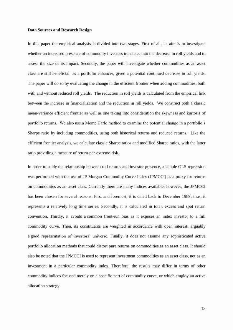
indices7. Roll yields are regressed against several variables. First, a hedging pressure variable was

considered and the following formula was implemented to describe it:

, (4)

where hp denotes hedging pressure and CSt and CLt are consecutive quantities of commercial long and

short positions in month t. The source of this data is from the US Commodity Futures Trading

Commission (CFTC) , and the traditional CFTC classification of traders into the following categories:

commercial, non-commercial, spread and unclassified was used. Only futures positions (excluding

options, swaps, etc.) were taken into account. Since roll yields were calculated on the basis of the

entire commodity index, the hedging pressure was also calculated as a sum of traders’ positions in

several markets, including cocoa, coffee, copper, corn, crude oil, gold, heating oil, lean hogs, live

cattle, natural gas, platinum, RBOB gasoline, silver, soya, soybean oil sugar and wheat markets. This

approach not only represents a market-wide perspective on the level of hedging pressure, but also

matches roughly the structure of hedging pressure within the structure of the JP Morgan index.

The Exhibit 1 presents the level of hp during the analyzed period. It should be noted that hedging

pressure across commodities was almost always in positive territory, which means that there were

usually more commercial short than long positions.

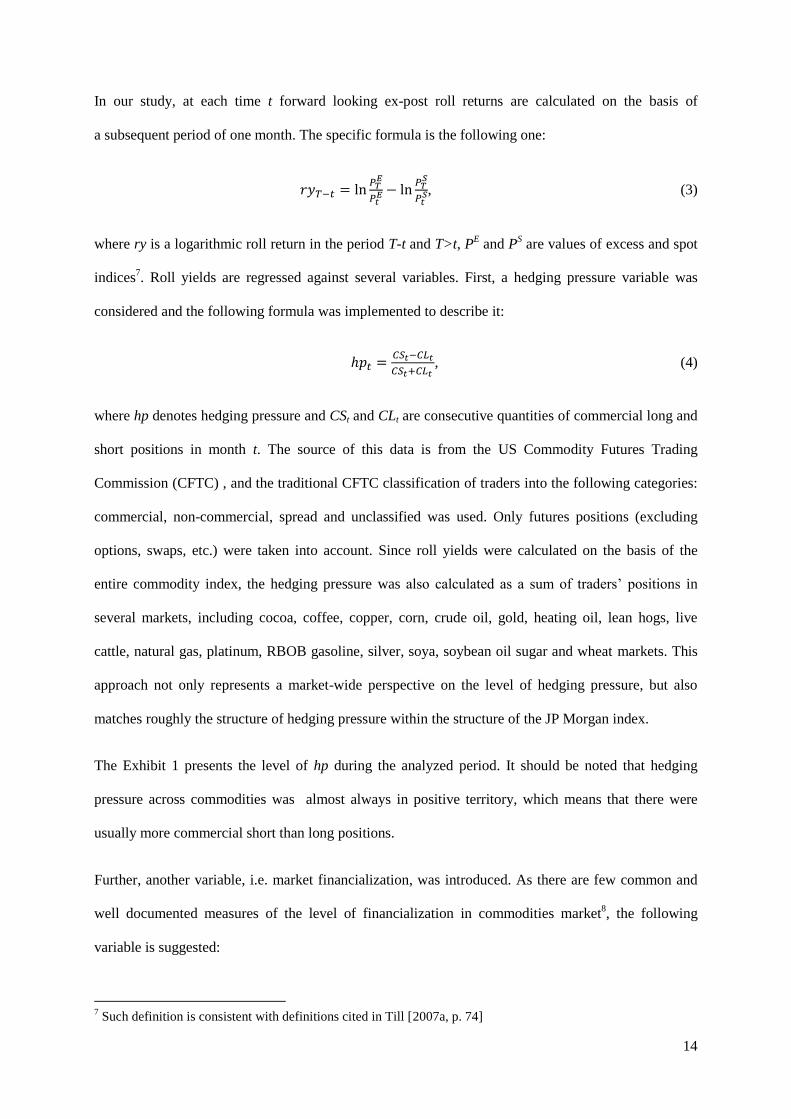
Further, another variable, i.e. market financialization, was introduced. As there are few common and

well documented measures of the level of financialization in commodities market8, the following

variable is suggested:

7 Such definition is consistent with definitions cited in Till [2007a, p. 74]

15

. (5)

In other words, the financialization variable, fin, is defined as the share of all non-commercial traders’

positions in the market (NCL – non-commercial longs, NCS – non-commercial shorts, NCSP – non-

commercial spreads) as a fraction of the total open interest. As shown in Exhibit 2, the share of non-

commercial traders in the market has systematically increased for the last 20 years at a more or less

even pace, starting from 15% in the beginning of the 1990s to over 42% at the end of 2012.

Exhibit 1. The hedging pressure in the commodity markets.

The hedging pressure was calculated as a sum of traders’ positions in commodity markets, including cocoa, coffee, copper,

corn, crude oil, gold, heating oil, lean hogs, live cattle, natural gas, platinum, RBOB gasoline, silver, soya, soybean oil sugar,

and wheat, according to the following equation,

, where hp denotes hedging pressure and CSt and CLt are

consecutively quantities of commercial long and short positions in month t. The data collected by the US Commodity Futures

Trading Commission were used.

Some studies indicate also other factors that may affect roll yield and a slope of the term structure9.

Therefore, several control variables, already mentioned in the previous literature, were introduced, as

discussed below. Nevertheless, none of these control variables actually made much difference for the

final results.

8 One exception is a measure called “speculative T-index” ascribed to Working [1960], which was recently

employed by for example Sanders, Irwin and Merrin [2008], Alquist and Gervais [2011] or Irwin and Sanders

[2010]. However, the intention of this paper is to isolate both effects connected with financialization and hedging

pressure separately, so two individual measures are used. 9 A nice review is offered by Vdovenko [2013].

-15%

-10%

-5%

0%

5%

10%

15%

20%

25%

1990 1991 1993 1994 1996 1997 1999 2000 2002 2003 2005 2006 2008 2009 2011 2012

16

Exhibit 2. The financialization level in the commodity markets.

The financialization variable was computed according to the following equation,

, where fin

denotes the level of financialization and NCLt NCSt, NCSPt and are consecutively quantities of non-commercial long, short

and spread positions in month t, and OIt represents the number of open interest. The data collected by the US Commodity

Futures Trading Commission were used.

Hong and Yogo [2012] provided theoretical and empirical evidence, according to which open interest

reveals some important information on future economic activity or inflation that cannot be attributed

to futures prices or supply and demand imbalances. The authors theorize that the amount of open

positions may be procyclical as producers and consumers take additional positions in anticipation of

higher demand. Hong and Yoko indicated that an average growth rate of an open interest is positively

correlated with market excess returns. The concept developed by the abovementioned researchers is

consistent with the hypothesis of Sockin and Xiong [2012], who believe that open interest increases

with the expectations of higher demand among commodity consumers. To sum up, it is plausible to

assume that there might be some positive correlation between the past growth of open interest and

future roll yields. Thus, open interest dynamics variable, oid, was added as a variable:

(

), (6)

The oid variable is defined as the monthly logarithmic growth of open interest OI.

0%

5%

10%

15%

20%

25%

30%

35%

40%

45%

1990 1991 1993 1994 1996 1997 1999 2000 2002 2003 2005 2006 2008 2009 2011 2012

17

Some papers [Frankel 2006, Fama and French 1988, Hong and Yogo 2009] documented the

relationship between interest rates and the term structure that results from various economic forces.

Thus, an int variable, represented by a one-month BBA USD LIBOR level, was introduced.

Bailey and Chan [1993] examine the impact of corporate spread on the futures basis. According to

them, such corporate spread may represent “a systematic risk of an underlying commodity”

[Vdovenko 2013]. Bailey and Chan [1993] interpret the relation of the corporate spread and the futures

basis from the perspective of equilibrium asset-pricing theories. They use the corporate spread as

a popular reflection of the systematic risks in the economy, which should be compensated with the risk

premium. If the roll yields are key component of the risk premiums, than variation in premiums for

systematic risks can cause common variability in the roll yields. As suggested by Acharya et al.

[2013], the term yield involves some information on default risk as it could incline producers to hedge

more in a risky environment. Producers may be prone to hedge more if the perceived risk of default is

high. To summarize, there might be present some correlation between present credit risk and future

returns. Although the influence of this phenomenon might have already been included within the

hedging pressure variable, the US corporate BAA spread, calculated over a 10-year yield (baa), was

implemented as a control variable.

Hong and Yogo in their paper of 2009 also implied that market volatility might also drive the term

structure of the commodity futures. They analyzed the VIX index of implied option volatility. Despite

the fact that the correlation observed by Hong and Yogo was of no statistical significance, the VIX

was used as a control variable, because some papers suggest, that the VIX level may influence the

expected returns in commodity markets [Munenzon 2012].

Finally, there are many studies exploring the positive relation to economic activity [Adams et al. 2008,

Armstead and Venkatraman 2007, Gorton and Rouwenhorst 2006, Kat and Oomen 2007a, Kat and

Oomen 2007b, Strongin and Petch 1995, Strongin and Petch 1996]. Economic intuition may suggest

that the state of economy could also exert some impact on the commodity futures term structure.

A high pace of economic growth may induce bigger demand for commodities and, therefore, “push

18

up” spot prices related to medium- and long-term futures. In fact, spot prices may increase even as

a result of a pure anticipation of economic improvement. In other words, the better the shape of the

economy, the lower the future roll yields. This concept appears to correspond with Hamilton

observations [2011], according to which 10 out of 11 recessions were preceded by a substantial surge

of spot prices. On the other hand, Dempster et al. [2012] indicated a positive correlation between

convenience yields and the term structure in bonds market perceived by them as a proxy for incoming

recession10

. In other words, when the tem structure in bonds market is downward sloping, this is a sign

of a final wave of growth of the economy and that a recession is ahead. This, in turn, translates into

lower expected roll yields. Thus, to estimate the relationship to present and future economy

conditions, two additional control variables representing the present and anticipated state of the

economy were introduced, i.e. the US ISM Manufacturing Index (ism) and the US government bond

term structure (term), calculated as the difference between the YTMs of 10-year and 2-year benchmark

bonds.

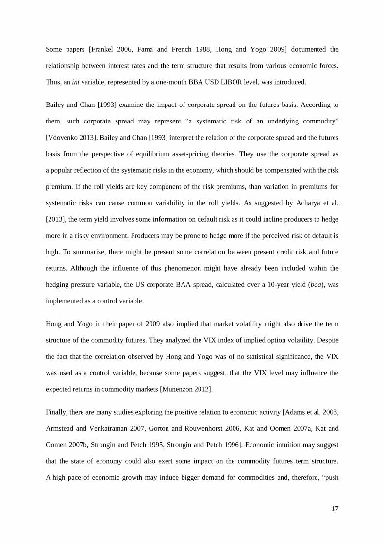
Table 1 summarizes all the explanatory variables included in the research and their expected impact on

future roll yields. Tables 2 and 3 present the basic statistical characteristics of all regression inputs and

the correlation matrix between variables.

Table 1. The explanatory variables included in the regression analysis.

The table below lists the explanatory variables employed in the regression analysis and their expected impact on the roll

returns.

Variable Notation Expected impact on future roll returns

Corporate spread baa positive

Financialisation fin negative

Hedging pressure hp positive

Interest rates int positive

Market volatility vix positive

Open interest dynamics oid negative

Recession term positive

State of the economy ism negative

10

There is a popular interpretation of the yield curve spread as a proxy for recession [Estrella and Mishkin

1998].

19

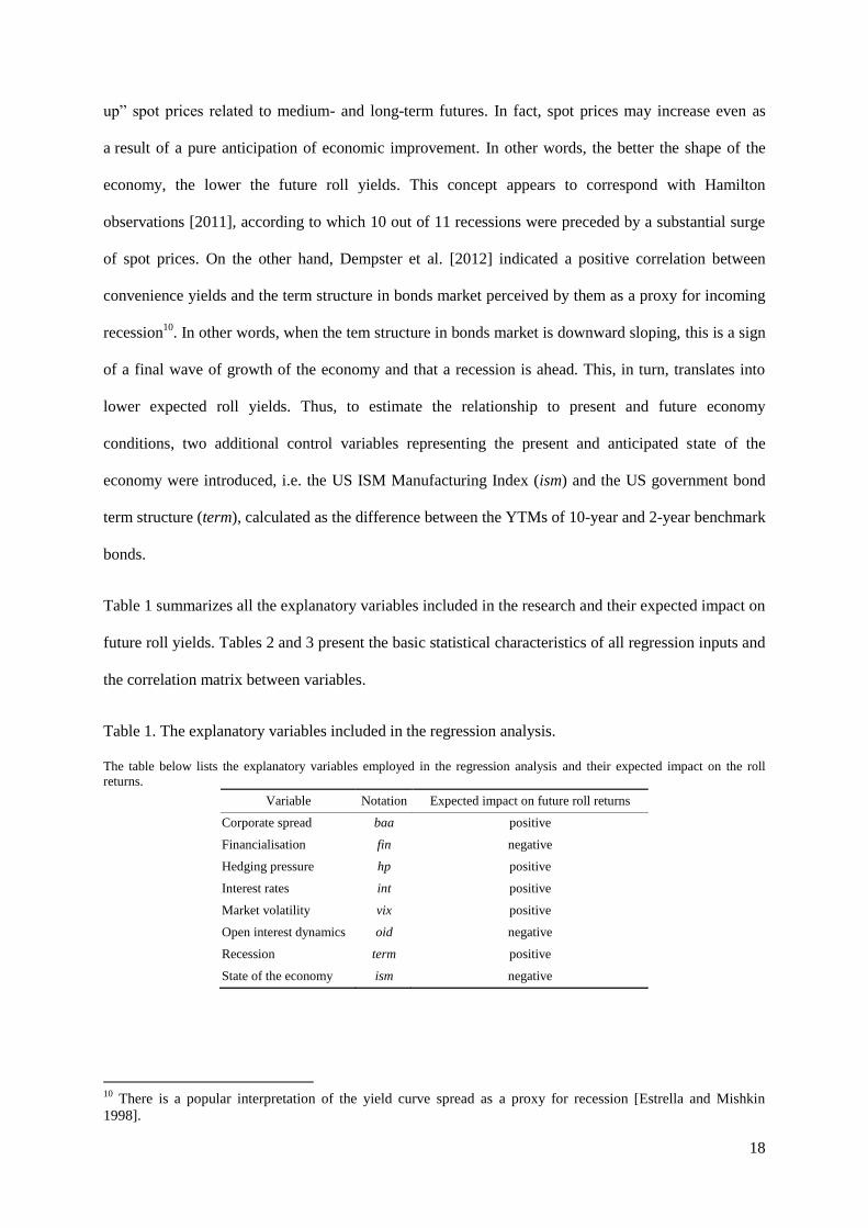
Table 2. Basic characteristics of the variables included in the regression.

The table presents the basic statistical characteristics of the independent and the dependent variable. The monthly

observations are used. The first variable is the dependent variable which is the time series of the 1-month roll returns. The

next variables are independent and described according to the notation in the Table 1. The data come from the CFTC and

Bloomberg.

ry1m baa fin hp ism int oid vix term

Average -0,001 234,461 0,252 0,082 51,640 3,708 0,007 20,439 1,163

Standard deviation 0,006 81,767 0,091 0,055 5,155 2,315 0,042 7,779 0,919

Skewness 0,413 1,751 0,295 -0,272 -0,819 -0,131 1,357 1,583 0,092

Kurtosis 1,692 4,608 -1,425 -0,110 0,949 -1,097 9,624 4,009 -1,364

Number of observations 275 275 275 275 275 275 275 275 275

Table 3. Correlations between the explanatory variables.

The table presents the correlations between the explanatory variables employed. The computations are based on monthly

observations and the data come from the CFTC and Bloomberg. The notation of the variables is presented in the Table 1.

fin hp term vix oid rf baa ism

fin 1,00

hp 0,05 1,00

term 0,26 0,28 1,00

vix 0,22 -0,26 0,17 1,00

oid 0,02 0,05 -0,03 -0,14 1,00

rf -0,65 -0,19 -0,80 -0,18 -0,03 1,00

baa 0,52 -0,11 0,51 0,72 -0,13 -0,62 1,00

ism 0,10 0,37 0,07 -0,45 0,17 -0,18 -0,47 1,00

All the data comes from Bloomberg and the CFTC website. Time-series are computed on a monthly

basis, consistent with the analyses performed later in the paper. Thus, the initial regression was also

performed on the basis of monthly data. The second research stage comprises two analyses. The first

one was based on historical data and essentially examines the historical relationship between

financialization and roll yields. We assume the detected relationship is one of causality. We also

assume that the detected impact of financialization from the first regression will continue into the

future, and so the second set of studies simulates the portfolio properties of commodities using lower

returns than historical returns. Further details on our analyses are provided below.

The mean-variance spanning test is designed to verify whether inclusion of an asset class in a portfolio

results in the expansion of investor’s efficient frontier. The test was initially proposed by Huberman

and Kendel [1987], and later developed by Ferson et al. [1993], De Santis [1993] and Bekaert and

20

Urias [1996]. In addition, Jobson and Korkie [1988] as well as Chen and Knez [1996], showed that

such a test could be used in order to assess investment performance. De Roon and Nijman [2001]

proved that it might be used in terms of non-marketable assets11

. Finally, it should be noted that many

examples of mean-variance spanning tests performed with respect to commodities are also available.

The mean-variance spanning test examines whether investor’s efficient frontier is significantly

augmented due to inclusion of a new asset class. If a risk-free asset is available, it is sufficient to

examine the shift of the tangency portfolio [Kan and Zhou 2012]. If the tangency portfolio is moved,

an investor is able to build better optimal portfolios composed of a risk-free asset and a tangency

portfolio. It is worth noticing that the improvement in a tangency portfolio equals, in fact, the

improvement in the Sharpe ratio.

In what follows, we examine whether the inclusion of commodities expands the efficient frontier of

a traditional portfolio comprising stocks and bonds. The test is made from perspective of the US

investor, comprising dollar denominated assets. The equities as an asset class are represented by

Wilshire 5000 Total Market, and the proxy for the US government bonds is Bloomberg/EFFAS US

Government Bonds All 1+. Once again, the JP Morgan Commodity Curve Index is used as the

commodity portfolio. All the indices are calculated in a total return regime. Additionally, USD BBA

one-month Libor is used in order to calculate excess returns on risk-free assets. All the data comes

from Bloomberg and comprises the period between December 31, 1991 and December 31, 2012. Thus,

all three indices are calculated from the very beginning. Arithmetical rates of return are computed on

a monthly basis.

In this paper the mean-variance spanning is tested in two ways: using traditional OLS regression and

with the use of Monte Carlo analysis. The second method is based on two distinct risk measures. The

details of both methods are described below.

The majority of mean-variance spanning tests are based on total rates of return. Therefore, it is

plausible to assume that exposure to various asset classes should sum up to 1. However, in this

11

A nice review of mean-variance spanning tests can be found in the paper of De Roon and Nijman [2001].

21

research, risk premiums defined as excess returns on financial market were used. In the regression

tests, the approach of Scherer and He [2008, p. 246] is used. The regression model shall be as follows:

it

K

k

tktikitit cRcR 1

)(

, (7)

where Rit is the return on the examined asset class (commodities), ct denotes financial market return in

month t, and Rkt is k-asset’s rate of return (stocks and bonds). If , as specified in the model above,

turns out to be statistically different from and higher than 0, one can say, that i constitutes a distinct

asset class that generates its own risk premium. However, if this statement does not hold true, an

investor can probably replicate i’s returns without bearing higher risk or losing some of their returns.

This method is consistent with remarks of Anson [2009], and was used in respect to commodity

market e.g. by Nijman and Swinkels [2008]. The risk premium approach appears to be reasonable for

at least three reasons. Firstly, it does not imply that the betas need to sum up to 1. Missing allocation

can be filled with cash or negative cash in the case of leverage. Secondly, it facilitates the graphical

interpretation and further analysis as the tangency line of the tangency portfolio is drawn from the

origins of the coordinate system. Finally, it seems more practical as it corresponds with futures

contracts employed in order to obtain exposure to particular asset classes.

The main issue with the traditional OLS regression in the case of commodities is that the return

distribution of commodities seems to be far from normal [Anson 2009, Gorton and Rouwenhorst 2006,

Erb and Harvey 2006]. In consequence, the standard deviation might underestimate the true level of

investor risk due to skewed distributions and fat tails, if an investor has skewness and kurtosis

preferences. The problem is further explored by Johaning et al. [2006]. According to some studies in

this field, it is recommended to take into account also higher moments in the process of portfolio

analysis [Arditti and Levy 1975, Markowitz 1952, Samuelson 1970, Harvey, Liechty, Liechty

and Muller 2004, Cvitanic 2008, Fang and Lai 1997, Dittmar 2002].

22

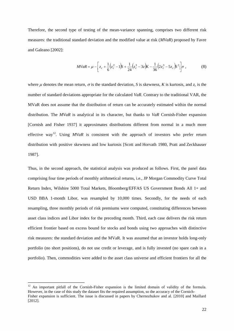
Therefore, the second type of testing of the mean-variance spanning, comprises two different risk

measures: the traditional standard deviation and the modified value at risk (MVaR) proposed by Favre

and Galeano [2002]:

2332 52

36

13

24

11

6

1SzzKzzSzzMVaR ccccc , (8)

where denotes the mean return, is the standard deviation, S is skewness, K is kurtosis, and zc is the

number of standard deviations appropriate for the calculated VaR. Contrary to the traditional VAR, the

MVaR does not assume that the distribution of return can be accurately estimated within the normal

distribution. The MVaR is analytical in its character, but thanks to VaR Cornish-Fisher expansion

[Cornish and Fisher 1937] it approximates distributions different from normal in a much more

effective way12

. Using MVaR is consistent with the approach of investors who prefer return

distribution with positive skewness and low kurtosis [Scott and Horvath 1980, Pratt and Zeckhauser

1987].

Thus, in the second approach, the statistical analysis was produced as follows. First, the panel data

comprising four time periods of monthly arithmetical returns, i.e., JP Morgan Commodity Curve Total

Return Index, Wilshire 5000 Total Markets, Bloomberg/EFFAS US Government Bonds All 1+ and

USD BBA 1-month Libor, was resampled by 10,000 times. Secondly, for the needs of each

resampling, three monthly periods of risk premiums were computed, constituting differences between

asset class indices and Libor index for the preceding month. Third, each case delivers the risk return

efficient frontier based on excess bound for stocks and bonds using two approaches with distinctive

risk measures: the standard deviation and the MVaR. It was assumed that an investor holds long-only

portfolio (no short positions), do not use credit or leverage, and is fully invested (no spare cash in a

portfolio). Then, commodities were added to the asset class universe and efficient frontiers for all the

12

An important pitfall of the Cornish-Fisher expansion is the limited domain of validity of the formula.

However, in the case of this study the dataset fits the required assumption, so the accuracy of the Cornich-

Fisher expansion is sufficient. The issue is discussed in papers by Chernozhukov and al. [2010] and Maillard

[2012].

23

three asset classes were explored. Further, Sharpe ratios for tangency portfolios13

for both efficient

frontiers were calculated in both cases (four ratios in total). It should also be noted that, in terms of

the MVaR, the measure is, in fact, dubbed as the modified Sharpe ratio described by Bacon [2008, p.

102]. Subsequently, the improvement in Sharpe ratios was computed due to the difference between the

values after and prior to the commodity inclusion. As has already been noted, in the case of the excess

return framework (or in other words: risk premium framework), the improvement in the maximum

achievable Sharpe ratio is, in fact, equal to the mean-variance intersection. Next, the percentage of

resampled efficient frontiers (percentage out of 10,000) was calculated and it involved Sharpe ratio’s

improvement. The percentage of cases in which the Sharpe ratios did not increase shall be my p-value.

One of the benefits of the resampling approach described above is that it does not require any special

assumptions regarding the underlying distribution of return. However, its disadvantage is that it does

not take into consideration the path-dependency of data.

In a nutshell, the whole analysis described above was conducted twice: first, with no consideration of

any decrease in roll yields, and secondly, after simulating a decrease in roll yields due to

financialization. The size of this decline was derived from the regression analysis performed at the

earlier stage of this research.

Results and Interpretation

Table 4 presents the results of regression analysis of monthly roll returns against the variables

described in the earlier part of this paper. The regression was performed in a few configurations;

however, in any case only financialization and hedging pressure are statistically significant at the level

of 5%. In fact, the level of the significance of financialization is the strongest of all the variables.

Additionally, the corporate spread is also significant at the level of 5% in one of the regressions;

however, contrary to the underlying theory, the sign of a corresponding parameter is negative.

Therefore, this parameter was not used in the further stage of the analysis. The regression, which

comprises the highest number of parameters with significance at min. 1%, includes only two variables:

financialization and hedging pressure (see: Formula (1) in the Table 4). This regression bears also the

13

The tangency portfolios are characterised in this case by the maximum attainable Sharpe ratios.

24

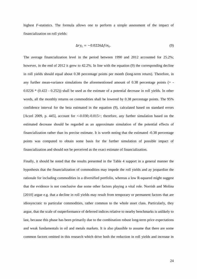
highest F-statistics. The formula allows one to perform a simple assessment of the impact of

financialization on roll yields:

. (9)

The average financialization level in the period between 1990 and 2012 accounted for 25.2%;

however, in the end of 2012 it grew to 42.2%. In line with the equation (9) the corresponding decline

in roll yields should equal about 0.38 percentage points per month (long-term return). Therefore, in

any further mean-variance simulations the aforementioned amount of 0.38 percentage points (= -

0.0226 * (0.422 - 0.252)) shall be used as the estimate of a potential decrease in roll yields. In other

words, all the monthly returns on commodities shall be lowered by 0.38 percentage points. The 95%

confidence interval for the beta estimated in the equation (9), calculated based on standard errors

[Aczel 2009, p. 445], account for <-0.030;-0.015>; therefore, any further simulation based on the

estimated decrease should be regarded as an approximate simulation of the potential effects of

financialization rather than its precise estimate. It is worth noting that the estimated -0.38 percentage

points was computed to obtain some basis for the further simulation of possible impact of

financialization and should not be perceived as the exact estimate of financialization.

Finally, it should be noted that the results presented in the Table 4 support in a general manner the

hypothesis that the financialization of commodities may impede the roll yields and ay jeopardize the

rationale for including commodities in a diversified portfolio, whereas a low R-squared might suggest

that the evidence is not conclusive due some other factors playing a vital role. Norrish and Molina

[2010] argue e.g. that a decline in roll yields may result from temporary or permanent factors that are

idiosyncratic to particular commodities, rather common to the whole asset class. Particularly, they

argue, that the scale of outperformance of deferred indices relative to nearby benchmarks is unlikely to

last, because this phase has been primarily due to the combination robust long-term price expectations

and weak fundamentals in oil and metals markets. It is also plausible to assume that there are some

common factors omitted in this research which drive both the reduction in roll yields and increase in

25

non-commercial open interest. These issues shall be investigated in a more precise and detailed way in

further research.

Table 4. The impact of the explanatory variables on the roll return.

The regression model estimated for the roll returns of the JP Morgan Commodity Curve Index is based on monthly

observations. We run eight distinct multivariate regressions with various combinations of explanatory variables. The

variables are named according to the notation in Table 1. The first number in each cell is the OLS estimation of the

coefficient for the corresponded variable. A number in brackets is the t-statistics. “N” is the number of observations. The

symbols *, **, and *** denote the statistical significance at the 10%, 5% and 1% levels. The data come from the CFTC and

Bloomberg.

(1) (2) (3) (4) (5) (6) (7) (8)

intercept 0,003*** 0,003*** 0,004*** 0,003*** 0,004 0,004*** 0,000 0,017*

-2,67 (2,75) (2,74) (2,70) (1,09) (3,34) (0,09) (1,85)

baa 0,000** 0,000**

(-2,01) (-2,24)

fin -0,023*** -0,021*** -0,022*** -0,023*** -0,022*** -0,018*** -0,017*** -0,012*

(-5,79) (-5,28) (-5,37) (-5,78) (-5,74) (-3,86) (-3,31) (-1,83)

hp 0,019*** 0,021*** 0,017** 0,019*** 0,02*** 0,017** 0,021*** 0,021***

(2,91) (3,16) (2,52) (2,97) (2,80) (2,56) (3,2) (2,86)

ism 0,000 0,000*

(-0,29) -1,818

oid -0,011 -0,012

(-1,28) (-1,46)

rf 0,000*** 0,000

(1,66) (-0,25)

term -0,001 0,000

(-1,29) (0,28)

vix 0,000 0,000

(-1,03) (0,77)

N 275 275 275 275 275 275 275 275

adj. R2 0,123 0,125 0,123 0,125 0,12 0,133 0,129 0,138

F-stat 20,185 14,04 13,814 14,031 13,439 14,956 14,469 6,481

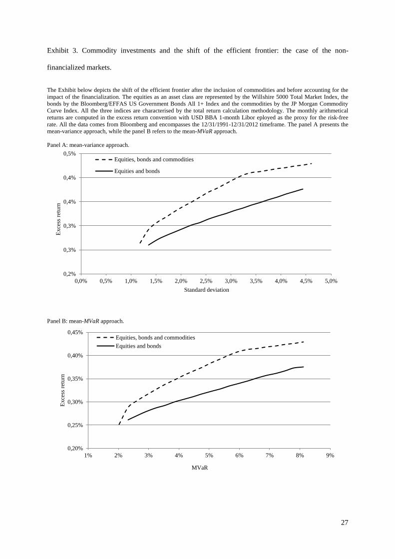
Exhibit 3 depicts the expansion of the efficient frontier as a result of inclusion of commodities, based

on raw historical data (without calculating any impact of financialization). The efficient frontiers are

“pushed” upward and leftward after the inclusion of commodities both in the mean-variance approach

and in the mean-MVar approach.

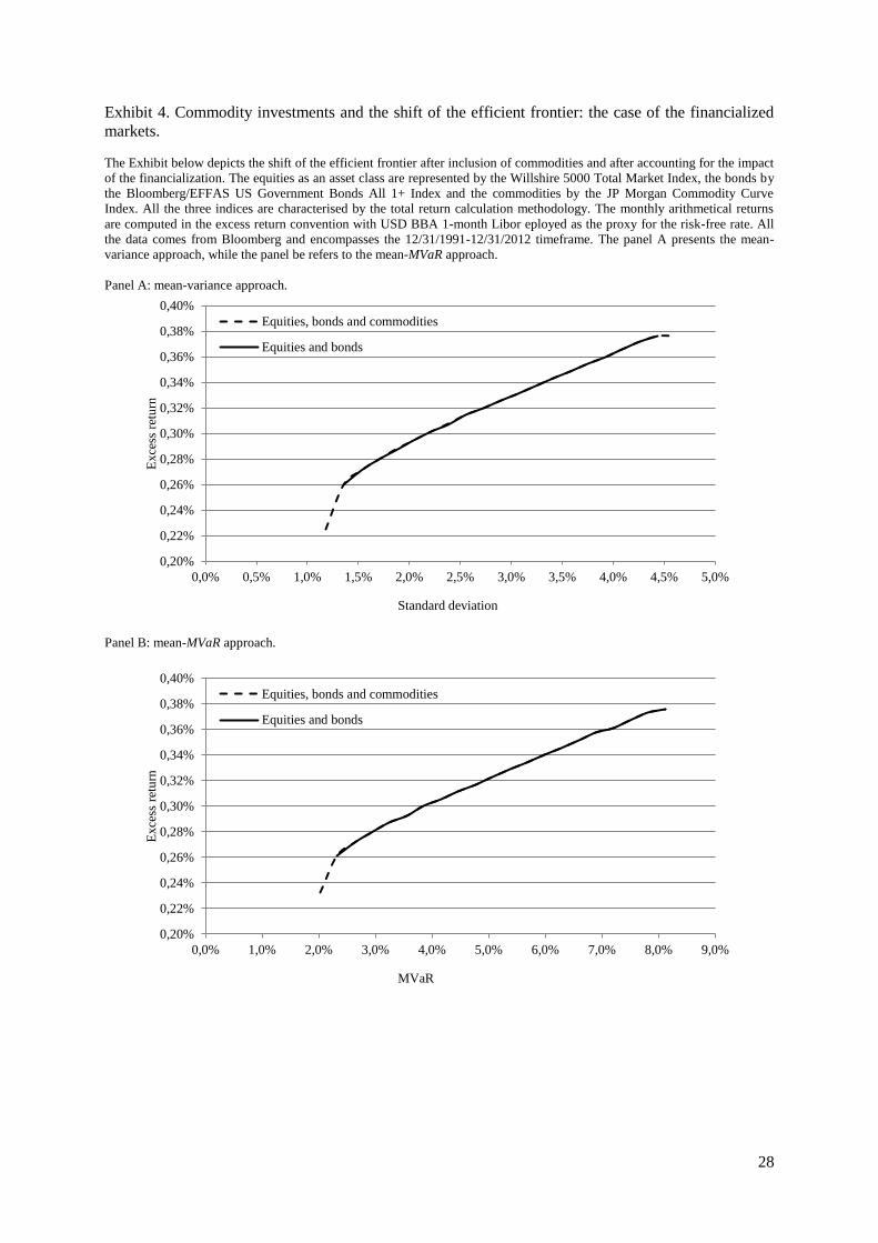
However, this conclusion does not hold true after calculation of the impact of financialization. As it

follows from the Exhibit 4, none of the bounds offer better investment opportunities. Table 5 presents

the results of mean variance spanning test analysis using the regression approach described in the

26

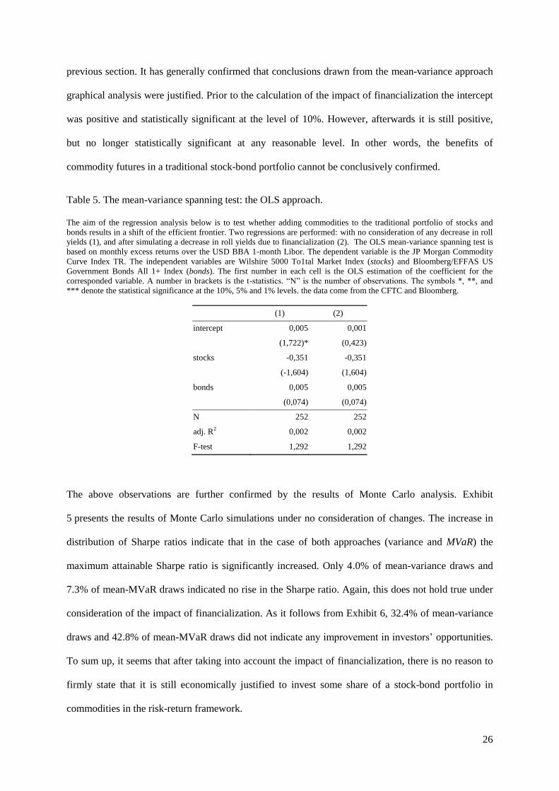
previous section. It has generally confirmed that conclusions drawn from the mean-variance approach

graphical analysis were justified. Prior to the calculation of the impact of financialization the intercept

was positive and statistically significant at the level of 10%. However, afterwards it is still positive,

but no longer statistically significant at any reasonable level. In other words, the benefits of

commodity futures in a traditional stock-bond portfolio cannot be conclusively confirmed.

Table 5. The mean-variance spanning test: the OLS approach.

The aim of the regression analysis below is to test whether adding commodities to the traditional portfolio of stocks and

bonds results in a shift of the efficient frontier. Two regressions are performed: with no consideration of any decrease in roll

yields (1), and after simulating a decrease in roll yields due to financialization (2). The OLS mean-variance spanning test is

based on monthly excess returns over the USD BBA 1-month Libor. The dependent variable is the JP Morgan Commodity

Curve Index TR. The independent variables are Wilshire 5000 To1tal Market Index (stocks) and Bloomberg/EFFAS US

Government Bonds All 1+ Index (bonds). The first number in each cell is the OLS estimation of the coefficient for the

corresponded variable. A number in brackets is the t-statistics. “N” is the number of observations. The symbols *, **, and

*** denote the statistical significance at the 10%, 5% and 1% levels. the data come from the CFTC and Bloomberg.

(1) (2)

intercept 0,005 0,001

(1,722)* (0,423)

stocks -0,351 -0,351

(-1,604) (1,604)

bonds 0,005 0,005

(0,074) (0,074)

N 252 252

adj. R2 0,002 0,002

F-test 1,292 1,292

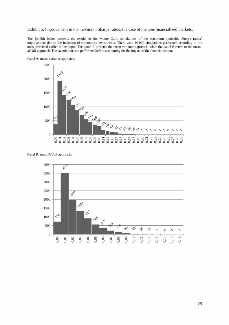
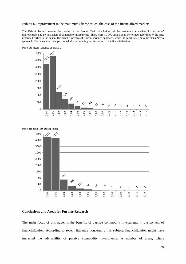
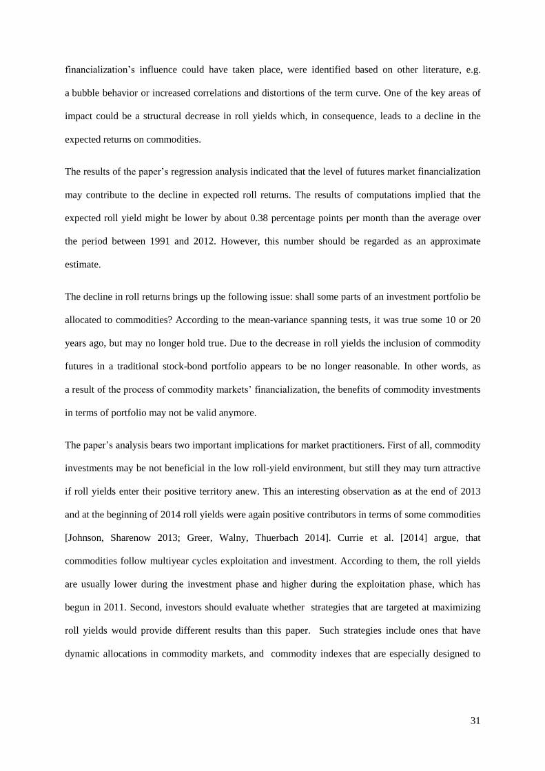
The above observations are further confirmed by the results of Monte Carlo analysis. Exhibit

5 presents the results of Monte Carlo simulations under no consideration of changes. The increase in

distribution of Sharpe ratios indicate that in the case of both approaches (variance and MVaR) the

maximum attainable Sharpe ratio is significantly increased. Only 4.0% of mean-variance draws and

7.3% of mean-MVaR draws indicated no rise in the Sharpe ratio. Again, this does not hold true under

consideration of the impact of financialization. As it follows from Exhibit 6, 32.4% of mean-variance

draws and 42.8% of mean-MVaR draws did not indicate any improvement in investors’ opportunities.

To sum up, it seems that after taking into account the impact of financialization, there is no reason to

firmly state that it is still economically justified to invest some share of a stock-bond portfolio in

commodities in the risk-return framework.

27

Exhibit 3. Commodity investments and the shift of the efficient frontier: the case of the non-

financialized markets.

The Exhibit below depicts the shift of the efficient frontier after the inclusion of commodities and before accounting for the

impact of the financialization. The equities as an asset class are represented by the Willshire 5000 Total Market Index, the

bonds by the Bloomberg/EFFAS US Government Bonds All 1+ Index and the commodities by the JP Morgan Commodity

Curve Index. All the three indices are characterised by the total return calculation methodology. The monthly arithmetical

returns are computed in the excess return convention with USD BBA 1-month Libor eployed as the proxy for the risk-free

rate. All the data comes from Bloomberg and encompasses the 12/31/1991-12/31/2012 timeframe. The panel A presents the

mean-variance approach, while the panel B refers to the mean-MVaR approach.

Panel A: mean-variance approach.

Panel B: mean-MVaR approach.

0,2%

0,3%

0,3%

0,4%

0,4%

0,5%

0,0% 0,5% 1,0% 1,5% 2,0% 2,5% 3,0% 3,5% 4,0% 4,5% 5,0%

Exce

ss r

etu

rn

Standard deviation

Equities, bonds and commodities

Equities and bonds

0,20%

0,25%

0,30%

0,35%

0,40%

0,45%

1% 2% 3% 4% 5% 6% 7% 8% 9%

Exce

ss r

etu

rn

MVaR

Equities, bonds and commodities

Equities and bonds

28

Exhibit 4. Commodity investments and the shift of the efficient frontier: the case of the financialized

markets.

The Exhibit below depicts the shift of the efficient frontier after inclusion of commodities and after accounting for the impact

of the financialization. The equities as an asset class are represented by the Willshire 5000 Total Market Index, the bonds by

the Bloomberg/EFFAS US Government Bonds All 1+ Index and the commodities by the JP Morgan Commodity Curve

Index. All the three indices are characterised by the total return calculation methodology. The monthly arithmetical returns

are computed in the excess return convention with USD BBA 1-month Libor eployed as the proxy for the risk-free rate. All

the data comes from Bloomberg and encompasses the 12/31/1991-12/31/2012 timeframe. The panel A presents the mean-

variance approach, while the panel be refers to the mean-MVaR approach.

Panel A: mean-variance approach.

Panel B: mean-MVaR approach.

0,20%

0,22%

0,24%

0,26%

0,28%

0,30%

0,32%

0,34%

0,36%

0,38%

0,40%

0,0% 0,5% 1,0% 1,5% 2,0% 2,5% 3,0% 3,5% 4,0% 4,5% 5,0%

Exce

ss r

etu

rn

Standard deviation

Equities, bonds and commodities

Equities and bonds

0,20%

0,22%

0,24%

0,26%

0,28%

0,30%

0,32%

0,34%

0,36%

0,38%

0,40%

0,0% 1,0% 2,0% 3,0% 4,0% 5,0% 6,0% 7,0% 8,0% 9,0%

Exce

ss r

etu

rn

MVaR

Equities, bonds and commodities

Equities and bonds

29

Exhibit 5. Improvement in the maximum Sharpe ratios: the case of the non-financialized markets.

The Exhibit below presents the results of the Monte Carlo simulations of the maximum attainable Sharpe ratios’

improvement due to the inclusion of commodity investments. There were 10 000 simulations performed according to the

ones described earlier in the paper. The panel A presents the mean-variance approach, while the panel B refers to the mean-

MVaR approach. The calculations are performed before accounting for the impact of the financialization.

Panel A: mean-variance approach.

Panel B: mean-MVaR approach.

0

500

1000

1500

2000

2500

0,0

0

0,0

1

0,0

2

0,0

3

0,0

4

0,0

5

0,0

6

0,0

7

0,0

8

0,0

9

0,1

0

0,1

1

0,1

2

0,1

3

0,1

4

0,1

5

0,1

6

0,1

7

0,1

8

0,1

9

0,2

0

0,2

1

0,2

2

0,2

3

0,2

4

0,2

5

0,2

6

0,2

7

0,2

8

0,2

9

0

500

1000

1500

2000

2500

3000

3500

4000

0,0

0

0,0

1

0,0

2

0,0

3

0,0

4

0,0

5

0,0

6

0,0

7

0,0

8

0,0

9

0,1

0

0,1

1

0,1

2

0,1

3

0,1

4

0,1

5

0,1

6

30

Exhibit 6. Improvement in the maximum Sharpe ratios: the case of the financialized markets.

The Exhibit below presents the results of the Monte Carlo simulations of the maximum attainable Sharpe ratios’

improvement due the inclusion of commodity investments. There were 10 000 simulations performed according to the ones

described earlier in the paper. The panel A presents the mean-variance approach, while the panel B refers to the mean-MVaR

approach. The calculations are performed after accounting for the impact of the financialization.

Panel A: mean-variance approach.

Panel B: mean-MVaR approach.

Conclusions and Areas for Further Research

The main focus of this paper is the benefits of passive commodity investments in the context of

financialization. According to recent literature concerning this subject, financialization might have

impacted the advisability of passive commodity investments. A number of areas, where

0

500

1000

1500

2000

2500

3000

3500

4000

0,0

0

0,0

1

0,0

2

0,0

3

0,0

4

0,0

5

0,0

6

0,0

7

0,0

8

0,0

9

0,1

0

0,1

1

0,1

2

0,1

3

0,1

4

0,1

5

0,1

6

0

500

1000

1500

2000

2500

3000

3500

4000

4500

0,0

0

0,0

1

0,0

2

0,0

3

0,0

4

0,0

5

0,0

6

0,0

7

0,0

8

0,0

9

0,1

0

0,1

1

0,1

2

31

financialization’s influence could have taken place, were identified based on other literature, e.g.

a bubble behavior or increased correlations and distortions of the term curve. One of the key areas of

impact could be a structural decrease in roll yields which, in consequence, leads to a decline in the

expected returns on commodities.

The results of the paper’s regression analysis indicated that the level of futures market financialization

may contribute to the decline in expected roll returns. The results of computations implied that the

expected roll yield might be lower by about 0.38 percentage points per month than the average over

the period between 1991 and 2012. However, this number should be regarded as an approximate

estimate.

The decline in roll returns brings up the following issue: shall some parts of an investment portfolio be

allocated to commodities? According to the mean-variance spanning tests, it was true some 10 or 20

years ago, but may no longer hold true. Due to the decrease in roll yields the inclusion of commodity

futures in a traditional stock-bond portfolio appears to be no longer reasonable. In other words, as

a result of the process of commodity markets’ financialization, the benefits of commodity investments

in terms of portfolio may not be valid anymore.

The paper’s analysis bears two important implications for market practitioners. First of all, commodity

investments may be not beneficial in the low roll-yield environment, but still they may turn attractive

if roll yields enter their positive territory anew. This an interesting observation as at the end of 2013

and at the beginning of 2014 roll yields were again positive contributors in terms of some commodities

[Johnson, Sharenow 2013; Greer, Walny, Thuerbach 2014]. Currie et al. [2014] argue, that

commodities follow multiyear cycles exploitation and investment. According to them, the roll yields

are usually lower during the investment phase and higher during the exploitation phase, which has

begun in 2011. Second, investors should evaluate whether strategies that are targeted at maximizing

roll yields would provide different results than this paper. Such strategies include ones that have

dynamic allocations in commodity markets, and commodity indexes that are especially designed to

32

maximize roll yields. Such issues are further discussed e.g. by Campbell & Company [2014] and by

Greer et al. [2012].

Any further research shall focus on several issues. First of all, it would be interesting to test the

correlation between financialization and roll yields and its impact on the benefits of commodity

investing at the level of single commodities. Secondly, it would be valuable to identify and include

some other factors that may influence roll yields and open interest in the research, with the aim to

assess the impact of financialization in a much more precise way. Then, from perspective of

practitioners, it would be useful to explore the extent to which employing some specific commodity

indices or pursuing active strategies may mitigate the negative impact of financialization. Finally, also

the impact of other phenomena related to financialization, such as e.g. changes in interdependencies

between returns of various asset classes, should be explored.

References

Abanomey W.S., I. Mathur. “Intercontinental Portfolios with Commodity Futures and Currency

Forward Contracts.” Journal of Investing, autumn (2001), pp. 61–68.

Acharya V.V., L. A. Lochstoer, T. Ramadoraie. “Limits to arbitrage and hedging: Evidence from

commodity markets.” Journal of Financial Economics, Vol. 109, No. 2 (2013), pp. 441–465.

Aczel A.D., J. Sounderpandian. “Complete business statistics”. Boston: McGraw-Hill/Irwin, 2009.

Adams Z., R. Füss, D.G. Kaiser. “Macroeconomic Determinants of Commodity Futures Returns”. In::

F.J. Fabozzi, R. Füss, D.G. Kaiser (ed.) The Handbook of Commodity Investing. John Wiley & Sons,

Hoboken, New Jersey, USA, 2008, pp. 87–112.

Akey R.P. “Alpha, Beta, and Commodities: Can a Commodities Investment be Both a High-Risk-

Ajdusted Return Source and a Portfolio Hedge?” In: H. Till, J. Eagleeye (ed.) Intelligent Commodity

Investing: New Strategies and Practical Insights for Informed Decision Makings. London: Risk Books,

2007, pp. 377–417.

33

Anderson R., J-P. Danthine. “Cross-hedging.” Journal of Political Economy, Vol. 89 (1981), pp. 1182-

1196.

Ankrim E.M., C.R. Hensel. “Commodities in Asset Allocation: A Real-Asset Alternative to Real

Estate?” Financial Analyst Journal, may/june (1993), pp. 20–29.

Anson M.J.P. “Spot Returns, Roll Yield and Diversification with Commodity Futures”. Journal of

Alternative Investments, winter (1999), pp. 1–17.

Anson M.J.P. Handbook of Alternative Investments, 2nd

issue, Hoboken: Wiley, 2006.

Arditti E.D., H. Levy. “Portfolio Efficiency Analysis in Three Moments: The Multiperiod Case”,

Journal of Finance, Vol. 30, No. 3 (1975), pp. 797–809.

Armstead K.J., R. Venkatraman.“Commodity Returns - Implications for Active Management.” In: H.

Till, J. Eagleeye (ed.), Intelligent Commodity Investing: New Strategies and Practical Insights for

Informed Decision Makings, London: Risk Books, 2007, pp. 293–312.

Aulerich N.M, Irwin S.H. & Garcia P. “Bubbles, Food Prices, and Speculation: Evidence from the

CFTC's Daily Large Trader Data Files.” NBER Working Paper No. 19065

http://www.nber.org/papers/w19065.pdf, 2013.

Authers J. The Fearful Rise of Markets. Upper Saddle River: FT Press, 2010.

Bacon C.R. Practical Portfolio Performance Measurement and Attribution. Chichester: Wiley, 2008.

Bailey W., K.C. Chan. “Macroeconomic Influences and the Variability of the Commodity Futures

Basis.” Journal of Finance, Vol. 48, No. 2 (1993), pp. 555-573

Basu D., J. Miffre. “Capturing the Risk Premium of Commodity Futures: The Role of Hedging

Pressure”, EDHEC Working Paper, 2013.

34

Becker K.G., J.E. Finnerty. “Indexed Commodity Futures and the Risk of Institutional Portfolios.”

OFOR working paper, No. 94–02, January, 1994.

Bekaert G., M.S. Urias. “Diversification, Integration and Emerging Market Closed-end Funds.”

Journal of Finance, Vol. 51, No.3 (1996), pp. 835-869.

Bekkers N., R.Q. Doeswijk, T.W. Lam. “Asset Allocation: Determining the Optimal Portfolio with

Ten Asset Classes.”The Journal of Wealth Management, Vol. 12, No. 3 (2009), pp. 61-77.

Bessembinder H., Systematic Risk, Hedging Pressure and Risk Premiums in Futures Markets, Review

of Financial Studies, Vol. 5, No. 4 (1992), pp. 637–667.

Bjornson B., C.A. Carter. “New Evidence on Agricultural Commodity Return Perfomance under

Time-Varying Risk.” American Journal of Agricultural Economics 79, No. 3 (1997), pp. 918–930.

Bodie Z. “Commodity Futures as a Hedge against Inflation.” Journal of Portfolio Management, Vol. 9,

No. 3 (1983), pp. 12–17.

Bodie Z., V.I. Rosansky “Risk and Return in Commodity Futures.” Financial Analyst Journal, Vol. 36,

No. 3 (1980), pp. 27–39.

Brennan M.J. “The Price of Convenience and the Valuation of Commodity Contingent Claims.” In: D.

Land, B. Oeksendal (ed.), Stochastic Models and Options Values, Elsevier Science Publications, 1991.

Brunetti C., D. Reiffen. “Commodity Index Trading and Hedging Costs, Division of Research &

Statistics and Monetary Affairs”. Washington D.C.: Federal Reserve Board, 2011.

Burkart D.W. “Commodities and Real-Return Strategies in the Investment Mix”, CFA Institute

Conference Proceedings Quarterly, Vol. 23, No. 4., 2006.

Buyuksahin B. “Speculation Demystified: Virtuous Volatility.” IEA Energy: The Journal of the

International Energy Agency, Vol. 3 (2012), pp. 33-34.

35

Campbell & Company “Deconstructing Futures Returns: The Role of Roll Yield”, Campbell White

Paper Series, http://www.campbell.com/_files/Deconstructing%20Futures%20Returns%20-

%20The%20Role%20of%20Roll%20Yield.pdf, 2014

Carter C.A., G.C. Rausser, A. Schmitz. “Efficient Asset Portfolios and the Theory of Normal

Backwardation.” Journal of Political Economy, Vol. 91, No. 2 (1983), pp. 319–331.

Cashin P., C.J. McDermott, A. Scott. “Booms and Slumps in World Commodity Prices.” IMF

Working Paper 99/155, 1999.

Cevik S. & Sedik T.S. “A Barrel of Oil or a Bottle of Wine: How Do Global Growth Dynamics Affect

Commodity Prices?” IMF Working Paper No. 11/1 (2011),

https://www.imf.org/external/pubs/cat/longres.cfm?sk=24547.0.

Chang E.C. “Returns to Speculators and the Theory of Normal Backwardation.” Journal of Finance,

Vol. 40, No. 1 (1985), pp. 193–208.

Chen Z., P.J. Knez. ”Portfolio Performance Measurement: Theory and Applications.” Review of

Financial Studies, Vol. 9, No. 2 (1996), pp. 511-555.

Chernozhukov V., I. Fernández-Val, A. Galichon. “Rearranging Edgeworth–Cornish–Fisher

expansions.” Economic Theory, Vol. 42, No. 2 (2010), pp. 419-435.

Chong J., J. Miffre” Conditional Risk Premia, Volatilities and Correlations in Commodity Futures

Markets.”, working Paper, 2006.

Cootner P. “Returns to Speculators: Telser Versus Keynes.” Journal of Political Economy, Vol. 62

(1960), pp. 396–404.

Cootner P. “Speculation and hedging.” Food Research Institute Studies, Vol. 7 (1967), pp. 65-105.

36

Cornish E.A., R.A. Fisher. “Moments and cumulants in the specification of distributions.” Review of

the International Statistical Institute, Vol. 5 (1937), pp. 307–320.

Cuddington J.T. “Long-Run Trends in Primary Commodity Prices: A Disaggregated Look at the

Prebish-Singer Hypothesis.” Journal of Development Economics, Vol. 39 (1992), pp. 207–227.

Currie J., M. Hinds, D. Courvalin, M. Layton, et al. “Two themes for the emergent macro recovery.”.

Goldman Sachs Commodity Research, July 28, 2014.

Cvitanic J., V. Polimenish, F. Zapaterox. “Optimal Portfolio Allocation with Higher Moments.”,

Ammals of Finance, Vol. 4, No. 1 (2008), pp. 1-28.

Daskalaki C. & Skiadopoulos G.S. “Should Investors Include Commodities in Their Portfolios After

All? New Evidence.” Journal of Banking and Finance, Vol. 35, No. 10 (2011), pp. 2606-2626.

De Chiara, D.M. Raab. “The Benefits of Real Asset Portfolio Diversification.” white paper, AIG

Trading Group,

http://www.altcapadvisors.com/assets/Benefits_of_Real_Asset_Portfolio_Diversification.pdf.

De Roon F.A., T.E. Nijman, B.J.M. Werker. “Testing for mean-variance spanning with short sales

constraints and transaction costs: the case of emerging markets.” Journal of Finance, Vol. 56, No. 2

(2001), pp. 721-742.

Deaton A., G. Laroque. “On the Behavior of Commodity Prices.”, Review of Economic Studies, Vol.

59 (1992), pp. 1-23.

Dempster M. A., E. Medova, K. Tang. “Determinants of Oil Futures Prices and Convenience Yields.”

Quantitative Finance, Vol. 12, No. 12 (2012), pp. 1795-1809.

De Roon F.A., T.E. Nijman. “Testing for Mean Variance Spanning: A Survey” Journal of Empirical

Finance, Vol. 8, No. 2 (2001), pp. 111-155.

37

De Santis G., “Volatility bounds for stochastic discount factors: tests and implications from

international financial markets, working paper, 1993.

Dinceler C., Z. Khoker, T. Simin. “The Convenience Yield and Risk Premia of Storage.” University of

Western Ontario, 2004, working paper.

Dittmar R.F. “ Nonlinear Pricing Kernels, Kurtosis Preference, and Evidence from the Cross Section

of Equity Returns.” Journal of Finance, Vol. 57 (2002).

Doeswijk R.Q., T.W. Lam, L.A.P. Swinkels. “Strategic Asset Allocation: The Global Multi-Asset

Market Portfolio 1959-2011.” working paper, http://dx.doi.org/10.2139/ssrn.2170275, 2012.

Domanski D., A. Heath. “Financial Investors and Commodity Markets.” Bank of International

Settlements Quarterly Review, March 2007, pp. 53-67.

Dunsby A., J. Eckstein, J. Gaspar, S. Mulholland. Commodity Investing. Maximizing Returns through

Fundamental Analysis, Hoboken: Wiley, 2008.

Dusak K. “Futures Trading and Investor Returns: An Investigation of Commodity Market Risk

Premiums.” Journal of Political Economy 81, No. 6 (1973), pp. 1387–1406.

Einloth J.T. “Speculation and Recent Volatility in the Price of Oil.” FDIC working paper, available at

SSRN: http://ssrn.com/abstract=1488792, 2009.

Erb C.B., C.R. Harvey. “The Tactical and Strategic Value of Commodity Futures” Financial Analysts

Journal, Vol. 62, No. 2 (2006a), pp. 69–97.

-. “Unconditional Alpha.” working paper, Duke University, 2006b.

Estrella A., F. Mishkin. “Predicting U.S. Recessions: Financial Variables as Leading Indicators.”

Review of Economics and Statistics, Vol. 80 (1998), pp. 45-61.

38

Fama E., K. French. “Business Cycles and the Behavior of Metals Prices.” Journal of Finance, Vol. 43

(1988), pp. 1075-1093.

Fama E.F., K.R. French. “Commodity Futures Prices: Some Evidence of Forecast Power, Premiums,

and the Theory of Storage.” Journal of Business, Vol. 60, No. 1 (1987), pp. 55–73.

Fang H., T.Y. Lai. ”Co-Kurtosis and Capital Asset Pricing.” Financial Review, Vol. 32, No. 2 (1997),

pp. 292–307.

Favre L., J. Galeano. “Mean-modified Value-at-Risk Optimization with Hedge Funds.” The Journal of

Alternative Investments, Vol. 5, No. 2 (2002), pp. 21-25.

Ferson W., S.R., Foersterm, D.B. Keim. “General tests of latent variable models and mean-variance

spanning.” Journal of Finance, Vol. 48 (1993), pp. 131-156.

Fortenberry T.R., R.J. Hauser. “Investment Potential of Agricultural Futures Contracts.”, American

Journal of Agricultural Economics, Vol. 72, No. 3 (1990), pp. 721–727.

Frankel J.A. “The Effect of Monetary Policy on Real Commodity Prices.” Working Paper, 2006,

Froot K.A. “Hedging Portfolios with Real Assets.” Journal of Portfolio Management, Vol. 21, No. 4

(1995), pp. 60–77.

Füss R., D.G., Kaiser, H. Rehkugler, I. Butina. “Long-Term Co-Movements Between Hedge Funds

and Financial Asset Markets.” In: G.N. Gregoriou, D.G. Kaiser, Hedge Funds and Managed Futures:

A Handbook for Institutional Investors, London: Risk Books, 2006.

Füss R., C. Hoppe, D.G Kaiser. “Review of Commodity Futures Performance Benchmarks.” In: F.J.

Fabozzi, R. Füss, D.G. Kaiser (ed.), The Handbook of Commodity Investing, Hoboken: Wiley, 2008.

Garcia P., R. Leuthold. “A Selected Review o Agricultural Commodity Futures and Option Markets.”

European Review of Agricultural Economics, Vol. 31, No. 3 (2004), pp. 235–272.

39

Georgiev G. “Benefits of Commodity Investment.” Journal of Alternative Investments, Vol. 4, No. 1

(2001), pp. 40–48.

Gilbert C.L. “Speculative Influences on Commodity Futures Prices.” 2006–2008, University of Trento

working paper, 2009.

-., “How to Understand High Food Prices”, Journal of Agricultural Economics, Vol. 61 (2010), pp.

398–425.

Gorton G., K.G. Rouwenhorst. “Facts and Fantasies about Commodity Futures.” Financial Analyst

Journal 62, No. 2 (2006), pp. 47–68.

Gorton G.B., F. Hayashi, K.G. Rouwenhorst. ”The Fundamentals of Commodity Futures Returns.”

Review of Finance, Vol. 17, No. 6 (2012).

Greer B. & Walny R.M., “We See Opportunities in Commodities” PIMCO Viewpoint,

http://media.pimco.com/Documents/Viewpoint%20Greer%20Walny%20Thuerbach%20Commodities

%20March%202014%20Global.pdf, 2014.

Greer R.J., Johnson N. & Worah M. “Intelligent Commodity Indexing: A Practical Guide to Investing

in Commodities.” McGraw-Hill, 2012.

Greer R.J. “Conservative Commodities: A Key Inflation Hedge.” Journal of Portfolio Management,

Vol. 4., No. 4 (1978), pp. 26–29.

-. “The Nature of Commodity Index Returns.” Journal of Alternative Investments, Vol. 3, No. 1

(2000), pp. 45–52.

Grilli E., M.C. Yang. “Primary Commodity Prices, Manufactured Goods Prices, and the Terms of

Trade of Developing Countries: What the Long Run Shows.” The World Bank, Economic Review,

Vol. 2, No. 1 (1988), pp.1–47.

40

Hafner R., M. Heiden. “Statistical Analysis of Commodity Futures Returns.” In: F.J. Fabozzi, R. Füss,

D.G. Kaiser, (ed.), The Handbook of Commodity Investing, Hoboken:Wiley, 2008, pp. 227–240.

Hamilton J.D. “Nonlinearities and the Macroeconomic effects of Oil Prices.” Macroeconomics

Dynamics, Vol. 15 (2011), pp. 364-378.

Harvey C.R., J.C. Liechty, M.W. Liechty, P. Muller. “Portfolio Selection With Higher Moments.”

working paper, available at SSRN, http://dx.doi.org/10.2139/ssrn, 2004.

Heidorn T., N. Demidova-Menzel. “The Effect of Gold in a Traditional Portfolio.” In: F.J. Fabozzi, R.

Füss, D.G. Kaiser, The Handbook of Commodity Investing, Hoboken: Wiley, 2008, pp. 736–762.

Helmuth J.W. “A Report on the Systematic Bias in Live Cattle Futures Prices.” Journal of Futures

Markets, Vol. 1, No. 3 (1981), pp. 347–358.

Hennings E., B.J. Sherrick, & P.J. Barry. “Portfolio Diversification Using Farmland Investments.”

Urbana, Vol. 51 (2005), 61801.

Hicks J.R. Value and Capital: An Inquiry into Some Fundamental Principles of Economic Theory.

Oxford: Clarendon Press, 1946.

Hirshleifer D.A. “Investor Psychology and Asset Pricing.” Journal of Finance, Vol. 56, No. 4 (2001),

pp. 1533–1597.

Hong H., M. Yogo. “Digging into Commodities.” Working Paper,

http://www.usc.edu/schools/business/FBE/seminars/papers/F_9-25-09_MOTOHIRO.pdf, 2009.

Houthakker H.S. “Systematic and Random Elements in Short-Term Price Movements.” American

Economic Review, Vol. 51 (1961), pp. 164–172.

Huberman G., S. Kandel. “Mean-variance spanning.” Journal of Finance, Vol. 42 (1987), pp. 873-888.

41

Huntington H., Al-Fattah S.M, Huang Z., Gucwa M. &and Dariani A.N. “Oil Price Drivers and

Movements: The Challenge for Future Research.” Alternative Investment Analyst Review, Vol. 2, No.

4 (2014), pp. 11-28.

Hurwicz L. “The Theory of the Firm and Investment.” Econometrica, Vol. 14, No. 2 (1946), pp. 109–

136.

Idzorek T. “Strategic Asset Allocation and Commodities.” Ibbotson Associates White Paper, 2006,.

Idzorek T.M. “Commodities and Strategic Asset Allocation.” In: H. Till, J. Eagleeye, Intelligent

Commodity Investing. New Strategies and Practical Insights for Informed Decision Making, London:

Risk Books, 2007.

Irwin S.H. “Commodity index investment and food prices: does the “Masters Hypothesis” explain

recent price spikes?” Agricultural Economics, Vol. 44, No. 1 (2013), pp. 29-41.

Irwin S.H., D.R Sanders. “Financialization and structural change in commodity futures markets.”

Journal of agricultural and applied economics, Vol. 44, No. 3 (2012), pp. 371-396.

Irwin S.H., D.R. Sanders. “Index Funds, Financialization and Commodity Futures Markets.” Applied

Economics Perspectives and Policy, Vol. 33, No. 1 (2011), pp. 1-31.

Jaffe J.F. “Gold and Gold Stocks as Investments for Institutional Portfolios.” Financial Analyst

Journal, Vol. 45, No. 2 (1989), pp. 53–60.

Jensen G.R., R.R. Johnson, J.M Mercer. “Efficient Use of Commodity Futures in Diversified

Portfolios.” Journal of Futures Markets, Vol. 20, No. 5 (2000), pp. 489–506.

Jobson J.D., B.M. Korkie. “A Performance Interpretation of Multivariate Tests of Intersection,

Spanning and Asset Pricing.” Journal of Financial and Quantitative Analysis, Vol. 24 (1989), pp. 185-

204.

42

Johanning L., J. Proelss, A.Ph. Rosenbusch, D. Schweizer. “Strategy Selection for Hedge Fund and

Managed Futures Portfolios using Higher Moments.” In: G.N. Gregoriou, D.G. Kaiser, Hedge Funds

and Managed Futures: A Handbook for Institutional Investors, Risk Books, London (2006), pp. 301–

322.

Johnson N.J. G.E. Sharenow “Is the Commodity Supercycle Dead?” PIMCO Viewpoint,

http://media.pimco.com/Documents/Viewpoint_Johnson_Sharenow_Commodity_Supercycle_Septem

ber_2013.pdf, 2014.

Kaldor N. “Speculation and Economic Theory.” Review of Economic Studies, Vol. 7 (1939), pp. 1-27.

Kaplan P.D., S.L. Lummer. “GSCI Collateralized Futures as a Hedging and Diversification Tool for

Institutional Portfolios.” The Journal of Investing, Vol. 7, No. 4 (1998), pp. 11–17.

Kat H.M., R.C.A Oomen. “What Every Investor Schould Know about Commodities, Part I: Univariate

Return Analysis.” Journal of Investment Management, Vol. 5, No. 1 (2007a), pp. 1–25.

-. “What Every Investor Should Know About Commodities, Part II: Multivariate Return Analysis.”

Journal of Investment Management, Vol. 5, No. 3 (2007b).

Keynes J.M. “A Treatise on Money.” Macmillan, London, 1930.

Khan S., Z. Khoker, T. Simin. “Expected commodity futures return.” Working Paper, University of

Western Ontario, 2008.

Koeniger J. “A Farmland Investment Primer.” GMO White Paper, http://cdn1.valuewalk.com/wp-

content/uploads/2014/07/JK_IntroToFarmland_714-1.pdf , 2014.

Kooli M. “Funds of funds and the diversification effect.” In: G.N. Gregoriou (ed), Funds of Hedge

Funds. Performance, Assessment, Diversification and Statistical Properties, Oxford: Elsevier, 2006,

pp. 239–250.

43

Litzenberg R., N. Rabinowitz. “Backwardation in Oil Futures Markets: Theory and Empirical

Evidence.” Journal of Finance, Vol. 50, No. 5 (1995), pp. 1517-1545.

Maillard D. “A User’s Guide to the Cornish Fisher Expansion.” Working paper, available at SSRN:

http://ssrn.com/abstract=1997178 or http://dx.doi.org/10.2139/ssrn.1997178, 2012.

Markert V., H. Zimmermann. “The Relationship Between Risk Premiums and Convenience Yield

Models.” In: F.J. Fabozzi, R. Füss, D.G. Kaiser (ed.) The Handbook of Commodity Investing,

Hoboken: Wiley, 2008, pp. 113–144.

Markowitz H.M. “Portfolio Selection.” Journal of Finance, Vol. 7, No. 1 (1952), pp. 77–91.

Masters M.W. “Testimony before Committee on Homeland Security and Government Affairs.” U.S.

Senate (the 20th of May 2008).

Mayer J. “The Financialization of Commodity Markets and Commodity Price Volatility.”, UNCTAD

the Financial and Economic Crisis of 2008–2009 and Developing Countries report (2010), pp. 73–98.

Mezger M. “Sources of Alpha in Commodity Investing.” In: Fabozzi F.J., Füss R., Kaiser D.G., The

Handbook of Commodity Investing, Hoboken: Wiley, 2008, pp. 423–453.

Milonas N. T., B. Thomadakis. “Convenience Yields as Call Options: An Empirical Analysis.”

Journal of Futures Markets, Vol. 17 (1997), pp. 1-15.

Mou Y. “Limits to Arbitrage and Commodity Index Investment” Working paper, Columbia University

Academic Commons, http://hdl.handle.net/10022/AC:P:10734, 2011.

Munenzon M. “20 years of VIX: Implications for Alternative Investment Strategies.” Alternative

Investment Analyst Review, Vol. 1, No. 1 (2012), pp. 32-43.

Nash D.J. “Long-Term Investing in Commodities.” Global Pensions Quarterly (January 2001), pp. 25–

31.

44

Ng V., Pirrong. “Fundamentals and Volatility: Storage, Spreads, and the Dynamics of Metals Prices.”

Journal of Business, Vol. 67, No. 2 (1994), pp. 203-230.

Nijman T.E., L.A.P Swinkels. “Strategic and Tactical Allocation to commodities for Retirement

Savings Schemes.” In: F.J. Fabozzi, R. Füss, D.G. Kaiser (ed.) The Handbook of Commodity

Investing, Hoboken: Wiley, 2008, pp. 522–547.

Norris K. & Molina R.M “Commodity roll yields: spot the difference.” Barclays Capital Commodities

Research, September 15, 2010.

Norrish K., C. Louney, A. Sarizova, M. Cosquer. “The Commodity Investor – Flows Analysis. The

situation is improving gradually.” Barclays, Commodity Research, London, July 30, 2014.

Painter M.J. “The portfolio diversification impact of a farmland real estate investment trust.”

International Business & Economics Research Journal, Vol. 9, No. 5 (2010).

Plante M.D. & Yucel M.K. “Did Speculation Drive Oil Prices? Market Fundamentals Suggest

Otherwise.” Economic Letter: Insights from the Federal Reserve Bank of Dallas, Vol. 6, No. 11

(2011), http://www.dallasfed.org/assets/documents/research/eclett/2011/el1111.pdf.

Plaxco L.M., R.D. Arnott. “Rebalancing a Global Policy Benchmark.” Journal of Portfolio

Management, Vol. 28, No. 2 (2002), pp. 9-22.

Pratt J., R. Zeckhauser. “Proper Risk Aversion.” Econometrica, Vol. 55, No. 1 (1987), pp. 143–154.

Rogers J. Hot Commodities: How Anyone Can Invest Profitably in the World’s Best Market. New

York: Random House, 2004/2007.

Samuelson P.A. “The Fundamental Approximation Theorem of Portfolio Analysis in Terms of Means-

Variances and Higher Moments.” Review of Economic Studies, Vol. 37, No. 4 (1970), pp. 537–542.

45

Sanders D.R. & Irwin S.H. “A Speculative Bubble in Commodity Futures Prices? Cross-Sectional

Evidence.” Agricultural Economics, Vol. 41, No. 1 (2010), pp. 25-32.

Satyanarayan S., P. Varangis. “An Efficient Frontier for International Portfolio and Commodity

Assets.” Policy Research Working Paper 1266, World Bank, March, 1994.

Scherer B., L. He. “The Diversification Benefits of Commodity Futures Indexes: A Mean-Variance

Spanning Test” In: The Handbook of Commodity Investing, F.J. Fabozzi, R. Füss, D.G. Kaiser,

Hoboken: Wiley, 2008, pp. 241-263.

Scholtens B., L. Spierdijk. “Does money grow on trees? The diversification properties of US

timberland investments.” Land Economics, Vol. 86, No. 3 (2010), pp. 514-529.

Scott R.., P. Horvath “On the Direction of Preference for Moments of Higher Order than the

Variance.”, Journal of Finance, Vol. 35, No. 4 (1980), pp. 915–919.

Shimko D., B. Masters. “The JPMCI - a commodity benchmark.” 1994,J.P. Morgan Securities Inc.,

Commodity Derivatives Research, New York, September 20, 1994.

Shore M.S. “Introducing Alternative Investments in a Traditional Portfolio: The Case of Commodities,

Hedge Funds, and Managed Futures.” In: F.J. Fabozzi, R. Füss, D.G. Kaiser, The Handbook of

Commodity Investing, Hoboken: Wiley, 2008, pp. 504–512.

Silvennoinen A., S. Thorp “Financialization, crisis and commodity correlation dynamics.” Working

paper,https://editorialexpress.com/cgi-

bin/conference/download.cgi?db_name=SNDE2010&paper_id=105, 2009.

Sockin M., W. Xiong. “Feedback Effects of Commodity Futures Prices.” NBER Working Paper No.

18906, 2013.

Sorensen C. “Modelling Seasonality In Agricultural Commodity Futures.” Journal of Futures Markets,

Vol. 22, No. 5 (2002), pp. 393-426.

46

Spurgin R., M. Donohue. “Commodities and Managed Futures.” In: K. Wilkens-Christopher, CAIA

Level II: Advanced Core Topics in Alternative Investments, John Wiley & Sons Inc., Hoboken, New

Jersey, USA (2009), pp. 114–214.

Strongin S., M. Petch. “The Mid-Cycle Pause: A Buy Signal for Commodities.” Goldman Sachs

Commodity Research, 1995.

-. “Asset Returns and the Economic Environment.” Goldman Sachs Commodity Research, 1996.

Tang K., W. Xiong. “Index Investment and Financialization of Commodities.” Financial Analyst

Journal, Vol. 68, No. 5 (2012), pp. 54-74.

TDR “Trade and Development Report.” United Nations Conference on Trade and Development,

Geneva, 2009.

Telser L.G. “Futures Trading and The Storage of Cotton and Wheat.” Journal of Political Economy,

Vol. 66, No. 3 (1958), pp. 233–255.

-. “Reply.” Journal of Political Economy, Vol. 68 (1960), pp. 404–415.

Till H. “Passive Strategies in the Commodity Futures Markets.” Derivatives Quarterly (Autumn

2000a).

-. “Two Types of Systematic Returns Available in The Commodity Futures markets.” Commodities

Now (2000b), pp. 1–5.

-. “Amaranth Lessons Thus Far.” The Journal of Alternative Investments, Vol. 10, No. 4 (2008), pp.

82–98.

-. “Part I of a Long Term Perspective on Commodity Futures Returns: Review of Historical

Literature.” In: H. Till, J. Eagleeye (ed.), Intelligent Commodity Investing: New Strategies and

Practical Insights for Informed Decision Makings, London: Risk Book, 2007a, pp. 39–82.

47

-. “Introduction to A Long-Term Perspective on Commodity Futures Returns.” In: H. Till, J. Eagleeye

(ed.), Intelligent Commodity Investing: New Strategies and Practical Insights for Informed Decision

Makings, London: Risk Book, 2007b, pp. 35–38.

-. “Part II of a Long Term Perspective on Commodity Futures Returns: Term Structure as the Primary

Driver of Returns.” in: H. Till, J. Eagleeye (ed.), Intelligent Commodity Investing: New Strategies and

Practical Insights for Informed Decision Makings, London: Risk Book, 2007c, pp. 83–94.

Till H., J. Eageleye. “The Risks of Commodity Investing.” In: L. Jaeger (ed.), The New Generation of

risk Management for Hedge Fund and Private Equity Investments, Euromoney Books, 2003a.

-. “Timing is Everything, Especially with a Commodity Index.” Futures Magazine (2003b).

Vdovenko A. “Impact of Financializtion on the Roll Return of Commodities.” Master Thesis, Tilburg

University, Tilburg, 2013.

Walton D., 1991, Backwardation in Commodity Markets, working paper, Goldman Sachs, 2009.

Willenbrock S. “Diversification Return, Portfolio Rebalancing, and the Commodity Return Puzzle.”

Financial Analyst Journal, Vol. 67, No. 4 (2011), pp. 42-49.

Woodard J.D., T.M. Egelkraut, P. Garcia, J.M.E. Pennings. “Portfolio Diversification with

Commodity Futures: Properties of Levered Futures.” conference paper NCR-134 Conference on

Applied Commodity Price Analysis, Forecasting, and Market Risk Management 2005, St. Louis,

Missouri, 2006.

Working H. “Theory of Inverse Carrying Charge in Futures Market.” Journal of Farm Economics,

Vol. 30, No. 1 (1948), pp. 1–28.

-. “The Theory of Price of Storage.” American Economic Review, Vol. 39 (1949), pp. 1254–1262.

-. “Speculation on Hedging Markets.” Food Research Institute Studies, Vol. (1960), pp. 185-220

48

Zaremba A. “Strategies Based on Momentum and Term Structure in Financialized Commodity

Markets.” Working paper Available at SSRN: http://ssrn.com/abstract=2469407 or

http://dx.doi.org/10.2139/ssrn.2469407, 2014a.

-. “Strategic Asset Allocation in the Times of Financialized Commodity Markets.” Scientific book of

Proceedings from the 5th International Scientific Conference on Economic and, Social Development

and 2nd Eastern European ESD-Conference on Social Responsibility – Belgrade (2014b), pp. 322-

338.

Zulauf C.R., H. Zhou, M. Robert. “Updating the Estimation of the Supply of Storage.” Journal of

Futures Markets, Vol. 26, No. 7 (2006), pp. 657–676.